Embed Size (px)
Citation preview

SEISMIC BASE ISOLATION BY MEANS OF NONLINEAR MODE LOCALIZATION
BY
YUMEI WANG
B.ENGR., Tongji University, 1991 M.ENGR., Tongji University, 1999
THESIS
Submitted in partial fulfillment of the requirements for the degree of Master of Science in Civil and Environmental Engineering
in the Graduate College of the University of Illinois at Urbana-Champaign, 2003
Urbana, Illinois

Abstract
This study assesses the performance of a nonlinear base isolation system composed of a
nonlinear foundation tuned in 1:1 internal resonance to a flexible mode of the main structure that
is to be isolated. Smooth stiffness nonlinearity of the third degree is initially considered. Under
this condition it is shown that nonlinear mode localization occurs, whereby a localized nonlinear
normal mode (NNM) is induced in the system, that confines energy to the foundation and away
from the structure to be protected. The application of nonlinear localization to seismic isolation
distinguishes this study from other base-isolation studies in the literature. After reviewing the
literature in the field of seismic base isolation and NNMs, a numerical study of the NNMs of the
main structure and nonlinear foundation under consideration is carried out, and the existence of
the localized NNM that is the basis of the proposed design is confirmed. A numerical study with a
Matlab – based model is then performed, considering ground motions representing near-field
seismic effects. The responses of the system with the proposed nonlinear foundation are compared
to linear designs, and the improved seismic isolation performance of the proposed system is
established. Additional simulations are performed by replacing the third-order smooth stiffness
nonlinearity with a clearance. It is found that the introduction of the simple clearance nonlinearity
leads to significant reduction of seismic energy transmitted to the main structure, resulting in
significant improvement of the seismic isolation effectiveness of the foundation.
iii

Acknowledgements
I would like to express my gratitude to all those who made this thesis possible.
In the first instance, I want to thank the Department of Civil and Enviromental Engineering,
for recruiting me and for providing me with advanced education. I am also obliged to the
Department of Aerospace Engineering for the working environment they provided and everything
they did to facilitate this work.
I am deeply indebted to my advisor, Professor Lawrence A. Bergman. His continuous
support, guidance, encouragement, and tolerance helped me in all the time of this research work.
His broad knowledge and deep insight always make him give stimulating suggestions at the first
moment. He is a respectable mentor in both research and life, and a sage director in difficult
times.
I also want to thank my other advisor, Professor Alexander F. Vakakis, who stimulated my
interest in nonlinear dynamics and opened me a window to a field beyond traditional Civil
Engineering. I appreciated his help as well as his working style: promoting self-confidence and
autonomy. His enthusiasm in research work and exploration for truth set an example to me.
My deepest appreciation would forward to Dr. D. Michael McFarland, who closely read my
numerous revisions, corrected my grammatical errors, offered valuable information for
improvement, supplied lots of tips and materials, and helped make sense of confusions. I sincerely
thank him for his consistent kindness, patience, and help in striving everything for excellence.
This research project was supported by the National Science Foundation Grant CMS-00060.
This sponsorship is greatly acknowledged. The study, with all the efforts of this Thesis, would
have been impossible without this support.
Finally, thanks to my family and my friends who endured this long process with me, always
offering support and love. I couldn't have made it without you. All other people who contributed
to this Thesis in many ways but I did not mention; thank you from the bottom of my heart!
iv
Table of Contents
Chapter 1: Introduction to Linear and Nonlinear Passive Vibration Control…………1
Chapter 2: Dynamic Response of Tuned Linear Systems……………………………….6 2.1 Introduction…………………………………………………………………………………...6 2.2 Analysis of a Classical 2DOF Tuned System……………………………………..………….7 2.2.1 Free Vibration………………………………………………………………….………..8 2.2.2 Forced Vibration……………………………………………………………………….10
2.3 Analysis of Our Proposed, Weakly Coupled MDOF System……………………………….11 2.3.1 Tuning Algorithm………………………………………………..…………………….12 2.3.2 Vibration Analysis……………………………………………..………………………13
Chapter 3: Estimation of the Undamped Nonlinear Normal Modes …………………20 3.1 Description of the System…………………………………………………………………...20 3.2 Undamped NNMs Using the Complexification-Averaging Method ………………………..22 3.3 Numerical Results for Undamped NNMs…………………………………..………….…....25 3.3.1 Physical Parameters for Estimation…………………………………………….……....25 3.3.2 Solutions of the Algebraic Equations…….…………………………………………….26 3.3.3 Figures and Discussion….……...……………….…………………………...…………27
Chapter 4: Model Building for System Analysis in Simulink…………...……………..31 4.1 Introduction………………………………………………………………………………….31 4.2 Elements of a Model…………..…………………………………………………………….31 4.3 Scalar System: the Nonlinear Isolation System……………………………………………..32 4.4 Vector (State-Space) Linear System: the Superstructure…………………………………....34
Chapter 5: Ground Motions Considered in This Study………….……………………...37 5.1 Introduction………………………………………………………………………………….37 5.2 Makris and Chang’s Model………………………………………………..………………...38 5.3 He’s Model…………………………………………………………………………………..39 5.4 Ground Motions Employed in This Thesis……………………………..…………………...41 5.4.1 Full Sine Wave Ground Velocity………………………………………………………41 5.4.2 Historic Earthquake Record……………………………………………………………42 5.4.3 Approximation by He’s Method………………………………………………………..43
Chapter 6: Numerical Simulation of the Undamped System…………...………………45 6.1 Approximation of the Cubic Nonlinearity by a Clearance Nonlinearity.…………………....45 6.2 Response to Full Sine-Wave Ground Velocity Pulses……………………………………....46 6.2.1 Shock Spectra……………………………………………..……………………………47 6.2.2 Response in the Time Domain……………………………………………..……..……48 6.2.3 Response in the Frequency Domain…………………………………………………....50
6.3 Response to Scaled Histories of Earthquake Records………….………………….…...……51 6.3.1 Response in the Time Domain…………………………………………………………51 6.3.2 Response in the Frequency Domain……………………………………………………53
6.4 Response to the Analytical (He) Model of Ground Velocity…………………….………….54 6.4.1 Response in the Time Domain………………………………………………………....55 6.4.2 Response in the Frequency Domain…………………………………………………...55
v
Chapter 7: Numerical Simulation of the Damped System………………………….…..57 7.1 Construction of the Viscous Damping Matrix……………………………….……………....57 7.1.1 Classical Damping Matrix for the Superstructure……………………………………...57 7.1.2 Damping in the Base and Subfoundation…………...………………………………….58
7.2 Response to the Analytical (He) Model of Ground Velocity………………………………..60 7.2.1 Damping in the Superstructure Only ( %2=ς s )……………………………………….60 7.2.2 Damping in the Subfoundation Only ( %2=ςc )……………………………………....62
7.3 Parametric Analyses………………………………………………………………………....63 7.3.1 Clearance Size and Clearance Spring Stiffness………………………………………...64 7.3.2 Damping at the Base Only……………………………………………………………...68
Chapter 8: Comparison of the Nonlinear Isolation System with Conventional Base Isolation……………..…….………………………………………………………..73 8.1 Conventional Base Isolation…………………………………………………………….…...73 8.2 Response to the Scaled Velocity History……….…………………………………………...74 8.2.1 Velocity History Scaled to the First Deformational Mode ( 1.0=gT s)…………...…...74 8.2.2 Velocity History Scaled to the Fundamental Mode ( 45.0=gT s)…….………….…….76
8.3 Some Final Thoughts………………………………………………………………………...78
Chapter 9: Conclusions and Recommendations for Further Study.………...…………80
List of References……………………………..…….………………………………………....81
Appendix A Simulink Model: Nonlinear Base Isolation System………..…..……..…86
Appendix B Matlab Code: Main Program….……………………………...……………..89
Appendix C Matlab Code: Full-sine Ground Velocity Pulse…………..……...…....…96
Appendix D Matlab Code: Envelope of the Control Force………….……...…….…...97
Appendix E Simulink Model: SDOF Oscillator.……….…………………..……………98
Appendix F Matlab Code: Response Spectra.……………………………...…………….99
Appendix G Simulink Model: Conventional Isolation System………..……….……101
vi

Chapter 1: Introduction to Linear and Nonlinear Passive Vibration
Control
The protection of structures from transient excitations has been a very important issue in
vibration engineering for many years. It represents an area with many and broad applications,
encompassing both industrial and infrastructural problems.
Methods for the design of shock protective systems can be found in standard vibration
handbooks and texts (Crede, 1951, Thomson, 1972). In most applications, system designs based
on passive control are the approach of choice. Usual passive control devices include vibration
isolators, vibration dampers, and vibration absorbers.
Vibration isolators depend on decoupling the structure from ground motions. This
decoupling is achieved by increasing the flexibility of the system, together with providing
appropriate damping (Skinner et al., 1993). As a result, the fundamental period is lengthened;
input energy content at higher structural frequencies that produce deformation in the structure
cannot be transmitted into the structure due to mode orthogonality. In many, but not all,
applications, the isolation system is mounted beneath the structure and is referred to as “base
isolation”. The concept of base isolation has now become a practical reality and has been applied
to many structures and types of equipment (Naeim and Kelly, 1999, Nagarajaiah et al., 2000).
Vibration dampers are devices that are capable of producing reactive forces proportional to
powers of input displacement and/or velocity. Common examples are viscoelastic, piezoelectric,
and fluid dampers. Such a damping device can also be a mass-spring system (Reed, 1961, Jones et
al., 1967) or a centrifugal pendulum (Shaw and Alsuwaiyan, 2000). Another important type is the
impact damper, which might consist of loosely-supported (Liu and Marr, 1987) or freely-moving
masses or particles. These devices dissipate energy and, by so doing, reduce system response.
Grubin (1956), Masri (1973), and Yokomichi et al. (1996) investigated the response of systems
equipped with acceleration dampers which consist of particles constrained to move in a container
with a certain clearance. The dissipation mechanism for these dampers is the momentum transfer
by collision and the conversion of mechanical energy into heat; the damping effect varies with the
acceleration level the particles achieve between collisions. Masri (1973) presented an exact
solution for two-symmetric-impact motion. Yokomichi et al. (1996) noticed that accelerations of
the particles are proportional to the modal amplitude of the container’s location. He thus proposed
a mass ratio that is modified by the modal vector for the system analysis.

Another type of passive vibration controller is the vibration absorber. Unlike vibration
dampers that dissipate energy, the vibration absorber, damped or undamped, functions as a
discrete, tuned, resonant energy transfer device (Nashif et al., 1985). This also differs from
isolation technology in that the isolation system does not absorb vibrational energy but, rather,
deflects it through the dynamics of the system (Nashif et al., 1985). A linear vibration absorber is
capable of protecting the main structure away from a selected range of excitation frequencies. The
effective bandwidth is dictated by the damping in the absorber, and a trade-off exists between
attenuation efficiency and bandwidth. Since its invention in 1909 by Frahm, the concept has
attracted the special and continued attention of many researchers. Den Hartog (1956) lucidly
described the working principle of the device in his monograph. Warburton and Ayorinde (1980)
extended the solution repertoire by examining several classes of excitation and responses to be
controlled. Recently, Sadek et al. (1996) extended the work of Villaverde (1985) to find optimum
parameters of a tuned mass damper by making the modal damping ratios of the first two modes of
vibration equal for the reduction of seismic responses of structures. The use and limitation of
these formulas with multi-degree-of-freedom systems was also discussed, and a study of the
possibility of controlling multiple structural modes with the multi-tuned mass dampers through
tuning each damper to the corresponding mode was carried out (Li, 2002).
Each strategy mentioned above has its limitations and reasonable range of application. In a
base-isolated structure, damping is introduced in the isolator to limit excessive displacements as
well as suppress possible resonances (Kelly, 1997). Fail-safe systems have been designed such
that they can be activated when ground shock levels at a site are exceeded. In some, the building
impacts against a stop when the design displacement is exceeded (Tsai, 1997, Malhotra, 1997). In
another approach, a sliding surface is provided with a small clearance; beyond this displacement,
the surface is contacted and vertical load transferred from the bearings to the sliders thereby
reducing the potential for collapse and increasing damping through friction (Kelly et al., 1980).
However, high damping at the base and fail-safe impact amplify high-frequency responses and
accelerations, which adversely affects performance.
The major limitation of linear vibration absorbers is that they are effective only in the
neighborhood of a single frequency. This narrow-band effectiveness poses problems when the
excitation is not fixed, and the resulting response at resonant frequencies can adversely affect
overall absorber performance. The problem is exacerbated by the fact that the excitation is seldom
a pure sinusoid at a single frequency but often contains secondary harmonics. Damping can be of
modest help in the magnification region but is a hindrance in the isolation region.
The fact that linear vibration absorbers can be vibration amplifiers provided the motivation
to investigate the performance of nonlinear absorbers. In his paper, Roberson (1952) gave a
2

parametric analysis showing that, for some optimal parameters, a cubicly nonlinear absorber
offers a wider frequency “suppression band” than the corresponding linear absorber. Pipes (1953)
showed that a vibration absorber with a nonlinear spring modeled as a hyperbolic sine function
can prevent sharp resonant peaks and introduce odd harmonic components of relatively small
amplitude. Arnold (1955) studied the effect of hardening and softening nonlinearities in a
vibration absorber. A jump phenomenon about the crossing frequency in this system indicated the
possibility of a mode of vibration for which the main mass is substantially at rest. Some recent
localization work also showed the effectiveness of nonlinear absorbers in reducing the resonant
response in some cases. Specifically, Leo and Inman (1999) compared the performance of a
passive isolation system and an active-passive vibration isolation system using a quadratic
optimization method. Cuvalci et al. (2002) experimentally studied a passive, tuned vibration
absorber under sinusoidal and random excitations and determined the parameters most effective
for absorption.
However, these studies do not provide insight into the nonlinear dynamics and so cannot
provide a general methodology for design. The search for such a paradigm led researchers to the
concept of motion confinement. The theory behind the phenomenon of passive motion
confinement is mode localization. Studies of mode localization initiated from linear systems with
weak structural irregularity. It was known that random imperfections in substructures may lead to
passive confinement of vibration in weakly coupled linear periodic systems (Anderson 1978,
Hodges, 1982, Pierre et al., 1987, Pierre, 1988). Later, it was found that mode localization could
also occur in perfectly symmetric nonlinear systems, with the only prerequisite being weak
coupling between subsystems (Vakakis et al, 1996). For example, Luongo (1991) showed that
geometric nonlinearity in systems with high modal density has the same effect on localization that
structural imperfections have in linear theory. In fact, the occurrence of nonlinear mode
localization is not an artifact of the symmetry of the system. It is caused by the amplitude-
dependent frequencies in the nonlinear systems. “Mistuning” of the nonlinear system results in a
mere perturbation of existing modes (Vakakis, 1993).
Nonlinear mode localization can be studied in the framework of nonlinear normal modes
(NNMs) and gives rise to a variety of nonlinear dynamic phenomena that can be used to develop
robust shock and vibration isolation designs for certain engineering systems. The concept of
NNMs was first introduced by Rosenberg (1960, 1963, 1964) and was later applied to the study of
nonlinear oscillations by other researchers (Vakakis, 1990, Vakakis and Rand, 1992a, b; Shaw
and Pierre, 1991, 1993). Rosenberg (1963) defined NNMs as “vibration in unison”; i.e.,
synchronous periodic motions during which all coordinates of the system vibrate equiperiodically.
Vakakis (1996) defined NNMs as free oscillations of discrete or continuous undamped nonlinear
3

systems where all coordinates vibrate in unison reaching their maximum and minimum values
simultaneously. From these definitions, it can be concluded that NNMs are extensions of the
classical normal modes of linear vibration theory. However, in contrast to the linear case, NNMs
can exceed in number the degrees of freedom of the nonlinear system due to NNM bifurcations
(Caughey et al, 1990, Rand et al, 1992). This was shown in Anand’s (1972) investigation on the
natural modes of a nonlinear system with 2 DOF. The system was shown to possess three modes
of vibration for both hardening and softening nonlinearities. The stability analysis indicated seven
different modal stability patterns, depending on the values of the parameters of nonlinearity.
Apparently these modal patterns do not have counterparts in the linear theory. NNMs also differ
from linear normal modes in that a general transient nonlinear response cannot be expressed as a
linear superposition of NNMs. A localized NNM is a subclass that leads to passive vibration
confinement. The existence of such localized normal modes was rigorously proved by MacKay
and Aubry (1994) in weakly coupled nonlinear chains.
The use of NNMs and nonlinear localization phenomena for vibration isolation has been the
subject of copious research in recent years. Most of the research on nonlinear modal interactions
focuses on internal or auto-parametric resonance, because internal resonance may provide a
coupling in a system, and under certain conditions energy transfer can occur between modes at
different frequencies (Nayfeh et al., 1994). Nayfeh et al. (1997) used this principle for the
optimization of a vibration isolation system. Nonlinear localization used for isolating structures
from earthquake-induced motions was also studied. Vakakis et al. (1999) designed a nonlinear
device, a spring-mass subfoundation, as a nonlinear absorber for a continuous beam with a base
mass. The parameters were selected such that a 1:1 internal resonance is induced between the
device and the primary structure. As a result, nonlinear mode localization occurred in the system;
seismic excitation was confined to the substructure, and the primary structure was protected.
These studies, and many others, revealed a variety of exclusively nonlinear phenomena that
cannot be modeled by linear or even linearized methodologies. They also proved that suitable
placement of nonlinear elements in a linear system can alter its modal properties, introducing new
stable modes. Nonlinear attachments, if properly designed, can act as passive vibration absorbers
to prevent unwanted disturbance. Due to the properties of NNMs, it is possible to design a base
isolation system using the localization property.
The system that will be examined in this thesis is a base isolation system, with a tuned
subfoundation as the nonlinear vibration absorber. Our study has two main objectives: First, to
validate the concept of nonlinear localization in the context of shock isolation of flexible
structures subjected to transient base inputs; and second, to apply these results to design and
4

performance assessment. The goal of this work is to compare the performance of the nonlinear
system with that of the corresponding linear system and to assess the potential of the former.
In our design, we synthesize each passive element in the above-mentioned three passive
vibration controllers: the structure to be isolated is weakly coupled with the subfoundation mass
and, thus, realizes a lengthened fundamental period of vibration, as in common base-isolated
structures; the vibro-impact element (the impact damper or the impact fail-safe mechanism in
some base isolation systems) is used to induce nonlinearity in the system; internal resonance is
realized by tuning the subfoundation to the primary structure based on linear dynamics, so in the
absence of the nonlinear element the subfoundation is a linear vibration absorber. However, the
theory behind our design relies on nonlinear normal modes and mode localization, so these
elements have different functions in our system. The weak coupling generates energy
redistribution (internal resonance) necessary for mode localization to occur, and the clearance
impact is to provide nonlinearity and “mistuning”, or perturbation, to trigger the NNMs.
The non-smooth nonlinearity we are using is provided by two springs, one having a gap.
This non-smooth nonlinearity, namely a clearance nonlinearity, is an approximation of a high-
order smooth nonlinearity. It is seen that there are only moderate quantitative differences
separating them. Its effectiveness has been shown in previous studies (Vakakis et al, 1999,
McFarland et al., 2001a,b, Wang et al., 2002, Jiang, 2002). Apart from the fact that such non-
smooth elements induce strong nonlinearity in the system, they are rather easy to implement in
practical settings since they are realized by means of linear stiffnesses. This makes the design
easy to validate experimentally with realistic forcing conditions.
This thesis contains nine chapters. First, we review general internal resonance and the
beating phenomenon in a linear system. Then we deduce analytically the undamped NNMs of the
system with a third-order nonlinearity using the complexification-averaging method. In the two
chapters that follow, we introduce the simulation model of the building and ground motions
considered in this study. Chapters 6 and 7 present numerical simulation results for undamped and
damped systems as well as a sensitivity analysis. Then we compare the performance between this
system with the conventional isolation system. Chapter 9 summarizes conclusions. We will see
that the simple introduction of the clearance nonlinearity leads to significant reduction of energy
transmitted to the primary structure, and localization of this energy to the secondary structure.
5

Chapter 2: Dynamic Response of Tuned Linear Systems
2.1 Introduction
Predicting the response of a primary system (building, nuclear plant, etc.) with one or more
appended secondary systems has received considerable attention over the years. Special emphasis
has been given to secondary systems that are tuned to a natural frequency of the primary system,
sometimes referred to as vibration absorbers or tuned mass dampers. Tuning of secondary systems
is of great concern to the designer since the configuration, if misdesigned, can result in extremely
large response of the entire system. Thus, exact tuning of the primary and secondary systems is
generally assumed, fully recognizing that frequencies apparently identical are actually in close
proximity.
Since the secondary system is generally light in comparison with the main structure, one way
to design the secondary system is to assume that the secondary system does not perturb the
motion of the primary system. The equations of motion then decouple into two smaller sets of
equations that can be solved in succession (Nakhta, 1973, Khachian et al., 1998, Der Kiureghian
et al., 1999).
A common approach for the design of linear systems subjected to transient inputs employs
the notion of a shock (or response) spectrum, which represents a plot of the absolute value of the
maximum response of a damped, linear, single-degree-of-freedom (SDOF) oscillator versus the
natural frequency (or period) of transient input of a specified shape. When a multiple-degree-of-
freedom system is tuned by a SDOF subsystem as described above, however, the validity of the
shock spectrum is questionable since modal interactions can be significant. The presence of a
tuned subsystem can also make the use of experimental modal analysis somewhat problematic, as
such systems can have two eigenfrequencies very close to the frequency of tuning. While these
modes often contribute significantly to the response, the close spacing of the frequencies makes it
difficult to compute the modal data or infer the joint response of the modes (Ruzicka, 1981).
Caughey (1965) extensively studied this problem in the context of vibration absorbers.
A number of analytical methods have been devised to account for the dynamic interaction
between components (Penzien and Chopra, 1965, Thomson, 1972, Ruzicka, 1981). It is known
that beating occurs when two natural frequencies of the system are close. This condition usually
occurs when the coupling between two subsystems is very weak. Examples abound in the
literature of vibration absorbers, coupled pendulum systems, electrical systems with parallel
capacitances, and fluid couplings with two cylinders. Transfer of energy takes place in the
6

coupled system which can induce vibrations in the primary structure instead of suppressing them.
The beat phenomenon has been discussed in many classical vibration texts and papers (see, e.g.,
Den Hartog, 1956, Yalla et al., 2000). This chapter focuses on understanding the phenomenon
from a mathematical point of view. Analysis is presented to elucidate the beat phenomenon in a
simple two degree-of-freedom (DOF) system, one being the vibration absorber. The presence of
beating in our proposed 4DOF tuned linear system subjected to a harmonic ground excitation is
also validated analytically.
2.2 Analysis of a Classical 2DOF Tuned System
Ruzicka (1981) studied the tuned 2DOF system shown in Figure 2.1. He examined the
response of the secondary system ma and gave analytical as well as approximate solutions. In this
section, we will focus on the response of the entire structure.
ya(t)+ Xg(t) yp(t)+ Xg(t) Xg(t)
kskp
mamp
Figure 2.1: Two-degree-of-freedom system
The equation of motion of this system in matrix form is
M (2-1) )()()( tXtt &&&& M1KYY −=+
where
M , , , (2-2)
=
a
p
mm0
0
−
−+=
aa
aap
kkkkk
K
=)()(
)(tyty
ta
pY
=11
1
and subscripts p and a represent primary and attached subsystems, respectively. It is assumed that
the attached mass and spring are tuned to the primary system, and that the ratio of the attached
mass to the primary mass is very small, giving
7

2ω==a
a
p
p
mk
mk
, 1<<==εp
a
p
a
kk
mm (2-3)
Substituting (2-3) into (2-1) and premultiplying both sides by yields 1−M
(2-4) )(111
001 2 tX
yy
yy
a
p
a
p &&&&
&&
−=
εε−ε−ε+
ω+
ε
2.2.1 Free Vibration
Let the right hand side of eq. (2-4) be null. The free vibration solution of (2-3) can then be
written as
(2-5) ∑=
+=2
1)Ωsin()(
iiiii θtAt φY
where is the ith natural frequency of the system, φ is the ith mode shape, θ are
phase angles, and are constants determined by initial conditions. The natural frequencies and
mode shapes are determined from the homogeneous algebraic equation
iΩ
=ai
pii φ
φi
iA
(2-6) 0)(
)1(det 222
222
=
Ω−ωεεω−εω−Ω−ε+ω
where, for each nontrivial solution , ω
(2-7)
=
Ω−ωεεω−εω−Ω−ε+ω
00
)()1(
222
222
a
p
φφ
For ε <<1, the natural frequencies and mode shapes can be approximated by
ω∆−ω=ε−ω≈Ω )1(1 , ω∆+ω=ε+ω≈ )1(2Ω (2-8a)
+≈
ε1211
1φ ,
−≈
ε1211
2φ (2-8b)
8

Substituting, the response in free vibration is given by
])sin[(1211
])sin[(1211
)()(
2211 θ+ω∆+ω
ε−+θ+ω∆−ω
ε+=
tAtA
tyty
a
p
(2-9)
Notice that the responses of both the primary and secondary systems are the sum of two
sinusoidal oscillations which are close in frequency. This gives rise to a classical beat
phenomenon, in which the amplitude of the combined oscillation rises and falls as the component
oscillations drift in an out of phase. To see this, set AAA == 21 , 021 =θ=θ . This gives
tAtAtyty
a
p )sin(1211
)sin(1211
)()(
ω∆+ω
ε−+ω∆−ω
ε+=
ωω∆ε
−
ωω∆−≈
ωω∆ε
−ωω∆
ωω∆−=
ttA
ttA
ttAtt
ttA
cos][sin2
cos][cos2
cossin2sincos
coscos2 (2-10)
0.5 1 1.5 2 2.5t
-1
-0.5
0.5
1disp . Response of the Primary Mass
0.5 1 1.5 2 2.5 t
-40
-20
20
40disp . Response of the Secondary Mass
Figure 2.2: Beat phenomenon in free vibration
The motion described by equation (2-10) is the solid curve in Figure 2.2. The bracketed
terms , and their negatives are, respectively, the envelopes in the top and bottom
plots, represented by the dashed curves, where we chose
ω∆cos ω∆sin
2−=A , 50=ω , ε , and 01.0= 5=ω∆
for illustration. The rate of oscillation of the envelopes (the “beating”) is governed
by ω<<εω=ω∆ . ω∆ is referred to as the beat frequency, and the corresponding period
ω∆π= 2T is the beat period.
9
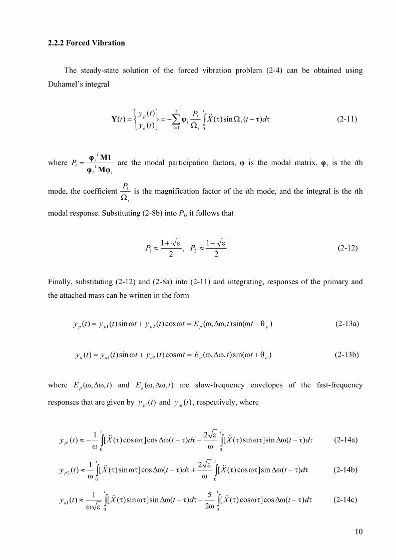
2.2.2 Forced Vibration
The steady-state solution of the forced vibration problem (2-4) can be obtained using
Duhamel’s integral
∑ ∫=
ττ−ΩτΩ
−=
=2
1 0
)(sin)()()(
)(i
t
ii
ii
a
p dtXP
tyty
t &&φY (2-11)
where i
Ti
Ti
iPMφφM1φ
= are the modal participation factors, φ is the modal matrix, φ is the ith
mode, the coefficient
i
i
iPΩ
is the magnification factor of the ith mode, and the integral is the ith
modal response. Substituting (2-8b) into Pi, it follows that
2
11
ε+≈P ,
21
2ε−
≈P (2-12)
Finally, substituting (2-12) and (2-8a) into (2-11) and integrating, responses of the primary and
the attached mass can be written in the form
)sin(),,(cos)(sin)()( 21 ppppp ttEttyttyty θ+ωω∆ω=ω+ω= (2-13a)
)sin(),,(cos)(sin)()( 21 aaaaa ttEttyttyty θ+ωω∆ω=ω+ω= (2-13b)
where and are slow-frequency envelopes of the fast-frequency
responses that are given by and , respectively, where
),,( tE p ω∆ω ),,( tEa ω∆ω
)(ty pi )(tyai
∫∫ ττ−ω∆ωττω
ε+ττ−ω∆ωττ
ω−≈
tt
p dtXdtXty00
1 )(sin]sin)([2)(cos]cos)([1)( &&&& (2-14a)
∫∫ ττ−ω∆ωττω
ε+ττ−ω∆ωττ
ω≈
tt
p dtXdtXty00
2 )(sin]cos)([2)(cos]sin)([1)( &&&& (2-14b)
∫∫ ττ−ω∆ωττω
−ττ−ω∆ωττεω
≈tt
a dtXdtXty00
1 )(cos]cos)([25)(sin]sin)([1)( &&&& (2-14c)
10

∫∫ ττ−ω∆ωττω
+ττ−ω∆ωττεω
≈tt
a dtXdtXty00
2 )(cos]sin)([25)(sin]cos)([1)( &&&& (2-14d)
It can be seen that , , , and all represent oscillations of the system
with slow frequency
)(1 ty p )(2 ty p )(1 tya )(2 tya
ω∆ , with the bracketed terms as external forces. For example, the first term
of (2-14a) represents the slow-frequency “velocity” response subjected to acceleration
, while the second term represents the slow-frequency “displacement” response
subjected to support acceleration . As a result,
ttX ωcos)(&&
tωsintX )(&& ),,( tE p ω∆ω and are both
harmonic functions. Thus, the forced vibration of the tuned system is also characterized by the
presence of beating. What makes a difference in the forced responses is that the beating frequency
is not , but a frequency determined by the forcing frequency and
),,( tEa ω∆ω
ω∆ ω∆ .
When , the forced response of the system can be readily calculated numerically
with Mathematica. For , ,
ttX ω= sin)(&&
A 2−= 50=ω 01.0=ε , and 5=ω∆ , the response is given by Figure
2.3.
0.5 1 1.5 2 2.5t
-0.002
-0.001
0.001
0.002disp . Response of the Primary Mass
0.5 1 1.5 2 2.5t
-0.04
-0.02
0.02
0.04disp . Response of the Secondary Mass
Figure 2.3: Beat phenomenon in forced vibration
2.3 Analysis of Our Proposed, Weakly Coupled MDOF System
To analytically solve for the eigenvalues and eigenvectors of a multiple degree-of-freedom
system is, in most cases, intractable for n , as the order of the polynomial characteristic
frequency equation is twice the number of DOF n. Design of the secondary system involves
choosing its parameters such that tuning to a resonant frequency of the existing primary system is
achieved. This further increases the complexity of the problem.
3>
11

The system we chose to examine has a total (primary plus secondary) of four degrees of
freedom. The primary system is connected to the secondary system through a very weak spring kb
(Figure 2.4). Due to this weak connection, the two subsystems can be regarded as decoupled when
selecting parameters for tuning. This makes it possible to readily find a partial analytical solution
for this system.
2.3.1 Tuning Algorithm
Consider the undamped linear system (spring kn does not exist) in Figure 2.4. Without loss of
generality, assume the masses of the superstructure to be m and the stiffness coefficients to be k.
The masses of the base and the subfoundation are 1.5m. The coupling stiffness coefficient is
, where ε . kkb ε= 1<<
)(g tx&&
m2
mb
GROUND
k1
mc
x1
m1
k2
kc kb
x2
Primary Structure
ee kn
kn
Figure 2.4: Our proposed linear system
Stiffness kc is to be tuned to one mode of the primary structure, which consists of the base
and superstructure. Accounting for the weak stiffness of kb, the lowest system natural frequency
will be nearly zero, corresponding to the almost rigid-body mode of the primary structure. The
second and third natural frequencies will be non-zero, and one of them will be used to tune the
subfoundation. In this study, the first deformational frequency of the primary structure, 2pω , is
chosen to be tuned with the subfoundation. On physical grounds, the resonant frequency is chosen
to be the frequency of the first mode in which the base-structure combination would experience
significant inter-story displacements.
12

Considering the linear system consisting of the base and superstructure, we can readily
compute its natural frequencies from the stiffness and mass matrices of (2-15):
, (2-15)
=
mm
m
p
5.1000000
M
ε+−−−
−=
kkkkk
kk
p
)1(02
0K
where subscript p represents the primary system. Frequencies pω are found by solving
. The determinant is reduced to the polynomial equation (2-16),
where λ .
0|||| 1 =λ−=λ− − IKMID ppppp
2pp ω=
02)()68()()211(3 223 =ε+λε++λε+−λ−mk
mk
ppp (2-16)
This equation can be solved if ε is given a value. Let 033.0=ε , i.e. 301 ; then
mk
p 0093.01 =λ , mk
p 8301.02 =λ , mk
p 8483.23 =λ (2-17)
This ε is small enough for the beating phenomenon to occur. It will be used through this Thesis.
The tuning spring coefficient is determined from 2pc ω=ω , where the resonant frequency of
the isolator degree of freedom is c
bcc m
kk +=ω . Thus,
k kkm pcc 2122.12 =ε−λ= (2-18)
and then tuning process is complete.
2.3.2 Vibration Analysis
Once kc is selected, the natural frequencies and mode shapes of the entire structure can be
determined. The mass and stiffness matrices of the system are
13

M , K (2-19)
=
mm
mm
5.100005.100000000
+εε−ε−ε+−
−−−
=
kkkkk
kkkkk
)2122.1(00)1(0
0200
The dynamical matrix D of the full structure is, for 033.0=ε ,
mk
−−−
−−−
== −
8301.0022.000022.06887.06667.0001210011
1KMD (2-20)
Setting | = 0 gives the eigenvalues |ID λ−
mk00906.01 =λ ,
mk81488.02 =λ ,
mk84547.03 =λ ,
mk84982.24 =λ (2-21)
The circular frequencies, λ=Ω , are
mk0952.01 =Ω ,
mk9027.02 =Ω ,
mk9195.03 =Ω ,
mk6880.14 =Ω (2-22)
and the natural frequencies in Herze. are πΩ 2 , or
mkf 0151.01 = ,
mkf 1437.02 = ,
mkf 1463.03 = ,
mkf 2687.04 = (2-23)
Note that and ( and ) are very close, which will lead the system to beat. Frequencies
and Ω can be rewritten as
2Ω
3
3Ω 2f 3f
2Ω
2202 ω∆−ω=Ω , 2203 ω∆−ω=Ω (2-24)
14

where mk9111.020 =ω ,
mk0084.02 =ω∆ . Note that 20ω is nearly equal to the tuning
frequency mk
mk
pp 9111.08301.022 ≈=λ=ω .
Solving for the modal vectors φ from [ ] 0φID =λ− gives
φ , , , (2-25)
=
2607.09729.09909.01
1
−−
=
1311.17806.0
18511.01
2φ
−=
1733.18216.0
1545.01
3φ
−
−=
0062.05707.08493.11
4φ
whereφ is the modal matrix and φ is the ith modal vector. Figure 2.5 graphically depicts the
mode shapes, which have all been normalized to unity at story 2 for uniformity.
i
Figure 2.5: Mode shapes of the linear 4 DOF system
Again, free vibration is the linear superposition of the four modes. Around the tuned
frequencies 2202 ω∆−ω=Ω , 2203 ω∆−ω=Ω ,
])sin[(])sin[()( 222032122021 θ+ω∆+ω+θ+ω∆−ω= tAtAt φφY (2-26)
Assume , and 121 == AA 021 =θ=θ
15

ttttt 2022320232 cos]sin)[(sin]cos)[()( ωω∆−+ωω∆+= φφφφY
≈ (2-27)
ωω∆−ωω∆+
tttt
20223
20232
cos]sin)[(sin]cos)[(
φφφφ
Equation (2-27) indicates that free vibration of the tu
( ) vibration modulated by slow-frequency (20ω 2ω∆ ) v
The forced response, on the other hand, is the su
factors and modal responses of each mode as
∑ ∫=
τΩ
−=4
1 0
sin)()(i
t
i
ii X
Pt &&φY
where y represents displacement with respect to the gro
, )()()( txtytx g+=
=
(((
)( 1
2
yyyy
t
c
b
Y
and i
Ti
Ti
iPMφφM1φ
= are the modal participation fa
, , and 0255.1 2 =P1 =P 4350.0− 4101.03 =P 4 −=P
factors are km10.7721 ,
km0752.2 ,
km446.0 0.446
From the above analysis, we can see that if the s
frequency content close to the tuned frequency 2pω , it
to the resonance effect, while its peak responses fall o
periodic vibration. In this condition, the first and the
combined effect is small. This can be
that are shown in Figure∫ ττ−Ωτ=t
ii dtXtA0
)(sin)()( &&
primary structure
subfoundation
ned 4DOF system is also a fast-frequency
ibration.
mmation of the products of magnification
ττ−Ω )(i dt (2-28)
und; i. e.,
(2-29)
))))(
tttt
ctors. In this example with 033.0=ε ,
0005.0 , the corresponding magnification
0, and km0003.0 , respectively.
ystem is subjected to ground motions with
will vibrate at the fast tuned frequency due
n the envelope of the slow-frequency ( ω∆ )
fourth modes can be ignored, because their
verified from the modal responses
2.6.
16

1 2 3 4 5 6t
-0.0075-0.005-0.0025
0.00250.0050.0075
A1 1st Modal Amplitude
1 2 3 4 5 6 t
-0.75-0.5-0.25
0.250.50.75
A2 2nd Modal Amplitude
1 2 3 4 5 6t
-0.75-0.5-0.25
0.250.50.75
A3 3rd Modal Amplitude
1 2 3 4 5 6t
-0.01
-0.005
0.005
0.01A4 4th Modal Amplitude
Figure 2.6: Resonant modal responses to harmonic ground excitation
It can be seen that, although the magnification factor of the 1st mode is five times that of the
2nd mode and 24 times that of the 3rd mode, the modal amplitudes of the 2nd and the 3rd modes are
100 times that of the 1st mode. So the response is mainly determined by the 2nd and the 3rd modes,
such that
∫∫ ττ−ΩτΩ
−ττ−ΩτΩ
−=t
g
t
g dtxP
dtxPt0
33
33
02
2
22 )(sin)()(sin)()( &&&& φφY
∫∫ ττ−ω∆−ωτΩ
−ττ−ω∆+ωτΩ
−t
g
t
g dtxP
dtxP
0220
3
33
0220
2
22 )])(sin[()()])(sin[()( &&&& φφ=
ttqPPtq
PP2023
3
32
2
213
3
32
2
2 sin)]()()()[ ωΩ
−Ω
+Ω
−Ω
− φφφφ=
ttqPPtq
PP2043
3
32
2
233
3
32
2
2 cos)]()()()[( ωΩ
+Ω
−+Ω
+Ω
φφφφ+
(2-30)
where
17
q , q (2-31a) ∫ ττ−ω∆τωτ=t
g dtxt0
2201 )(coscos)()( && ∫ ττ−ω∆τωτ=t
g dtxt0
2202 )(sinsin)()( &&
q , q (2-31b) ∫ ττ−ω∆τωτ=t
g dtxt0
2203 ])(cossin)()( && ∫ ττ−ω∆τωτ=t
g dtxt0
2204 )(sincos)()( &&
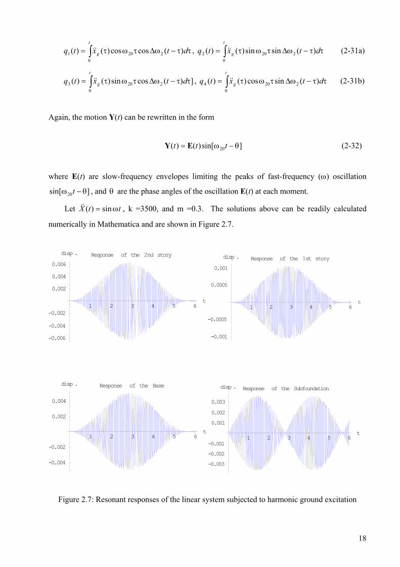
Again, the motion Y(t) can be rewritten in the form
]sin[)()( 20 θ−ω= ttt EY (2-32)
where E(t) are slow-frequency envelopes limiting the peaks of fast-frequency (ω) oscillation
, and θ are the phase angles of the oscillation E(t) at each moment. ]sin[ 20 θ−ω t
Let , k =3500, and m =0.3. The solutions above can be readily calculated
numerically in Mathematica and are shown in Figure 2.7.
ttX ω= sin)(&&
1 2 3 4 5 6t
-0.006-0.004
-0.002
0.0020.0040.006
disp . Response of the 2nd story
1 2 3 4 5 6 t
-0.001
-0.0005
0.0005
0.001disp . Response of the 1st story
1 2 3 4 5 6 t
-0.004
-0.002
0.002
0.004
disp . Response of the Base
1 2 3 4 5 6t
-0.003-0.002-0.001
0.0010.0020.003
disp . Response of the Subfoundation
Figure 2.7: Resonant responses of the linear system subjected to harmonic ground excitation
18

It is apparent from these plots that there is energy transfer between the subfoundation and the
primary system.
For more complicated cases, where resonance does not occur, i. e., , the 1pg ω≠ω st mode
and the 4th mode cannot be ignored. Analysis for these conditions carried out numerically in
Matlab and Simulink. Model building in Simulink will be discussed in Chapter 4, and numerical
results will be given in Chapter 6.
19

Chapter 3: Estimation of the Undamped Nonlinear Normal Modes
3.1 Description of the System
The model of the nonlinear base-isolated structure is depicted in Figure 3.1. It is essentially
identical to the four-degree-of-freedom linear model discussed in the previous chapter, except that
the linear spring k with clearance has been added between ground and the subfoundation m .
The primary structure to be isolated consists of a 2-DOF superstructure plus a base mass. The
base is weakly and linearly coupled to an intermediate or secondary system which itself is
connected to ground through a bilinear hardening spring, which is simply the parallel combination
of two linear springs, one having a clearance nonlinearity. The intermediate system consists of the
subfoundation m
n e c
c and linear spring kc, which acts in conjunction with the clearance spring to
localize the ground input energy away from the primary structure. This is achieved by tuning the
absorber to a mode of the superstructure to be isolated so that internal resonance occurs. The
clearance spring kn acts to excite the appropriate localized nonlinear normal mode, while the
clearance e is a design parameter which determines the onset of nonlinear behavior.
)(g tx&&
m2
mb
GROUND
k1
mc
x1
m1
k2
kc kb
x2
Primary Structure
ee kn
kn
Figure 3.1: Schematic of the proposed system
The desired response of the complete structure to ground motion would resemble a nonlinear
normal mode (NNM) in which motion is almost entirely confined to the intermediate
subsystem—a localized mode in which the base and superstructure participate very little. We will
demonstrate that this nonlinear design is capable of localizing energy away from the primary
structure by examining the modal structure in the region of the internal resonance. To facilitate
20

the analysis to follow, a smooth stiffness to ground, composed of the sum of linear and cubic
terms, is presumed, as analysis employing non-smooth nonlinearity is beyond the scope of this
thesis.
Let x represent displacement with respect to a fixed reference frame and y displacement
with respect to ground, and let subscripts g and c represent ground and subfoundation,
respectively. Then, the equations of motion of the system are
m
(3-1)
−−=−+−+−+=−+−+−+−+=−+−+−+−+
=−+−+
)()()()(0)()()()(0)()()()(
0)()(
1111
212112121111
12212222
gcbcbbcbgcccc
bcbbbcbbbb
bb
xxFxxkxxcxxcxmxxkxxkxxcxxcx
xxkxxkxxcxxcxmxxkxxcxm
&&&&&&
&&&&&&
&&&&&&
&&&&
For free vibration, equations (3-1) can be rewritten as
m
(3-2)
−=−+−+−+=−+−+−+−+=−+−+−+−+
=−+−+
)()()()(0)()()()(0)()()()(
0)()(
1111
212112121111
12212222
cbcbbcbgcccc
bcbbbcbbbb
bb
yFyykyycxycymyykyykyycyycy
yykyykyycyycymyykyycym
&&&&&&
&&&&&&
&&&&&&
&&&&
where the restoring force provided by the cubic nonlinearity is given by
(3-3) 3)( ukukuF nc +=
while the restoring force provided by the clearance nonlinearity is given by
− (3-4)
++
−+=
)(
)()(
eukukuk
eukukuF
nc
c
nc
eueue
eu
−<≤≤
>
We replace this by the smooth nonlinearity in (3-3) for the purpose of this analysis.
The linear spring coefficient kc is used to tune the subfoundation or intermediate subsystem
to one of the modes of the primary structure; kc will be determined through the tuning process, as
has been discussed in Chapter 2. To ensure that the design embodies the requirements of weak
linear coupling between the base and the intermediate subsystem, we set
21
cb k1
1α
=k , cn kk 2α= (3-5)
where α1 and α2 are values greater than one. Through this tuning procedure, all parameters
needed for the design of the intermediate system can be specified.
3.2 Undamped NNMs Using the Complexification-Averaging Method
The objective of this chapter is to find analytical forms of the NNMs of the undamped
system, as their structure will tell us much about the response of the damped, forced system.
Here, we find the steady-state NNMs for the smooth cubic nonlinearity.
We note that both linear and nonlinear systems admit single-frequency exponential solutions.
So, in this context, NNMs can be regarded as solutions that possess exponential temporal
dependence; i.e., solutions that consist of a “fast” oscillation with frequency ω modulated by a
“slow” envelope. The existence of the strongly nonlinear term in the fourth equation of (3-2)
prohibits the use of standard perturbation techniques for analyzing the dynamics. However, as
shown in Manevitch (2001), Vakakis (2001), and Jiang (2002), the dynamics of (3-2) can be
studied analytically by complexification and averaging. This simplifies the associated
computations and leads to results that are physically meaningful. Averaging relies on the
transformation of the equations of motion to an averaged set, which is more easily examined.
To this end we introduce the complex quantities
U , V)()()( tyityt bb ω+= & )()()( 11 tyityt ω+= & ,W )()()( 22 tyityt ω+= & , )()()( tyitytS cc ω+= &
(3-6)
In terms of these variables, the accelerations, velocities, and displacements can be expressed as
ω+
=+
=+
ω−=
ω−
=+
=+
ω−=
ω−
=+
=+
ω−=
ω−
=+
=+
ω−=
itStStytStStytStSitSty
itWtWtytWtWtytWtWitWty
itVtVtytVtVtytVtVitVty
itUtUtytUtUtytUtUitUty
ccc
bb
2)()()(,
2)()()(,
2)()()()(
2)()()(,
2)()()(,
2)()()()(
2)()()(,
2)()()(,
2)()()()(
2)()()(,
2)()()(,
2)()()()(
***
*
2
*
2
*
2
*
1
*
1
*
2
***
2
&&&&
&&&&
&&&&
&&&&
(3-7)
22
where i is the imaginary unit and * denotes the complex conjugate. Substituting (3-7) into (3-2),
the equations of motion are complexified and assume the form
=ω
−−+
+−
++
ω−
+ω
−−+
++
ω−
−+ω
−
=+
+−
−+ω
−−
ω−
+
+−
++
ω−
+ω
−−++
ω−
=+
+−−
+ω
−−
ω−
+
+−
++
ω−
+ω
−−++
ω−
=+
+−−
+ω
−−
ω−
++ω
−
0]2
)([)22
(
]2
)(2
)([22
)()](2
[
0)22
(]2
)(2
)([
)22
(]2
)(2
)([)](2
[
0)22
(]2
)(2
)([
)22
(]2
)(2
)([)](2
[
0)22
(]2
)(2
)([)](2
[
3***
*****
****
**
1
**
1*
**
1
**
1
**
2
**
2*
1
**
2
**
2*
2
SSikUUSSc
UUiSSikSScSSikSSiSm
UUSScUUiSSik
VVUUcVViUUikUUiUm
VVUUcVViUUik
WWVVcWWiVVikVViVm
WWVVcWWiVVikWWiWm
nb
bccc
bb
b
&
&
&
&
(3-8)
Since we seek steady-state vibrations of approximate frequency ω, we express the complex
variables in polar form
(3-9)
ωµ+µ=⇒µ=⇒ϕ=ωλ+λ=⇒λ=⇒ϕ=
ωσ+σ=⇒σ=⇒ϕ=ωϕ+ϕ=⇒ϕ=⇒ϕ=
ωωω−ω
ωωω−ω
ωωω−ω
ωωω−ω
titititi
titititi
titititi
titititi
etiettSettSettSetiettWettWettWetiettVettVettVetiettUettUettU
)()()()()()()()()()()()()()()()()()()()()()()()()()()()(
**
**
**
**
&&
&&
&&
&&
where , , and are complex amplitudes representing slowly varying complex
envelopes of the steady state motion. Substituting (3-9) into (3-8) and retaining only terms
containing the fast frequency ω, we obtain the complex modulation equations that govern the
slow dynamics (i.e., the envelope) of the response.
)(tϕ )(tσ )(tλ )(tµ
=ω
µµ−
ϕ−
µ+
ωϕ
+ωµ
−+µ
+ωµ
−µω
+µ
=ϕ
+µ
−+ωϕ
−ωµ
+ϕ
+σ
−+ωσ
+ωϕ
−+ϕω
+ϕ
=ϕ
−σ
+ωσ
−ωϕ
+σ
+λ
−+ωλ
+ωσ
−+σω
+σ
=σ
−λ
+ωλ
−ωσ
+λω
+λ
08
3)
22()
22(
22)
2(
0)22
()22
()22
()22
)2
(
0)22
()22
)22
()22
()2
(
0)22
()22
()2
(
3
*2
11
11221
222
nbbccc
bbb
ikciikcikim
ciikciikim
ciikciikim
ciikim
&
&
&
&
(3-10)
23

In deriving the above equations we have omitted higher harmonics in the fast oscillation.
There can exist subharmoic or superharmonic steady state responses, but the error resulting from
this approximation is not expected to be large for the fundamental frequency-amplitude plots that
will be discussed here.
For steady-state motions, the amplitudes of the above complex variables must vary much
more slowly than those with fast frequencies. Thus, we set their derivatives equal to zero in (3-
10); i.e., 0)( =tϕ& , 0)( =tσ& , , and 0)( =tλ& 0)( =tµ& , and we obtain the set of equations that
governs the amplitudes and phases of the envelope modulations,
=ω
µµ−ϕ−
ω+µ++
ω−
ω−ω
=µ−ω
+σ−ω
+ϕ++ω
−ω
−ω
=ϕ−ω
+λ−ω
+σ++ω
−ω
−ω
=σ−ω
+λ+ω
−ω
04
3)()(
0)()()(
0)()()(
0)()(
3
*2
1111
112212211
22222
nbbbcbcc
bbbbb
ikcikccikikmi
cikcikccikikmi
cikcikccikikmi
cikcikmi
(3-11)
To analyze (3-11) we express the complex variables in terms of their real and imaginary
components,
, σ , )()()( 21 tixtxt +=ϕ )()()( 21 tiytyt += )()()( 21 tiztzt +=λ , )()()( 21 titt ν+ν=µ (3-12)
Substituting (3-12) into (3-11), and separately setting equal to zero the real and imaginary parts,
we obtain eight real algebraic equations governing the eight new coordinates. These eight
equations are solved numerically in Mathematica.
From (3-5), (3-8) and (3-12), we recover the relationships between the complex amplitudes
and original coordinates; e. g.,
)sin))(cos()(()()()()( 1122 tittzitzettxitxtW ti ωω+ωω+=λ=ω+= ω&
Thus,
)sin(||1)(2 λθ+ωλω
= ttx , )cos(||)(2 λθ+ωλ= ttx& (3-13a)
Similarly,
24

)sin(||1)(1 σθ+ωσω
= ttx , )cos(||)(1 σθ+ωσ= ttx& (3-13b)
)sin(||1)( ϕθ+ωϕω
= ttxb )cos(||)( ϕθ+ωϕ= ttxb& (3-13c)
)sin(||1)( µθ+ωµω
= ttxc , )cos(||)( µθ+ωµ= ttxc& (3-13d)
where amplitudes are given by 22
21| zz +=λ| , and phase angles by
1
21tanzz−
λ =θ , etc.
This completes the theoretical analysis.
3.3 Numerical Results for Undamped NNMs
3.3.1 Physical Parameters for Estimation
We need to choose parameters of the system for numerical solution of equations (3-11). The
values selected are given in Table 3.1. These are consistent with the tuning criteria for the
isolation system outlined above. Damping has been neglected at this stage.
Table 3.1: Physical parameters of the system
Superstructure Base Intermediate System
m1, m2 0.2 kg mb 0.3 kg mc 0.3 kg
k1, k2 3500 N/m kb 116 N/m kc 4242 N/m
kn 2×10⁶kc N/m3
To replace the cubic nonlinearity with a bilinear clearance element, we chose the stiffness
coefficient of the clearance spring k cn k10= and the clearance 0009.0=e m. The resulting
smooth nonlinear restoring force, F , and its bilinear counterpart, are shown in
Figure 3.2.
3ukn)( uku c +=
25

-0.002 -0.001 0.001 0.002u
-75
-50
-25
25
50
75FHuL
Figure 3.2: Nonlinear restoring force
3.3.2 Solutions of the Algebraic Equations
Of the eight algebraic equations, six are linear and two are cubic. Using Guassian
elimination, the eight equations are reduced to two nonlinear equations
0)])((1[ 22
211 =+ω+ zzfz
(3-14) 0)])((1[ 22
212 =+ω+ zzfz
where is a function of . )(ωf ω
It can be seen from (3-14) that, for each ω ,
)(
122
21 ω
−=+f
zz (3-15)
where 22
21 zz + is the slow oscillation amplitude of the 2nd story. Other complex variables and,
hence, amplitudes in (3-12) can all be deduced linearly from z and . Thus, this is the only
amplitude solution for this problem. Equation (3-15) indicates that z and can be purely
imaginary for some values of ω . This is acceptable, as inspection reveals that, at these
frequencies, purely imaginary solutions are equivalent to purely real solutions, and vice versa.
1 2z
1 2z
From (3-15) we see that, though 22
21 zz + is a constant for each ω , and can be
arbitrary. For this problem, it is sufficient, then, to consider only the case z , since the
remaining solutions can be found by rotating this one by
1z
1
2z
0=
)|)(|
1arctan(ω
±f
in the plane. )2z,( 1z
26

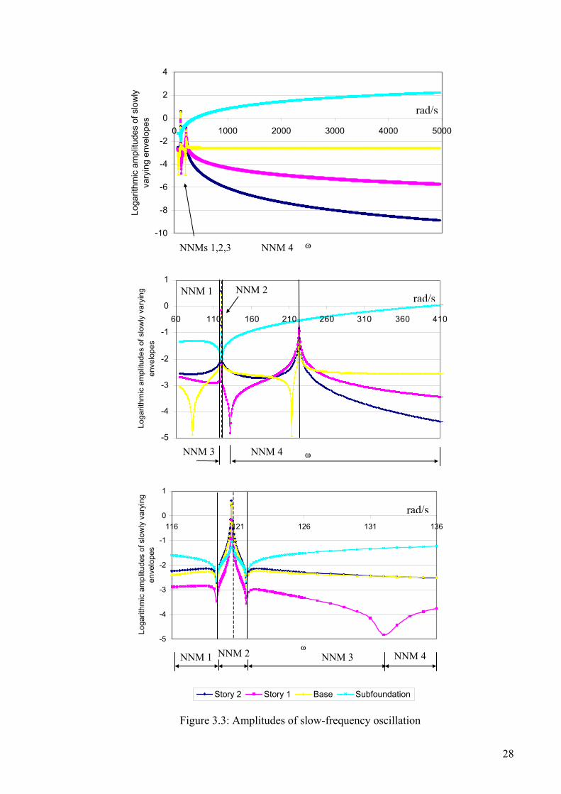
3.3.3 Figures and Discussion
Figure 3.3 depicts the amplitude versus frequency plots for the system with the cubic
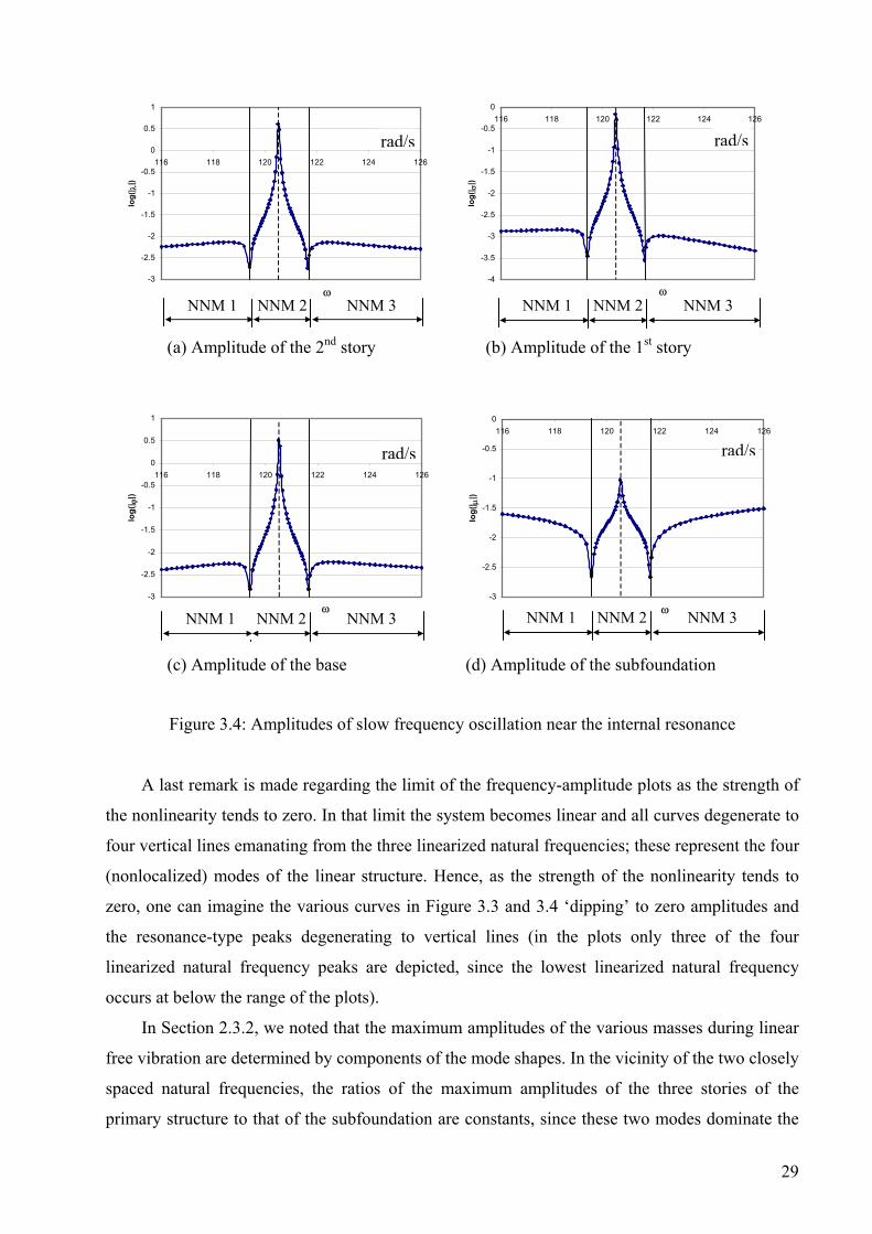
nonlinearity. Figure 3.4 presents the enlargement of the plots in Figure 3.3 near the internal
resonance point. The straight vertical lines represent the linear bending modes ( 0=nk ), at
frequencies rad/s, rad/s, and 415.119=ω 636.121=ω 296.223=ω rad/s. The dotted line is the
1st bending mode of the primary structure (the mode to which the subfoundation is tuned), where
. This coincides with the frequency of the tuning algorithm discussed in Chapter 2.
The mode shapes of the linear system (without the stiffness nonlinearity) are independent of
frequency, and can be found only to within a multiplicative constant at their respective natural
frequencies.
523.120=ω
The curves of Figures 3.3 and 3.4 represent the nonlinear normal modes of the undamped
system with the local nonlinearity, i.e., the free, synchronous periodic solutions of the unforced
system (Vakakis et al., 1996). It can be seen that NNM shapes (i.e., the relative displacements of
the masses of the system) are functions of frequency. In the region near a tuning frequency, one
notes that both stories of the main structure, the base and the subfoundation, undergo resonance-
type behavior (they possess sharp local maxima versus frequency, though, since no external
harmonic excitation exists, one cannot technically characterize this local behavior as ‘resonance’),
with the two stories and the base vibrating at relatively large amplitudes compared to the
subfoundation. It is concluded, therefore, that near the tuning region ‘inverse localization’ of the
free vibration to the main structure and away from the foundation occurs. In fact, the point where
the amplitude of story 1 tends to zero can be used to distinguish between the different branches of
NNMs of the system, which in the plots are labeled from 1 to 4. In this system due to the localized
nature of the nonlinearity there exist four NNMs (equal in number to the modes of the
corresponding linear structure), and they can be considered as analytic continuations for the
nonlinear case of the linear modes of the system with no stiffness nonlinearity; in other words, no
NNM bifurcations were detected in the system examined.
Outside of the tuning region, however, NNM 4 becomes localized at the subfoundation for
increasing frequency. This conclusion is drawn by the increase in the amplitude of the
subfoundation with simultaneous decrease of the amplitudes of the two stories. It is this high-
frequency nonlinear localization of NNM 4 to the subfoundation that gives rise to the motion
confinement phenomena discussed in the next sections.
27
-10
-8
-6
-4
-2
0
2
4
0 1000 2000 3000 4000 5000
ω
Loga
rithm
ic a
mpl
itude
s of
slo
wly
va
ryin
g en
velo
pes
s
3 NNM 4
-5
-4
-3
-2
-1
0
1
60
Loga
rithm
ic a
mpl
itude
s of
slo
wly
var
ying
en
velo
pes
-5
-4
-3
-2
-1
0
1
116
Loga
rithm
ic a
mpl
itude
s of
slo
wly
var
ying
enve
lope
s
NNMs 1,2,
110 160 210 260 310 360 410
NNM 2
NNM 4
s NNM 1
F
NNM 3
ω121 126 131 136
ω
s
NNM 4
NNM 1S
igure 3
NNM 2
tory 2 Story 1 Ba
.3: Amplitudes of slow
NNM 3
se Subfoundation
-frequency oscillation
rad/
rad/
rad/
28
-3
-2.5
-2
-1.5
-1
-0.5
0
0.5
1
116 118 120 122 124 126
log(
| λ|)
-4
-3.5
-3
-2.5
-2
-1.5
-1
-0.5
0116 118 120 122 124 126
log(
| σ|)
s
ω ωNNM 1 NNM 2 NNM 3 NNM 1 NNM 2 NNM
(a) Amplitude of the 2nd story (b) Amplitude of the 1st story
-3
-2.5
-2
-1.5
-1
-0.5
0
0.5
1
116 118 120 122 124 126
ω
log(
| ϕ|)
-3
-2.5
-2
-1.5
-1
-0.5
0116 118 120 122 124
ω
log(
| µ|)
s
NNMNNM 2 NNM 1NNM 3NNM 2 NNM 1
(c) Amplitude of the base (d) Amplitude of the subfoundation
Figure 3.4: Amplitudes of slow frequency oscillation near the internal resonan
A last remark is made regarding the limit of the frequency-amplitude plots as the
the nonlinearity tends to zero. In that limit the system becomes linear and all curves de
four vertical lines emanating from the three linearized natural frequencies; these repres
(nonlocalized) modes of the linear structure. Hence, as the strength of the nonlinear
zero, one can imagine the various curves in Figure 3.3 and 3.4 ‘dipping’ to zero amp
the resonance-type peaks degenerating to vertical lines (in the plots only three
linearized natural frequency peaks are depicted, since the lowest linearized natura
occurs at below the range of the plots).
In Section 2.3.2, we noted that the maximum amplitudes of the various masses d
free vibration are determined by components of the mode shapes. In the vicinity of the
spaced natural frequencies, the ratios of the maximum amplitudes of the three sto
primary structure to that of the subfoundation are constants, since these two modes d
rad/s
rad/3
126
s
c
e
i
o
l
u
t
o
rad/
rad/3
e
strength of
generate to
nt the four
ty tends to
litudes and
f the four
frequency
ring linear
wo closely
ries of the
minate the
29

free response and the linear mode shapes are invariant. Thus, the amplitude ratios are straight
lines in configuration space. In Figure 3.5, we plot both linear and nonlinear modal amplitudes of
the three stories of the primary structure versus that of the subfoundation for comparison
purposes.
0
0.003
0.006
0.009
0.012
0.015
0 0.004 0.008 0.012 0.016 0.02 0.024 0.028 0.032
| µ |
| σ |
0
0.01
0.02
0.03
0.04
0.05
0 0.004 0.008 0.012 0.016 0.02 0.024 0.028 0.032
| µ || λ
|
(a) 1st story vs. the subfoundation (b) 2nd story vs. the subfoundation
0
0.01
0.02
0.03
0.04
0.05
0 0.004 0.008 0.012 0.016 0.02 0.024 0.028 0.032
| µ |
| φ |
(c) The base vs. the subfoundation
Figure 3.5: Modal amplitudes of the primary structure vs. the subfoundation
The straight lines in Figure 3.5 represent the linear normal modes. Curves above the straight
lines are nonlinear normal modes near the resonant frequency, while curves below the straight
lines are outside of the resonant frequency range. Figure 3.5 shows that the nonlinear normal
modes in this system are curves instead of straight lines. In the terminology of Rosenberg (1960)
these are nonsimilar NNMs.
30
Chapter 4: Model Building for System Analysis in Simulink
4.1 Introduction
From the analysis in Chapter 2, we see that, even for an idealized linear 2DOF system
(Figure 2.1) subjected to simple harmonic excitation, the analytical solution can be somewhat
complicated. In view of the fact that we wish to explore relatively large-scale MDOF nonlinear
structures, finding solutions analytically is not practical. Thus, we resort to available analysis
tools, such as Matlab and Simulink, to perform numerical calculations. In this chapter we will
discuss how we built simulation models corresponding to the system of Figure 3.1 in Simulink.
Simulink is a sophisticated graphical user interface (GUI) that complements Matlab for with
modeling, simulating, and analyzing dynamical systems. It supports linear and nonlinear systems,
modeling in continuous or discrete time or a hybrid of the two. Its modeling environment uses
familiar block diagrams, so systems illustrated in texts can be easily implemented in Simulink
(Dabney and Harman, 1998).
4.2 Elements of a Model
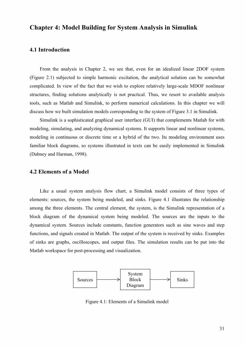
Like a usual system analysis flow chart, a Simulink model consists of three types of
elements: sources, the system being modeled, and sinks. Figure 4.1 illustrates the relationship
among the three elements. The central element, the system, is the Simulink representation of a
block diagram of the dynamical system being modeled. The sources are the inputs to the
dynamical system. Sources include constants, function generators such as sine waves and step
functions, and signals created in Matlab. The output of the system is received by sinks. Examples
of sinks are graphs, oscilloscopes, and output files. The simulation results can be put into the
Matlab workspace for post-processing and visualization.
System Block
Diagram Sinks Sources
Figure 4.1: Elements of a Simulink model
31

Simulink includes a comprehensive library of sinks, sources, linear and nonlinear
components, and connectors. One can also customize and create blocks. After a model is defined,
one can simulate it, using a choice of solvers, and then execute it either from the Simulink menus
or by entering commands in the Matlab command window. In our Simulink code, the isolation
system is represented by a scalar model while the two-story building is described by a vector
(state-space) model. These will be discussed in the next section.
4.3 Scalar System: the Nonlinear Isolation System
Consider the nonlinear oscillator of the proposed isolation system, depicted in Figure 4.2.
mb ekn
yb(t)+xg(t) yc(t)+xg(t) xg(t)
kbkc
mc
Figure 4.2: The scalar nonlinear system
Let y represent displacement with respect to the ground and z, displacement with respect to the
base mass mb. Then, with subscripts g and c representing ground and subfoundation, respectively,
gcg xyzxyx ++=+= (4-1)
Referring to equations (3-1), the equations of motion of the subfoundation mc and base mb may be
written as
gc
cg
c
ccbcbbcbcccc
cc x
mk
xmc
yFxxkxxcxkxcm
x ++−−−−−−−= &&&&&& )]()()([1 (4-2)
0)]()()()([1111 =−+−+−+−−= cbcbbbcbb
bb xxkxxkxxcxxc
mx &&&&&& (4-3)
The restoring force in (4-2) provided by the nonlinear spring-gap element is given by
32

− (4-4)
++
−+=
)(
)()(
eukukuk
eukukuF
nc
c
nc
eueue
eu
−<≤≤
>
The equations have been rewritten so that the system inputs are ground velocity and displacement
instead of commonly used ground acceleration, as will be explained in detail in Chapter 5. Figure
4.3 shows the Simulink model of the subfoundation.
System Block Diagram Sinks Sources
Figure 4.3: The Simulink model of the subfoundation
Oval blocks represent inputs and outputs, rectangular blocks (with + and - signs),
summation, and triangular blocks, gains. Scalar input signals to the subfoundation mc include
ground velocity and displacement, linear spring restoring forces and damping forces produced by
their relative motion to base and to ground, and the nonlinear restoring force. The outputs of the
system are scalar signals of accelerations, velocities and displacements and are displayed by
oscilloscopes. The central diagram is where the dynamic differential equation is solved. The
velocity and the displacement are obtained by numerically integrating the acceleration. We set the
initial conditions to zero, because the system is at rest before the ground moves. The nonlinear
restoring force is modeled by a dead-zone block and a function block.
The Simulink model of the base can be built in the same way as that of the subfoundation,
except that it is linear and its input forces result from its motion relative to the subfoundation and
the first story mass.
33

4.4 Vector (State-Space) Linear System: the Superstructure
For linear MDOF systems, it is often convenient to use vector signals, as they provide a more
compact and easier-to-understand model. The state-space approach is particularly useful for
modeling linear systems, because we can take advantage of matrix notation to describe very
complex systems in a compact form. Additionally, we can compute the system response using
matrix arithmetic. Before discussing model building using vectors, let’s discuss the concept of
state variables and describe the state-space block in Simulink first.
The general form of the state-space model of a dynamical system is
x ),,( tuxf=& (4-5)
where is the state vector, u the input vector, and t time. Equation (4-5) is called the system
state equation. We also define the system output equation to be
x
y ),,( tuxg= (4-6)
In linear spring-mass-damper systems, the system state equation and the output equation can
be written as linear combinations of the system states and inputs as
x BuAx +=& (4-7) y DuCx += (4-8) where matrix A is called the system matrix, B the input matrix, C the output matrix, and D the
direct transmittance matrix. Equations (4-7) and (4-8) comprise the state-space block in Simulink.
To use state-space block to model the linear superstructure, we first rewrite the equations of
motion of the two-story superstructure with the base velocity and the base displacement as input
0)()( 12212222 =−+−+ xxkxxcx &&&&m (4-9)
m bb xcxkxxkxkxxcxcx &&&&&& 11212112121111 )()( +=−++−++ (4-10)
The matrix equation representing the dynamics of the two-story superstructure is
m )()()()( tttt uDkxxcx 1−=++ &&& (4-11)
34

where
m , c , , (4-12)
=
2
1
00
mm
−
−+=
22
221
ccccc
−
−+=
22
221
kkkkk
k
x , , (4-13)
=)()(
)(2
1
txtx
t
=
0011
1
ckD
=)()(
)(txtx
tb
b
&u
The state-space equation of motion for the superstructure of this system is
(4-14) )()()(
)()( 1 t
tt
tt
u0
Dxx
m00k
xx
0mmc
=
−
+
&&&
&
Note that the boldface zeros in (4-14) represent 22× null matrices.
Define the state vector ξ , and so ξ . It follows that the system state
equation is
=)()(
)(tt
txx&
=)()(
)(tt
txx&&
&&
ξ (4-15) BuAξ +=&
where
A , B (4-16) 211AA −= 1
11BA −=
A , A , (4-17)
=
0mmc
1
−
=m00k
2
=0
DB 1
1
If the output variables are the system state variables, then ξy = , and the output equation is
ξ DuCξ += (4-18)
where
C , D (4-19) I=
=
00000000
This is shown in Figure 4.4, block “StateSpace1”.
35
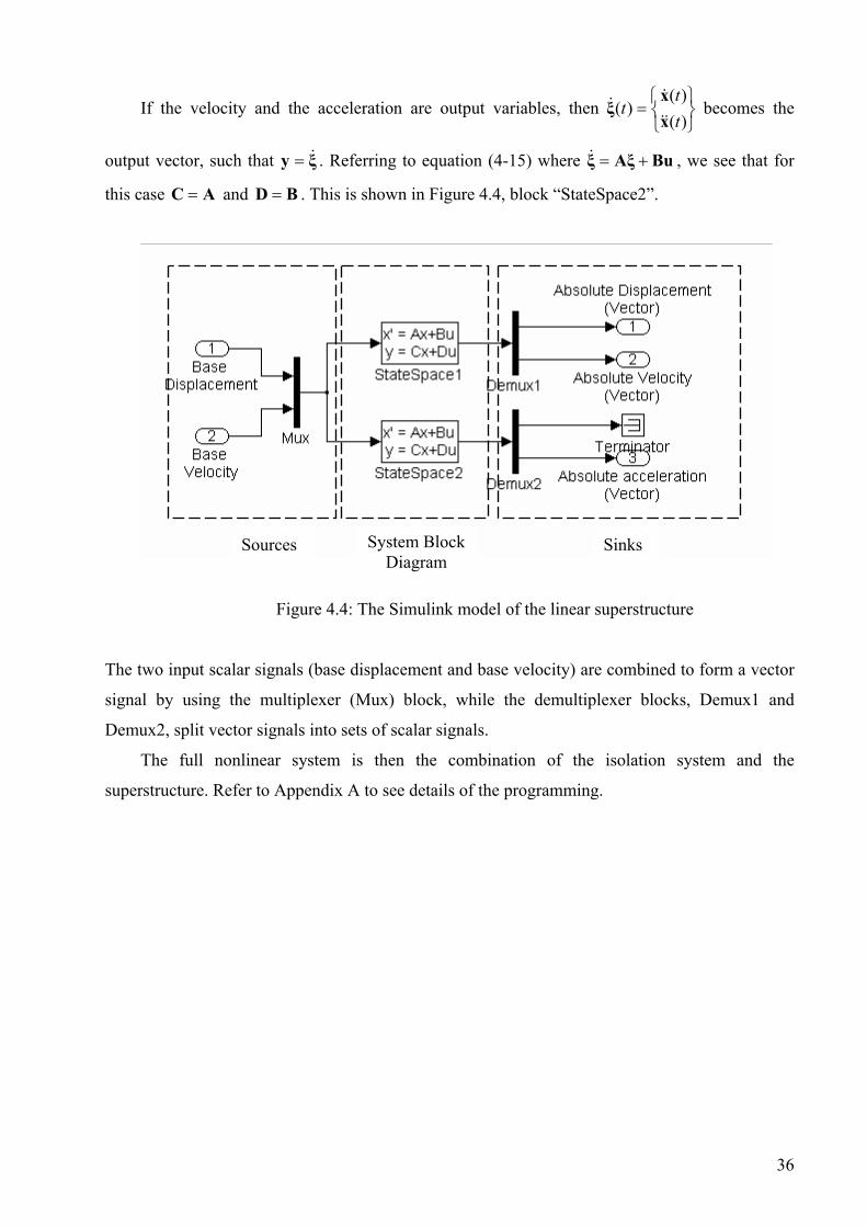
If the velocity and the acceleration are output variables, then ξ becomes the
output vector, such that y . Referring to equation (4-15) where ξ , we see that for
this case C and . This is shown in Figure 4.4, block “StateSpace2”.
=)()(
)(tt
txx&&
&&
BuAξ +=ξ&=
B=
&
A= D
System BlockDiagram
Sources Sinks
Figure 4.4: The Simulink model of the linear superstructure
The two input scalar signals (base displacement and base velocity) are combined to form a vector
signal by using the multiplexer (Mux) block, while the demultiplexer blocks, Demux1 and
Demux2, split vector signals into sets of scalar signals.
The full nonlinear system is then the combination of the isolation system and the
superstructure. Refer to Appendix A to see details of the programming.
36

Chapter 5: Ground Motions Considered In This Study
5.1 Introduction
The dynamic response of a structure depends on its mechanical characteristics and the nature
of the excitation. A protective system that efficiently controls the response of the structure when
subjected to certain classes of inputs may not be efficient when subjected to other classes. For
example, long-period pulses contained in near field earthquake records decrease the performance
of passive viscous dampers (Malhotra, 1999). Hence, the usual method of using randomly chosen
ground motions or assuming simple filtered white noise excitation models may not lead to an
effective protective system.
Previous studies have demonstrated that near field earthquakes contain coherent long-period
pulses with some overriding high-frequency fluctuations (Anderson et al., 1986, Iwan and Chen,
1994). These long-period pulses are sometimes distinguishable even in the acceleration time
history. Peak ground acceleration (PGA) is the most commonly used measure of earthquake
potential. However, studies indicated that what makes near field ground motions particularly
destructive to flexible structures is not their PGA but their long-duration pulse, which represents
the incremental velocity that the above-ground mass has to reach (Anderson and Bertero, 1986,
Hall et al., 1995, Iwan, 1997). The peak ground displacement (PGD) is not a reliable measure
either, since the displacement history is the second integral of the acceleration history, and the
long-period components may be filtered out (He, 2003). The peak ground velocity (PGV) seems
to be a better representative measure of earthquake destructiveness as it represents the cumulative
effect of the seismic energy radiating from the fault for near field ground motions (Somervill and
Graves, 1993).
These long-period pulses present a challenge to the concept of base isolation for earthquake
protection. Although recent design codes have incorporated near field effects in the design
spectrum, the design procedure is the same as that for ordinary ground motions. Furthermore, in
addition to earthquakes, structures will experience a number of transient excitations throughout
their lives, some of which may also exhibit these characteristics. Hence, it is imperative to study
the kinematic characteristics of near field effects from available records for shock-protective
systems.
Makris (1997) and Makris and Chang (1998) proposed closed-form velocity-pulse models
for near field ground motions. Based on these studies, He (2003) proposed an analytical model for
velocity pulses and systematically studied the properties of the proposed pulse model. It was
37

verified from response spectra and curve-fitting analyses that this model could capture the major
characteristics of near field earthquakes. Thus, in this study we use velocity pulses and velocity
time histories other than the usual accelerograms as the inputs to account for near-field effects.
We will introduce these models briefly, and then explain which of them will be employed in this
study.
5.2 Makris and Chang’s Model
Makris and Chang (1998) grouped velocity pulses present in near field ground motions into
three types of pulses: the type A pulse, the type B pulse, and type Cn pulses, represented by a
unique set of tri-geometric functions. Type A is a forward-only pulse; type B is a full sine wave
pulse that approximates a forward-and-back motion; and type Cn pulses approximate an n-cycle
ground displacement. The formulations of these velocity pulse types are given by
Type A: )cos1(2
)( tv
tx pp
p ω−=& , pTt ≤≤0 (5-1)
Type B: tvtx ppp ω= sin)(& , pTt ≤≤0 (5-2)
Type Cn: ϕ−ϕ+ω= sin)sin()( pppp vtvtx& , pTnt )21(
πϕ
−+≤≤0 (5-3)
where subscript p denotes “pulse”.
There is a permanent ground displacement at the end of the Type A pulse, while the ground
displacement of type B fully recovers to its initial value. In order to have a zero ground
displacement at the end of a type Cn pulse, the condition
(5-4) 0)(0
=∫ dttxT
g&
must be satisfied. Here, T is the duration of a type Cn pulse
ppp TnTnT )21(2)21( πϕ−+=ωϕ−+= (5-5)
with pulse frequency pp Tπ=ω 2 . Substitution of (5-3) and evaluation of the integral (5-4) gives
38
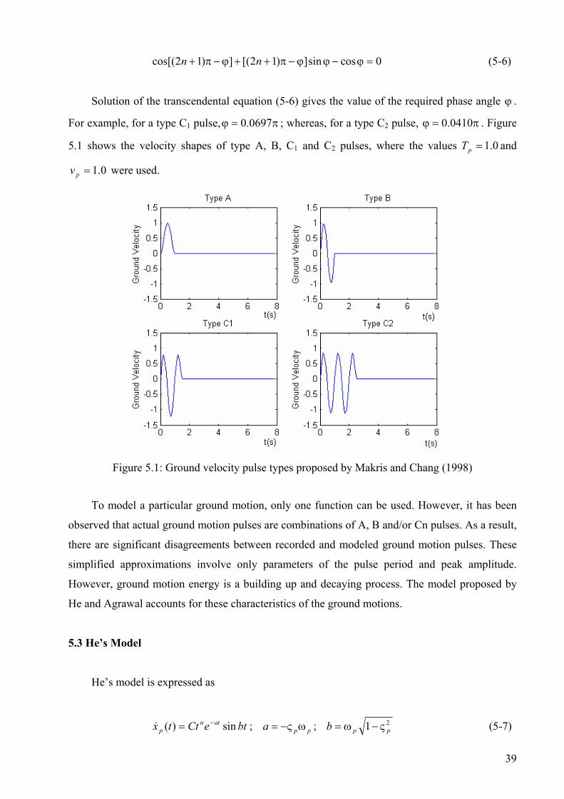
cos[( 0cossin])12[(])12 =ϕ−ϕϕ−π++ϕ−π+ nn (5-6)
Solution of the transcendental equation (5-6) gives the value of the required phase angle ϕ .
For example, for a type C1 pulse, π=ϕ 0697.0 ; whereas, for a type C2 pulse, π= 0410.0ϕ . Figure
5.1 shows the velocity shapes of type A, B, C1 and C2 pulses, where the values 0.1=pT and
were used. 0.1=pv
Figure 5.1: Ground velocity pulse types proposed by Makris and Chang (1998)
To model a particular ground motion, only one function can be used. However, it has been
observed that actual ground motion pulses are combinations of A, B and/or Cn pulses. As a result,
there are significant disagreements between recorded and modeled ground motion pulses. These
simplified approximations involve only parameters of the pulse period and peak amplitude.
However, ground motion energy is a building up and decaying process. The model proposed by
He and Agrawal accounts for these characteristics of the ground motions.
5.3 He’s Model
He’s model is expressed as
; bteCttx atnp sin)( −=& ppa ως−= ; 21 ppb ς−ω= (5-7)
39

Equation (5-7) presumes that the velocity pulse is an enveloped sinusoidal function. The
parameters a and n determine the shape of the pulse envelope, pς is the decay factor, pω is the
frequency, and C is the amplitude constant of the pulse. Figure 5.2 shows the versatility of the
proposed ground velocity pulses generated by different values of parameters n, a and b. It is seen
that the model is capable of generating various types of pulses reminiscent of those observed in
near field earthquake ground motions.
Figure 5.2: Ground velocity pulse models proposed by He (2003)
The ground acceleration is obtained by differentiating equation (5-7) and is given by
]cossin)[()( btbbtatneCttx atn
p +−= −&& (5-8)
While the ground displacement can be obtained by integrating equation (5-7), its explicit form is
quite complicated despite n being an integer.
For the special case of n , the velocity pulse (5-7) is a decaying sine-wave, and the
corresponding ground displacement is
0=
22
)cossin()(ba
bbtbbtaeCtxat
p +++−
=−
(5-9)
40
The velocity pulse in equation (5-7) can be defined in terms of the vector of parameters
as ],,,[ banC=Θ
),()( Θtxtx pp && = (5-10)
To obtain parameters for a particular ground motion, the start time of the pulse, t0, should
also be included in the vector of parameters, i.e., ],,,,[ 0tbanC=Θ . In his thesis, He (2003) also
gave a method to find the parameter vector Θ that best fits a recorded ground velocity . This
is achieved by minimizing the sum of squares of the difference between x and at
discrete time instants t
)(txg&
,( ip tx&)( ig t& )Θ
i,
S , i = 1, 2, 3,…, N (5-11) ∑=
−=N
iipig txtx
1
2)],()([)( ΘΘ &&
where the ti are the discrete times at which the time history is recorded.. )( ig tx&
The minimization of S was done by Newton’s method in this analysis. Using the
minimization procedure, He (2003) obtained optimal parameter vectors for 36 recorded ground
motions from around the world.
)(Θ
5.4 Ground Motions Employed in This Thesis
5.4.1 Full Sine Wave Ground Velocity
The first input we will examine is a ground velocity shock pulse, which imparts a large
amount of energy to the structure in a short time. From Makris and Chang, we adopt the type B
model, i.e., the forward-and-back sine-wave, because it is simple, and the final displacement will
be zero at the end of the ground motion. This type of velocity pulse, and its corresponding
acceleration and displacement, can be expressed as
tT
vtxp
ppπ
=2sin)(& , pTt ≤≤0 (5-12)
tT
vT
txp
pp
pππ
=2cos2)(&& , pTt ≤≤0 (5-13)
41
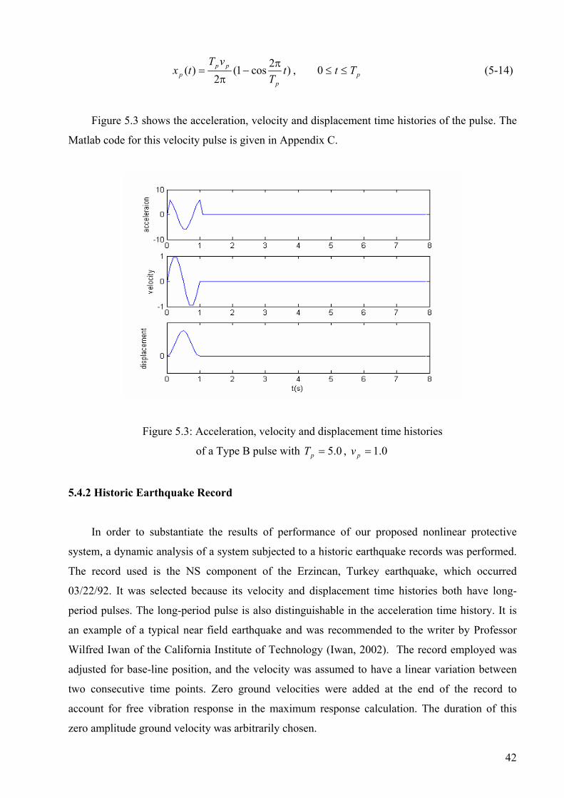
)2cos1(2
)( tT
vTtx
p
ppp
π−
π= , pTt ≤≤0 (5-14)
Figure 5.3 shows the acceleration, velocity and displacement time histories of the pulse. The
Matlab code for this velocity pulse is given in Appendix C.
Figure 5.3: Acceleration, velocity and displacement time histories
of a Type B pulse with 0.5=pT , 0.1=pv
5.4.2 Historic Earthquake Record
In order to substantiate the results of performance of our proposed nonlinear protective
system, a dynamic analysis of a system subjected to a historic earthquake records was performed.
The record used is the NS component of the Erzincan, Turkey earthquake, which occurred
03/22/92. It was selected because its velocity and displacement time histories both have long-
period pulses. The long-period pulse is also distinguishable in the acceleration time history. It is
an example of a typical near field earthquake and was recommended to the writer by Professor
Wilfred Iwan of the California Institute of Technology (Iwan, 2002). The record employed was
adjusted for base-line position, and the velocity was assumed to have a linear variation between
two consecutive time points. Zero ground velocities were added at the end of the record to
account for free vibration response in the maximum response calculation. The duration of this
zero amplitude ground velocity was arbitrarily chosen.
42

5.4.3 Approximation by He’s Method
We chose to use a function to simulate ground motions containing near field effects in our
analyses. As He (2003) has already provided optimal model parameters for 36 historic
earthquakes around the world, we employed his results for the Erzincan earthquake record in (5-7)
C cm/s, , 57.70−= 00.5=n 80.1=a , 75.2=b , 6.00 =t s (5-15)
Figure 5.4: Erzincan earthquake time histories and their approximations
The recorded and approximate earthquake ground motions for the first 15 seconds are plotted
in Figure 5.4, where it is apparent that the simulated closed-form velocity time history agrees well
with that of the actual earthquake record. While the displacement time histories are also
comparable, the corresponding acceleration time histories differ, verifying the conjecture that the
approximate velocity can only represent the dominant low frequency component, resulting in
underestimation of peak ground acceleration (He and Agrawal, 2002).
To examine how well the approximated pulse model captures the characteristics of the actual
earthquake, numerical simulations were conducted to compare the dynamic responses of a SDOF
oscillator subjected to the recorded ground motions and those of the He pulse model. Consider a
SDOF oscillator subjected to a ground acceleration . Its equation of motion is )(txg&&
(5-16) )()()(2)( 2 txtytyty g&&&&& =ω+ςω+
43
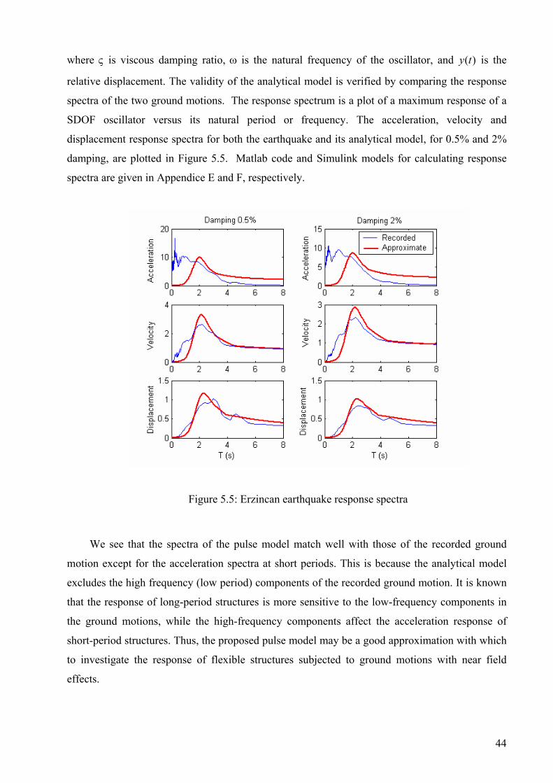
where is viscous damping ratio, ς ω is the natural frequency of the oscillator, and y is the
relative displacement. The validity of the analytical model is verified by comparing the response
spectra of the two ground motions. The response spectrum is a plot of a maximum response of a
SDOF oscillator versus its natural period or frequency. The acceleration, velocity and
displacement response spectra for both the earthquake and its analytical model, for 0.5% and 2%
damping, are plotted in Figure 5.5. Matlab code and Simulink models for calculating response
spectra are given in Appendice E and F, respectively.
)(t
Figure 5.5: Erzincan earthquake response spectra
We see that the spectra of the pulse model match well with those of the recorded ground
motion except for the acceleration spectra at short periods. This is because the analytical model
excludes the high frequency (low period) components of the recorded ground motion. It is known
that the response of long-period structures is more sensitive to the low-frequency components in
the ground motions, while the high-frequency components affect the acceleration response of
short-period structures. Thus, the proposed pulse model may be a good approximation with which
to investigate the response of flexible structures subjected to ground motions with near field
effects.
44
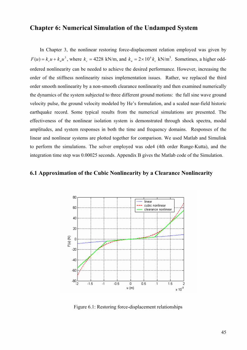
Chapter 6: Numerical Simulation of the Undamped System
In Chapter 3, the nonlinear restoring force-displacement relation employed was given by
, where kN/m, and kN/m3)( ukukuF nc += 4228=ck cn kk 6102×= 3. Sometimes, a higher odd-
ordered nonlinearity can be needed to achieve the desired performance. However, increasing the
order of the stiffness nonlinearity raises implementation issues. Rather, we replaced the third
order smooth nonlinearity by a non-smooth clearance nonlinearity and then examined numerically
the dynamics of the system subjected to three different ground motions: the full sine wave ground
velocity pulse, the ground velocity modeled by He’s formulation, and a scaled near-field historic
earthquake record. Some typical results from the numerical simulations are presented. The
effectiveness of the nonlinear isolation system is demonstrated through shock spectra, modal
amplitudes, and system responses in both the time and frequency domains. Responses of the
linear and nonlinear systems are plotted together for comparison. We used Matlab and Simulink
to perform the simulations. The solver employed was ode4 (4th order Runge-Kutta), and the
integration time step was 0.00025 seconds. Appendix B gives the Matlab code of the Simulation.
6.1 Approximation of the Cubic Nonlinearity by a Clearance Nonlinearity
Figure 6.1: Restoring force-displacement relationships
45

To replace the cubic nonlinearity with a bilinear clearance element, we chose the stiffness
coefficient of the clearance spring k cn k10= and the clearance 0009.0=e m. For relative
displacement of the subfoundation with respect to ground less than or equal to 0.002 m, the force-
displacement relationships for the linear, cubic nonlinear, and bilinear clearance springs are
plotted in Figure 6.1. It can be seen that the bilinear clearance nonlinearity and the cubic
nonlinearity are very close for the selected parameters. For the same parameters used in Chapter
3 and the newly specified kn, the natural frequencies and periods of the system and its component
parts are shown in Table 6.1.
Table 6.1: Natural frequencies and periods of the system
Superstructure Superstructure +Base
Linear system (kn = 0)
Linear system (e = 0)
2.259 2.203 2.229 18.9 19.21 13.01 19.21 19.42 35.54
f ( Hz )
34.07 35.54 35.54 62.77 0.4427 0.4539 0.4489
0.0527 0.0521 0.0769 0.0521 0.0515 0.0304
T ( s )
0.0294 0.0281 0.0281 0.0159
1188..99999 1199..22111199..4422 3355..5544
00..00552277 00..0055221100..00551155 00..00330044
Here, we see that the addition of the base and weak spring results in a near rigid-body mode
at 2.259 Hz in the conventionally isolated structure. This becomes 2.203 Hz in the combined
structure incorporating the subfoundation. The first superstructure natural frequency of 19.21 Hz
in the conventionally isolated structure is significantly higher than the lowest fixed-base natural
frequency of 13.01 Hz, demonstrating the effect of a standard isolation system on the
deformational natural frequencies of the structure. The introduction of the subfoundation and
tuning results in two very close natural frequencies at 18.99 Hz and 19.42 Hz, which provide the
internal resonance in the linear system required for localization.
6.2 Response to Full Sine-Wave Ground Velocity Pulses
As described in Chapter 5, we first use the Makris and Chang Type B pulse model (i.e., a full
sine-wave pulse) to examine the dynamics of the proposed system.
tvtx ppp ω= sin)(& , pTt ≤≤0 (5-2)
46

The amplitude of the velocity shock pulse used is pg gv ω= 1 ; thus the corresponding amplitude
of acceleration is 1g.
6.2.1 Shock Spectra
In order to compare the performance of a specified system under the action of different
transient inputs, we plotted the maximum value of a various response quantities versus the
transient pulse duration T . This plot is known as the shock spectrum in the general vibration
literature and the response spectrum in the earthquake engineering literature. The shock spectra
for the nonlinearly isolated building and for the same system with k (i.e., a fully linear
isolation system incorporating the subfoundation) are shown in Figure 6.2. The clearance e used
here is always one-fourth of the peak value of from the linear case.
g
0=n
)(tyc
Figure 6.2: Shock spectra of various responses to a full sine ground velocity pulse
It can be seen that the motion of the subfoundation is limited because of the clearance
nonlinearity and that the nonlinear isolation system suppresses the response in the range of the
two closely coupled linear normal modes (when the pulse width is small) and subharmonic
resonances (when the pulse width is large). In the following, we employ a high frequency (small
period) input pulse to investigate the difference in performance between the linear and nonlinear
47
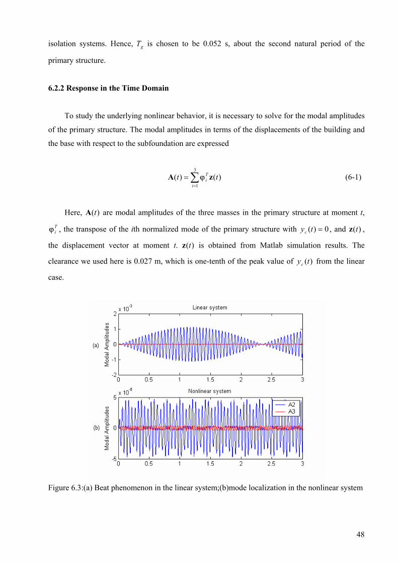
isolation systems. Hence, T is chosen to be 0.052 s, about the second natural period of the
primary structure.
g
6.2.2 Response in the Time Domain
To study the underlying nonlinear behavior, it is necessary to solve for the modal amplitudes
of the primary structure. The modal amplitudes in terms of the displacements of the building and
the base with respect to the subfoundation are expressed
A (6-1) ∑=
=3
1)()(
i
Ti tt zϕ
Here, are modal amplitudes of the three masses in the primary structure at moment t,
, the transpose of the ith normalized mode of the primary structure with , and z ,
the displacement vector at moment t. is obtained from Matlab simulation results. The
clearance we used here is 0.027 m, which is one-tenth of the peak value of from the linear
case.
)(tATiϕ 0)( =tyc
)(tyc
)(t
)(tz
Figure 6.3:(a) Beat phenomenon in the linear system;(b)mode localization in the nonlinear system
48

Note that, in the linear case, the system was designed such that the natural frequency of the
uncoupled subfoundation is equal to one of the natural frequencies of the primary structure. As a
result, when weak coupling between the two subsystems is introduced, we expect a beat
phenomenon to occur, whereby energy from one subsystem transfers to the other and back again.
This is shown in Figure 6.3(a), in which the second and third modal coordinates of the primary
structure are plotted together.
Now, consider the corresponding nonlinear system under the action of the same ground
velocity pulse. Previous studies tell us that the nonlinear system with internal resonance and weak
coupling between the subsystems has a localized NNM. As a result, energy is mainly confined to
the secondary subsystem, and a relatively small portion of this energy ‘leaks’ to the superstructure
(Vakakis et al, 1999). This is presented in Figure 6.3(b). Note the localization effect, the very
small 2nd modal amplitudes that occur in the motion of the primary structure. A2 has been reduced
by 2 orders of magnitude in the nonlinear case. Where did the energy go? It will be shown later
that energy mainly goes to the higher nonlinear modes of the structure. Modal amplitudes of
higher modes are usually very small, as A3 in Figure 6.3.
Figure 6.4: Time history responses to the full sine-wave velocity pulse
Linear Nonlinear
We can examine the dynamics in the displacement and acceleration response time histories.
These are shown in Figure 6.4. Here, the peak responses of the primary structure and linear
subfoundation are out of phase, indicating energy transfer between the two subsystems.
Examination of the nonlinear responses shows that both the inter-story drifts (left column) and the
49
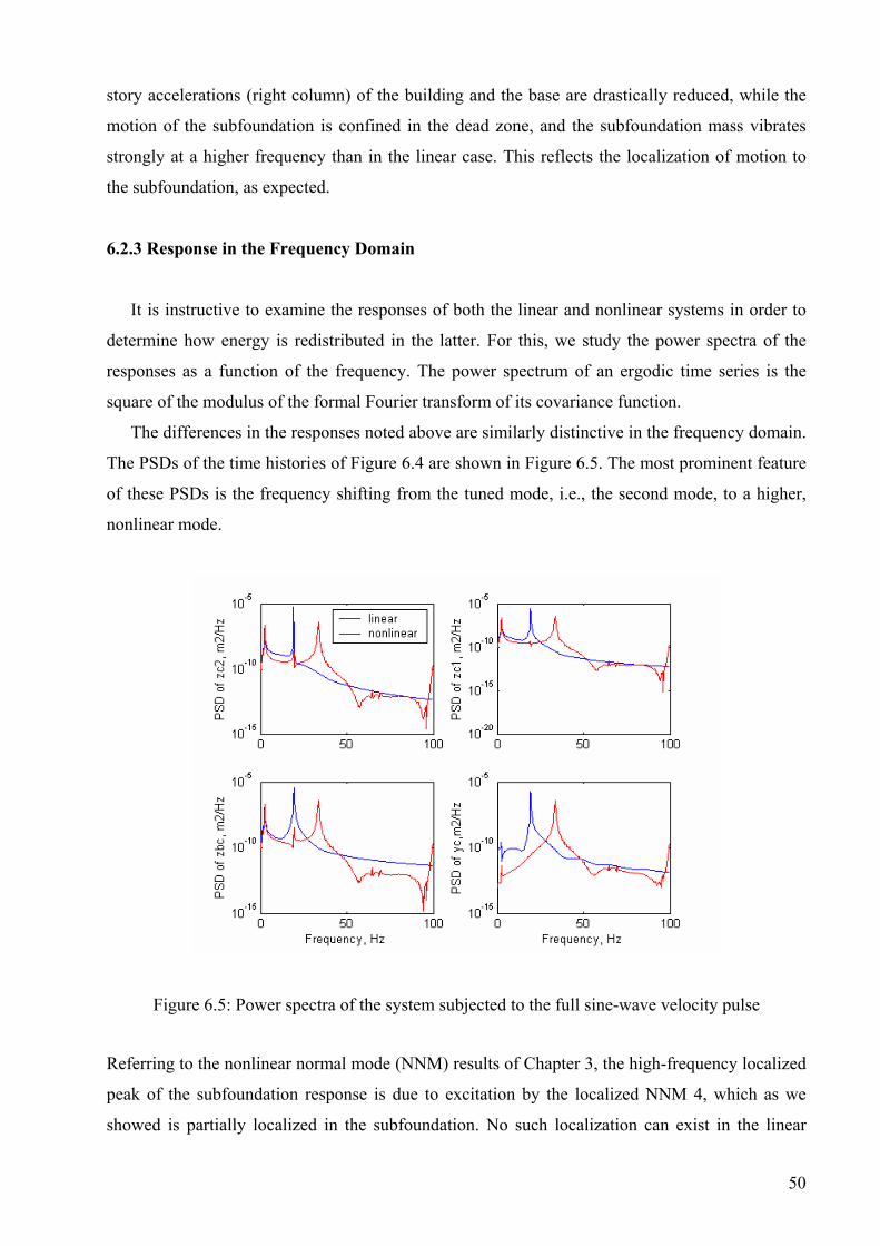
story accelerations (right column) of the building and the base are drastically reduced, while the
motion of the subfoundation is confined in the dead zone, and the subfoundation mass vibrates
strongly at a higher frequency than in the linear case. This reflects the localization of motion to
the subfoundation, as expected.
6.2.3 Response in the Frequency Domain
It is instructive to examine the responses of both the linear and nonlinear systems in order to
determine how energy is redistributed in the latter. For this, we study the power spectra of the
responses as a function of the frequency. The power spectrum of an ergodic time series is the
square of the modulus of the formal Fourier transform of its covariance function.
The differences in the responses noted above are similarly distinctive in the frequency domain.
The PSDs of the time histories of Figure 6.4 are shown in Figure 6.5. The most prominent feature
of these PSDs is the frequency shifting from the tuned mode, i.e., the second mode, to a higher,
nonlinear mode.
Figure 6.5: Power spectra of the system subjected to the full sine-wave velocity pulse
Referring to the nonlinear normal mode (NNM) results of Chapter 3, the high-frequency localized
peak of the subfoundation response is due to excitation by the localized NNM 4, which as we
showed is partially localized in the subfoundation. No such localization can exist in the linear
50
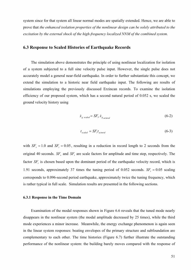
system since for that system all linear normal modes are spatially extended. Hence, we are able to
prove that the enhanced isolation properties of the nonlinear design can be solely attributed to the
excitation by the external shock of the high-frequency localized NNM of the combined system.
6.3 Response to Scaled Histories of Earthquake Records
The simulation above demonstrates the principle of using nonlinear localization for isolation
of a system subjected to a full sine velocity pulse input. However, the single pulse does not
accurately model a general near-field earthquake. In order to further substantiate this concept, we
extend the simulation to a historic near field earthquake input. The following are results of
simulations employing the previously discussed Erzincan records. To examine the isolation
efficiency of our proposed system, which has a second natural period of 0.052 s, we scaled the
ground velocity history using
acturalgVscaledg xSFx && = (6-2)
t acturaltscaled tSF= (6-3)
with and , resulting in a reduction in record length to 2 seconds from the
original 40 seconds. SF and are scale factors for amplitude and time step, respectively. The
factor is chosen based upon the dominant period of the earthquake velocity record, which is
1.91 seconds, approximately 37 times the tuning period of 0.052 seconds. SF scaling
corresponds to 0.096-second period earthquake, approximately twice the tuning frequency, which
is rather typical in full scale. Simulation results are presented in the following sections.
0.1=vSF
tSF
05.0=tSF
v tSF
05.0=t
6.3.1 Response in the Time Domain
Examination of the modal responses shown in Figure 6.6 reveals that the tuned mode nearly
disappears in the nonlinear system (the modal amplitude decreased by 25 times), while the third
mode experiences a minor increase. Meanwhile, the energy exchange phenomenon is again seen
in the linear system responses: beating envelopes of the primary structure and subfoundation are
complementary to each other. The time histories (Figure 6.7) further illustrate the outstanding
performance of the nonlinear system: the building barely moves compared with the response of
51
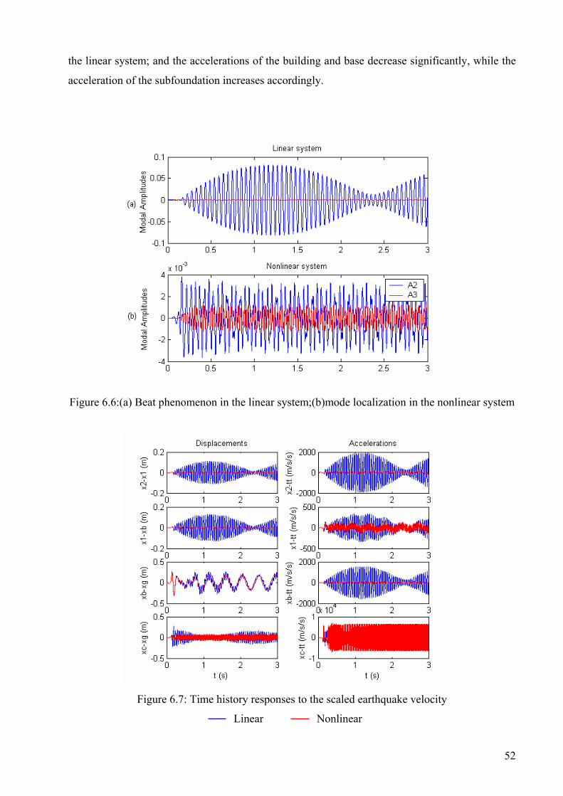
the linear system; and the accelerations of the building and base decrease significantly, while the
acceleration of the subfoundation increases accordingly.
Figure 6.6:(a) Beat phenomenon in the linear system;(b)mode localization in the nonlinear system
Figure 6.7: Time history responses to the scaled earthquake velocity
Linear Nonlinear
52

6.3.2 Response in the Frequency Domain
Figure 6.8: Power spectra of the system subjected to the scaled Erzincan earthquake
The time domain results are confirmed in the frequency domain. From Figure 6.8, we see
that the second mode is completely suppressed, with energy moved to a higher mode at nearly 50
Hz.
6.4 Response to the Analytical (He) Model of Ground Velocity
A systematic investigation of seismic isolation systems applied to reasonably complex
structures subjected to ground motions cannot be accomplished with a limited number of historic
records. It is, therefore, necessary to develop analytical representations of ground motion for use
in parameter studies or Monte Carlo simulation. Here we examine the performance of our
proposed nonlinear isolation system when the structure is subjected to an analytical representation
of the ground velocity determined from the Erzincan earthquake, as described earlier. It was
shown that the analytical formulation (He, 2003) can capture the major characteristics of the
earthquake record, except for high frequency components, which results in underestimation of
acceleration response at high frequencies. As shown previously, the Erzincan earthquake velocity
record is optimally represented by
53
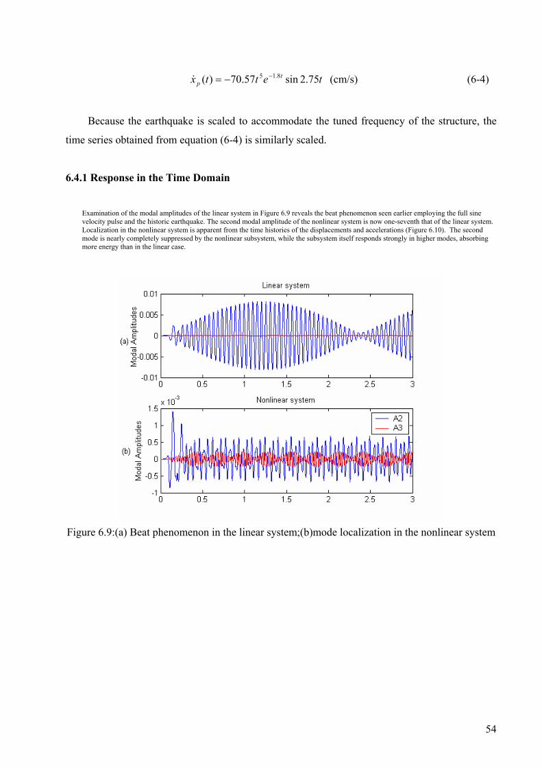
(cm/s) (6-4) tettx tp 75.2sin57.70)( 8.15 −−=&
Because the earthquake is scaled to accommodate the tuned frequency of the structure, the
time series obtained from equation (6-4) is similarly scaled.
6.4.1 Response in the Time Domain
Examination of the modal amplitudes of the linear system in Figure 6.9 reveals the beat phenomenon seen earlier employing the full sine velocity pulse and the historic earthquake. The second modal amplitude of the nonlinear system is now one-seventh that of the linear system. Localization in the nonlinear system is apparent from the time histories of the displacements and accelerations (Figure 6.10). The second mode is nearly completely suppressed by the nonlinear subsystem, while the subsystem itself responds strongly in higher modes, absorbing more energy than in the linear case.
Figure 6.9:(a) Beat phenomenon in the linear system;(b)mode localization in the nonlinear system
54

Figure 6.10: Time history responses to the analytical model of earthquake velocity
Linear Nonlinear
6.4.2 Response in the Frequency Domain
Results in the frequency domain, shown in Figure 6.11, are similar to those obtained
previously for the Erzincan earthquake.
Figure 6.11: Power spectral densities of the system subjected to the full sine-wave velocity pulse
55

Interestingly, the isolation system appears to perform better when subjected to the historic
earthquake record than for its decaying harmonic representation. This is likely attributable to the
fact that the actual earthquake, with its greater energy content, more readily drives the system into
the NNM and resulting localized response. However, the analytical model proves to be useful for
certain kinds of analyses.
56

Chapter 7: Numerical Simulation for the Damped System
7.1 Construction of the Viscous Damping Matrix
7.1.1 Classical Damping Matrix for the Superstructure
Damping in a structure is generally a function of its configuration, materials, construction,
working stresses, environment, boundary conditions, and so forth. The pragmatic analyst usually
presumes that the structure is classically damped, thus avoiding many complicating issues and
facilitating analysis by linear methods. The viscous damping matrix that results is diagonalizable
by the same transformation that uncouples the undamped linear equations of motion.
The norm in the analysis of civil engineering structures, particularly tall buildings, is to
specify the modal damping ratios for a number of modes. A procedure to determine the viscous
damping matrix from modal damping ratios can readily be derived from
ϕ (7-1) Cc =ϕT
where C is the diagonal damping matrix with the nth diagonal element equal to the generalized
modal damping
)2( nnnn M ως=C (7-2)
Here, ς is the nth modal damping ratio, M is the nth modal mass, and ω is the nth circular
natural frequency. Equation (7-1) can also be written as
n n n
c (7-3) 11)( −−= ϕϕ CT
If the nth modal damping ratio ς is not specified, the resulting c assumes a zero damping ratio in
the nth mode.
n
There is a problem associated with the use of the damping matrix given by equation (7-3).
We need story damping for the construction of the damping matrix of the combined (primary plus
isolation) system, as well as for the convenience of numerical simulation. In equations of motion
such as (3-1), the damping matrix is banded, reflecting the close-coupling of the structure; that is,
57
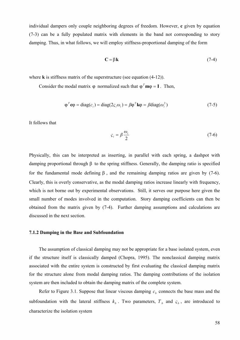
individual dampers only couple neighboring degrees of freedom. However, c given by equation
(7-3) can be a fully populated matrix with elements in the band not corresponding to story
damping. Thus, in what follows, we will employ stiffness-proportional damping of the form
C kβ= (7-4)
where k is stiffness matrix of the superstructure (see equation (4-12)).
Consider the modal matrix normalized such that . Then, ϕ Im =ϕϕT
ϕ (7-5) )diag()diag(2)diag( 2i
Tiii
T ωββωςc ==== ϕϕϕ kc
It follows that
2
ii
ωβ=ς (7-6)
Physically, this can be interpreted as inserting, in parallel with each spring, a dashpot with
damping proportional through β to the spring stiffness. Generally, the damping ratio is specified
for the fundamental mode defining β , and the remaining damping ratios are given by (7-6).
Clearly, this is overly conservative, as the modal damping ratios increase linearly with frequency,
which is not borne out by experimental observations. Still, it serves our purpose here given the
small number of modes involved in the computation. Story damping coefficients can then be
obtained from the matrix given by (7-4). Further damping assumptions and calculations are
discussed in the next section.
7.1.2 Damping in the Base and Subfoundation
The assumption of classical damping may not be appropriate for a base isolated system, even
if the structure itself is classically damped (Chopra, 1995). The nonclassical damping matrix
associated with the entire system is constructed by first evaluating the classical damping matrix
for the structure alone from modal damping ratios. The damping contributions of the isolation
system are then included to obtain the damping matrix of the complete system.
Refer to Figure 3.1. Suppose that linear viscous damping c connects the base mass and the
subfoundation with the lateral stiffness k . Two parameters, T and , are introduced to
characterize the isolation system
b
b b bς
58

b
b ωπ2
=T (7-7)
bbbb mmmc ςω++= )(2 21 (7-8)
where b
bb mmm
k++
=21
ω .
We can interpret T as the natural vibration period and ς as the damping ratio of the base-
structure with the assembly assumed to be a rigid body. With the physical parameters of the
system given in Table 3.1, it follows that
b b
4443.0=b
.01
T s. Compared with the period computed in
Table 7.1, where the nearly rigid-body period is 4427=nT s, we see that the fundamental period
of the base-structure is changed only slightly by the flexibility of the structure.
Damping for the subfoundation can also be specified alone. Assuming its damping ratio is
, the damping coefficient is computed by cς
cccc mc ςω= 2 , where c
bcc m
kkω
+= (7-9)
Table 7.1: Damping coefficients and modal damping ratios
%2=ςb , %1=ςc %5=ςb , ς %1=c
Damping Superstructure Superstructure + Base
Linear system where kn = 0
Superstructure + Base
Linear system where kn = 0
1.86 4.65 1.96 1.51 4.88 2.05 2 3.17 2.21 3.57 3.90
ς (%)
5.24 5.48 5.49 5.53 5.53 c1 1.1723 c2 1.1723 cb 0.3960 0.9899
c (Ns/m)
cc 0.724 0.724
Assuming damping of the fundamental mode of the superstructure to be 2% of critical, the
remaining damping coefficients are calculated and shown in Table 7.1. If damping ratios of the
base and foundation are, respectively, %5=bς and %1=cς , it follows that c Ns/m
and c Ns/m. After all of the damping coefficients are determined, modal damping ratios
9899.0=b
724.0=c
59

for the assembled structure and its component parts can be estimated. These are also presented in
Table 7.1.
Observe that the damping in the first mode of the superstructure-base assembly is, 1.96%
and 4.88%, corresponding to the isolation-rigid body system damping of 2% and 5%,
respectively. Damping in the structure has little influence on the base modal damping, because the
structure behaves almost as a rigid body in this mode. By contrast, high damping of the isolation
system has increased the damping in the first mode of the superstructure from 2% to 3.17% and
3.57%, respectively, for the two values of base isolation system damping. This is a consequence
of nonclassical damping in the assembled system. The coupling terms are nonzero, and so the
modal equations are coupled. As we neglect the coupling terms when calculating the modal
damping ratios, modal analysis provides approximate results.
We see that the modal damping ratios for the fixed-base superstructure increase linearly with
natural frequency because the damping is stiffness proportional. However, as we are concerned
primarily with the tuned modes in the 4DOF isolated system, where the 1st and 2nd modal
damping ratios are approximately 2%, the values chosen are appropriate.
7.2 Response to the Analytical (He) Model of Ground Velocity
The actual earthquake record contains not only low-frequency pulses, but also higher-
frequency components. As shown in Chapter 5, the analytical model by He (2003) captures the
major characteristics of ground motions with near-field effects. Therefore, this model will be
employed to investigate the dynamics of the damped system. The effects of damping in both the
superstructure and subfoundation on the system performance will be investigated. Damping at the
base will also be included in the parametric analysis.
7.2.1 Damping in the Superstructure Only ( 2%ς s = )
Comparing the damped modal responses of Figure 7.1 with the undamped responses of
Figure 6.9, we observe that a small level of damping in the superstructure decreases the amplitude
of the linear 2nd mode response by 2.5 times while the envelopes of the building and
subfoundation remain complementary to each other; in the nonlinear system, the degree of
localization remains nearly the same as in the undamped system. This is expected, as the
necessary conditions for nonlinear localization to occur are internal resonance and suitable
nonlinearity in the isolation system, which are unaffected by damping in the superstructure. This
60

is confirmed by the time history responses in Figure 7.2, where damping in the superstructure
changes the linear superstructure response, while nonlinear responses and responses of the base
and the subfoundation are almost identical to those of the undamped case, with only minor
diminished amplitudes because of energy dissipation.
Figure 7.1: Modal responses of the linear and the nonlinear system (ς ) %2=s
Figure 7.2: Damped time history responses ( %2=sς )
Linear Nonlinear
61

Figure 7.3 Power spectra ( %2=sς )
7.2.2 Damping in the Subfoundation Only ( 2%ς c = )
Figure 7.4 Modal responses of the linear and the nonlinear system ( ) %2ς =c
62

Figure 7.5 Damped time history responses ( ς %2=c )
Linear Nonlinear
Interestingly, 2% damping parallel to the tuning spring is allocated equally to the tuned
modes: the 2nd and 3rd modal damping ratios are both 1%, while the 1st and 4th are nearly zero.
Notice that the ground motion is also scaled to the tuning period, so it is expected that this
damping helps dissipate ground energy and structural energy in the tuned modes. As a result, the
response of the tuned modes decreases and that of the 1st mode increases. The performance of the
nonlinear system compared with that of the linear system is not as impressive, because nonlinear
localization only contributes partly to suppression of the tuned modes, the remainder occurring
through dissipation in common with the linear system.
From Figure 7.4, we see that the maximum amplitude of the 2nd nonlinear modal response
(the tuned mode) is comparable to that of the undamped case, while the maximum amplitude of
the 2nd linear modal response is approximately 40% of that of the undamped case. From the time
history responses (Figure 7.5), it is apparent that both linear and nonlinear systems perform
adequately.
7.3 Parametric Analyses
The clearance e and the clearance spring stiffness kn are design parameters that determine the
strength of the nonlinearity. The smaller gap e and larger kn, the stronger the nonlinearity. In this
63

section, we will discuss how sensitive the performance of the system is to these parameters. It is
desirable to find optimal values of the full parameter set to ensure the best possible design.
However, many factors must be included in the analysis for the nonlinear system to make the
study tractable. Thus, only some qualitative results with examples will be used to illustrate the
necessary steps in this analysis. In additional to the two parameters mentioned previously,
damping at the base level is also included to show the sensitivity of the system to it.
7.3.1 Clearance Size and Clearance Spring Stiffness
In this system, strong nonlinearity helps to drive the input energy into high frequency modes
of the structure, while weak nonlinearity results in a smaller frequency shift. We desire strong
mode localization; thus it seems desirable to shift as much input energy to high frequencies as
possible. In other words, stronger nonlinearity seems desirable. However, this is not the case. By
contrast, excessively large kn decreases the effect of localization and amplifies accelerations; and
making e too small actually results in an untuned linear system which is very sensitive to high-
frequency ground motions. These effects are illustrated in Figures 7.6 through 7.11.
Figure 7.6: Modal responses with a smaller clearance
Figures 6.9 to 6.11 in Chapter 6 showed the undamped responses to the modeled ground
velocity with 008.010/|)_max(| == linyce m. To examine the system sensitivity to e, we give
the modal responses and response power spectra for identical systems incorporating, first, a
64

smaller value of clearance 004.020/|)_max(| == linyc
021.04/|)_max(|
e m, shown in Figures 7.6 and 7.7, and a
larger value of clearance, == linyce m, in Figures 7.8 and 7.9.
Figure 7.7: Power spectra for system with smaller clearance
Comparing Figures 7.6 and 7.7 with Figures 6.9 and 6.11, we see that a smaller clearance
results in better localization; it eliminates the beating in the 3rd mode as well, and shifts the energy
from 35 Hz to 42 Hz.
On the other hand, a large clearance decreases the localization effect for this specific kn.
Though the amplitude of the 2nd mode decreases, the beat phenomenon is still apparent, and the
amplitude of the 3rd mode is large. In Figure 7.8 and 7.9, we see that energy shifts to a frequency
only modestly higher than the resonant frequency. In fact, for cn kk 10= , the best clearance is zero
--- an untuned linear system. It is apparent that the good performance of such a system is not a
result of the tuning-localization algorithm; it just happens that the system is not sensitive to this
particular ground motion.
65
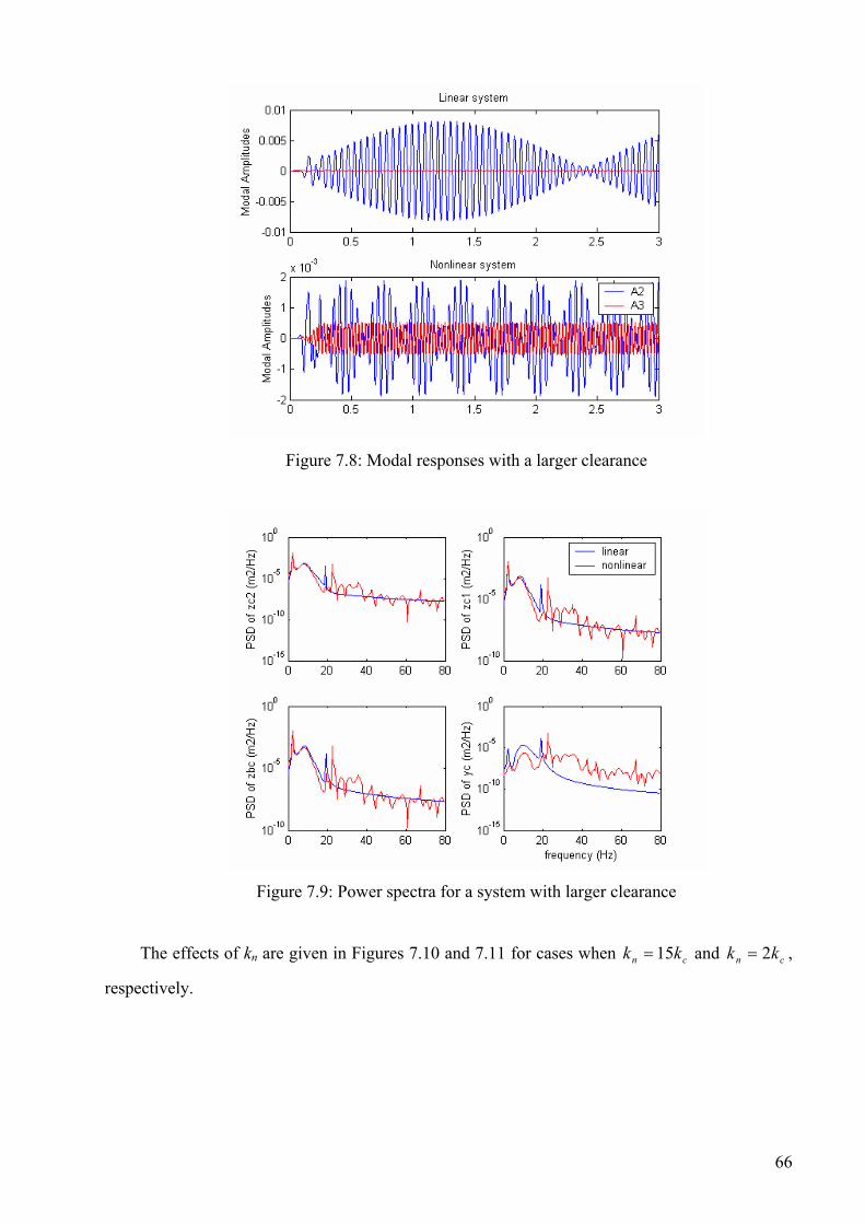
Figure 7.8: Modal responses with a larger clearance
Figure 7.9: Power spectra for a system with larger clearance
The effects of kn are given in Figures 7.10 and 7.11 for cases when k and cn k15= cn kk 2= ,
respectively.
66

Figure 7.10: Modal responses with a larger kn
Figure 7.11: Modal responses with a smaller kn
Here, it can be seen that neither smaller nor larger kn results in improved performance. We
conclude, then that the system performance is not sensitive to kn in this range. However, if
and approaching zero, the system will become the linear tuned system, and the nonlinear
localization effect disappears. For the specified clearance
cn kk 2<
008.010/|)_max(| == linyce m, the
range is reasonably good for nonlinear localization, likely because the resulting
impact forces don’t undergo drastic change.
cn kk 10<<ck2
67

7.3.2 Damping at the Base Only
Figure 7.12: Modal responses of the linear and the nonlinear system ( ) %2ς =b
Figure 7.13: Damped time history responses ( %2ς =b )
Linear Nonlinear
Figure 7.12 shows the linear and nonlinear modal responses with ς . It is apparent
here that damping at the base interrupts the energy interchange between the two subsystems,
%2=b
68

leading to an irregular pattern of beating in the linear case. However, the modal amplitudes do not
experience much of a decrease. In the nonlinear system, localization occurs only in the early
phase when ground motion is large. Time history responses (Figure 7.13) also exhibit this abrupt
change in behavior. In the first phase, the beating phenomenon can be observed in the linear
system, and displacements and accelerations both decrease significantly in the nonlinear system.
In the second phase, the beating is absent in the linear case, and in the nonlinear system
displacement and acceleration responses grow larger, with less energy transfer to the
subfoundation.
It may seem counterintuitive that responses can grow with time in a damped system, while
the external excitation decays to nearly zero. We will examine where the energy causing this
comes from by analyzing the “control” force in the isolation system. By control force, we mean
the impact force, or force generated by impacts in the clearance spring kn. The force in the
clearance spring is expressed by
(7-10)
+
−=
)(0
)()(
euk
eukuF
n
n
c
eueue
eu
−<≤≤−
>
For the undamped response to the modeled ground velocity mentioned in Chapter 6, the control
force and the absolute value of its envelope are shown in Figure 7.14. Matlab code for the force
envelope is given in Appendix D.
Figure 7.14: Control force and force envelope in the undamped system
69
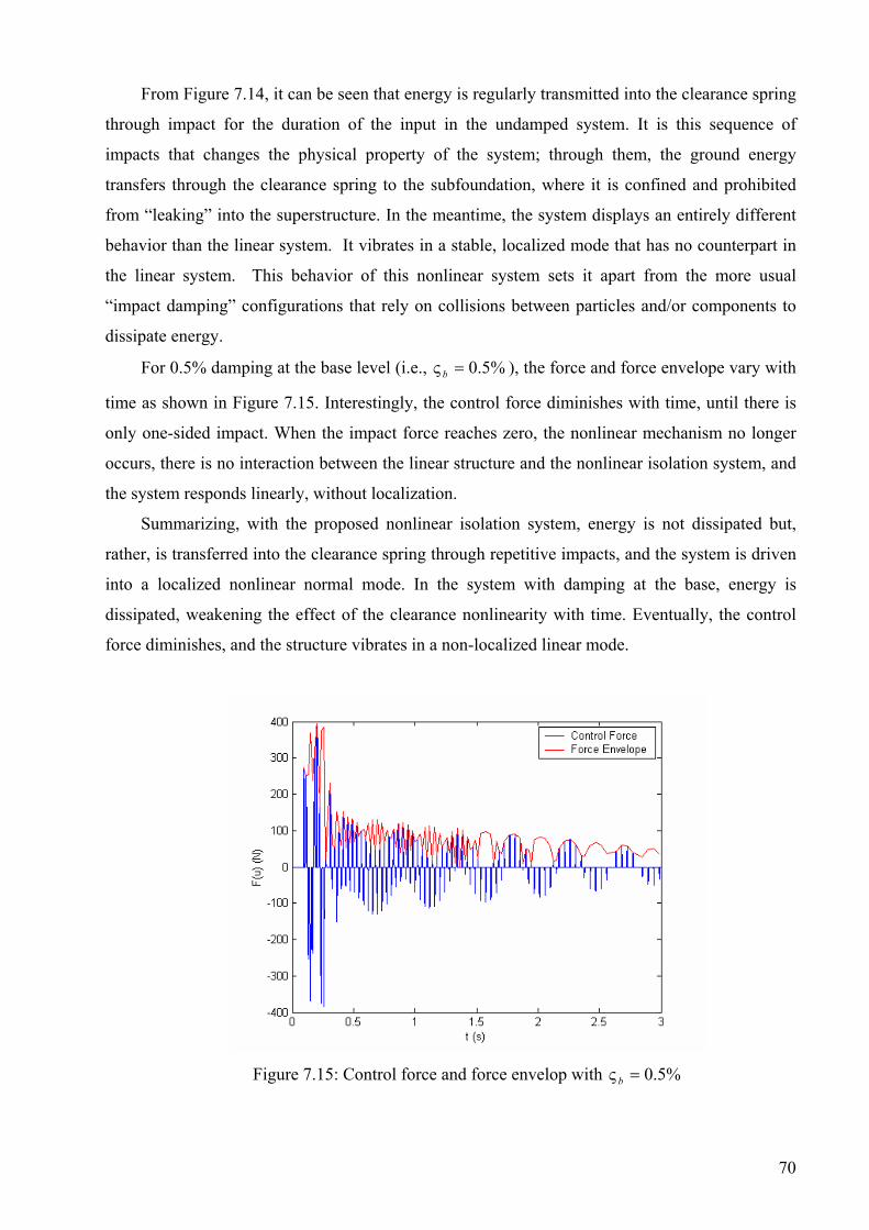
From Figure 7.14, it can be seen that energy is regularly transmitted into the clearance spring
through impact for the duration of the input in the undamped system. It is this sequence of
impacts that changes the physical property of the system; through them, the ground energy
transfers through the clearance spring to the subfoundation, where it is confined and prohibited
from “leaking” into the superstructure. In the meantime, the system displays an entirely different
behavior than the linear system. It vibrates in a stable, localized mode that has no counterpart in
the linear system. This behavior of this nonlinear system sets it apart from the more usual
“impact damping” configurations that rely on collisions between particles and/or components to
dissipate energy.
For 0.5% damping at the base level (i.e., %5.0=ςb ), the force and force envelope vary with
time as shown in Figure 7.15. Interestingly, the control force diminishes with time, until there is
only one-sided impact. When the impact force reaches zero, the nonlinear mechanism no longer
occurs, there is no interaction between the linear structure and the nonlinear isolation system, and
the system responds linearly, without localization.
Summarizing, with the proposed nonlinear isolation system, energy is not dissipated but,
rather, is transferred into the clearance spring through repetitive impacts, and the system is driven
into a localized nonlinear normal mode. In the system with damping at the base, energy is
dissipated, weakening the effect of the clearance nonlinearity with time. Eventually, the control
force diminishes, and the structure vibrates in a non-localized linear mode.
Figure 7.15: Control force and force envelop with %5.0=ςb
70

This effect of damping at the base is further examined in Figure 7.16, where force envelopes
for different damping levels are plotted.
Figure 7.16: Control force envelop for varying damping levels
Here, it is clear that even a small change in damping at the base can greatly decrease the
control force. However, if the clearance e is decreased, thus maintaining the control force, the
performance is likely to improve. To examine this hypothesis, we halved the clearance used in the
example of Figures 12 and 13, for 004.020/|)_max(| == linyce m.
Figure 7.17: Control force envelop for %2=ςb and a smaller clearance
71

In Figure 7.17, we compare the control forces corresponding to base damping of 2% for the
two clearance levels. Clearly, the impacts persist for the smaller clearance, thus prolonging the
nonlinear behavior and resulting localization.
Finally, examination of the response of the system in Figure 7-18 with 2% base damping and
smaller clearance reveals that the second mode response has been further suppressed by a modest
amount, at the expense of the third mode response, which increases slightly. Note the growth in
second mode response once the control force, shown in the previous plot, goes to zero.
Figure 7.18: Modal responses for %2=ςb and a smaller clearance
72

Chapter 8: Comparison of the Nonlinear Isolation System with
Conventional Base Isolation
In the last two chapters, we examined the responses of the nonlinear system subjected to the
scaled ground velocity history that models the Erzincan earthquake. In this chapter, we will
examine the performance differences between this nonlinear isolation system and the
conventional system insofar as their ability to suppress undesired higher modes of response.
Furthermore, we will assess the performance they achieve when subjected to ground motions with
different frequency content. To facilitate this study, we will still use the analytical model of He
(2003) for simulation. The effect of damping on the performance of conventional base isolation
systems has been well documented (see, for example, Chopra, 1995), and its effect upon the
performance of our nonlinear system was discussed in Chapter 7. Thus, in the brief study to
follow, we will consider only the undamped case in order to assess the relative merits of each.
8.1 Conventional Base Isolation
As is well known (Skinner et al., 1993), conventional base isolation relies on linear mode
orthogonality to suppress higher modes of response, so that the isolated structure moves primarily
in its fundamental (soft first story) mode. The conventionally isolated system corresponding to
our novel nonlinear system is shown in Figure 8.1.
)(g tx&&
GROUND
m2
mb
k1
x1
m1
k2
x2
kb=ε k1
xb
Figure 8.1: Conventionally isolated structure
The system consists of a two-story building (the superstructure) plus a base mass (the foundation).
The base mass is connected directly to the ground through a compliant spring , here assumed to bk
73

be linear. As stipulated in Chapters 6 and 7, 301
≈ε . The structure then has a fundamental period
of 0.443 s, and a second natural period of 0.052 s.
8.2 Response to the Scaled Velocity History
From Equations (5-7) and (5-15) in Chapter 5, we see that the period used to capture the
main pulses of Erzincan earthquake is
912.1222
=+
π=
bagT s (8-1)
This period is inconsistent with our simulation models. In previous chapters, we employed a
scaled velocity history to examine the dynamics around the tuned periods of the structure.
Scaling was accomplished by reducing the time step to 0.00025 s, 1/20 of the original value of
0.005 s. This results in a scaled period of the ground motion of approximately 0.1 s, near the 2nd
peak of the linear shock spectrum (Figure 6.2).
We also examine the performance of both isolation systems when subjected to excitations
with frequency content at the (near) rigid-body mode of the system. To scale the earthquake to the
rigid-body mode, the scale factor must be approximately 1/5; i.e., the time step becomes 0.001 s.
In Subsections 8.2.1 and 8.2.2, a comparison will be made of the performance of the two isolation
systems subjected to both scaled earthquake records.
8.2.1 Velocity History Scaled to the First Deformational Mode (Tg = 0.1 s )
Figure 8.1 shows the modal responses for the first three modes of the two isolated structures.
Conventional isolation is better than the nonlinear system at suppressing the second and third
modes. Neither system is able to substantially affect the rigid-body mode. This is further
illustrated in the time history responses (Figure 8.2), where the response curves for conventional
isolation are smooth, and those for nonlinear isolation have high-frequency components
overriding the low-frequency responses. The ability of the nonlinear system to reduce the effect of
the second mode can be improved by decreasing the value of k . Theoretically, the nonlinear
system could eliminate the tuned modes entirely, provided that the coupling spring stiffness is
sufficiently small, not entirely practical for real structures.
b
74

Figure 8.1: Modal responses of the linear and the nonlinear system
Figure 8.2 Time history responses
The power spectra of the relative displacement response are consistent with prior
observations. The undamped linear isolation system suppresses the high-frequency responses by
mode orthogonality, while the nonlinear system suppresses the tuned frequency and shifted
energy to higher non-localized modes. Here, the spectra are calculated from response time
histories. The spectra for the nonlinear system are of displacements with respect to the
subfoundation, while the spectra for the conventional isolation system are of displacements with
75

respect to ground. Note that the response at the frequency corresponding to the “rigid body” mode
is higher for the conventional system, as some of this energy is shifted to higher frequencies in the
nonlinearly isolated structure.
Figure 8.3: Power spectra
8.2.2 Velocity History Scaled to the Fundamental Mode (Tg = 0.45 s)
Neither isolation system is designed to affect the near rigid-body response of the structure.
The reader should be cautioned that the use of undamped responses for this evaluation may prove
somewhat deceiving, in that responses due to the higher (deformational) modes are four to five
orders of magnitude smaller than the near rigid-body response. Damping in the isolator would
provide some control on the rigid-body behavior and likely provide a better benchmark. This,
however, will be left to verify in continuing work.
76
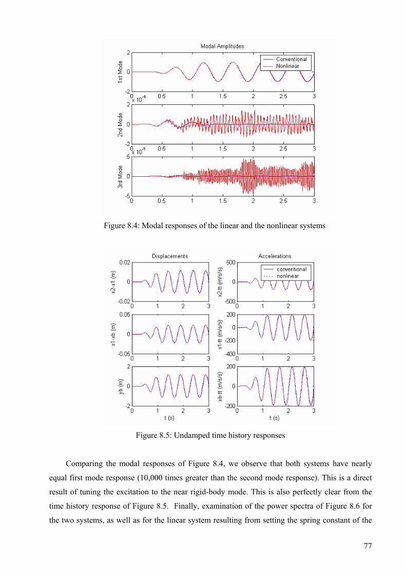
Figure 8.4: Modal responses of the linear and the nonlinear systems
Figure 8.5: Undamped time history responses
Comparing the modal responses of Figure 8.4, we observe that both systems have nearly
equal first mode response (10,000 times greater than the second mode response). This is a direct
result of tuning the excitation to the near rigid-body mode. This is also perfectly clear from the
time history response of Figure 8.5. Finally, examination of the power spectra of Figure 8.6 for
the two systems, as well as for the linear system resulting from setting the spring constant of the
77
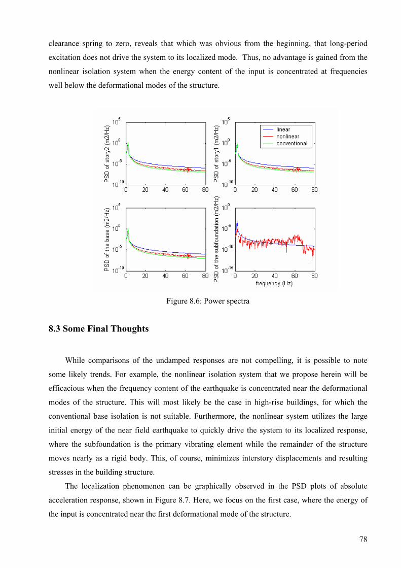
clearance spring to zero, reveals that which was obvious from the beginning, that long-period
excitation does not drive the system to its localized mode. Thus, no advantage is gained from the
nonlinear isolation system when the energy content of the input is concentrated at frequencies
well below the deformational modes of the structure.
Figure 8.6: Power spectra
8.3 Some Final Thoughts
While comparisons of the undamped responses are not compelling, it is possible to note
some likely trends. For example, the nonlinear isolation system that we propose herein will be
efficacious when the frequency content of the earthquake is concentrated near the deformational
modes of the structure. This will most likely be the case in high-rise buildings, for which the
conventional base isolation is not suitable. Furthermore, the nonlinear system utilizes the large
initial energy of the near field earthquake to quickly drive the system to its localized response,
where the subfoundation is the primary vibrating element while the remainder of the structure
moves nearly as a rigid body. This, of course, minimizes interstory displacements and resulting
stresses in the building structure.
The localization phenomenon can be graphically observed in the PSD plots of absolute
acceleration response, shown in Figure 8.7. Here, we focus on the first case, where the energy of
the input is concentrated near the first deformational mode of the structure.
78

Figure 8.7: Power spectra of absolute acceleration
Linear Nonlinear Conventional
Examination of the relative magnitudes of these spectra at the 37 Hz peak reveals the localization,
with the response of the subfoundation being orders of magnitude greater than that of the
remaining degrees of freedom. This is sharp contrast to the peak near 20 Hz, which represents a
perturbation to the linear mode and is localized to the structure and not the subfoundation.
The fundamental issue, then, is, can sufficient input energy be shifted from lower modes,
especially the near rigid-body mode, to the higher mode, localized to the subfoundation, to
significantly affect the overall response of the primary structure to the point where the new
isolation system outperforms the conventional system. The results of this brief study are
inconclusive in this regard.
79

Chapter 9: Conclusions and Recommendations for Further Study
In this thesis, a novel seismic base isolation concept has been introduced which makes use of
internal resonance and nonlinear localization to confine seismic energy to a nonstructural element,
the subfoundation, which is a noncritical part of the overall system. We have shown that, with
proper tuning, any deformational mode of the primary structure can be suppressed, with resulting
reductions in response. When compared with a nearly identical system without the additional
clearance spring (thus making the system linear), the nonlinear system performs well. The
response of the first deformational mode of the structure is almost fully suppressed, and system
response to the full-sine velocity pulse, the historic Erzincan earthquake, and the He model of the
Erzincan earthquake showed peak reductions in the interstory displacements of up to 61% and in
the absolute accelerations of up to 65%.
The potential advantages of such a system are many: First, the additional stage required, the
subfoundation, serves no purpose other than as a tuning mass. Thus, it can be fabricated
inexpensively and is not weight critical. Second, a clearance spring not only is easy to implement
but also can be specified during the design and construction stage. Thus, this simple additional
step can provide the needed strong nonlinearity. Third, this system can suppress the response of
any individual deformational mode and provide relatively broad-frequency protection. It is
similarly efficient for acceleration and displacement inputs, as well. Fourth, as stated in this
thesis, the working principle for this nonlinear element is well understood and, thus, its
performance can be predicted and assured. The degree of nonlinearity, damping location and
damping ratio can be specified according to the designer’s preference to achieve the desired level
of vibration reduction.
However, this manifestation of the system is not ideal in that, like a traditional base isolation
system, it cannot suppress the rigid-body mode, which overshadows performance when the
ground motion contains long-period pulses. It is also deficient in that it possesses only one
localized NNM. By adding additional nonlinear elements, one is able to induce more localized
NNMs in the system, thus enhancing its capacity to confine seismic energy in the subfoundation
and provide better isolation to the main structure. In addition, the design might be improved if the
subfoundation were designed with additional tunable degrees of freedom, if the nonlinear
elements were rearranged, if additional nonlinear damping elements were introduced, or if
damping and/or nonlinearities in the primary structure were considered.
These are likely candidates for future investigations.
80

List of References
Anand, G. V., 1972, “Normal Modes of a Coupled Nonlinear System”, International Journal of Nonlinear Mechanics, 7(1), 81-91. Anderson, P. W., 1978, “Localized Moments and Localized States”, Reviews of Modern Physics, 50(2), 191-201. Anderson, J. G., and Bertero, V., 1986, “Uncertainties in Establishing Design Earthquake”, Journal of Structural Engineering, ASCE, 113, 1709-1724. Anderson, J. G., Bodin, P., Brune, J. N., Prince, J. and Singh, S. K., 1986, “Strong Ground Motion from the Michoagan, Mexico Earthquake”, Science, 233, 1043-1049. Arnold, F. R., 1955, “Steady-State Behavior of Systems Provided With Nonlinear Dynamic Vibration Absorbers”, Journal of Applied Mechanics, 22, 487-492. Caughey, T. K. and O’Kelly, M. E. J., 1965, “Classical Normal Modes in Damped Linear Dynamic Systems”, Journal of Applied Mechanics, 32(3), pp583-588. Caughey, T. K., Vakakis, A. F., and Sivo, J., 1990, “Analytic Study of Similar Normal Modes and Their Bifurcations in a Class of Stronghly Nonlinear Dynamic Systems”, International Journal of Nonlinear Mechanics, 25(5), pp521-533. Chopra, A. K., 1995, Dynamics of Structures, Theory and Applications to Earthquake Engineering, Prentice-Hall, Inc. NJ. Crede, C. E., 1951, Vibration and Shock Isolation, Wiley and Sons, New York. Cuvalci, O., Ertas A. Ekwaro-Osive, S., and Cicek, I., 2002, “ Nonlinear Vibration Absorber for a System Under Sinusoidal and Random Excitation: Experiments”, Journal of Sound and Vibration, 249(4), 707-718. Dabney, J. B., and Harman, T. L., 1998, The Student Edition of SIMULINK: Dynamic System Simulation for MATLAB, Prentice Hall, New Jersey. Den Hartog, J. P, 1956, Mechanical Vibrations (4th edition), McGraw-Hill, New York. Der Kiureghian, A., Sackman, J. L. and Hong, K-J., 1999, “Interaction in Interconnected Electrical Substation Equipment Subjected to Earthquake Ground Motions”, Report PEER 1999/01, Pacific Earthquake Engineering Research Center, University of California, Berkeley, CA, February. Grubin, C., Monica S., 1956, “On the Theory of the Acceleration Damper”, ASME Journal of Applied Mechanics, 23, 373-378. Hall, J. F., Heaton, T. H., Halling, M. W., and Wald, D. J., 1995, “Near-Source Ground Motions and Effects on Flexible Buildings”, Earthquake Spectra, 11, 569-605. He, W., 2003, Smart Energy Dissipation Systems for Protection of Civil Infrastructures from Near-Field Earthquakes, PhD Thesis, The City University of New York, 2003.
81
He, W., and Agrawal, A. K., 2002, “A Closed-Form Approximation of Near-Fault Ground Motion Pulses for Flexible Structures”, to be submitted. Hodges, C, 1982, “Confinement of Vibration by Structural Irregularity”, Journal of Sound and Vibration, 82(3), 441-424. Iwan, W. D., and Chen, X. D., 1994, “Important Near-Field Ground Motion Data from the Landers Earthquake”, Proceedings of 10th European Conference of Earthquake Engineering, Vienna. Iwan, W. D., 1997, “Drift Spectrum: Measure of Demand for Earthquake Ground Motions”, Journal of Structural Engineering, 123(4), 397-404. Iwan, W. D., 2002, Personal communication with the author on International Conference on Advances and New Challenges in Earthquake Engineering Research, August 15-17, 2002, Harbin, China. Jiang, X., 2002, “Theoretical and Experimental Studies of Steady-State Nonlinear Localization and Energy Pumping in Systems of Coupled Oscillators”, Ph.D. Thesis, University of Illinois at Urbana-Champaign. Jones, D. I. G., Nashif A. D., and Adkins R. L., 1967, “Effect of Tuned Dampers on Vibrations of Simple Structures,” AIAA Journal, 5(2). Khachian, E., Der Kiureghian, A., and Tonoyan, A., 1998, “Dynamic Properties Of Primary-Secondary Systems”, Journal of Structural Engineering Association, Yerevan, Armenia, 7(24), 1-4 (in Armenian). Kelly, J. M., 1997, Earthquake-Resistant Design With Rubber, 2nd ed., Berlin and New York: Springer-Verlag. Kelly, J. M., Beucke, K. E., and Skinner, M. S., 1980, “Experimental Testing of a Friction Damped Aseismic Base-Isolation System with Fail-Safe Characteristics”, Report No. UCB/EERC-80/18, Earthquake Engineering Research Center, University of California, Berkley, CA, 1980. Leo, D. J., and Inman, D. J., 1999, “A Quadrative Programming Approach to the Design of Active-Passive Vibration Isolation Systems”, Journal of Sound and Vibration, 220(5), 807-825. Li, C, 2002, “Optimum Multiple Tuned Mass Dampers for Structures Under the Ground Acceleration Based on DDMF and ADMF”, Earthquake Engineering and Structural Dynamics, 31: 897-919. Liu, T. H., Marr, A., 1987, Seismic Engineering: Recent Advances in Design, Analysis, Testing and Qualification Methods, presented at the 1987 Pressure Vessels and Piping Conference, San Diego, California, June 28-July 2, 1987, PVP Series, 127, ASME, USA. Luongo, A. 1991, “On the Amplitude Modulation and Localization Phenomena in Interactive Buckling Problems”, International Journal of Solids and Structures, 27(15), 1943-1954.
82

MacKay, R. S., and Aubry, S., 1994, Proof of Existence of Breathers for Time-Reversible or Hamiltonian Networks of Weakly Coupled Oscillators, Nonlinear Systems Laboratory Preprint 20/1994, Mathematics Institute, University of Warwick, Coventry, UK. Makris, N., 1997, “Rigidity-Plasticity-Viscosity: Can Electrorheological Dampers Protect Base-Isolated Structures from Near-Source Ground Motions?” Earthquake Engineering and Structural Dynamics, 26, 571-591. Makris, N., and Chang, Shih-Po., 1998, “Effect of Damping Mechanisms on the Response of Seismically Isolated Structures”, PEER Report 1998/06, Pacific Earthquake Engineering Research Center, University of California, Berkeley, November 1998. Malhotra, P. K., 1997, “Dynamics of Seismic Impacts in Base-Isolated Buildings”, Earthquake Engineering and Structural Dynamics, 26, 797-813. Malhotra, P. K., 1999, “Response of Building to Near-Field Pulse-Like Ground Motions”, Earthquake Engineering and Structural Dynamics, 28, 1309-1326. Masri, S. F., 1973, “Steady-State Response of a Multidegree System With an Impact Damper”, ASME Journal of Applied Mechanics, 40, 127-132. McFarland, D. M., Wang, Y., Vakakis A. F., and Bergman L. A., 2002a, “A Parametric Analysis Of A Novel Shock Isolation System”, Proceedings of the 15th ASCE Engineering Mechanics Conference EM 2002, 2-5 June, 2002, Columbia University, New York, NY. CD-ROM, Paper no. 337, 8 pages. McFarland, D. M., Wang, Y., Vakakis, A. F., and Bergman, L. A., 2002b, “Model Testing of a Nonlinear Base Isolation Concept”, Proceedings of the International Conference on Advances in Building Technology, Hong Kong, 4-6 December 2002, 513-520. Meirovitch, L. I., 2001, “Description of Localized Normal Modes in the Chain of Nonlinear Coupled Oscillators Using Complex Variables”, Nonlinear Dynamics 25, 95-109. Naeim, F., and Kelly, J. M., 1999, Design of seismic isolated structures: From theory to practice, Wiley, Chichester, England. Nagarajaiah, S., and Xiaohong S., 2000, “Response of Base-Isolated USC Hospital Building in Northridge Earthquake”, Journal of Structural Engineering, 126(10), 1177-1186. Nakhta, T., 1973, Approximate Dynamic Response of Light Secondary Systems, Ph.D. Thesis, University of Illinois at Urbana-Champaign. Nashif, A. D., Jones, D. I. G., Henderson, J. P., 1985, Vibration Damping, Wiley and Sons, New York. Nayfeh, S. A., and Nayfeh, A. H., 1994, “Energy Transfer from High- to Low-Frequency Modes in a Flexible Structure via Modulation”, Journal of Vibration and Acoustics, 116, 203-207. Nayfeh, T. A., Emaci, E., and Vakakis A. F., 1997, “Application of Nonlinear Localization oo ohe Optimization of a Vibration Isolation System”, AIAA Journal, 35(8), 1378-1386.
83

Penzien, J. and Chopra, A., K., 1965, “Earthquake Responses of Appendage on a Muti-Story Building”, Proceedings of the Third World Conference on Earthquake Engineering, New Zealand. Pierre, C. and Dowell, E. H., 1987, “Localization of vibrations by Structural irregularity”, Journal of Sound and Vibration, 114(3), 549-564. Pierre, C. 1988, “Mode localization and Eigenvalue Loci Veering Phenomena in Disordered Structures”, Journal of Sound and Vibration, 126(3), 485-502. Pipes, L. A., 1953, “Analysis of a Nonlinear Dynamic Vibration Absorber”, Journal of Applied Mechanics, 20, 515-518. Rand, R. H., Pak, C. H., and Vakakis, A., F., 1992, “Bifurcation of NNMs in a Class of Two DOF Systems,” Acta Mechanics, (Suppl), 3, 129-145. Reed, F. E., 1961, “Dynamic Vibration Absorbers and Auxiliary Mass Dampers,” Shock and Vibration Handbook (eds. Harris C. M. and Crede C. E.), McGraw-Hill, New York. Roberson, R. E., 1952, “Synthesis of a Nonlinear Dynamic Vibration Absorber”, Journal of Applied Mechanics, 27, 263-268. Rosenberg, R. M., 1960, “Normal Modes of Nonlinear Dual-Mode Systems”, Journal of Applied Mechanics, 27, 263-368. Rosenberg, R. M., 1963, “The Ateb(h)-Functions and Their Properties”, Quart. Applied Mathematics, 21(1), 37-47. Rosenberg, R. M., and Kuo, J., 1964, “Nonsimiliar Normal Mode Vibrations in a Nonlinear System Having Two Degrees of Freedom”, Journal of Applied Mechanics, 9, 155-242. Ruzicka, G. C., 1981, Dynamic response of tuned secondary systems, Ph.D. Thesis, University of Illinois at Urbana-Champaign. Sadek, F., Mohraz, B, Taylor, A. W., and Chung, R. M., 1997, “A Method of Estimating the Parameters of Tuned Mass Dampers for Seismic Applications”, Earthquake Engineering and Structural Dynamics, 26: 617-635. Shaw, S., and Alsuwaiyan, A., 2000, “Torsional Vibration Reduction Using Passive Nonlinear Absorbers”, Smart Structures and Materials 2000, Damping and Isolation, Proceedings of SPIE, 388-399. Shaw, S., and Pierre, C., 1991, “Nonlinear Normal Modes and Invariant Manifolds”, Journal of Sound and Vibration, 150(1), 170-173. Shaw, S., and Pierre, C., 1993, “Normal Modes for Nonlinear Vibration Systems”, Journal of Sound and Vibration, 164(1), 85-124. Skinner, R. I., Robinson, W. H., McVerry G. H., 1993, An Introduction to Seismic Isolation, Willey, Chichester, England.
84

Somerville, P. G. and Graves, R. W., 1993, “Conditions That Give Rise to Unusually Large Long Period Ground Motions”, The Structural Design of Tall Buildings, 2, 211-232. Thomson, W. T., 1972, Theory of Vibration with Applications, Prentice-Hall, Inc., Englewood Cliffs, N. J., 1972. Tsai, H., 1997, “Dynamic Analysis of Base-Isolated Shear Beams Bumping Against Stops”, Earthquake Engineering and Structural Dynamics, 26, 515-528. Vakakis, A. F., 1990, “Analysis and Identification of Linear and Nonlinear Normal Modes in Vibrating Systems”, PhD Thesis, California Institute of Technology, Pasadena, CA. Vakakis, A. F., 1993, “ Analytic Study of Linear and Nonlinear Mode Localization”, Journal of Applied Mechanics, 60(2), 555-557. Vakakis, A. F., 2001, “Inducing Passive Nonlinear Energy Sinks in Linear Vibrating Systems”, Journal of Sound and Vibration, 123(3), 324-332. Vakakis, A. F., Manevitch, L. I., Mikhlin, Y. V., Pilipchuk, V. N., and Zevin, A. A. (1996). Normal Modes and Localization in Nonlinear Systems, John Wiley & Sons, New York. Vakakis, A. F., Kounadis, A. N. and Raftoyiannis, I. G., 1999, “Use Of Nonlinear Localization for Isolating Structures from Earthquake-Induced Motions”, Earthquake Engineering and Structural Dynamics, 28, 21-36. Villaverde, R., 1985, “Reduction in Seismic Response With Heavily-Damped Vibration Absorber”, Earthquake Engineering and Structural Dynamics, 13: 33-42 Wang, Y., McFarland, D. M., Vakakis, A. F., and Bergman, L. A., 2002, “Efficacy of a nonlinear base isolation system subjected to near-field earthquake motions”, Proceedings of International Conference on Advances and New Challenges in Earthquake Engineering Research, August 15-17, 2002, Harbin, China. Warburton, E. O., and Ayorinde, G. B., 1980, “Minimizing Structural Vibration with Absorbers”, Earthquake Engineering and Structural Dynamics, 8: 219-236. Yalla, S. K. and Kareem, A., 2000, “On the Beat Phenomenon in Coupled Systems”, 8th ASCE Conference on Probablistic Mechanics and Structural Reliability, PMC2000-238. Yokomichi, I., Araki, Y., Jinnouchi, Y., Inoue, J., 1996, “Impact Damper With Granular Materials for Multibody System”, Journal of Pressure Vessel Technology, 118, 95-103.
85

Appendix A Simulink Models: Nonlinear Base Isolation System
Simulink model of the 4DOF nonlinear base isolation system
86

Subsystem model of the superstructure
87

Subsystem model of the isolation system
88

Appendix B Matlab Code: Main Program VERBOSE = 0; path(path, 'F:/earthquakes/erzican') load Erz_ns.mat; %%%%%%%%%%%%%%%%%%%%%%%%%%%%%%%%%%%%% %% MDOF system (superstructure) %%%%%%%%%%%%%%%%%%%%%%%%%%%%%%%%%%%%% zeta_ss = 0.00; zeta_b = 0.00; zeta_c = 0.00; %% Undamped %% Frequency of first mode of superstructure (building) with base fixed f_ss_1 = 13.012; w_ss_1 = 2.0 * pi * f_ss_1; T_ss_1 = 1.0 / f_ss_1; %% First story m1 = 0.2; k1 = 0.5 * (3.0 + sqrt(5.0)) * m1 * w_ss_1^2; %% Second story m2 = m1; k2 = k1; %% Superstructure matrices m_ss = diag([m1, m2]); k_ss = [[k1 + k2, -k2], [-k2, k2]]; wn_ss = sqrt(eig(k_ss, m_ss)); fn_ss = wn_ss ./ (2.0 * pi); Tn_ss = 1.0 ./ fn_ss; [mode_u, lamda_u] = eig(k_ss, m_ss); M_U = mode_u' * m_ss * mode_u; K_U = mode_u * k_ss * mode_u'; beta = 2* zeta_ss/wn_ss(1); c_ss = beta* k_ss; c2 = c_ss(2,2); c1 = c_ss(1,1) - c_ss(2,2); if VERBOSE fprintf('\nSuperstructure physical parameters:\n') m1 m2 c1 c2 k1 k2 fprintf('\nNatural frequencies of 2-DOF superstructure with base fixed:\n') wn_ss fn_ss Tn_ss End %%%%%%%%%%%%%%%%%%%%%%%%%%%%%%%%%%%%% %% Ground shock %%%%%%%%%%%%%%%%%%%%%%%%%%%%%%%%%%%%%
89

global vpulse Vg Tg vpulse = 'typeB'; % The shock pulse is a complete wave Tg = 0.052 Vg = 9.81 / (2* pi/Tg); if VERBOSE if isglobal(pulseshape) fprintf('\nThe variables\n') pulseshape Ag Tg fprintf('have been declared global.\n') end vpulse Vg Tg end t0 = 0.0; tf = 3; timestep = 0.00025; simoptions = simset('FixedStep', timestep); simoptions = simset(simoptions, 'Solver', 'ode4'); %%%%%%%%%%%%%%%%%%%%%%%%%%%%%%%%%%%% %% Unisolated system %%%%%%%%%%%%%%%%%%%%%%%%%%%%%%%%%%%% n = 2; d_ss = [[k1, c1], [0, 0]]; A1_ss = [[c2, m2], [m2, 0]]; A2_ss = [[k2, 0], [0, -m2]]; B1_ss(1:2,1:2) = d_ss; A_ss = -inv(A1_ss) * A2_ss; B_ss = inv(A1_ss) * B1_ss; C_ss = eye(2*n-2); D_ss = zeros(2*n-2, 2); mb = m1; cb = c1; kb = k1; m1_disp_index = 1; m1_vel_index = n; sim('conventional_vp', [], simoptions); yb_u = yb_ss; ys_u = zs_ss + yb_ss; xs_u_tt = xs_ss_tt; xb_u_tt = xb_ss_tt; %%%%%%%%%%%%%%%%%%%%%%%%%%%%%%%%%%%%% %% Traditional Isolation System %%%%%%%%%%%%%%%%%%%%%%%%%%%%%%%%%%%%% n = 3; mb = 0.3; kb = k1 / 30.0; m_ssb = diag([mb, m1, m2]);
90

k_ssb = [[k1 + kb, -k1, 0.0], [-k1, k1 + k2, -k2], [0.0, -k2, k2]]; wn_ssb = sqrt(eig(k_ssb, m_ssb)); fn_ssb = wn_ssb./ (2.0 * pi); Tn_ssb = 1.0 ./ fn_ssb; [mode_b, lamda_b] = eig(k_ssb, m_ssb); M_C = mode_b' * m_ssb * mode_b; K_C = mode_b' * k_ssb * mode_b; wb = sqrt(kb /(m1+ m2+ mb)); cb = 2* zeta_b* wb* (m1+ m2+ mb); c_b(2:3,2:3) = c_ss; c_b(1,2)= -c1; c_b(2,1)= -c1; c_b(1,1)= c1 + cb; c = mode_b'* c_b* mode_b; for i = 1:3 zeta_ssb(i) = c(i,i)/ (2* M_C(i,i) * wn_ssb(i)); end A1_ss = [[c_ss, m_ss], [m_ss, zeros(size(m_ss))]]; A2_ss = [[k_ss, zeros(size(m_ss))], [zeros(size(m_ss)), -m_ss]]; B1_ss(1:2,1:2) = d_ss; B1_ss(3:4,1:2) = zeros(2,2); A_ss = -inv(A1_ss) * A2_ss; B_ss = inv(A1_ss) * B1_ss; C_ss = eye(2*n-2); D_ss = zeros(2*n-2, 2); m1_disp_index = 1; m1_vel_index = n; if VERBOSE mb kb cb wn_ssb fn_ssb Tn_ssb end sim('conventional_vp', [], simoptions); yb_c = yb_ss; ys_c(:,1) = zs_ss(:,1) + yb_ss; ys_c(:,2) = zs_ss(:,2) + yb_ss; xs_c_tt = xs_ss_tt; xb_c_tt = xb_ss_tt; %%%%%%%%%%%%%%%%%%%%%%%%%%%%%%%%%%% %% MDOF superstructure plus base %%%%%%%%%%%%%%%%%%%%%%%%%%%%%%%%%%% %% Matrices of superstructure plus base (with rigid-body mode) mb = 0.3; kb = k1 / 25.0;
91
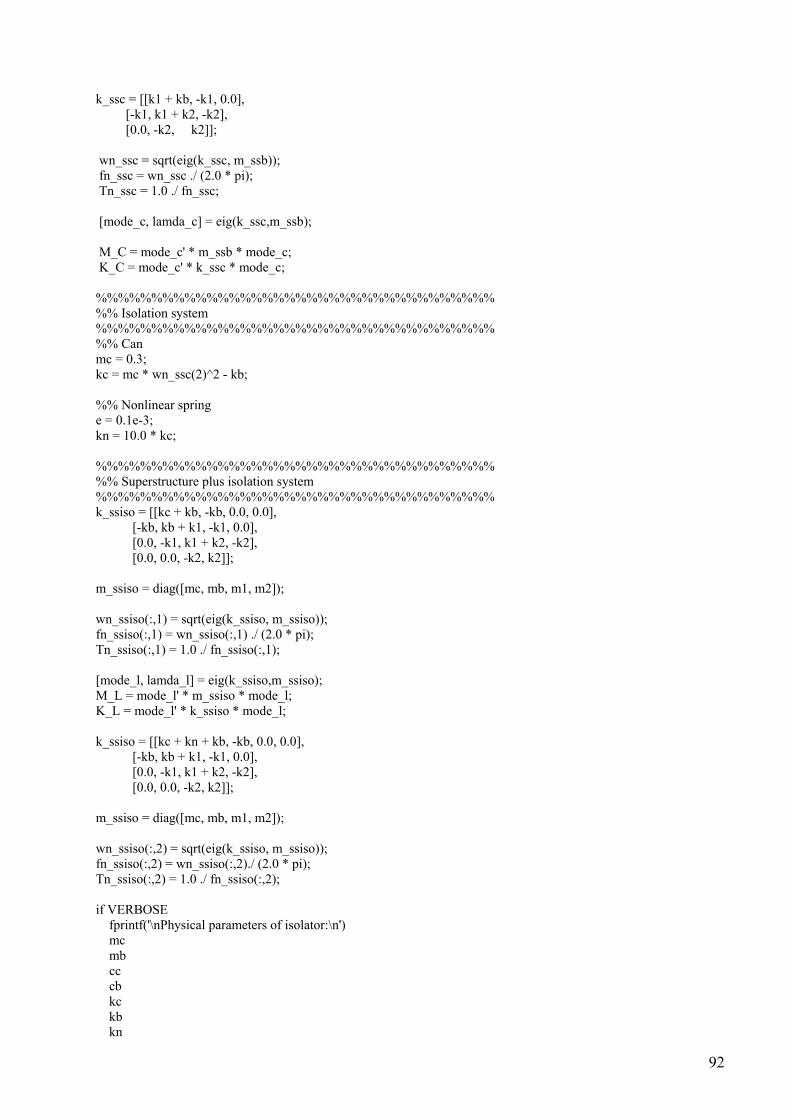
k_ssc = [[k1 + kb, -k1, 0.0], [-k1, k1 + k2, -k2], [0.0, -k2, k2]]; wn_ssc = sqrt(eig(k_ssc, m_ssb)); fn_ssc = wn_ssc ./ (2.0 * pi); Tn_ssc = 1.0 ./ fn_ssc; [mode_c, lamda_c] = eig(k_ssc,m_ssb); M_C = mode_c' * m_ssb * mode_c; K_C = mode_c' * k_ssc * mode_c; %%%%%%%%%%%%%%%%%%%%%%%%%%%%%%%%%%%% %% Isolation system %%%%%%%%%%%%%%%%%%%%%%%%%%%%%%%%%%%% %% Can mc = 0.3; kc = mc * wn_ssc(2)^2 - kb; %% Nonlinear spring e = 0.1e-3; kn = 10.0 * kc; %%%%%%%%%%%%%%%%%%%%%%%%%%%%%%%%%%%% %% Superstructure plus isolation system %%%%%%%%%%%%%%%%%%%%%%%%%%%%%%%%%%%% k_ssiso = [[kc + kb, -kb, 0.0, 0.0], [-kb, kb + k1, -k1, 0.0], [0.0, -k1, k1 + k2, -k2], [0.0, 0.0, -k2, k2]]; m_ssiso = diag([mc, mb, m1, m2]); wn_ssiso(:,1) = sqrt(eig(k_ssiso, m_ssiso)); fn_ssiso(:,1) = wn_ssiso(:,1) ./ (2.0 * pi); Tn_ssiso(:,1) = 1.0 ./ fn_ssiso(:,1); [mode_l, lamda_l] = eig(k_ssiso,m_ssiso); M_L = mode_l' * m_ssiso * mode_l; K_L = mode_l' * k_ssiso * mode_l; k_ssiso = [[kc + kn + kb, -kb, 0.0, 0.0], [-kb, kb + k1, -k1, 0.0], [0.0, -k1, k1 + k2, -k2], [0.0, 0.0, -k2, k2]]; m_ssiso = diag([mc, mb, m1, m2]); wn_ssiso(:,2) = sqrt(eig(k_ssiso, m_ssiso)); fn_ssiso(:,2) = wn_ssiso(:,2)./ (2.0 * pi); Tn_ssiso(:,2) = 1.0 ./ fn_ssiso(:,2); if VERBOSE fprintf('\nPhysical parameters of isolator:\n') mc mb cc cb kc kb kn
92

e wn_ssc fn_ssc Tn_ssc fprintf('\nModal parameters of 2-DOF superstructure plus isolation:\n') wn_ssiso fn_ssiso Tn_ssiso end wc = sqrt((kb+ kc)/mc); cc = 2* zeta_c* wc* mc; c_l(2:4,2:4) = c_b; c_l(1,2)= -cb; c_l(2,1)= -cb; c_l(1,1)= cc + cb; c = mode_l'* c_l* mode_l; for i = 1:4 zeta_ssiso(i) = c(i,i)/ (2* M_L(i,i) * wn_ssiso(i)); end %%%%%%%%%%%%%%%%%%%%%%%%%%%%%%%%%%%%%% %% Simulation %%%%%%%%%%%%%%%%%%%%%%%%%%%%%%%%%%%%%% kn = 0.0; sim('eqvp', [], simoptions); zs_lin = zs; yb_lin = yb; yc_lin = yc; ys_lin(:,1) = zs(:,1)+ yb; ys_lin(:,2) = zs(:,2)+ yb; xs_lin = xs; xb_lin = xb; xc_lin = xc; zbc_lin = yb-yc; zsb_lin = zs; zsc_lin(:,1) = zs(:,1)+ yb -yc; zsc_lin(:,2) = zs(:,2)+ yb -yc; zbc_lin = yb -yc; xs_lin_t = xs_t; xb_lin_t = xb_t; xc_lin_t = xc_t; xs_lin_tt = xs_tt; xb_lin_tt = xb_tt; xc_lin_tt = xc_tt; U_lin = U; kn = 10.0 * kc; e = max(abs(yc_lin)/10) sim('eqvp', [], simoptions); zs_n = zs; yb_n = yb; yc_n = yc; ys_n(:,1) = zs(:,1)+ yb; ys_n(:,2) = zs(:,2)+ yb; xs_n = xs;
93

xb_n = xb; xc_n = xc; zsc_n(:,1) = zs(:,1)+ yb -yc; zsc_n(:,2) = zs(:,2)+ yb -yc; zbc_n = yb -yc; yc_n = yc; xs_n_t = xs_t; xb_n_t = xb_t; xc_n_t = xc_t; xs_n_tt = xs_tt; xb_n_tt = xb_tt; xc_n_tt = xc_tt; %%%%%%%%%%%%%%%%%%%%%%%%%%%%%%%%%%%%% %% Modal Amplitudes %%%%%%%%%%%%%%%%%%%%%%%%%%%%%%%%%%%%% for i =1:length(tout) A_c(i,:) = ((mode_b' * m_ssb) *[yb_c(i),ys_c(i,1:2)]')'; end [mode, Value] = eig(k_ssb,m_ssb); IM = mode' * m_ssb; for i =1:length(tout) A_lin(i,:) = (IM*[zbc_lin(i),zsc_lin(i,1),zsc_lin(i,2)]')'; A_n(i,:) = (IM*[zbc_n(i),zsc_n(i,1),zsc_n(i,2)]')'; end %%%%%%%%%%%%%%%%%%%%%%%%%%%%%%%%%%%%% %% Power Spectral Densities %%%%%%%%%%%%%%%%%%%%%%%%%%%%%%%%%%%%% num = tf/timestep; [Pys_c(:,1),ff] = periodogram(ys_c(1:num,1),[],num,2000); [Pys_c(:,2),ff] = periodogram(ys_c(1:num,2),[],num,2000); [Pyb_c,ff] = periodogram(yb_c(1:num),[],num,2000); [Pzsc_lin(:,1),ff] = periodogram(zsc_lin(1:num,1),[],num,2000); [Pzsc_lin(:,2),ff] = periodogram(zsc_lin(1:num,2),[],num,2000); [Pzbc_lin,ff] = periodogram(zbc_lin(1:num),[],num,2000); [Pyc_lin,ff] = periodogram(yc_lin(1:num),[],num,2000); [Pzsc_n(:,1),ff] = periodogram(zsc_n(1:num,1),[],num,2000); [Pzsc_n(:,2),ff] = periodogram(zsc_n(1:num,2),[],num,2000); [Pzbc_n,ff] = periodogram(zbc_n(1:num),[],num,2000); [Pyc_n,ff] = periodogram(yc_n(1:num),[],num,2000); %%%%%%%%%%%%%%%%%%%%%%%%%%%%%%%%%%%%% %% Envelope of Absolute Control Force %%%%%%%%%%%%%%%%%%%%%%%%%%%%%%%%%%%%% [FF,Ti] = Force_Env(U,kn,tout); set(0,'DefaultAxesColorOrder',[0 0 1;1 0 0;0 1 0]) %%%%%%%%%%%%%%%%%%%%%%%%%%%%%%%%%%%%% figure(1) subplot(2,1,1) plot(tout, A_lin(:, 2),tout, A_lin(:, 3)) legend('A2','A3'); ylabel('Modal Amplitudes') title('Linear system'); subplot(2,1,2) plot(tout, A_n(:, 2),tout,A_n(:, 3)) legend('A2','A3'); ylabel('Modal Amplitudes')
94

title('Nonlinear system'); figure(3) subplot(4, 2, 1) plot(tout,zs_lin(:,2)-zs_lin(:,1),tout,zs_n(:,2)-zs_n(:,1)) ylabel('x2-x1 (m)') title('Displacements') subplot(4, 2, 3) plot(tout,zs_lin(:,1),tout,zs_n(:,1)) ylabel('x1-xb (m)') subplot(4, 2, 5) plot(tout,yb_lin,tout,yb_n) ylabel('xb-xg (m)') subplot(4, 2, 7) plot(tout,yc_lin,tout,yc_n) ylabel('xc-xg (m)') xlabel('t (s)') subplot(4, 2, 2) plot(tout,xs_lin_tt(:,2),tout,xs_n_tt(:,2)) ylabel('x2-tt (m/s/s)') %legend('linear','nonlinear'); title('Accelerations') subplot(4, 2, 4) plot(tout,xs_lin_tt(:,1),tout,xs_n_tt(:,1)) ylabel('x1-tt (m/s/s)') subplot(4, 2, 6) plot(tout,xb_lin_tt,tout,xb_n_tt) ylabel('xb-tt (m/s/s)') subplot(4, 2, 8) plot(tout,xc_lin_tt,tout,xc_n_tt) ylabel('xc-tt (m/s/s)') xlabel('t (s)') figure(4) subplot(2, 2, 1) semilogy(ff(1:240),[Pzsc_lin(1:240,2),Pzsc_n(1:240,2)]) ylabel('PSD of zc2 (m2/Hz)') subplot(2, 2, 2) semilogy(ff(1:240),[Pzsc_lin(1:240,1),Pzsc_n(1:240,1)]) legend('linear','nonlinear'); ylabel('PSD of zc1 (m2/Hz)') subplot(2, 2, 3) semilogy(ff(1:240),[Pzbc_lin(1:240),Pzbc_n(1:240)]) ylabel('PSD of zbc (m2/Hz)') subplot(2, 2, 4) semilogy(ff(1:240),[Pyc_lin(1:240),Pyc_n(1:240)]) ylabel('PSD of yc (m2/Hz)') xlabel('frequency (Hz)') figure(5) plot(tout,Fn) ylabel('F(u) (N)') xlabel('t (s)') hold on; plot(Ti,FF,'r') legend('Control Force','Force Envelope'); hold off;
95

Appendix C Matlab Code: Full-sine Ground Velocity Pulse function p = groundvel(t) global vpulse Vg Tg zeta_g switch vpulse case 'typeA' if 0.0 < t & t < Tg p = Vg * sin(pi * t / Tg); else p = 0.0; end case 'typeB' if 0.0 < t & t < Tg p = Vg * sin(2* pi * t / Tg);%+ Vg * sin(120.7095/2*t)/ 4; else p = 0.0; end case 'typeD' wd_g = 2*pi/Tg * sqrt(1 - zeta_g^2); if t >0 &t < Tg p = Vg * exp(-zeta_g *2*pi/Tg * t) * sin(wd_g * (t - 0)); else p = 0.0; end end
96

Appendix D Matlab Code: Envelope of the Control Force
function [FF,Ti] = Force_Env(U,kn,tout) count1 = 0; count2 = 0; for i = 1:length(U)-1 if U(i)==0 & U(i+1)~=0 count1 = count1 + 1; arohead(count1) = i+1; end if U(i)~= 0 & U(i+1)==0 count2 = count2 + 1; aroend(count2) = i; end end if U(length(U))~=0 count2 = count2 + 1; aroend(count2) = length(U); end for j = 1:length(arohead) for i = 1:length(U) if i>=arohead(j) & i<=aroend(j) [F,I] = max(abs(U(arohead(j):aroend(j)))); FF(j) = F * kn; Ti(j) = tout(I + arohead(j)-1); end end end
97

Appendix E Simulink Model: SDOF Oscillator
Simulink Model of SDOF oscillator used for calculating response spectra
98

Appendix F Matlab Code: Response Spectra
m = 1; zeta1 = 0.005; zeta2 = 0.02; tf = 44.905; timestep = 0.005; simoptions = simset('FixedStep', timestep); simoptions = simset(simoptions, 'Solver', 'ode4'); Tmax = 8.0; dT = 0.005; Tvec = 0.005 : dT : Tmax; for i = 3:length(Tvec) T = Tvec(i) k = (2 * pi)^2 * m / T^2; c = 2 * sqrt(k * m) * zeta1; sim('oscillator_a', [], simoptions); sd_05(i) = max(abs(disp)); sv_05(i) = max(abs(vel)); sa_05(i) = max(abs(acc)); c = 2 * sqrt(k * m) * zeta2; sim('oscillator_a', [], simoptions); sd_2(i) = max(abs(disp)); sv_2(i) = max(abs(vel)); sa_2(i) = max(abs(acc)); % c = 2 * sqrt(k * m) * zeta1; % sim('oscillator_v', [], simoptions); % sd_05(i) = max(abs(disp)); % c = 2 * sqrt(k * m) * zeta2; % sim('oscillator_v', [], simoptions); % sd_2(i) = max(abs(disp)); end figure(2) plot(Tvec,sv_2) ylabel('velocity,cm/s') xlabel('period,sec') title('Response Spectra') figure(3) plot(Tvec,sd_2) ylabel('displacement,cm') xlabel('period,sec') title('Response Spectra') load Erz_ns.mat figure(1) subplot(3,2,1) plot(1./ERZ_NS_005(11:112,2),ERZ_NS_005(11:112,6)*9.81) legend('Recorded','Approximated') ylabel('Acceleration') Title('Damping 0.5%') subplot(3,2,3) plot(11./ERZ_NS_005(11:112,2),ERZ_NS_005(11:112,4)/100) ylabel('Velocity')
99

subplot(3,2,5) plot(1./ERZ_NS_005(11:112,2),ERZ_NS_005(11:112,3)/100) ylabel('Displacement') xlabel('T (s)') subplot(3,2,2) plot(1./ERZ_NS_020(11:112,2),ERZ_NS_020(11:112,6)*9.81) legend('Recorded','Approximated') ylabel('Acceleration') Title('Damping 2%') subplot(3,2,4) plot(1./ERZ_NS_020(11:112,2),ERZ_NS_020(11:112,4)/100) ylabel('Velocity') subplot(3,2,6) plot(1./ERZ_NS_020(11:112,2),ERZ_NS_020(11:112,3)/100) ylabel('Displacement') xlabel('T (s)')
100

Appendix G Simulink Model: Conventional Isolation System
Simulink model of the 3DOF conventional base isolation system
101


![SEISMIC ROOF ISOLATION OF HALKAPINAR … · most efficient seismic isolation solution for the Halkapınar Gymnasium. In this thesis, theory of seismic isolation, ... [18] (From AASHTO](https://img.dokumen.tips/doc/110x75/5b5ba6ce7f8b9a905c8e7903/seismic-roof-isolation-of-halkapinar-most-efficient-seismic-isolation-solution.jpg)