Embed Size (px)
Citation preview

UNIVERSITY OF LJUBLJANA Faculty of Civil and Geodetic
Engineering
Institute of Structural Engineering, Earthquake Engineering and Construction IT (IKPIR)
SEISMIC ASSESSMENT OF THE SPEAR TEST STRUCTURE
Aurel STRATAN and Peter FAJFAR
IKPIR Report Ljubljana, January 2003


i
ABSTRACT
Assessment of the seismic response of a gravity load design r.c. building structure is addressed in this study. It aims at predicting the seismic performance of the structure to be tested pseudo-dynamically at ELSA in Ispra, within the EU project Seismic Performance Assessment and Rehabilitation (SPEAR), providing data needed for the experimental set-up. The test structure represents a simplification of an actual 3-storey building representative of older construction in Greece and elsewhere in the Mediterranean region, without engineered earthquake resistance. The main deficiencies of the SPEAR test structure are represented by : plain reinforcing bars; slender columns with largely spaced stirrups; column lap splices in potential plastic hinge zones; lack of shear reinforcement in beam-column joints; inadequate anchorage of stirrups, and irregular plan layout. Two 3D structural models were used, one based on one-component concentrated plasticity elements, and another one that used distributed plasticity fibre elements for columns. While the latter model is believed to estimate better the structural response in the inelastic range, the former model has the advantage of easier interpretation of results, evaluation of seismic capacity being on the safe side in comparison to the more complex fibre model. For each of the models, seismic demand was evaluated by the N2 method and by inelastic dynamic analysis. Two sets of earthquake records were used. The first one is a suite of seven recorded bidirectional ground motions, scaled to match the EC8 spectra for soil type C in the constant velocity range. A second suite of semiartificial earthquake records provided within the SPEAR project were added later to provide easier comparison of results with other project tasks. Seismic performance of the SPEAR structure was assessed for three earthquake intensity levels: 0.1g, 0.2g, and 0.3g.

ii
TABLE OF CONTENTS
ABSTRACT.............................................................................................................................................. I TABLE OF CONTENTS.......................................................................................................................... II 1. INTRODUCTION ................................................................................................................................. 1 2. THE SPEAR STRUCTURE................................................................................................................. 2 3. EARTHQUAKE RECORDS ................................................................................................................ 5 4. STRUCTURAL MODELLING AND ANALYSIS ................................................................................. 8
4.1. MATERIALS..................................................................................................................................... 8 4.2. MODELLING OF ELEMENTS............................................................................................................... 8 4.3. GEOMETRY, LOADING, AND ANALYSIS PROCEDURE.......................................................................... 14 4.4. STRUCTURAL MODELS................................................................................................................... 17
5. SEISMIC RESPONSE OF THE SPEAR STRUCTURE.................................................................... 19 5.1. DYNAMIC CHARACTERISTICS.......................................................................................................... 19 5.2. EARTHQUAKE INTENSITY LEVEL 0.2G ............................................................................................. 20
5.2.1. Pushover analysis............................................................................................................... 20 5.2.2. Dynamic analysis ................................................................................................................ 22 5.2.3. Shear capacity check.......................................................................................................... 61
5.3. EARTHQUAKE INTENSITY LEVEL 0.1G ............................................................................................. 66 5.3.1. Pushover analysis............................................................................................................... 66 5.3.2. Dynamic analysis ................................................................................................................ 67
5.4. EARTHQUAKE INTENSITY LEVEL 0.3G ............................................................................................. 75 5.4.1. Pushover analysis............................................................................................................... 75 5.4.2. Dynamic analysis ................................................................................................................ 76
5.5. DIFFERENCE BETWEEN THE RESPONSE OF ETCP AND EFCP MODELS ............................................ 89 5.6. EVALUATION OF SEISMIC CAPACITY ................................................................................................ 90
6. RESPONSE UNDER THE SPEAR SET OF ACCELEROGRAMS .................................................. 92 7. SUMMARY AND CONCLUSIONS.................................................................................................. 107 ACKNOWLEDGEMENTS ................................................................................................................... 109 REFERENCES .................................................................................................................................... 110 ANNEX I. DESCRIPTION OF THE SPEAR STRUCTURE ................................................................ 112 ANNEX II. ACCELERATION TIME-HISTORIES AND RESPONSE SPECTRA OF CONSIDERED GROUND MOTIONS........................................................................................................................... 121 ANNEX III. MOMENT-CURVATURE AND MOMENT–ROTATION IDEALISATION OF ELEMENTS FOR ONE-COMPONENT MODEL...................................................................................................... 127 ANNEX IV. DETERMINATION OF DISPLACEMENT DEMAND BY N2 METHOD........................... 141 ANNEX V. THE SPEAR SET OF ACCELEROGRAMS ..................................................................... 145

Introduction 1
1. INTRODUCTION
Reinforced concrete structures in regions of low to moderate seismicity were traditionally designed for gravity loads alone, without any seismic provisions. This category of buildings are termed gravity load designed (GLD) frames, and are characteristic for buildings designed between 1930s and 1970s (Priestley, 1997), when design codes were implemented containing seismic provisions more or less equivalent to those currently in practice. Though local design practices and codes were different in different geographical areas, this problem is common to many regions, such as USA (Kunnath et al., 1995), New Zealand (Park, 2002), and Europe (Cosenza et al., 2002, Calvi et al., 2002). The main deficiencies in reinforced concrete GLD frames are related to poor detailing and lack of capacity design, leading to reduced local and global ductility. The following are the typical features of GLD frames (Aycardi et al., 1994, Priestley, 1997, Cosenza et al., 2002): Columns are weaker than the adjacent beams, leading to a storey mechanism. Minimal transverse reinforcement in columns for shear and confinement,
particularly in the plastic hinge zones. Frequently, transverse reinforcement is anchored with 90° bends in the cover concrete. Large spacing and inadequate anchorage lead to spalling of compression concrete, buckling of longitudinal reinforcement and collapse of the plastic hinge regions.
Little or no transverse reinforcement in beam-column joints, resulting in a high potential for joint shear failure.
Discontinuous positive (bottom) beam longitudinal reinforcement in the beam-column joints.
Lap splices located in potential plastic hinge zones just above the floor slab levels.
Plain reinforcing bars for longitudinal reinforcement, that leads to early loss of bond and increases deformations in the structure.
Inclined reinforcement for shear resistance in beams, that is not effective for shear reversals.
Lack of structural regularity in plan and/or elevation, further worsening the seismic response due to torsion and storey mechanisms.
2 The SPEAR structure
2. THE SPEAR STRUCTURE
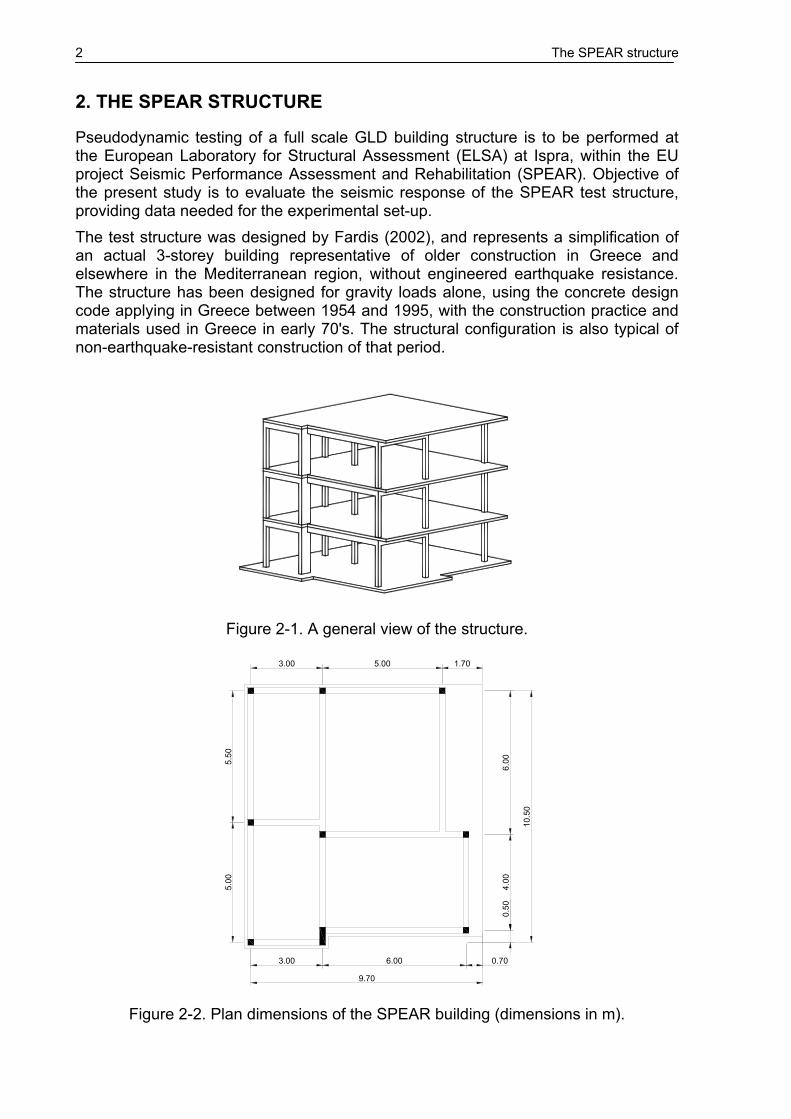
Pseudodynamic testing of a full scale GLD building structure is to be performed at the European Laboratory for Structural Assessment (ELSA) at Ispra, within the EU project Seismic Performance Assessment and Rehabilitation (SPEAR). Objective of the present study is to evaluate the seismic response of the SPEAR test structure, providing data needed for the experimental set-up. The test structure was designed by Fardis (2002), and represents a simplification of an actual 3-storey building representative of older construction in Greece and elsewhere in the Mediterranean region, without engineered earthquake resistance. The structure has been designed for gravity loads alone, using the concrete design code applying in Greece between 1954 and 1995, with the construction practice and materials used in Greece in early 70's. The structural configuration is also typical of non-earthquake-resistant construction of that period.
Figure 2-1. A general view of the structure.
10.5
0
6.00
4.00
0.50
5.50
5.00
9.70
6.003.00 0.70
5.003.00 1.70
Figure 2-2. Plan dimensions of the SPEAR building (dimensions in m).
The SPEAR structure 3
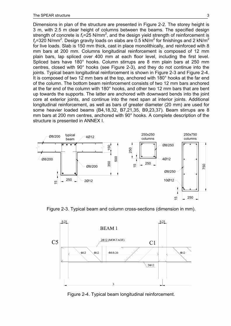
Dimensions in plan of the structure are presented in Figure 2-2. The storey height is 3 m, with 2.5 m clear height of columns between the beams. The specified design strength of concrete is fc=25 N/mm2, and the design yield strength of reinforcement is fy=320 N/mm2. Design gravity loads on slabs are 0.5 kN/m2 for finishings and 2 kN/m2 for live loads. Slab is 150 mm thick, cast in place monolithically, and reinforced with 8 mm bars at 200 mm. Columns longitudinal reinforcement is composed of 12 mm plain bars, lap spliced over 400 mm at each floor level, including the first level. Spliced bars have 180° hooks. Column stirrups are 8 mm plain bars at 250 mm centres, closed with 90° hooks (see Figure 2-3), and they do not continue into the joints. Typical beam longitudinal reinforcement is shown in Figure 2-3 and Figure 2-4. It is composed of two 12 mm bars at the top, anchored with 180° hooks at the far end of the column. The bottom beam reinforcement consists of two 12 mm bars anchored at the far end of the column with 180° hooks, and other two 12 mm bars that are bent up towards the supports. The latter are anchored with downward bends into the joint core at exterior joints, and continue into the next span at interior joints. Additional longitudinal reinforcement, as well as bars of greater diameter (20 mm) are used for some heavier loaded beams (B4,18,32, B7,21,35, B9,23,37). Beam stirrups are 8 mm bars at 200 mm centres, anchored with 90° hooks. A complete description of the structure is presented in ANNEX I.
750
250
250
250
15
15
250x250 columns
250x750 columns
4Ø12
Ø8/250
Ø8/250
10Ø12250
15
Ø8/200
2Ø12
4Ø12Ø8/200
Ø8/200
150
350 50
0
typical beam
Figure 2-3. Typical beam and column cross-sections (dimension in mm).
Figure 2-4. Typical beam longitudinal reinforcement.

4 The SPEAR structure
The main deficiencies of the SPEAR test structure could be summarised as follows: use of plain reinforcing bars slender columns (250x250), with largely spaced stirrups inclined reinforcement in beams for shear resistance and optimal distribution of
reinforcement column lap splices in potential plastic hinge zones lack of shear reinforcement in beam-column joints inadequate anchorage of stirrups (90° hooks) irregular plan layout
Influence of modelling parameters and analysis procedure on the seismic evaluation of the SPEAR structure was performed in a companion study (Stratan and Fajfar, 2002). Considerable scatter in response was obtained by considering different modelling options commonly adopted by the engineering profession for seismic analysis of r.c. frame structures. However, based on the obtained results, two structural models were identified as representing the "best estimate" of the seismic response of the SPEAR structure. Analytical modelling of critical elements (columns) was validated by correlation with experimental tests on specimens similar to the SPEAR building 250x250 columns available in literature. In the present study the structural response is assessed by nonlinear dynamic (time-history) analysis, and by the N2 method (Fajfar, 2000) based on nonlinear static (pushover) analysis. CANNY 99 computer program (Li, 2002) was used for both types of analyses.

Earthquake records 5
3. EARTHQUAKE RECORDS
Seven ground motion records from Southern Europe were selected (see Table 3-1) from the European strong motion databank (Ambraseys et al., 2000). The selection of records was based on criteria of magnitude (at least 5.8), peak ground acceleration (at least 1.5 m/s2), and conformity to the Eurocode 8 spectrum. The basic characteristics of the records are presented in Table 3-2.
Table 3-1. Earthquake records used in this study.
Earthquake name Date Station name Record
abbr. Alkion 24.02.1981 Korinthos - OTE Building AL1 Alkion 24.02.1981 Xilokastro - OTE Building AL2 Campano Lucano 23.11.1980 Calitri CA1
Kalamata 13.09.1986 Kalamata – Prefecture KA1 Kalamata 13.09.1986 Kalamata - OTE Building KA2 Montenegro 15.04.1979 Ulcinj - Hotel Albatros MO1 Montenegro 15.04.1979 Bar - Skupstina Opstine MO2
Table 3-2. Characteristics of the earthquake records.
Record Surface - wave magnitude (Ms)
Epicentral distance
Soil category PGA, m/s2 Scaling
factor AL1 6.7 20km soft soil 2.26 (X), 3.04 (Y) 1.074 AL2 6.7 19km alluvium 2.84 (X), 1.67 (Y) 0.937 CA1 6.9 16km stiff soil 1.53 (X), 1.73 (Y) 0.813 KA1 5.8 9km stiff soil 2.11 (X), 2.91 (Y) 0.791 KA2 5.8 10km stiff soil 2.35 (X), 2.67 (Y) 1.047 MO1 7.0 21km Rock 1.78 (X), 2.20 (Y) 0.991 MO2 7.0 16km stiff soil 3.68 (X), 3.56 (Y) 0.388
Scaling of the ground motion records was performed in order to bring them to the same level of seismic intensity. Eurocode 8 (2002) acceleration elastic response spectrum was used as the target spectrum (PGA=0.2g, soil parameter S=1, TB=0.2s, TC=0.6s, TD=2.0s, 5% damping). Three-dimensional nonlinear dynamic analysis requires bidirectional records (vertical component was ignored in this study). It was decided not to alter the ratio of intensities between the two components. Therefore, the procedure suggested in FEMA 356, (2000) was used here. It involves construction of the Square Root of Sum of Squares (SRSS) spectrum from the two horizontal components of each record, and applying the scaling procedure to the SRSS target spectrum (one-directional EC8 spectrum times 2 ). Scaling procedure was applied for each record separately, by minimizing the error function. The error function was defined as the difference between the areas under the SRSS spectrum of a record and the SRSS of the target spectrum in the period range between TC and TD. The fundamental period of vibration of the structure is situated in this range. The mean of SRSS spectra of scaled records, the mean plus/minus standard deviation, and the target SRSS spectrum are shown in Figure 3-1.

6 Earthquake records
0 1 2 3 40
2
4
6
8
10
12
T, s
SA
, m/s
2
SRSS OF SCALED RECORDS
EC8MEANMEAN + STDMEAN − STD
Figure 3-1. Mean of the Square Root of Sum of Squares (SRSS) of scaled records
and the target EC8 spectrum.
0 1 2 3 40
1
2
3
4
5
6
7
8
T, s
SA
, m/s
2
X COMPONENTS SCALED
EC8MEANMEAN + STDMEAN − STD
Figure 3-2. Mean of the X components of scaled records and the target EC8
spectrum. The applied scaling procedure assures a uniform intensity of seismic input near the fundamental period of the structure, and enables a direct comparison of the results from nonlinear dynamic analyses to the simplified pushover (N2) method. Mean of individual X and Y components of the records are presented in Figure 3-2 and Figure 3-3. A reasonable fit to the target EC8 spectrum could be observed in this case also. Acceleration time histories of the scaled records, as well as elastic response spectra of individual scaled and unscaled records are presented in ANNEX II.

Earthquake records 7
0 1 2 3 40
2
4
6
8
10
T, s
SA
, m/s
2
Y COMPONENTS SCALED
EC8MEANMEAN + STDMEAN − STD
Figure 3-3. Mean of the Y components of scaled records and the target EC8
spectrum.

8 Structural modelling and analysis
4. STRUCTURAL MODELLING AND ANALYSIS
4.1. Materials
Expected material strengths were estimated by Priestley, (1997), see Table 4-1. Concrete was considered unconfined for establishing the stress-strain relationship, as suggested by Priestley (1997) when the following conditions govern: stirrups ends not bent back into the core, and spacing of stirrups in the potential plastic hinge is such that: s≥d/2 or s≥16dbl
where s is the stirrups spacing, d is the effective depth of the cross section, and dbl is the diameter of the longitudinal reinforcement. For the SPEAR building, these requirements imply unconfined conditions for both beams and columns. Strain hardening was considered for steel and degradation for concrete in compression. The softening branch of concrete stress-strain relationship is the one of Kent & Park, described in Penelis and Kappos (1997), see Figure 4-1. Ultimate steel strain was considered 0.05, according to the FEMA 356 recommendations.
Table 4-1. Material characteristics.
Concrete compression strength (fc) 37.5 N/mm2
(1.5 fck)
Steel yield strength (fy) 352 N/mm2
(1.1 fyk) Ultimate concrete strain 0.0037 (at 0.2fc) Ultimate steel strain 0.05
where: fck – concrete characteristic (nominal) compression strength; fyk – steel characteristic yield strength.
0
100
200
300
400
500
0 0.02 0.04 0.06
STRAIN
STR
ESS,
N/m
m2
0.0
5.0
10.0
15.0
20.0
25.0
30.0
35.0
40.0
0 0.002 0.004 0.006
STRAIN
STR
ESS,
N/m
m2
CoreCover
Figure 4-1. Stress-strain models for steel and concrete.
4.2. Modelling of elements
Inelastic flexural behaviour of elements was considered by one-component lumped plasticity model and distributed plasticity fibre model. Shear and torsional behaviour were assumed elastic in all cases. In the case of the one-component model, all inelastic deformations are assumed concentrated at element ends (lumped plasticity model). Trilinear moment-rotation

Structural modelling and analysis 9
envelope is used, with Takeda hysteretic rules. The CANNY implementation of the model is strictly correct only for elements in double curvature bending with the inflexion point located at the mid length of the member, and it does not account for axial force-moment (M-N) and biaxial moment (M-M) interaction. A standard moment-curvature analysis was carried out for each element. For columns, axial force corresponding to gravitational loading was considered. Cracking curvature cφ was defined as the one corresponding to the attainment of the lower cracking moment Mc in the cross section. The yield curvature yφ and moment My were determined by a numerical procedure based on a significant reduction of the slope to the moment-curvature curve. The ultimate curvature uφ was determined at the attainment of ultimate strains in concrete or steel. The equivalent plastic hinge length was determined according to Paulay and Priestley, 1992 as:
0.08 0.022p b yL L d f= ⋅ + ⋅ ⋅ (4-1)
where L is the shear span of the member (assumed half the clear span for most of the members), db is the diameter of the longitudinal reinforcement, and fy is the yield strength of the reinforcement.
M
φc
c yM
φc
cM
φy
MuMcMy
L L
φc
yφ
Lp
uφ
Figure 4-2. Curvature distribution along the shear span
for trilinear moment-curvature idealisation. Then, the moment-rotation relationship is obtained by integrating the curvature distribution along the element length (see Figure 4-2):
/ 3c c Lθ φ= ⋅ (4-2)
1 1 26
c c cy c y
y y y
M M MLM M M
θ φ φ
= ⋅ ⋅ + + ⋅ − ⋅ + (4-3)
( ) ( )θ θ φ φ
⋅ − ⋅= + −
0.5p pu y u y
L L LL
(4-4)
where cθ is the rotation at cracking, yθ is the yield rotation and uθ is the ultimate rotation. The distributed plasticity model is based on discretisation of cross-sections at the element ends into a number of fibres (see Figure 4-3) and the assumption of linear variation of curvature along the element. Material stress-strain curves presented in Figure 4-1 were used for steel and concrete fibres. The fibre model accounts naturally for the interaction of biaxial moments and axial force.

10 Structural modelling and analysis
2502
2
4
750
4
250
37
35
33
31
29
27
25
23
12
10
24
2
19
15
11
822
28
32
36
18
27
31
35
14
26
30
3420 33
16 29
12 25
106
250
X
3882818079
3678777675
3474737271
3270696867
3066656463
2862616059
2658575655
24545352
9
X
51
16 18 20 22 146
49
47
45
43
41
39
11
8
31
3
17
2340
21
39
17
38
135 9
24 37
Y5
50106105104103
4810210110099
4698979695
4494939291
4290898887
4086858483
7
3
Y
15 17 19 21 135
1
13
4
Figure 4-3. Discretisation of column cross-sections for fibre element.
Insufficient anchorage of reinforcement was accounted for by the procedure suggested in FEMA356 (2000), by reducing the yield strength of bars proportionally to the ratio of available anchorage length to the one required for full anchorage:
,,
,
b avy eq y
b req
lf f
l= ⋅ (4-5)
where fy is the bar yield strength, lb,av is the available anchorage length, lb,req is the anchorage length required for full bar anchorage. The bar length required for full anchorage was deduced from the provisions of Eurocode 2 (1999 version, as the last draft do not contain provisions for plain bars), considering good bond conditions (horizontal bars in lower half of the member), and sufficient cover to prevent splitting failure (transverse beams present in most cases). For the sake of simplicity and considering that the bottom bar capacity is critical, no distinction was made between bottom and top bars required anchorage length. The bond stress of plain bars is given by:
0.36b cf f= ⋅ (4-6)
The required anchorage length was determined as:
0.74
ybb
b
fdlf
= ⋅ ⋅ (4-7)
where db is the bar diameter, and 0.7 is a coefficient accounting for the presence of hook.
Structural modelling and analysis 11
Table 4-2. Equivalent bar yield strength for insufficient anchorage.
db, mm lb,av, mm lb,req, mm fy,eq, N/mm2 fy,eq/fy 12 220 336 231 0.66 20 220 560 138 0.39
The required anchorage length and the equivalent yield strength of beam bars with insufficient anchorage are presented in Table 4-2. They apply to bottom beam bars and to beam "montage" bars at the top. Column splices are 400 mm length and would qualify as fully anchored. Their modelling was not explicitly accounted for. The procedure adopted here to account for anchorage failure is rather simplistic and do not reflect all the aspects of this phenomenon. However, very limited information is available in literature on the behaviour of reinforced concrete elements with this particular detailing (hooked plain bars). Therefore, the simple procedure described above was used for all the structural models considered in this study. Effective widths of beams were determined according to Paulay and Priestley, 1992, and are presented in Table 4-3 for first storey beams, together with the effective longitudinal reinforcement. Ends i and j are assigned in the positive directions of the X and Y axes. Upper storey beams are identical to the corresponding elements in the first storey.
Table 4-3. Beam effective width and reinforcement.
effective width, mm
bottom reinforcement
top web reinforcement
top slab reinforcement
B1i, B5i, B5j 750 2φ12 ins 2φ12 ins
2φ12 full 3φ8
B1j 750 2φ12 ins 2φ12 ins 4φ12 full 8φ8
B2i 1250 2φ12 ins 2φ12 ins 4φ12 full 13φ8
B2j 1250 2φ12 ins 2φ12 ins 2φ12 full 15φ8
B3i, B3j 1500 2φ12 ins 2φ12 ins 2φ12 full 8φ8
B4i 1750 3φ20 ins 2φ12 ins 4φ20 full 14φ8
B4j 1750 5φ20 ins 2φ12 full 15φ8
B6ij 1500 2φ12 ins 2φ12 ins 2φ12 full 11φ8
B7i 3000 2φ12 ins 2φ12 ins 3φ20 full 25φ8
B7j 1500 2φ12 ins 2φ12 ins 3φ20 full 7φ8
B8i, B8j 1250 2φ12 ins 2φ12 ins 2φ12 full 6φ8
B9i 1750 2φ20 full 4φ12 full 1φ20 full 13φ8
B9j 2000 2φ20 ins 2φ12 ins 2φ20 full 9φ8
B10i 1250 2φ12 ins 4φ12 full 6φ8

12 Structural modelling and analysis
B10j 1250 2φ12 ins 2φ12 ins 2φ12 full 2φ20 full
8φ8
B11i 1375 2φ12 ins 2φ12 ins 4φ12 full 9φ8
B11j, B12i 750 2φ12 ins 2φ12 ins
2φ12 full 2φ8
B12j 1250 2φ12 ins 2φ12 ins 4φ12 full 9φ8
B13i 1750 3φ20 full 2φ12 full 1φ20 full 18φ8
B13j 1125 3φ20 ins 2φ12 ins 3φ20 full 9φ8
B14i, B14j 1750 2φ20 ins
2φ12 ins 2φ12 full 2φ20 full
19φ8
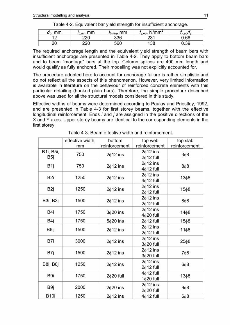
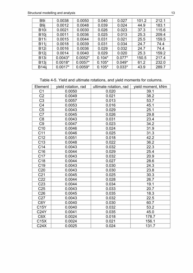
Note: ins – insufficient anchorage (lb=220mm), full – full anchorage provided. The yield and ultimate rotations (or curvatures for the B13 and B14 beams), and yield moments for the one-component modelling of the SPEAR building members are presented in Table 4-4 and Table 4-5, and graphically in ANNEX III. It can be observed that beams moment capacity is much higher under negative bending (top reinforcement in tension). Positive flexural capacity of beams is generally lower then or close to the flexural capacity of 250x250 columns. Rotation capacity of columns is strongly dependent on the axial force and is lower for first storey columns subjected to higher axial compression. A comparison of the above analytical plastic rotation capacities to FEMA356 empirical predictions (tabulated values based on detailing and magnitude of axial and shear forces) show that the latter are more conservative for columns, but similar for beams. Even higher rotations at element failure are predicted by the distributed plasticity fibre model for columns (Stratan and Fajfar, 2002).
Table 4-4. Yield and ultimate rotations, and yield moments for beams.
yield rotation, rad (curvature*, 1/m)
ultimate rotation, rad(curvature*, 1/m) yield moment, kNm Element
POS NEG POS NEG POS NEG B1i, B5ij 0.0010 0.0022 0.021 0.022 24.7 82.1
B1j 0.0010 0.0024 0.021 0.014 24.7 151.5 B2i 0.0014 0.0041 0.029 0.017 25.3 187.0 B2j 0.0014 0.0041 0.029 0.018 25.3 171.7 B3i 0.0008 0.0023 0.021 0.018 25.6 120.1 B3j 0.0008 0.0023 0.021 0.018 25.6 120.1 B4i 0.0014 0.0056 0.039 0.016 63.0 310.5 B4j 0.0042 0.0045 0.036 0.041 248.2 152.7 B6ij 0.0016 0.0047 0.033 0.025 25.7 142.3 B7i 0.0010 0.0059 0.038 0.014 27.3 336.6 B7j 0.0016 0.0054 0.039 0.020 25.6 214.1 B8i 0.0011 0.0030 0.025 0.025 25.4 105.0 B8j 0.0011 0.0030 0.025 0.025 25.4 105.0
Structural modelling and analysis 13
B9i 0.0038 0.0050 0.040 0.027 101.2 212.1 B9j 0.0012 0.0048 0.039 0.024 44.9 183.1 B10i 0.0021 0.0030 0.026 0.023 37.3 115.6 B10j 0.0011 0.0036 0.025 0.013 25.3 209.4 B11i 0.0015 0.0044 0.031 0.021 25.5 159.5 B11j 0.0018 0.0039 0.031 0.034 24.7 74.4 B12i 0.0016 0.0036 0.029 0.032 24.7 74.4 B12j 0.0014 0.0040 0.029 0.020 25.3 159.2 B13i 0.0043* 0.0052* 0.104* 0.077* 150.5 217.4 B13j 0.0018* 0.0057* 0.105* 0.049* 61.2 232.0 B14ij 0.0017* 0.0059* 0.105* 0.033* 43.9 289.7
Table 4-5. Yield and ultimate rotations, and yield moments for columns.
Element yield rotation, rad ultimate rotation, rad yield moment, kNm C1 0.0050 0.020 39.1 C2 0.0049 0.021 38.2 C3 0.0057 0.013 53.7 C4 0.0053 0.016 45.1 C5 0.0043 0.029 25.1 C7 0.0045 0.026 29.8 C8 0.0043 0.031 23.4 C9 0.0047 0.023 34.2 C10 0.0046 0.024 31.9 C11 0.0046 0.025 31.3 C12 0.0051 0.018 42.2 C13 0.0048 0.022 36.2 C14 0.0043 0.032 22.3 C16 0.0044 0.029 25.4 C17 0.0043 0.032 20.9 C18 0.0044 0.027 28.6 C19 0.0043 0.030 24.3 C20 0.0043 0.030 23.8 C21 0.0045 0.025 30.3 C22 0.0044 0.028 26.7 C23 0.0044 0.034 19.1 C25 0.0043 0.033 20.7 C26 0.0045 0.035 18.3 C27 0.0043 0.032 22.5 C6Y 0.0040 0.030 60.7
C15Y 0.0040 0.032 53.2 C24Y 0.0041 0.035 45.0 C6X 0.0024 0.018 178.7
C15X 0.0024 0.021 156.1 C24X 0.0025 0.024 131.7
14 Structural modelling and analysis
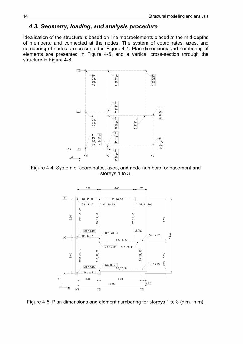
4.3. Geometry, loading, and analysis procedure
Idealisation of the structure is based on line macroelements placed at the mid-depths of members, and connected at the nodes. The system of coordinates, axes, and numbering of nodes are presented in Figure 4-4. Plan dimensions and numbering of elements are presented in Figure 4-5, and a vertical cross-section through the structure in Figure 4-6.
X2
X1
X3
Y1 Y2 Y3
10, 23, 36, 49
8, 21, 34, 47
1, 13, 26, 39
2, 14, 27, 40
3, 15, 28, 41
4, 16, 29, 42
6, 18, 31, 44
9, 22, 35, 48
11, 24, 37, 50
5, 17, 30, 43
7, 20, 33, 46-,
19, 32, 45
12, 25, 38, 51
Z
Y
X Figure 4-4. System of coordinates, axes, and node numbers for basement and
storeys 1 to 3.
3.00 6.00
5.00
5.50
0.50
4.00
6.00
3.00 5.00 1.70
B1, 15, 29
C5, 14, 23 C1, 10, 19 C2, 11, 20
C9, 18, 27
C3, 12, 21
C4, 13, 22
C7, 16, 25C6, 15, 24C8, 17, 26
B2, 16, 30
B3, 17, 31B4, 18, 32
B6, 20, 34B5, 19, 33
B11
, 25,
39
B12
, 26,
40
B9,
23,
37
B7,
21,
35
B8,
22,
36
B10
, 24,
38
B14, 28, 42
B13, 27, 41
0.70
1.00
10.5
0
9.70
X3
X2
X1
Y1 Y2 Y3Z
Y
X
Figure 4-5. Plan dimensions and element numbering for storeys 1 to 3 (dim. in m).

Structural modelling and analysis 15
6.003.00
Y1 Y2 Y3
2.50
0.50
2.50
0.50
2.50
0.50
2.75
3.00
3.00
Z
X
Figure 4-6. Vertical cross-section through the structure (dimensions in m).
Live loads and dead loads from partitions were assumed applied to all the three stories. Self-weight of r.c. members and the slab was computed considering a specific weight of concrete of 2500 kg/m3. Gravitational loading for the seismic load combinations was assumed according to Eurocode 8 and Eurocode 1 as
2 0.3iG Q G Qψ+ ⋅ = + ⋅ , where G is the permanent load (finishings and self-weight of r.c. slab and members), and Q is the live load. The tributary gravitational load was assigned to beams, and assumed uniformly distributed on the beam clear span (between the column faces). Rigid diaphragm action was considered at the floor levels, due to monolithic r.c. slab. Masses were determined according to the EC8 as corresponding to the loads from the 2iG Qϕ ψ+ ⋅ ⋅ combination, where ϕ=0.8 for stories 1-2 and 1.0 for roof. Translational masses (M) and mass moment of inertia (MMI) were applied at the centre of mass (CM) of each floor (see Table 4-6). Table 4-6. Translational masses and mass moment of inertia of the SPEAR building.
Centre of Mass Mass Mass Moment of Inertia
FLOOR 1&2 X = 4.53 m Y = 5.29 m 65.5 t 1254 tm2
ROOF X = 4.57 m Y = 5.33 m 64.1 t 1196 tm2
Centre of stiffness for each floor, determined according to EC8 as the centre of stiffness of column moment of inertia is presented in Figure 4-7. Torsional characteristics used for classification of building regularity in plan in EC8 are presented in Figure 4-5, where e0x, e0y are eccentricities measured along the X and Y axes respectively, rx, ry are torsional radii, and ls is the radius of gyration of a floor in plan. The following conditions need to be verified for each principal direction to consider the structure as regular in plan:
0 0.3x xe r≤ ⋅ , 0 0.3y ye r≤ ⋅ (4-8)

16 Structural modelling and analysis
x sr l≥ , y sr l≥ (4-9)
Thus, the SPEAR structure is classified as irregular in plan according to EC8 provisions. Torsional eccentricities are larger in the Y direction.
Table 4-7. Torsional characteristics of the SPEAR building.
e0x, m e0y, m rx, m ry, m ls, m 0.3rx 0.3ry FLOOR 1&2 1.302 1.037 1.44 2.57 4.38 0.43 0.77
ROOF 1.338 1.081 1.44 2.57 4.32 0.43 0.77
5.29
4.53 4.57
5.33
CMCM
CS1.30
1.04
FLOORS 1&2
3.23
4.25
4.25
CS
3.23
1.34
1.08
ROOF
Z X
Y Y
Z X
Figure 4-7. Centre of mass and elastic centre of stiffness of the SPEAR building.
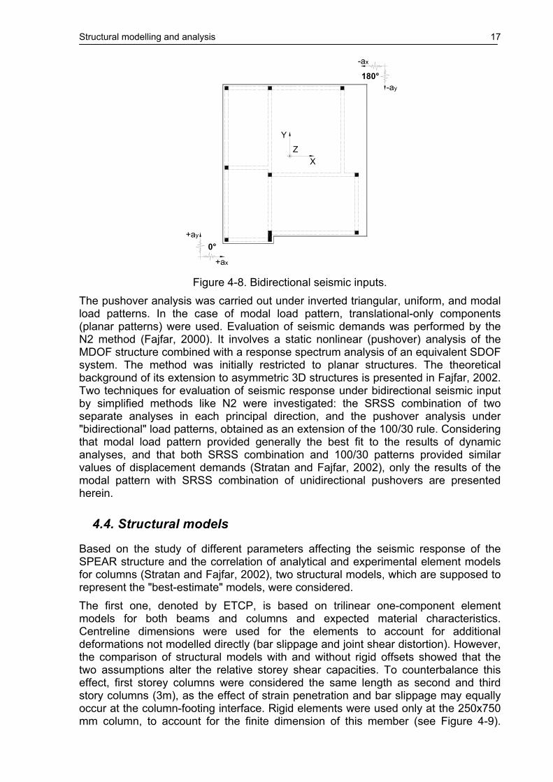
Seismic response of the SPEAR structure was evaluated by two analysis procedures: nonlinear dynamic (time-history) and nonlinear static (pushover). Second order (P-delta) effects were not considered in the analysis due to current program limitation. In the case of time-history analysis, 5% Rayleigh damping was used, for the first two modes of vibration. The stiffness-proportional damping was applied to the instantaneous stiffness matrix. Time-history analyses were performed under bidirectional pairs accelerograms, applied at 0° and 180° (see Figure 4-8), and the maximum response quantities were obtained as the maximum of the two analyses runs, separately for positive and negative values. This procedure was adopted due to unsymmetrical properties at both the element (beam moment capacities) and structural (base shear in the Y direction) levels. Additional discussion of the procedure is presented in Stratan and Fajfar, 2002. Three earthquake intensity levels were used, corresponding to 0.1g, 0.2g, and 0.3g peak ground acceleration (PGA) of the target spectrum. The PGA value includes the code soil coefficient, i.e. it is represent the peak acceleration on top of the soil layer.
Structural modelling and analysis 17
0°
+ax
+ay
Z
Y
X
-ax
180°-ay
Figure 4-8. Bidirectional seismic inputs.
The pushover analysis was carried out under inverted triangular, uniform, and modal load patterns. In the case of modal load pattern, translational-only components (planar patterns) were used. Evaluation of seismic demands was performed by the N2 method (Fajfar, 2000). It involves a static nonlinear (pushover) analysis of the MDOF structure combined with a response spectrum analysis of an equivalent SDOF system. The method was initially restricted to planar structures. The theoretical background of its extension to asymmetric 3D structures is presented in Fajfar, 2002. Two techniques for evaluation of seismic response under bidirectional seismic input by simplified methods like N2 were investigated: the SRSS combination of two separate analyses in each principal direction, and the pushover analysis under "bidirectional" load patterns, obtained as an extension of the 100/30 rule. Considering that modal load pattern provided generally the best fit to the results of dynamic analyses, and that both SRSS combination and 100/30 patterns provided similar values of displacement demands (Stratan and Fajfar, 2002), only the results of the modal pattern with SRSS combination of unidirectional pushovers are presented herein.
4.4. Structural models
Based on the study of different parameters affecting the seismic response of the SPEAR structure and the correlation of analytical and experimental element models for columns (Stratan and Fajfar, 2002), two structural models, which are supposed to represent the "best-estimate" models, were considered. The first one, denoted by ETCP, is based on trilinear one-component element models for both beams and columns and expected material characteristics. Centreline dimensions were used for the elements to account for additional deformations not modelled directly (bar slippage and joint shear distortion). However, the comparison of structural models with and without rigid offsets showed that the two assumptions alter the relative storey shear capacities. To counterbalance this effect, first storey columns were considered the same length as second and third story columns (3m), as the effect of strain penetration and bar slippage may equally occur at the column-footing interface. Rigid elements were used only at the 250x750 mm column, to account for the finite dimension of this member (see Figure 4-9).

18 Structural modelling and analysis
Beam effective width was computed according to the recommendations of Paulay and Priestley, 1992. When assessing the beam flexural resistance under negative moments (top reinforcement in tension), only the top slab reinforcement effectively anchored was considered. Takeda hysteretic behaviour was used for the elements, without pinching. Structure members were modelled by line macroelements. One element per member was generally used, with the exception of the B9-14, B23-28, B37-42 and B4-13, B18-27, B32-41 beams, due to beams framing from the other direction. Beam flexural behaviour was modelled by one-component (lumped plasticity) elements based on moment-rotation relationship. The element formulation is based on the assumption of double curvature bending (inflexion point at the midpoint of the element). As this assumption is markedly violated for the B13, 27, 41 and B14, 28, 42 beams, which are in almost uniform bending, the latter were modelled with a moment-curvature based element, which is appropriate for elements in near to uniform bending (Li, 2002).
centrelinedimensions
rigid elements
Figure 4-9. Modelling of joint at the 250x750 column.
The second model was denoted by EFCP and is identical to the ETCP model, with the exception of columns, which were modelled by distributed plasticity fibre elements. Columns modelled with fibre element showed very good agreement with cyclic experiments on isolated columns (Stratan and Fajfar, 2002), and account for cyclic strength degradation and M-M-N interaction. The fibre column models are characterised by higher flexibility in comparison to the trilinear one-component model. Though the ETCP model does not account for some important aspects such as strength degradation and M-M-N interaction for columns, it was chosen for several reasons. The first one is that to authors' knowledge, similar models showed adequate correlation with full-scale pseudo-dynamic tests in the past. Secondly, element rotation capacities derived in relation to this model are in reasonable agreement with the more conservative empirical estimates of FEMA356 for GLD frames. And finally, variants of one-component element models are relatively well-known, and are readily available in some commercial computer programs. Thus, the ETCP model is believed to represent a "lower-bound" model in relation to deformation capacity. On the other hand, the EFCP model is expected to provide a more realistic prediction of response, considering the good agreement with the experimental results on columns similar to the ones in the SPEAR structure. At the same time, caution is needed, as the element formulation effectively accounts for failure due to concrete crushing only, and is unable to consider other causes, such as attainment of ultimate strains in reinforcement, buckling of reinforcement, etc.
Seismic response of the SPEAR structure 19
5. SEISMIC RESPONSE OF THE SPEAR STRUCTURE
Seismic response of the SPEAR structure was estimated for three earthquake intensity levels: 0.1g, 0.2g, and 0.3g. Results are presented in more detail for the 0.2g PGA of the target response spectrum, while only the most relevant aspects are highlighted for the other two levels.
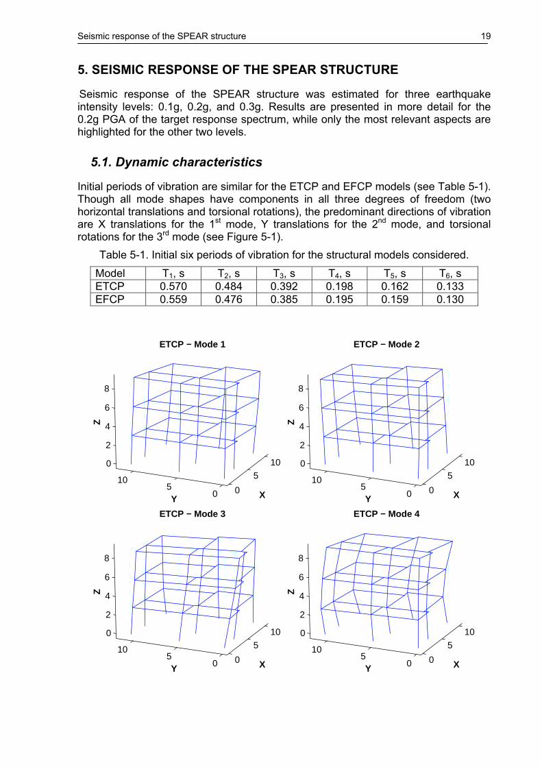
5.1. Dynamic characteristics
Initial periods of vibration are similar for the ETCP and EFCP models (see Table 5-1). Though all mode shapes have components in all three degrees of freedom (two horizontal translations and torsional rotations), the predominant directions of vibration are X translations for the 1st mode, Y translations for the 2nd mode, and torsional rotations for the 3rd mode (see Figure 5-1).
Table 5-1. Initial six periods of vibration for the structural models considered.
Model T1, s T2, s T3, s T4, s T5, s T6, s ETCP 0.570 0.484 0.392 0.198 0.162 0.133 EFCP 0.559 0.476 0.385 0.195 0.159 0.130
0
5
10
05
10
0
2
4
6
8
X
ETCP − Mode 1
Y
Z
0
5
10
05
10
0
2
4
6
8
X
ETCP − Mode 2
Y
Z
0
5
10
05
10
0
2
4
6
8
X
ETCP − Mode 3
Y
Z
0
5
10
05
10
0
2
4
6
8
X
ETCP − Mode 4
Y
Z

20 Seismic response of the SPEAR structure
0
5
10
05
10
0
2
4
6
8
X
ETCP − Mode 5
Y
Z
0
5
10
05
10
0
2
4
6
8
X
ETCP − Mode 6
Y
Z
Figure 5-1. Initial mode shapes of the ETCP model.
5.2. Earthquake intensity level 0.2g
5.2.1. Pushover analysis
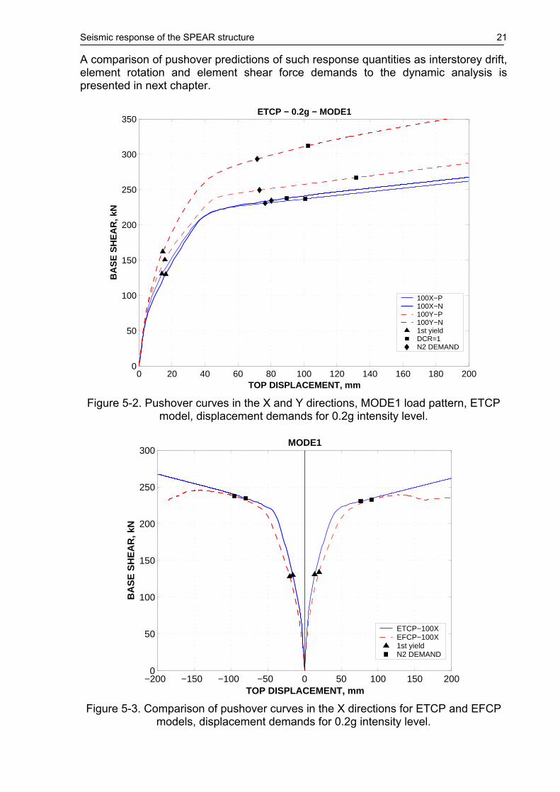
The pushover curves in the X (100X) and Y (100Y) positive (P) and negative (N) directions for the ETCP model are presented in Figure 5-2. The characteristic structural events are plotted on the graph: first element yield, displacement demand, and the attainment of ultimate rotation capacity in an element. The latter event is denoted by DCR=1, which stands for Demand to Capacity Ratio. It can be observed from the graph that base shear capacity is similar in the positive and negative X directions, but an important difference exists in the positive and negative Y directions. This behaviour is related to the strength hierarchy of elements. Generally beams negative moment capacity exceeds the column moment capacity, so that yielding occurs only in beams under positive moments and columns. However, this hierarchy is changed at the 250x750 column to beam interface, so that beams B10, B24 and B38 may experience yielding under negative moments. Thus, higher base shear capacity results for the negative Y pushover, when beams at the 250x750 column interface experience yielding in negative bending. Displacement demands were determined by the N2 method, additional details on the bilinear idealization of the capacity curve and the SDOF displacement demands being presented in ANNEX IV. Attainment of ultimate rotation capacities in elements are evaluated at displacements higher than the demands for the 0.2g earthquake intensity level. The EFCP model showed similar response as the ETCP, but the former is more flexible (see Figure 5-3 and Figure 5-4). The fibre model shows global strength degradation (initiation of failure), though at displacements much higher than the 0.2g earthquake intensity level. The degradation of strength is more pronounced in the X direction. The amount of strength degradation for the EFCP model is related to material characteristics and level of axial force in columns (represented by the pushover analysis), as well as the effects of cyclic bidirectional loading (not represented by the pushover analysis). The relative strength of steel and concrete showed to be an important parameter for column response (Stratan and Fajfar, 2002). More pronounced strength degradation of 250x250 columns was observed when characteristic material strengths were used instead of expected ones.
Seismic response of the SPEAR structure 21
A comparison of pushover predictions of such response quantities as interstorey drift, element rotation and element shear force demands to the dynamic analysis is presented in next chapter.
0 20 40 60 80 100 120 140 160 180 2000
50
100
150
200
250
300
350
TOP DISPLACEMENT, mm
BA
SE
SH
EA
R, k
NETCP − 0.2g − MODE1
100X−P100X−N100Y−P100Y−N1st yieldDCR=1N2 DEMAND
Figure 5-2. Pushover curves in the X and Y directions, MODE1 load pattern, ETCP
model, displacement demands for 0.2g intensity level.
−200 −150 −100 −50 0 50 100 150 2000
50
100
150
200
250
300
TOP DISPLACEMENT, mm
BA
SE
SH
EA
R, k
N
MODE1
ETCP−100XEFCP−100X1st yieldN2 DEMAND
Figure 5-3. Comparison of pushover curves in the X directions for ETCP and EFCP
models, displacement demands for 0.2g intensity level.
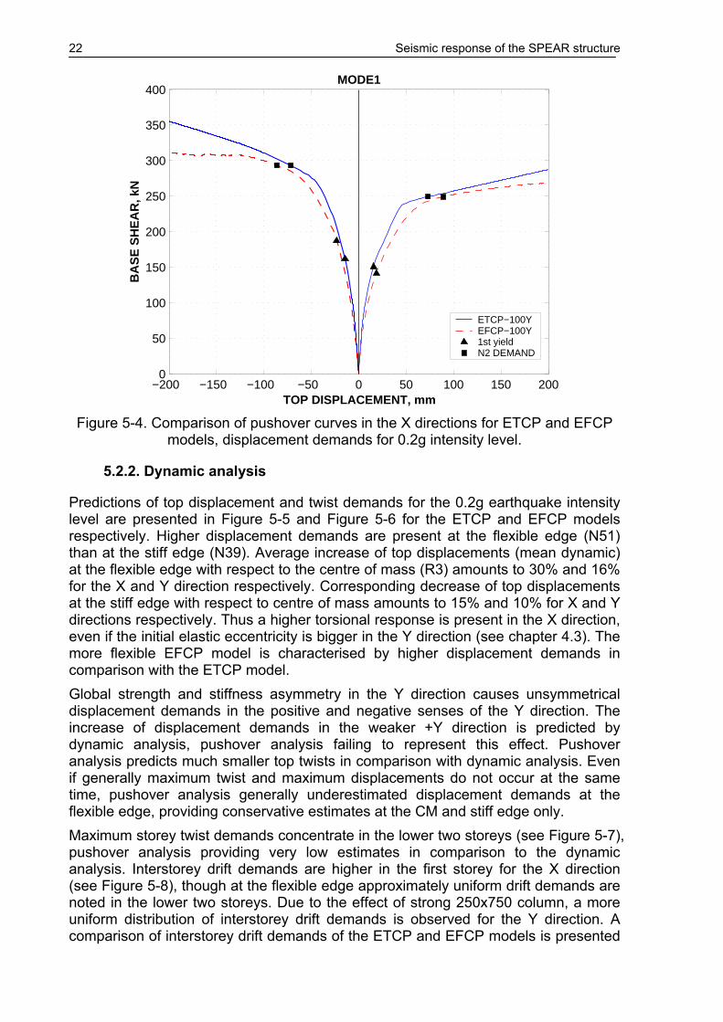
22 Seismic response of the SPEAR structure
−200 −150 −100 −50 0 50 100 150 2000
50
100
150
200
250
300
350
400
TOP DISPLACEMENT, mm
BA
SE
SH
EA
R, k
N
MODE1
ETCP−100YEFCP−100Y1st yieldN2 DEMAND
Figure 5-4. Comparison of pushover curves in the X directions for ETCP and EFCP
models, displacement demands for 0.2g intensity level.
5.2.2. Dynamic analysis
Predictions of top displacement and twist demands for the 0.2g earthquake intensity level are presented in Figure 5-5 and Figure 5-6 for the ETCP and EFCP models respectively. Higher displacement demands are present at the flexible edge (N51) than at the stiff edge (N39). Average increase of top displacements (mean dynamic) at the flexible edge with respect to the centre of mass (R3) amounts to 30% and 16% for the X and Y direction respectively. Corresponding decrease of top displacements at the stiff edge with respect to centre of mass amounts to 15% and 10% for X and Y directions respectively. Thus a higher torsional response is present in the X direction, even if the initial elastic eccentricity is bigger in the Y direction (see chapter 4.3). The more flexible EFCP model is characterised by higher displacement demands in comparison with the ETCP model. Global strength and stiffness asymmetry in the Y direction causes unsymmetrical displacement demands in the positive and negative senses of the Y direction. The increase of displacement demands in the weaker +Y direction is predicted by dynamic analysis, pushover analysis failing to represent this effect. Pushover analysis predicts much smaller top twists in comparison with dynamic analysis. Even if generally maximum twist and maximum displacements do not occur at the same time, pushover analysis generally underestimated displacement demands at the flexible edge, providing conservative estimates at the CM and stiff edge only. Maximum storey twist demands concentrate in the lower two storeys (see Figure 5-7), pushover analysis providing very low estimates in comparison to the dynamic analysis. Interstorey drift demands are higher in the first storey for the X direction (see Figure 5-8), though at the flexible edge approximately uniform drift demands are noted in the lower two storeys. Due to the effect of strong 250x750 column, a more uniform distribution of interstorey drift demands is observed for the Y direction. A comparison of interstorey drift demands of the ETCP and EFCP models is presented

Seismic response of the SPEAR structure 23
in Figure 5-10. Approximately the same distribution of drifts along the height is observed for both models, with higher demands in the case of the EFCP model.
D−RZ−R3−0.01
−0.005
0
0.005
0.01
TO
P D
ISP
LA
CE
ME
NT
, rad
ETCP − 0.2g
MEAN DYN.MEAN DYN.+STDN2−SRSS−MODE1
D−TX−R3 D−TX−N51 D−TX−N39−150
−100
−50
0
50
100
150
TO
P D
ISP
LA
CE
ME
NT
, mm
ETCP − 0.2g
MEAN DYN.MEAN DYN.+STDN2−SRSS−MODE1
D−TY−R3 D−TY−N51 D−TY−N39−150
−100
−50
0
50
100
150
TO
P D
ISP
LA
CE
ME
NT
, m
m
ETCP − 0.2g
MEAN DYN.MEAN DYN.+STDN2−SRSS−MODE1
Figure 5-5. Top twist and top displacement demands at the centre of mass (R3), stiff
(N39), and flexible (N51) edges predictions by nonlinear dynamic and pushover analyses, ETCP model, 0.2g intensity level.

24 Seismic response of the SPEAR structure
D−RZ−R3−0.015
−0.01
−0.005
0
0.005
0.01
0.015
TO
P D
ISP
LA
CE
ME
NT
, rad
EFCP − 0.2g
MEAN DYN.MEAN DYN.+STDN2−SRSS−MODE1
D−TX−R3 D−TX−N51 D−TX−N39−150
−100
−50
0
50
100
150
TO
P D
ISP
LA
CE
ME
NT
, m
m
EFCP − 0.2g
MEAN DYN.MEAN DYN.+STDN2−SRSS−MODE1
D−TY−R3 D−TY−N51 D−TY−N39−150
−100
−50
0
50
100
150
TO
P D
ISP
LA
CE
ME
NT
, mm
EFCP − 0.2g
MEAN DYN.MEAN DYN.+STDN2−SRSS−MODE1
Figure 5-6. Top twist and top displacement demands at the centre of mass (R3), stiff
(N39), and flexible (N51) edges predictions by nonlinear dynamic and pushover analyses, EFCP model, 0.2g intensity level.

Seismic response of the SPEAR structure 25
−5 0 5
x 10−3
0
2
4
6
8
10
RZ, rad
HE
IGH
T, m
ETCP − 0.2g
DYN. MEANDYN. MEAN + STDDYN. MEAN − STDN2−SRSS−MODE1
Figure 5-7. Storey twist predictions by nonlinear dynamic and pushover analyses,
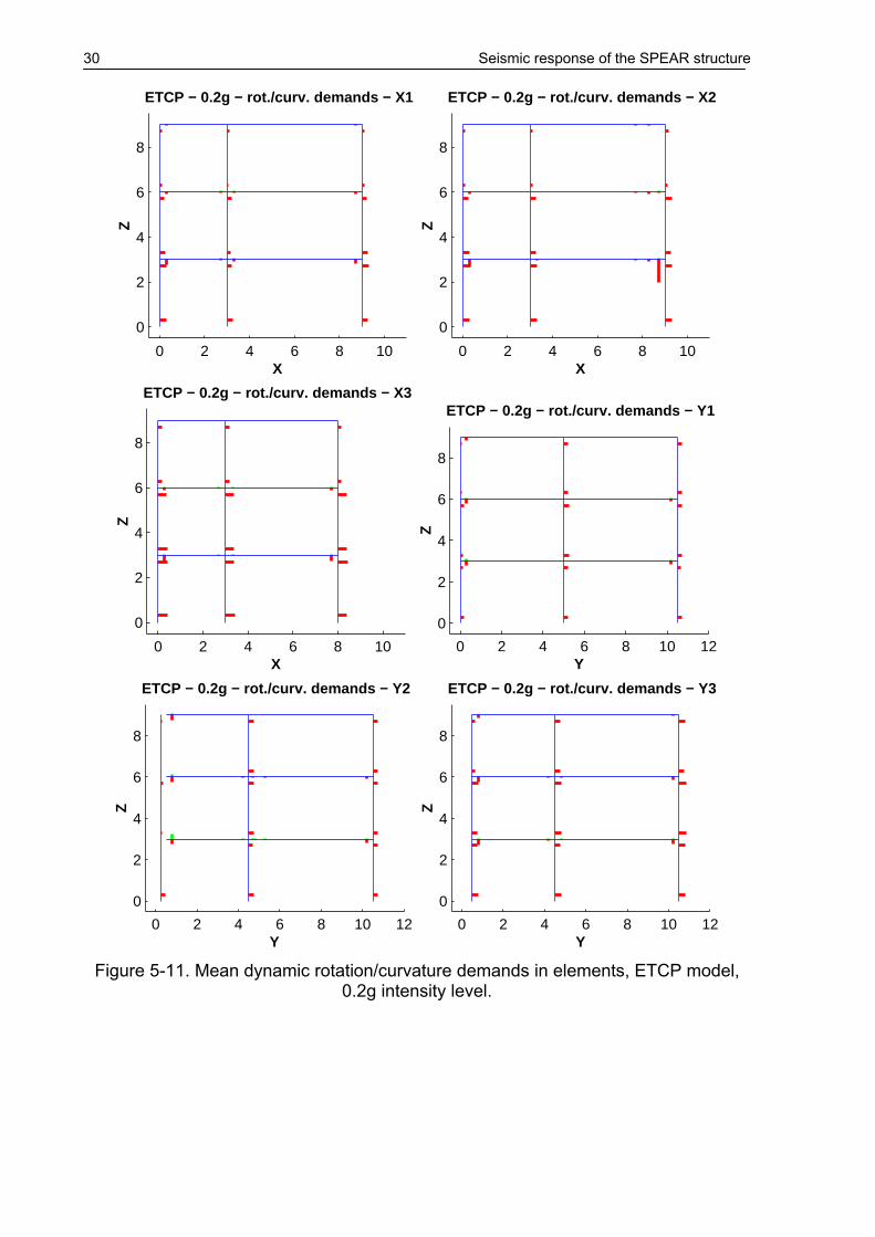
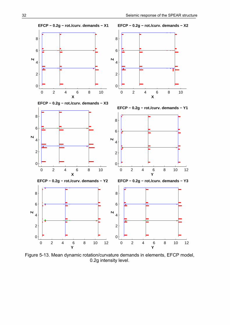
ETCP model, 0.2g intensity level. A global view of element deformation demands for the ETCP model can be observed in Figure 5-11, where either chord rotation (for most of elements) or curvature (for B13, 27, 41 and B14, 28, 42 beams) demands are plotted for the frame lines defined in Figure 4-5. In the same way, Figure 5-12 presents rotation/curvature ductility demands, only for those elements that have experienced yielding. Distinction is made in the case of beams between positive and negative bending, the latter being plotted upwards. Thus, it can be observed that the plastic mechanism is associated with extensive yielding of columns. In the X direction column ductility demands are higher in the lower two storeys, while in the Y direction they are distributed more uniformly along the height. An increase of ductility demands is present from the stiff to flexible edges (e.g. from frame line X1 towards X3). The 250x750 strong column experiences significant yielding in the Y direction at the base only, causing more uniform ductility demands in the 250x250 columns along the height of the building, and reducing the risk of a storey mechanism. Higher deformation demands are present for columns in the X direction. This is caused partially by lower top displacement demands in the Y direction, especially at the flexible edge, and especially due to more uniform drift distribution along the height (i.e. lower drift demands at the same top displacement due to a more favourable plastic mechanism). Only few beams yield under negative bending moment (top reinforcement in tension) i.e. B12i, B19j, B10i, and B24i. With the exception of the first one, these are beams framing into the strong column. Significant yielding (or pullout of bottom bars) of beams under positive bending moments is however present, mainly for shorter beams and/or at the exterior beam-column joints, where there is greater chance of moment reversal due to earthquake loading. The same conclusions can be observed from the chord rotation and curvature demands pots in the case of the EFCP model (Figure 5-13). Note that in this case curvatures are plotted for columns modelled by fibre elements.
26 Seismic response of the SPEAR structure
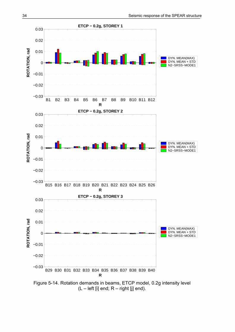
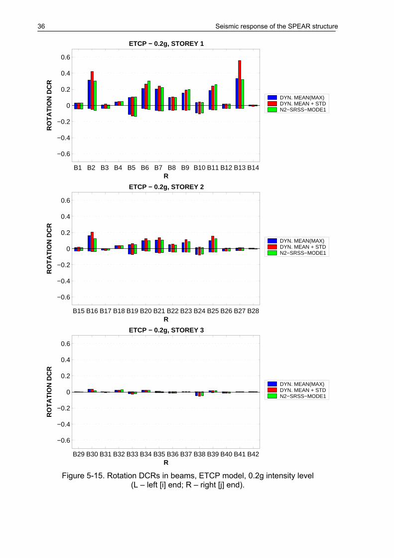
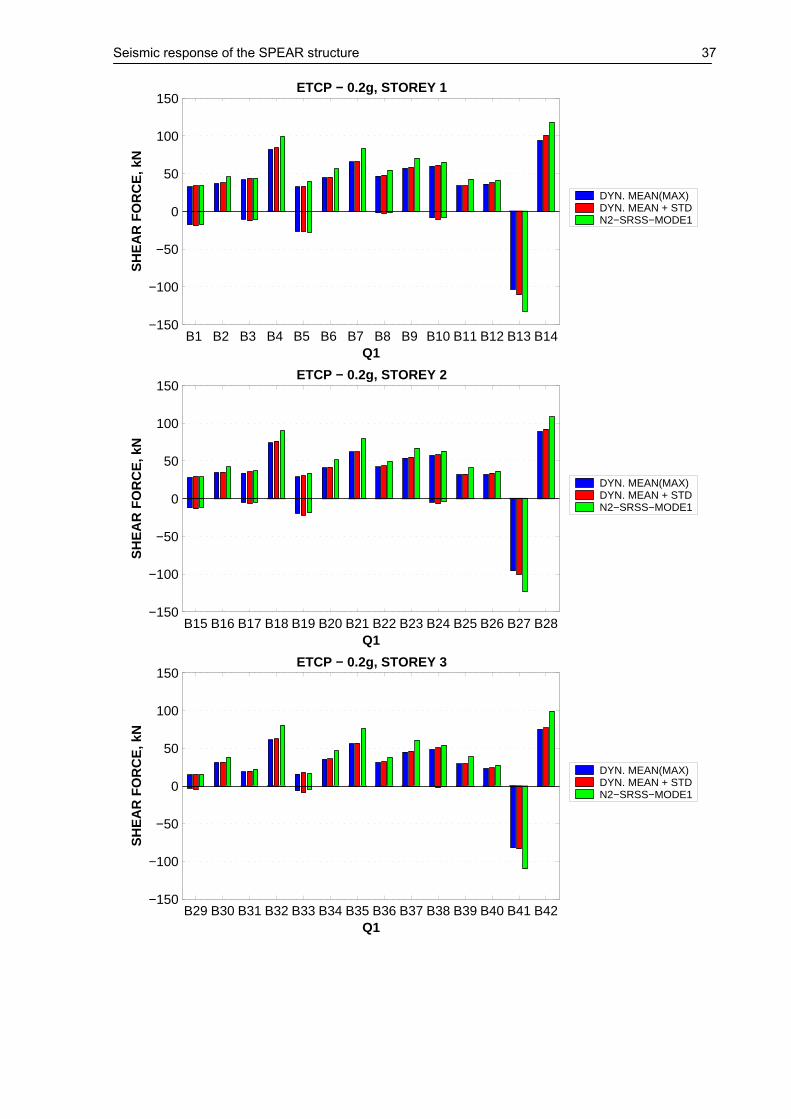
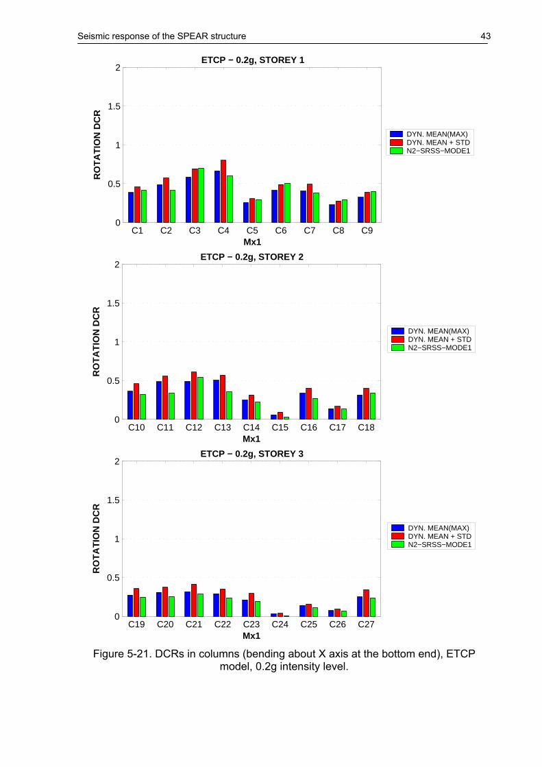
Mean dynamic and pushover estimates of beams chord rotations for the ETCP model are presented in Figure 5-14. A reasonable agreement between the two analysis methods is noted. At the same time, the relatively reduced values of rotations in beams are noted, especially when compared to the capacity. The Demand to Capacity Ratios (DCRs) in terms of rotations or curvatures are plotted in Figure 5-15. All of the beams have DCRs less than unity. Diagrams of elastic shear force demands (Figure 5-16) show that with the exception of short beams B1, B3, B5 and the corresponding upper storey ones, no or little shear force reversal occurs. Plots of rotation demands in columns (Figure 5-17 through Figure 5-20) show trends in accordance with drift distributions. Thus, in the case of bending about the global Y axis (corresponding to X direction displacement demands), column rotation demands are higher in the lower two stories. For bending about the X axis, rotations are more uniform across the three stories. Due to concentration of deformations in the lower two stories in the X direction, rotation demands in the corresponding columns are considerably higher for bending about the Y axis than for bending about the X axis. Columns at the flexible edges experience higher rotation demands than the ones at the stiff edges. Column rotation DCRs are presented in Figure 5-21 through Figure 5-24. The maximum DCRs are observed for columns with high rotation demands (at the flexible edges) and low rotation capacities (higher axially loaded first storey columns). For bending about the X axis, the critical columns are C2, C3, and C4. The same ones, in addition to C1 represent the critical elements for bending about the Y axis. However, the highest DCR of 0.81 for the C3 column shows that the SPEAR structure will resist the 0.2g intensity earthquake without collapse. Shear force demands in columns for the ETCP model are presented in Figure 5-25 and Figure 5-26. In the case of EFCP model somewhat higher rotation demands (see Figure 5-27) and similar shear force demands (see Figure 5-28) in beams were observed. Column flexural response is not comparable directly due to different element formulation, however, the shear force demands were similar for the two models (Figure 5-29). Significant concrete compressive strains in the softening range were observed for C1 to C4 columns, in agreement with the ETCP model. Concrete spalling is expected for these elements. Sample moment-rotation and moment-curvature response of the beam B1, and columns C2 and C3 for the ETCP and EFCP models are presented in Figure 5-30 through Figure 5-35. Only one or few full cycles in the inelastic range are generally observed. Though generally column response was characterised by stable hysteresis loops in the case of EFCP model, in several cases (e.g. C2 column under AL2-0 record) considerable strength degradation was observed, indicating element failure. Time histories of top displacements and twists for both models are presented in Figure 5-36 through Figure 5-39. Top displacements at the flexible and stiff edges are generally in phase, especially for the pre-peak range. Contrary, top twist is generally not in phase with displacements. Investigation of unidirectional vs. bidirectional seismic input in a companion study (Stratan and Fajfar, 2002) showed that under unidirectional seismic input both top displacements and twist were in phase. Top twist time history is affected significantly by the bidirectional seismic input, maximum values being always higher than the ones under unidirectional input. Contrary, top displacements in a given direction under bidirectional seismic input are governed by the unidirectional time history response in the same direction, and can both increase or decrease in magnitude with respect to the unidirectional input.

Seismic response of the SPEAR structure 27
However, as the influence of the seismic input in the orthogonal direction on top translations is comparatively small, the displacements at the stiff and flexible edges are generally in phase also under bidirectional seismic input, at least for highest peaks.
−0.015−0.01−0.005 0 0.005 0.010
2
4
6
8
10
TX, rad
HE
IGH
T, m
ETCP − 0.2g
DYN. MEANDYN. MEAN + STDDYN. MEAN − STDN2−SRSS−MODE1
−0.015−0.01−0.005 0 0.005 0.010
2
4
6
8
10
TX, rad
HE
IGH
T, m
ETCP − 0.2g − X1Y1
DYN. MEANDYN. MEAN + STDDYN. MEAN − STDN2−SRSS−MODE1
−0.02 −0.01 0 0.01 0.020
2
4
6
8
10
TX, rad
HE
IGH
T, m
ETCP − 0.2g − X3Y3
DYN. MEANDYN. MEAN + STDDYN. MEAN − STDN2−SRSS−MODE1
Figure 5-8. Interstorey displacement demands in the X direction at the centre of mass
(CM), stiff (X1Y1), and flexible (X3Y3) edges, ETCP model, 0.2g intensity level.

28 Seismic response of the SPEAR structure
−0.015−0.01−0.005 0 0.005 0.010
2
4
6
8
10
TY, rad
HE
IGH
T, m
ETCP − 0.2g
DYN. MEANDYN. MEAN + STDDYN. MEAN − STDN2−SRSS−MODE1
−0.015−0.01−0.005 0 0.005 0.010
2
4
6
8
10
TY, rad
HE
IGH
T, m
ETCP − 0.2g − X1Y1
DYN. MEANDYN. MEAN + STDDYN. MEAN − STDN2−SRSS−MODE1
−0.015−0.01−0.005 0 0.005 0.010
2
4
6
8
10
TY, rad
HE
IGH
T, m
ETCP − 0.2g − X3Y3
DYN. MEANDYN. MEAN + STDDYN. MEAN − STDN2−SRSS−MODE1
Figure 5-9. Interstorey displacement demands in the Y direction at the centre of mass
(CM), stiff (X1Y1), and flexible (X3Y3) edges, ETCP model, 0.2g intensity level.

Seismic response of the SPEAR structure 29
−0.015−0.01−0.005 0 0.005 0.010
2
4
6
8
10
TX, rad
HE
IGH
T, m
MEAN DYNAMIC − 0.2g − CM
ETCPEFCP
−0.015−0.01−0.005 0 0.005 0.010
2
4
6
8
10
TY, rad
HE
IGH
T, m
MEAN DYNAMIC − 0.2g − CM
ETCPEFCP
−0.015−0.01−0.005 0 0.005 0.010
2
4
6
8
10
TX, rad
HE
IGH
T, m
MEAN DYNAMIC − 0.2g − X1Y1
ETCPEFCP
−0.015−0.01−0.005 0 0.005 0.010
2
4
6
8
10
TY, rad
HE
IGH
T, m
MEAN DYNAMIC − 0.2g − X1Y1
ETCPEFCP
−0.02 −0.01 0 0.01 0.020
2
4
6
8
10
TX, rad
HE
IGH
T, m
MEAN DYNAMIC − 0.2g − X3Y3
ETCPEFCP
−0.015−0.01−0.005 0 0.005 0.010
2
4
6
8
10
TY, rad
HE
IGH
T, m
MEAN DYNAMIC − 0.2g − X3Y3
ETCPEFCP
Figure 5-10. Comparison of interstorey drift demands for the ETCP and EFCP
models at the centre of mass (CM), stiff (X1Y1), and flexible (X3Y3) edges.
30 Seismic response of the SPEAR structure
0 2 4 6 8 10
0
2
4
6
8
ETCP − 0.2g − rot./curv. demands − X1
X
Z
0 2 4 6 8 10
0
2
4
6
8
ETCP − 0.2g − rot./curv. demands − X2
X
Z
0 2 4 6 8 10
0
2
4
6
8
ETCP − 0.2g − rot./curv. demands − X3
X
Z
0 2 4 6 8 10 12
0
2
4
6
8
ETCP − 0.2g − rot./curv. demands − Y1
Y
Z
0 2 4 6 8 10 12
0
2
4
6
8
ETCP − 0.2g − rot./curv. demands − Y2
Y
Z
0 2 4 6 8 10 12
0
2
4
6
8
ETCP − 0.2g − rot./curv. demands − Y3
Y
Z
Figure 5-11. Mean dynamic rotation/curvature demands in elements, ETCP model,
0.2g intensity level.

Seismic response of the SPEAR structure 31
0 2 4 6 8 10
0
2
4
6
8
ETCP − 0.2g − ductility demands − X1
X
Z
0 2 4 6 8 10
0
2
4
6
8
ETCP − 0.2g − ductility demands − X2
X
Z
0 2 4 6 8 10
0
2
4
6
8
ETCP − 0.2g − ductility demands − X3
X
Z
0 2 4 6 8 10 12
0
2
4
6
8
ETCP − 0.2g − ductility demands − Y1
Y
Z
0 2 4 6 8 10 12
0
2
4
6
8
ETCP − 0.2g − ductility demands − Y2
Y
Z
0 2 4 6 8 10 12
0
2
4
6
8
ETCP − 0.2g − ductility demands − Y3
Y
Z
Figure 5-12. Mean dynamic rotation/curvature ductility demands in elements, ETCP
model, 0.2g intensity level.
32 Seismic response of the SPEAR structure
0 2 4 6 8 10
0
2
4
6
8
EFCP − 0.2g − rot./curv. demands − X1
X
Z
0 2 4 6 8 10
0
2
4
6
8
EFCP − 0.2g − rot./curv. demands − X2
X
Z
0 2 4 6 8 10
0
2
4
6
8
EFCP − 0.2g − rot./curv. demands − X3
X
Z
0 2 4 6 8 10 12
0
2
4
6
8
EFCP − 0.2g − rot./curv. demands − Y1
Y
Z
0 2 4 6 8 10 12
0
2
4
6
8
EFCP − 0.2g − rot./curv. demands − Y2
Y
Z
0 2 4 6 8 10 12
0
2
4
6
8
EFCP − 0.2g − rot./curv. demands − Y3
Y
Z
Figure 5-13. Mean dynamic rotation/curvature demands in elements, EFCP model,
0.2g intensity level.

Seismic response of the SPEAR structure 33
B1 B2 B3 B4 B5 B6 B7 B8 B9 B10 B11 B12−0.03
−0.02
−0.01
0
0.01
0.02
0.03
L
RO
TA
TIO
N, r
ad
ETCP − 0.2g, STOREY 1
DYN. MEAN(MAX)DYN. MEAN + STDN2−SRSS−MODE1
B15 B16 B17 B18 B19 B20 B21 B22 B23 B24 B25 B26−0.03
−0.02
−0.01
0
0.01
0.02
0.03
L
RO
TA
TIO
N, r
ad
ETCP − 0.2g, STOREY 2
DYN. MEAN(MAX)DYN. MEAN + STDN2−SRSS−MODE1
B29 B30 B31 B32 B33 B34 B35 B36 B37 B38 B39 B40−0.03
−0.02
−0.01
0
0.01
0.02
0.03
L
RO
TA
TIO
N, r
ad
ETCP − 0.2g, STOREY 3
DYN. MEAN(MAX)DYN. MEAN + STDN2−SRSS−MODE1
34 Seismic response of the SPEAR structure
B1 B2 B3 B4 B5 B6 B7 B8 B9 B10 B11 B12−0.03
−0.02
−0.01
0
0.01
0.02
0.03
R
RO
TA
TIO
N, r
adETCP − 0.2g, STOREY 1
DYN. MEAN(MAX)DYN. MEAN + STDN2−SRSS−MODE1
B15 B16 B17 B18 B19 B20 B21 B22 B23 B24 B25 B26−0.03
−0.02
−0.01
0
0.01
0.02
0.03
R
RO
TA
TIO
N, r
ad
ETCP − 0.2g, STOREY 2
DYN. MEAN(MAX)DYN. MEAN + STDN2−SRSS−MODE1
B29 B30 B31 B32 B33 B34 B35 B36 B37 B38 B39 B40−0.03
−0.02
−0.01
0
0.01
0.02
0.03
R
RO
TA
TIO
N, r
ad
ETCP − 0.2g, STOREY 3
DYN. MEAN(MAX)DYN. MEAN + STDN2−SRSS−MODE1
Figure 5-14. Rotation demands in beams, ETCP model, 0.2g intensity level
(L – left [i] end; R – right [j] end).

Seismic response of the SPEAR structure 35
B1 B2 B3 B4 B5 B6 B7 B8 B9 B10 B11 B12 B13 B14
−0.6
−0.4
−0.2
0
0.2
0.4
0.6
L
RO
TA
TIO
N D
CR
ETCP − 0.2g, STOREY 1
DYN. MEAN(MAX)DYN. MEAN + STDN2−SRSS−MODE1
B15 B16 B17 B18 B19 B20 B21 B22 B23 B24 B25 B26 B27 B28
−0.6
−0.4
−0.2
0
0.2
0.4
0.6
L
RO
TA
TIO
N D
CR
ETCP − 0.2g, STOREY 2
DYN. MEAN(MAX)DYN. MEAN + STDN2−SRSS−MODE1
B29 B30 B31 B32 B33 B34 B35 B36 B37 B38 B39 B40 B41 B42
−0.6
−0.4
−0.2
0
0.2
0.4
0.6
L
RO
TA
TIO
N D
CR
ETCP − 0.2g, STOREY 3
DYN. MEAN(MAX)DYN. MEAN + STDN2−SRSS−MODE1
36 Seismic response of the SPEAR structure
B1 B2 B3 B4 B5 B6 B7 B8 B9 B10 B11 B12 B13 B14
−0.6
−0.4
−0.2
0
0.2
0.4
0.6
R
RO
TA
TIO
N D
CR
ETCP − 0.2g, STOREY 1
DYN. MEAN(MAX)DYN. MEAN + STDN2−SRSS−MODE1
B15 B16 B17 B18 B19 B20 B21 B22 B23 B24 B25 B26 B27 B28
−0.6
−0.4
−0.2
0
0.2
0.4
0.6
R
RO
TA
TIO
N D
CR
ETCP − 0.2g, STOREY 2
DYN. MEAN(MAX)DYN. MEAN + STDN2−SRSS−MODE1
B29 B30 B31 B32 B33 B34 B35 B36 B37 B38 B39 B40 B41 B42
−0.6
−0.4
−0.2
0
0.2
0.4
0.6
R
RO
TA
TIO
N D
CR
ETCP − 0.2g, STOREY 3
DYN. MEAN(MAX)DYN. MEAN + STDN2−SRSS−MODE1
Figure 5-15. Rotation DCRs in beams, ETCP model, 0.2g intensity level
(L – left [i] end; R – right [j] end).
Seismic response of the SPEAR structure 37
B1 B2 B3 B4 B5 B6 B7 B8 B9 B10 B11 B12 B13 B14−150
−100
−50
0
50
100
150
Q1
SH
EA
R F
OR
CE
, kN
ETCP − 0.2g, STOREY 1
DYN. MEAN(MAX)DYN. MEAN + STDN2−SRSS−MODE1
B15 B16 B17 B18 B19 B20 B21 B22 B23 B24 B25 B26 B27 B28−150
−100
−50
0
50
100
150
Q1
SH
EA
R F
OR
CE
, kN
ETCP − 0.2g, STOREY 2
DYN. MEAN(MAX)DYN. MEAN + STDN2−SRSS−MODE1
B29 B30 B31 B32 B33 B34 B35 B36 B37 B38 B39 B40 B41 B42−150
−100
−50
0
50
100
150
Q1
SH
EA
R F
OR
CE
, kN
ETCP − 0.2g, STOREY 3
DYN. MEAN(MAX)DYN. MEAN + STDN2−SRSS−MODE1

38 Seismic response of the SPEAR structure
B1 B2 B3 B4 B5 B6 B7 B8 B9 B10 B11 B12 B13 B14−150
−100
−50
0
50
100
150
Q2
SH
EA
R F
OR
CE
, kN
ETCP − 0.2g, STOREY 1
DYN. MEAN(MAX)DYN. MEAN + STDN2−SRSS−MODE1
B15 B16 B17 B18 B19 B20 B21 B22 B23 B24 B25 B26 B27 B28−150
−100
−50
0
50
100
150
Q2
SH
EA
R F
OR
CE
, kN
ETCP − 0.2g, STOREY 2
DYN. MEAN(MAX)DYN. MEAN + STDN2−SRSS−MODE1
B29 B30 B31 B32 B33 B34 B35 B36 B37 B38 B39 B40 B41 B42−150
−100
−50
0
50
100
150
Q2
SH
EA
R F
OR
CE
, kN
ETCP − 0.2g, STOREY 3
DYN. MEAN(MAX)DYN. MEAN + STDN2−SRSS−MODE1
Figure 5-16. Shear force demands in beams, ETCP model, 0.2g intensity level
(Q1 – end I, Q2 – end j).

Seismic response of the SPEAR structure 39
C1 C2 C3 C4 C5 C6 C7 C8 C90
0.005
0.01
0.015
0.02
0.025
0.03
0.035
Mx1
RO
TA
TIO
N, r
ad
ETCP − 0.2g, STOREY 1
DYN. MEAN(MAX)DYN. MEAN + STDN2−SRSS−MODE1
C10 C11 C12 C13 C14 C15 C16 C17 C180
0.005
0.01
0.015
0.02
0.025
0.03
0.035
Mx1
RO
TA
TIO
N, r
ad
ETCP − 0.2g, STOREY 2
DYN. MEAN(MAX)DYN. MEAN + STDN2−SRSS−MODE1
C19 C20 C21 C22 C23 C24 C25 C26 C270
0.005
0.01
0.015
0.02
0.025
0.03
0.035
Mx1
RO
TA
TIO
N, r
ad
ETCP − 0.2g, STOREY 3
DYN. MEAN(MAX)DYN. MEAN + STDN2−SRSS−MODE1
Figure 5-17. Rotation demands in columns (bending about X axis at the bottom end),
ETCP model, 0.2g intensity level.

40 Seismic response of the SPEAR structure
C1 C2 C3 C4 C5 C6 C7 C8 C90
0.005
0.01
0.015
0.02
0.025
0.03
0.035
My1
RO
TA
TIO
N, r
adETCP − 0.2g, STOREY 1
DYN. MEAN(MAX)DYN. MEAN + STDN2−SRSS−MODE1
C10 C11 C12 C13 C14 C15 C16 C17 C180
0.005
0.01
0.015
0.02
0.025
0.03
0.035
My1
RO
TA
TIO
N, r
ad
ETCP − 0.2g, STOREY 2
DYN. MEAN(MAX)DYN. MEAN + STDN2−SRSS−MODE1
C19 C20 C21 C22 C23 C24 C25 C26 C270
0.005
0.01
0.015
0.02
0.025
0.03
0.035
My1
RO
TA
TIO
N, r
ad
ETCP − 0.2g, STOREY 3
DYN. MEAN(MAX)DYN. MEAN + STDN2−SRSS−MODE1
Figure 5-18. Rotation demands in columns (bending about Y axis at the bottom end),
ETCP model, 0.2g intensity level.

Seismic response of the SPEAR structure 41
C1 C2 C3 C4 C5 C6 C7 C8 C90
0.005
0.01
0.015
0.02
0.025
0.03
0.035
Mx2
RO
TA
TIO
N, r
ad
ETCP − 0.2g, STOREY 1
DYN. MEAN(MAX)DYN. MEAN + STDN2−SRSS−MODE1
C10 C11 C12 C13 C14 C15 C16 C17 C180
0.005
0.01
0.015
0.02
0.025
0.03
0.035
Mx2
RO
TA
TIO
N, r
ad
ETCP − 0.2g, STOREY 2
DYN. MEAN(MAX)DYN. MEAN + STDN2−SRSS−MODE1
C19 C20 C21 C22 C23 C24 C25 C26 C270
0.005
0.01
0.015
0.02
0.025
0.03
0.035
Mx2
RO
TA
TIO
N, r
ad
ETCP − 0.2g, STOREY 3
DYN. MEAN(MAX)DYN. MEAN + STDN2−SRSS−MODE1
Figure 5-19. Rotation demands in columns (bending about X axis at the top end),
ETCP model, 0.2g intensity level.

42 Seismic response of the SPEAR structure
C1 C2 C3 C4 C5 C6 C7 C8 C90
0.005
0.01
0.015
0.02
0.025
0.03
0.035
My2
RO
TA
TIO
N, r
adETCP − 0.2g, STOREY 1
DYN. MEAN(MAX)DYN. MEAN + STDN2−SRSS−MODE1
C10 C11 C12 C13 C14 C15 C16 C17 C180
0.005
0.01
0.015
0.02
0.025
0.03
0.035
My2
RO
TA
TIO
N, r
ad
ETCP − 0.2g, STOREY 2
DYN. MEAN(MAX)DYN. MEAN + STDN2−SRSS−MODE1
C19 C20 C21 C22 C23 C24 C25 C26 C270
0.005
0.01
0.015
0.02
0.025
0.03
0.035
My2
RO
TA
TIO
N, r
ad
ETCP − 0.2g, STOREY 3
DYN. MEAN(MAX)DYN. MEAN + STDN2−SRSS−MODE1
Figure 5-20. Rotation demands in columns (bending about Y axis at the top end),
ETCP model, 0.2g intensity level.
Seismic response of the SPEAR structure 43
C1 C2 C3 C4 C5 C6 C7 C8 C90
0.5
1
1.5
2
Mx1
RO
TA
TIO
N D
CR
ETCP − 0.2g, STOREY 1
DYN. MEAN(MAX)DYN. MEAN + STDN2−SRSS−MODE1
C10 C11 C12 C13 C14 C15 C16 C17 C180
0.5
1
1.5
2
Mx1
RO
TA
TIO
N D
CR
ETCP − 0.2g, STOREY 2
DYN. MEAN(MAX)DYN. MEAN + STDN2−SRSS−MODE1
C19 C20 C21 C22 C23 C24 C25 C26 C270
0.5
1
1.5
2
Mx1
RO
TA
TIO
N D
CR
ETCP − 0.2g, STOREY 3
DYN. MEAN(MAX)DYN. MEAN + STDN2−SRSS−MODE1
Figure 5-21. DCRs in columns (bending about X axis at the bottom end), ETCP
model, 0.2g intensity level.

44 Seismic response of the SPEAR structure
C1 C2 C3 C4 C5 C6 C7 C8 C90
0.5
1
1.5
2
My1
RO
TA
TIO
N D
CR
ETCP − 0.2g, STOREY 1
DYN. MEAN(MAX)DYN. MEAN + STDN2−SRSS−MODE1
C10 C11 C12 C13 C14 C15 C16 C17 C180
0.5
1
1.5
2
My1
RO
TA
TIO
N D
CR
ETCP − 0.2g, STOREY 2
DYN. MEAN(MAX)DYN. MEAN + STDN2−SRSS−MODE1
C19 C20 C21 C22 C23 C24 C25 C26 C270
0.5
1
1.5
2
My1
RO
TA
TIO
N D
CR
ETCP − 0.2g, STOREY 3
DYN. MEAN(MAX)DYN. MEAN + STDN2−SRSS−MODE1
Figure 5-22. DCRs in columns (bending about Y axis at the bottom end), ETCP
model, 0.2g intensity level.
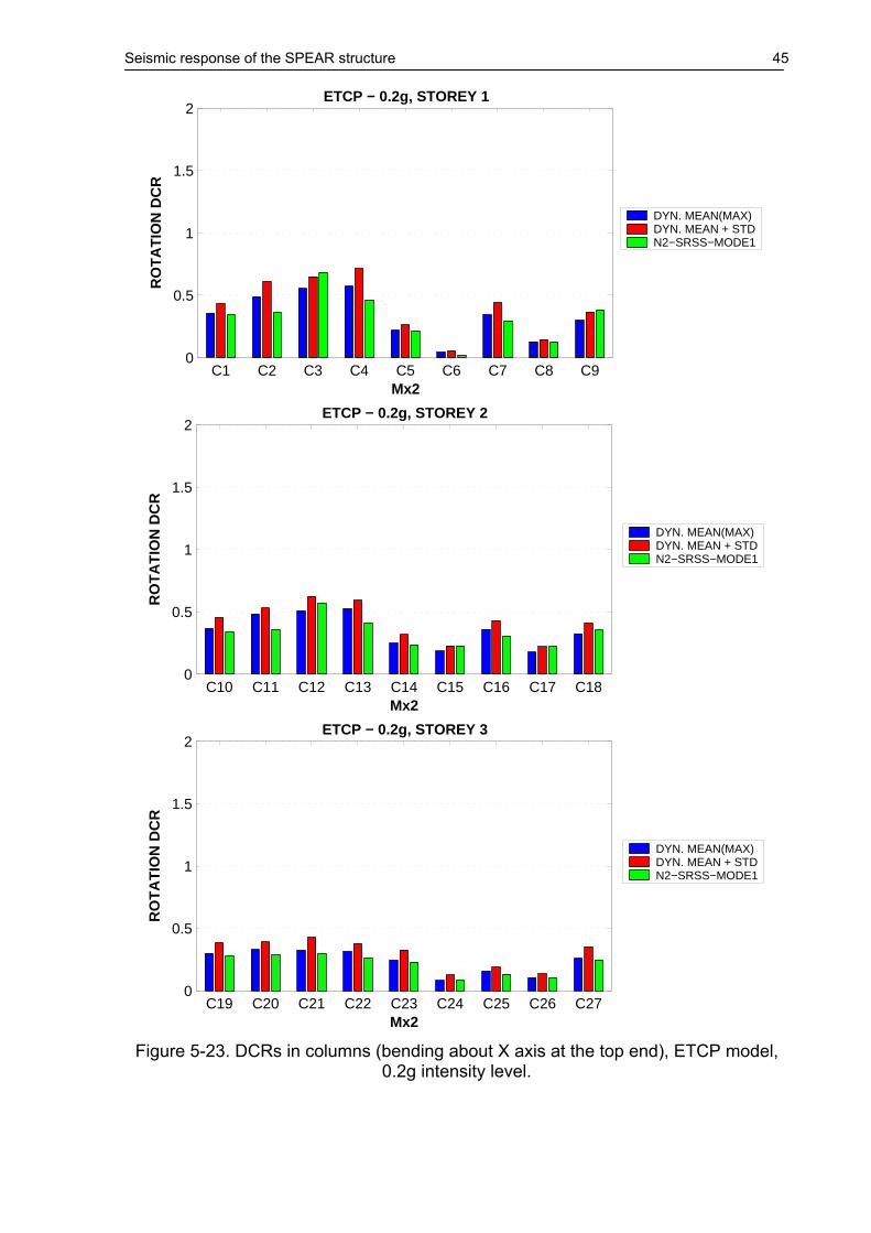
Seismic response of the SPEAR structure 45
C1 C2 C3 C4 C5 C6 C7 C8 C90
0.5
1
1.5
2
Mx2
RO
TA
TIO
N D
CR
ETCP − 0.2g, STOREY 1
DYN. MEAN(MAX)DYN. MEAN + STDN2−SRSS−MODE1
C10 C11 C12 C13 C14 C15 C16 C17 C180
0.5
1
1.5
2
Mx2
RO
TA
TIO
N D
CR
ETCP − 0.2g, STOREY 2
DYN. MEAN(MAX)DYN. MEAN + STDN2−SRSS−MODE1
C19 C20 C21 C22 C23 C24 C25 C26 C270
0.5
1
1.5
2
Mx2
RO
TA
TIO
N D
CR
ETCP − 0.2g, STOREY 3
DYN. MEAN(MAX)DYN. MEAN + STDN2−SRSS−MODE1
Figure 5-23. DCRs in columns (bending about X axis at the top end), ETCP model,
0.2g intensity level.

46 Seismic response of the SPEAR structure
C1 C2 C3 C4 C5 C6 C7 C8 C90
0.5
1
1.5
2
My2
RO
TA
TIO
N D
CR
ETCP − 0.2g, STOREY 1
DYN. MEAN(MAX)DYN. MEAN + STDN2−SRSS−MODE1
C10 C11 C12 C13 C14 C15 C16 C17 C180
0.5
1
1.5
2
My2
RO
TA
TIO
N D
CR
ETCP − 0.2g, STOREY 2
DYN. MEAN(MAX)DYN. MEAN + STDN2−SRSS−MODE1
C19 C20 C21 C22 C23 C24 C25 C26 C270
0.5
1
1.5
2
My2
RO
TA
TIO
N D
CR
ETCP − 0.2g, STOREY 3
DYN. MEAN(MAX)DYN. MEAN + STDN2−SRSS−MODE1
Figure 5-24. DCRs in columns (bending about Y axis at the top end), ETCP model,
0.2g intensity level.

Seismic response of the SPEAR structure 47
C1 C2 C3 C4 C5 C6 C7 C8 C90
20
40
60
80
100
120
140
Sx
SH
EA
R F
OR
CE
, kN
ETCP − 0.2g, STOREY 1
DYN. MEAN(MAX)DYN. MEAN + STDN2−SRSS−MODE1
C10 C11 C12 C13 C14 C15 C16 C17 C180
20
40
60
80
100
120
140
Sx
SH
EA
R F
OR
CE
, kN
ETCP − 0.2g, STOREY 2
DYN. MEAN(MAX)DYN. MEAN + STDN2−SRSS−MODE1
C19 C20 C21 C22 C23 C24 C25 C26 C270
20
40
60
80
100
120
140
Sx
SH
EA
R F
OR
CE
, kN
ETCP − 0.2g, STOREY 3
DYN. MEAN(MAX)DYN. MEAN + STDN2−SRSS−MODE1
Figure 5-25. Shear force demands in columns (along X axis), ETCP model, 0.2g
intensity level.

48 Seismic response of the SPEAR structure
C1 C2 C3 C4 C5 C6 C7 C8 C90
20
40
60
80
100
120
140
Sy
SH
EA
R F
OR
CE
, kN
ETCP − 0.2g, STOREY 1
DYN. MEAN(MAX)DYN. MEAN + STDN2−SRSS−MODE1
C10 C11 C12 C13 C14 C15 C16 C17 C180
20
40
60
80
100
120
140
Sy
SH
EA
R F
OR
CE
, kN
ETCP − 0.2g, STOREY 2
DYN. MEAN(MAX)DYN. MEAN + STDN2−SRSS−MODE1
C19 C20 C21 C22 C23 C24 C25 C26 C270
20
40
60
80
100
120
140
Sy
SH
EA
R F
OR
CE
, kN
ETCP − 0.2g, STOREY 3
DYN. MEAN(MAX)DYN. MEAN + STDN2−SRSS−MODE1
Figure 5-26. Shear force demands in columns (along Y axis), ETCP model, 0.2g
intensity level.

Seismic response of the SPEAR structure 49
B1 B2 B3 B4 B5 B6 B7 B8 B9 B10 B11 B12−0.03
−0.02
−0.01
0
0.01
0.02
0.03
L
RO
TA
TIO
N, r
ad
0.2g − STOREY 1
ETCPEFCP
Figure 5-27. Rotation demands in storey 1 beams left end, ETCP vs. EFCP models,
0.2g intensity level.
B1 B2 B3 B4 B5 B6 B7 B8 B9 B10 B11 B12 B13 B14−150
−100
−50
0
50
100
150
Q1
SH
EA
R F
OR
CE
, kN
0.2g − STOREY 1
ETCPEFCP
Figure 5-28. Shear force demands in storey 1 beams left end, ETCP vs. EFCP
models, 0.2g intensity level.

50 Seismic response of the SPEAR structure
C1 C2 C3 C4 C5 C6 C7 C8 C90
20
40
60
80
100
120
140
Sx
SH
EA
R F
OR
CE
, kN
0.2g − STOREY 1
ETCPEFCP
C1 C2 C3 C4 C5 C6 C7 C8 C90
20
40
60
80
100
120
140
Sy
SH
EA
R F
OR
CE
, kN
0.2g − STOREY 1
ETCPEFCP
Figure 5-29. Shear force demands in storey 1 columns (along X and Y axes), ETCP
vs. EFCP models, 0.2g intensity level.
−0.02 −0.01 0 0.01 0.02−60
−40
−20
0
20
40
60
L − ROTATION, rad
MO
ME
NT
, kN
m
ETCP − 0.2g − B1 − AL1−0
−0.02 −0.01 0 0.01 0.02−60
−40
−20
0
20
40
60
L − ROTATION, rad
MO
ME
NT
, kN
m
ETCP − 0.2g − B1 − AL2−0
Figure 5-30. Moment-rotation history for the beam B1 left end (i), ETCP model, AL1-0
and AL2-0 records, 0.2g intensity level.
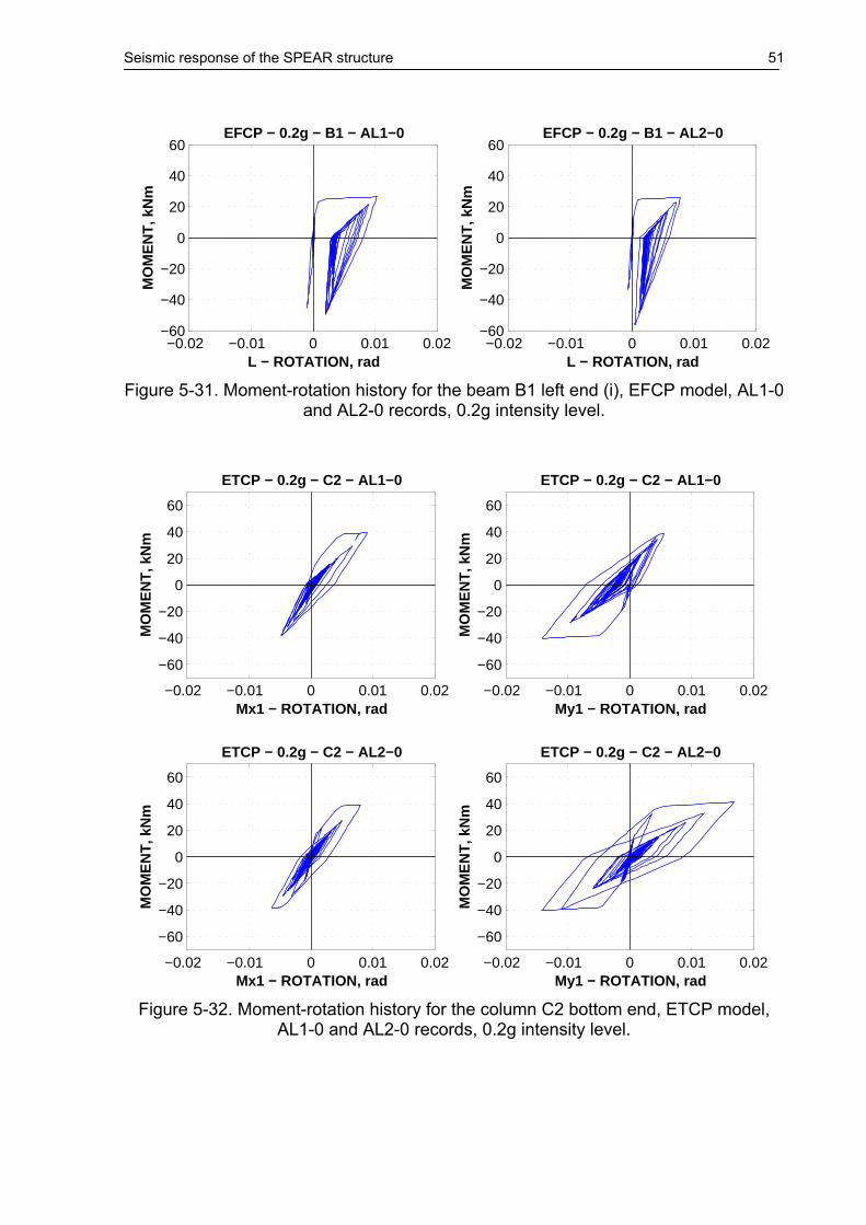
Seismic response of the SPEAR structure 51
−0.02 −0.01 0 0.01 0.02−60
−40
−20
0
20
40
60
L − ROTATION, rad
MO
ME
NT
, kN
mEFCP − 0.2g − B1 − AL1−0
−0.02 −0.01 0 0.01 0.02−60
−40
−20
0
20
40
60
L − ROTATION, rad
MO
ME
NT
, kN
m
EFCP − 0.2g − B1 − AL2−0
Figure 5-31. Moment-rotation history for the beam B1 left end (i), EFCP model, AL1-0
and AL2-0 records, 0.2g intensity level.
−0.02 −0.01 0 0.01 0.02
−60
−40
−20
0
20
40
60
Mx1 − ROTATION, rad
MO
ME
NT
, kN
m
ETCP − 0.2g − C2 − AL1−0
−0.02 −0.01 0 0.01 0.02
−60
−40
−20
0
20
40
60
My1 − ROTATION, rad
MO
ME
NT
, kN
mETCP − 0.2g − C2 − AL1−0
−0.02 −0.01 0 0.01 0.02
−60
−40
−20
0
20
40
60
Mx1 − ROTATION, rad
MO
ME
NT
, kN
m
ETCP − 0.2g − C2 − AL2−0
−0.02 −0.01 0 0.01 0.02
−60
−40
−20
0
20
40
60
My1 − ROTATION, rad
MO
ME
NT
, kN
m
ETCP − 0.2g − C2 − AL2−0
Figure 5-32. Moment-rotation history for the column C2 bottom end, ETCP model,
AL1-0 and AL2-0 records, 0.2g intensity level.

52 Seismic response of the SPEAR structure
−0.02 −0.01 0 0.01 0.02
−60
−40
−20
0
20
40
60
Mx1 − ROTATION, rad
MO
ME
NT
, kN
m
ETCP − 0.2g − C3 − AL1−0
−0.02 −0.01 0 0.01 0.02
−60
−40
−20
0
20
40
60
My1 − ROTATION, radM
OM
EN
T, k
Nm
ETCP − 0.2g − C3 − AL1−0
−0.02 −0.01 0 0.01 0.02
−60
−40
−20
0
20
40
60
Mx1 − ROTATION, rad
MO
ME
NT
, kN
m
ETCP − 0.2g − C3 − AL2−0
−0.02 −0.01 0 0.01 0.02
−60
−40
−20
0
20
40
60
My1 − ROTATION, rad
MO
ME
NT
, kN
m
ETCP − 0.2g − C3 − AL2−0
Figure 5-33. Moment-rotation history for the column C3 bottom end, ETCP model,
AL1-0 and AL2-0 records, 0.2g intensity level.
−0.06 −0.04 −0.02 0 0.02 0.04
−60
−40
−20
0
20
40
60
Mx1 − CURVATURE, 1/m
MO
ME
NT
, kN
m
EFCP − 0.2g − C2 − AL1−0
−0.06 −0.04 −0.02 0 0.02 0.04
−60
−40
−20
0
20
40
60
My1 − CURVATURE, 1/m
MO
ME
NT
, kN
m
EFCP − 0.2g − C2 − AL1−0

Seismic response of the SPEAR structure 53
−0.06 −0.04 −0.02 0 0.02 0.04
−60
−40
−20
0
20
40
60
Mx1 − CURVATURE, 1/m
MO
ME
NT
, kN
m
EFCP − 0.2g − C2 − AL2−0
−0.06 −0.04 −0.02 0 0.02 0.04
−60
−40
−20
0
20
40
60
My1 − CURVATURE, 1/m
MO
ME
NT
, kN
m
EFCP − 0.2g − C2 − AL2−0
Figure 5-34. Moment-rotation history for the column C2 bottom end, EFCP model,
AL1-0 and AL2-0 records, 0.2g intensity level.
−0.06 −0.04 −0.02 0 0.02 0.04
−60
−40
−20
0
20
40
60
Mx1 − CURVATURE, 1/m
MO
ME
NT
, kN
m
EFCP − 0.2g − C3 − AL1−0
−0.06 −0.04 −0.02 0 0.02 0.04
−60
−40
−20
0
20
40
60
My1 − CURVATURE, 1/m
MO
ME
NT
, kN
mEFCP − 0.2g − C3 − AL1−0
−0.06 −0.04 −0.02 0 0.02 0.04
−60
−40
−20
0
20
40
60
Mx1 − CURVATURE, 1/m
MO
ME
NT
, kN
m
EFCP − 0.2g − C3 − AL2−0
−0.06 −0.04 −0.02 0 0.02 0.04
−60
−40
−20
0
20
40
60
My1 − CURVATURE, 1/m
MO
ME
NT
, kN
m
EFCP − 0.2g − C3 − AL2−0
Figure 5-35. Moment-rotation history for the column C3 bottom end, EFCP model,
AL1-0 and AL2-0 records, 0.2g intensity level.
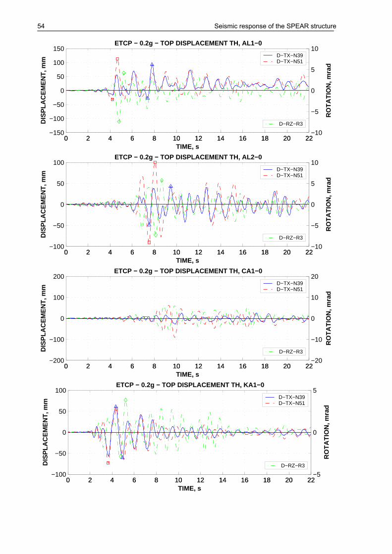
54 Seismic response of the SPEAR structure
0 2 4 6 8 10 12 14 16 18 20 22−150
−100
−50
0
50
100
150
TIME, s
DIS
PL
AC
EM
EN
T, m
mETCP − 0.2g − TOP DISPLACEMENT TH, AL1−0
D−TX−N39 D−TX−N51
0 2 4 6 8 10 12 14 16 18 20 22−10
−5
0
5
10
RO
TA
TIO
N, m
rad
D−RZ−R3
0 2 4 6 8 10 12 14 16 18 20 22−100
−50
0
50
100
TIME, s
DIS
PL
AC
EM
EN
T, m
m
ETCP − 0.2g − TOP DISPLACEMENT TH, AL2−0
D−TX−N39 D−TX−N51
0 2 4 6 8 10 12 14 16 18 20 22−10
−5
0
5
10
RO
TA
TIO
N, m
rad
D−RZ−R3
0 2 4 6 8 10 12 14 16 18 20 22−200
−100
0
100
200
TIME, s
DIS
PL
AC
EM
EN
T, m
m
ETCP − 0.2g − TOP DISPLACEMENT TH, CA1−0
D−TX−N39 D−TX−N51
0 2 4 6 8 10 12 14 16 18 20 22−20
−10
0
10
20
RO
TA
TIO
N, m
rad
D−RZ−R3
0 2 4 6 8 10 12 14 16 18 20 22−100
−50
0
50
100
TIME, s
DIS
PL
AC
EM
EN
T, m
m
ETCP − 0.2g − TOP DISPLACEMENT TH, KA1−0
D−TX−N39 D−TX−N51
0 2 4 6 8 10 12 14 16 18 20 22−5
0
5
RO
TA
TIO
N, m
rad
D−RZ−R3

Seismic response of the SPEAR structure 55
0 2 4 6 8 10 12 14 16 18 20 22−100
−50
0
50
100
TIME, s
DIS
PL
AC
EM
EN
T, m
m
ETCP − 0.2g − TOP DISPLACEMENT TH, KA2−0
D−TX−N39 D−TX−N51
0 2 4 6 8 10 12 14 16 18 20 22−4
−2
0
2
4
RO
TA
TIO
N, m
rad
D−RZ−R3
0 2 4 6 8 10 12 14 16 18 20 22−50
0
50
TIME, s
DIS
PL
AC
EM
EN
T, m
m
ETCP − 0.2g − TOP DISPLACEMENT TH, MO1−0
D−TX−N39 D−TX−N51
0 2 4 6 8 10 12 14 16 18 20 22−5
0
5
RO
TA
TIO
N, m
rad
D−RZ−R3
0 2 4 6 8 10 12 14 16 18 20 22−200
−100
0
100
200
TIME, s
DIS
PL
AC
EM
EN
T, m
m
ETCP − 0.2g − TOP DISPLACEMENT TH, MO2−0
D−TX−N39 D−TX−N51
0 2 4 6 8 10 12 14 16 18 20 22−10
−5
0
5
10
RO
TA
TIO
N, m
rad
D−RZ−R3
Figure 5-36. Time histories of top twist and top displacements in the X direction at the
stiff (N39) and flexible (N51) edges, ETCP model, 0.2g intensity level.

56 Seismic response of the SPEAR structure
0 2 4 6 8 10 12 14 16 18 20 22−100
−50
0
50
100
TIME, s
DIS
PL
AC
EM
EN
T, m
mETCP − 0.2g − TOP DISPLACEMENT TH, AL1−0
D−TY−N39 D−TY−N51
0 2 4 6 8 10 12 14 16 18 20 22−10
−5
0
5
10
RO
TA
TIO
N, m
rad
D−RZ−R3
0 2 4 6 8 10 12 14 16 18 20 22
−50
0
50
TIME, s
DIS
PL
AC
EM
EN
T, m
m
ETCP − 0.2g − TOP DISPLACEMENT TH, AL2−0
D−TY−N39 D−TY−N51
0 2 4 6 8 10 12 14 16 18 20 22
−5
0
5
RO
TA
TIO
N, m
rad
D−RZ−R3
0 2 4 6 8 10 12 14 16 18 20 22−100
−50
0
50
100
TIME, s
DIS
PL
AC
EM
EN
T, m
m
ETCP − 0.2g − TOP DISPLACEMENT TH, CA1−0
D−TY−N39 D−TY−N51
0 2 4 6 8 10 12 14 16 18 20 22−20
−10
0
10
20
RO
TA
TIO
N, m
rad
D−RZ−R3
0 2 4 6 8 10 12 14 16 18 20 22−150
−100
−50
0
50
100
150
TIME, s
DIS
PL
AC
EM
EN
T, m
m
ETCP − 0.2g − TOP DISPLACEMENT TH, KA1−0
D−TY−N39 D−TY−N51
0 2 4 6 8 10 12 14 16 18 20 22−4
−2
0
2
4
RO
TA
TIO
N, m
rad
D−RZ−R3
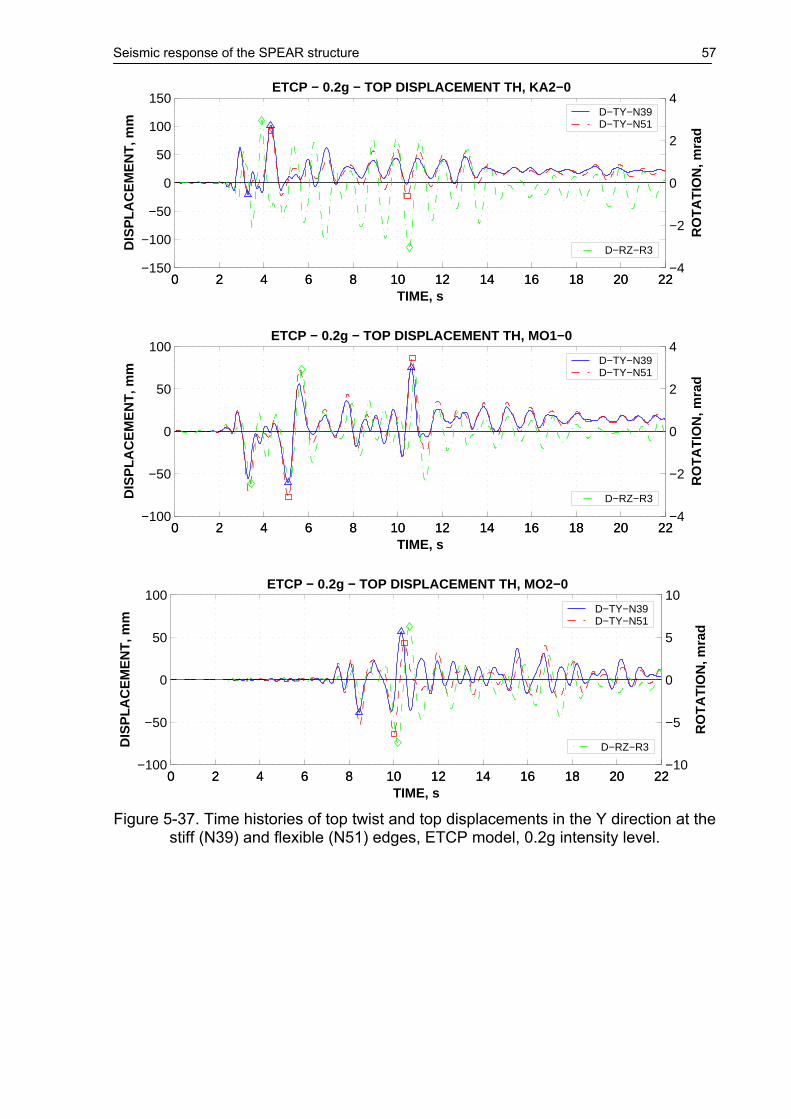
Seismic response of the SPEAR structure 57
0 2 4 6 8 10 12 14 16 18 20 22−150
−100
−50
0
50
100
150
TIME, s
DIS
PL
AC
EM
EN
T, m
m
ETCP − 0.2g − TOP DISPLACEMENT TH, KA2−0
D−TY−N39 D−TY−N51
0 2 4 6 8 10 12 14 16 18 20 22−4
−2
0
2
4
RO
TA
TIO
N, m
rad
D−RZ−R3
0 2 4 6 8 10 12 14 16 18 20 22−100
−50
0
50
100
TIME, s
DIS
PL
AC
EM
EN
T, m
m
ETCP − 0.2g − TOP DISPLACEMENT TH, MO1−0
D−TY−N39 D−TY−N51
0 2 4 6 8 10 12 14 16 18 20 22−4
−2
0
2
4
RO
TA
TIO
N, m
rad
D−RZ−R3
0 2 4 6 8 10 12 14 16 18 20 22−100
−50
0
50
100
TIME, s
DIS
PL
AC
EM
EN
T, m
m
ETCP − 0.2g − TOP DISPLACEMENT TH, MO2−0
D−TY−N39 D−TY−N51
0 2 4 6 8 10 12 14 16 18 20 22−10
−5
0
5
10
RO
TA
TIO
N, m
rad
D−RZ−R3
Figure 5-37. Time histories of top twist and top displacements in the Y direction at the
stiff (N39) and flexible (N51) edges, ETCP model, 0.2g intensity level.

58 Seismic response of the SPEAR structure
0 2 4 6 8 10 12 14 16 18 20 22−200
−100
0
100
200
TIME, s
DIS
PL
AC
EM
EN
T, m
mEFCP − 0.2g − TOP DISPLACEMENT TH, AL1−0
D−TX−N39 D−TX−N51
0 2 4 6 8 10 12 14 16 18 20 22−10
−5
0
5
10
RO
TA
TIO
N, m
rad
D−RZ−R3
0 2 4 6 8 10 12 14 16 18 20 22−200
−100
0
100
200
TIME, s
DIS
PL
AC
EM
EN
T, m
m
EFCP − 0.2g − TOP DISPLACEMENT TH, AL2−0
D−TX−N39 D−TX−N51
0 2 4 6 8 10 12 14 16 18 20 22−10
−5
0
5
10
RO
TA
TIO
N, m
rad
D−RZ−R3
0 2 4 6 8 10 12 14 16 18 20 22−200
−100
0
100
200
TIME, s
DIS
PL
AC
EM
EN
T, m
m
EFCP − 0.2g − TOP DISPLACEMENT TH, CA1−0
D−TX−N39 D−TX−N51
0 2 4 6 8 10 12 14 16 18 20 22−20
−10
0
10
20
RO
TA
TIO
N, m
rad
D−RZ−R3
0 2 4 6 8 10 12 14 16 18 20 22−200
−100
0
100
200
TIME, s
DIS
PL
AC
EM
EN
T, m
m
EFCP − 0.2g − TOP DISPLACEMENT TH, KA1−0
D−TX−N39 D−TX−N51
0 2 4 6 8 10 12 14 16 18 20 22−10
−5
0
5
10
RO
TA
TIO
N, m
rad
D−RZ−R3
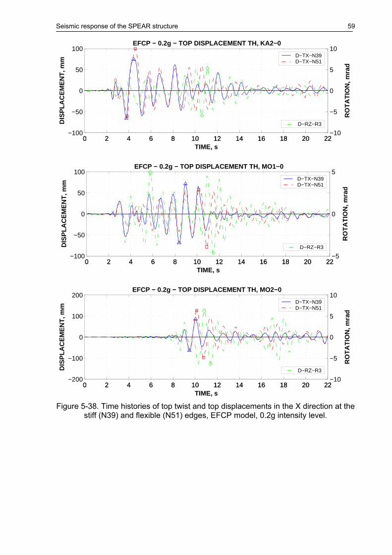
Seismic response of the SPEAR structure 59
0 2 4 6 8 10 12 14 16 18 20 22−100
−50
0
50
100
TIME, s
DIS
PL
AC
EM
EN
T, m
m
EFCP − 0.2g − TOP DISPLACEMENT TH, KA2−0
D−TX−N39 D−TX−N51
0 2 4 6 8 10 12 14 16 18 20 22−10
−5
0
5
10
RO
TA
TIO
N, m
rad
D−RZ−R3
0 2 4 6 8 10 12 14 16 18 20 22−100
−50
0
50
100
TIME, s
DIS
PL
AC
EM
EN
T, m
m
EFCP − 0.2g − TOP DISPLACEMENT TH, MO1−0
D−TX−N39 D−TX−N51
0 2 4 6 8 10 12 14 16 18 20 22−5
0
5
RO
TA
TIO
N, m
rad
D−RZ−R3
0 2 4 6 8 10 12 14 16 18 20 22−200
−100
0
100
200
TIME, s
DIS
PL
AC
EM
EN
T, m
m
EFCP − 0.2g − TOP DISPLACEMENT TH, MO2−0
D−TX−N39 D−TX−N51
0 2 4 6 8 10 12 14 16 18 20 22−10
−5
0
5
10
RO
TA
TIO
N, m
rad
D−RZ−R3
Figure 5-38. Time histories of top twist and top displacements in the X direction at the
stiff (N39) and flexible (N51) edges, EFCP model, 0.2g intensity level.

60 Seismic response of the SPEAR structure
0 2 4 6 8 10 12 14 16 18 20 22−100
−50
0
50
100
TIME, s
DIS
PL
AC
EM
EN
T, m
mEFCP − 0.2g − TOP DISPLACEMENT TH, AL1−0
D−TY−N39 D−TY−N51
0 2 4 6 8 10 12 14 16 18 20 22−10
−5
0
5
10
RO
TA
TIO
N, m
rad
D−RZ−R3
0 2 4 6 8 10 12 14 16 18 20 22−100
−50
0
50
100
TIME, s
DIS
PL
AC
EM
EN
T, m
m
EFCP − 0.2g − TOP DISPLACEMENT TH, AL2−0
D−TY−N39 D−TY−N51
0 2 4 6 8 10 12 14 16 18 20 22−10
−5
0
5
10
RO
TA
TIO
N, m
rad
D−RZ−R3
0 2 4 6 8 10 12 14 16 18 20 22−200
−100
0
100
200
TIME, s
DIS
PL
AC
EM
EN
T, m
m
EFCP − 0.2g − TOP DISPLACEMENT TH, CA1−0
D−TY−N39 D−TY−N51
0 2 4 6 8 10 12 14 16 18 20 22−20
−10
0
10
20
RO
TA
TIO
N, m
rad
D−RZ−R3
0 2 4 6 8 10 12 14 16 18 20 22−200
−100
0
100
200
TIME, s
DIS
PL
AC
EM
EN
T, m
m
EFCP − 0.2g − TOP DISPLACEMENT TH, KA1−0
D−TY−N39 D−TY−N51
0 2 4 6 8 10 12 14 16 18 20 22−10
−5
0
5
10
RO
TA
TIO
N, m
rad
D−RZ−R3
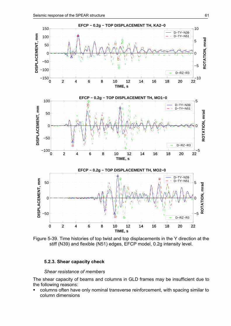
Seismic response of the SPEAR structure 61
0 2 4 6 8 10 12 14 16 18 20 22−150
−100
−50
0
50
100
150
TIME, s
DIS
PL
AC
EM
EN
T, m
m
EFCP − 0.2g − TOP DISPLACEMENT TH, KA2−0
D−TY−N39 D−TY−N51
0 2 4 6 8 10 12 14 16 18 20 22−10
−5
0
5
10
RO
TA
TIO
N, m
rad
D−RZ−R3
0 2 4 6 8 10 12 14 16 18 20 22−100
−50
0
50
100
TIME, s
DIS
PL
AC
EM
EN
T, m
m
EFCP − 0.2g − TOP DISPLACEMENT TH, MO1−0
D−TY−N39 D−TY−N51
0 2 4 6 8 10 12 14 16 18 20 22−5
0
5
RO
TA
TIO
N, m
rad
D−RZ−R3
0 2 4 6 8 10 12 14 16 18 20 22
−50
0
50
TIME, s
DIS
PL
AC
EM
EN
T, m
m
EFCP − 0.2g − TOP DISPLACEMENT TH, MO2−0
D−TY−N39 D−TY−N51
0 2 4 6 8 10 12 14 16 18 20 22
−5
0
5
RO
TA
TIO
N, m
rad
D−RZ−R3
Figure 5-39. Time histories of top twist and top displacements in the Y direction at the
stiff (N39) and flexible (N51) edges, EFCP model, 0.2g intensity level.
5.2.3. Shear capacity check
Shear resistance of members The shear capacity of beams and columns in GLD frames may be insufficient due to the following reasons: columns often have only nominal transverse reinforcement, with spacing similar to
column dimensions

62 Seismic response of the SPEAR structure
beam shear reinforcement is usually in the form of inclined bars, that do not provide a resisting mechanism at load reversal
stirrups may not be adequately anchored with 135° hooks, their efficiency being reduced in this case
Shear capacity of reinforced concrete members is known to depend on the degree of flexural ductility in the plastic hinge. A distinction can be made between a brittle shear failure of columns before the flexural strength of the column has been reached, and ductile shear failure, where a degree of ductility develops in plastic hinges before shear failure occurs. The predictive model for shear strength of r.c. elements proposed by Priestley et al. (1994) is used in this study. It consist of three independent components: a concrete component Vc whose magnitude depends on the level of ductility, an axial load component Vp whose magnitude depends on the column aspect ratio, and a truss component Vs whose magnitude depends on the transverse reinforcement content.
Rd c p sV V V V= + + (5-1)
with the three components evaluated as:
0.8c c gV k f A= ⋅ ⋅ ⋅ (5-2)
k=0.29 for member displacement ductility 1θµ ≤ (biaxial), or curvature ductility 1ϕµ ≤ ; k=0.1 for member displacement ductility 3θµ ≥ (biaxial), or curvature ductility 5ϕµ ≥ ; k varies linearly between member displacement ductility 1 and 3 (see Figure 5-40).
2p
h cV Pa−
= (5-3)
h – the overall section depth; c – the depth of the compression zone; a = L for a cantilever column, and a = L/2 for a column in reversed bending.
cot30sw yws
A f dV
s⋅ ⋅
= ⋅ ° (5-4)
Asw – the total transverse reinforcement area per layer; fyw – the steel yield strength; s – spacing of stirrups; d – the effective depth
Figure 5-40. Degradation of concrete shear strength with ductility,
(Priestley et al., 1994) The model of Priestley et al. (1994) was developed for column sections. The following adjustments have been proposed for evaluation Vc in the case of beams

Seismic response of the SPEAR structure 63
(Priestley, 1997): k=0.2 for member displacement ductility 1θµ ≤ (biaxial), or curvature ductility 1ϕµ ≤ ; k=0.05 for member displacement ductility 3θµ ≥ (biaxial), or curvature ductility 5ϕµ ≥ ; k varies linearly between member displacement ductility 1 and 3. Even if the spacing of stirrups is large in comparison with the column dimensions, steel component was considered for all columns due to the 30° angle between the shear reinforcement and the tension chord in this model. For beams, two shear capacities were computed, corresponding to negative bending (
RdVM − ) when the
inclined reinforcement is effective ( siV ), and corresponding to positive bending (Rd
VM + ), when the inclined reinforcement is ineffective. The following equations apply for different elements of the SPEAR structure: beams:
RdVM
c s siV V V− = + + , Rd
VMc sV V+ = +
columns: Rd
V c s pV V V= + +
Table 5-2. Shear capacity (VRd) and demands (VSd) for selected beams and columns.
Element VRd, kN for µθ=1 (µθ=3) VSd, kN (ETCP, 0.2g) C3 (250x250) 174.3 (116.1) 35.0 C23 (250x250) 145.4 (87.2) 12.5 C6x (250x750) 341.3 (166.9) 39.1 C6y (250x750) 475.1 (300.7) 119.6 C15x (250x750) 334.4 (160.0) 35.6 C15y (250x750) 464.9 (279.4) 98.3 C24x (250x750) 327.5 (153.1) 23.7 C24y (250x750) 453.8 (279.4) 66.7 B1, B2, B3, B5,
B6, B8, B10, B11, B12
MRdV
− = 327.1 (235.3) MRdV
+ = 266.8 (175.0) 60.3
B4, B7, B9, B14 MRdV
− = 434.2 (342.4) MRdV
+ = 266.8 (175.0) 88.1
B13 MRdV
− = 561.5 (469.7) MRdV
+ = 266.8 (175.0) 108.5
The shear force demands for ETCP model at 0.2g earthquake intensity level and capacities for characteristic elements are presented in Figure 5-7. A significant safety margin over shear failure can be observed, indicating that shear failure of elements is not likely to occur, even for higher earthquake intensity levels.
Beam-column joints Shear failure of beam-column joint cores without transverse reinforcement is due to extensive diagonal tension cracking that may eventually lead to diagonal compression failure in the joint core (Hakuto et al., 2000). Attempts have been made to predict the shear failure of the joints by limiting the nominal stress vjh as a function of concrete compressive strength (fc), tensile strength ( cf ), or by limiting the principal compression and tensile stresses in the joint. Two mechanisms of shear resistance are traditionally considered (Paulay and Priestley, 1992): the diagonal strut mechanism and the truss mechanism. The latter is ineffective in the case of

64 Seismic response of the SPEAR structure
joints lacking transverse reinforcement or after bond deterioration between the beam longitudinal reinforcement and the joint core. Consequently, the shear resistance of GLD frames beam-column joints will rely on the diagonal strut mechanism only (see Figure 5-41).
Mb1Mb2
Vc
Figure 5-41. Concrete diagonal strut mechanism in interior bam-column joints.
In the case of exterior beam-column joints, the extent to which the diagonal compression strut mechanism can be mobilised depends greatly on the detailing of longitudinal beam reinforcement. Longitudinal beam reinforcement bent into the joint core (see Figure 5-42a) will permit the diagonal compression strut to bear effectively against the bend, since the bearing stresses at the bend of the bar act in the direction of the strut. When beam reinforcement is bent away from the joint (see Figure 5-42b), diagonal strut in the joint can not be stabilized, and joint failure occurs at an early stage (Priestley, 1997).
(a) (b)
Figure 5-42. Mechanism of shear transfer in exterior beam-column joints. A detailed overview of different provisions for determination of shear capacity of beam-column joints is presented in Stratan and Fajfar, 2002. Joint shear strength predictions according to different approaches differed sometimes by more than 100%. The relatively more conservative provisions of FEMA356 (2000) are used in the present study for estimation of joint shear capacity:
jh cv fλ γ≤ ⋅ (5-5)

Seismic response of the SPEAR structure 65
where λ = 0.75 for lightweight aggregate concrete and 1.0 for normal weight aggregate concrete, and γ is as defined in Table 5-3. In addition to classification of beam-columns joints as interior or exterior, FEMA 356 distinguishes another category of knee joints. The tabulated γ values were interpolated for the case of transverse beams framing into one side of the joint only.
Table 5-3. Values of γ for joint strength calculation, for fc in N/mm2, and ρ"<0.003, FEMA 356, (2000).
Interior joint with transverse beams
Interior joint without transverse beams
Exterior joint with transverse beams
Exterior joint without transverse beams
Knee joint
1.0 0.83 0.66 0.50 0.33
ρ" - volumetric ratio of horizontal confinement reinforcement in the joint; knee joint = self-descriptive (with transverse beams or not).
Table 5-4. Joint shear demand (vjh,Sd), capacity (vjh,Rd), and DCR values for the X direction.
Joint ID
Joint type
vjh,Sd, N/mm2 ETCP, 0.2g
vjh,Rd, N/mm2 DCR
J1-x int. 2.21 5.57 0.40 J2-x ext. 2.28 3.55 0.64 J3-x ext. 2.92 4.04 0.72 J4-x ext. 2.70 3.55 0.76 J5-x ext. 1.65 3.55 0.46 J6-x int. 1.08 5.57 0.19 J7-x ext. 2.06 3.55 0.58 J8-x ext. 1.48 3.55 0.42 J9-x ext. 2.36 4.04 0.58 J10-x int. 1.70 5.57 0.30 J11-x ext. 1.68 3.55 0.47 J12-x ext. 2.30 4.04 0.57 J13-x ext. 2.09 3.55 0.59 J14-x ext. 1.26 3.55 0.35 J15-x int. 0.88 5.57 0.16 J16-x ext. 1.19 3.55 0.34 J17-x ext. 1.07 3.55 0.30 J18-x ext. 1.76 4.04 0.44 J19-x int. 0.87 5.57 0.16 J20-x ext. 0.76 2.02 0.38 J21-x ext. 1.60 2.02 0.79 J22-x ext. 1.12 2.02 0.56 J23-x ext. 0.63 2.02 0.31 J24-x int. 0.47 5.57 0.08 J25-x ext. 0.75 2.02 0.37 J26-x ext. 0.63 2.02 0.31 J27-x ext. 1.00 2.02 0.49

66 Seismic response of the SPEAR structure
Table 5-5. Joint shear demand (vjh,Sd), capacity (vjh,Rd), and DCR values for the Y direction.
Joint ID
Joint type
vjh,Sd, N/mm2 ETCP, 0.2g
vjh,Rd, N/mm2 DCR
J1-y ext. 2.23 4.04 0.55 J2-y ext. 2.29 3.55 0.64 J3-y int. 2.61 5.57 0.47 J4-y ext. 1.73 3.55 0.49 J5-y ext. 1.21 3.55 0.34 J6-y ext. 1.15 3.06 0.37 J7-y ext. 2.62 3.55 0.74 J8-y ext. 2.35 3.55 0.66 J9-y int. 1.87 5.57 0.34
J10-y ext. 1.87 4.04 0.46 J11-y ext. 1.82 3.55 0.51 J12-y int. 2.11 5.57 0.38 J13-y ext. 1.36 3.55 0.38 J14-y ext. 1.04 3.55 0.29 J15-y ext. 1.20 3.06 0.39 J16-y ext. 2.20 3.55 0.62 J17-y ext. 2.00 3.55 0.56 J18-y int. 1.64 5.57 0.29 J19-y ext. 0.97 2.02 0.48 J20-y ext. 0.93 2.02 0.46 J21-y int. 1.02 5.57 0.18 J22-y ext. 0.94 2.02 0.47 J23-y ext. 0.55 2.02 0.27 J24-y ext. 1.16 2.02 0.58 J25-y ext. 1.05 2.02 0.52 J26-y ext. 1.00 2.02 0.49 J27-y int. 0.90 5.57 0.16
Joint shear demands (mean of dynamic analyses for 0.2g seismic intensity level, ETCP model), capacities according to FEMA356 approach, and the DCRs are presented in Table 5-4 and Table 5-5. As in case of element shear capacity, a sufficient safety margin exists between the demand and capacity that shows little chance for joint shear failure.
5.3. Earthquake intensity level 0.1g
5.3.1. Pushover analysis
Pushover curves for the ETCP and EFCP models with displacement demands determined by N2 method for the 0.1g PGA are presented in Figure 5-43 and Figure 5-44. Though some degree of yielding is experienced by structural members, the global structural yield is not attained.

Seismic response of the SPEAR structure 67
−200 −150 −100 −50 0 50 100 150 2000
50
100
150
200
250
300
TOP DISPLACEMENT, mm
BA
SE
SH
EA
R, k
N
MODE1
ETCP−100XEFCP−100X1st yieldN2 DEMAND
Figure 5-43. Comparison of pushover curves in the X directions for ETCP and EFCP
models, displacement demands for 0.1g intensity level.
−200 −150 −100 −50 0 50 100 150 2000
50
100
150
200
250
300
350
400
TOP DISPLACEMENT, mm
BA
SE
SH
EA
R, k
N
MODE1
ETCP−100YEFCP−100Y1st yieldN2 DEMAND
Figure 5-44. Comparison of pushover curves in the X directions for ETCP and EFCP
models, displacement demands for 0.1g intensity level.
5.3.2. Dynamic analysis
Predictions of top displacement and twist demands for the 0.1g earthquake intensity level are presented in Figure 5-45 and Figure 5-46 for the ETCP and EFCP models respectively. Similarly to the 0.2g intensity level, higher displacement demands are

68 Seismic response of the SPEAR structure
present at the flexible edge than at the stiff edge, and the torsional amplifications of displacement demands at the flexible edge are higher for the X direction. Unsymmetrical displacement demands in the positive and negative senses of the Y direction are noted for this lower intensity level, indicating that it is attributed not only to the strength, but also to the stiffness asymmetry. Distribution of interstorey drifts along the height of the building is similar to the one under 0.2g seismic input for the Y direction, relatively uniform drift demands being observed for the three storeys. In the X direction a different response is observed. Interstorey drift demands are uniform along the height of the building at the centre of mass and at the stiff edge for the low intensity level. However, at the flexible edge a concentration of drift demands in the lower storey is observed, similarly to the 0.2g seismic input (see Figure 5-47 and Figure 5-10). This can be explained by observing the ductility demand plots for the ETCP model in Figure 5-48. Column yielding is noted only for the lower two storeys at the flexible edge, which causes an increase of drift demands in the lower part of the building. Extensive yielding of beams under positive bending moments is present (pullout of beam bottom bars). Additionally, plastic deformations are present at the bottom of the 250x750 column for bending in the strong direction, and for the B10 beam at the interface with the 250x750 column (under negative bending). Ductility demands of the EFCP model show yielding of reinforcement in several columns, with higher ductility demands for the base of the strong C6 column and the “flexible edge” C1, C2, C5, C10, C11, C14 columns. Concrete crushing is not present at this level of seismic input. Due to higher displacement demands, the B24 beam yields under negative moment in addition to the B10 beam. Sample moment-rotation and moment-curvature response of the beam B1, and columns C2 and C3 for the ETCP and EFCP models are presented in Figure 5-49 through Figure 5-52.
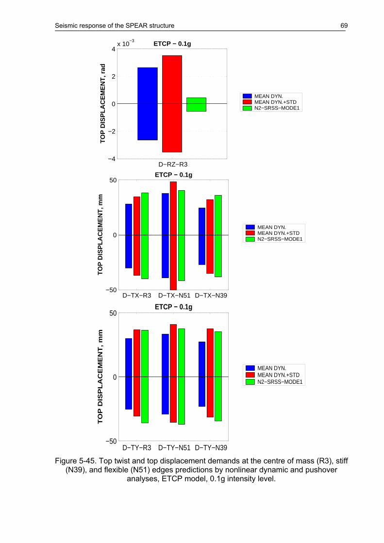
Seismic response of the SPEAR structure 69
D−RZ−R3−4
−2
0
2
4x 10
−3
TO
P D
ISP
LA
CE
ME
NT
, rad
ETCP − 0.1g
MEAN DYN.MEAN DYN.+STDN2−SRSS−MODE1
D−TX−R3 D−TX−N51 D−TX−N39−50
0
50
TO
P D
ISP
LA
CE
ME
NT
, mm
ETCP − 0.1g
MEAN DYN.MEAN DYN.+STDN2−SRSS−MODE1
D−TY−R3 D−TY−N51 D−TY−N39−50
0
50
TO
P D
ISP
LA
CE
ME
NT
, m
m
ETCP − 0.1g
MEAN DYN.MEAN DYN.+STDN2−SRSS−MODE1
Figure 5-45. Top twist and top displacement demands at the centre of mass (R3), stiff
(N39), and flexible (N51) edges predictions by nonlinear dynamic and pushover analyses, ETCP model, 0.1g intensity level.

70 Seismic response of the SPEAR structure
D−RZ−R3−6
−4
−2
0
2
4
6x 10
−3
TO
P D
ISP
LA
CE
ME
NT
, rad
EFCP − 0.1g
MEAN DYN.MEAN DYN.+STDN2−SRSS−MODE1
D−TX−R3 D−TX−N51 D−TX−N39−80
−60
−40
−20
0
20
40
60
80
TO
P D
ISP
LA
CE
ME
NT
, m
m
EFCP − 0.1g
MEAN DYN.MEAN DYN.+STDN2−SRSS−MODE1
D−TY−R3 D−TY−N51 D−TY−N39−50
0
50
TO
P D
ISP
LA
CE
ME
NT
, mm
EFCP − 0.1g
MEAN DYN.MEAN DYN.+STDN2−SRSS−MODE1
Figure 5-46. Top twist and top displacement demands at the centre of mass (R3), stiff
(N39), and flexible (N51) edges predictions by nonlinear dynamic and pushover analyses, EFCP model, 0.1g intensity level.

Seismic response of the SPEAR structure 71
−6 −4 −2 0 2 4 6
x 10−3
0
2
4
6
8
10
TX, rad
HE
IGH
T, m
MEAN DYNAMIC − 0.1g − CM
ETCPEFCP
−5 0 5
x 10−3
0
2
4
6
8
10
TY, rad
HE
IGH
T, m
MEAN DYNAMIC − 0.1g − CM
ETCPEFCP
−6 −4 −2 0 2 4 6
x 10−3
0
2
4
6
8
10
TX, rad
HE
IGH
T, m
MEAN DYNAMIC − 0.1g − X1Y1
ETCPEFCP
−5 0 5
x 10−3
0
2
4
6
8
10
TY, rad
HE
IGH
T, m
MEAN DYNAMIC − 0.1g − X1Y1
ETCPEFCP
−5 0 5
x 10−3
0
2
4
6
8
10
TX, rad
HE
IGH
T, m
MEAN DYNAMIC − 0.1g − X3Y3
ETCPEFCP
−6 −4 −2 0 2 4 6
x 10−3
0
2
4
6
8
10
TY, rad
HE
IGH
T, m
MEAN DYNAMIC − 0.1g − X3Y3
ETCPEFCP
Figure 5-47. Comparison of interstorey drift demands for the ETCP and EFCP
models, 0.1g intensity level at the centre of mass (CM), stiff (X1Y1), and flexible (X3Y3) edges.

72 Seismic response of the SPEAR structure
0 2 4 6 8 10
0
2
4
6
8
ETCP − 0.1g − ductility demands − X1
X
Z
0 2 4 6 8 10
0
2
4
6
8
ETCP − 0.1g − ductility demands − X2
X
Z
0 2 4 6 8 10
0
2
4
6
8
ETCP − 0.1g − ductility demands − X3
X
Z
0 2 4 6 8 10 12
0
2
4
6
8
ETCP − 0.1g − ductility demands − Y1
Y
Z
0 2 4 6 8 10 12
0
2
4
6
8
ETCP − 0.1g − ductility demands − Y2
Y
Z
0 2 4 6 8 10 12
0
2
4
6
8
ETCP − 0.1g − ductility demands − Y3
Y
Z
Figure 5-48. Mean dynamic rotation/curvature ductility demands in elements,
ETCP model, 0.1g intensity level.

Seismic response of the SPEAR structure 73
−0.02 −0.01 0 0.01 0.02−60
−40
−20
0
20
40
60
L − ROTATION, rad
MO
ME
NT
, kN
m
ETCP − 0.1g − B1 − AL1−0
−0.02 −0.01 0 0.01 0.02−60
−40
−20
0
20
40
60
L − ROTATION, rad
MO
ME
NT
, kN
m
ETCP − 0.1g − B1 − AL2−0
Figure 5-49. Moment-rotation history for the beam B1 left end (i), ETCP model, AL1-0
and AL2-0 records, 0.1g intensity level.
−0.02 −0.01 0 0.01 0.02−60
−40
−20
0
20
40
60
L − ROTATION, rad
MO
ME
NT
, kN
m
EFCP − 0.1g − B1 − AL1−0
−0.02 −0.01 0 0.01 0.02−60
−40
−20
0
20
40
60
L − ROTATION, rad
MO
ME
NT
, kN
mEFCP − 0.1g − B1 − AL2−0
Figure 5-50. Moment-rotation history for the beam B1 left end (i), EFCP model, AL1-0
and AL2-0 records, 0.1g intensity level.
−0.02 −0.01 0 0.01 0.02
−60
−40
−20
0
20
40
60
Mx1 − ROTATION, rad
MO
ME
NT
, kN
m
ETCP − 0.1g − C2 − AL1−0
−0.02 −0.01 0 0.01 0.02
−60
−40
−20
0
20
40
60
My1 − ROTATION, rad
MO
ME
NT
, kN
m
ETCP − 0.1g − C2 − AL1−0

74 Seismic response of the SPEAR structure
−0.02 −0.01 0 0.01 0.02
−60
−40
−20
0
20
40
60
Mx1 − ROTATION, rad
MO
ME
NT
, kN
mETCP − 0.1g − C2 − AL2−0
−0.02 −0.01 0 0.01 0.02
−60
−40
−20
0
20
40
60
My1 − ROTATION, rad
MO
ME
NT
, kN
m
ETCP − 0.1g − C2 − AL2−0
Figure 5-51. Moment-rotation history for the column C2 bottom end, ETCP model,
AL1-0 and AL2-0 records, 0.1g intensity level.
−0.06 −0.04 −0.02 0 0.02 0.04
−60
−40
−20
0
20
40
60
Mx1 − CURVATURE, 1/m
MO
ME
NT
, kN
m
EFCP − 0.1g − C2 − AL1−0
−0.06 −0.04 −0.02 0 0.02 0.04
−60
−40
−20
0
20
40
60
My1 − CURVATURE, 1/m
MO
ME
NT
, kN
m
EFCP − 0.1g − C2 − AL1−0
−0.06 −0.04 −0.02 0 0.02 0.04
−60
−40
−20
0
20
40
60
Mx1 − CURVATURE, 1/m
MO
ME
NT
, kN
m
EFCP − 0.1g − C2 − AL2−0
−0.06 −0.04 −0.02 0 0.02 0.04
−60
−40
−20
0
20
40
60
My1 − CURVATURE, 1/m
MO
ME
NT
, kN
m
EFCP − 0.1g − C2 − AL2−0
Figure 5-52. Moment-rotation history for the column C2 bottom end, EFCP model,
AL1-0 and AL2-0 records, 0.1g intensity level.

Seismic response of the SPEAR structure 75
5.4. Earthquake intensity level 0.3g
5.4.1. Pushover analysis
Pushover curves for the ETCP and EFCP models with displacement demands determined by N2 method for the 0.3g PGA are presented in Figure 5-53 and Figure 5-54. Higher displacement demands are noted for the more flexible EFCP model, similarly to the 0.2g earthquake intensity level. However, for 0.3g PGA, the structure approaches failure (as predicted by the pushover analysis), global strength degradation following at larger displacement demands. Strength degradation is higher in the X direction.
−200 −150 −100 −50 0 50 100 150 2000
50
100
150
200
250
300
TOP DISPLACEMENT, mm
BA
SE
SH
EA
R, k
N
MODE1
ETCP−100XEFCP−100X1st yieldN2 DEMAND
Figure 5-53. Comparison of pushover curves in the X directions for ETCP and EFCP
models, displacement demands for 0.3g intensity level.
−200 −150 −100 −50 0 50 100 150 2000
50
100
150
200
250
300
350
400
TOP DISPLACEMENT, mm
BA
SE
SH
EA
R, k
N
MODE1
ETCP−100YEFCP−100Y1st yieldN2 DEMAND
Figure 5-54. Comparison of pushover curves in the X directions for ETCP and EFCP
models, displacement demands for 0.3g intensity level.

76 Seismic response of the SPEAR structure
5.4.2. Dynamic analysis
Predictions of top displacement and twist demands for the 0.3g earthquake intensity level are presented in Figure 5-55 and Figure 5-56 for the ETCP and EFCP models respectively. The same trends described for the 0.2g intensity level are observed. However, unconservative estimations of top displacements by the N2 method are noted for the both positive and negative Y directions. Distribution of interstorey drifts along the height of the building is similar to the one under 0.2g seismic input for the both X and Y directions (see Figure 5-57). A concentration of displacement demands in the first storey is present at the flexible edge (X3 frame line), especially in the case of the EFCP model (due to M-M-N effects and cyclic stiffness and strength degradation). The yielding pattern of the ETCP model is basically the same as for the 0.2g earthquake intensity level (see Figure 5-58), but additional members experience yielding in the upper storey. Beam and column DCRs for the ETCP model are presented in Figure 5-63. Important damage (DCR>0.5) is observed for beams in the lower storey. With the exception of the B10 and B24 beams framing into the strong 250x750 column, the rest of the beams yield mainly under positive bending (pull-out of bottom reinforcement). Higher DCRs are present for shorter beams (B1,B3, B5) and/or at the exterior beam-column joints. However, all the beams have DCRs less than 1. Column DCRs (Figure 5-64 to Figure 5-67) are higher at the first storey, flexible edge elements. Several columns experience DCRs in excess of 1.0, indicating attainment of rotation capacity and initiation of collapse. Thus, failure of first storey C2, C3 and C4, as well as second storey C12 columns is predicted by the concentrated plasticity ETCP model. In the case of the EFCP model, slightly higher DCRs are present for first storey beams. Collapse of distributed plasticity fibre columns is more difficult to monitor than for the ETCP model. However, significant strength degradation was noted for some first storey columns under particular earthquake records (e.g. C3 column under AL2, CA2, KA2 records). Anyway, mean dynamic strain demands in concrete fibres indicate extensive damage to columns under the 0.3g excitation level. Complete spalling of cover concrete (strain demands over ultimate concrete strains) are present for all first storey columns with the exception of C8. Very high concrete strains are observed for the C2, C3, and C4 columns, which indicate that also core concrete is severely damaged. Spalling of cover concrete for the second storey C10, C11, C12, C13 and C15 columns is also expected, but the integrity of the core concrete may be sufficient to preserve member load-carrying capacity. Low concrete strain demands are present in the third storey columns.

Seismic response of the SPEAR structure 77
D−RZ−R3−0.015
−0.01
−0.005
0
0.005
0.01
0.015
TO
P D
ISP
LA
CE
ME
NT
, rad
ETCP − 0.3g
MEAN DYN.MEAN DYN.+STDN2−SRSS−MODE1
D−TX−R3 D−TX−N51 D−TX−N39−200
−100
0
100
200
TO
P D
ISP
LA
CE
ME
NT
, mm
ETCP − 0.3g
MEAN DYN.MEAN DYN.+STDN2−SRSS−MODE1
D−TY−R3 D−TY−N51 D−TY−N39
−200
−100
0
100
200
TO
P D
ISP
LA
CE
ME
NT
, m
m
ETCP − 0.3g
MEAN DYN.MEAN DYN.+STDN2−SRSS−MODE1
Figure 5-55. Top twist and top displacement demands at the centre of mass (R3), stiff
(N39), and flexible (N51) edges predictions by nonlinear dynamic and pushover analyses, ETCP model, 0.3g intensity level.

78 Seismic response of the SPEAR structure
D−RZ−R3−0.015
−0.01
−0.005
0
0.005
0.01
0.015
TO
P D
ISP
LA
CE
ME
NT
, rad
EFCP − 0.3g
MEAN DYN.MEAN DYN.+STDN2−SRSS−MODE1
D−TX−R3 D−TX−N51 D−TX−N39−200
−100
0
100
200
TO
P D
ISP
LA
CE
ME
NT
, m
m
EFCP − 0.3g
MEAN DYN.MEAN DYN.+STDN2−SRSS−MODE1
D−TY−R3 D−TY−N51 D−TY−N39
−200
−100
0
100
200
TO
P D
ISP
LA
CE
ME
NT
, mm
EFCP − 0.3g
MEAN DYN.MEAN DYN.+STDN2−SRSS−MODE1
Figure 5-56. Top twist and top displacement demands at the centre of mass (R3), stiff
(N39), and flexible (N51) edges predictions by nonlinear dynamic and pushover analyses, EFCP model, 0.3g intensity level.

Seismic response of the SPEAR structure 79
−0.02 −0.01 0 0.01 0.020
2
4
6
8
10
TX, rad
HE
IGH
T, m
MEAN DYNAMIC − 0.3g − CM
ETCPEFCP
−0.02 −0.01 0 0.01 0.020
2
4
6
8
10
TY, rad
HE
IGH
T, m
MEAN DYNAMIC − 0.3g − CM
ETCPEFCP
−0.02 −0.01 0 0.01 0.020
2
4
6
8
10
TX, rad
HE
IGH
T, m
MEAN DYNAMIC − 0.3g − X1Y1
ETCPEFCP
−0.02 −0.01 0 0.01 0.020
2
4
6
8
10
TY, rad
HE
IGH
T, m
MEAN DYNAMIC − 0.3g − X1Y1
ETCPEFCP
−0.02 −0.01 0 0.01 0.020
2
4
6
8
10
TX, rad
HE
IGH
T, m
MEAN DYNAMIC − 0.3g − X3Y3
ETCPEFCP
−0.03 −0.02 −0.01 0 0.01 0.020
2
4
6
8
10
TY, rad
HE
IGH
T, m
MEAN DYNAMIC − 0.3g − X3Y3
ETCPEFCP
Figure 5-57. Comparison of interstorey drift demands for the ETCP and EFCP
models, 0.3g intensity level at the centre of mass (CM), stiff (X1Y1), and flexible (X3Y3) edges.

80 Seismic response of the SPEAR structure
0 2 4 6 8 10
0
2
4
6
8
ETCP − 0.3g − ductility demands − X1
X
Z
0 2 4 6 8 10
0
2
4
6
8
ETCP − 0.3g − ductility demands − X2
X
Z
0 2 4 6 8 10
0
2
4
6
8
ETCP − 0.3g − ductility demands − X3
X
Z
0 2 4 6 8 10 12
0
2
4
6
8
ETCP − 0.3g − ductility demands − Y1
Y
Z
0 2 4 6 8 10 12
0
2
4
6
8
ETCP − 0.3g − ductility demands − Y2
Y
Z
0 2 4 6 8 10 12
0
2
4
6
8
ETCP − 0.3g − ductility demands − Y3
Y
Z
Figure 5-58. Mean dynamic rotation/curvature ductility demands in elements, ETCP
model, 0.3g intensity level.

Seismic response of the SPEAR structure 81
−0.02 −0.01 0 0.01 0.02−60
−40
−20
0
20
40
60
L − ROTATION, rad
MO
ME
NT
, kN
m
ETCP − 0.3g − B1 − AL1−0
−0.02 −0.01 0 0.01 0.02−60
−40
−20
0
20
40
60
L − ROTATION, rad
MO
ME
NT
, kN
m
ETCP − 0.3g − B1 − AL2−0
Figure 5-59. Moment-rotation history for the beam B1 left end (i), ETCP model, AL1-0
and AL2-0 records, 0.3g intensity level.
−0.02 −0.01 0 0.01 0.02−60
−40
−20
0
20
40
60
L − ROTATION, rad
MO
ME
NT
, kN
m
EFCP − 0.3g − B1 − AL1−0
−0.02 −0.01 0 0.01 0.02−60
−40
−20
0
20
40
60
L − ROTATION, rad
MO
ME
NT
, kN
mEFCP − 0.3g − B1 − AL2−0
Figure 5-60. Moment-rotation history for the beam B1 left end (i), EFCP model, AL1-0
and AL2-0 records, 0.3g intensity level.
−0.02 −0.01 0 0.01 0.02
−60
−40
−20
0
20
40
60
Mx1 − ROTATION, rad
MO
ME
NT
, kN
m
ETCP − 0.3g − C2 − AL1−0
−0.02 −0.01 0 0.01 0.02
−60
−40
−20
0
20
40
60
My1 − ROTATION, rad
MO
ME
NT
, kN
m
ETCP − 0.3g − C2 − AL1−0
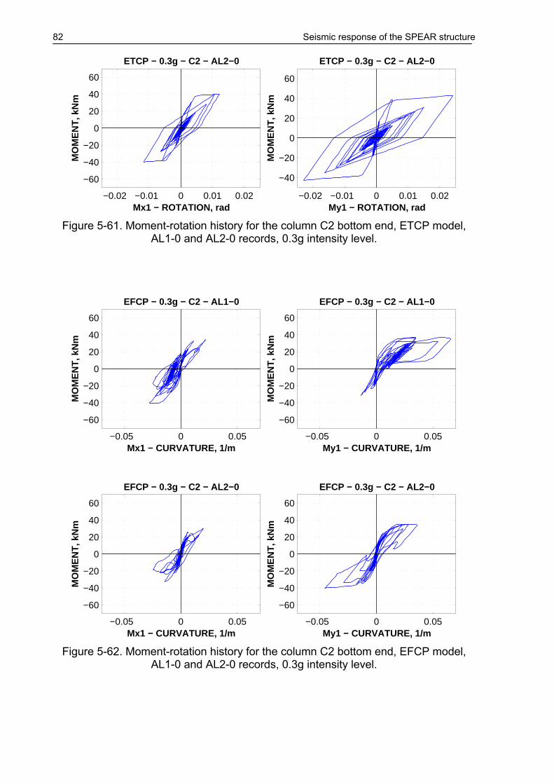
82 Seismic response of the SPEAR structure
−0.02 −0.01 0 0.01 0.02
−60
−40
−20
0
20
40
60
Mx1 − ROTATION, rad
MO
ME
NT
, kN
mETCP − 0.3g − C2 − AL2−0
−0.02 −0.01 0 0.01 0.02
−40
−20
0
20
40
60
My1 − ROTATION, rad
MO
ME
NT
, kN
m
ETCP − 0.3g − C2 − AL2−0
Figure 5-61. Moment-rotation history for the column C2 bottom end, ETCP model,
AL1-0 and AL2-0 records, 0.3g intensity level.
−0.05 0 0.05
−60
−40
−20
0
20
40
60
Mx1 − CURVATURE, 1/m
MO
ME
NT
, kN
m
EFCP − 0.3g − C2 − AL1−0
−0.05 0 0.05
−60
−40
−20
0
20
40
60
My1 − CURVATURE, 1/m
MO
ME
NT
, kN
m
EFCP − 0.3g − C2 − AL1−0
−0.05 0 0.05
−60
−40
−20
0
20
40
60
Mx1 − CURVATURE, 1/m
MO
ME
NT
, kN
m
EFCP − 0.3g − C2 − AL2−0
−0.05 0 0.05
−60
−40
−20
0
20
40
60
My1 − CURVATURE, 1/m
MO
ME
NT
, kN
m
EFCP − 0.3g − C2 − AL2−0
Figure 5-62. Moment-rotation history for the column C2 bottom end, EFCP model,
AL1-0 and AL2-0 records, 0.3g intensity level.

Seismic response of the SPEAR structure 83
B1 B2 B3 B4 B5 B6 B7 B8 B9 B10 B11 B12 B13 B14−1.5
−1
−0.5
0
0.5
1
1.5
L
RO
TA
TIO
N D
CR
ETCP − 0.3g, STOREY 1
DYN. MEAN(MAX)DYN. MEAN + STDN2−SRSS−MODE1
B15 B16 B17 B18 B19 B20 B21 B22 B23 B24 B25 B26 B27 B28−1.5
−1
−0.5
0
0.5
1
1.5
L
RO
TA
TIO
N D
CR
ETCP − 0.3g, STOREY 2
DYN. MEAN(MAX)DYN. MEAN + STDN2−SRSS−MODE1
B29 B30 B31 B32 B33 B34 B35 B36 B37 B38 B39 B40 B41 B42−1.5
−1
−0.5
0
0.5
1
1.5
L
RO
TA
TIO
N D
CR
ETCP − 0.3g, STOREY 3
DYN. MEAN(MAX)DYN. MEAN + STDN2−SRSS−MODE1

84 Seismic response of the SPEAR structure
B1 B2 B3 B4 B5 B6 B7 B8 B9 B10 B11 B12 B13 B14−1.5
−1
−0.5
0
0.5
1
1.5
R
RO
TA
TIO
N D
CR
ETCP − 0.3g, STOREY 1
DYN. MEAN(MAX)DYN. MEAN + STDN2−SRSS−MODE1
B15 B16 B17 B18 B19 B20 B21 B22 B23 B24 B25 B26 B27 B28−1.5
−1
−0.5
0
0.5
1
1.5
R
RO
TA
TIO
N D
CR
ETCP − 0.3g, STOREY 2
DYN. MEAN(MAX)DYN. MEAN + STDN2−SRSS−MODE1
B29 B30 B31 B32 B33 B34 B35 B36 B37 B38 B39 B40 B41 B42−1.5
−1
−0.5
0
0.5
1
1.5
R
RO
TA
TIO
N D
CR
ETCP − 0.3g, STOREY 3
DYN. MEAN(MAX)DYN. MEAN + STDN2−SRSS−MODE1
Figure 5-63. Rotation DCRs in beams, ETCP model, 0.3g intensity level
(L – left [i] end; R – right [j] end).

Seismic response of the SPEAR structure 85
C1 C2 C3 C4 C5 C6 C7 C8 C90
0.5
1
1.5
2
Mx1
RO
TA
TIO
N D
CR
ETCP − 0.3g, STOREY 1
DYN. MEAN(MAX)DYN. MEAN + STDN2−SRSS−MODE1
C10 C11 C12 C13 C14 C15 C16 C17 C180
0.5
1
1.5
2
Mx1
RO
TA
TIO
N D
CR
ETCP − 0.3g, STOREY 2
DYN. MEAN(MAX)DYN. MEAN + STDN2−SRSS−MODE1
C19 C20 C21 C22 C23 C24 C25 C26 C270
0.5
1
1.5
2
Mx1
RO
TA
TIO
N D
CR
ETCP − 0.3g, STOREY 3
DYN. MEAN(MAX)DYN. MEAN + STDN2−SRSS−MODE1
Figure 5-64. DCRs in columns (bending about X axis at the bottom end), ETCP
model, 0.3g intensity level.

86 Seismic response of the SPEAR structure
C1 C2 C3 C4 C5 C6 C7 C8 C90
0.5
1
1.5
2
My1
RO
TA
TIO
N D
CR
ETCP − 0.3g, STOREY 1
DYN. MEAN(MAX)DYN. MEAN + STDN2−SRSS−MODE1
C10 C11 C12 C13 C14 C15 C16 C17 C180
0.5
1
1.5
2
My1
RO
TA
TIO
N D
CR
ETCP − 0.3g, STOREY 2
DYN. MEAN(MAX)DYN. MEAN + STDN2−SRSS−MODE1
C19 C20 C21 C22 C23 C24 C25 C26 C270
0.5
1
1.5
2
My1
RO
TA
TIO
N D
CR
ETCP − 0.3g, STOREY 3
DYN. MEAN(MAX)DYN. MEAN + STDN2−SRSS−MODE1
Figure 5-65. DCRs in columns (bending about Y axis at the bottom end), ETCP
model, 0.3g intensity level.
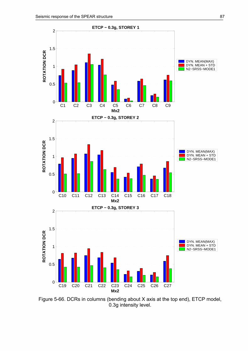
Seismic response of the SPEAR structure 87
C1 C2 C3 C4 C5 C6 C7 C8 C90
0.5
1
1.5
2
Mx2
RO
TA
TIO
N D
CR
ETCP − 0.3g, STOREY 1
DYN. MEAN(MAX)DYN. MEAN + STDN2−SRSS−MODE1
C10 C11 C12 C13 C14 C15 C16 C17 C180
0.5
1
1.5
2
Mx2
RO
TA
TIO
N D
CR
ETCP − 0.3g, STOREY 2
DYN. MEAN(MAX)DYN. MEAN + STDN2−SRSS−MODE1
C19 C20 C21 C22 C23 C24 C25 C26 C270
0.5
1
1.5
2
Mx2
RO
TA
TIO
N D
CR
ETCP − 0.3g, STOREY 3
DYN. MEAN(MAX)DYN. MEAN + STDN2−SRSS−MODE1
Figure 5-66. DCRs in columns (bending about X axis at the top end), ETCP model,
0.3g intensity level.

88 Seismic response of the SPEAR structure
C1 C2 C3 C4 C5 C6 C7 C8 C90
0.5
1
1.5
2
My2
RO
TA
TIO
N D
CR
ETCP − 0.3g, STOREY 1
DYN. MEAN(MAX)DYN. MEAN + STDN2−SRSS−MODE1
C10 C11 C12 C13 C14 C15 C16 C17 C180
0.5
1
1.5
2
My2
RO
TA
TIO
N D
CR
ETCP − 0.3g, STOREY 2
DYN. MEAN(MAX)DYN. MEAN + STDN2−SRSS−MODE1
C19 C20 C21 C22 C23 C24 C25 C26 C270
0.5
1
1.5
2
My2
RO
TA
TIO
N D
CR
ETCP − 0.3g, STOREY 3
DYN. MEAN(MAX)DYN. MEAN + STDN2−SRSS−MODE1
Figure 5-67. DCRs in columns (bending about Y axis at the top end), ETCP model,
0.3g intensity level.

Seismic response of the SPEAR structure 89
5.5. Difference between the response of ETCP and EFCP models
As it was stated earlier, two models were used two assess seismic performance of the SPEAR building. The difference between the two models was column elements modelling (concentrated plasticity one-component elements in the case of ETCP model, and distributed plasticity fibre elements in the case of the EFCP model). The main drawback of the ETCP model is that it does not consider the P-M-M interaction effects, and strength degradation. The EFCP model on the other hand, while representing well these effects is computationally less efficient, and the results are much more difficult to process. The two structural models showed generally a similar response. The EFCP model was however more flexible than the ETCP one, providing higher displacement demands (see Figure 5-10). The shape of the column moment-rotation or moment-curvature hysteresis loops were sometimes quite different for the two models (see Figure 5-32 to Figure 5-35), the fibre model being characterised by pinching and a moderate strength degradation, which resulted in lower energy dissipation. Time history response of the global response parameters (e.g. top displacement) were however similar for the two models (see Figure 5-68). The ETCP model had the advantage of easy and meaningful assessment of element response parameters by DCRs (chord rotation demands are easily compared to empirical or computed rotation capacities). However, the EFCP model had the advantage of more "correct" global response, strength degradation being easily followed on the pushover curves (see Figure 5-3 and Figure 5-4).
0 2 4 6 8 10 12 14 16 18 20 22
−100
−50
0
50
100
TIME, s
D−T
X−R
3, m
m
TOP DISPLACEMENT TH, AL1−0
ETCPEFCP
0 2 4 6 8 10 12 14 16 18 20 22−100
−50
0
50
100
TIME, s
D−T
X−R
3, m
m
TOP DISPLACEMENT TH, AL2−0
ETCPEFCP
Figure 5-68. Top displacement time histories for the ETCP and EFCP models
under the AL1-0 and AL2-0 records.
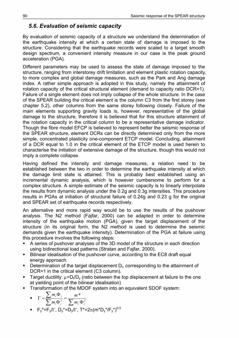
90 Seismic response of the SPEAR structure
5.6. Evaluation of seismic capacity
By evaluation of seismic capacity of a structure we understand the determination of the earthquake intensity at which a certain state of damage is imposed to the structure. Considering that the earthquake records were scaled to a target smooth design spectrum, a convenient intensity measure in our case is the peak ground acceleration (PGA). Different parameters may be used to assess the state of damage imposed to the structure, ranging from interstorey drift limitation and element plastic rotation capacity, to more complex and global damage measures, such as the Park and Ang damage index. A rather simple approach is adopted in this study, namely the attainment of rotation capacity of the critical structural element (demand to capacity ratio DCR=1). Failure of a single element does not imply collapse of the whole structure. In the case of the SPEAR building the critical element is the column C3 from the first storey (see chapter 5.2), other columns from the same storey following closely. Failure of the main elements supporting gravity loads is, however, representative of the global damage to the structure, therefore it is believed that for this structure attainment of the rotation capacity in the critical column to be a representative damage indicator. Though the fibre model EFCP is believed to represent better the seismic response of the SPEAR structure, element DCRs can be directly determined only from the more simple, concentrated plasticity one-component ETCP model. Concluding, attainment of a DCR equal to 1.0 in the critical element of the ETCP model is used herein to characterise the initiation of extensive damage of the structure, though this would not imply a complete collapse. Having defined the intensity and damage measures, a relation need to be established between the two in order to determine the earthquake intensity at which the damage limit state is attained. This is probably best established using an incremental dynamic analysis, which is however cumbersome to perform for a complex structure. A simple estimate of the seismic capacity is to linearly interpolate the results from dynamic analysis under the 0.2g and 0.3g intensities. This procedure results in PGAs at initiation of structural failure of 0.24g and 0.23 g for the original and SPEAR set of earthquake records respectively. An alternative and more rapid way would be to use the results of the pushover analysis. The N2 method (Fajfar, 2000) can be adapted in order to determine intensity of the earthquake motion (PGA), given the target displacement of the structure (in its original form, the N2 method is used to determine the seismic demands given the earthquake intensity). Determination of the PGA at failure using this procedure involves the following steps: A series of pushover analyses of the 3D model of the structure in each direction
using bidirectional load patterns (Stratan and Fajfar, 2000). Bilinear idealisation of the pushover curve, according to the EC8 draft equal
energy approach. Determination of the target displacement Dt, corresponding to the attainment of
DCR=1 in the critical element (C3 column). Target ductility: µ=Dt/Dy (ratio between the top displacement at failure to the one
at yielding point of the bilinear idealisation) Transformation of the MDOF system into an equivalent SDOF system:
∑∑
∑Φ
=Φ
Φ=Γ 22
*
iiii
ii
mm
mm
Fy*=Fy/Γ, Dy*=Dy/Γ, T*=2π(m*Dy*/Fy*)0.5

Seismic response of the SPEAR structure 91
Target displacement of the SDOF system: Sd=D*=Dt/Γ Determination of the "elastic" spectral displacement demand based on the "equal
displacement" approach (T*≥TC) ⇒ µ=Rµ, Sde=Sd Determination of the required "elastic" strength in terms of spectral acceleration:
Sae = ω*2 Sde Determiantion of PGA at failure based on the EC8 response spectrum
(TB<T*<TC): PGA=Sae(T*/TC)/(2.5 S) where: Fy, Dy – yield force (base shear) and displacement of the bilinear idealisation of the MDOF pushover curve; Fy*, Dy*, T*, m* – yield force, displacement, period, and mass of the equivalent SDOF system; Γ - the transformation factor; mi – storey masses; Φ - assumed displacement shape; Sae and Sde - values in the elastic acceleration and displacement spectrum; TC and S – control period and soil factor according to EC8. Estimation of PGA at failure using the above procedure may be determined for all possible bidirectional patterns. However, following the results of the pushover analyses presented in chapter 5.2.1, it may be observed that most critical are the pushover in the X direction. Only MODE1 load distribution is considered here. Further narrowing search for the critical direction of loading, it may be concluded that this is the 100X-N 30Y-P load pattern (100% of the load pattern in the negative X direction plus 30% of the load pattern in the positive Y direction), as it leads to the highest displacement demands for the 0.2g intensity level. Following the above procedure, a 0.22g PGA resulted. It is in good agreement with the dynamic analysis estimation (0.23-0.24g).
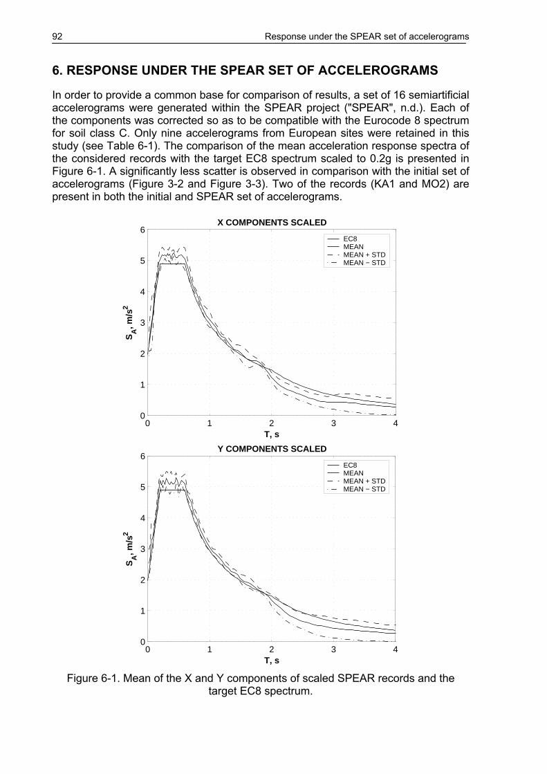
92 Response under the SPEAR set of accelerograms
6. RESPONSE UNDER THE SPEAR SET OF ACCELEROGRAMS
In order to provide a common base for comparison of results, a set of 16 semiartificial accelerograms were generated within the SPEAR project ("SPEAR", n.d.). Each of the components was corrected so as to be compatible with the Eurocode 8 spectrum for soil class C. Only nine accelerograms from European sites were retained in this study (see Table 6-1). The comparison of the mean acceleration response spectra of the considered records with the target EC8 spectrum scaled to 0.2g is presented in Figure 6-1. A significantly less scatter is observed in comparison with the initial set of accelerograms (Figure 3-2 and Figure 3-3). Two of the records (KA1 and MO2) are present in both the initial and SPEAR set of accelerograms.
0 1 2 3 40
1
2
3
4
5
6
T, s
SA
, m/s
2
X COMPONENTS SCALED
EC8MEANMEAN + STDMEAN − STD
0 1 2 3 40
1
2
3
4
5
6
T, s
SA
, m/s
2
Y COMPONENTS SCALED
EC8MEANMEAN + STDMEAN − STD
Figure 6-1. Mean of the X and Y components of scaled SPEAR records and the
target EC8 spectrum.

Response under the SPEAR set of accelerograms 93
Table 6-1. Earthquake records from the SPEAR set used in this study.
Earthquake name / Date Station name Record abbr.
Aigio 1995 OTE AIs Athens 1999 Metro ATs Duzce 1999 Bolu BOs Duzce 1999 Duzce DUs Friuli 1976 Forgario Cornino FRs Izmit 1999 Yarimca IZs Kalamata 1986 Prefecture KA1s Montenegro 1979 Hercegnovi Novi MOs Montenegro 1979 Bar-Skupstina Opstine MO2s
In this chapter the response of the SPEAR structure is assessed once again using the set of nine semiartificial accelerograms from the SPEAR set, for the sake of easier comparison with analyses performed by other researchers. It is to be noted that the same target Eurocode 8 spectrum for soil class C was used for both set of accelerograms. The main differences between the two sets of records is that the SPEAR set is much better fitted to the target spectrum, but the characteristics individual accelerograms as well as the ratio between the two components of a record are altered. Considering that the response of the SPEAR structure under the two sets of records is expected to be similar, the results are presented in less detail for the SPEAR set of accelerograms, providing however a comparison between the two suits of records. To distinguish between the two sets of results, a s suffix is added to the structural models abbreviations in the case of SPEAR suits of accelerograms (i.e. ETCPs and EFCPs). Predictions of top displacement and twist demands for the 0.2g earthquake intensity level are presented in Figure 6-2 and Figure 6-3 for the ETCPs and EFCPs models respectively. A better agreement between the dynamic and N2 predictions of top displacement demands is noted for the SPEAR set of records. It can be observed also that the torsional response is smaller under the SPEAR set of records, (smaller top storey twist and more uniform displacement demands at the flexible and stiff edges), see Figure 6-4. Interstorey drift patterns under the SPEAR suits of records are close to the ones under the initial records, but the same reduction of the torsional response is noted in the former case (see Figure 6-5). A comparison of rotation demands in beams and columns under the two accelerogram sets are presented in Figure 6-6 to Figure 6-10. Beam rotation demands are very similar for the two cases. Column rotation demands at a given storey are more uniform for the SPEAR set of records, a consequence of smaller torsional response in this case. Shear force demands in beams and columns are characterised by close values in both cases. Sample moment-rotation time-histories for beam B1 and column C2, for two of the records present in both initial and SPEAR accelerogram sets (KA1 and MO2) are presented in Figure 6-11 to Figure 6-14. Top displacement time histories for the same records may be observed in Figure 6-15 and Figure 6-16. It can be noted that the shape of the response is not changed in an important manner from the original to the semiartificial records, at least for the main peaks. For these two particular cases, the SPEAR records (KA1s and MO2s) led to an increase of the torsional response.
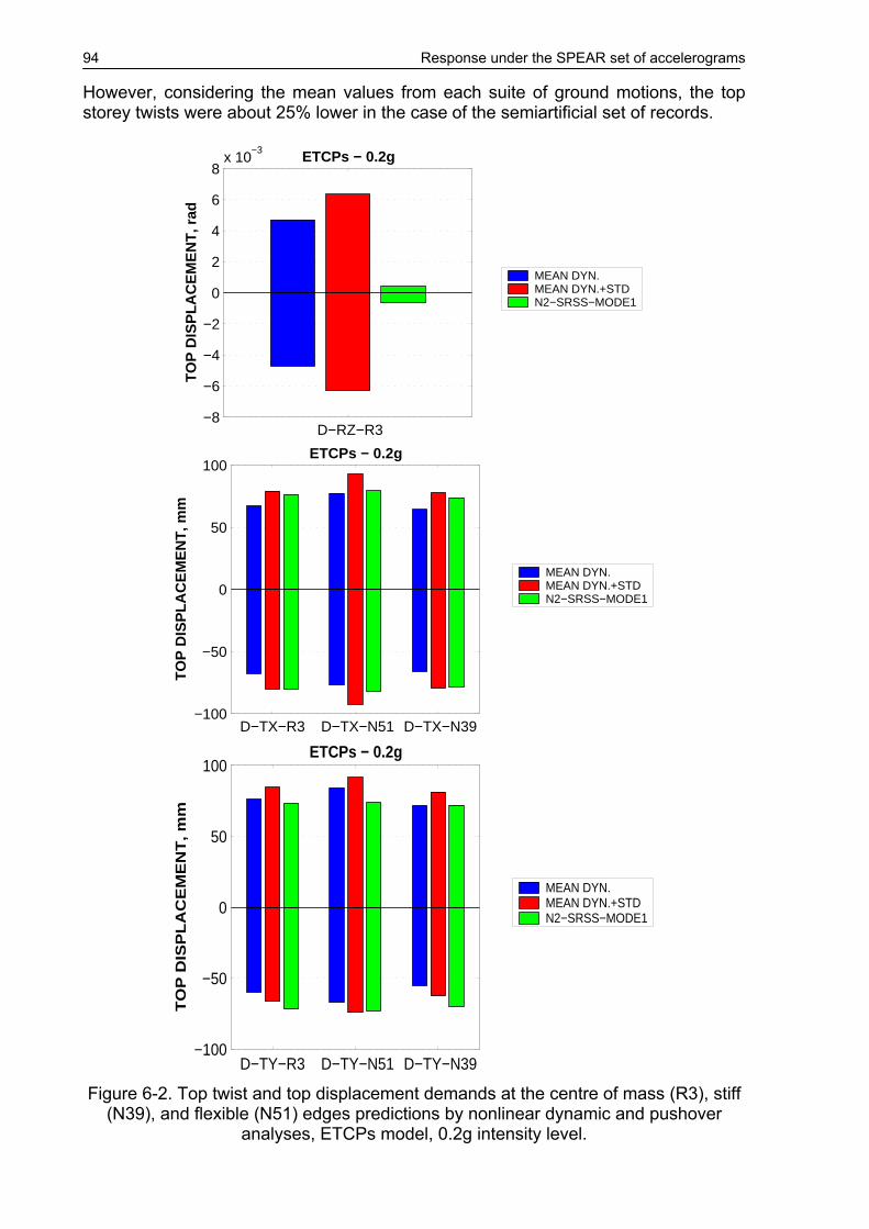
94 Response under the SPEAR set of accelerograms
However, considering the mean values from each suite of ground motions, the top storey twists were about 25% lower in the case of the semiartificial set of records.
D−RZ−R3−8
−6
−4
−2
0
2
4
6
8x 10
−3
TO
P D
ISP
LA
CE
ME
NT
, rad
ETCPs − 0.2g
MEAN DYN.MEAN DYN.+STDN2−SRSS−MODE1
D−TX−R3 D−TX−N51 D−TX−N39−100
−50
0
50
100
TO
P D
ISP
LA
CE
ME
NT
, mm
ETCPs − 0.2g
MEAN DYN.MEAN DYN.+STDN2−SRSS−MODE1
D−TY−R3 D−TY−N51 D−TY−N39−100
−50
0
50
100
TO
P D
ISP
LA
CE
ME
NT
, m
m
ETCPs − 0.2g
MEAN DYN.MEAN DYN.+STDN2−SRSS−MODE1
Figure 6-2. Top twist and top displacement demands at the centre of mass (R3), stiff
(N39), and flexible (N51) edges predictions by nonlinear dynamic and pushover analyses, ETCPs model, 0.2g intensity level.

Response under the SPEAR set of accelerograms 95
D−RZ−R3−0.01
−0.005
0
0.005
0.01
TO
P D
ISP
LA
CE
ME
NT
, rad
EFCPs − 0.2g
MEAN DYN.MEAN DYN.+STDN2−SRSS−MODE1
D−TX−R3 D−TX−N51 D−TX−N39−150
−100
−50
0
50
100
150
TO
P D
ISP
LA
CE
ME
NT
, m
m
EFCPs − 0.2g
MEAN DYN.MEAN DYN.+STDN2−SRSS−MODE1
D−TY−R3 D−TY−N51 D−TY−N39−150
−100
−50
0
50
100
150
TO
P D
ISP
LA
CE
ME
NT
, mm
EFCPs − 0.2g
MEAN DYN.MEAN DYN.+STDN2−SRSS−MODE1
Figure 6-3. Top twist and top displacement demands at the centre of mass (R3), stiff
(N39), and flexible (N51) edges predictions by nonlinear dynamic and pushover analyses, EFCPs model, 0.2g intensity level.

96 Response under the SPEAR set of accelerograms
D−RZ−R3−8
−6
−4
−2
0
2
4
6
8x 10
−3
TO
P D
ISP
LA
CE
ME
NT
, rad
0.2g
ETCPETCPs
D−TX−R3 D−TX−N51 D−TX−N39−100
−50
0
50
100
TO
P D
ISP
LA
CE
ME
NT
, mm
0.2g
ETCPETCPs
D−TY−R3 D−TY−N51 D−TY−N39−100
−50
0
50
100
TO
P D
ISP
LA
CE
ME
NT
, mm
0.2g
ETCPETCPs
Figure 6-4. Comparison of mean dynamic top displacement demands under the initial
(ETCP) and the SPEAR set of accelerograms (ETCPs).

Response under the SPEAR set of accelerograms 97
−0.015−0.01−0.005 0 0.005 0.010
2
4
6
8
10
TX, rad
HE
IGH
T, m
MEAN DYNAMIC − 0.2g − CM
ETCPETCPs
−0.01 −0.005 0 0.005 0.010
2
4
6
8
10
TY, rad
HE
IGH
T, m
MEAN DYNAMIC − 0.2g − CM
ETCPETCPs
−0.015−0.01−0.005 0 0.005 0.010
2
4
6
8
10
TX, rad
HE
IGH
T, m
MEAN DYNAMIC − 0.2g − X1Y1
ETCPETCPs
−0.01 −0.005 0 0.005 0.010
2
4
6
8
10
TY, rad
HE
IGH
T, m
MEAN DYNAMIC − 0.2g − X1Y1
ETCPETCPs
−0.015−0.01−0.005 0 0.005 0.010
2
4
6
8
10
TX, rad
HE
IGH
T, m
MEAN DYNAMIC − 0.2g − X3Y3
ETCPETCPs
−0.015−0.01−0.005 0 0.005 0.010
2
4
6
8
10
TY, rad
HE
IGH
T, m
MEAN DYNAMIC − 0.2g − X3Y3
ETCPETCPs
Figure 6-5. Comparison of interstorey drift demands for the two set of records ETCP
and ETCPs models at the centre of mass (CM), stiff (X1Y1), and flexible (X3Y3) edges.
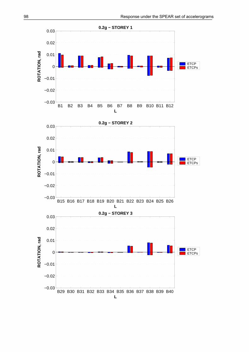
98 Response under the SPEAR set of accelerograms
B1 B2 B3 B4 B5 B6 B7 B8 B9 B10 B11 B12−0.03
−0.02
−0.01
0
0.01
0.02
0.03
L
RO
TA
TIO
N, r
ad
0.2g − STOREY 1
ETCPETCPs
B15 B16 B17 B18 B19 B20 B21 B22 B23 B24 B25 B26−0.03
−0.02
−0.01
0
0.01
0.02
0.03
L
RO
TA
TIO
N, r
ad
0.2g − STOREY 2
ETCPETCPs
B29 B30 B31 B32 B33 B34 B35 B36 B37 B38 B39 B40−0.03
−0.02
−0.01
0
0.01
0.02
0.03
L
RO
TA
TIO
N, r
ad
0.2g − STOREY 3
ETCPETCPs

Response under the SPEAR set of accelerograms 99
B1 B2 B3 B4 B5 B6 B7 B8 B9 B10 B11 B12−0.03
−0.02
−0.01
0
0.01
0.02
0.03
R
RO
TA
TIO
N, r
ad
0.2g − STOREY 1
ETCPETCPs
B15 B16 B17 B18 B19 B20 B21 B22 B23 B24 B25 B26−0.03
−0.02
−0.01
0
0.01
0.02
0.03
R
RO
TA
TIO
N, r
ad
0.2g − STOREY 2
ETCPETCPs
B29 B30 B31 B32 B33 B34 B35 B36 B37 B38 B39 B40−0.03
−0.02
−0.01
0
0.01
0.02
0.03
R
RO
TA
TIO
N, r
ad
0.2g − STOREY 3
ETCPETCPs
Figure 6-6. Rotation demands in beams, 0.2g intensity level, initial (ETCP) vs.
SPEAR (ETCPs) set of records (L – left [i] end; R – right [j] end).

100 Response under the SPEAR set of accelerograms
C1 C2 C3 C4 C5 C6 C7 C8 C90
0.005
0.01
0.015
0.02
0.025
0.03
0.035
Mx1
RO
TA
TIO
N, r
ad
0.2g − STOREY 1
ETCPETCPs
C10 C11 C12 C13 C14 C15 C16 C17 C180
0.005
0.01
0.015
0.02
0.025
0.03
0.035
Mx1
RO
TA
TIO
N, r
ad
0.2g − STOREY 2
ETCPETCPs
C19 C20 C21 C22 C23 C24 C25 C26 C270
0.005
0.01
0.015
0.02
0.025
0.03
0.035
Mx1
RO
TA
TIO
N, r
ad
0.2g − STOREY 3
ETCPETCPs
Figure 6-7. Rotation demands in columns (bending about X axis at the bottom end),
0.2g intensity level, initial (ETCP) vs. SPEAR (ETCPs) set of records.
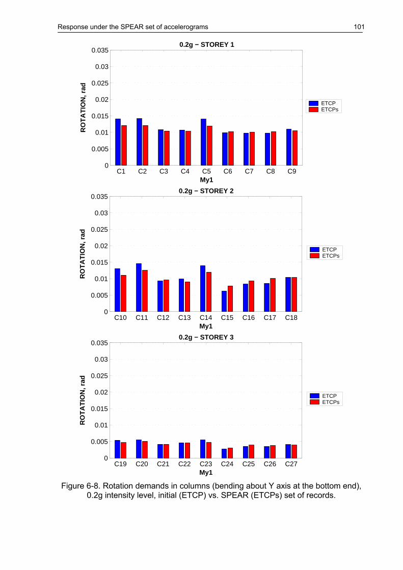
Response under the SPEAR set of accelerograms 101
C1 C2 C3 C4 C5 C6 C7 C8 C90
0.005
0.01
0.015
0.02
0.025
0.03
0.035
My1
RO
TA
TIO
N, r
ad
0.2g − STOREY 1
ETCPETCPs
C10 C11 C12 C13 C14 C15 C16 C17 C180
0.005
0.01
0.015
0.02
0.025
0.03
0.035
My1
RO
TA
TIO
N, r
ad
0.2g − STOREY 2
ETCPETCPs
C19 C20 C21 C22 C23 C24 C25 C26 C270
0.005
0.01
0.015
0.02
0.025
0.03
0.035
My1
RO
TA
TIO
N, r
ad
0.2g − STOREY 3
ETCPETCPs
Figure 6-8. Rotation demands in columns (bending about Y axis at the bottom end),
0.2g intensity level, initial (ETCP) vs. SPEAR (ETCPs) set of records.
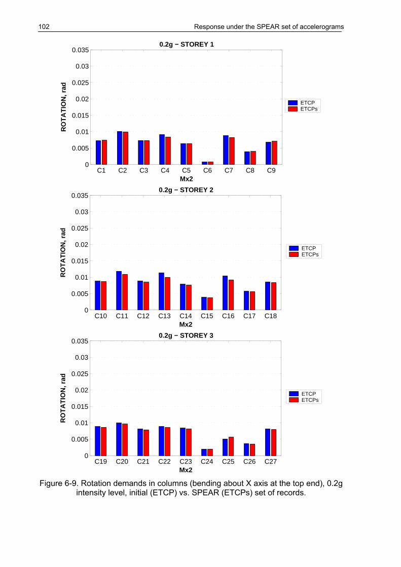
102 Response under the SPEAR set of accelerograms
C1 C2 C3 C4 C5 C6 C7 C8 C90
0.005
0.01
0.015
0.02
0.025
0.03
0.035
Mx2
RO
TA
TIO
N, r
ad
0.2g − STOREY 1
ETCPETCPs
C10 C11 C12 C13 C14 C15 C16 C17 C180
0.005
0.01
0.015
0.02
0.025
0.03
0.035
Mx2
RO
TA
TIO
N, r
ad
0.2g − STOREY 2
ETCPETCPs
C19 C20 C21 C22 C23 C24 C25 C26 C270
0.005
0.01
0.015
0.02
0.025
0.03
0.035
Mx2
RO
TA
TIO
N, r
ad
0.2g − STOREY 3
ETCPETCPs
Figure 6-9. Rotation demands in columns (bending about X axis at the top end), 0.2g
intensity level, initial (ETCP) vs. SPEAR (ETCPs) set of records.

Response under the SPEAR set of accelerograms 103
C1 C2 C3 C4 C5 C6 C7 C8 C90
0.005
0.01
0.015
0.02
0.025
0.03
0.035
My2
RO
TA
TIO
N, r
ad
0.2g − STOREY 1
ETCPETCPs
C10 C11 C12 C13 C14 C15 C16 C17 C180
0.005
0.01
0.015
0.02
0.025
0.03
0.035
My2
RO
TA
TIO
N, r
ad
0.2g − STOREY 2
ETCPETCPs
C19 C20 C21 C22 C23 C24 C25 C26 C270
0.005
0.01
0.015
0.02
0.025
0.03
0.035
My2
RO
TA
TIO
N, r
ad
0.2g − STOREY 3
ETCPETCPs
Figure 6-10. Rotation demands in columns (bending about Y axis at the top end),
0.2g intensity level, initial (ETCP) vs. SPEAR (ETCPs) set of records.

104 Response under the SPEAR set of accelerograms
−0.02 −0.01 0 0.01 0.02−60
−40
−20
0
20
40
60
L − ROTATION, rad
MO
ME
NT
, kN
mETCP − 0.2g − B1 − KA1−0
−0.02 −0.01 0 0.01 0.02−60
−40
−20
0
20
40
60
L − ROTATION, rad
MO
ME
NT
, kN
m
ETCPs − 0.2g − B1 − KA1s−0
Figure 6-11. Comparison of moment-rotation history for the beam B1 left end (i),
ETCP model, under initial (KA1-0) and SPEAR (KA1s-0) records.
−0.02 −0.01 0 0.01 0.02−60
−40
−20
0
20
40
60
L − ROTATION, rad
MO
ME
NT
, kN
m
ETCP − 0.2g − B1 − MO2−0
−0.02 −0.01 0 0.01 0.02−60
−40
−20
0
20
40
60
L − ROTATION, rad
MO
ME
NT
, kN
mETCPs − 0.2g − B1 − MO2s−0
Figure 6-12. Comparison of moment-rotation history for the beam B1 left end (i),
EFCP model, under initial (KA1-0) and SPEAR (KA1s-0) records.
−0.02 −0.01 0 0.01 0.02
−60
−40
−20
0
20
40
60
Mx1 − ROTATION, rad
MO
ME
NT
, kN
m
ETCP − 0.2g − C2 − KA1−0
−0.02 −0.01 0 0.01 0.02
−60
−40
−20
0
20
40
60
Mx1 − ROTATION, rad
MO
ME
NT
, kN
m
ETCPs − 0.2g − C2 − KA1s−0

Response under the SPEAR set of accelerograms 105
−0.02 −0.01 0 0.01 0.02
−60
−40
−20
0
20
40
60
My1 − ROTATION, rad
MO
ME
NT
, kN
m
ETCP − 0.2g − C2 − KA1−0
−0.02 −0.01 0 0.01 0.02
−60
−40
−20
0
20
40
60
My1 − ROTATION, rad
MO
ME
NT
, kN
m
ETCPs − 0.2g − C2 − KA1s−0
Figure 6-13. Comparison of moment-rotation history for the column C2 bottom end,
ETCP model, under initial (KA1-0) and SPEAR (KA1s-0) records.
−0.06 −0.04 −0.02 0 0.02 0.04
−60
−40
−20
0
20
40
60
Mx1 − CURVATURE, 1/m
MO
ME
NT
, kN
m
EFCP − 0.2g − C2 − KA1−0
−0.06 −0.04 −0.02 0 0.02 0.04
−60
−40
−20
0
20
40
60
Mx1 − CURVATURE, 1/m
MO
ME
NT
, kN
m
EFCPs − 0.2g − C2 − KA1s−0
−0.06 −0.04 −0.02 0 0.02 0.04
−60
−40
−20
0
20
40
60
My1 − CURVATURE, 1/m
MO
ME
NT
, kN
m
EFCP − 0.2g − C2 − KA1−0
−0.06 −0.04 −0.02 0 0.02 0.04
−60
−40
−20
0
20
40
60
My1 − CURVATURE, 1/m
MO
ME
NT
, kN
m
EFCPs − 0.2g − C2 − KA1s−0
Figure 6-14. Comparison of moment-rotation history for the column C2 bottom end,
EFCP model, under initial (KA1-0) and SPEAR (KA1s-0) records.

106 Response under the SPEAR set of accelerograms
0 2 4 6 8 10 12 14 16 18 20 22−100
−50
0
50
100
TIME, s
DIS
PL
AC
EM
EN
T, m
m
ETCP − 0.2g − TOP DISPLACEMENT TH, KA1−0
D−TX−N39 D−TX−N51
0 2 4 6 8 10 12 14 16 18 20 22−5
0
5
RO
TA
TIO
N, m
rad
D−RZ−R3
0 2 4 6 8 10 12 14 16 18 20 22−100
−50
0
50
100
TIME, s
DIS
PL
AC
EM
EN
T, m
m
ETCPs − 0.2g − TOP DISPLACEMENT TH, KA1s−0
D−TX−N39 D−TX−N51
0 2 4 6 8 10 12 14 16 18 20 22−5
0
5
RO
TA
TIO
N, m
rad
D−RZ−R3
Figure 6-15. Time histories of top twist and top displacements in the X direction,
ETCP model, under initial (KA1-0) and SPEAR (KA1s-0) records.
0 2 4 6 8 10 12 14 16 18 20 22−200
−100
0
100
200
TIME, s
DIS
PL
AC
EM
EN
T, m
m
ETCP − 0.2g − TOP DISPLACEMENT TH, MO2−0
D−TX−N39 D−TX−N51
0 2 4 6 8 10 12 14 16 18 20 22−10
−5
0
5
10
RO
TA
TIO
N, m
rad
D−RZ−R3
0 2 4 6 8 10 12 14 16 18 20 22−200
−100
0
100
200
TIME, s
DIS
PL
AC
EM
EN
T, m
m
ETCPs − 0.2g − TOP DISPLACEMENT TH, MO2s−0
D−TX−N39 D−TX−N51
0 2 4 6 8 10 12 14 16 18 20 22−10
−5
0
5
10
RO
TA
TIO
N, m
rad
D−RZ−R3
Figure 6-16. Time histories of top twist and top displacements in the X direction,
ETCP model, under initial (MO2-0) and SPEAR (MO2s-0) records.

Summary and Conclusions 107
7. SUMMARY AND CONCLUSIONS
This report describes the assessment of seismic response of a gravity load designed r.c. building to be tested pseudo-dynamically at ELSA in Ispra, within the EU project Seismic Performance Assessment and Rehabilitation (SPEAR). The main deficiencies of the SPEAR test structure are: use of plain reinforcing bars slender columns (250x250), with largely spaced stirrups inclined reinforcement in beams for shear resistance and optimal distribution of
reinforcement column lap splices in potential plastic hinge zones lack of shear reinforcement in beam-column joints inadequate anchorage of stirrups (90° hooks) irregular plan layout (torsionally unbalanced)
Two 3D structural models were used, one based on one-component concentrated plasticity elements, and another one that used distributed plasticity fibre elements for columns. While the latter model is believed to estimate better the structural response in the inelastic range, the former model has the advantage of easier interpretation of results, evaluation of seismic capacity being on the safe side in comparison to the more complex fibre model. For each of the models, seismic demand was evaluated by the N2 method and by inelastic dynamic analysis. Two sets of earthquake records were used. The first one is a suite of seven recorded bidirectional ground motions, scaled to match the EC8 spectra for soil type C in the constant velocity range. A second suite of semiartificial earthquake records provided within the SPEAR project were added later to provide easier comparison of results with other project tasks. Seismic performance of the SPEAR structure was assessed for three earthquake intensity levels: 0.1g, 0.2g, and 0.3g. The structure is torsionally unbalanced, with eccentricities higher in the Y direction. Due to the strong 250x750 column resisting horizontal loading in the Y direction, base shear capacity is higher in the Y direction. At the same time, the structure is characterised by unsymmetrical strength and stiffness in the positive and negative Y direction. As a consequence, displacement demands are higher in the weaker X direction, and are different in the positive and negative Y direction. The latter phenomenon observed for time-history analysis, is not represented well by the pushover analysis. Average increase of top displacements (mean dynamic) at the flexible edge with respect to the centre of mass amounts to 30% and 16% for the X and Y direction respectively. Corresponding decrease of top displacements at the stiff edge with respect to centre of mass amounts to 15% and 10% for X and Y directions respectively. Thus a higher torsional response is present in the X direction, even if the initial elastic eccentricity is bigger in the Y direction. Interstorey drift demands concentrate in the lower two storeys, but are more uniform in the Y direction. Damage to the SPEAR structure is dictated by weak columns (with the exception of the 250x750 C6-20-30 column) and by significantly lower moment capacity under positive bending for beams. Pullout of bottom beam reinforcement and extensive concrete spalling are dominant failure modes. Though there is a lack of proper transverse reinforcement both in elements and in beam-column joints, shear capacity checks indicate that neither elements nor joints are susceptible to shear failures. Damage to beams is more important for shorter elements and at the exterior joints, due to higher potential for moment reversals. Column demand to capacity ratios are

108 Summary and Conclusions
higher for columns at the flexible edges (higher demands) and for elements with higher axial loads (lower rotation capacities). Column DCRs are higher for bending about the Y axis, due to higher displacement demands in the X direction. The critical column is the first storey central column (C3). Another three columns from the first storey (C1, C2, and C4) follow closely with slightly lower DCRs. Pullout of bottom beam reinforcement and yielding of columns is expected already at 0.1g intensity level, but without concrete spalling. Significantly higher damage, including extensive cover concrete spalling for the C1-C4 columns is predicted at the 0.2g intensity level. Initiation of significant global structural damage is evaluated to 0.24g by dynamic analysis, and 0.22g by the N2 method. However, the distributed plasticity fibre model indicated that the structure may retain its load-bearing capacity up to higher intensities (0.3g). This may change however, for more unfavourable ratio of steel to concrete strength, an increase of steel strength in comparison with the concrete strength leading to more pronounced strength degradation of columns. Though a similar response was obtained for both suites of earthquake records, torsional response was significantly lower in the case of the semiartificial records. Thus, top storey twists were about 25% lower in the case of the SPEAR set of records.

Summary and Conclusions 109
ACKNOWLEDGEMENTS
The work presented in this report was performed by Aurel Stratan under the supervision of Peter Fajfar. Aurel Stratan is a Ph.D. student at the Politehnica University of Timisoara, Romania, who spent ten and a half months as a visiting researcher at the University of Ljubljana, Slovenia, within the SAFERR research training network funded by the European Comission (Safety Assessment for Seismic Risk Reduction, HPRN-CT-1999-00035). The work is related to the SPEAR project (Seismic Performance Assessment and Rehabilitation, G6RD-CT-2001-00525).

110 Summary and Conclusions
REFERENCES
Ambraseys, N., Smit, P., Berardi, R., Rinaldis, D., Cotton, F., and Berge-Thierry, C., (2000) "Dissemination of European Strong-Motion Data", CD-ROM Collection. European Council, Environment and Climate Research Programme. Aycardi, L., Mander, J.B., Reinhorn, A.M., (1994) "Seismic Resistance of Reinforced Concrete Frame Structures Designed Only for Gravity Loads: Experimental Performance of Subassemblages", ACI Structural Journal, V.91, No.5, 552-563. Calvi, G.M., Magenes, G., and Pampanin, S., (2002) "Relevance of Beam-Column Joint Damage and Collapse in RC Frame Assessment", Journal of Earthquake Engineering, Vol. 6, special issue No.1, 75-100. Cosenza, E., Manfredi, G., and Verderame, G.M., (2002) "Seismic Assessment of Gravity Load Designed R.C. Frames: Critical Issues in Structural Modelling", Journal of Earthquake Engineering, Vol. 6, special issue No.1, 101-122 Eurocode 2, (2001) "Design of concrete structures", European Committee for Standardisation (CEN), final draft. Eurocode 8, (2002) "Design provisions for earthquake resistance of structures", European Committee for Standardisation (CEN), Draft No.5. Fajfar, P., (2000). "A nonlinear analysis method for performance-based seismic design". Earthquake Spectra 2000, 16(3): 573-92. Fajfar, P., (2002). "Extension of the N2 method to asymmetric buildings – theoretical background". Proc. of Slovenia – Japan Workshops on Performance Based Seismic Design Methodologies, Ljubljana, Slovenia, March 2002. Fardis, M.N, (2002) "Design of an Irregular Building for the SPEAR Project". FEMA 356, (2000) "Prestandard and commentary for the seismic rehabilitation of buildings", Federal Emergency Management Agency, Washington (DC). Hakuto, S., Park, R., and Tanaka, H., (2000) "Seismic Load Tests on Interior and Exterior Beam-Column Joints with Substandard Reinforcing Details", ACI Structural Journal, V.97, No.1, 11-25. Kunnath, K., Hoffman, G., Reinhorn, A.M, and Mander, B., (1995) "Gravity-Load-Designed Reinforced Concrete Buildings – Part I: Seismic Evaluation of Existing Construction", ACI Structural Journal, V.92, No.3, 343-354. Li, K., (2002) "CANNY 99: 3-Dimensional nonlinear static/dynamic structural analysis computer program". Technical manual and User manual. Park, R., (2002) "A Summary of Results of Simulated Seismic Load Tests on Reinforced Concrete Beam-Column Joints, Beams and Columns with Substandard Reinforcing Details", Journal of Earthquake Engineering, Vol. 6, No.2, 147-174 Paulay, T. and Priestley, M.J.N., (1992) "Seismic Design of Reinforced Concrete and Masonry Buildings", John Wiley & Sons, Inc., New York. Penelis G.G. and Kappos A.J. (1997). "Earthquake-Resistant Concrete Structures". E&FN SPON. Priestley, M.J.N., Verma, R., and Xiao, Y., (1994) "Seismic Shear Strength Demand of Reinforced Concrete Columns", Journal of Structural Engineering, Vol. 120, No.8, 2310-2329.

Summary and Conclusions 111
Priestley, M.J.N., (1997) "Displacement-Based Seismic Assessment of Reinforced Concrete Buildings", Journal of Earthquake Engineering, Vol. 1, No.1, 157-192. SPEAR web site (n.d.) retrieved on 10/07/2002 from http://www.strulab.civil.upatras.gr/spear Stratan, A., and Fajfar, P., (2002) "Influence of modelling assumptions and analysis procedure on the seismic evaluation of reinforced concrete GLD frames". IKPIR Report, University of Ljubljana.

112 Description of the SPEAR structure
ANNEX I. Description of the SPEAR structure
UNIVERSITY OF PATRASSTRUCTURES LABORATORY
1
Description of the 3-storey structure
The structure is a simplification of an actual 3-storey building representative of older construction in Greece, without engineered earthquake resistance. It has been designed for gravity loads alone, using the concrete design code applying in Greece between 1954 and 1995, with the construction practice and materials used in Greece in the early 70’s. The structural configuration is also typical of non-earthquake-resistant construction of that period.
The storey height is 3.0m, from top to top of the slab (net storey height 2.50m under beams). The plan of the framing and the cross-sectional dimensions of members (in cms) are given in the preceding drawings. The slab thickness is 150mm.
At present time the concrete can be considered to have fc=25MPa. The reinforcement consists of smooth bars and assumed to have as fy the nominal yield strength (320MPa).
Design gravity loads on slabs are 0.5kN/m2 for finishings and 2kN/m2 for live loads.
The reinforcement of the various structural elements is given below.
Slabs: 8mm bars at 200mm centres, both ways (or equivalent welded wire mesh)
Beam Longitudinal Reinforcement Top bars (“montage”): Two 12mm diameter bars, anchored with 180° hook at far end of column,
w/o downward bent. Bottom bars:
1. Two bars (three in Beam 4) continue straight to the supports, where they are anchored w/
180° hook at far end of column. 2. Two (or 3 in Beam 7 or 4 in Beam 4) bars are bent up towards the supports, at locations
indicated in the drawings; their bent-up ends are bent down at the far end of exterior
columns and anchored w/ 180° hook at the level of the beam soffit; over interior columns
they continue straight into next span, anchored at the top flange w/ 180° hook as indicated in the drawings.
Added top bars in Beams 9 and 10 over support at column C3: Two 20mm diameter bars are
added at top over C3, bent-down at 45° towards the span very close to the face of C3 and
anchored at beam bottom w/ 180° hooks as indicated in the drawings.
Beam stirrups8mm diameter bars at 200mm centers, closed at top w/ 90° hooks, as indicated in the drawings.
Stirrups do not continue in the joints.
Column Vertical Reinforcement and Stirrups 1. 12mm bars, as indicated in the drawings, within 8mm diameter stirrups at 250mm centers,
closed w 90° hooks. 2. Clear cover of stirrups: 15mm 3. Stirrups do not continue in the joints. 4. Vertical bars are lap spliced over 400mm at floor level, including the 1st storey (w/ starter
bars); spliced bars have 180° hooks.

Description of the SPEAR structure 113
UNIVERSITY OF PATRASSTRUCTURES LABORATORY
2
3.0 5.0
5.5
5.0
6.0
4.0
1.0
1.70
COLUMNS C1-C5 & C7-C9
0,2
5
0,25
STIRRUPS �8/25
4�12 10�12
STIRRUPS �8/25
COLUMN C6
0,25
0,7
5
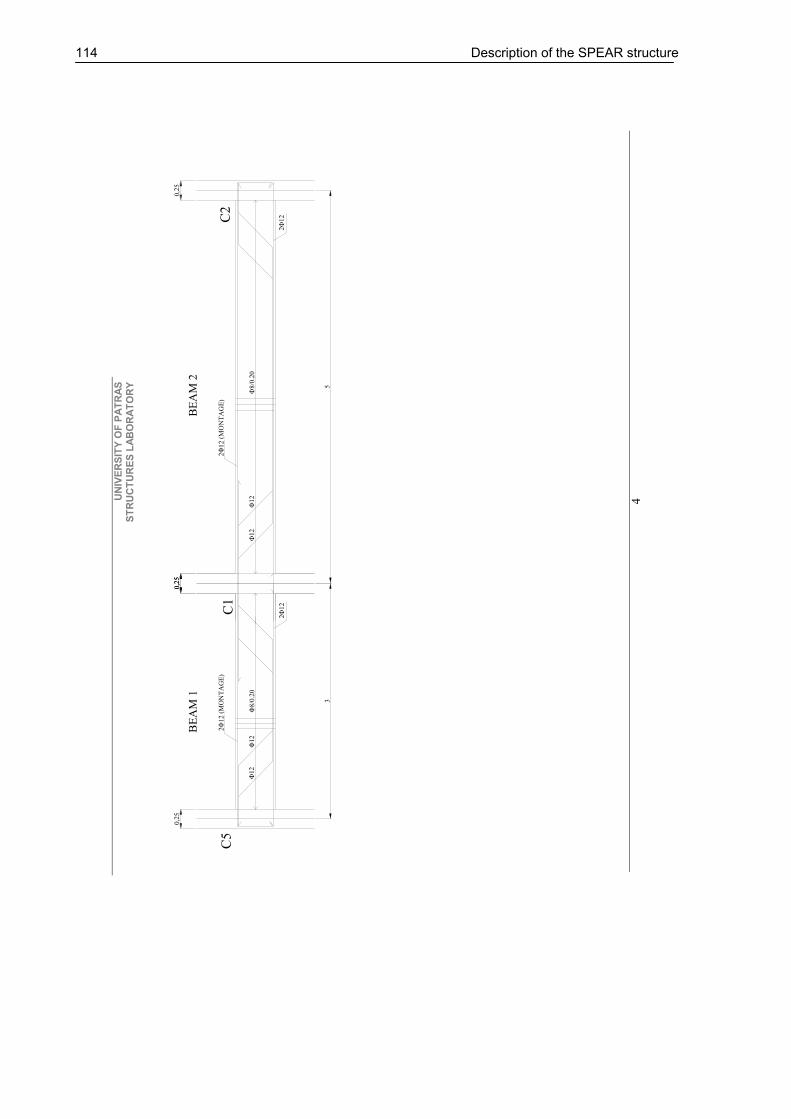
114 Description of the SPEAR structure
UN
IVER
SITY
OF
PATR
ASST
RU
CTU
RES
LAB
OR
ATO
RY
4
BE
AM
1
0,2
50
,25
3
C5
C1
2�
12 (
MO
NT
AG
E)
2�
12
�8
/0.2
0
5
0,2
5
�8/0
.20
2�
12 (
MO
NT
AG
E)
2�
12C2
0,2
5
BE
AM
2
�12
�12
�12
�12

Description of the SPEAR structure 115
UN
IVER
SITY
OF
PATR
ASST
RU
CTU
RES
LAB
OR
ATO
RY
5
3
BE
AM
3
2�
12
(M
ON
TA
GE
)9
0,2
5
2�
12
0,2
5
�8/0
.20
�12
�12
BE
AM
9

116 Description of the SPEAR structure
UN
IVER
SITY
OF
PATR
ASST
RU
CTU
RES
LAB
OR
ATO
RY
6
6
0,2
5
BE
AM
4
0,2
5
3C
4
3�
20
2�
12
(MO
NT
AG
E)
�8
/0.2
0�
8/0
.20
�20
�20
�20
�20
BE
AM
7
BE
AM
5
3
0,2
50
,25
C8
C6
2�
12
(M
ON
TA
GE
)
2�
12
�8
/0.2
0�
12
�12
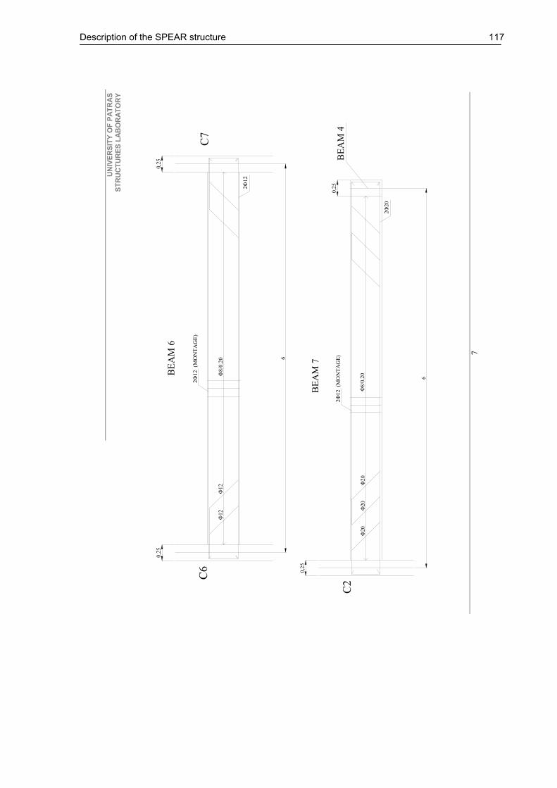
Description of the SPEAR structure 117
UN
IVER
SITY
OF
PATR
AS
STR
UC
TUR
ES L
ABO
RAT
OR
Y
7
6
0,2
5
BE
AM
6
0,2
5
C6
C7
2�
12
2�
12
(MO
NT
AG
E)
�8/0
.20
�12
�1
2
6
0,2
5
BE
AM
7
0,2
5
C2
2�
20
2�
12
(M
ON
TA
GE
)
�8
/0.2
0�
20
�2
0�
20
BE
AM
4
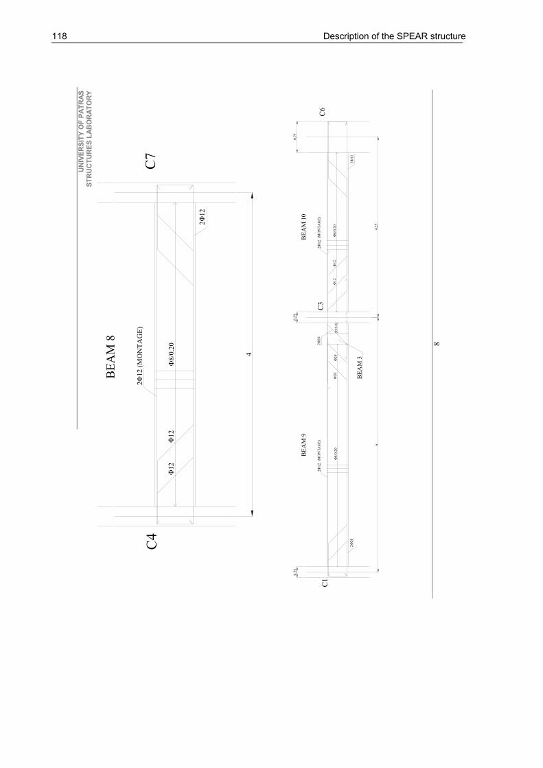
118 Description of the SPEAR structure
UN
IVER
SITY
OF
PATR
AS
STR
UC
TUR
ES L
ABO
RAT
OR
Y
8
4
BE
AM
8
C4
C7
2�
12
2�
12 (
MO
NT
AG
E)
�8
/0.2
0�
12
�12
6
0,2
50
,25
BE
AM
9
C1
2�
20
2�
12
(M
ON
TA
GE
)
�8/0
.20
�8/0
.20
2�
20
4,2
5
�8
/0.2
0
2�
12
0,7
5
2�
12
(M
ON
TA
GE
)C
3
BE
AM
10
C6
�20
�20
�1
2�
12
BE
AM
3
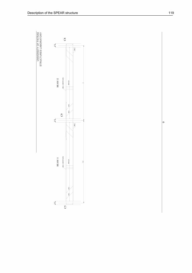
Description of the SPEAR structure 119
UN
IVER
SITY
OF
PATR
AS
STR
UC
TUR
ES L
ABO
RAT
OR
Y
9
BE
AM
11
5,5
0,2
50,2
5
C5
C9
2�
12
2�
12
(M
ON
TA
GE
)
�8
/0.2
0
5
�8/0
.20
2�
12
(MO
NT
AG
E)
2�
12
0,2
5
BE
AM
12
C8
�12
�1
2�
12
�1
2

120 Description of the SPEAR structure
UN
IVER
SITY
OF
PATR
AS
STR
UC
TUR
ES L
ABO
RAT
OR
Y
10
S1
15
S2
15
S5
15
S3
15
S4
15
�8
/20
�8
/10
�8/4
0
�8/40
�8/20
�8/20
�8/40
�8
/20
�8/40
�8/40
�8
/40
�8
/20
�8/2
0
�8/40

Acceleration time-histories and response spectra of considered ground motions 121
ANNEX II. Acceleration time-histories and response spectra of considered ground motions
0 1 2 3 40
5
10
15
T, s
SA
, m/s
2
SRSS OF UNSCALED RECORDS
Alkion Korinthos−OTEBuilding Alkion Xilokastro−OTEBuilding CampanoLucano Calitri Kalamata Kalamata−Prefecture Kalamata Kalamata−OTEBuilding Montenegro Ulcinj−HotelAlbatros Montenegro Bar−SkupstinaOpstineMEANEC8
Figure A - 1. Square Root of Sum of Squares (SRSS) spectra of unscaled records.
0 1 2 3 40
5
10
15
T, s
SA
, m/s
2
SRSS OF SCALED RECORDS
Alkion Korinthos−OTEBuilding Alkion Xilokastro−OTEBuilding CampanoLucano Calitri Kalamata Kalamata−Prefecture Kalamata Kalamata−OTEBuilding Montenegro Ulcinj−HotelAlbatros Montenegro Bar−SkupstinaOpstineMEANEC8
Figure A - 2. Square Root of Sum of Squares (SRSS) spectra of scaled records.

122 Acceleration time-histories and response spectra of considered ground motions
0 1 2 3 40
2
4
6
8
10
T, s
SA
, m/s
2
X COMPONENTS SCALED
Alkion Korinthos−OTEBuilding Alkion Xilokastro−OTEBuilding CampanoLucano Calitri Kalamata Kalamata−Prefecture Kalamata Kalamata−OTEBuilding Montenegro Ulcinj−HotelAlbatros Montenegro Bar−SkupstinaOpstineMEANEC8
Figure A - 3. Acceleration response spectra of scaled records (X components).
0 1 2 3 40
2
4
6
8
10
12
14
T, s
SA
, m/s
2
Y COMPONENTS SCALED
Alkion Korinthos−OTEBuilding Alkion Xilokastro−OTEBuilding CampanoLucano Calitri Kalamata Kalamata−Prefecture Kalamata Kalamata−OTEBuilding Montenegro Ulcinj−HotelAlbatros Montenegro Bar−SkupstinaOpstineMEANEC8
Figure A - 4. Acceleration response spectra of scaled records (Y components).

Acceleration time-histories and response spectra of considered ground motions 123
0 5 10 15 20 25 30 35 40 45−4
−2
0
2
4
2.42
−2.17
TIME, s
X C
OM
PO
NE
NT
, m/s
2
ACCELERATION TIME HISTORY − Alkion Korinthos−OTEBuilding (AL1 )
maxmin
0 5 10 15 20 25 30 35 40 45−4
−2
0
2
43.26
−2.4
TIME, s
Y C
OM
PO
NE
NT
, m/s
2
ACCELERATION TIME HISTORY − Alkion Korinthos−OTEBuilding (AL1 )
maxmin
0 5 10 15 20 25 30 35 40−4
−2
0
2
4
2.43
−2.66
TIME, s
X C
OM
PO
NE
NT
, m/s
2
ACCELERATION TIME HISTORY − Alkion Xilokastro−OTEBuilding (AL2 )
maxmin
0 5 10 15 20 25 30 35 40−4
−2
0
2
4
1.57
−1.25
TIME, s
Y C
OM
PO
NE
NT
, m/s
2
ACCELERATION TIME HISTORY − Alkion Xilokastro−OTEBuilding (AL2 )
maxmin

124 Acceleration time-histories and response spectra of considered ground motions
0 10 20 30 40 50 60 70 80 90−4
−2
0
2
4
1.06
−1.24
TIME, s
X C
OM
PO
NE
NT
, m/s
2ACCELERATION TIME HISTORY − CampanoLucano Calitri (CA1 )
maxmin
0 10 20 30 40 50 60 70 80 90−4
−2
0
2
4
1.13
−1.4
TIME, s
Y C
OM
PO
NE
NT
, m/s
2
ACCELERATION TIME HISTORY − CampanoLucano Calitri (CA1 )
maxmin
0 5 10 15 20 25 30−4
−2
0
2
4
1.66
−1.67
TIME, s
X C
OM
PO
NE
NT
, m/s
2
ACCELERATION TIME HISTORY − Kalamata Kalamata−Prefecture (KA1 )
maxmin
0 5 10 15 20 25 30−4
−2
0
2
4
1.82
−2.3
TIME, s
Y C
OM
PO
NE
NT
, m/s
2
ACCELERATION TIME HISTORY − Kalamata Kalamata−Prefecture (KA1 )
maxmin
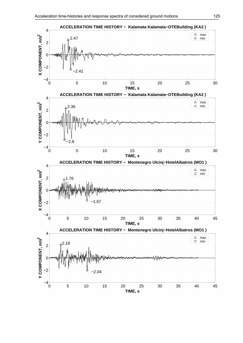
Acceleration time-histories and response spectra of considered ground motions 125
0 5 10 15 20 25 30−4
−2
0
2
4
2.47
−2.41
TIME, s
X C
OM
PO
NE
NT
, m/s
2
ACCELERATION TIME HISTORY − Kalamata Kalamata−OTEBuilding (KA2 )
maxmin
0 5 10 15 20 25 30−4
−2
0
2
4
2.36
−2.8
TIME, s
Y C
OM
PO
NE
NT
, m/s
2
ACCELERATION TIME HISTORY − Kalamata Kalamata−OTEBuilding (KA2 )
maxmin
0 5 10 15 20 25 30 35 40 45−4
−2
0
2
4
1.76
−1.67
TIME, s
X C
OM
PO
NE
NT
, m/s
2
ACCELERATION TIME HISTORY − Montenegro Ulcinj−HotelAlbatros (MO1 )
maxmin
0 5 10 15 20 25 30 35 40 45−4
−2
0
2
4
2.18
−2.04
TIME, s
Y C
OM
PO
NE
NT
, m/s
2
ACCELERATION TIME HISTORY − Montenegro Ulcinj−HotelAlbatros (MO1 )
maxmin

126 Acceleration time-histories and response spectra of considered ground motions
0 5 10 15 20 25 30 35 40 45 50−4
−2
0
2
4
1.43
−1.15
TIME, s
X C
OM
PO
NE
NT
, m/s
2ACCELERATION TIME HISTORY − Montenegro Bar−SkupstinaOpstine (MO2 )
maxmin
0 5 10 15 20 25 30 35 40 45 50−4
−2
0
2
4
1.34
−1.38
TIME, s
Y C
OM
PO
NE
NT
, m/s
2
ACCELERATION TIME HISTORY − Montenegro Bar−SkupstinaOpstine (MO2 )
maxmin
Figure A - 5. Acceleration time-histories of horizontal components of scaled ground
motions.

Moment-curvature and moment–rotation idealisation of elements for one-component model 127
ANNEX III. Moment-curvature and moment–rotation idealisation of elements for one-component model
0 0.05 0.1 0.150
20
40
60
80
100
CURVATURE, 1/m
MO
ME
NT
, kN
m
B1I, B5IJ−POSB1I, B5IJ−NEG
0 0.005 0.01 0.015 0.02 0.0250
20
40
60
80
100
ROTATION, rad
MO
ME
NT
, kN
m
B1I, B5IJ−POSB1I, B5IJ−NEG
0 0.05 0.1 0.150
50
100
150
200
CURVATURE, 1/m
MO
ME
NT
, kN
m
B1J−POSB1J−NEG
0 0.005 0.01 0.015 0.02 0.0250
50
100
150
200
ROTATION, rad
MO
ME
NT
, kN
m
B1J−POSB1J−NEG
0 0.05 0.1 0.150
50
100
150
200
250
CURVATURE, 1/m
MO
ME
NT
, kN
m
B2I−POSB2I−NEG
0 0.01 0.02 0.030
50
100
150
200
250
ROTATION, rad
MO
ME
NT
, kN
m
B2I−POSB2I−NEG
0 0.05 0.1 0.150
50
100
150
200
CURVATURE, 1/m
MO
ME
NT
, kN
m
B2J−POSB2J−NEG
0 0.01 0.02 0.030
50
100
150
200
ROTATION, rad
MO
ME
NT
, kN
m
B2J−POSB2J−NEG
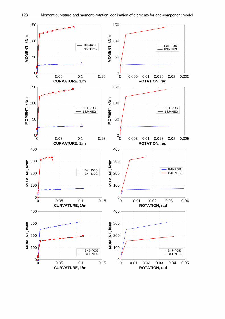
128 Moment-curvature and moment–rotation idealisation of elements for one-component model
0 0.05 0.1 0.150
50
100
150
CURVATURE, 1/m
MO
ME
NT
, kN
m
B3I−POSB3I−NEG
0 0.005 0.01 0.015 0.02 0.0250
50
100
150
ROTATION, rad
MO
ME
NT
, kN
m
B3I−POSB3I−NEG
0 0.05 0.1 0.150
50
100
150
CURVATURE, 1/m
MO
ME
NT
, kN
m
B3J−POSB3J−NEG
0 0.005 0.01 0.015 0.02 0.0250
50
100
150
ROTATION, rad
MO
ME
NT
, kN
mB3J−POSB3J−NEG
0 0.05 0.1 0.150
100
200
300
400
CURVATURE, 1/m
MO
ME
NT
, kN
m
B4I−POSB4I−NEG
0 0.01 0.02 0.03 0.040
100
200
300
400
ROTATION, rad
MO
ME
NT
, kN
m
B4I−POSB4I−NEG
0 0.05 0.1 0.150
100
200
300
400
CURVATURE, 1/m
MO
ME
NT
, kN
m
B4J−POSB4J−NEG
0 0.01 0.02 0.03 0.04 0.050
100
200
300
400
ROTATION, rad
MO
ME
NT
, kN
m
B4J−POSB4J−NEG
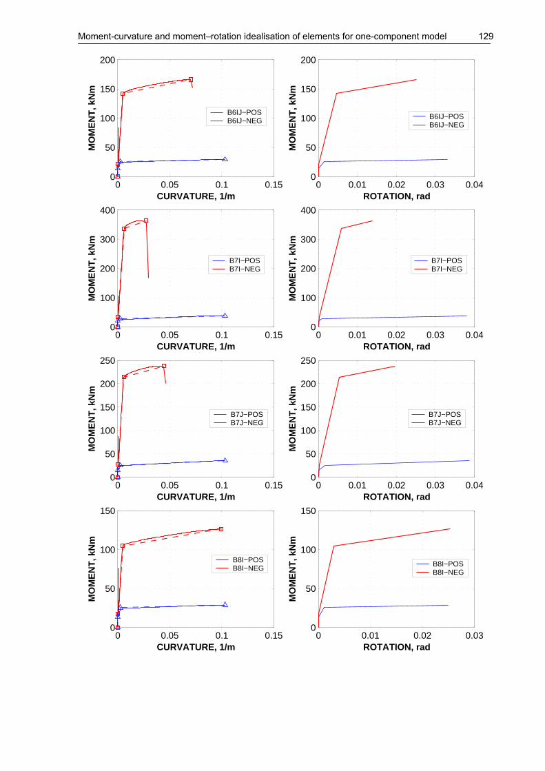
Moment-curvature and moment–rotation idealisation of elements for one-component model 129
0 0.05 0.1 0.150
50
100
150
200
CURVATURE, 1/m
MO
ME
NT
, kN
m
B6IJ−POSB6IJ−NEG
0 0.01 0.02 0.03 0.040
50
100
150
200
ROTATION, rad
MO
ME
NT
, kN
m
B6IJ−POSB6IJ−NEG
0 0.05 0.1 0.150
100
200
300
400
CURVATURE, 1/m
MO
ME
NT
, kN
m
B7I−POSB7I−NEG
0 0.01 0.02 0.03 0.040
100
200
300
400
ROTATION, rad
MO
ME
NT
, kN
m
B7I−POSB7I−NEG
0 0.05 0.1 0.150
50
100
150
200
250
CURVATURE, 1/m
MO
ME
NT
, kN
m
B7J−POSB7J−NEG
0 0.01 0.02 0.03 0.040
50
100
150
200
250
ROTATION, rad
MO
ME
NT
, kN
m
B7J−POSB7J−NEG
0 0.05 0.1 0.150
50
100
150
CURVATURE, 1/m
MO
ME
NT
, kN
m
B8I−POSB8I−NEG
0 0.01 0.02 0.030
50
100
150
ROTATION, rad
MO
ME
NT
, kN
m
B8I−POSB8I−NEG

130 Moment-curvature and moment–rotation idealisation of elements for one-component model
0 0.05 0.1 0.150
50
100
150
CURVATURE, 1/m
MO
ME
NT
, kN
m
B8J−POSB8J−NEG
0 0.01 0.02 0.030
50
100
150
ROTATION, rad
MO
ME
NT
, kN
m
B8J−POSB8J−NEG
0 0.05 0.1 0.150
100
200
300
CURVATURE, 1/m
MO
ME
NT
, kN
m
B9I−POSB9I−NEG
0 0.01 0.02 0.03 0.04 0.050
100
200
300
ROTATION, rad
MO
ME
NT
, kN
m
B9I−POSB9I−NEG
0 0.05 0.1 0.150
50
100
150
200
250
CURVATURE, 1/m
MO
ME
NT
, kN
m
B9J−POSB9J−NEG
0 0.01 0.02 0.03 0.040
50
100
150
200
250
ROTATION, rad
MO
ME
NT
, kN
m
B9J−POSB9J−NEG
0 0.05 0.1 0.150
50
100
150
CURVATURE, 1/m
MO
ME
NT
, kN
m
B10I−POSB10I−NEG
0 0.01 0.02 0.030
50
100
150
ROTATION, rad
MO
ME
NT
, kN
m
B10I−POSB10I−NEG

Moment-curvature and moment–rotation idealisation of elements for one-component model 131
0 0.05 0.1 0.150
50
100
150
200
250
CURVATURE, 1/m
MO
ME
NT
, kN
mB10J−POSB10J−NEG
0 0.01 0.02 0.030
50
100
150
200
250
ROTATION, rad
MO
ME
NT
, kN
m
B10J−POSB10J−NEG
0 0.05 0.1 0.150
50
100
150
200
CURVATURE, 1/m
MO
ME
NT
, kN
m
B11I−POSB11I−NEG
0 0.01 0.02 0.03 0.040
50
100
150
200
ROTATION, rad
MO
ME
NT
, kN
m
B11I−POSB11I−NEG
0 0.05 0.1 0.150
20
40
60
80
100
CURVATURE, 1/m
MO
ME
NT
, kN
m
B11J−POSB11J−NEG
0 0.01 0.02 0.03 0.040
20
40
60
80
100
ROTATION, rad
MO
ME
NT
, kN
m
B11J−POSB11J−NEG
0 0.05 0.1 0.150
20
40
60
80
100
CURVATURE, 1/m
MO
ME
NT
, kN
m
B12I−POSB12I−NEG
0 0.01 0.02 0.03 0.040
20
40
60
80
100
ROTATION, rad
MO
ME
NT
, kN
m
B12I−POSB12I−NEG

132 Moment-curvature and moment–rotation idealisation of elements for one-component model
0 0.05 0.1 0.150
50
100
150
200
CURVATURE, 1/m
MO
ME
NT
, kN
m
B12J−POSB12J−NEG
0 0.01 0.02 0.030
50
100
150
200
ROTATION, rad
MO
ME
NT
, kN
m
B12J−POSB12J−NEG
0 0.05 0.1 0.150
100
200
300
CURVATURE, 1/m
MO
ME
NT
, kN
m
B13I−POSB13I−NEG
0 0.05 0.1 0.150
100
200
300
CURVATURE, 1/m
MO
ME
NT
, kN
mB13J−POSB13J−NEG
0 0.05 0.1 0.150
100
200
300
400
CURVATURE, 1/m
MO
ME
NT
, kN
m
B14IJ−POSB14IJ−NEG
Figure A - 6. Moment curvature and moment-rotation trilinear idealisations for beams.

Moment-curvature and moment–rotation idealisation of elements for one-component model 133
0 0.02 0.04 0.06 0.08 0.10
10
20
30
40
50
CURVATURE, 1/m
MO
ME
NT
, kN
m
C1
0 0.005 0.01 0.015 0.02 0.0250
10
20
30
40
50
ROTATION, rad
MO
ME
NT
, kN
m
C1
0 0.02 0.04 0.06 0.08 0.10
10
20
30
40
50
CURVATURE, 1/m
MO
ME
NT
, kN
m
C2
0 0.005 0.01 0.015 0.02 0.0250
10
20
30
40
50
ROTATION, rad
MO
ME
NT
, kN
m
C2
0 0.02 0.04 0.060
20
40
60
CURVATURE, 1/m
MO
ME
NT
, kN
m
C3
0 0.005 0.01 0.0150
20
40
60
ROTATION, rad
MO
ME
NT
, kN
m
C3
0 0.02 0.04 0.06 0.080
10
20
30
40
50
CURVATURE, 1/m
MO
ME
NT
, kN
m
C4
0 0.005 0.01 0.015 0.020
10
20
30
40
50
ROTATION, rad
MO
ME
NT
, kN
m
C4

134 Moment-curvature and moment–rotation idealisation of elements for one-component model
0 0.05 0.1 0.150
10
20
30
CURVATURE, 1/m
MO
ME
NT
, kN
m
C5
0 0.01 0.02 0.030
10
20
30
ROTATION, rad
MO
ME
NT
, kN
m
C5
0 0.02 0.04 0.060
50
100
150
200
250
CURVATURE, 1/m
MO
ME
NT
, kN
m
C6X
0 0.005 0.01 0.015 0.020
50
100
150
200
250
ROTATION, rad
MO
ME
NT
, kN
m
C6X
0 0.05 0.1 0.150
20
40
60
80
CURVATURE, 1/m
MO
ME
NT
, kN
m
C6Y
0 0.01 0.02 0.030
20
40
60
80
ROTATION, rad
MO
ME
NT
, kN
m
C6Y
0 0.05 0.1 0.150
10
20
30
40
CURVATURE, 1/m
MO
ME
NT
, kN
m
C7
0 0.01 0.02 0.030
10
20
30
40
ROTATION, rad
MO
ME
NT
, kN
m
C7

Moment-curvature and moment–rotation idealisation of elements for one-component model 135
0 0.05 0.1 0.150
10
20
30
CURVATURE, 1/m
MO
ME
NT
, kN
m
C8
0 0.01 0.02 0.03 0.040
10
20
30
ROTATION, rad
MO
ME
NT
, kN
m
C8
0 0.05 0.1 0.150
10
20
30
40
CURVATURE, 1/m
MO
ME
NT
, kN
m
C9
0 0.005 0.01 0.015 0.02 0.0250
10
20
30
40
ROTATION, rad
MO
ME
NT
, kN
m
C9
0 0.05 0.1 0.150
10
20
30
40
CURVATURE, 1/m
MO
ME
NT
, kN
m
C10
0 0.005 0.01 0.015 0.02 0.0250
10
20
30
40
ROTATION, rad
MO
ME
NT
, kN
m
C10
0 0.05 0.1 0.150
10
20
30
40
CURVATURE, 1/m
MO
ME
NT
, kN
m
C11
0 0.005 0.01 0.015 0.02 0.0250
10
20
30
40
ROTATION, rad
MO
ME
NT
, kN
m
C11

136 Moment-curvature and moment–rotation idealisation of elements for one-component model
0 0.02 0.04 0.06 0.080
10
20
30
40
50
CURVATURE, 1/m
MO
ME
NT
, kN
m
C12
0 0.005 0.01 0.015 0.020
10
20
30
40
50
ROTATION, rad
MO
ME
NT
, kN
m
C12
0 0.02 0.04 0.06 0.08 0.10
10
20
30
40
CURVATURE, 1/m
MO
ME
NT
, kN
m
C13
0 0.005 0.01 0.015 0.02 0.0250
10
20
30
40
ROTATION, rad
MO
ME
NT
, kN
m
C13
0 0.05 0.1 0.15 0.20
10
20
30
CURVATURE, 1/m
MO
ME
NT
, kN
m
C14
0 0.01 0.02 0.03 0.040
10
20
30
ROTATION, rad
MO
ME
NT
, kN
m
C14
0 0.02 0.04 0.06 0.080
50
100
150
200
250
CURVATURE, 1/m
MO
ME
NT
, kN
m
C15X
0 0.005 0.01 0.015 0.02 0.0250
50
100
150
200
250
ROTATION, rad
MO
ME
NT
, kN
m
C15X
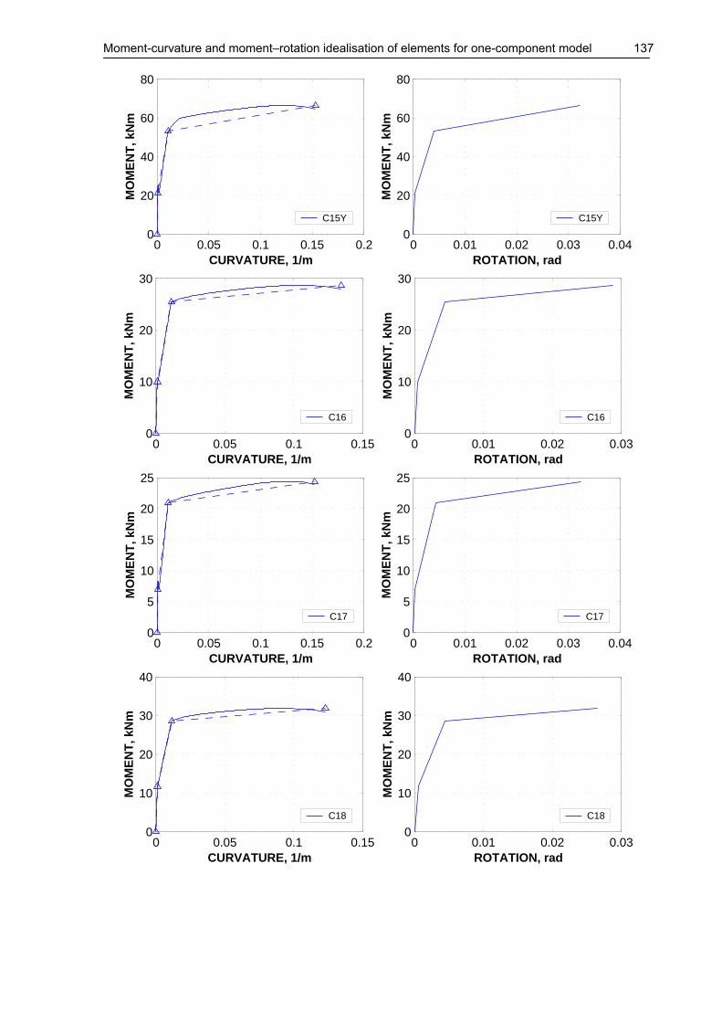
Moment-curvature and moment–rotation idealisation of elements for one-component model 137
0 0.05 0.1 0.15 0.20
20
40
60
80
CURVATURE, 1/m
MO
ME
NT
, kN
m
C15Y
0 0.01 0.02 0.03 0.040
20
40
60
80
ROTATION, rad
MO
ME
NT
, kN
m
C15Y
0 0.05 0.1 0.150
10
20
30
CURVATURE, 1/m
MO
ME
NT
, kN
m
C16
0 0.01 0.02 0.030
10
20
30
ROTATION, rad
MO
ME
NT
, kN
m
C16
0 0.05 0.1 0.15 0.20
5
10
15
20
25
CURVATURE, 1/m
MO
ME
NT
, kN
m
C17
0 0.01 0.02 0.03 0.040
5
10
15
20
25
ROTATION, rad
MO
ME
NT
, kN
m
C17
0 0.05 0.1 0.150
10
20
30
40
CURVATURE, 1/m
MO
ME
NT
, kN
m
C18
0 0.01 0.02 0.030
10
20
30
40
ROTATION, rad
MO
ME
NT
, kN
m
C18

138 Moment-curvature and moment–rotation idealisation of elements for one-component model
0 0.05 0.1 0.150
10
20
30
CURVATURE, 1/m
MO
ME
NT
, kN
m
C19
0 0.01 0.02 0.030
10
20
30
ROTATION, rad
MO
ME
NT
, kN
m
C19
0 0.05 0.1 0.150
10
20
30
CURVATURE, 1/m
MO
ME
NT
, kN
m
C20
0 0.01 0.02 0.03 0.040
10
20
30
ROTATION, rad
MO
ME
NT
, kN
m
C20
0 0.05 0.1 0.150
10
20
30
40
CURVATURE, 1/m
MO
ME
NT
, kN
m
C21
0 0.01 0.02 0.030
10
20
30
40
ROTATION, rad
MO
ME
NT
, kN
m
C21
0 0.05 0.1 0.150
10
20
30
CURVATURE, 1/m
MO
ME
NT
, kN
m
C22
0 0.01 0.02 0.030
10
20
30
ROTATION, rad
MO
ME
NT
, kN
m
C22
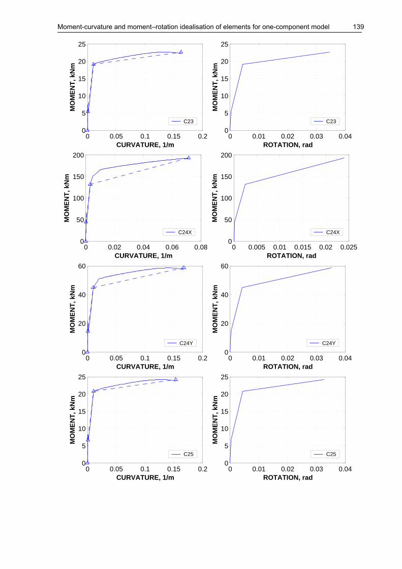
Moment-curvature and moment–rotation idealisation of elements for one-component model 139
0 0.05 0.1 0.15 0.20
5
10
15
20
25
CURVATURE, 1/m
MO
ME
NT
, kN
m
C23
0 0.01 0.02 0.03 0.040
5
10
15
20
25
ROTATION, rad
MO
ME
NT
, kN
m
C23
0 0.02 0.04 0.06 0.080
50
100
150
200
CURVATURE, 1/m
MO
ME
NT
, kN
m
C24X
0 0.005 0.01 0.015 0.02 0.0250
50
100
150
200
ROTATION, rad
MO
ME
NT
, kN
m
C24X
0 0.05 0.1 0.15 0.20
20
40
60
CURVATURE, 1/m
MO
ME
NT
, kN
m
C24Y
0 0.01 0.02 0.03 0.040
20
40
60
ROTATION, rad
MO
ME
NT
, kN
m
C24Y
0 0.05 0.1 0.15 0.20
5
10
15
20
25
CURVATURE, 1/m
MO
ME
NT
, kN
m
C25
0 0.01 0.02 0.03 0.040
5
10
15
20
25
ROTATION, rad
MO
ME
NT
, kN
m
C25
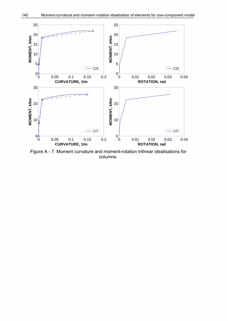
140 Moment-curvature and moment–rotation idealisation of elements for one-component model
0 0.05 0.1 0.15 0.20
5
10
15
20
25
CURVATURE, 1/m
MO
ME
NT
, kN
m
C26
0 0.01 0.02 0.03 0.040
5
10
15
20
25
ROTATION, rad
MO
ME
NT
, kN
m
C26
0 0.05 0.1 0.15 0.20
10
20
30
CURVATURE, 1/m
MO
ME
NT
, kN
m
C27
0 0.01 0.02 0.03 0.040
10
20
30
ROTATION, rad
MO
ME
NT
, kN
m
C27
Figure A - 7. Moment curvature and moment-rotation trilinear idealisations for
columns.

Determination of displacement demand by N2 method 141
ANNEX IV. Determination of displacement demand by N2 method
0 0.05 0.1 0.15 0.20
100
200
300
TOP DISPLACEMENT
BA
SE
SH
EA
RMODE1 100X−P
dataini−limmax−limini−fitmax−fityield forceBILINEAR
−0.25 −0.2 −0.15 −0.1 −0.05 0−300
−200
−100
0
TOP DISPLACEMENT
BA
SE
SH
EA
R
MODE1 100X−N
dataini−limmax−limini−fitmax−fityield forceBILINEAR
Figure A - 8. Bilinear idealisation of the capacity curves for the positive and negative
pushovers in the X direction, ETCP model.
0 0.05 0.1 0.150
1
2
3
4
5
Sd, m
Sa, m
/s2
MODE1 100X−N
Sd=0.065Γ=1.23Dt=−0.0801
El. spec. ag=1.96Inel. spec. µ=2.7SDOF capacity curve
0 0.05 0.1 0.150
1
2
3
4
5
Sd, m
Sa, m
/s2
MODE1 100X−P
Sd=0.062Γ=1.23Dt=0.0765
El. spec. ag=1.96Inel. spec. µ=2.89SDOF capacity curve
0 0.05 0.1 0.150
1
2
3
4
5
Sd, m
Sa, m
/s2
MODE1 100Y−N
Sd=0.0569Γ=1.26Dt=−0.0715
El. spec. ag=1.96Inel. spec. µ=2.32SDOF capacity curve
0 0.05 0.1 0.150
1
2
3
4
5
Sd, m
Sa, m
/s2
MODE1 100Y−P
Sd=0.0581Γ=1.26Dt=0.073
El. spec. ag=1.96Inel. spec. µ=2.76SDOF capacity curve
Figure A - 9. Determination of displacement demand of the equivalent SDOF system
by the N2 method, ETCP model, 0.2g intensity level.

142 Determination of displacement demand by N2 method
0 0.02 0.04 0.06 0.080
0.5
1
1.5
2
2.5
Sd, m
Sa,
m/s
2
MODE1 100X−P
Sd=0.031Γ=1.23Dt=0.0382
El. spec. ag=0.981Inel. spec. µ=1.44SDOF capacity curve
0 0.02 0.04 0.06 0.080
0.5
1
1.5
2
2.5
Sd, m
Sa,
m/s
2
MODE1 100Y−P
Sd=0.0291Γ=1.26Dt=0.0365
El. spec. ag=0.981Inel. spec. µ=1.38SDOF capacity curve
Figure A - 10. Determination of displacement demand of the equivalent SDOF
system by the N2 method, ETCP model, 0.1g intensity level.
0 0.05 0.1 0.15 0.2 0.250
2
4
6
8
Sd, m
Sa, m
/s2
MODE1 100X−P
Sd=0.0931Γ=1.23Dt=0.115
El. spec. ag=2.94Inel. spec. µ=4.33SDOF capacity curve
0 0.05 0.1 0.15 0.2 0.250
2
4
6
8
Sd, m
Sa, m
/s2
MODE1 100Y−P
Sd=0.0872Γ=1.26Dt=0.11
El. spec. ag=2.94Inel. spec. µ=4.13SDOF capacity curve
Figure A - 11. Determination of displacement demand of the equivalent SDOF
system by the N2 method, ETCP model, 0.3g intensity level.
0 0.05 0.1 0.15 0.20
50
100
150
200
250
TOP DISPLACEMENT
BA
SE
SH
EA
R
MODE1 100X−P
dataini−limmax−limini−fitmax−fityield forceBILINEAR
−0.2 −0.15 −0.1 −0.05 0−300
−200
−100
0
TOP DISPLACEMENT
BA
SE
SH
EA
R
MODE1 100X−N
dataini−limmax−limini−fitmax−fityield forceBILINEAR
Figure A - 12. Bilinear idealisation of the capacity curves for the positive and negative
pushovers in the X direction, EFCP model.

Determination of displacement demand by N2 method 143
0 0.05 0.1 0.150
1
2
3
4
5
Sd, m
Sa, m
/s2
MODE1 100X−N
Sd=0.0774Γ=1.23Dt=−0.0954
El. spec. ag=1.96Inel. spec. µ=2.14SDOF capacity curve
0 0.05 0.1 0.150
1
2
3
4
5
Sd, m
Sa, m
/s2
MODE1 100X−P
Sd=0.0739Γ=1.23Dt=0.0911
El. spec. ag=1.96Inel. spec. µ=2.32SDOF capacity curve
0 0.05 0.1 0.150
1
2
3
4
5
Sd, m
Sa, m
/s2
MODE1 100Y−N
Sd=0.0687Γ=1.26Dt=−0.0864
El. spec. ag=1.96Inel. spec. µ=1.76SDOF capacity curve
0 0.05 0.1 0.150
1
2
3
4
5
Sd, m
Sa, m
/s2
MODE1 100Y−P
Sd=0.071Γ=1.26Dt=0.0893
El. spec. ag=1.96Inel. spec. µ=2.09SDOF capacity curve
Figure A - 13. Determination of displacement demand of the equivalent SDOF
system by the N2 method, EFCP model, 0.2g intensity level.
0 0.02 0.04 0.06 0.080
0.5
1
1.5
2
2.5
Sd, m
Sa,
m/s
2
MODE1 100X−P
Sd=0.037Γ=1.23Dt=0.0456
El. spec. ag=0.981Inel. spec. µ=1.16SDOF capacity curve
0 0.02 0.04 0.06 0.080
0.5
1
1.5
2
2.5
Sd, m
Sa,
m/s
2
MODE1 100Y−P
Sd=0.0355Γ=1.26Dt=0.0446
El. spec. ag=0.981Inel. spec. µ=1.04SDOF capacity curve
Figure A - 14. Determination of displacement demand of the equivalent SDOF
system by the N2 method, EFCP model, 0.1g intensity level.

144 Determination of displacement demand by N2 method
0 0.05 0.1 0.15 0.2 0.250
2
4
6
8
Sd, m
Sa, m
/s2
MODE1 100X−P
Sd=0.111Γ=1.23Dt=0.137
El. spec. ag=2.94Inel. spec. µ=3.48SDOF capacity curve
0 0.05 0.1 0.15 0.2 0.250
2
4
6
8
Sd, m
Sa, m
/s2
MODE1 100Y−P
Sd=0.107Γ=1.26Dt=0.134
El. spec. ag=2.94Inel. spec. µ=3.13SDOF capacity curve
Figure A - 15. Determination of displacement demand of the equivalent SDOF
system by the N2 method, EFCP model, 0.3g intensity level.
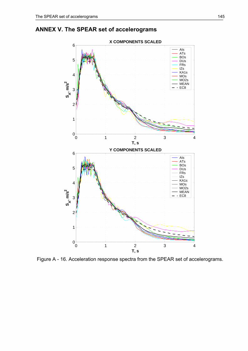
The SPEAR set of accelerograms 145
ANNEX V. The SPEAR set of accelerograms
0 1 2 3 40
1
2
3
4
5
6
T, s
SA
, m/s
2
X COMPONENTS SCALED
AIsATsBOsDUsFRsIZsKA1sMOsMO2sMEANEC8
0 1 2 3 40
1
2
3
4
5
6
T, s
SA
, m/s
2
Y COMPONENTS SCALED
AIsATsBOsDUsFRsIZsKA1sMOsMO2sMEANEC8
Figure A - 16. Acceleration response spectra from the SPEAR set of accelerograms.

146 The SPEAR set of accelerograms
0 5 10 15−4
−2
0
2
4
1.6
−2.94
TIME, s
X C
OM
PO
NE
NT
, m/s
2
ACCELERATION TIME HISTORY − AIs (AIs )
maxmin
0 5 10 15−4
−2
0
2
43
−1.56
TIME, s
Y C
OM
PO
NE
NT
, m/s
2
ACCELERATION TIME HISTORY − AIs (AIs )
maxmin
0 5 10 15−4
−2
0
2
4
2.15
−1.77
TIME, s
X C
OM
PO
NE
NT
, m/s
2
ACCELERATION TIME HISTORY − ATs (ATs )
maxmin
0 5 10 15−4
−2
0
2
4
2.03
−2.69
TIME, s
Y C
OM
PO
NE
NT
, m/s
2
ACCELERATION TIME HISTORY − ATs (ATs )
maxmin

The SPEAR set of accelerograms 147
0 5 10 15−4
−2
0
2
4
2.39
−1.58
TIME, s
X C
OM
PO
NE
NT
, m/s
2
ACCELERATION TIME HISTORY − BOs (BOs )
maxmin
0 5 10 15−4
−2
0
2
43.12
−1.79
TIME, s
Y C
OM
PO
NE
NT
, m/s
2
ACCELERATION TIME HISTORY − BOs (BOs )
maxmin
0 5 10 15−4
−2
0
2
4
1.62
−1.66
TIME, s
X C
OM
PO
NE
NT
, m/s
2
ACCELERATION TIME HISTORY − DUs (DUs )
maxmin
0 5 10 15−4
−2
0
2
4
2.44
−1.72
TIME, s
Y C
OM
PO
NE
NT
, m/s
2
ACCELERATION TIME HISTORY − DUs (DUs )
maxmin

148 The SPEAR set of accelerograms
0 5 10 15−4
−2
0
2
4
2.45
−1.49
TIME, s
X C
OM
PO
NE
NT
, m/s
2
ACCELERATION TIME HISTORY − FRs (FRs )
maxmin
0 5 10 15−4
−2
0
2
4
1.69
−1.69
TIME, s
Y C
OM
PO
NE
NT
, m/s
2
ACCELERATION TIME HISTORY − FRs (FRs )
maxmin
0 5 10 15−4
−2
0
2
4
2.48
−1.7
TIME, s
X C
OM
PO
NE
NT
, m/s
2
ACCELERATION TIME HISTORY − IZs (IZs )
maxmin
0 5 10 15−4
−2
0
2
4
1.94
−2.77
TIME, s
Y C
OM
PO
NE
NT
, m/s
2
ACCELERATION TIME HISTORY − IZs (IZs )
maxmin

The SPEAR set of accelerograms 149
0 5 10 15−4
−2
0
2
4
2.12
−1.93
TIME, s
X C
OM
PO
NE
NT
, m/s
2
ACCELERATION TIME HISTORY − KA1s (KA1s )
maxmin
0 5 10 15−4
−2
0
2
4
1.62
−2.24
TIME, s
Y C
OM
PO
NE
NT
, m/s
2
ACCELERATION TIME HISTORY − KA1s (KA1s )
maxmin
0 5 10 15−4
−2
0
2
4
2.59
−1.78
TIME, s
X C
OM
PO
NE
NT
, m/s
2
ACCELERATION TIME HISTORY − MO2s (MO2s )
maxmin
0 5 10 15−4
−2
0
2
4
1.96
−2.33
TIME, s
Y C
OM
PO
NE
NT
, m/s
2
ACCELERATION TIME HISTORY − MO2s (MO2s )
maxmin
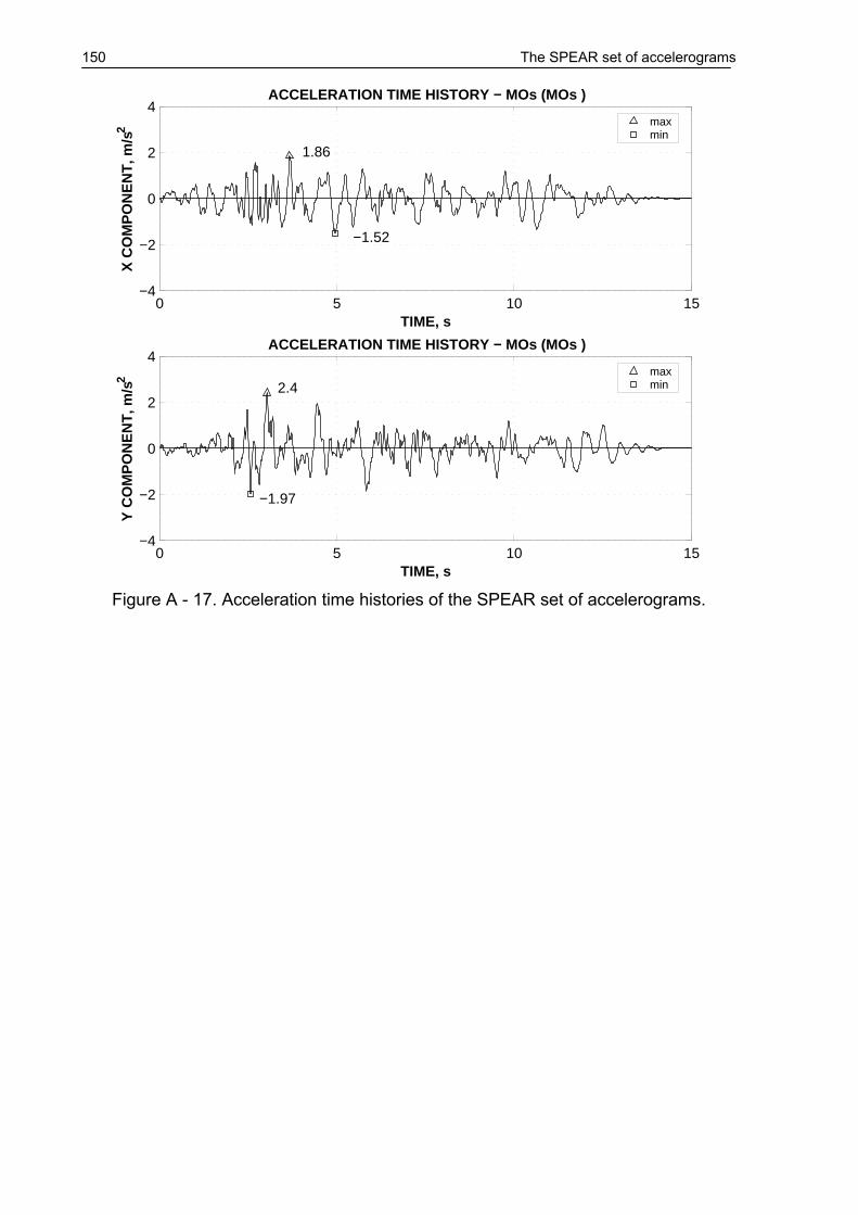
150 The SPEAR set of accelerograms
0 5 10 15−4
−2
0
2
4
1.86
−1.52
TIME, s
X C
OM
PO
NE
NT
, m/s
2
ACCELERATION TIME HISTORY − MOs (MOs )
maxmin
0 5 10 15−4
−2
0
2
4
2.4
−1.97
TIME, s
Y C
OM
PO
NE
NT
, m/s
2
ACCELERATION TIME HISTORY − MOs (MOs )
maxmin
Figure A - 17. Acceleration time histories of the SPEAR set of accelerograms.


![Khamael Spear[1]](https://img.dokumen.tips/doc/110x75/577cdada1a28ab9e78a6b67c/khamael-spear1.jpg)