Embed Size (px)
Citation preview

Segmented Asset Markets and Optimal Exchange Rate
Regimes1
Amartya Lahiri
Federal Reserve Bank of New York
Rajesh Singh
Iowa State University
Carlos Vegh
UCLA and NBER
Revised: June 2004
1 We would like to thank Andy Atkeson, Mick Devereaux, Huberto Ennis, Andy Neumeyer, Mark Spiegel,
and seminar participants at Duke, FRB Cleveland, FRB NY, Penn State, UBC, UCLA, UC Santa Cruz,
USC, Warwick, CMSG 2003, ITAM-FBBVA Summer Camp 2003, SED 2003, NBER IFM meeting Fall 2003,
for helpful comments and suggestions. The usual disclaimer applies. Végh would like to thank the UCLA
Academic Senate for research support. The views expressed here do not necessarily reflect the views of the
Federal Reserve Bank of New York or the Federal Reserve System.

Abstract
This paper revisits the issue of the optimal exchange rate regime in a flexible price environment.
The key innovation is that we analyze this question in the context of environments where only
a fraction of agents participate in asset market transactions (i.e., asset markets are segmented).
We show that flexible exchange rates are optimal under monetary shocks and fixed exchange rates
are optimal under real shocks. These findings are the exact opposite of the standard Mundellian
prescription derived under the sticky price paradigm wherein fixed exchange rates are optimal if
monetary shocks dominate while flexible rates are optimal if shocks are mostly real. Our results
thus suggest that the optimal exchange rate regime should depend not only on the type of shock
(monetary versus real) but also on the type of friction (goods market friction versus financial market
friction).
Keywords: Optimal exchange rates, asset market segmentation
JEL Classification: F1, F2
1 Introduction
Fifty years after Milton Friedman’s (1953) celebrated case for flexible exchange rates, the debate
on the optimal choice of exchange rate regimes rages on as fiercely as ever. Friedman argued
that, in the presence of sticky prices, floating rates would provide better insulation from foreign
shocks by allowing relative prices to adjust faster. In a world of capital mobility, Mundell’s (1963)
work implies that the optimal choice of exchange rate regime should depend on the type of shocks
hitting an economy: real shocks would call for a floating exchange rate, whereas monetary shocks
would call for a fixed exchange rate. Ultimately, however, an explicit cost/benefit comparison
of exchange rate regimes requires a utility-maximizing framework, as argued by Helpman (1981)
and Helpman and Razin (1979). In such a framework, Engel and Devereux (1998) reexamine
this question in a sticky prices model and show how results are sensitive to whether prices are
denominated in the producer’s or consumer’s currency. On the other hand, Cespedes, Chang, and
Velasco (2000) incorporate liability dollarization and balance sheets effects and conclude that the
standard prescription in favor of flexible exchange rates in response to real shocks is not essentially
affected.
An implicit assumption in most, if not all, of the literature is that economic agents have un-
restricted and permanent access to asset markets.1 This, of course, implies that in the absence
of nominal rigidities, the choice of fixed versus flexible exchange rates is irrelevant. In practice,
however, access to asset markets is limited to some fraction of the population (due to, for example,
fixed costs of entry). This is likely to be particularly true in developing countries where asset mar-
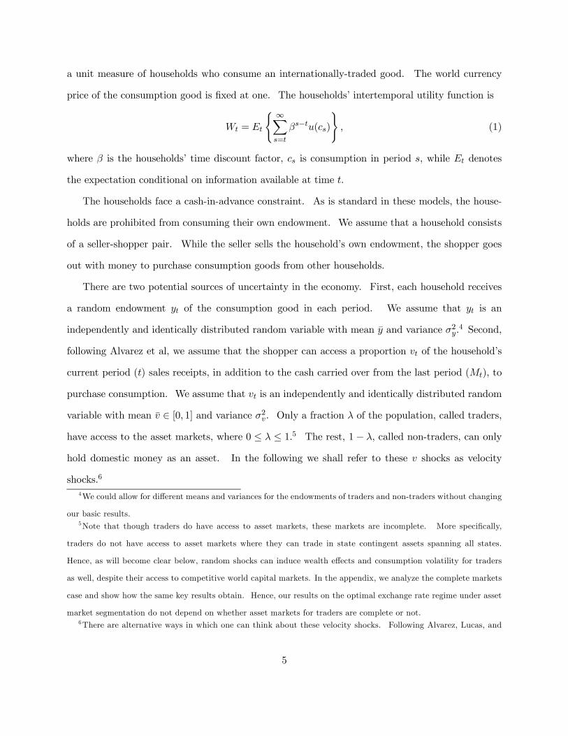
kets are much smaller in size than in industrial countries. Table 1 shows that even for the United
States, the degree of segmentation in asset markets is remarkably high. The table reveals that
59 percent of U.S. households did not hold any interest bearing assets (defined as money market
accounts, certificates of deposit, bonds, mutual funds, and equities). More strikingly, 25 percent
1There are some exceptions when it comes to the related issue of the costs and benefits of a common currency
area (see, for example, Neumeyer (1998) and Ching and Devereux (2000), who analyze this issue in the presence of
incomplete asset markets).
1

of households did not even have a checking account as late as in 1989. Given these facts for a
developed country like the United States, it is easy to anticipate that the degree of asset market
segmentation in emerging economies must be considerably higher. Since asset markets are at the
heart of the adjustment process to different shocks in an open economy, it would seem natural to
analyze how asset market segmentation affects the choice of exchange rate regime.2
Table 1: US Household ownership of financial assets, 1989
Interest-bearing assets
Checking account No Yes Total
No 19% 6% 25%
Yes 40% 35% 75%
Total 59% 41% 100%
Source: Mulligan and Sala-i-Martin (2000). Data from the Survey of Consumer Finance.
This paper abstracts from any nominal rigidity and focuses on a standard monetary model of an
economy subject to stochastic real and monetary (i.e., velocity) shocks in which the only friction
is that an exogenously-given fraction of the population can access asset markets. The analysis
makes clear that asset market segmentation introduces a fundamental asymmetry in the choice of
fixed versus flexible exchange rates. To see this, consider first the effects of a positive velocity
shock in a standard one-good open economy model in the absence of asset market segmentation.
Under flexible exchange rates, the velocity shock gets reflected in an excess demand for goods,
which leads to an increase in the price level (i.e., the exchange rate). Under fixed exchange rates,
2 In closed economy macroeconomics, asset market segmentation has received widespread attention ever since the
pioneering work of Grossman and Weiss (1983) and Rotemberg (1984) (see also Chatterjee and Corbae (1992) and
Alvarez, Lucas, and Weber (2001)). The key implication of these models is that open market operations reduce the
nominal interest rate and thereby generate the so-called “liquidity effect”. In an open economy context, Alvarez and
Atkeson (1997) and Alvarez, Atkeson, and Kehoe (2002) have argued that asset market segmentation models help in
resolving outstanding puzzles in international finance such as volatile and persistent real exchange rate movements
as well as excess volatility of nominal exchange rates.
2

the adjustment must take place through an asset market operation whereby agents exchange their
excess money balances for foreign bonds at the central bank. In either case, the adjustment
takes place instantaneously with no real effects. How does asset market segmentation affect this
adjustment? Under flexible rates, the same adjustment takes place. Under fixed exchange rates,
however, only those agents who have access to asset markets (called “traders”) may get rid of
their excess money balances. Non-traders — who are shut off from assets markets — cannot do this.
Non-traders are therefore forced to buy excess goods. The resultant volatility of consumption is
costly from a welfare point of view. Hence, under asset market segmentation and in the presence
of monetary shocks, flexible exchange rates are superior than fixed exchange rates.
Asset market segmentation also has dramatic implications for the optimal exchange rate regime
when shocks come from the goods market. We show that when output is stochastic, non-traders
in the economy unambiguously prefer fixed exchange rates to flexible exchange rates because pegs
provide a form of risk pooling. Under a peg, household consumption is a weighted average of
current period and last period’s output which implies that the consumption risk of non-trading
households is pooled across periods. Under flexible rates, however, the real value of consumption
is always current output which implies no intertemporal risk sharing. Trading households, on the
other hand, prefer flexible exchange rates to fixed exchange rates since maintaining an exchange
rate peg involves injecting or withdrawing money from traders which makes their consumption more
volatile under a peg. However, using a population share weighted average of the welfare of the
two types, we show that under fairly general conditions, the non-traders’ preferences dominate the
social welfare function. Hence, when output is stochastic, an exchange rate peg welfare dominates
a flexible exchange rate regime.3
In sum, the paper shows that asset market segmentation may be a critical friction in determining
the optimal exchange rate regime. More crucially, results under asset market segmentation run
3We derive the results in the text under incomplete markets, which is the more realistic assumption (see Burnside,
Eichenbaum, and Rebelo (1999) for a related discussion.) We show in the appendix that the same results obtain
under complete markets (and, are in fact, even starker).
3
counter to the Mundellian prescription that if monetary shocks dominate then fixed rates are
preferable, while if real shocks dominate flexible rates are preferable. This discrepancy reflects the
difference in the underlying friction. In the Mundell-Fleming world, sticky prices presumably reflect
some imperfection in goods markets, whereas in our model asset market segmentation captures some
imperfection in asset markets (for example, fixed cost of entry). Of course, which friction dominates
in practice is ultimately an empirical issue. However, our results suggest that policy judgements
regarding the choice of exchange rate regimes need to be based on a broader set of analytical factors
than just the standard sticky price-based Mundell insight. In particular, aside from a judgement
regarding the relative importance of alternative shocks (e.g., monetary or real shocks), this decision
should also be based on a judgement regarding the relative importance of alternative frictions (e.g.,
sticky prices or asset market segmentation) since different frictions have conflicting implications.
Lastly, we also study the implications of asset market segmentation for the debate regarding
inflation targeting versus money targeting. Since most of the existing work on this topic has been
done in a closed economy context, we study the question in that context as well. Mirroring the
results in the open economy version, we find that under asset market segmentation, money-targeting
is welfare superior to inflation targeting when shocks are monetary while inflation targeting is the
superior policy if shocks are real.
The paper proceeds as follows. Section 2 presents the model and the equilibrium conditions
while Section 3 describes the allocations under alternative exchange rate regimes and derives the
optimal regime under monetary and output shocks. Section 4 studies the implications of asset
market segmentation for the inflation targeting versus money targeting debate in a closed economy
context. Finally, Section 5 concludes. Algebraically tedious proofs are consigned to an appendix.
The appendix also derives the complete markets case.
2 Model
The basic model is an open economy variant of the model outlined in Alvarez, Lucas, and Weber
(2001). Consider a small open economy perfectly integrated with world goods markets. There is
4
a unit measure of households who consume an internationally-traded good. The world currency
price of the consumption good is fixed at one. The households’ intertemporal utility function is
Wt = Et
( ∞Xs=t
βs−tu(cs)
), (1)
where β is the households’ time discount factor, cs is consumption in period s, while Et denotes
the expectation conditional on information available at time t.
The households face a cash-in-advance constraint. As is standard in these models, the house-
holds are prohibited from consuming their own endowment. We assume that a household consists
of a seller-shopper pair. While the seller sells the household’s own endowment, the shopper goes
out with money to purchase consumption goods from other households.
There are two potential sources of uncertainty in the economy. First, each household receives
a random endowment yt of the consumption good in each period. We assume that yt is an
independently and identically distributed random variable with mean y and variance σ2y.4 Second,
following Alvarez et al, we assume that the shopper can access a proportion vt of the household’s
current period (t) sales receipts, in addition to the cash carried over from the last period (Mt), to
purchase consumption. We assume that vt is an independently and identically distributed random
variable with mean v ∈ [0, 1] and variance σ2v. Only a fraction λ of the population, called traders,
have access to the asset markets, where 0 ≤ λ ≤ 1.5 The rest, 1− λ, called non-traders, can only
hold domestic money as an asset. In the following we shall refer to these v shocks as velocity
shocks.6
4We could allow for different means and variances for the endowments of traders and non-traders without changing
our basic results.5Note that though traders do have access to asset markets, these markets are incomplete. More specifically,
traders do not have access to asset markets where they can trade in state contingent assets spanning all states.
Hence, as will become clear below, random shocks can induce wealth effects and consumption volatility for traders
as well, despite their access to competitive world capital markets. In the appendix, we analyze the complete markets
case and show how the same key results obtain. Hence, our results on the optimal exchange rate regime under asset
market segmentation do not depend on whether asset markets for traders are complete or not.6There are alternative ways in which one can think about these velocity shocks. Following Alvarez, Lucas, and
5
The timing runs as follows. First, both the endowment and velocity shocks are realized at
the beginning of every period. Second, the household splits. Sellers of both households stay at
home and sell their endowment for local currency. Shoppers of the non-trading households are
excluded from the asset market and, hence, go directly to the goods market with their overnight
cash to buy consumption goods. Shoppers of trading households first carry the cash held overnight
to the asset market where they trade in bonds and receive any money injections for the period.
They then proceed to the goods market with whatever money balances are left after their portfolio
rebalancing. After acquiring goods in exchange for cash, the non-trading-shopper returns straight
home while.the trading-shopper can re-enter the asset market to exchange goods for foreign bonds.
After all trades for the day are completed and markets close, the shopper and the seller are reunited
at home.
2.1 Households’ problem
2.1.1 Non-traders
The non-trader’s cash-in-advance constraint is given by:
MNTt + vtStyt = Stc
NTt , (2)
where MNTt is the beginning of period t nominal money balances while St is the period t exchange
rate (the domestic currency price of foreign currency). Equation (2) shows that for consumption
purposes, the non-traders can augment the beginning of period cash balances by withdrawals from
current period sales receipts vt (the velocity shocks). Money balances at the beginning of period
t+ 1 are given by sales receipts net of withdrawals for period t consumption:
MNTt+1 = Styt(1− vt), (3)
Weber (2001) one can ‘think of the shopper as visiting the seller’s store at some time during the trading day, emptying
the cash register, and returning to shop some more’. The uncertainty regarding v can be thought of as the uncertainty
regarding the total volume of sales at the time that the shopper accesses the cash register. Alternatively, one can
think of this as representing an environment where the shopper can purchase goods either through cash or credit.
However, the mix of cash and credit transactions is uncertain and fluctuates across periods.
6

where St denotes the domestic currency price of consumption goods at time t.
The usual flow constraint follows from combining (2) and (3):
MNTt+1 =MNT
t + Styt − StcNTt . (4)
Given the cash-in-advance (2), it follows that:
cNTt =
MNTt + vtStyt
St. (5)
2.1.2 Traders
The traders begin any period with assets in the form of money balances and bond holdings carried
over from the previous period. Armed with these assets the shopper of the trader household visits
the asset market where she rebalances the household’s asset position and also receives the lump
sum asset market transfers from the government. Thus, for any period t, the accounting identity
for the asset market transactions of a trader household is given by
MTt =MT
t + (1 + it−1)Bt
λ− Bt+1
λ+ St(1 + r)ft − Stft+1 +
Ttλ, (6)
where MTt denotes the money balances with which the trader leaves the asset market and MT
t
denotes the money balances with which the trader entered the asset market. Also, B denotes
aggregate one-period nominal government bonds, i is the interest rate on these nominal bonds, f
are foreign bonds (denominated in terms of the consumption good), r is the exogenous and constant
world real interest rate, and T are aggregate (nominal) lump-sum transfers (i.e., negative taxes)
from the government.7,8 Note that nominal bonds maturing at date t pay an interest rate it−1 since7We assume that these transfers are made in the asset markets, where only the traders are present. Note that
since B and T denote aggregate bonds and aggegate transfers, their corresponding per trader values are B/λ and
T/λ since traders comprise a fraction λ of the population.8The assumption of endogenous lump-sum transfers will ensure that any monetary policy may be consistent with
the intertemporal fiscal constraint. This becomes particularly important in this stochastic environment where these
endogenous transfers will have to adjust to ensure intertemporal solvency for any history of shocks. To make our
life easier, these transfers are assumed to go only to traders. If these transfers also went to non-traders, then (5)
would be affected.
7

this rate was contracted in t − 1.9 After asset markets close, the shopper proceeds to the goods
market with MT in nominal money balances to purchase consumption goods. Like non-traders,
traders can also augment these starting money balances with random withdrawals from current
sales receipts to carry out goods purchases. Thus, the cash-in-advance constraint for a trader is
given by10
StcTt = MT
t + vtStyt. (7)
Combining equations (6) and (7) gives
MTt +
Ttλ+ vtStyt = Stc
Tt +
Bt+1
λ− (1 + it−1)
Bt
λ+ Stft+1 − St(1 + r)ft, (8)
In this set-up the only reason that traders hold money overnight is the separation between
markets. In particular, if the seller could access the asset market at the end of the day, then the
trading household would use all their remaining sales receipts from the period to buy interest bearing
bonds. However, since asset markets close before the opening of the goods market, traders are
forced to hold money overnight. Thus, period-t sales receipts net of withdrawals become beginning
of next period’s money balances
MTt+1 = Styt(1− vt). (9)
Note that since v, S, and y are all exogenous, the traders’ money holdings evolve exogenously over
time.
A trader chooses ct, Bt+1 and ft+1 to maximize (1) subject to the flow constraint (8). Combining
first-order conditions, we obtain:
u0(cTt ) =β(1 + r)Et
©u0(cTt+1)
ª, (10)
u0(cTt )St
=β (1 + it)Et
"u0(cTt+1)St+1
#. (11)
9Alternatively, we could work with one period discount bonds so that the time t price of a bond paying one unit
of the local at time t+ 1 would be 11+it
.10Throughout the analysis we shall restrict attention to ranges in which the cash-in-advance constraint binds for
both traders and non-traders. In general, this would entail checking the individual optimality conditions to infer the
parameter restrictions for which the cash-in-advance constraints bind.
8

Equation (10) is the standard Euler equation for the trader which relates the expected marginal
rate of consumption substitution between today and tomorrow to the return on savings (given by
1 + r) discounted to today. Equation (11), on the other hand, determines the optimal holdings of
nominal bonds. Equations (10) and (11) jointly determine the modified interest parity condition
for this economy which reflects the standard portfolio choice between safe and risky assets.
2.2 Government
The government in this economy holds foreign bonds (reserves) which earn the world rate of interest
r. The government can sell nominal domestic bonds, issue domestic money, and make lump sum
transfers to the traders. Thus, the government’s budget constraint is given by
Stht+1 − (1 + r)Stht + (1 + it−1)Bt −Bt+1 + Tt =Mt+1 −Mt, (12)
where B denotes the amount of nominal government bonds held by the private sector, h are foreign
bonds held by the government, M is the aggregate money supply, and T is government transfers
to the traders. Equation (12) makes clear that the money supply can be altered in three ways:
through open market operations, through interventions in the foreign exchange market, or through
transfers. Importantly, all three methods impact only the traders since they are the only agents
present in the asset market.
2.3 Equilibrium conditions
Equilibrium in the money market requires that
Mt = λMTt + (1− λ)MNT
t . (13)
The flow constraint for the economy as a whole (i.e., the current account) follows from combining the
flow constraint for non-traders (equation (4)), traders (equations (7) and (9)), and the government
(equation (12)) and money market equilibrium (equation (13)):
λcTt + (1− λ)cNTt = yt + (1 + r)kt − kt+1, (14)
where k ≡ h+ λf denotes per-capita foreign bonds for the economy as a whole.
9

To obtain the quantity theory, combine (3), (9) and (13) to get:
Mt+1
1− vt= Styt. (15)
Notice that the stock of money relevant for the quantity theory is end of period t money balances
(i.e., Mt+1). This reflects the fact that, unlike standard CIA models (in which the goods market is
open before the asset market and shoppers cannot withdraw current sales receipts for consumption),
in this model (i) asset markets open and close before goods market open (which allows traders to
change this period’s money balances for consumption purposes); and (ii) both traders and non-
traders can access current sales receipts.
Combining (3) and (5) gives the consumption of non-traders:
cNTt =
St−1yt−1 + (vtStyt − vt−1St−1yt−1)St
. (16)
To derive the consumption of traders, we use equation (9) to substitute for MTt in equation (8).
Then, subtracting Styt from both sides allows us to rewrite (8) as
(1 + r)ft − ft+1 +(1 + it−1)Bt
λ − Bt+1
λ + Ttλ
St+ yt − cTt =
Mt+1 −Mt
St,
where we have used equation (15) to getMt+1−Mt = [(Styt − St−1yt−1)− (vtStyt − vt−1St−1yt−1)].
Using equation (12) in the equation above gives
kt+1λ− (1 + r)
ktλ= yt − cTt +
µ1− λ
λ
¶µMt+1 −Mt
St
¶, (17)
where k0 is given exogenously. Equation (17) gives the trader’s flow constraint in equilibrium. The
left hand side captures the net acquisition of foreign assets (per trader) by the economy while the
right hand side gives periodic trader income net of consumption. Given the precise monetary regime,
we can iterate forward equation (17) and impose the trader household’s first order condition for
optimal consumption (equation (10)) to derive the trader’s policy function for consumption along
a rational expectations equilibrium path.
It is worth noting that the last term on the right hand side of (17) captures the source of
redistribution in this economy. Any changes of money supply occur through central bank operations
10

in the asset market where only traders are present. Hence, the traders receive the entire incremental
money injection while their own increase in money balances is only a fraction λ of the total. This
leads to redistribution of¡1−λλ
¢³Mt+1−Mt
St
´from non-traders to traders. Note that as λ→ 1 this
term goes to zero. It is important to note that this channel exists solely due to asset market
segmentation.
3 Alternative exchange rate regimes
Having described the model and the equilibrium conditions above, we now turn to allocations
under specific exchange rate regimes. We will look at two pure cases: flexible exchange rates and
fixed exchange rates. The end goal, of course, is to evaluate the welfare implications under the
two regimes. In all the policy experiments below, we shall assume that the initial distribution of
nominal money balances across the two types of agents is invariant. In particular, we assume that
MT0 =MNT
0 = M .
In order to make the analytics of the welfare comparisons tractable, we shall also assume from
hereon that the periodic utility function of both agents is quadratic:
u(c) = c− ζc2. (18)
To focus our results, we shall proceed by analyzing the effect of each shock in isolation. In
particular, we first study an environment where the only shock is the velocity shock and then go
to the other case where the only shock is the real shock.
3.1 Velocity shocks only
In this subsection we focus solely on velocity shocks. Hence, we set σ2y = 0. Thus, there is no
uncertainty about the endowment process. Every period all households receive the fixed endowment
y.
11
3.1.1 Flexible exchange rates under velocity shocks
We assume that under flexible exchange rates, the monetary authority sets a constant path of the
money supply:
Mt = M.
Further, the government does not intervene in foreign exchange markets and, for simplicity, we
assume that initial foreign reserves are zero. Then, the government’s flow constraint reduces to:
(1 + it−1)Bt −Bt+1 + Tt = 0. (19)
The quantity theory equation (15) determines the exchange rate:
St =M
(1− vt)y. (20)
The exchange rate will thus follow the velocity shock and be high (low) when the shock v is high
(low).
Using (20), consumption of non-traders (given by equation(16)) under flexible exchange rates
can be written as:
cNT,flext = y , t ≥ 0. (21)
Equation (21) shows that consumption of non-traders remains constant at all times. Intuitively,
under floating exchange rates, prices change in proportion to the velocity shocks. Since the velocity
shock is common to all agents, there is no redistribution of purchasing power between agents.
To determine consumption of traders under the floating exchange rate regime, we can iterate
forward equation (17) under the condition Mt = M to get
cT,flext = rk0λ+ y , t ≥ 0, (22)
where we have used the fact that under the quadratic utility specification adopted above, equation
(10) — which describes the optimal consumption plans for traders — reduces to c0 = E0(ct) for all
t > 0. Hence, under flexible exchange rates, consumption of traders is also constant over time.
The intuition is the same as before. Since, prices change in proportion to their velocity shock,
12

there are no real balance effects on the traders. Hence, their consumption remains invariant over
time.
3.1.2 Fixed exchange rates under velocity shocks
Under fixed exchange rates, the monetary authority sets a constant path of the exchange rate equal
to S. In particular, we assume that the nominal exchange rate is fixed at
S =M
(1− v)y. (23)
In effect, we are assuming that at time t = 0 the monetary authority pegs the exchange rate at the
deterministic equilibrium level.
Under this specification, it is easy to see from equation (16) that consumption of non-traders
under a fixed exchange rate is given by
cNT,pegt = y [1 + (vt − vt−1)] , (24)
cNT,peg0 = y [1 + (v0 − v)] . (25)
Equation (24) shows that under an exchange rate peg, consumption of non-traders will fluctuate
by the full amount of their velocity shock. Intuitively, velocity shocks change the nominal balances
that non-traders have available for consumption. Since the price level is now fixed, any change
in nominal balances also implies a one-for-one change in real balances and, hence, affects the
consumption of non-traders.
To determine the consumption of traders we again iterate forward on equation (17) by using
the Euler equation c0 = E0(ct) and after imposing the condition St = S for all t, we get
cT,peg0 = rk0λ+ y
"1 +
µ1− 1
λ
¶r
1 + r
"(v0 − v) +E0
( ∞Xt=1
µ1
1 + r
¶t
(vt − vt−1)
)##. (26)
In deriving (26) we have used the fact that under pegged exchange rates, equation (15) implies that
Mt+1 −Mt = −(vt − vt−1)Sy.11
11More generally, consumption of traders under fixed exchange rates at any point in time t > 1 is given by
cT,pegt = rktλ+ y
"1 +
µ1− 1
λ
¶Et
( ∞Xs=t
µ1
1 + r
¶s−t(vs − vs−1)
)#.
13
To understand the consumption function of traders, note that under fixed exchange rates,
the nominal value of GDP remains unchanged, i.e., Sty = Sy for all t. The quantity theory
relationship requires that aggregate nominal money balances plus the aggregate withdrawal from
current period sales be sufficient to purchase current nominal output. To keep nominal output
unchanged over time, any change in cash withdrawals from current receipts, i.e., vt 6= vt−1, must
be met by the monetary authority with an offsetting change in aggregate nominal money balances.
This intervention must happen through transactions in the asset market where only traders are
present. On a per trader basis then, the proportional change in nominal money balances needed
for keeping the exchange rate fixed is − 1λ(vt − vt−1). Thus, under fixed exchange rates, a velocity
shock of ∆v not only changes real balances of traders by the full amount but also changes their
real balances by − 1λ due to central bank intervention. The net effect is 1 − 1λ which is the term
that shows up in the coefficient on the velocity shocks in equation (26).
3.1.3 Optimal exchange rate regime
Having described allocations under the alternative exchange rate arrangements, we now turn to the
key focus of the paper: determination of the optimal exchange rate regime. We shall conduct our
analysis by comparing the unconditional expectation of lifetime welfare at time t = 0 (i.e., before
the revelation of any information at time 0). In terms of preliminaries, it is useful to define the
following:
W i,j =E
½Xβt·ci,jt − ζ
³ci,jt
´2¸¾, i = T,NT , j = flex, peg, (27)
W j =λWT,j + (1− λ)WNT,j , j = flex, peg. (28)
Equation (27) gives the welfare for each agent under a specific exchange rate regime where the
relevant consumption for each type of agent is given by the consumption functions derived above
for each regime. Equation (28) is the aggregate welfare for the economy under each regime which
is the sum of the regime specific individual welfares weighted by their population shares. Note
that the quadratic utility specification implies that the expected value of periodic utility can be
14

written as
E¡c− ζc2
¢= E(c)− ζ [E(c)]2 − ζV ar(c). (29)
where var(c) denotes the variance of consumption.
Proposition 1 When velocity shocks are the only source of uncertainty in the economy, the flexible
exchange rate regime welfare-dominates the fixed exchange rate regime for both agents and hence,
is the optimal exchange rate regime for the economy.
Proof. It is easy to see that E(cNT,flext ) = E(cNT,peg
t ) = y while E(cT,flex0 ) = E(cT,peg0 ) = r k0λ + y.
Hence, for both types of agents, expected consumption under the two regimes is identical. However,
V ar(cT,pegt ) > V ar(cT,flext ) = 0 and V ar(cNT,pegt ) > V ar(cNT,flex
t ) = 0 for all t. From the
expression for expected periodic utility given by (29), it then follows directly that
W i,f lex > W i,peg, i = T,NT.
Hence, welfare under flexible exchange rates is greater than welfare under fixed exchange rates for
both agents. Thus, aggregate welfare under flexible exchange rates is unambiguously greater than
under fixed rates.
Intuitively, under flexible exchange rates the adjustment of the price level is proportional to the
velocity shock of both agents. Hence, flexible exchange rates completely insulate the real balances
of both agents which allows them to smooth consumption completely. Under fixed exchange rate on
the other hand, a wealth redistribution occurs across agents due to velocity shocks. Specifically, in
order to keep the exchange rate unchanged, the monetary authority intervenes in the asset market
to accommodate the average effect of the velocity shock. This affects transfers to traders which
induces redistributions. Hence, consumption of non-traders fluctuates over time while consumption
of traders is affected by a wealth effect coming from asset market transfers.
We should note that in the special case where all agents are traders, i.e., λ = 1, our model reduces
to a standard representative agent, small open economy model with perfect capital mobility. To
determine the optimal exchange rate regime in this case we can focus exclusively on the welfare
comparison for traders across the two exchange rate regimes.
15

Proposition 2 When all agents in the economy are traders, i.e., λ = 1, the fixed and flexible
exchange rate regimes are welfare equivalent.
Proof. For λ = 1 it follows directly from equations (22) and (26) that
cT,flex0 = cT,peg0 = rk0 + y.
Hence, for λ = 1, consumption for traders is identical under both regimes. Moreover, since no
stochastic terms enter the consumption function, welfare of traders (and hence aggregate welfare
as well) must be identical under both regimes. Thus, welfare is independent of the exchange rate
regime.
This result is similar to the well known result of Helpman and Razin (1979) who showed the
welfare equivalence between fixed and flexible exchange rates for representative agent economies
with perfect capital mobility where agents are subject to cash-in-advance constraints. Intuitively,
under flexible exchange rates the price level adjusts exactly in proportion to the trader’s velocity
shock which leaves her real balances unchanged and thereby insulates her completely from any
wealth effects due to real balance fluctuations. Symmetrically, when exchange rates are fixed,
the monetary authority pegs the exchange rate by exactly offsetting the aggregate velocity shock
through a corresponding intervention in asset markets. When all agents are in the asset market, the
intervention amount in asset markets corresponds exactly to the size of the trader’s velocity shock
which leaves their real balances unchanged. As in the flexible exchange rate case, this intervention
effectively insulates traders from any wealth effects due to their velocity shocks. Hence, the two
regimes are identical from a welfare standpoint.
3.2 Output shocks only
We now turn to the issue of real shocks and their effects in this model. To focus on this issue, we
assume that vt = v for all t and σ2v = 0. In other words, there is no uncertainty regarding the
velocity realization. However, we now assume that output, yt, is i.i.d. with mean y and variance
σ2y.
16

To analyze the welfare trade-offs under fixed and flexible exchange rates we shall continue to
assume that under flexible exchange rates Mt = M for all t while under fixed exchange rates
St = S (= M/ (1− v) y).
The quantity theory equation in this case is given by
Mt+1
1− v= Styt.
Note that Mt = M implies that under a flexible exchange rate regime, nominal income is constant
over time. Hence, nominal money balances of both types are also constant over time.
The above implies that consumption allocations for non-traders under the two regimes, using
equation (16), are given by
cNT,flext = yt, (30)
cNT,pegt =(1− v) yt−1 + vyt. (31)
Note that in deriving equation (30) we have used the fact St−1yt−1 = Styt under flexible rates.
Similarly, iterating forward on the periodic budget constraint for the trading households, equation
(17), and imposing the relevant monetary regime on the result gives the consumption allocations
for traders under the two regimes:
cT,flext = rktλ+ (1− β)yt + βy, (32)
cT,pegt = rktλ+ (1− β)
·µλ−Ωλ
¶yt−1 +
µβ +
1− β
λΩ
¶yt
¸+ β
µβ +
1− β
λΩ
¶y, (33)
where Ω = [1− (1− λ) v]. It is easy to check that E(cNT,flext ) = E(cNT,peg
t ) = y and E³cT,flext
´=
E³cT,pegt
´= r k0λ +y. Hence, expected consumption of both types is identical under the two regimes.
However the variance of consumption is different. Specifically,
V ar(cNT,flext ) =σ2y, (34)
V ar(cNT,pegt ) =σ2y [1− 2v (1− v)] < σ2y, (35)
V ar(cNT,peg0 ) = v2σ2y < σ2y (36)
17

Hence, for non-trading households, consumption volatility is lower under a peg relative to a flexible
exchange rate regime. Given that expected consumption is identical under the two regimes while
volatility is lower under a peg, it follows that non-traders always prefer a fixed exchange rate regime
to a flexible rate regime when shocks are real.12
To understand the intuition, note that under flexible exchange rates, a constant path of nominal
money balances implies that the real value of last period’s sales (in terms of current prices) is always
equal to current output. Hence, current consumption (which is a weighted average of current and
last period’s real sales revenues) is just current output. Thus, the entire variance of current output
is reflected in the variance of current consumption. Under an exchange rate peg on the other hand,
the real value of last period’s sales is always last period’s output. Hence, current consumption
is a weighted average of last period and current period’s output. The resulting lower variance
of consumption under a peg reflects a form of risk pooling: the consumption risk is pooled across
periods.
The variance of consumption of trading households also differs across the two regimes. In the
appendix (6.1) we show that
V ar³cT,flext
´=hr2tβ2 + (1− β)2
iσ2y, (37)
V ar³cT,peg0
´= (1− β)2
µβ +
1− β
λΩ
¶2σ2y, (38)
V ar³cT,pegt
´= r2
h³(t− 1) (βA+C)2
´+ r2C2 + (1− β)2
¡A2 +B2
¢+ 2r (1− β)AC
iσ2y, (39)
where A = λ−Ωλ , B = β + 1−β
λ Ω, and C = Ωλ − (1− β)B.
Our welfare metric is given, as before, by equation (28). In order to compare welfare across
regimes we define ∆W ≡W flex −W peg. Substituting equations (34-39) in (27) and (28) gives
∆W = λ∆WT + (1− λ)∆WN =1
λ
¡c2λ
2 + c1λ+ c0¢, (40)
12We should note that this result is crucially dependent on the household being able to consume some fraction of
current sales, i.e., v > 0. If v = 0 then cNT,flext = yt and cNT,peg
t = yt−1. Hence, both expected consumption and
the variance of consumption would be identical under the two regimes.
18

where c2 = a2³(1− β)2 − 1+β
1−β´+2a
³11−β − (1− β)
´; c1 = −a2
³2 (1− β)2 − 1+β
1−β´−2a
³11−β − (1− β)
´;
c0 = a2 (1− β)2 ; and where a = 1− v.
Lemma 1 Equation (40) has two roots: λ1 = 1 and λ2 =a2(1−β)2
a2³(1−β)2− 1+β
1−β´+2a
³1
1−β−(1−β)´ .
Proof. See Appendix.
Lemma 2 β ∈ (0.5, 1] and v > 0 are jointly sufficient conditions for λ2 ∈ (0, 1).
Proof. See Appendix.
Proposition 3 When endowment shocks are the only source of uncertainty in the economy and
the conditions of Lemma 2 apply, the optimal exchange rate regime is a fixed exchange rate for all
λ > λ2 while flexible exchange rates are optimal for all λ < λ2.
Proof. See Appendix.
Thus, Proposition 3 shows that whenever the share of traders is above a critical threshold,
fixed exchange rates are the optimal regime under real shocks. Note that this lower threshold
goes to zero as v tends to unity. The striking feature of this result is that it is the opposite of
the conventional wisdom derived under sticky prices. Recall that under sticky prices and real
shocks, flexible exchange rates are optimal. Hence, once again the well-known optimal exchange
rate results due to Mundell appear to be turned on their heads. Note that the conditions of Lemma
2 are quite non-restrictive.
To understand the intuition behind this result, it is helpful to note that while both types
of agents face the same shock, their ability to cope with them is asymmetric. In particular,
trading households have an extra instrument — financial assets — with which to smooth out their
consumption flow in response to shocks. Thus, the welfare losses of traders in shifting from a
flexible exchange rate regime to a peg is always smaller than the corresponding loss of a non-
trading household moving from a peg to a flexible exchange rate regime. Thus, the preferences of
non-traders typically dominates the overall welfare criterion.
The only caveat to this intuition occurs for very small values of λ. In particular, when λ < λ2,
a very small number of trading households have to bear the burden of maintaining an exchange
19

rate peg for the entire economy by accepting all the monetary injections or withdrawals. Due to
their very small numbers, the resultant consumption volatility of traders under a peg becomes very
big. At the limit, consumption volatility of traders goes to infinity as λ tends to zero. However,
our simulations show that for most realistic parameter values, λ2 is very small (typically in the
second or third decimal point).13 Moreover, we also know that for λ = 0 the optimal regime is
a peg since non-trading households unambiguously prefer exchange rate pegs to flexible regimes.
Hence, typically the range in which flexible rates are optimal is very small. This suggests that
exchange rate pegs are, in general, the optimal regime under output shocks.
4 Closed economy case
We now turn our attention from exchange rate policy in an open economy to monetary policy in a
closed economy context. Over the past decade, an ongoing debate in monetary policy design has
been the relative merit of inflation targeting versus money targeting. Lately a consensus appears
to be emerging in favor of inflation targeting. Most such conclusions are however derived from
environments with nominal stickiness (either prices or wages) (see Clarida, Gertler and Gali (1999)
for an overview of this literature). The framework studied in this paper provides an alternative
structure within which this question can be asked. The reason the answers may be different is
because the key friction here is an asset market friction as opposed to the sticky price friction
analyzed by most of the existing literature on the topic.
The model is the same as the one analyzed above. In particular, the closed economy version is
identical to the model analyzed by Alvarez et al (2001). Relative to the open economy case, the
key difference is that in the closed economy version goods markets must clear internally. Hence,
λcTt + (1− λ)cNTt = yt, for all t. (41)
The non-trading household’s constraints remain unchanged relative to the open economy case.
13The simulation results are available from the authors on request.
20

Hence, consumption of non-traders is the same as before:
cNTt = (1− vt−1)
St−1yt−1St
+ vtyt, (42)
where St denotes the domestic nominal price level. The market clearing condition then gives
consumption of the traders:
cTt =
·1 +
µ1− λ
λ
¶µ1− cNT
t
yt
¶¸yt. (43)
The trading household’s budget constraint is the same as before except for the absence of foreign
bonds. Thus,
MTt +
Ttλ+ vtStyt = Stc
Tt +
Bt+1
λ− (1 + it−1)
Bt
λ. (44)
Optimal behavior by traders now entails satisfying just one condition (equation (11)) which deter-
mines the nominal interest i. It is easy to check that the quantity theory equation derived earlier
continues to hold. Hence, the price level is determined by equation (15). Lastly, the government’s
budget constraint is now given by
(1 + it−1)Bt −Bt+1 + Tt =Mt+1 −Mt, (45)
which is identical to the open economy case except for the fact that there are no foreign reserves,
h, in the closed economy case.
4.1 Inflation targeting versus money targeting
In order to study the welfare merits of inflation targeting as opposed to money targeting, we assume
that the two regimes are characterized by the following policy rules:
Inflation Targeting: St+1 = (1 + µ)St, S0 =(1 + µ)M
(1− v)y, (46)
Money Targeting: Mt+1 = (1 + µ)Mt, M0 = M. (47)
Note that under inflation targeting we assume that the central bank also announces (and delivers
through an appropriate choice of M1) the initial price level S0. The precise number for S0 that
we have assumed guarantees that the two regimes are symmetric in terms of the expected first
21

period price level. Moreover, to keep the regimes symmetric, we have also assumed that the rate
of growth of the relevant policy target is the same for both regimes.
4.1.1 Velocity shocks only
As before, we start by studying environments where the only source of uncertainty is the velocity
shock. Hence, we set σ2y = 0. Under our assumptions it is easy to check that consumption
allocations under inflation targeting are given by
cNT,πt =
·1
1 + µ+
µvt − vt−1
1 + µ
¶¸y,
cNT,π0 =
·1
1 + µ+
µv0 − v
1 + µ
¶¸y.
Note that once cNT is known, cT is determined from the market clearing condition (41). Similarly,
under money targeting consumption allocations are given by
cNT,mt =
·1
1 + µ+
µ
1 + µvt
¸y,
cNT,m0 =
·1
1 + µ+
µ
1 + µv0
¸y.
It can easily be checked that
E(cNT,πt ) =E(cNT,m
t ) =
µ1 + µv
1 + µ
¶y,
V ar(cNT,πt ) = y2
·1 +
1
(1 + µ)2
¸σ2v, V ar(cNT,π
0 ) = y2σ2v,
V ar(cNT,mt ) = y2
µµ
1 + µ
¶2σ2v = V ar(cNT,m
0 ).
Hence, V ar(cNT,πt ) > V ar(cNT,π
0 ) > V ar(cNT,mt ) = V ar(cNT,m
0 ). Since expected consumption
is identical under the two regimes while the variance of consumption is greater under inflation
targeting, equation (18) implies that all agents unambiguously prefer money targeting to inflation
targeting under monetary shocks.14
14Note that in the closed economy case, consumption of traders is given by cTt =h1 +
¡1−λλ
¢ ³1− cNTt
y
´iy. Hence,
greater consumption volatility for non-traders also implies greater consumption volatility for traders.
22

4.1.2 Output shocks only
The second case of interest is where the only randomness in the economy is due to uncertainty
about the endowment realization. Hence, we now assume that σ2v = 0. It is again straightforward
to verify that in this case the consumption allocations of the non-trading households under the
inflation targeting regime of equation (46) are given by
cNT,πt =
1− v
1 + µyt−1 + vyt ,
cNT,π0 =
1− v
1 + µy + vy0.
Correspondingly, under the money-targeting policy given by equation (47), the consumption allo-
cations are
cNT,mt =
·1− v
1 + µ+ v
¸yt ,
cNT,m0 =
·1− v
1 + µ+ v
¸y0.
It is easy to check that E(cNT,πt ) = E(cNT,m
t ) =h1−v1+µ + v
iy for all t ≥ 0. Thus, expected
consumption is identical across regimes for both agents. However, the variance of consumption is
different. In particular, it follows from the above that
V ar(cNT,πt ) =
"µ1− v
1 + µ
¶2+ v2
#σ2y, V ar(cNT,π
0 ) = v2σ2y,
V ar(cNT,mt ) =
·µ1− v
1 + µ
¶+ v
¸2σ2y = V ar(cNT,m
0 ).
Hence, V ar(cNT,mt ) > V ar(cNT,π
t ) for all t ≥ 0 from which it follows that both types unambiguouslyprefer inflation targeting to money targeting under real shocks.
5 Conclusion
The determination of the optimal exchange rate regime for an open economy is one of the oldest
issues in international economics. The single most influential idea in this context has been the
Mundellian prescription that if shocks facing the country are mostly monetary then fixed exchange
23

rates are optimal whereas flexible rates are optimal if the shocks are mostly real. The key friction
underlying Mundell’s results was the assumption of sticky prices in the goods market. In this
paper we have investigated the implications of frictions in the asset market as opposed to the goods
market.
We have shown that when only a fraction of agents trade in asset markets (i.e., asset markets
are segmented), the Mundellian prescription gets turned on its head. Fixing exchange rates
entails central bank interventions in the asset market where only a fraction of agents are present.
Hence, monetary shocks (shocks to velocity in our context) under fixed exchange rate regimes cause
redistributions across agents thereby generating consumption volatility. On the other hand, when
exchange rates are flexible, monetary shocks cause changes in the price level which insulate agents’
real balances. Thus, asset market segmentation causes an inherent welfare bias towards flexible
exchange rate regimes when shocks are monetary. We have also derived general conditions under
which fixed exchange rates unambiguously welfare dominate flexible rates when the economy faces
only output shocks, thereby overturning the well-know Mundellian prescription once again.
We believe that the key importance of our results lies in their calling into question the conven-
tional wisdom regarding the choice of exchange rate regimes. The conventional thinking on this
topic has followed the sticky-price insights of Mundell (1963). We believe that nominal frictions
are but one of many possible frictions in any economy. More troublingly, we have shown that an
alternative friction whereby there is segmentation in asset markets leads to the opposite conclusion
regarding the choice of exchange rate regimes. Since a judgement regarding which friction is more
important is ultimately an empirical issue and likely to be country-specific, the main implication of
this paper is that an evaluation of the relative strengths of alternative frictions must be a key input
into any policy debate regarding the choice of exchange rate regimes. Blanket conclusions based on
just the sticky-price paradigm are likely to be misleading at best and plain wrong at worst. More
generally, given that an optimal exchange rate regime will depend not only on the type of shock
but also on what type of friction prevails in the economy, it makes it more likely that intermediate
exchange rate regimes may be optimal, thus providing a rationale for Calvo and Reinhart’s (2002)
24
“fear of floating”.
The paper has also explored, in a closed-economy context, the implications of our flexible price
segmented asset markets model for the policy debate regarding inflation targeting versus money
targeting. We have shown that under monetary shocks, money targeting unambiguously welfare-
dominates a policy of inflation targeting. On the other hand, under output shocks the opposite
is true: inflation targeting welfare dominates money targeting. It bears repeating that relative to
standard results in this area which use the sticky price paradigm, our results reflect a very different
friction in the form of asset market segmentation.
It is worth noting that in this paper we have ignored state contingent rules, which provides
an interesting area of further research. Notice, however, that unless there are some costs or
impediments to implementing and/or operating a state contingent rule, such a rule would, by
construction, dominate any deterministic rule. Hence, the interesting question is either to study
the optimal state contingent rule within some general class of state contingent rules or explicitly
model some cost of having such rules and compare them with deterministic rules (along the lines
of the “rules versus discretion” debate). In a related paper (Lahiri, Singh and Vegh (2004)), we
explore precisely these types of questions.
In this paper we have ignored the issue of endogeneity of market segmentation. In particular,
one would expect that agents endogenously choose to be traders or non-traders with the choice
being sensitive to the cost of participating in asset markets as well as the prevailing exchange rate
and/or monetary regime. However, we see no reason to believe that this would change our key
results. As should be clear from the intuition provided in the paper, what matters for our results is
that, at every point in time, some agents have access to assets market while others do not. What
particular agents have access to asset markets and whether this group changes over time should
not alter the essential arguments. A formal check of this conjecture is left for future work.
25

6 Appendix
6.1 Expressions for variances under output shocks
First, from equation (33), we obtain
V arhcT,peg0
i= (1− β)2
µβ +
1− β
λΩ
¶2σ2y. (48)
Further, for any t > 0
V arhcT,pegt
i= r2V ar
·ktλ
¸+ (1− β)2
¡A2 +B2
¢σ2y + 2rA (1− β)Cov[
ktλ, yt−1], (49)
where A = λ−Ωλ and B = β + 1−β
λ Ω. From equations (33) and (17), we get
kt+1λ
=ktλ+ βAyt−1 +Cyt − βBy, (50)
where C = Ωλ − (1− β)B. Iterating on equation (50), it can be shown that
k1λ=k0λ+ βAy−1 +Cy0 − βBy,
ktλ=k0λ+ βAy−1 + (βA+C)
tXs=2
ys−2 +Cyt−1 − tβBy. (51)
Then, from equation (51), we obtain
V ar[k1λ] =C2σ2y,
V ar
·ktλ
¸=³(t− 1) (βA+C)2 +C2
´σ2y,
Cov
·ktλ, yt−1
¸=Cσ2y. (52)
Combining equation (52) with (49) yields
V arhcT,pegt
i= r2
³³(t− 1) (βA+C)2
´+ r2C2 + (1− β)2
¡A2 +B2
¢+ 2r (1− β)AC
´σ2y. (53)
Using equations (48) and (53), the variance term of traders’ life-time discounted utility under fixed
exchange rates is obtained as
−ζµ(1− β)B2 +
C2
β+ βA2 + 2AC
¶σ2y. (54)
26

For the case of flexible exchange rates, from equation (32), we get
V arhcT,flext
i= r2V ar
·ktλ
¸+ (1− β)2 σ2y. (55)
Then, from equations (17) and (32), we get
kt+1λ
=ktλ+ βyt − βy. (56)
From equation (56) it directly follows that
V ar
·ktλ
¸= tβ2σ2y. (57)
Using equations (55) and (57), the variance term of traders’ life-time discounted utility under
flexible exchange rates is obtained as
−ζσ2y. (58)
6.2 Proof of Lemma 1
Since both traders and non-traders have the same expected consumption under the two exchange
rate regimes, the welfare gain is solely determined by the variance terms of life-time utilities. Using
equations (34) - (36), for non-traders the welfare gains under the flexible exchange rate regime
relative to the fixed exchange rate regime is
∆WN = ζ
Ãσ2y1− β
!£v2 + β(1− v)2 − 1¤ . (59)
For traders, we use equations 54) and 58) to obtain
∆WT = ζσ2y
µµ(1− β)B2 +
C2
β+ βA2 + 2AC
¶− 1¶. (60)
Using equations (59) and (60) it can be easily shown that the weighted utility gain is a function
of λ and v:
∆W = λ∆WT + (1− λ)∆WN =1
λ
¡c2λ
2 + c1λ+ c0¢, (61)
27

where c2 = a2³(1− β)2 − 1+β
1−β´+2a
³11−β − (1− β)
´; c1 = −a2
³2 (1− β)2 − 1+β
1−β´−2a
³11−β − (1− β)
´;
c0 = a2 (1− β)2 ; and where a = 1− v. Further, equation (61) can be factorized as
MW =
1
a2³(1− β)2 − 1+β
1−β´+ 2a
³11−β − (1− β)
´ 1
λ(λ− 1) ∗ (62)
λ− a2 (1− β)2
a2³(1− β)2 − 1+β
1−β´+ 2a
³11−β − (1− β)
´ .
Hence the two roots are λ1 = 1 and λ2 =a2(1−β)2
a2³(1−β)2− 1+β
1−β´+2a
³1
1−β−(1−β)´ .
6.3 Proof of Lemma 2
Note first that λ2 > 0 if and only if the denominator in the expression for λ2 is positive, i.e.
a < 2 1−(1−β)2(1+β)−(1−β)3 , which requires v > 1 − 2 1−(1−β)2
(1+β)−(1−β)3 . For β ∈ [0, 1] , the right hand side ofthis inequality is negative. Hence, a sufficient condition is v > 0. Thus, assuming v > 0 ensures
that λ2 > 0. Next, λ2 < 1 if and only if a < 21−(1−β)2
(1+β) . (For β ∈ [0, 1] , this is also sufficient toensure that λ2 > 0.) This requires that v > 1− 21−(1−β)2(1+β) . For β ∈ [0.5, 1] , the right hand side isnegative. Hence, a sufficient condition again is v > 0.
6.4 Proof of Proposition 3
The proposition follows directly from (62) where it is easy to see that ∆W > 0 (< 0) for λ < λ2
(λ > λ2) .
6.5 Complete markets
This appendix solves a complete markets version of the model developed in the text. To economize
on notation, we assume a discrete and finite state space.
In each period t, the economy experiences one of the finitely many events xt = vt, yt . Denoteby xt = (x0, x1, x2......., xt) the history of events up to and including period t. The probability,
as of period 0, of any particular history xt is π¡xt¢= π
¡xt|xt−1¢π ¡xt−1¢ . The households’
28

intertemporal utility function, as of period 0 is
W0 =∞Xt=0
Xxt
βtπ¡xt¢u(c
¡xt¢). (63)
For any period t ≥ 0, the accounting identity corresponding to equation (6) for the asset markettransactions of a trader household is given by
MT¡xt¢=MT
¡xt¢+¡1 + i
¡xt¢¢ B ¡xt−1¢
λ− B
¡xt¢
λ+ S
¡xt¢f¡xt¢− (64)
S¡xt¢Xxt+1
q¡xt+1|xt¢ f ¡xt+1¢+ T
¡xt¢
λ,
where f¡xt+1
¢denotes units of state-contingent securities, in terms of tradable goods, bought in
period t at a per unit price of q¡xt+1|xt¢ . A trader receives payment of f ¡xt+1¢ in period t+1 if
and only if the state xt+1 occurs. The cash-in-advance constraint (7) becomes
S¡xt¢cT¡xt¢= MT
¡xt¢+ vtS
¡xt¢yt. (65)
Combining equations (64) and (65) yields
MT¡xt¢+
T¡xt¢
λ+ vtS
¡xt¢yt=S
¡xt¢cT¡xt¢+
B¡xt−1
¢λ
− ¡1 + i¡xt¢¢ B ¡xt¢
λ+ (66)
S¡xt¢Xxt+1
q¡xt+1 |xt¢ f ¡xt+1¢− S
¡xt¢f¡xt¢.
We assume that actuarially fair securities are available in international asset markets. By definition,
actuarially fair securities imply that
q¡xt+1i |xt¢
q³xt+1j |xt
´ = π¡xt+1i |xt¢
π³xt+1j |xt
´ , (67)
for any pair of securities i and j belonging to the set x. Further, no-arbitrage implies that the
price of a riskless security that promises to pay one unit next period should equal the price of a
complete set of state-contingent securities (which would lead to the same outcome):
1
1 + r=Xxt+1
q¡xt+1 |xt¢ . (68)
29

Using (67) repeatedly to solve for a particular security relative to all others and substituting
into (68), we obtain:
q¡xt+1 |xt¢ = βπ
¡xt+1|xt¢ , (69)
where we have assumed that β = 1/(1 + r). Note further that the availability of these sequential
securities is equivalent to the availability of Arrow-Debreu securities, where all markets open only
on date 0. Hence, by the same logic, it must be true for Arrow-Debreu security prices that
q¡xt¢= βtπ
¡xt¢. (70)
The traders arrive in this economy with net foreign asset holdings of f0 before period 0 begins.
To ensure market completeness, we allow for asset market trade right before period 0 begins, so
that traders can exchange f0 for state-contingent claims payable after period 0 shock is realized.
Formally,
f0 =Xx0
q (x0) f (x0) , (71)
where q (x0) = βπ (x0) .
Maximizing (63) subject to (66) yields
q¡xt+1 |xt¢ = βπ
¡xt+1|xt¢ u0 ¡c ¡xt+1¢¢
u0 (c (xt)). (72)
Since β = 11+r , it is clear from (69) and (72) that traders choose a flat path for consumption.
To obtain the level of constant consumption for traders, notice that the equilibrium flow con-
straint for traders (17) can be rewritten as
h¡xt¢
λ− (1 + r)
h¡xt−1
¢λ
+Xxt+1
q¡xt+1|xt¢ f ¡xt+1¢− f
¡xt¢
= yt − cT¡xt¢+
µ1− λ
λ
¶ÃM¡xt¢−M
¡xt−1
¢S (xt)
!, (73)
where h0 and f0 are given exogenously. Using (70) and iterating forward on equation (73), it
can be checked that under either regime and for any type of shock (i.e., velocity or output shock),
30

consumption of traders is given by:15
cT¡xt¢= r
k0λ+ y , t ≥ 0, (74)
where k0 = h0 + λf0.
Since the maximization problem of non-traders remains the same, it should be clear that all of
our results go through. More specifically, since traders are indifferent between fixed and flexible
exchange rates, social preferences are determined by what is best for non-traders. As shown in the
text, non-traders unambiguously prefer flexible exchange rates under monetary shocks and fixed
exchange rates under real shocks. Hence, under complete markets, flexible exchange rates are
welfare-superior under monetary shocks and fixed exchange rates are welfare-superior under real
shocks.
15This is accomplished by multiplying each period’s flow constraint by q¡xt¢and summing it over all possible
realizations. Then, summing over all periods and imposing tranversality conditions gives the intertemporal budget
constraint.
31

References
[1] Alvarez, Fernando, and Andrew Atkeson, “Money and Exchange Rates in the Grossman-Weiss-
Rotemberg Model,” Journal of Monetary Economics 40 (1997), pp. 619-640.
[2] Alvarez, Fernando, Andrew Atkeson and Patrick Kehoe, “Money, Interest Rates, and Exchange
Rates with Endogenously Segmented Asset Markets,” Journal of Political Economy 110 (2002),
pp. 73-112
[3] Alvarez, Fernando, Robert Lucas, Jr. and Warren Weber, “Interest Rates and Inflation,”
American Economic Review 91 (2001), pp. 219-225.
[4] Burnside, Craig, Martin Eichenbaum, and Sergio Rebelo, “Hedging and Financial Fragility in
Fixed Exchange Rate Regimes,” NBER Working Paper No. 7143 (1999).
[5] Calvo, Guillermo, and Carmen M. Reinhart, “Fear of Floating,” Quarterly Journal of Eco-
nomics 117 (2002), 379-408.
[6] Cespedes, Luis, Roberto Chang, and Andres Velasco, “Balance Sheets and Exchange Rate
Policy,” NBER Working Paper No. 7840 (August 2000).
[7] Chatterjee, Satyajit, and Dean Corbae, “Endogenous Market Participation and the General
Equilibrium Value of Money,” Journal of Political Economy 100 (1992), pp. 615-646.
[8] Ching, Stephen, and Michael B. Devereux, “Risk Sharing and the Theory of Optimal Currency
Areas: A Re-examination of Mundell 1973,” mimeo (University of British Columbia).
[9] Devereux, Michael B., and Charles Engel, “Fixed vs. Floating Exchange Rates: How Price
Setting Affects the Optimal Choice of Exchange-Rate Regime,” NBER Working Paper No.
6867 (December 1998).
[10] Grossman, Sanford, and Laurence Weiss,“A Transactions-Based Model of the Monetary Trans-
mission Mechanism,” American Economic Review 73 (1983), pp. 871-880.
[11] Helpman, Elhanan, “An Exploration in the Theory of Exchange-Rate Regimes,” Journal of
Political Economy 89 (1981), pp. 865-890.
[12] Helpman, Elhanan, and Assaf Razin, “Towards a Consistent Comparison of Alternative Ex-
32

change Rate Systems,” Canadian Journal of Economics XII (1979), pp. 394-409.
[13] Lahiri, Amartya, Rajesh Singh, and Carlos Végh, "Segmented Asset Markets and Optimal
Monetary Policy," mimeo, (2004).
[14] Mulligan, Casey, and Xavier Sala-i-Martin, “Extensive Margins and the Demand for Money
at Low Interest Rates,” Journal of Political Economy 5 (2000), pp. 961-991.
[15] Mundell, Robert A., International Economics (New York: MacMillan, 1968).
[16] Neumeyer, Pablo Andres, “Currencies and the Allocation of Risk: The Welfare Effects of a
Monetary Union, American Economic Review 88, pp. 246-259.
[17] Rotemberg, Julio, “A Monetary Equilibrium Model with Transactions Costs,” Journal of Po-
litical Economy 92 (1984), pp. 40-58.
33