Segmentation and Grouping - Computer Science- UC Davisweb.cs.ucdavis.edu/~yjlee/teaching/ecs174-spring2017/lee_lecture6... · Segmentation and Grouping April 20th, 2017 Yong Jae Lee

4/20/2017

1

Segmentation and GroupingApril 20th, 2017

Yong Jae Lee

UC Davis

Features and filters

Transforming and describing images; textures, edges

2

Slide credit: Kristen Grauman

Grouping and fitting

[fig from Shi et al]

Clustering, segmentation, fitting; what parts belong together? 3


4/20/2017

2

Outline

• What are grouping problems in vision?

• Inspiration from human perception– Gestalt properties

• Bottom-up segmentation via clustering– Algorithms:

• Mode finding and mean shift: k-means, mean-shift

• Graph-based: normalized cuts

– Features: color, texture, …• Quantization for texture summaries

4


Grouping in vision

• Goals:– Gather features that belong together

– Obtain an intermediate representation that compactly describes key image or video parts

5


Examples of grouping in vision

[Figure by J. Shi]

[http://poseidon.csd.auth.gr/LAB_RESEARCH/Latest/imgs/SpeakDepVidIndex_img2.jpg]

Determine image regions

Group video frames into shots

[Figure by Wang & Suter]

Object-level grouping

Figure-ground

[Figure by Grauman & Darrell]

6


4/20/2017

3

Grouping in vision

• Goals:– Gather features that belong together

– Obtain an intermediate representation that compactly describes key image (video) parts

• Top down vs. bottom up segmentation– Top down: pixels belong together because they are

from the same object

– Bottom up: pixels belong together because they look similar

• Hard to measure success– What is interesting depends on the app.

7


8


Muller-Lyer illusion

9


4/20/2017

4


10Slide credit: Devi Parikh





4/20/2017

5

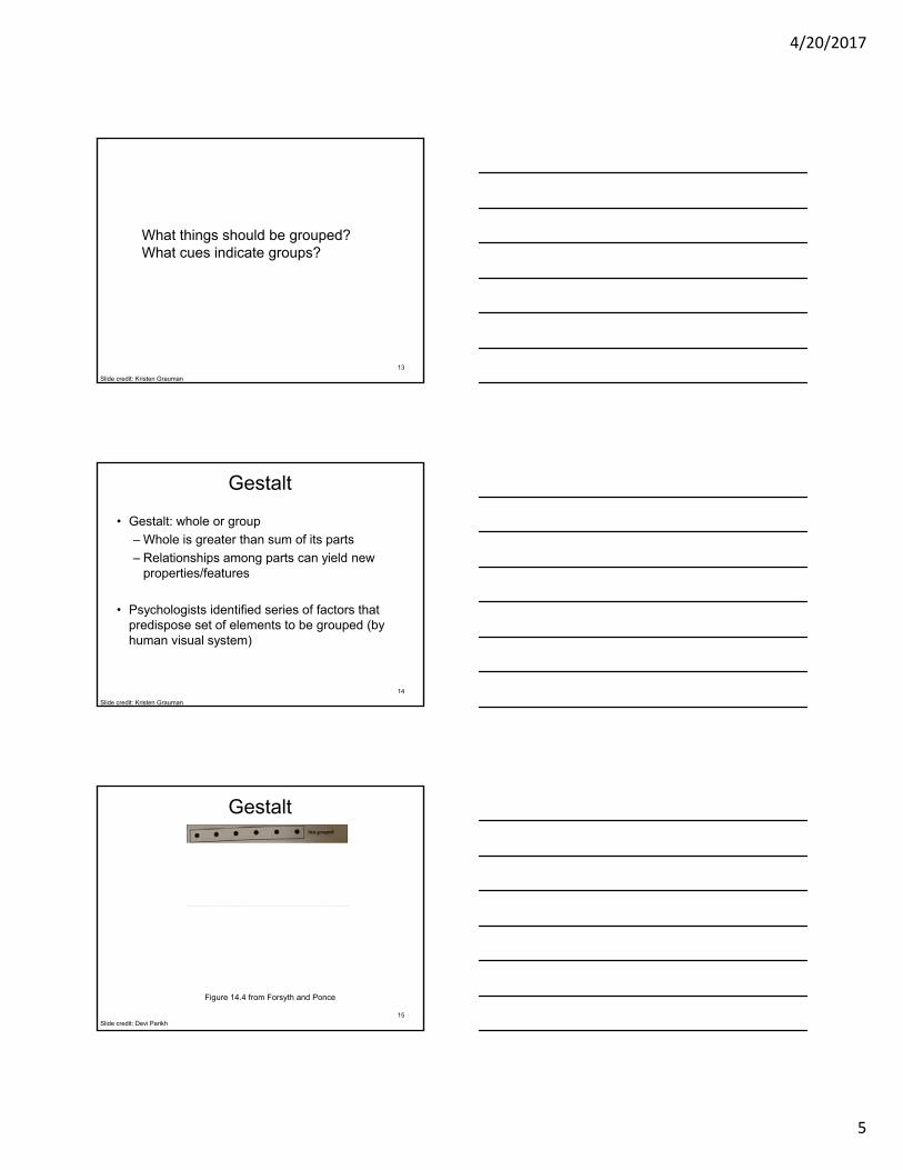
What things should be grouped?What cues indicate groups?

13


Gestalt

• Gestalt: whole or group

– Whole is greater than sum of its parts

– Relationships among parts can yield new properties/features

• Psychologists identified series of factors that predispose set of elements to be grouped (by human visual system)

14


15

Gestalt

Slide credit: Devi Parikh

Figure 14.4 from Forsyth and Ponce

4/20/2017

6

16

Gestalt

Slide credit: Devi Parikh

Similarity

http://chicagoist.com/attachments/chicagoist_alicia/GEESE.jpg, http://wwwdelivery.superstock.com/WI/223/1532/PreviewComp/SuperStock_1532R-0831.jpg

17Kristen Grauman

Symmetry

http://seedmagazine.com/news/2006/10/beauty_is_in_the_processingtim.php

18


4/20/2017

7

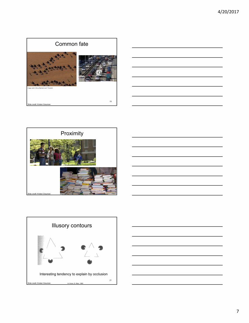
Common fate

Image credit: Arthus-Bertrand (via F. Durand)

19


Proximity

http://www.capital.edu/Resources/Images/outside6_035.jpg

20


Illusory contours

In Vision, D. Marr, 1982

Interesting tendency to explain by occlusion

21


4/20/2017

8

22


Continuity, explanation by occlusion23


D. Forsyth24

4/20/2017

9

25D. Forsyth

Figure-ground

26D. Forsyth

27D. Forsyth

4/20/2017

10

Grouping phenomena in real life

Forsyth & Ponce, Figure 14.728


Grouping phenomena in real life

Forsyth & Ponce, Figure 14.729


Gestalt

• Gestalt: whole or group

– Whole is greater than sum of its parts

– Relationships among parts can yield new properties/features

• Psychologists identified series of factors that predispose set of elements to be grouped (by human visual system)

• Inspiring observations/explanations; challenge remains how to best map to algorithms.

30


4/20/2017

11

Outline







31


The goals of segmentation

Separate image into coherent “objects”image human segmentation

Source: Lana Lazebnik

32

The goals of segmentation

Separate image into coherent “objects”

Group together similar-looking pixels for efficiency of further processing

X. Ren and J. Malik. Learning a classification model for segmentation. ICCV 2003.

“superpixels”

Source: Lana Lazebnik

33

4/20/2017

12

intensityp

ixel

co

un

tinput image

black pixelsgray pixels

white pixels

• These intensities define the three groups.

• We could label every pixel in the image according to which of these primary intensities it is.

• i.e., segment the image based on the intensity feature.

• What if the image isn’t quite so simple?

1 23

Image segmentation: toy example

Kristen Grauman

34

intensity

pix

el c

ou

nt

input image

input imageintensity

pix

el c

ou

nt

Kristen Grauman

35

input imageintensity

pix

el c

ou

nt

• Now how to determine the three main intensities that define our groups?

• We need to cluster.

Kristen Grauman

36

4/20/2017

13

0 190 255

• Goal: choose three “centers” as the representative intensities, and label every pixel according to which of these centers it is nearest to.

• Best cluster centers are those that minimize SSD between all points and their nearest cluster center ci:

1 23

intensity

Kristen Grauman

37

Clustering

• With this objective, it is a “chicken and egg” problem:

– If we knew the cluster centers, we could allocate points to groups by assigning each to its closest center.

– If we knew the group memberships, we could get the centers by computing the mean per group.

Kristen Grauman

38

K-means clustering• Basic idea: randomly initialize the k cluster centers, and

iterate between the two steps we just saw.

1. Randomly initialize the cluster centers, c1, ..., cK

2. Given cluster centers, determine points in each cluster• For each point p, find the closest ci. Put p into cluster i

3. Given points in each cluster, solve for ci

• Set ci to be the mean of points in cluster i

4. If ci have changed, repeat Step 2

Properties• Will always converge to some solution• Can be a “local minimum”

• does not always find the global minimum of objective function:

Source: Steve Seitz

39

4/20/2017

14

Andrew Moore

40

Andrew Moore

41

Andrew Moore

42

4/20/2017

15

Andrew Moore

43

Andrew Moore

44

K-means clustering

• Demo

http://home.dei.polimi.it/matteucc/Clustering/tutorial_html/AppletKM.html

45


4/20/2017

16

K-means: pros and cons

Pros• Simple, fast to compute• Converges to local minimum of

within-cluster squared error

Cons/issues• Setting k?• Sensitive to initial centers• Sensitive to outliers• Detects spherical clusters• Assumes means can be

computed

46Slide credit: Kristen Grauman

An aside: Smoothing out cluster assignments

• Assigning a cluster label per pixel may yield outliers:

1 23

?

original labeled by cluster center’s intensity

• How to ensure they are spatially smooth?

Kristen Grauman

47

Segmentation as clustering

Depending on what we choose as the feature space, we can group pixels in different ways.

Grouping pixels based on intensity similarity

Feature space: intensity value (1-d) 48


4/20/2017

17

K=2

K=3

quantization of the feature space; segmentation label map

49




R=255G=200B=250

R=245G=220B=248

R=15G=189B=2

R=3G=12B=2

R

G

B

Grouping pixels based on color similarity

Feature space: color value (3-d) Kristen Grauman

50



Grouping pixels based on intensity similarity

Clusters based on intensity similarity don’t have to be spatially coherent.

Kristen Grauman

51

4/20/2017

18



X

Grouping pixels based on intensity+position similarity

Y

Intensity

Both regions are black, but if we also include position (x,y), then we could group the two into distinct segments; way to encode both similarity & proximity.Kristen Grauman 52


• Color, brightness, position alone are not enough to distinguish all regions…

53




F24

Grouping pixels based on texture similarity

F2

Feature space: filter bank responses (e.g., 24-d)

F1

…

Filter bank of 24 filters

54


4/20/2017

19

original image

derivative filter responses, squared

statistics to summarize patterns

in small windows

mean d/dxvalue

mean d/dyvalue

Win. #1 4 10

Win.#2 18 7

Win.#9 20 20

…

…

Slide credit: Kristen Grauman55

Recall: texture representation example

Recall: texture representation example

statistics to summarize patterns

in small windows

mean d/dxvalue

mean d/dyvalue

Win. #1 4 10

Win.#2 18 7

Win.#9 20 20

…

…

Dimension 1 (mean d/dx value)

Dim

ensi

on

2 (

mea

n d

/dy

valu

e)

Windows with small gradient in both directions

Windows with primarily vertical edges

Windows with primarily horizontal edges

Both

Kristen Grauman 56

Segmentation with texture features• Find “textons” by clustering vectors of filter bank outputs

• Describe texture in a window based on texton histogram

Malik, Belongie, Leung and Shi. IJCV 2001.

Texton mapImage

Adapted from Lana Lazebnik

Texton index Texton index

Cou

nt

Cou

ntC

ount

Texton index

57

4/20/2017

20

Image segmentation example

Kristen Grauman

58

Color vs. texture

These look very similar in terms of their color distributions (histograms).

How would their texture distributions compare?

Kristen Grauman

59

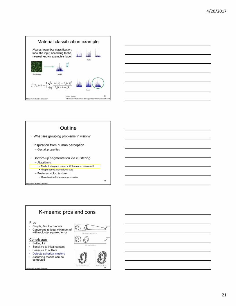
Material classification example

Figure from Varma & Zisserman, IJCV 2005

For an image of a single texture, we can classify it according to its global (image-wide) texton histogram.

60


4/20/2017

21

Manik Varmahttp://www.robots.ox.ac.uk/~vgg/research/texclass/with.html

Material classification example

Nearest neighbor classification: label the input according to the nearest known example’s label.

61


Outline







62


K-means: pros and cons

Pros• Simple, fast to compute• Converges to local minimum of

within-cluster squared error

Cons/issues• Setting k?• Sensitive to initial centers• Sensitive to outliers• Detects spherical clusters• Assuming means can be

computed


4/20/2017

22

• The mean shift algorithm seeks modes or local maxima of density in the feature space

Mean shift algorithm

imageFeature space

(L*u*v* color values)

64


Searchwindow

Center ofmass

Mean Shiftvector

Mean shift

Slide by Y. Ukrainitz & B. Sarel

65

Searchwindow

Center ofmass

Mean Shiftvector

Mean shift


66

4/20/2017

23

Searchwindow

Center ofmass

Mean Shiftvector

Mean shift


67

Searchwindow

Center ofmass

Mean Shiftvector

Mean shift


68

Searchwindow

Center ofmass

Mean Shiftvector

Mean shift


69

4/20/2017

24

Searchwindow

Center ofmass

Mean Shiftvector

Mean shift


70

Searchwindow

Center ofmass

Mean shift


71

• Cluster: all data points in the attraction basin of a mode

• Attraction basin: the region for which all trajectories lead to the same mode

Mean shift clustering


72

4/20/2017

25

• Find features (color, gradients, texture, etc)

• Initialize windows at individual feature points

• Perform mean shift for each window until convergence

• Merge windows that end up near the same “peak” or mode

Mean shift clustering/segmentation

73


Mean shift segmentation results

74


Mean shift

• Pros:– Does not assume shape on clusters

– One parameter choice (window size)

– Generic technique

– Find multiple modes

• Cons:– Selection of window size

– Does not scale well with dimension of feature space

Kristen Grauman

75

4/20/2017

26

Outline







76


q

Images as graphs

Fully-connected graph• node (vertex) for every pixel

• link between every pair of pixels, p,q

• affinity weight wpq for each link (edge)– wpq measures similarity

» similarity is inversely proportional to difference (in color and position…)

p

wpq

w

Source: Steve Seitz77

Measuring affinity

• One possibility:

Small sigma: group only nearby points

Large sigma: group distant points

Kristen Grauman

78

4/20/2017

27

Measuring affinity

σ=.1 σ=.2 σ=1

σ=.2

Data points

Affinity matrices

79


Segmentation by Graph Cuts

Break Graph into Segments• Want to delete links that cross between segments

• Easiest to break links that have low similarity (low weight)– similar pixels should be in the same segments

– dissimilar pixels should be in different segments

w

A B C

Source: Steve Seitz

q

p

wpq

80

Cuts in a graph: Min cut

Link Cut• set of links whose removal makes a graph disconnected

• cost of a cut:

A B

Find minimum cut• gives you a segmentation• fast algorithms exist for doing this

Source: Steve Seitz

BqAp

qpwBAcut,

,),(

81

4/20/2017

28

Minimum cut

• Problem with minimum cut:

Weight of cut proportional to number of edges in the cut; tends to produce small, isolated components.

[Shi & Malik, 2000 PAMI]82


Cuts in a graph: Normalized cut

A B

Normalized Cut• fix bias of Min Cut by normalizing for size of segments:

assoc(A,V) = sum of weights of all edges that touch A

• Ncut value small when we get two clusters with many edges with high weights, and few edges of low weight between them

• Approximate solution for minimizing the Ncut value : generalized eigenvalue problem.

Source: Steve Seitz

),(

),(

),(

),(

VBassoc

BAcut

VAassoc

BAcut

J. Shi and J. Malik, Normalized Cuts and Image Segmentation, CVPR, 1997

83

Example results


4/20/2017

29

Results: Berkeley Segmentation Engine

http://www.cs.berkeley.edu/~fowlkes/BSE/ 85


Normalized cuts: pros and cons

Pros:• Generic framework, flexible to choice of function that

computes weights (“affinities”) between nodes

• Does not require model of the data distribution

Cons:

• Time complexity can be high– Dense, highly connected graphs many affinity computations

– Solving eigenvalue problem

• Preference for balanced partitions

Kristen Grauman

86

Segmentation for efficiency: “superpixels”

[Felzenszwalb and Huttenlocher 2004]

[Hoiem et al. 2005, Mori 2005][Shi and Malik 2001]

4/20/2017

30

Segmentation for object proposals

“Selective Search” [Sande, Uijlings et al. ICCV 2011, IJCV 2013]

[Endres Hoiem ECCV 2010, IJCV 2014]

Motion segmentation

Image Segmentation Motion SegmentationInput sequence

Image Segmentation Motion SegmentationInput sequence

A.Barbu, S.C. Zhu. Generalizing Swendsen-Wang to sampling arbitrary posterior probabilities, IEEE Trans. PAMI, August 2005.

Kristen Grauman

89

Summary• Segmentation to find object boundaries or mid-

level regions, tokens.

• Bottom-up segmentation via clustering– General choices -- features, affinity functions, and

clustering algorithms

• Grouping also useful for quantization, can create new feature summaries– Texton histograms for texture within local region

• Example clustering methods– K-means

– Mean shift

– Graph cut, normalized cuts 90


4/20/2017

31

Coming up

• Fitting

91

Documents

Segmentation and Grouping - Computer Science- UC Davisweb.cs.ucdavis.edu/~yjlee/teaching/ecs174-spring2017/lee_lecture6... · Segmentation and Grouping April 20th, 2017 Yong Jae Lee