Embed Size (px)
Citation preview

SEEPAGE TOWARDS VERTICAL CUTS
By Angel Muleshkov1 and Sunirmal Banerjee,2 Member, ASCE
ABSTRACT: Conformal mapping solutions for two-dimensional steady-state seepage towards vertical excavated faces are presented. Solutions in parametric form are developed for the shape of the free surface and the height of intersection of the free surface and the seepage face. Although the current solution applies strictly to infinite flow domains, an approach to obtain nonparametric solutions for long finite flow domains without much loss of accuracy is also outlined.
INTRODUCTION
A variety of alternative methods have been used for solution of two-dimensional problems involving steady-state seepage within a soil mass. These methods include analytical solution techniques using conformal mapping (Harr 1962; Polubarinova-Kochina 1962), and a number of approximate methods, e.g., flow net technique (Cedergreen 1977); analog methods (Harr 1962; Polubarinova-Kochina 1962); and a few numerical solution techniques—finite difference (Jeppson 1969; Remson et al. 1965), finite element (Desai 1975; Finn 1967), and boundary element (Cruse and Rizzo 1975) methods. In view of the difficulties in developing exact analytical solutions to most seepage problems, it is not surprising that the flow nets and the numerical solution techniques are more popular. However, analytical or closed-form solutions are particularly attractive because of the general nature of these solutions. Furthermore, exact solutions are useful for checking the accuracy of the comprehensive numerical treatments.
In this paper, conformal mapping techniques are used to obtain the solution of a two-dimensional seepage problem. The field problem of interest is steady-state unconfined flow through a homogeneous slope-forming soil mass with a vertical side cut. Although such vertical cuts are commonly encountered along highways and roadways, only approximate solutions are available for this flow problem. The solutions presented in this paper may also be approximately applicable for flow towards retaining walls and long braced excavations if the backfill behind the wall or the bracing system is sufficiently permeable. Furthermore, the solution of the steady seepage problem considered here is also relevant to the long-term stability of these hillside cuts since the available soil strength used to compute safety factors is dependent on the pore pressures (Hodge and Freeze 1977).
•Grad. Stud., Dept. of Appl. Math., Univ. of Washington, Seattle, WA 98195. 2Assoc. Prof., Dept. of Civ. Engrg., Univ. of Washington, Seattle, WA 98195. Note. Discussion open until May 1, 1988. To extend the closing date one month,
a written request must be filed with the ASCE Manager of Journals. The manuscript for this paper was submitted for review and possible publication on April 7, 1986. This paper is part of the Journal of Geotechnical Engineering, Vol. 113, No. 12, December, 1987. ©ASCE, ISSN 0733-9410/87/0012-1419/$01.00. Paper No. 22015.
1419
J. Geotech. Engrg. 1987.113:1419-1431.
Dow
nloa
ded
from
asc
elib
rary
.org
by
Uni
vers
ity o
f N
evad
a, L
as V
egas
on
04/2
1/13
. Cop
yrig
ht A
SCE
. For
per
sona
l use
onl
y; a
ll ri
ghts
res
erve
d.

GOVERNING EQUATION AND BOUNDARY CONDITIONS
Steady flow of groundwater with or without a free surface is described by a velocity potential <f>s, which must, at every point in the field of motion, satisfy Laplace's equation: ,
d24>s d2$s n + ~rrr = 0 dx2 By2 (1)
in which x and y are the horizontal and vertical coordinates respectively, and the velocity potential, <$>s is given by
(2) 4>s = -k(r- + y) + C
where k = coefficient of permeability; p = pressure at any point; 7 = specific weight of the fluid; and C = an arbitrary constant depending on the datum. In the following developments, however, the quantity 4>, which is related to $s by the relationship
< } , = 4>s (3)
will be used. The physical layout of the problem is shown in Fig. 1. Also shown on the same figure are boundaries of the flow domain and the conditions on the boundaries which are discussed later.
In order to make the problem amenable to analysis, a few assumptions are made:
1. The soil is homogeneous, isotropic, and extends to infinite distance to the sides and in depth.
2. The flow is laminar and obeys Darcy's law.
FIG. 1. Physical Layout of Problem
1420
J. Geotech. Engrg. 1987.113:1419-1431.
Dow
nloa
ded
from
asc
elib
rary
.org
by
Uni
vers
ity o
f N
evad
a, L
as V
egas
on
04/2
1/13
. Cop
yrig
ht A
SCE
. For
per
sona
l use
onl
y; a
ll ri
ghts
res
erve
d.

3. Capillary and surface tension effects can be neglected.
The boundary conditions in the physical plane as shown on Fig. 1 are:
1. Along the phreatic surface section of the boundary, 12, the potential and the stream functions can be assumed as
8i> § = y and ^ - = 0 (i.e., y = 0) (4)
on
2. Along the vertical cut 01, 6 (0, y) = y. 3. Along the horizontal boundary 02, 6 (x,0) = 0.
FORMULATION OF PROBLEM
The problem at hand is to find the shape of the phreatic surface line 12, the height, y0 , of the intersection of the phreatic surface and the vertical plane 01 (Fig. 1). Furthermore, the potential function A (x,y) and the stream function >|/ (x,y) at any arbitrary point z (= x + iy) must be found. In order to facilitate the solution of this problem the method of conformal mapping will be used.
It is not easy to find directly a conformal transformation between the image of the domain in the z-plane or the physical plane and that in the to-plane or the complex potential (w = 4> + ty) plane since the flow region is not completely defined on either of these planes. However, for free surface flow problems, it is customary to use two auxiliary functions: (1) Kirchoff's function, W = dz/dio; and (2) Zhukovsky's function W = z - /to; as well as the images of the flow domain in the W and W planes. The Kirchoff's function is the inverse of what is commonly known as the complex velocity function. Either of these functions has been used in the literature (Harr 1962; Polubarinova-Kochina 1962) on this class of problems.
Considering the image of the flow domain in the W-plane (W = $ + FP),
On line 02:
dx .. . 6 = 0, y = Q, i.e., W = - i — (5a)
or
<E> = 0, ¥ < 0 • (5b)
Online 12:
dx + idy dx + idy d, = y v = o, i.c, W = — - = — - ( M
da> dy or
4x0, T=l (6b)
1421
J. Geotech. Engrg. 1987.113:1419-1431.
Dow
nloa
ded
from
asc
elib
rary
.org
by
Uni
vers
ity o
f N
evad
a, L
as V
egas
on
04/2
1/13
. Cop
yrig
ht A
SCE
. For
per
sona
l use
onl
y; a
ll ri
ghts
res
erve
d.

On line 01:
+ = * * = o, ^w = i ^ = TTT- • (7fl)
aq> + idy ay + id\\f
i.e.,
w = J_ y. e = il {lb)
0 — i dy
or
0 1 <D = T= and W = - (7c)
02 + 1 02 + 1 In other words, on line 01, one may write
*F(92 + 1 ) = 1 (8a)
O T X ¥ ( $ + l ) = 1 <•*»>
or *2 + ( ^ - ^ J = Q)2 (8c) Eq. 8(c) is the equation of a semicircle in W-plane. It can also be noted that in the W-plane, the corresponding points are given by: W0 = 0; W1 = i; and W2 = °°. The image of the flow domainjn the W-plane is shown in Fig. 2.
Again, if_Zhukovsky's function, W(W = z - m), is considered, in the W-plane (W = $ + f¥), the flow domain is known. Since 3> = x + \\i and * = y - 4>.
w„=o
FIG. 2. Transformed Domain on W-Plane
1422
J. Geotech. Engrg. 1987.113:1419-1431.
Dow
nloa
ded
from
asc
elib
rary
.org
by
Uni
vers
ity o
f N
evad
a, L
as V
egas
on
04/2
1/13
. Cop
yrig
ht A
SCE
. For
per
sona
l use
onl
y; a
ll ri
ghts
res
erve
d.

On line 02:
4>=.0, y = 0, i.e., $ = x + y and f = 0 (9)
On line 12:
$ = y, v = o, i.e.,$ = x and ¥ = 0 (10)
On line 01:
§ = y, x = 0, i.e., 0 = \|f and <F = 0 (11)
Also,_the corresponding points in the W-plane are given by: W0 = \\>0; W1 = 0; W2 = °°; so that the flow domain in the W-plane can be represented by the half plane shown in Fig. 3.
Considering another analytic function W given by:
_ „ ~ 1 W = <t> + ix¥ = — (12a)
W — i
or
~ 1 dm w=-rz=w (12b)
dm the flow domain can be mapped in the W-plane as shown in Fig. 4. This domain (Fig. 4) can again be represented as a half-plane by the following transformation function, W: W = cos (inW) = cosh (nW) (13)
Fig. 5 shows the corresponding domain in the W-plane. The analytical solution to the problem_js developed in the following
section by relating the two half-planes in W and W.
ANALYTICAL SOLUTION
The relationship between the half planes in W and W is given by:
w-l-7w <14*) or
W = TZW ' (14fo> Substituting Eq. 13 into Eq. 14a, an ordinary differential equation can be obtained as
(. da>\ 2i|/0 c o s r ^ r ^ • (15)
or
-'"£)-'-£ (I6» 1423
J. Geotech. Engrg. 1987.113:1419-1431.
Dow
nloa
ded
from
asc
elib
rary
.org
by
Uni
vers
ity o
f N
evad
a, L
as V
egas
on
04/2
1/13
. Cop
yrig
ht A
SCE
. For
per
sona
l use
onl
y; a
ll ri
ghts
res
erve
d.

4 ^
®ost> Wl=0> W2=«
FIG. 3. Transformed Domain on W-Plane
FIG. 4. Transformed Domain on W-Plane
FIG. 5. Transformed Domain on ll'-Plane
1424
J. Geotech. Engrg. 1987.113:1419-1431.
Dow
nloa
ded
from
asc
elib
rary
.org
by
Uni
vers
ity o
f N
evad
a, L
as V
egas
on
04/2
1/13
. Cop
yrig
ht A
SCE
. For
per
sona
l use
onl
y; a
ll ri
ghts
res
erve
d.

Eqs. 15 and 16 can be recast to obtain
w= .Jl:d^ (i7)
sin \llwj or
W - — f ^ • '(18) sinh [idw,
Defining the complex parameters u and v as
.n da . l2dW = U = - W • • • ( 1 9 )
and recognizing that
i- da = udW = d{uW) - Wdu (20)
Eq. 17 yields
n 2uwn C du -co = - ^ — - 2 V o — 21a 2 1 - cos 2M J 1 - cos 2u
or
in w0 u
2 sin u co = 3 ^ — ( - v|/0 cot u (21ft)
Hence, the solution to the ordinary differential equation is obtained in the parametric form as
a = — (-7^- + cotu\ (22a) ni \sin u J
and z = ia + W = — \ ^ - +cot u\ + -r%- (22b) 7i \sin's u J sm u
Alternatively, the above relations can also be obtained in terms of v as
to = ^ ( —^- + coth v ) (23a) rc \sinh v )
2"fo ( v , __*,. .A Vo 7t \smh i> / sinh v
Equation of the Free-Surface Eqs. 22(a), 22(b), 23(a), and 23(b) provide solutions of the problem in
alternative parametric forms. In order to find the equation of the free
1425
J. Geotech. Engrg. 1987.113:1419-1431.
Dow
nloa
ded
from
asc
elib
rary
.org
by
Uni
vers
ity o
f N
evad
a, L
as V
egas
on
04/2
1/13
. Cop
yrig
ht A
SCE
. For
per
sona
l use
onl
y; a
ll ri
ghts
res
erve
d.

surface, it is necessary to consider either of these two sets of equations and require: $ = y and \\i = 0. From Eqs. 23(a) and 23{b), this gives
x = - ^ ^ • (24) sinh v
^ o f v + \ ( 2 5 )
n \sinhz v J
so that the equation of the free surface, line 12, can be written as
^-= A T ^ - ^ s i n h - [-*• • (26) 2V0 V Vo Vo V d
Furthermore, considering that at point 1, x = 0, y = y0 , and v -> °°,
lim . " = 0 (27a) v^x sinh2 v and
lim(coth v)=l, (276) u-*oo
the height of intersection of the free surface and the vertical face of the cut is obtained as
y0 =— (2»)
n
The equation of the free surface can also be expressed as
— 2* . , _, l—n I 2x J = ^ r s i n h V ^ + V^v (29)
where x = x/y0 ; and y = y/y0 . Fig. 6 shows a plot of the free surface in the x-y plane.
It is possible to approximately check the accuracy of the present solution by comparing the predicted shape of the free surface with that for a similar problem. Polubarinova-Kochina (1962) presents the solution for steady unconfined seepage from infinity towards the vertical seepage face of a dam on impervious base with no tailwater. The dotted line on Fig. 6 shows the free surface of the dam. The excellent agreement between the two free surfaces near the seepage face was obviously expected. Estimation of y0
The equation of the free surface as expressed by Eq. 29 applies, strictly speaking, to the infinite problem in which seepage occurs from infinity towards a vertical cut. Apparently, this solution has no value unless it can be shown that it is applicable to the finite problem for which it. is generally very difficult, if not impossible, to obtain closed-form solutions. However, this kind of a situation often arises in mathematical models of physical phenomena and, for practical purposes, any large distance can be treated as infinitely long, incurring some minor error. For reasons cited earlier, it is extremely difficult to compute this error. An attempt to estimate the
1426
J. Geotech. Engrg. 1987.113:1419-1431.
Dow
nloa
ded
from
asc
elib
rary
.org
by
Uni
vers
ity o
f N
evad
a, L
as V
egas
on
04/2
1/13
. Cop
yrig
ht A
SCE
. For
per
sona
l use
onl
y; a
ll ri
ghts
res
erve
d.
y/y„
Z 4 *'»o°
FIG. 6. Profile of Phreatlc Surface: Straight Line Shows This Study; Dashed Line Illustrates Polubarinova-Kochlna (1962) Study
quantity y0 for a finite problem and the error involved in the solution follows.
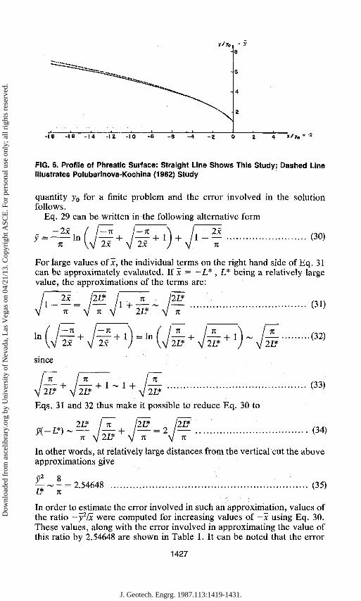
Eq. 29 can be written in the following alternative form
_ _ —2x I / —7i l-n \ I _ 2x „Q.
71 " \ \ / 2x V 2x J V JI
For large values of 3c, the individual terms on the right hand side of Eq. 31 can be approximately evaluated. If x = —L* , L* being a relatively large value, the approximations of the terms are:
J^l-M+z-Jf = z «"> K>/5+>/if+ ')- ta(Vs+7s+i)~^ (32)
since
M+J^~'+M <M» Eqs. 31 and 32 thus make it possible to reduce Eq. 30 to
j ,_ , . ,^/Z+ M_2M (34) 7t V 2L* V 7t V 7t
In other words, at relatively large distances from the vertical cut the above approximations give
v2 8 i - ~ - = 2.54648 (35) L* 7C
In order to estimate the error involved in such an approximation, values of the ratio -y2/x were computed for increasing values of -3c using Eq. 30. These values, along with the error involved in approximating the value of this ratio by 2.54648 are shown in Table 1. It can be noted that the error
1427
J. Geotech. Engrg. 1987.113:1419-1431.
Dow
nloa
ded
from
asc
elib
rary
.org
by
Uni
vers
ity o
f N
evad
a, L
as V
egas
on
04/2
1/13
. Cop
yrig
ht A
SCE
. For
per
sona
l use
onl
y; a
ll ri
ghts
res
erve
d.

TABLE 1. Estimation of Error in Approximation
—x (1)
1.0 2.0 5.0 7.0
10.0 20.0 30.0 50.0 70.0
100.0 200.0 300.0 500.0
1000.0 2000.0
-fix (2)
3.793 3.187 2.808 2.734 2.679 2.613 2.591 2.573 2.565 2.560 2.553 2.551 2.549 2.548 2.547
Errora, % (3)
48.95 25.14 10.28 7.38 5.18 2.60 1.74 1.04 0.75 0.52 0.26 0.17 0.10 0.05 0.02
aError % = -(y2/x/2.54648) x 100 - 100.
decreases very rapidly as -x increases and for relatively large values of —x, this error attains an acceptably low value.
Now, if it is assumed that, at a distance L from the cut, hydrostatic conditions prevail and the height of the free surface to the left of this point is given by H, then the value of y0 can be approximated on the basis of Eq. 35 as
y0
nH2
8L (36)
since y = H/y0 and L* = L/y0 by previous definition. Furthermore, the approximate equation of the free surface valid for large distances away from the cut can be written as
2 8
y +~xyo = 0 7t
(37)
in terms of the actual coordinates of the points on the free surface profile.
Additional Observations It is evident that the unknowns along the other boundaries of the flow
domain can also be evaluated in parametric forms from Eqs. 22(a) and 22(b) or 23(a) and 23(b). First, along the vertical cut 01 where u changes from -ir/2 to °°, defining u as:
u= —- — iX (K varying from 0 to oo) (38)
and noting that
sin u — — cosh X (39)
1428
J. Geotech. Engrg. 1987.113:1419-1431.
Dow
nloa
ded
from
asc
elib
rary
.org
by
Uni
vers
ity o
f N
evad
a, L
as V
egas
on
04/2
1/13
. Cop
yrig
ht A
SCE
. For
per
sona
l use
onl
y; a
ll ri
ghts
res
erve
d.

FIG. 7. Network of $ and i|/ Lines in x-y Space
cos u = — i sinh X (40)
the unknown quantities I|J and y along 01 can be obtained as
¥ cosh2 X
= ^ ( t
(41)
(42) y = ~~^ I tanh X, — — - r , n \ cosh A.
Similarly, along the bottom of cut 02 where u changes from -TT/2 to 0, the unknown quantities are obtained as
W = — I - r i — + cot n 7t \ s u r n
Vo 2Vo x = sin2 (i n \sin2 (x + cot n
(43)
(44)
in which jx = -w (|i varying from TT/2 to 0). Finally, for the internal points in the domain, defining u = s + it, the
unknowns x, y, (j>, and i|> can be expressed in the parametric form as:
— 2s sin 2s sinh It + 2t(l — cos 2s cosh 2t) * = * =
y0 (cosh 2t — cos 2s)2
sinh 2(
cosh It — cos 2s (45)
1429
J. Geotech. Engrg. 1987.113:1419-1431.
Dow
nloa
ded
from
asc
elib
rary
.org
by
Uni
vers
ity o
f N
evad
a, L
as V
egas
on
04/2
1/13
. Cop
yrig
ht A
SCE
. For
per
sona
l use
onl
y; a
ll ri
ghts
res
erve
d.

V .1. y0
•2t sin 2s sinh 2r — 2s(l — cos 2s cosh 2i)
(cosh 2t — cos 2s)2
sin 2s
cosh 2t — cos 2s and
(46)
x y0 L
(2s + 7t)(l - cos 2s cosh It) + 2t sin 2s sinh 2t
(cosh It — cos 2s)2
+ • sin 2s
cosh 2t — cos 2s (47)
- =y_ =
y 0 L
—(2s + n) sin 2s sin 2t + 2t(l — cos 2s cosh 2t)
(cosh 2t — cos 2s)2
sinh 2t
cosh 2t — cos 2s (48)
where y0 = 2^Q/TT = height of free surface at the exit point. Based on Eqs. 45-48, a network of $ = constant and iji = constant lines in the x-y space are presented in Fig. 7.
CONCLUSIONS
Analytical solutions to an important seepage problem have been presented in this paper. The basic approach for the development of the solutions is successive mapping on auxiliary planes. This is a simple but powerful technique compared to the approaches adopted by previous workers to solve similar problems, for instance, the problem of groundwater inflow into a symmetric drainage ditch (Vedernikov 1939) or the problem cited earlier (Polubarinova-Kochina 1962).
Clearly, several restrictive assumptions had to be made in order to avoid complications. The results, nevertheless, should be useful provided the limitations are approximately satisfied.
APPENDIX I. REFERENCES
Cedergreen, Ft. R. (1977). Seepage, drainage and flownets. John Wiley and Sons, New York.
Cruse, T. and Rizzo, F. (1975). "Boundary integral equation methods: computational applications in applied mechanics." ASME Special Publication AMD, 11, June.
Desai, C. S. (1975). "Finite element methods for flow in porous media." Finite elements in fluids, Vol. I., R. H. Gallagher et al., eds., John Wiley and Sons, London, England.
Finn, W. D. L. (1967). "Finite element analysis of seepage through dams." / . Soil Mech. and Found. Div., ASCE, 93(6), 41-48.
Harr, M. E. (1962). Groundwater and seepage. McGraw-Hill Book Co., Inc., New York, N.Y.
Hodge, R. A. L., and Freeze, R. A. (1977). "Groundwater flow systems and slope stability." Can. Geotech. J., 14(4), 466-476.
Jeppson, R. W. (1969). "Free-surface flow through heterogeneous porous
1430
J. Geotech. Engrg. 1987.113:1419-1431.
Dow
nloa
ded
from
asc
elib
rary
.org
by
Uni
vers
ity o
f N
evad
a, L
as V
egas
on
04/2
1/13
. Cop
yrig
ht A
SCE
. For
per
sona
l use
onl
y; a
ll ri
ghts
res
erve
d.

media." J. Hydr. Div., ASCE, 95(1), 363-382. Polubarinova-Kochina, P. Y. (1962). Theory of groundwater movement.
Translated from Russian by J. M. Roger DeWiest, Princeton Univ. Press, Princeton, N.J.
Remson, I., Appel, C. A., and Webster, R. A. (1965). "Groundwater models solved by digital computer." / . Hydr. Div., ASCE, 91(3), 133-147.
Vedernikov, V. V. (1939). Seepage theory and its applications in the field of irrigation and drainage. State Press, Moscow, U.S.S.R.
APPENDIX II. NOTATION
k = coefficient of permeability; n = direction of the normal to boundary; p = pressure at any point; u = complex parameter = s + it; v = complex parameter;
GO = complex potential function; W = Kirchoff's function = dzlda = <I> + n|»; _ W = Zhukovsky's function = z — iw = <F + i§; W = auxiliary function = l/(W —_/); W = auxiliary function = cos(mW); x = physical coordinate variable; y = physical coordinate variable;
y0 = height of free surface at exit point; z — complex coordinate variable; 7 = specific weight of fluid; 9 = real parameter = d\\i/dy; \ = real parameter; (JL = complex parameter = —u\
<i>s = potential function; 4> = reduced potential function; i|/ = stream function; and
i|;0 = stream function value at point 0.
1431
J. Geotech. Engrg. 1987.113:1419-1431.
Dow
nloa
ded
from
asc
elib
rary
.org
by
Uni
vers
ity o
f N
evad
a, L
as V
egas
on
04/2
1/13
. Cop
yrig
ht A
SCE
. For
per
sona
l use
onl
y; a
ll ri
ghts
res
erve
d.