Embed Size (px)
Citation preview

Retrospective Theses and Dissertations Iowa State University Capstones, Theses andDissertations
1983
Sedimentation and self weight consolidation ofdredge spoilTso-Wang LinIowa State University
Follow this and additional works at: https://lib.dr.iastate.edu/rtd
Part of the Civil Engineering Commons
This Dissertation is brought to you for free and open access by the Iowa State University Capstones, Theses and Dissertations at Iowa State UniversityDigital Repository. It has been accepted for inclusion in Retrospective Theses and Dissertations by an authorized administrator of Iowa State UniversityDigital Repository. For more information, please contact [email protected].
Recommended CitationLin, Tso-Wang, "Sedimentation and self weight consolidation of dredge spoil " (1983). Retrospective Theses and Dissertations. 7643.https://lib.dr.iastate.edu/rtd/7643

INFORMATION TO USERS
This reproduction was made from a copy of a document sent to us for microfilming. While the most advanced technology has been used to photograph and reproduce this document, the quality of the reproduction is heavily dependent upon the quality of the material submitted.
The following explanation of techniques is provided to help clarify markings or notations which may appear on this reproduction.
1. The sign or "target" for pages apparently lacking from the document photographed is "Missing Page(s)". If it was possible to obtain the missing page(s) or section, they are spliced into the film along with adjacent pages. This may have necessitated cutting through an image and duplicating adjacent pages to assure complete continuity.
2. When an image on the film is obliterated with a round black mark, it is an indication of either blurred copy because of movement during exposure, duplicate copy, or copyrighted materials that should not have been filmed. For blurred pages, a good image of the page can be found in the adjacent frame. If copyrighted materials were deleted, a target note will appear listing the pages in the adjacent frame.
3. When a map, drawing or chart, etc., is part of the material being photographed, a definite method of "sectioning" the material has been followed. It is customary to begin filming at the upper left hand comer of a large sheet and to continue from left to right in equal sections with small overlaps. If necessary, sectioning is continued again—beginning below the first row and continuing on until complete.
4. For illustrations that cannot be satisfactorily reproduced by xerographic means, photographic prints can be purchased at additional cost and inserted into your xerographic copy. These prints are available upon request from the Dissertations Customer Services Department.
5. Some pages in any document may have indistinct print. In all cases the best available copy has been filmed.
UniversiV Microfilms
International 300 N. Zeeb Road Ann Arbor, Ml 48106


8316153
Lin, Tso-Wang
SEDIMENTATION AND SELF WEIGHT CONSOLIDATION OF DREDGE SPOIL
Iowa State University PH.D. 1983
University Microfilms
I n t6rn Sti O n &l 300 N. Zeeb Road, Ann Arbor, MI 48106


PLEASE NOTE:
In all cases this material has been filmed in the best possible way from the available copy. Problems encountered with this document have been identified here with a check mark V .
1. Glossy photographs or pages ^
2. Colored illustrations, paper or print
3. Photographs with dark background
4. Illustrations are poor copy
5. Pages with black marks, not original copy
6. Print shows through as there is text on both sides of page
7. Indistinct, broken or small print on several pages
8. Print exceeds margin requirements
9. Tightly bound copy with print lost in spine
10. Computer printout pages with indistinct print
11. Page(s) lacking when material received, and not available from school or author.
12. Page(s) seem to be missing in numbering only as text follows.
13. Two pages numbered . Text follows.
14. Curling and wrinkled pages
15. Other
University Microfilms
International


Sedimentation and self weight consolidation
of dredge spoil
by
Tso-Wang Lin
A Dissertation Submitted to the
Graduate Faculty in Partial Fulfillment of the
Requirements for the Degree of
DOCTOR OF PHILOSOPHY
Department : Civil Engineering
Major; Geotechnical Engineering
Approved:
In Charge of Major Work
For the Major Department
For the Graduate College
Iowa State University Ames, Iowa
1983
Signature was redacted for privacy.
Signature was redacted for privacy.
Signature was redacted for privacy.

il
TABLE OF CONTENTS
Page
CHAPTER I. INTRODUCTION 1
Problem Statement 1
Background on Dredge Slurries 2
Literature Review 7
Synthesis of Literature 42
Summary of Literature 49
Objectives of Study 50
CHAPTER II. SETTLING COLUMN TESTS 52
Background of the Area under Study 52
Sediment Properties 54
Test Equipment 57
Test Procedures 58
Test Program 64
CHAPTER III. PRESENTATION AND DISCUSSION OF TEST RESULTS 66
Concentration Profiles 66
Settling Behavior of Interface 70
Critical concentration, c 70 Observed settling behavior 71
Effect of Sampling on Settling Behavior 73
Low initial concentration test 73 High initial concentration test 76 Discussion 76

iii
Page
CHAPTER IV. EVALUATION OF COEFFICIENT OF
CONSOLIDATION, C^ 79 r
Development of Methodology 80
Modified material height, z 80 Models for e^ and 3 ° 81
Slurry height after 100% primary consolidation, 82
Time factor, T, and real time, t 85
Summary of Procedures for Determining C ' 88 r
Sample Calculations 90
CHAPTER V. CONCLUSIONS AND RECOMMENDATIONS 95
Conclusions 95
Recommendations for Future Study 96
REFERENCES 97
ACKNOWLEDGMENTS 99
APPENDIX. TEST RESULTS 100
Results of Zone Settling Tests 101
Results of Flocculent Settling Tests 106

1
CHAPTER I. INTRODUCTION
Problem Statement
In a hydraulic dredging project, the cost for disposing dredge ma
terial contributes a significant portion to the total cost. Dikes,
grading, seeding and easements accounted for 19 to 25 percent of the
total cost of recent western Iowa dredging projects. A nationwide sur
vey showed that the disposal cost generally ranges from 15 to 20 percent
of the total project cost; however, it may be as high as 35 percent if
the dredging size is small (Gallagher and Company, 1978). This cost
probably will go even higher in the future because of the increasing
scarcity of disposal areas. The central issue is then on how to design
an efficient, adequate containment for dredged materials.
Prior to 1970, the dredge spoil containments were sized assuming
that the excavated material will occupy more space in a fill than in-
situ because of the mechanical disturbance of dredging process and the
removal of overburden pressure. Depending upon the texture of sediment
to be dredged, bulking factors of 1.0 to 2.0 were applied to estimate the
required volume of the facility. While this design approach was easy,
uncertainty and dissatisfaction were associated with the use of these
bulking factors because they depended heavily on practical experience
and local conditions. It was observed that by using these factors some
containments have been undersized by as much as 50 percent, and the
others oversized by as much as 100 percent CLacasse et al., 1977).

2
Because materials discharging into the disposal area are in a
suspension of water, a scientific approach to the containment design
problem requires study of the dredged materials' behavior. Sedimenta
tion of particles has been studied for decades in many disciplines other
than geotechnlcal engineering; these include mining and métallurgie
engineering, chemical engineering and sanitary engineering. Some ideas
from these other disciplines have been borrowed by geotechnlcal engineers
and used in their containment designs. Unfortunately, most of the models
proposed in these studies deal only with the "sedimentation" phenomenon
in which the particle weight is solely supported by hydrodynamic forces
and no effective stress exists. When the settling particles eventually
come into contact to form a three-dimensional, interconnected lattice,
effective stresses are developed and sedimentation models fall. Hence,
studies on the settling behavior of suspensions should consider a model
which includes consolidation as well as sedimentation.
Background on Dredge Slurries
Hydraullcally dredged sediments are mixed with ambient water, sucked
into a centrifugal pump, pushed through hundreds or even thousands of
feet of pipe, and discharged into a containment at velocities of about
15 ft/sec. As a result of the mixing with water and the mechanical
disturbance associated with the operations, the volume of the sediments
Increases; however, after sufficient time in the containment, it is pos
sible that the materials will occupy less volume due to the disruption

3
of flocculent structure and consolidation.
Before 1970, the volume of dredge spoil was estimated largely by
rule of thumb of multiplying a bulking factor with the volume of sedi
ments being dredged. Generally, a value of 1.0 was assigned for sand,
1.25 for sandy clay, 1.45 for clay, 1.75 for gravel and rock, and 2.0
for silt as the bulking factor for immediate disposal (Huston, 1970).
Later, the shrinkage of dredge materials due to long term settlement
was considered in design, and a "settlement factor" was usually combined
with the bulking factor to yield a sizing factor for the containment.
According to the practice of several U.S. Army Corps of Engineers dis
tricts, the sizing factor ranges from 0.6 to 1.3 for sand and silt, and
from 1.0 to 2.0 for clay (Laçasse et al., 1977). As for the determina
tion of the detention time required to allow the solids to settle out
of the water, the method employed was the same as the one used in sani
tary engineering; i.e., assuming particles are spherical and settle ac
cording to Stokes' law.
This approach does not account for the fact that dredge materials
will behave differently in different settling environments or under
different operational concentrations. Also, clay particles are flake or
plate shaped rather than spheres, and the material will eventually con
solidate under its own weight. Recognizing the need for more scientific
approaches to the problem of designing dredge spoil containment facili
ties, the U.S. Army Corps of Engineers sponsored research at Waterways
Experiment Station (WES) In Vlcksburg, Mississippi. Between 1975 and

4
1978, this research resulted in over 20 reports covering various aspects
of dredge spoil containments and provided a major advance to state-of-
the-art design. Palermo et al. (1978) summarized the results of the WES
research and provided containment design and management guidelines.
The methodology developed by WES for design of dredge spoil con
tainments requires both a sedimentation test and a consolidation test.
Grab samples from the proposed dredge area are mixed mechanically with
water to the operational concentration and pumped into a settling column.
The mixing and pumping of the slurry is similar to the disturbance that
the sediment experiences in the dredging operation, whereas the behavior
of the slurry in the column simulates conditions in the containment area.
The settlement of the slurry sample in the column is observed periodi
cally, and after sedimentation has finished, samples are taken from slurry
at the bottom of the column for a consolidation test.
To explain the sedimentation behavior, the WES has used the ter
minology from mining engineering (Fitch, 1962) in which the settling
is classified into three categories according to the degree of solid
concentration and interparticle cohesiveness; 1) discrete settling,
2) flocculent settling, and 3) zone settling. In discrete settling,
particles settle individually with constant rate, whereas in flocculent
settling particles agglomerate to form floes and settling rate increases
with time. In zone settling, particles agglomerate further and settle
as a three-dimensional lattice. Because the concentration in most
dredging operations average as high as 145 g/1 (Montgomery, 1978), dis-

5
Crete settling seldom occurs. According to the WES approach, if an
interface between settling solids and the clear, supernatant water is
formed during the test, the phenomenon is said to be in zone settling.
The design criterion is then based on the work by Coe and Clevenger
(1916). If no sharp interface is formed, the slurry is said to be in
flocculent settling, and the design criterion is based upon the approach
proposed by Mclaughlin (1959). Both criteria are used to design con
tainments with sufficient areas and detention times to accommodate con
tinuous dredge disposal activities and remove sufficient suspended
solids. As for the consolidation analysis, the WES approach requires
the sediment samples used in the settling tests also be subjected to con
solidation tests. The test procedure is the same as the conventional con
solidation test except that very low loading stresses are used. The
results are interpreted according to one-dimensional consolidation
theory (Terzaghi, 1925) to estimate the volume and time rate of the
dredge material's consolidation under its own weight.
The development of self weight consolidation theory (Gibson et al.,
1967; Lee and Sills, 1981) provides a refinement for describing the
settlement mechanism and should result in a more rational containment
design approach. The self weight consolidation theory differs from con
ventional one-dimensional consolidation theory in two distinct aspects:
1) no external load is applied to induce settlement; gravitation is the
only driving force and 2) large strains occur in the process. Because
the dredge material always experiences a large amount of strain during

6
consolidation, the assumption that the soil boundaries are fixed, as
In the conventional consolidation theory, does not hold. Thus, the
self weight consolidation theory should predict the material settling
better if used in the WES approach.
Several researchers (Fitch, 1962; Gaudln and Fuerstenau, 1962;
Michaels and Bolger, 1962) observed that in zone settling there was
no jockeying for position by the particles, and the material settled as
a plastic structure. If all the settling particles are locked into a
three-dimensional lattice when zone settling starts, it is reasonable
to conclude that consolidation process also begins at this moment. The
existence of the lattice Implies the existence of effective stresses.
Although experimental proof of the existence of effective stress is quite
difficult, the observed zone settling behavior is similar to that pre
dicted by self weight consolidation theory. This suggests that the
zone settling phenomenon can be described and analyzed according to the
self weight consolidation theory which is in contrast to interpretations
made in previous research. This alternative to the WES approach should
put the settling column tests on a more rational basis and result in
more accurate estimates of the time rate of settlement. Another implica
tion of this hypothesis is that the results of the settling column tests
can be directly used to predict the long term settlement behavior of the
spoil thereby removing the need for conventional consolidation tests.

7
Literature Review
The sedimentation mechanism of a solid water system has been studied
for more than a century since the pioneer work done by Stokes. General
ly, the study has advanced in three major fields: mining and métallurgie
engineering to treat ore pulp, chemical engineering to examine chemical
precipitation, and sanitary engineering to handle sludge or solid waste.
The developments in these disciplines are useful for studying the
settling behavior of the dredge materials; therefore, pertinent litera
ture from these three fields is reviewed and synthesized in the following
paragraphs. The model for flocculent and zone settling deal only with
the sedimentation process and fall to include the consolidation process.
To provide a more complete study, literature on self weight consolida
tion theory is also incorporated in the review.
Coe and Clevenger (1916) were the first to describe the flocculent
settling phenomenon. They assumed that shortly after a settling test
starts, four distinct zones are formed as shown in Figure 1.1. From top
to bottom they are:
A. Zone of clear water
B. Zone of constant concentration which settles at a constant rate
C. Transition zone with concentration decreasing from the bottom (top of zone D) to the top (bottom of zone B)
D. Compression zone in which the floes are brought so close together that they rest directly upon one another, and further elimination of water is a function of time.

8
Figure 1.1 shows the development of these four zones at various stages
of a settling test. Because of the marked concentration difference be
tween A and B, an interface forms, as indicated in Figure 1.1 (II). The
settling of the interface manifests the behavior of zone B until B
diminishes (II, III, IV). After C has disappeared (V), the whole system
undergoes a compression process (called "consolidation" elsewhere in
this study), and eventually stops settling (VI). To explain this mech
anism, Coe and Clevenger (1916) postulated that any layer has a capacity
of discharging solids corresponding to its concentration and settling
velocity. If the layer has a lower discharge capacity than the overly
ing layer, the layer will gain solids and expand its thickness and
eventually dominate the settling behavior of the whole system unless the
supply-discharge trend is changed. Coe and Clevenger prescribed a
series of batch settling tests at various concentrations to obtain the
concentration vs. settling rate relationship from which the solids dis
charging capacity could be calculated, and the design of an ore pulp
thickener is to provide sufficient area to assure that the supply rate of
solids is less than the discharge capacity of the limiting layer. Con
ceptually, the Coe and Clevenger approach is based upon the continuity
equation. In a continuous pulp thickener, a steady state usually occurs,
and different zones maintain constant positions and concentrations. In
this type of thickener, the concept of solids discharging capacity is then
suitable for describing the settling behavior of material. In a thickener
where bottom withdrawal is not possible and concentration varies with

9
time and position, this approach Is not useful.
A mathematical formulation for the thickening mechanism was derived
by Kynch (1952) on the bases that the settling rate, v, of particles
depends on the local concentration c, particles are of same size and
shape, and no flocculatlon occurs. The concentration term, c, was de
fined as the number of particles per unit volume of the dispersion.
Using the continuity equation, Kynch (1952) mathematically showed
that any concentration layer in the settling column can propagate up
wards with a velocity, U, according to U = -ds/dc, where s is the
particle flux, which is defined as the number of particles crossing a
horizontal section per unit area per unit time, or s = cv. If the
settling velocity of particles is a function of concentration, c, only,
the particle flux, s, and therefore the propagating rate U, is also a
function of c only. Because the original concentration is preserved
when the layer propagates through the suspension, the resulting path will
be linear in the height (H) - time (t) coordinates indicating a constant
U (Figure 1.2).
During the settling test, both the particles and the interface are
falling, while the concentration layers are moving upwards. Thus, all
the particles, originally between the Interface and a certain layer,
will fall through that layer when the layer meets the interface. Using
this concept, the settling behavior of the Interface can he predicted.
Kynch (1952) showed that if a settling column test starts out with a
uniform initial concentration, c^, all the upward propagating paths are

10
I II III IV V VI
Figure 1.1. Four settling zones at various stages of a settling test (after Coe and Clevenger, 1916)
w
vc Descending path of the interface
I • Upward, propagating paths of
concentration layers
0 t, Time, t
Figure 1.2. Motion of the interface and concentration layers in a uniform c^ test, according to Kynch theory

11
parallel, and the concentration in the sector AOB of Figure 1.2 is every
where c^, which results in a linear H vs. t plot AB of the falling in
terface. After point B, some higher concentration layer reaches the
Interface, the H vs. t plot then becomes curved, and the descent of the
interface slows. Many researchers (Gaudin et al., 1959; Fitch, 1962),
however, found that the H vs. t plots were strongly curved even at the
beginning of the tests. In the author's study, a linear H vs. t re
lationship occurs only in the initial portion of some tests with low
initial concentration of solids. This deficiency of the Kynch theory
is that the theory works with the particle and layer velocities in a
purely mathematical fashion and neglects physical phenomemon. For ex
ample, in Figure 1.2, the concentration profile at time t^ is idealized
as uniform from the interface, C, to certain depth, D, by the Kynch
approach, whereas in real tests it seldom happens this way (e.g., see
Been and Sills, 1981). Also, depending on the c^, the dredge material
will settle either as floes or as a three-dimensional lattice structure,
but not as individual particles. The applicability of Kynch theory seems
rather doubtful.
Talmage and Fitch (1955) applied Kynch theory to the design of
thickeners. For many years, this procedure has been used for thickener
design in many disciplines. They assumed that a layer of any concentra
tion, Cj^ > c^, is formed instantaneously at the bottom of the column at
the onset of thickening. If the layer reaches the slurry-water inter
face, all solids in the column must have been "sieved" through this layer.

12
According to this argument, a simple material balance equation can be
made, and from a single settling column test result, the c vs. v rela
tionship can then be obtained, and the thickener design is possible.
This approach implies that the settling curve is unique for a given ma
terial; i.e., the settling behavior of high c^ suspension can be obtained
from the later portion of the low c^ test. As will be discussed in
Chapter III, this is not supported by most of the author's tests on lake
sediment. In addition, the concentration of the bottom layer gradually
increases with time due to particle accumulation, instead of being in
stantly achieved.
Talmage and Fitch (1955) also compared the Kynch approach with the
Coe and Clevenger method and found that the two methods agree in the low
concentration range but diverge as concentration increases. This diver
gence, by their argument, was attributed to (Talmage and Fitch, 1955):
The Coe and Clevenger test procedure, however, entails an additional assumption which is not necessarily valid and which is not contained in application of the Kynch analysis. The Coe and Clevenger test procedure ... assumes that the settling characteristics of the floe will be independent of the initial solids concentration in the pulp in which they are
formed.
Therefore, Talmage and Fitch concluded that the Kynch approach is prefer
able. However, Coe and Clevenger prescribed a series of batch settling
tests that result in an initial concentration vs. settling rate relation
ship. On the contrary, the Kynch approach inherits the assumption that

13-14
the settling characteristics of the floe are independent of the initial
concentration because it generates the c vs. v relationship from only one
settling column test result. The assertion and conclusion made by Tal-
mage and Fitch does not seem correct.
Fitch (1962) classified the settling behavior of slurries into four
categories according to the degree of solid concentration and inter-
particle cohesiveness:
A. Clarification, Class 1; is called discrete settling elsewhere. It occurs when no interparticle cohesiveness exists; e.g., sands and gravels, or cohesive particles at extremely low concentrations. Individual particles then settle independently at a constant rate.
B. Clarification, Class 2: is equivalent to the flocculent settling. It occurs when the interparticle agglomeration tendency is high, but the concentration is low. Particles agglomerate to form floes during settling and the settling rate of floes constantly changes.
C. Zone settling; occurs when both the concentration and the interparticle cohesiveness are high. Particles are locked into a plastic structure and subside at the same rate.
D. Compression: i.e., consolidation, occurs when the concentration is so high that the particle weight is no longer supported solely by hydrodynamic force, but by particles underneath as well, following the Coe and Clevenger's definition. The transmission of force through particle contacts in turn puts the solids structure in a compression state and causes settling.
The factors governing the removal of solids were also studied by Fitch.
Using experimental evidence, he found that Kynch's assumption is not com
pletely valid over the entire zone settling regime, and it is not valid
at all in the consolidation regime. Therefore, Fitch (1962) concluded
that the Coe and Clevenger approach seems preferable, although he did it

15
reversely in 1955.
The first nondestructive concentrations measuring device, named
"Transviewer" was constructed by Gaudin and Fuerstenau (1958). This in
strument enables researchers to more precisely measure the concentra
tion at any specific time and location in the settling column test. The
settling behavior of the material can then be studied without extracting
any slurry for concentration measurements. The theory of the device is
that when X-rays are sent through a suspension, part of their intensity
will be lost due to the absorption of the suspension. A counter is used
to pick up the quantity of X-rays transmitted, which theoretically is
related to the density, y, of the suspension as; 1 = 1^ exp(-y^ • Y * d),
where is the mass absorption coefficient which is a function of the
atomic numbers of constituent elements.of the solids, d the diameter of
the column, the reference intensity, I the intensity recorded. If
the energy level of the incident X-rays is kept high and stable enough,
the dependence on atomic number can be neglected. The transmitted X-ray
intensity is then uniquely related to the density of the suspension, and
the concentrations can be easily obtained by the readings recorded by the
counter. A problem concerning the use of the X-ray Transviewer is that
one has to compromise between the travelling speed of the X-ray and the
time constant of the counter in order to obtain a satisfactory measuring
accuracy and spatial resolution combination. Nevertheless, the settling
mass in this case is not disturbed by the insertion of measuring device
or by the removal of solution for concentration measurement as in conven
tional tests.

16
Using the Transviewer, Gaudin and Fuerstenau (1962) observed the
zone settling of a thick suspension as:
The mass is considered to be settling as an aggregate network or as one large floe,.... Furthermore, it seems that this single floe is in a state of compression from the beginning of settling, and that two phases of compression settling exist during sedimentation. The first occurs during the early stage of settling where liquid exudes easily and rapidly from the floe, while the second occurs in the compacting portion of the floe where water escapes more slowly and with much more difficulty.
This phenomenon is identical to what is called "consolidation" in soil
mechanics. Hence, zone settling behavior may be alternatively described
by consolidation theory. As will be discussed later in this chapter,
the variation of escaping rate of fluid (called "permeability" in soil
mechanics) during consolidation can also be included using self weight
consolidation theory. However, Gaudin and Fuerstenau (1962) considered
it as "a filtration phenomenon in which a pulp thickens by filtration of
its contained liquor through the aggregate network of pulp above it."
To model these behaviors, Gaudin and Fuerstenau assumed that the consoli
dating body is mechanically equivalent to a deformable solid containing
numerous vertical tubes and tubules where tubules are conduits with much
smaller diameter than the tubes. Filtration of water through tubes is
completed at an early stage, whereas flow through tubulues continues
indefinitely. Since the size of tubes and tubules varies randomly, a
proper size distribution function must be assigned. For this, they ac
cepted the Schuhmann size distribution. The Schuhmann distribution is

17
described by the equation: y = (x/G)™, where x is the tube size, y the
cumulative fraction of all tubes with size between 0 and x, and G the
maximum tube size. The quantity of fluid flowing through tubes can be
calculated from Poiseuille's law, i.e., if a fluid with viscosity y
flows through a tube having diameter of x, the average flow rate, q, can
be expressed as;
dl 128y
where dp/dl is the pressure gradient in direction 1. Gaudin and
Fuerstenau defined it to be the excess weight of solids per unit area;
i.e., dp/dl = c(G^ - 1)Y^ where c is the concentration expressed in
term of percent by volume, G^ the specific gravity of the solids, and
the unit weight of water. Combining Equation 1.1 with the Schuhmann
distribution then integrating q as a function of x from 0 to G, the whole
size range of tube diameters, a theoretical expression for the filtra
tion rate per unit area can be obtained as:
According to Gaudin and Fuerstenau, the filtration rate of water
can also be determined experimentally by the following steps. From
Transviewer records, the concentration readings at any time and location
can be calculated. It is then possible to draw a family of contour
lines of equal concentration on the height (H) - time (t) coordinates.
Concentration profiles at different time periods are provided from the
Transviewer data. Because no jockeying for position by particles occurs.

18
the descending path for a thin layer above which a certain percentage
of the total solids remain can be traced on the H-t coordinates. By
doing this repeatedly for various percentages, a system of settling
curves can be drawn (Figure 1.3). The settling velocity or, equivalent-
ly, the filtration rate of water, at any point is simply the slope of
the settling curve at that point. The corresponding concentration value
can be read from the iso-concentration lines, and the Q versus c rela
tionship is then established.
The main difficulty in applying the Gaudin and Fuerstenau's model
is that neither m, nor G can be determined independently by these test
results. Gaudin and Fuerstenau (1962) suggested that assuming if m =
1.0 the maximum tube sizes, and therefore the size distributions, under
different concentrations can be obtained by putting the experimental
Q vs. c relationship in the theoretical expression for Q, Equation 1.2.
Using the obtained size distributions, they back calculated the filtra
tion rates, Q, for several pulp concentrations and found that the Qs
agreed well with the experimental ones. Gaudin and Fuersteanu then con
cluded that the Schuhmann function is proper for describing the size
distribution of pores. However, it is the author's opinion that their
conclusion is erroneous; because the experimental Q vs. c relationship
is used to determine the size distribution, and therefore it should not
he reused to check the suitability of the assumed size function. Never
theless, the tube model provides an insight into the settling mechanism.
The implication of this model will be discussed in the synthesis of the

concentration
profile at
t = 0
descending paths of
different increments
concentration profile
at t = t^
t u
X
i J
X
\ %
0 t,
Concentration, g/l Elapsed settling time, t Concentration, g/l
Index» — aJÈ of total solid existing above this line
Figure 1.3. Construction of the descending paths for various increments

20
reviewed literature.
Michaels and Bolger (1962) interpreted the settling mechanism of
clay minerals in terms of particle-particle interactions. Because the
surface characteristics of kaolin and the microstructure it forms in a
suspension have been frequently studied, flocculated kaolin suspensions
were selected for their study. Michaels and Bolger postulated that the
basic units in settling are not particles but floes which have mechanical
strength to resist the viscous shear and maintain their identity during
settling. In a quiescent settling environment, clusters of floes may
agglomerate to form aggregates or even lattice structure depending
on the local clay concentration. According to their test observations,
the aggregates fall individually, roughly in spherical shape in low con
centration suspension. The settling behavior can then be described by
Stokes' law, but the size formed seems to be governed by two counter
acting factors: the collision of aggregates which makes the size grow,
and the viscous shear force in the fluid which breaks down the aggre
gates. Hence, it is a dynamic property, rather than a fundamental floc-
culation phenomenon. Using different mixing methods, they found that
strong mixing usually produces large aggregates and yields higher settling
rate.
Further, Michaels and Bolger tried to model the settling behavior
of a high concentration suspension. They assumed that in the early
settling period the concentration in the upper kaolin laden zone is con
stant, and the zone can be considered as a plug of slurry. The submerged

21
weight of the plug, F^, is
Fp = Al g(Pg - p^) c, (1.3)
where d is the diameter of settling column, Al the length of the plug,
c the concentration in the plug, and F^ is supported by:
(A) resisting force of underlying material:
- I Oy (1-4)
(,B) shear forces at the wall;
F, = ïïdAlT (1.5) b y
(C) force due to pressure gradient which generates the flow through plug:
where and are the compressive and shear strength of the lattice
structure respectively, and dp/dl is the pressure gradient. By Cozeny-
Carman and Poiseuille Equations, the pressure gradient term can be ex
pressed as:
V 1 ^3 . a.7) n
where C is the shape factor of pores, L the tortuosity, s the specific s p
area of pores, and n the porosity. At equilibrium condition, F = F + P &
F + F . An expression for the settling velocity v can thus be obtained, b c

22
Basically, the working mechanism of the above model is similar to
that of the Gaudin and Fuerstenau model, but the additional force terms,
e.g., wall friction and under support, provides a means to account for
the effect of column size and initial slurry height. The model predicts
that the settling rate increases as the slurry height increases. The
settling rate also increases with column size, though the effect is small.
This, however, is contrary to the recent experimental results by Mont
gomery (1978). Montgomery observed that at high concentration in zone
settling, column diameters less than 8 in. resulted in higher settling
velocities than that in larger columns. This indicates that wall fric
tion which retards the settling might be too small to be significant
or that the wall slurry interface may provide less resistant passage
ways for pore water to escape. Because the rate of pore water dissipa
tion is an indication of settling rate in the consolidation regime, the
behavior observed by Montgomery suggests that zone settling is actually
a self weight consolidation phenomenon.
Although some of the aforementioned researchers did notice the
existence of consolidation, their models have no capability of describ
ing it. Recently, this problem was studied by Hayden (1978) of WES.
According to Hayden's argument, a high concentration suspension will
pass through three distinct phases during the process of settling. The
early phase is a period of agglomeration which results from particle
flocculation. If the height of the slurry-supernatant water interface,
H, in this period is plotted against time, t, with H as the ordinate and

23
t as the abscissa, a convex upward relationship will result, indicating
an acceleration in the settling rate. The second phase consists of zone
settling when the interface height varies linearly with time. The
period of constant settling is then followed by a transition period.
After that, the whole slurry enters into the last phase of consolidation.
The settling behavior of the material in the last phase is governed by
one-dimensional consolidation theory.
Hayden also proposed a method for calculating the volume change of
slurry due to self weight consolidation. He assumed that the self weight
consolidation of a layer with initial height H^, and initial void ratio
e will be caused by an effective stress of: o
\ "o (I-S) o
acting on the layer, in Equation (1.8) is the average effective
stress acting at the midheight of the layer. A series of one-dimensional
consolidation tests with a suitable range of loading stresses is per
formed to construct the experimental e-log O curve. The void ratio at
the end of primary consolidation, e^^^, is obtained by interpolating
in e-log a curve. The final slurry height is calculated as;
H ("100 + "'"oV a,) 100 + gg(l - p„) •
where is the percent solid by weight in the original suspension. The
slurry height at the beginning of consolidation, H^, can be obtained
graphically from the settling curve of the interface by extending the

24
tangent to the zone settling portion of the curve to intersect the
tangent to the consolidation portion of the curve. The slurry height
corresponding to the point of intersection is The volume change of
slurry in a disposal site which results from consolidation is then:
AV = A (H^ - , CI. 10)
where A is the area of the dispoal site. According to Hayden, this
volume is the amount of containment capacity regained due to the long
term settlement of the slurry.
Parallel to Hayden's work, Montgomery (1978) of WES studied the
short term settling behaviors of the slurry and proposed a method for
designing containments with sufficient areas and detention times to
accommodate continuous dredge disposal activities and provide sufficient
suspended solids removal. He suggested a settling column with 8 in. in
side diameter and 6 ft. height, to be used for the sedimentation study.
If a sharp interface is formed during the settling test, the slurry is
said to be in zone settling. Although this phenomenon did sometimes
occur in fresh water environment, Montgomery classified it as salt water
settling. Design criterion in this case is based on the concept pro
posed by Coe and Clevenger (1916); i.e., to provide an adequate area so
that the continuous discharging of slurry will not cause any concentra
tion higher than the design concentration. If no sharp interface is ob
served, the slurry is in flocculent settling, and then design approach
is that proposed by Mclaughlin (1959). First, concentration profiles at

25
several time periods after the test has started are plotted according
to the concentration measurement data. Comparing these profiles with the
initial one, a family of curves showing the relationship between percent
solids removal and time at different depths can then be constructed.
Knowing the requirement for returned water quality and the ponding depth,
the detention time can then be obtained by interpolation.
The settling mechanism proposed by the WES studies separates the
consolidation process from the sedimentation process. In reality, how
ever, these two are quite inseparable. Usually, the bigger floes may
have already settled to the bottom of the column and started consolidat
ing, while the smaller floes are still settling in suspension. In addi
tion, this long term settlement analysis inherits all the shortcomings
of the conventional one-dimensional consolidation theory.
Because gravitation force is the sole agent which causes dredge ma
terial to settle, and the strain resulting from this settlement is
generally very large, the volume change behavior of the dredge material
ought to be best described by the self weight consolidation theory. The
equation governing large strain consolidation behavior was formulated by
Gibson et al. (1967). Consolidation parameters are considered to vary
during consolidation, and void ratio, e, is not uniform throughout the
sample thickness. The limitation of fixed soil boundaries as prescribed
in conventional consolidation theory is removed. Because of the moving
boundary, the Lagrangian coordinate system is convenient for describing
the consolidation behavior.

26
Lagrangian coordinate system refers all events back to the initial
t = 0 configuration. Consider a soil layer with a configuration as shown
in Figure 1.4(a) before the consolidation starts. The position of ma
terial points within its domain is described by a space coordinate a.
For example, the datum plane has a position of a = 0, which is assumed
to be fixed. The top boundary is at a = a^. A thin element of soil (A^
B C D ) c a n b e d e f i n e d b y i t s d i s t a n c e , a , f r o m t h e d a t u m p l a n e a n d o o o
its thickness 5^. After some time t, the soil layer has a new configura
tion as shown in Figure 1.4(b) due to consolidation. The top boundary
has moved, and the element of soil occupies a new position (A B CD).
A new position coordinate Ç, called convective coordinate, is then used
to locate the material points [Figure 1.4(b)]. However, inconvenience
arises from the use of ^-coordinate because Ç itself is a function of the
space coordinate, a, and time, t. If the element is labelled according
to its initial position a, which is independent of time, throughout the
consolidation process; e.g., the upper boundary is always considered as
at a = a^ rather than at its current location, C(a^» t), the description
of the system and the introduction of boundary conditions will be great
ly facilitated. This labelling system is called the Lagrangian coordinate
system.
Another coordinate z, called material coordinate or reduced coor
dinate, which labels only the particles, is defined as;
z(a) = ( (1.11)
/Q ^ o

27
where e^ is the void ratio distribution at t = 0, which varies with
position a. Equation 1.11 also implies:
If • ifr o
If the permeability K is assumed to be a function of void ratio only,
i.e., K = K(e), the generalized Darcy's law can be expressed as:
"''f - V * -It where: n = porosity at time t
Vj = velocity of fluid
Vg = velocity of solid
u = excess pore pressure, can be expressed as u = a - a' - u^ where a is the total stress, cj' the effective stress, and u^ the hydrostatic pressure
To work with Equation 1.13, a transformation equation between the con-
vective coordinate Ç and the Lagrangian coordinate a is needed. From
Figure 1.4, the transformation can be expressed in a derivative form as;
i - Hi-o
If both fluid and solids are incompressible, the equilibrium in vertical
direction requires :
II + (e Pg + Pg) = 0 (1.15)

28
where and are the unit weights of pore fluid and solids, respec
tively. To ensure the continuity of fluid flow, the following equation
must be satisfied:
Combining Equations 1.13, 1.15 and 1.16 in terms of z-coordinate, it
results :
P (IS _ 1) JL r_L_l . + A r_K__ . iËl . p^ de 11 + eJ 8z 3z I p^(l + e) de
(1.17)
Equation 1.17 is the general equation governing the large strain con
solidation, which was derived by Gibson et al. (1967).
To obtain an analytical solution, Lee and Sills (1981) assumed
that;
(A) the permeability K increases linearly with void ratio, or
K = p^ K^(l + e) (1.18)
where K is constant. o
(B) the coefficient of consolidation, C^, defined as:
- - K da' (1.19) F pg(l + e) de
is constant throughout the whole consolidation process

29
Equation 1.17 then is reduced to:
S ft - II oz
In order to obtain Equation 1.20, the negative sign in Equation 1.19,
which was not given in Lee and Sills' derivation, is required. The pre
vious assumption implies that da'/de is also constant. Lee and Sills
assumed that a' vs. e relationship to be: a' = A - ae, where A and a
are constant. It should be noticed that both e and a* are functions of
material coordinate z and time t. To solve Equation 1.20, the following
conditions are imposed:
(A) Initial conditions; Prior to self weight consolidation, the concentration, and therefore the void ratio, is uniform throughout the whole depth, and the effective stress is everywhere zero; i.e.,
e(z, 0) = e^
a'(z, 0) = 0 0 z :< z^ (1.21)
where ib the actual material height.
Equation 1.2l results in:
A = Oie^, and
a'(z, t) = aj^e^ - e(.z, t)j (1.22)
(B) Final conditions: After the consolidation has ended, the effective stress is solely due to buoyant weight of
solids because no excess pore pressure exists; i.e.,

and
30
a'(z, 00) = (pg - - z) (1.23)
Pg - Pf e(z, 00) = (z^ - z) =
(1.24)
3(z^ - z)
where 3= (Pg ~ Pj)/^.
Equation 1.24 indicates that after 100 percent primary consolidation the
void ratio will distribute linearly from e^ at the material surface to
e^ - at the base, as shown in Figure 1.5.
(B) Boundary conditions; Since the effective stress is always zero at the material surface, the void ratio at there will then remain unchanged according to Equation 1.22; i.e..
e(z^, t) = (1.25)
In setting column tests or most of the disposal sites for dredge material, bottom drainage is not allowed. The condition at the lower boundary is then;
|H = (cj - a' - u^) = 0
From Equation 1.15, -|^ = - (e + p^). However,
3"li 9"h 95 _ 3z ~ 9Ç 9z ~ ~
3a 3z ) = - Pf(l + e)
Hence,

31
A.
hA
-t
i
«k
Datum plane Q'O
a.
5
*•
Datum plane
Figure 1.4. Lagrangian and convective coordinate: (a) initial configuration, t = 0, (b) configuration at time t
« Z,
I .c
Î C-pz,
Void ratio, e
6(2,0)
Figure 1.5. Assumed initial and final void ratio distributions by Lee and Sills (1981)
32
- u^) = -(ep^ + pg) + Pj(l + e)
Pf - Ps = igr = -"lî
Thus, the boundary condition at the impervious base is:
lî = è<Ps - Pf) = G (1.26)
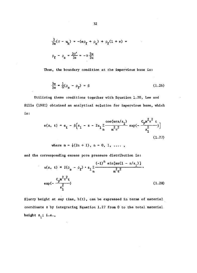
Utilizing these conditions together with Equation 1.20, Lee and
Sills (1981) obtained an analytical solution for impervious base, which
is:
2 2 cos(mTTz/z, ) C_m tt t
i(z, t) = e^ - g^z^ - z - 2z^Z YJ—~ ^~2 )j
(1.27)
n m TT z^
where m = i(2n + 1), n = 0, 1, .... ,
and the corresponding excess pore pressure distribution is;
(-1)^ sinlm7r(l - z/z )]
u(z, t) = 2(p - p ) • z Z 2~2 '
2 2 C m^TT t
exp(- ) (1.28)
=1
Slurry height at any time, h(t), can be expressed in terms of material
coordinate z by integrating Equation 1.27 from 0 to the total material
height z^; i.e.,

33
h(t) =j ^ j^l + e(z, t) j dz
2 00-2 ^(-1)" = (1 + e )z. - igz + 2gz Z - o
^ ^ ^ ^ " m V
2 2 C_m ir t
exp( 2 ) (1.29)
=1
Final slurry height h(a>) is then obtained by letting t-><» in Equation
1.29; i.e.,
h(m) = (1 + e^)z^ - igz^
Since the slurry height prior to consolidation is;
h(0) (1 + e^) dz = (1 + e^) z^,
the degree of self weight consolidation at time t, S(t), can be ex
pressed as: 2 2 9 9 / i\n C m TT t
19,2_ 2gz2zl:|l3 exp(_ -I-,---)
s(t) = h(o) - h(t) S(t) h(0) _ hw
2 2 , nvH TT t
= 1 2—)
® ^ ^1 ci.30)
Cpt Time factor T can be defined as: T = —^ , and M = mïï. Equation 1.30
thus becomes : ^

34
for the impervious base,
S(T) = 1 - 4 E exp(-M^T) (1.31)
" M
where M = nnr = i(2n + 1) . By the same approach except for different
boundary condition at the base, Lee and Sills (1981) also obtained:
for the pervious base,
S'(T) = 1 exp(-4M^T) (1.32)
Equation 1.28 indicates that at the onset of self weight consolida
tion the excess pore pressure distribution generated is triangular. In
classical consolidation theory, the problem concerning triangular initial
excess pore pressure distribution has also been studied by Terzaghi and
Frohlich (1936). In terms of time factor T, their solutions are:
for the pervious base,
S(T) . 1 - a T T \ (1-33)
TT m=l (2m - 1)
and for the pervious base,
s m - 1 4 \ (1.34) TT m=l (2m - 1)
2 where T = c t/h , and c is the coefficient of consolidation. According
V V
to their analysis. Equation 1.34 is also the solution for any linearly
varied initial excess pore pressure distribution with pervious base, in
cluding the uniform one. It should be noticed that the term h in Equation

35
1.33 represents the total thickness of the soil layer, whereas that in
Equation 1.34 only stands for half of the thickness.
Figure 1.6 compares the S(T) vs. /t curves resulting from the clas
sical consolidation theory with those from the self weight consolidation
theory. An important feature is that in the case of the impervious base
both theories predict the same consolidation behavior. This can also be
verified by simplifying Equation 1.33, i.e., letting n = m - 1, and M =
^(2n + 1), Equation 1.33 becomes
32 °° f-D™ / 2 TT^ 1 S(T) = 1 - E % exp (-(2m - 1)^ • ^ T
TT-^ m=l (2m - 1)^ ^ ^ J
1 - 4 Z ^ expf- |(2n + 1) t) n=0 (|(2n + 1)] j I 2 ^
= 1 - 4 Z ^ ^ exp(-M^T) ,
" M
which is identical to Equation 1.31. For the pervious base, however, self
weight consolidation theory predicts a higher consolidation rate than the
classical theory does, though both S(T) vs. /T curves show an initially
linear portion.
In the conventional consolidation test, the Initial pore pressure
distribution is assumed to be uniform throughout the whole sample depth,
and drainage occurs at both top and bottom surfaces. The theoretical
solution for this case is the curve (a) of the pervious base condition,

36
(a) Impervious base
50r b. Self weight
consolidation
theory
a. Classical consolidation
theory
100 0.5 _ 1.0
Vr 1.5
(B) Pervious base
Classical consolidation
b. Se5f \
theory
weight \
consolidatioi\
theory
50
100 0.5
yr 1.0 1.5
Figure 1.6. Comparison of S(T) vs. /t curves for (a) classical consolidation theory, (b) self weight consolidation theory

37
i.e., case (B), in Figure 1.6. The WES study utilizes the test results
to predict the time rate settlement of dredge material, which in essence
is to simulate the consolidation behavior of case (A) by curve (à) of
case (B) in Figure 1.6. An overestimation of settling rate in the early
period of consolidation is expected.
The identical result yielded by these two consolidation theories
in the impervious base case means that the error arising from the
linear a' vs. e and K vs. e assumptions in the self weight consolida
tion theory is probably compensated by the error of assuming small strain
in conventional theory. They are, however, by no means identical. In
fact, the self weight consolidation theory is different from the conven
tional theory by several distinct characteristics: 1) no external load,
2) the variation of soil parameters during consolidation can be accounted
for, 3) large strain, and 4) moving boundaries. In addition, due to the
buoyant effect of the submerged weight of solids, the excess pore pressure
generated initially is always triangular in shape in self weight consolir
dation, whereas in conventional consolidation different external loading
conditions may result in different excess pore pressure distributions.
Furthermore, the self weight consolidation theory deals with the void
ratio distribution and material coordinate. Thus, the slurry height (or
solid boundary) at any time in the consolidation process can be predicated,
e.g., by Equation 1.29, which can serve as a check of how well the theory
can actually model the settlement behavior. The conventional theory,
however, uses pore pressure dissipation as a basis for calculating degree

38
of consolidation and assumes the boundaries to be fixed. It is then
not able to directly predict the slurry height h(t) by solution.
The validity of the Lee and Sills' solution was tested experimental
ly by Been and Sills (1981) using the X-ray Transviewer and pore pres
sure transducers. According to their observations, none of the assump
tions made by Lee and Sills can be experimentally justified. For example,
the permeability, K, is roughly proportional to the void ratio e in a
semilogarithmic fashion, i.e., log K^e, instead of linear fashion as
assumed by Lee and Sills. The relation between e and the effective
stress, a', is well defined when a' is high, but it is poorly defined
when a' is low. In the extreme when a' = 0, the a' vs. e relationship is
not unique because the bulk density at the top of the slurry, where o'
= 0, is observed to be increasing as the consolidation proceeds. Hence,
after 100% primary consolidation the void ratio at the slurry surface
will result in a value e^ < e^, instead of maintaining at e^. In order
to accommodate this real situation to the Lee and Sills' solution. Been
and Sills (1981) assumed that the void ratio difference which occurs at
the slurry surface can be considered as the effect resulting from the
addition of an imaginary overburden layer. The material thickness of this
layer is so defined that the final void ratio still distributes linearly
with material height and has same slope, i.e.,
3(Zo - - e^, (1.35)
where is the material thickness of the imaginary overburden layer

39
(Figure 1.7). The Lee and Sills' solution is still applicable by re
placing for as the total material height, but the excess pore
pressure distribution as expressed in Equation 1.28 needs modification
because there is no excess pore pressure at z = z^ in reality. Thus,
u^(z, t) = u(z, t) - u(z^, t) (1.36)
where 0 z z^, and u^(z, t) is the actual excess pore pressure dis
tribution. Under these circumstances, three soil parameters are required
to be able to describe the self weight consolidation of material; e^,
3 and Cp.
From their tests. Been and Sills (1981) found that both e^ and 3
varied nonlinearly with the initial concentration, although the soils
used were very similar. They argued that the variation was probably
Imaginary
overburden
€(Z,0) •H
Void ratio, e
Figure 1.7. Modified initial and final void ratio distributions by Been and Sills (1981)

40
due to the flocculation and particle segregation in suspensions with low
initial concentrations. However, the behaviors of e^ and 3 were not
examined in detail by them, and both parameters were assumed constant in
their calculations. To determine the coefficient of consolidation, C^,
Been and Sills used three different approaches:
(A) Direct calculation from measured soil properties
Since Darcy's law states that n(v^ - v^) = - Ki, and continuity
equation ensures that v^(l - n) + v^ n = 0, the permeability K can be
expressed as; R = -v^/i. The average fall velocity for an element of
soil, Vg, is obtained by dividing the position change of the soil ele
ment between two concentration profiles by the time interval, and the
pressure gradient, i, can be estimated from the excess pore pressure pro
files constructed by transducer measurements. The corresponding void
ratio, e, for the soil element is calculated from its concentration.
Thus, the K vs. e relationship is obtained. Furthermore, the a' vs. e
relationship is constructed by concentration profiles and pore pressure
measurement, which can generate the da'/de value at any e. Finally, the
coefficient of consolidation is calculated by:
(B) By comparison of pore pressure distributions.
Isochrones of excess pore pressure both from theoretical calculation
and actual measurement are constructed and compared. A time factor, T,
which corresponds to a certain real clock time, t, can be found. The Cj,

41
is then calculated as:
(C) By comparison of settlement curves.
The experimental h(t) vs. t curve is compared with theoretical
S(T) vs. T curve to find the T-t relation. Then, the value is cal
culated as before.
They also compared the results from these three approaches and
found that the value estimated from the settlement curve is much
higher than that given by the other two methods. The difference is ex
pected because both (A) and (B) require an excess pore pressure distribu
tion; whereas (C) doesn't. Been and Sills stated that the value given
by method (A) or (B) is not a good approximation to use.
There is another crucial problem in using the Lee and Sills' solu
tion to interpret the consolidation behavior: how to determine the
starting point of self weight consolidation? Theoretically, the con
solidation process ought to begin at the onset of the development of
the effective stress. However, to experimentally detect the existence
of effective stress is rather difficult because it requires precise
measurements of both density and excess pore pressure profiles. If par
ticles are locked into a three dimensional lattice when zone settling
starts, it is reasonable to conclude that consolidation process also
starts from that moment. It is the author's opinion that Been and Sills
failed to detect the early existence of effective stress, hence their

42
analysis was biased toward the later portion of the self weight consolida
tion.
Synthesis of Literature
This section compares the models reviewed in the preceding section
and studies the similarities and relationships between them so that
the existing models can be better understood and interpreted.
A consolidating soil body can be considered as a deformable solid
containing numerous interconnected pores. Volume change of this body is
then caused by the out flowing of pore water through these passageways.
The seepage velocity v^ of water flowing through a channel can be de
scribed by Poiseuille's law:
V = (C — r^)i (1.38) a s y h
where v^ = average seepage velocity of water through channel
= shape factor
r^ = hydraulic radius of channel section
i = hydraulic gradient
Because the apparent flow velocity v = n v^, and the permeability K =
v/i, the equivalent permeability, K, for the channel is;
Y K = C ^ r ^ n (1 . 3 9 )
s jJ n
where n is the porosity. Taylor (1948) suggested that in the soil sys
tem the hydraulic radius r^ could have a form as:

43
V r = e "T^ (1.40)
^ h where A is the solid surface exposed to flow, and V the volume of
s s
solid. Equation (1.39) thus becomes;
Y 3 V 2
f 3
Therefore, the permeability of the soil should vary linearly with e /I + e
rather than 1 + e (Equation 1.18). In addition, factors like the shape
of the channel and the specific area of solids also influence the permea
bility.
Equation 1.41 also implies that the model using Poiseuille's law is
physically equivalent to the model using Darcy's law as far as the mechan
ism of pore water flow is concerned. For example, the filtration (or
seepage) rate per unit area obtained by the Gaudin and Fuerstenau's model
is:
c(iG - 1)y _
q- %2y % : 2 G
The hydraulic gradient i can be defined as:
i = = c(Gg - 1),
thus the equivalent permeability K for this system is;
Because Gaudin and Fuerstenau (1962) assumed that all the channels are

44
circular in shape, and the tube sizes follow the Schuhmann function,
the expression for permeability K in Equation 1.42 is somewhat different
from the general form, i.e.. Equation 1.41.
In sedimentation, the submerged weight of solids is supported by
hydrodynamic forces. However, once the three-dimensional lattice is
formed, the weight of solids is supported initially by the pressure
generated within pores and later is shared by the soil skeleton and the
pore fluid. At the onset of consolidation, the excess pore pressure dp
generated by a layer of suspension with thickness dl is:
c dV(G - 1)y„ dp = — = 1 = c(G - 1) dl • Y
A A s 'w
where c is the solid concentration expressed in terms of percent by
volume. The resulted pressure gradient is:
^ = c(Gg - 1)Y„, (1-43)
which is exactly the same as that assumed by Gaudin and Fuerstenau
(1962).
From the above discussions, it can be seen that Gaudin and Fuer
stenau' s model is similar to the self weight consolidation model. Never
theless, when the consolidation process starts, and the effective stress
begins to develop. Equation 1.43 no longer holds, and the settling be
havior then can only be described by the self weight consolidation
theory.
By assuming that both permeability K and effective stress a' are

45
linear functions of void ratio e, Lee and Sills (1981) have solved the
self weight consolidation problem. The solutions they obtained for the
impervious base are Equations 1.27 and 1.28. Equation 1.27 indicates
that at slurry surface, where z = z^, the void ratio remains unchanged
throughout the whole consolidation process. However, in reality the
void ratio will reduce from e, to e at the surface. In order to accom-X O
modate this real situation to the Lee and Sills' solutions. Been and
Sills (1981) considered that the void ratio difference at the slurry
surface is due to the effect of adding an imaginary overburden layer
(Figure 1.8). By doing this, the Lee and Sills' solutions are still
applicable if the actual material height is replaced by the modified
material height z^, where z^ = z^ + (e^ - e^)/3. Equation 1.27 then be
comes :
e(y, T') = e. - - z - 2z^ E .
m "iï
exp(-m^7r^T')j (1.44)
for the void ratio distribution, and the corresponding pore pressure
distribution. Equation 1.28, turns out to be;
u(y, T') = 2(Pg - Pg) z^g cos(m^) exp(-m^fr^T'), (1.45)
m IT
2 where y = z/z^ and T' = - t/z^. Equations 1.44 and 1.45 are graphically
shown in Figure 1.8(a) and (b), respectively. Both equations are valid
only for 0 < z < z^.

46
(a) (b)
Imaginary
overburden
0 CQ'
Void ratio, e
0
Normalized u,
Figure 1.8. Modification of Lee and Sills' solution by Been and. Sills (a) void ratio distributions (b) the corresponding excess pore pressure distributions
Either Equation 1.45 or Figure 1.8(b) shows that the excess pore
pressure at z = z^, i.e., the slurry surface, is (p^ - p^) (z^ - z^) at
the beginning of consolidation but reduces to zero after 100 percent of
primary consolidation. In actual settling tests, however, there is no
excess pore pressure existing on the surface at any time. Hence, Been
and Sills further modified Equation 1.45 to be;
u^(z, T') = u(z, T') - u(z^, T') (1.46)
where 0 < zjl z^, or as;

47
2 2 u (y, T') = 2(p -p )z Z T ) miry - cos mirr) 1 s f on ^2^2
(1.47)
in which, r = z^/z^, 0 y r and u^(y, T') is the excess pore pressure
distribution in real soil. Because of the additional modification, the
function used to describe the void ratio distribution at any time, i.e..
Equation 1.44, is not compatible with the function used to describe the
excess pore pressure distribution, i.e.. Equation 1.47. The degree of
consolidation for the modified case, S^(T'), however, should be calcu
lated according to Equation 1.47 because it is close to the real situa
tion. Thus,
S (T') =
\ uL(y, 0)dy - ( u. (y, T')dy -'o -*0
m j-r
^0 j u^(y . 0)dy'
Z| fSinW^r) _ r cos(mUr) ). T i _ exp(-mVT')l)
mV_Li (1.48)
E fsin(mirr) r cos(m'irr)i "I 3 3 " 2 2 j
m ÏÏ m ïï
It is noticed that S^(T') varies with time factor T', as well as r, the
ratio of the real material height z^ to the modified material height z^.
Figure 1.9 shows the plots of S^(T') vs. /T' relationship for different
r values. For r = 1.0, i.e., no imaginary overburden layer exists, the
consolidation behavior is identical to that obtained by Lee and Sills
(1981). As r becomes smaller, the degree of consolidation gets higher
for same T' value, which can be explained as the results of shorter

r value
1.0
Lp.4
Solution ly Lee and Sills (I98I)
0.2 •H
100 0.5 1.0
Figure 1.9. The SmCT') vs. /t' plots for different r values

49
drainage path for water to escape and thicker imaginary overburden layer
exerting on the slurry layer.
Summary of Literature
Prior to 1960, the study of the settling behavior of materials was
primarily based upon the hypotheses that materials fall through fluid
medium as independent particles. No flocculation occurs, and the fall
velocity of particles is a function of local concentration. Intuitive
ly, that was an extension of Stokes' law. Using the concept of material
continuity, simple equations relating concentration with either particle
flux or fall velocity of particles resulted and provided the basis for
thickener designs. These design criteria are not suitable for con
tainment areas because dredge materials always settle as a mass or floes.
In addition, dredge spoil will accumulate and then gradually consolidate
under its own weight instead of being constantly withdrawn from the bottom
as in a thickener.
With the use of the Transviewer, the actual settling behavior of
the material could be examined closely and researchers found that only .
in low concentration suspensions the material settled as individual
floes. Most of the time, it settled as a coherent mass because of
particle agglomeration. The study of zone settling behavior thus
emerged. Generally, the material was modelled as a porous plug contain
ing channels through which water can flow as the material settles. How
ever, these models could not account for the mechanism that as water

50
seeps through the solids, the particles are shoved closer together, and
consoidation occurs. They only resulted in concentration vs. fall
velocity relationships for thickener design. Nevertheless, these
studies provide an insight into the actual settling mechanism.
The WES study combined sedimentation and consolidation in the
settling mechanism, and the approach proposed by the WES researchers
formed a rational basis for dredge spoil containment design. However,
the way WES researchers interpreted the settling column test results
is not satisfactory because the actual settling behavior in the consolida
tion regime bears little resemblance to the theoretical one-dimensional
consolidation curve.
The mathematical formulation for large strain consolidation has
been established. Lee and Sills (1981) applied self weight consolida
tion on the basis of two simple assumptions and their solution which
describes consolidation of soil under its own weight is the most ac
curate one to date. Their solution can also serve as an alternative way
of interpreting the zone settling phenomenon, which may put the settling
column tests on a more rational basis and result in more accurate pre
dictions of the time rate of settlement.
Objectives of Study
The purpose of this study was to examine the settling behavior of
dredge materials for the design of containment areas. Specifically, the
objectives are:

51
(A) to interpret the zone settling test results on the basis of self weight consolidation theory.
(B) to develop a practical approach to evaluate the apparent coefficient of consolidation, Cp, for self
weight consolidation of dredge materials.

52
CHAPTER II. SETTLING COLUMN TESTS
This chapter is essentially a description of the laboratory test
designed for the study of settling behavior of dredge materials, i.e.,
settling column test. Most of the test procedures follow those proposed
by the WES. However, some modification is necessary because the WES
distinction between flocculent settling and zone settling is somewhat
arbitrary and can not suit the study well.
Background of the Area under Study
The sediment samples used in this study are all taken from Lake
Panorama. Lake Panorama, located in Guthrie County, Iowa (Figure 2.1)
is a long narrow impoundment, which was formed by damming a segment of
the Middle Raccoon River in 1970. The watershed above Lake Panorama dam
comprises about 440 square miles, with northeastern two-thirds of it
composed of Wisconsin glacial till and the remaining areas of loess
capped Kansan till (Schaefer, 1980). Because the lake is situated in
an area of high sediment yields and intense cultivation, the problems
associated with lake silting were recognized and studied.
The original capacity of Lake Panorama was calculated to be 19,345
acre-ft (Schaefer, 1980), whereas the hydrographie survey of 1980-81,
conducted by USGS, resulted in a current lake volume of 14,019 acre-
ft (Lin et al., 1981). Comparison of the capacities indicates that
5,326 acre-ft of storage capacity have been lost through sedimentation
in the first 10-year period. Assuming a constant depositional rate of

53
IOWA
miles
Lake Panorama
Panora
Guthrie Center
GUTHRIE COUNTY
Figure 2.1. Location of Lake Panorama (after Schaefer, 198Q)
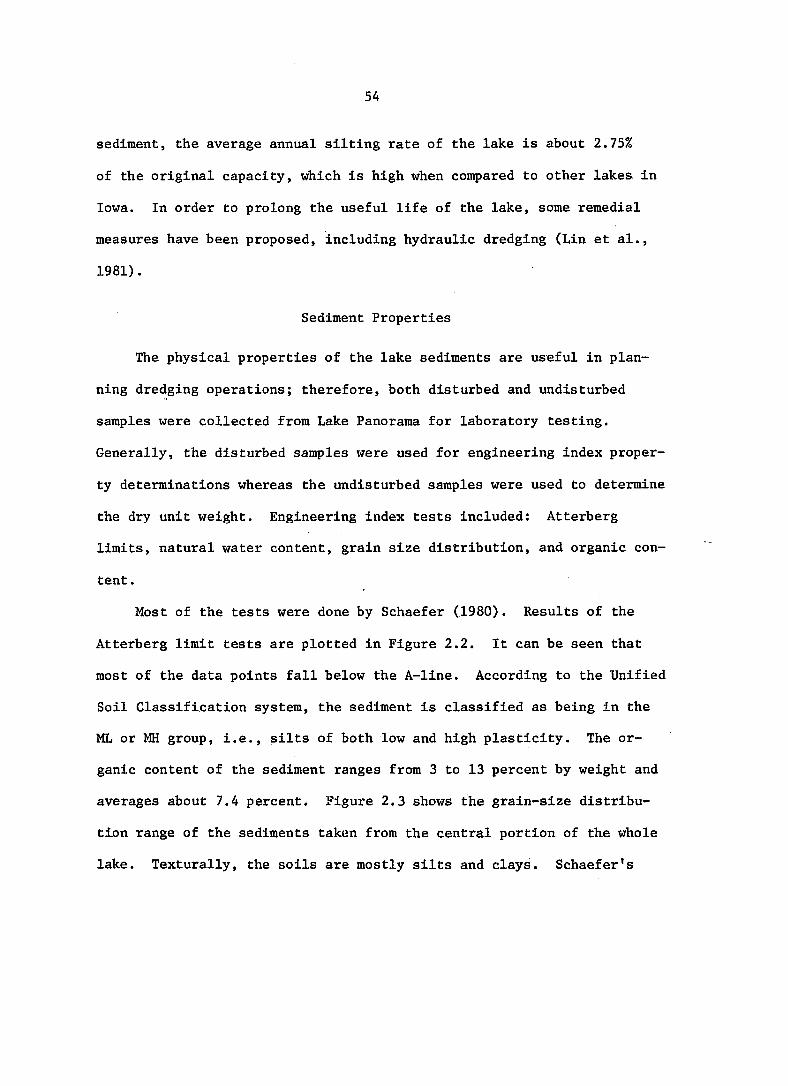
54
sediment, the average annual silting rate of the lake is about 2.75%
of the original capacity, which is high when compared to other lakes in
Iowa. In order to prolong the useful life of the lake, some remedial
measures have been proposed, including hydraulic dredging (Lin et al.,
1981).
Sediment Properties
The physical properties of the lake sediments are useful in plan
ning dredging operations; therefore, both disturbed and undisturbed
samples were collected from Lake Panorama for laboratory testing.
Generally, the disturbed samples were used for engineering index proper
ty determinations whereas the undisturbed samples were used to determine
the dry unit weight. Engineering index tests included; Atterberg
limits, natural water content, grain size distribution, and organic con
tent .
Most of the tests were done by Schaefer (1980). Results of the
Atterberg limit tests are plotted in Figure 2.2. It can be seen that
most of the data points fall below the A-line. According to the Unified
Soil Classification system, the sediment is classified as being in the
ML or MH group, i.e., silts of both low and high plasticity. The or
ganic content of the sediment ranges from 3 to 13 percent by weight and
averages about 7.4 percent. Figure 2.3 shows the grain-size distribu
tion range of the sediments taken from the central portion of the whole
lake. Texturally, the soils are mostly silts and clays. Schaefer's

100
ML
OH or
o OLor ML
60 80
Liquid limit, %
100
• Sample used in
settling test
120 140
Figure 2.2. Classification of sediments from Lake Panorama

Silt Sand Clay Gravel Coo rs• C oo r s * M «d i
100
SO
80
70
60
50
30
o—o Sample used in
settling test 20
10
-3 10 lb
Grain Diameter, mm
Figure 2.3. Grain—size distribution range of sediments from Lake Panorama

57
test on the undisturbed samples resulted in the dry unit weights of the
sediment ranging from 55 pcf to 115 pcf.
The grab samples used in settling column tests were collected from
the proposed dredging site, at about 5.2 miles upstream from Lake Panorama
dam. The sample has the properties of;
Grain-size distribution: 37% clay and 63% silt
Natural water content: 78.9%
Dry unit weight; 50.2 pcf
Organic content: 5.6% by weight
Specific gravity; 2.74
Liquid limit; 59.4
Plasticity index; 24.7
Soil classification: MH
which are comparable to the Schaefer results (Figures 2.2 and 2.3).
Test Equipment
The following equipment is necessary for performing the settling
column test:
(A) Settling column - The WES study suggests that a plexiglass column, at least 8 in. inside diameter, and 6 ft. high should he used. However, in this study, a 5.5 in. diameter column was used because it is readily available. The column should have sample ports at 1 ft. intervals throughout the whole depth.
(^) Portable mixer - used to mix the sediment with water to form a uniform slurry with desired concentration.
(.C) Positive displacement pump - used to discharge slurry into the settling column.

58
CD) Air supply - to keep the particles from settling during the column filling period.
(E) Concentration measurement devices - including hypo
dermic syringes to sample the slurry and a constant
temperature oven to dry out the sample for concentration determination.
Figure 2.4 shows all the equipment except the constant temperature oven.
Test Procedures
Because the slurry discharged into a containment area usually has
a rather high solid concentration, it will behave either as flocculent
settling or as zone settling. In the WES guidelines (Palermo et al.,
1978), the test procedures and design methods are different for these
two types of settling behaviors, but the distinction between flocculent
and zone settling is somewhat arbitrary. Generally, the WES researchers
considered the formation of an interface during the test as evidence
for zone settling (Palermo et al., 1978);
Zone settling where the flocculent suspension forms a lattice structure and settles as a mass, exhibiting a distinct interface during the settling process.
Also, they found (Palermo et al., 1978);
Sedimentation of freshwater sediments at slurry concentration 100 g/1 can generally be characterized by flocculent settling properties. As slurry concentrations are increased, the sedimentation process may be characterized by zone settling properties ... the settling properties of saltwater dredged material can usually be characterized by zone settling tests.

59
Thus, roughly speaking, the freshwater sediments are classified as
flocculent settling materials and the saltwater sediments are considered
as zone settling materials by the WES study, and the containment design
follows the test results accordingly. However, the author's tests on
the freshwater lake sediments show that the interface always forms in
the first hour of the test even at an initial concentration as low as
20 g/1. It is concluded that flocculent settling test alone does not
provide enough information for the sedimentation study of the lake sedi
ments. Hence, both the flocculent and the zone settling tests, pre
scribed by the WES study but with some modification, were performed on
the lake sediments. Generally, procedures for the flocculent settling
test are:
1. Prepare sufficient sediment for the settling test. Calculate the total volume of the column, V. In order to achieve a desired concentration c^, the approximate weight of dry sample needed is c^V, or the amount of wet sediment required is roughly ciV(l + w), where w is the natural water content of the sediment.
2. The sediment is then mixed thoroughly with tap water to
form a uniform slurry (Figure 2.5).
3. Pump the slurry into the settling column, while air is supplied from the bottom of the column to resuspend the falling particles.
4. When thè filling process is finished, draw off samples at each sample port, using hypodermic syringes, for concentration determination. The initial concentration c^ is taken as the average of these concentration readings. After the samples are taken, stop the air supply and begin the settling test. The lineup of the apparatus for this test is shown schematically in Figure 2.6.

60
Figure 2.4. Equipment for performing settling column tests
Figure 2.5. Mixing to obtain a uniform slurry

61
DREDGED MATERIAL SUPPLY
PORTABLE
MIXER
POSITIVE-DISPLACEMENT
PUMP
6'
5 5"
•
MM#
#
SAMPLING PORTS
AIR SUPPLY
SETTLING COLUMN
Figure 2.6. Schematic diagram of apparatus for settling column tests

62
5. At regular time intervals record the height of the interface if it has formed, and then withdraw samples from each sample port to determine the suspended solids concentration (Figure 2.7). Continue the test until the concentration above the interface is less than 1 g/1.
6. The above steps are repeated using different Cj[S ranging from 20 to 200 g/1. The WES researchers recommended that at least two tests should be performed at the proposed operational concentration. If the operational concentration is not available, a cj = 145 g/1 can be used.
The zone settling test is performed according to the following steps;
Steps 1, 2 and 3 are the same as those in flocculent settling test, except determine the c^ by drawing off three samples before the slurry is pumped into the settling column.
4. When the filling process is finished, shut off the air supply and start the test.
5. Observe the settling behavior of the slurry carefully. When a sharp interface between the sediment laden water and the clear supernatant water is formed, record its height and the time elapsed.
6. At regular time intervals record the height of the interface until the height vs. log (time) plot becomes almost linear.
7. Repeat the above procedures for different c^ values. For the purpose of comparison, at least two tests, one on the high Ci side and the other on the low ci side, should be performed using the concentrations identical to those used in flocculent settling test.
The main difference between the two tests is that in flocculent settling
test samples are regularly withdrawn from the column for the determina
tion of the concentration profiles, but not in the zone settling test.

63
Figure,2.7. Sample withdrawal at regular time intervals

64
Test Program
All the tests in this study and their experimental conditions are
listed in Table 2.1. The tests designated by "N" are performed accord
ing to the zone settling test procedures, i.e., no sample withdrawal,
whereas the tests designated by "W" or "L" follow the flocculent settling
test procedures in which samples are regularly taken. Tests L-1 and
L-2 are low initial concentration tests. It can be seen that the ini
tial concentration used in test W-1, W-2 and W-4 are very close to those
for N-1, N-2 and N-4, respectively. The purpose is to examine the ef
fect of sampling on the settling behavior of the slurry.

Table 2.1 Details of test conditions
Initial concentration Initial height Duration Type of test Experiment g/1 in. hours
N-1 75.3 70.75 125.0
Zone N-2 101.0 70.75 54.4
settling N-3 147.0 70.75 56.0
test N-4 191.5 71.00 53.0
N-5 226.5 71.25 70.3
W-1 76.0 70.5 45.3
W-2 99.1 70.5 119.2 Flocculent /
W-3 125.0 70.5 141.0 settling
W-4 190.0 70.5 53.3 test
L-1 20.0 70.5 72.2
L-2 30.0 70.5 124.3

66
CHAPTER III. PRESENTATION AND
DISCUSSION OF TEST RESULTS
The settling behavior of the slurry under the condition of no sample
extraction is characterized by observing the height of the interface at
various times in a zone settling test. Alternately, the concentration
profiles of the slurry at various times are obtained by performing the
flocculent settling test procedures. The slurry height at various times
is also observed in flocculent settling test. This chapter describes
the observations in both zone settling and flocculent settling tests and
discusses the implications of the test results. The settling curves and
concentration plots resulting from both types of settling tests are sum
marized in the Appendix.
Concentration Profiles
To precisely and continuously measure the solid concentration along
the settling column without disturbing the slurry requires elaborate
testing equipment like the X-ray Transviewer. In this study, however,
a crude method is employed, i.e., extracting samples from the settling
column for concentration determination. Hence, the results are used
only for qualitative analysis.
Figure 3.1 shows the concentration variation at various time in
tervals for a slurry with an initial concentration of 99.1 g/1 and results
are typical of most of the flocculent settling tests. The exceptions are

30 min. Average c.= 99.1 g/l
c •H
I •H
w
20
10
0 200 100 300 Concentration, g/l
Figure 3.1. Typical concentration profiles resulting from settling test

68
tests with very low Initial concentrations. Initially, the concentration
is nearly uniform throughout the column, shown by the 0 mln. profile,
indicating that the air supply at the column base is able to prevent
particles from accumulating during the column filling period. After the
test begins, the suspension in the upper portion starts to settle and
becomes less concentrated than the initial concentration, c^. Tlie super
natant water left above the falling suspension is turbid partly because
the finer particles still suspend in water and partly as the result of
the upward moving particle flux. No interface exists at this time.
The jostling particle flux will eventually quiet down, the supernatant
water clears up, and a sharp interface forms. From then on, all the
particles seem to be locked into a three-dimensional lattice and settle
as a mass.
At the column base, however, a high concentration zone is formed
shortly after the test starts, which shows a high vertical concentration
gradient. This zone results from the accumulation and consolidation of
the fast settling floes. As the test progresses, this zone increases
in both thickness and concentration and finally meets the falling inter
face .
The test with low initial concentration, however, displays concen
tration profiles quite different from those discussed above. Figure
3.2 shows the results of a test in which c^ is equal to 30 g/1. The
uniform concentration seems to decrease quickly while, at the column
base, the high concentration zone forms. Then, the interface forms, and
particles settle as a mass.

70
60
50
•S 40
I ^ 30
20
10
V
1
1 j
0 min. Average 30 g/l
1
I 1 ) \30 min.
i
! 60 min.
-
.1 1 -50 100
Concentration, g/l
150
Figure 3.2. Concentration profiles for very low c. test

70
Settling Behavior of Interface
Critical concentration, c^
The zone settling test with low initial concentration, c^, reveals
that a relatively long period of time is required to form the interface.
The time required to form the interface is inversely proportional to the
Cj^ used. For example, Table 3.1 shows that the time required for the in
terface to form is 80 min. in test N-1 (c^ = 75.3 g/1) but 10 min. in
test N-3 (c^ = 147 g/1). When c^ is higher than 147 g/1, the interface
forms immediately after the test starts (N-4 and N-5). If self weight
consolidation begins after the interface is formed, it is concluded that
a critical concentration, c^, exists in the settling process such that
the slurry begins to consolidate under its own weight when its concentra
tion is equal to or higher than c^. The value of c^ depends on the
Table 3.1. Calculation of critical concentration c c
c. H. t * H b
c Test
i X c c c
g/1 in. min. in. g/1
N-1 75.3 70.75 80 34.95 152.4
N-2 101.0 70.75 70 49.40 144.7
N-3 147.0 70.75 10 69.60 149.4
N-4 191.5 71.0
N-5 226.5 71.25
^Time required for the interface to form.
^Critical concentration, is calculated according to c^ = c^H^/H^.

71
material being tested and the settling environment, e.g., column size
and electrolyte concentration in the suspending medium.
The approximate value of c^ for a low c^ test can be obtained by
the following steps. First, observe the slurry height, when the
sharp interface is formed. Because the test starts with an initial con
centration c^ and initial height H^, the average concentration of the
slurry is when the slurry height is Thus, the critical
concentration c^ can be approximately taken as c^H^/H^. Table 3.1 sum
marizes the calculation of c s for N-1, N-2 and N-3. The three c c c
values are close and average about 148 g/1.
Observed settling behavior
Figure 3.3 shows the settling behaviors of tests N-1, N-3 and N-5,
in which the observed slurry height, H, is plotted versus square root
of time, /t. In general, the lower the initial concentration, the
higher the settling rate. If the test starts with a high c^ (N-5), the
interface immediately forms, and the settling curve shows an early con
vex upward portion. However, in the low c^ test (N-1), a period of
time has elapsed before the interface forms, and the early convex por
tion is flattened. After passing the early settling period, all curves
show a concave upward transition period and then become almost linear
with /t.
When Figure 3.3 is compared to the theoretical S(T) vs. /T curves
for the modified self weight consolidation theory, i.e., Figure 1.9,
it is observed that the shape of the settling curve resulting from the

I 0) s:
fH to
10
^ X \ ^ V Q I Q \ ; \ \ t Q H
% V R 4 \ \ \ Q \
9 \ \ \ V \ % \ D 1 \ \ o \ ; \ ^ 1 \ \ b o— ' Test N—5 » c^= 226.5 g/l
" ~—o _____Te8t N-3, 147.0 g/l
t 1 1
"— Test N-1,
' I '
Ci=75.3 g/l
«
0 10 20 30 4o
^Time,
50 60 70 80 90
ro
mm.
Figure 3.3. Comparison of settling behaviors of slurry at different initial concentrations

73
high test is similar to the theoretical curve with high r value,
whereas the experimental curve from the low c^ test is similar to the
theoretical curve having low r value. This observation supports the
hypothesis that the settling behavior of the slurry after the interface
has formed can be described by the self weight consolidation theory.
If the slurry height in Figure 3.3 is plotted versus time, t.
Figure 3.4 results. It is observed that the results of tests N-3 and
N-5 do not show linear settling behavior in the beginning portion of
the test, which is in contrast to what Kynch (1952) expected. Linear
settling behavior only occurs in the early period of the c^ = 75.3
g/1 (N-1) test before the interface has formed. Hence, Kynch theory is
not capable of describing the zone settling behavior of the slurry.
From Figure 3.4, it is also observed that the settling behavior of
the slurry depends very much on the initial concentration used, and it
is impossible to obtain the settling behavior of the high c^ test from
the later portion of the low c^ test because these curves are quite dif
ferent in shape. Thus, the approach proposed by Talmage and Fitch (1955)
does not seem correct.
Effect of Sampling on Settling Behavior
Low initial concentration test
The settling curves resulting from two c^ = 75 g/1 tests, one with
sample extraction (test W-1) and the other without (test N-1), are com
pared in Figure 3.5. Both curves show that a period of time has elapsed

Test N-5, c.= 226.5 g/l c •H
Test N-3. c.= 147.0 g/l iH CO
20
Test N-1, c.= 75-3 g/l
10 10 20
Figure 3.4. Comparison of settling behaviors of slurry at different initial concentrations

-p s 5
a
70
60
50
40
30
20
10
P \
4
i k
SEDIMENTATION
^^ Test with sample extraction (W-l)
® 0 Test without sample extraction (N-l)
SEIP WEIGHT CONSOLIDATION
40 50
VHmë7~riiïn7
60 70 80
Figure 3.5. Comparison of tests with and without sample extraction (c^ 75 g/1)
90
Ln

76
before the interface is formed. The settling behavior of the slurry in
this period is obtained by observing the falling of the dark zone formed
due to the concentration difference between the slurry and the turbid
supernatant water. As can be seen in Figure 3.5, sample withdrawal does
not produce a discernible effect on the settling behavior in this early
period but slightly shortens the time required to form the interface,
t^. Due to the shorter t^, the slurry in test W-1 lags behind in
settling distance. However, after the interface has formed, sample ex
traction seems to accelerate the settling of the slurry because the
slurry height of test W-1 eventually catches up to that of test N-1.
This behavior is also observed in the comparison of tests N-2 and W-2,
both having c^ = 100 g/1.
High initial concentration test
Tests N-4 and W-4, both with initial concentration about 190 g/1,
are compared in Figure 3.6. Because the initial concentration is higher
than the critical concentration (estimated to be about 148 g/1 in pre
vious section), the interface forms immediately after the test starts.
It is noticed that the slurry in W-4, the test with regular sample ex
traction, shows a much higher settling rate than that in test without
sample withdrawal, i.e., test N-4, indicating sample extraction increases
the settling rate after the interface has formed.
Discussion
The above phenomena can be explained using a sedimentation consolida
tion mechanism. After the interface has formed, the system is said to

A—A Test with sample extraction (W-4)
0 Test without sample extraction (N-4)
c •H
+» S
20
10 40 60 80 0 10 20 90 30 70
jTime, rain.
Figure 3.6. Comparison of tests with and without sample extraction (c. = 190 g/1)

78
be in consolidation regime, where excess pore pressure has built up.
The insertion of hypodermic needles at various depths creates many
artificial passageways for pore fluid to escape, and the sample with
drawal aids the dissipation of excess pore pressure. Both accelerate
the consolidation rate. However, before the interface forms, particles
are in sedimentation, and no excess pore pressure exists. Thus, the
sampling procedures cause only a minor influence on settling behavior.
This explanation provides indirect evidence that zone settling can be
considered as a self weight consolidation mechanism.

79
CHAPTER IV. EVALUATION OF COEFFICIENT
OF CONSOLIDATION, C_ r
In conventional consolidation theory, the prediction of time rate
of settlement of a consolidating soil layer requires the determination
of the coefficient of consolidation, c^, for that soil. The coefficient
of consolidation is a soil parameter which relates the theoretical time
factor, T, to real time and the thickness of the soil layer, and thus
applies the consolidation theory to prediction of the behavior of a
specific soil layer. In self weight consolidation theory, the coef
ficient of consolidation is designated as C , but it is still the key F
parameter for describing the settling behavior of a slurry consolidating
under its own weight.
As described in the previous chapter, the study by Been and Sills
(1981) shows that the coefficient of consolidation can be measured using
elaborate instrumentation in a settling column test. However, the
equipment they used is costly, and the test procedures are time con
suming and required skilled personnel to perform them. Hence, this ap
proach is not suitable for conventional engineering design.
In this chapter, a simplified approach to evaluate the apparent
coefficient of consolidation, C^, is developed based upon the modified
self weight consolidation theory by Been and Sills (1981). Because the
Cp calculation in this approach requires only the zone settling test
results, density and pore pressure measuring devices are not needed.

80
Development of Methodology
The coefficient of consolidation, C^, is calculated according to
Equation 1.37 as:
T z S = -T^ (1-37)
where z = the modified material height to account for the void ratio change at the slurry surface
T = theoretical time factor of certain percentage of consolidation
t = real clock time corresponding to that percentage of consolidation
Usually, some curve fitting method is employed to relate the theoretical
time factor T and the real time t. In this study, the square root of
time fitting method is used. It should be noticed that the basic as
sumption for the curve fitting method is that the observed settling
curves are similar in shape to the theoretical ones. Thus, it is neces
sary to check the validity of this assumption when the curve fitting
method is applied. The following paragraphs describe the method for
obtaining the necessary terms in Equation 1.37 to evaluate the C_. r
Modified material height,
From Equation 1.35, the modified material height z^ can be expressed
as :
z = z, + Ce. - e )/3 o 1 1 o
(4.1)

81
where = actual material height, which can be calculated as ;
3 = slope of final (i.e., after 100 percent primary consolidation) void ratio distribution
e. = initial void ratio at the onset of self weight consolida-^ tion
e^ = final void ratio at the slurry surface
For clarification of each term, refer to Figure 1.7. The quantities
and e^ are related to the initial test conditions; hence, they can
easily be obtained. Thfe parameters e^ and 3, however, are used to de
scribe the final void distribution and required more calculations.
Models for e^ and 3 Been and Sills (1981) plotted e^ and 3
versus the initial density of the slurry. Nevertheless, it seems more
appropriate to relate e^ and 3 to the concentration at which self weight
consolidation starts. All the settling column tests with initial con
centration, c^, lower than the critical concentration, c^, will start
the consolidation process at the critical concentration c^ and thus are
assumed to result in only one set of e^ and 3 after 100 percent primary
consolidation. Any test with c^ higher than c^ will result in a set
of e^ and 3 values corresponding to its initial concentration because
consolidation begins immediately after the test starts. Conceptually,
there exists a limiting concentration, c^, beyond which a normally con
solidated soil stratum is formed, and no self weight consolidation occurs.
Thus, if c. > c , the uniform initial concentration profile is maintained i — m

82
because of no self weight consolidation, or 3 • 0 and Between
the two limits c and c , e and 3 are assumed to be functions of c. m c o 1
only. Many simple functions satisfying the conditions at the limiting
concentration c were evaluated, but it was found that only the loga-in
rithmic function can be successfully applied. Thus, the models for
describing the variation of e and 3 between c and c are assumed to o m c
be:
e = e + k„ ln(c /c. ) o m 2 mi
where e = void ratio corresponding to the limiting concentration, c , can be calculated as: m
'm • • W - 1
= proportional constant having a unit of 1/length in order to satisfy the dimension equality in Equation 1.35
kg = dimensionless constant
Slurry height after 100% primary consolidation, The de
termination of the critical concentration c has been discussed in c
Chapter III, but to obtain the parameters c^, k^^ and k^ in Equation 4.2
it is necessary to introduce a quantity which can be measured in the
settling column test and relates c with k and k„. For this, the slur-m i z
ry height after 100 percent self weight consolidation, is chosen.
Theoretically, is related to e^ and 3 as:

83
Hj^OO = j ^ (1 + + 3z)dz = (1 + (4.3)
Combining Equation 4.2 with 4.3, the expression for Hq^qq becomes:
"lOO " [kz'l" "m - 1" =!> + -m
Jk (In c - In c.) z (4.4) 1 m il
The quantity for a zone settling test can be estimated from
the settling curve. First, the observed slurry height is plotted
against /T. Usually, the later portion of the curve becomes approxim
ately horizontal; therefore, the slurry height corresponding to this
horizontal portion is taken as For example, Figure 4.1 shows the
slurry height vs. /t~curve for test N-3(c^ = 147 g/1), and the H^^qq
is estimated to be about 18.8 in.
In order to solve the three unknown quantities c^, k^^ and kg in
Equation 4.4, at least three zone settling tests on the same material
should be performed. The e^ and 3 values for any specific test are then
obtained by Equation 4.2, and the corresponding is calculated by Equa
tion 4.1.

Test N-3, c^= 147.0 g/l
20 = 18.8
100
10 10 20
Figure 4.1. Estimation of the slurry height after 100% primary consolidation,

85
Time factor, T, and real time, t
The degree of consolidation, S^^T), for the modified self weight
consolidation theory is given by Equation 1.48 and can be simplified as:
E j - £-52|_to 1 . n . 1
• ",fslnMr" r cos Mr]
2 where T = C„ • t/z
r O
M = mil" = i(2n + l)Tr n = 0, 1, 2 ....
r -
Thus, S (T) is a function of both time factor T and the ratio r. For a m
specific test, and z^, and therefore r, can be obtained by the ap
proach discussed in the previous section. Knowing the value of r, a
theoretical S^(T) vs. /T curve corresponding to this test results.
To illustrate /t - fitting method, the results of test N-3 are
used as an example. The observed slurry height for this test is plotted
against /t in Figure 4.2. Because r value for this test is about 0.22,
the theoretical S (T) vs. /T curve for r = 0.22 is constructed from m
Equation 4.5 as in Figure 4.3. The following procedures are performed
to obtain both T and t for 90 percent self weight consolidation of the
slurry:
1. On the theoretical curve, e.g., Figure 4.3, locate the inflection point, B, and draw a tangent line through B to intersect the 0 percent horizontal line at point, A.
2. Find the 90 percent consolidation point, P, on the
theoretical curve. The time factor for 90 percent

Test N-3, 147.0 g/l
ton= (91.5-3.2)^= 7797 min.
•H
20
10 20
yTime, min
Figure 4.2. /t-fitting method applied on the settling curve of test N-3(r - 0.22)

0
va lue as
.22
Tgo = (0.657) - 0.432
PI Slope ratio R =-^= 3.94
0.5
F 1.0 1.5
Figure 4.3. /t-fitting method applied on the theoretical S^^T) vs vf curve with r - 0.22
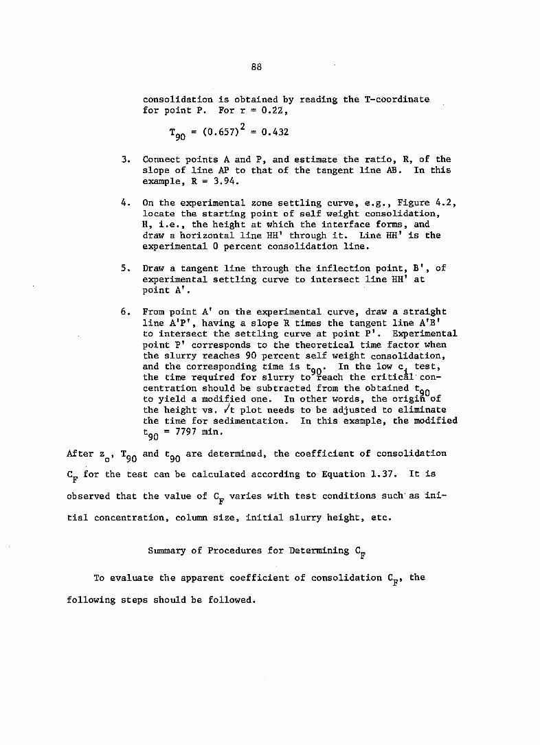
88
consolidation is obtained by reading the T-coordinate for point P. For r = 0.22,
Tgg = (0.657)2 = 0.432
3. Connect points A and P, and estimate the ratio, R, of the slope of line AP to that of the tangent line AB. In this example, R = 3.94.
4. On the experimental zone settling curve, e.g.. Figure 4.2, locate the starting point of self weight consolidation, H, i.e., the height at which the interface forms, and draw a horizontal line HH' through it. Line HH' is the experimental 0 percent consolidation line.
5. Draw a tangent line through the inflection point, B', of experimental settling curve to intersect line HH' at point A'.
6. From point A' on the experimental curve, draw a straight line A'P', having a slope R times the tangent line A'B' to intersect the settling curve at point P'. Experimental point P' corresponds to the theoretical time factor when the slurry reaches 90 percent self weight consolidation, and the corresponding time is t_Q. In the low c^ test, the time required for slurry to reach the critical concentration should be subtracted from the obtained tg^ to yield a modified one. In other words, the origin of the height vs. /t plot needs to be adjusted to eliminate the time for sedimentation. In this example, the modified tgg = 7797 min.
After z^, Tgg and tg^ are determined, the coefficient of consolidation
C„ for the test can be calculated according to Equation 1.37. It is r
observed that the value of varies with test conditions such as ini
tial concentration, column size, initial slurry height, etc.
Summary of Procedures for Determining
To evaluate the apparent coefficient of consolidation C^, the
following steps should be followed.

89
Perform zone settling tests at different selected initial concentrations, ranging from 20 g/1 to 200 g/1. At least two low c. tests are needed to obtain the critical concentration Cg, and additional three tests with Ci > c„ are required to determine the three constants c , 1 • j i m
and kg.
Plot the observed slurry height, H, versus /t curves separately for each test.
Estimate the quantity H^oO each test from the corresponding H vs. /t curve.
Establish three experimental simultaneous, equations according to Equation 4.4 using three sets of z., c and H qq values, which are the results of three tests with c^ > c and solve for c , k, and k„. c ml 2
The e^j and 3 values for any c^ between c^ and Cg can be obtained by Equation 4.2. It should be noticed that all the tests with c^ lower than Cg will start the consolidation process at the concentration c^, and therefore result in only one set of e^ and 3.
The modified material height z is determined from; z^ = Zl + (ei - Bq)/ 3, and r = zi/zq. For all the c^ < Cq tests, ej[ is considered as the average void at the onset of self weight consolidation, i.e., ei = (Gg •Yw/'^c) ~ 1 for Ci < Ce tests.
For each test, construct a theoretical S (T) vs. /T curve based on the appropriate r value, and determine Tgo and tgo by the curve fitting procedures discussed in the previous section.
The apparent coefficient of consolidation Cj, is calculated according to:

90
Sample Calculations
The test results of the five zone settling tests, N-1 to N-5, are
used for calculations. Test conditions and observations are listed
in Table 4.1. Following the procedures prescribed for determination,
the results for each step are:
1. Three low c^ tests N-1, N-2 and N-3 result in a critical concentration about 148 g/1.
2. The slurry height vs. /t plots for each test are shown in the Appendix.
3. The values of resulting for each test are listed in Table 4.1.
4. Because the initial concentrations used in the tests N-1, N-2 and N-3 are all smaller than Cq, these three tests yield only one set of Bq and 3 values corresponding to Cc = 148 g/1. Three simultaneous equations can be set up by putting the HiqC of each of the three tests in Equation 4.3, i.e.,
test N-1: 10.5 = (1 + e ) • 1.9443 - (1.9443)^ (4.7a)
test N-2: 13.3 = (1 + e^) • 2.6079 - i«3*(2.6079)^ (4.7b)
test N-3: 18.8 = (1 + e^) . 3.7957 -i'3'(3.7957)^ (4.7c)
Only two of the above equations are needed to solve for eg and g. The third equation, however, can serve as a check to see if the model is suitable. For example. Equations 4.7a and 4.7b yield:
e = 5.3 o
3 =0.91 in. ^ for c^ = 148 g/1
If this set of values is used to predict the H^^qq for test N-3, the result is:
Hioo = (l + e^) ' 3.7957 -i'3'(3.7957)2 = 17.3 inch.

Table 4.1. Summary of the conditions and results of zone settling tests
Test Ci
g/1
Hi
in. in.
^100
in.
=i e o
3
in.-l
z o
in.
r
N-1 75.3 70.75 1.9443 10.5 17.5 5.3 0.91 15.4 0.13
N-2 101.0 70.75 2.6079 13.3 17.5 5.3 0.91 16.1 0.16
N-3 147.0 70.75 3.7957 18.8 17.5 5.3 0.91 17.3 0.22
N-4 191.5 71.0 4.9622 26.0 13.3 5.7 0.64 16.8 0.30
N-5 226.5 71.25 5.8898 32.8 11.1 5.9 0.47 16.9 0.35
^z^ is calculated using = 2.74.

92
which is close to the observed value of 18.8 inch. The obtained e and 3 values can then be used to-
gather with Equation 4.2, and two equations are generated:
5.3 = e + k._(ln c - In 148) (4.8a) m Z m
0.91 = (In c - In 148) (4.8b) i. m
An additional equation can be obtained using the results of test N-5 and Equation 4.4, i.e.,
32.8 = (k-(ln c - In 226.5) +• ** z in c '
m
5.8898 - i'k^(ln c^ - In 226.5)(5.8898)^,
where G = 2.74 according to the result of specific test on the sediments used. yield the solutions of; on the sediments used. Equations 4.8a, 4.8b and 4.8c
c = 360 g/1 m
kj = 1.02 in.'l
k^ = -1.50
The observed of test N-4 has not been used in the above calculations; hence, it can serve as a check. Using the obtained constants, the for test N-4 is predicted as :
Hioo = (-1.50(ln 360 - In 191.5) +^^1 * 4.9622
-i • 1.02(ln 360 - In 191.5) • (4.9622)^
= 25.1 in.
which is close to the observed value of 26.0 in. with about 3.5 percent error. Hence, the logarithmic model used for describing the variation of e and 3 with concentration seems suitable.

93
5. The values of e^ and g for each test are calculated and listed in Table 4.1.
6. The modified material height and ratio r are obtained and also listed in Table 4.1. It is noticed that as the Ci increases, the r value also increases.
7. Figure 4.4 shows the S (T) vs. /T curves for different r values corresponding to different tests. It is observed that when r becomes smaller, the initial convex upward portion of the theoretical curve gradually flattens. This
trend is also observed in zone settling curves as ci decreases (see Figure 3.3). Because the results in step 6 indicate that a lower c^ test results in a lower r value, it can then be concluded that the varying trend of the theoretical curves is identical to that of the settling curves. Thus, the assumption of the curve fitting method is approximately satisfied, and the method is appropriate for use. For each test, the /t - fitting method yields a set of Tgg and t^^ values, which are listed in Table 4.2.
8. The apparent coefficient of consolidation C for each test is calculated, and the results are also listed in Table 4.2.
Table 4.2. Calculation of the coefficient of consolidation. S
Test Ci z
o *^90 T90 S Test
*^90 T90
g/1 in. min. 2
in. /min.
N-1 75.3 15.4 497 0.215 0.103
N-2 101.0 16.1 2052 0.298 0.038
N-3 147.0 17.3 7797 0.432 0.017
N-4 191.5 16.8 7744 0.545 0.020
N-5 226.5 16.9 5730 0.608 0.030
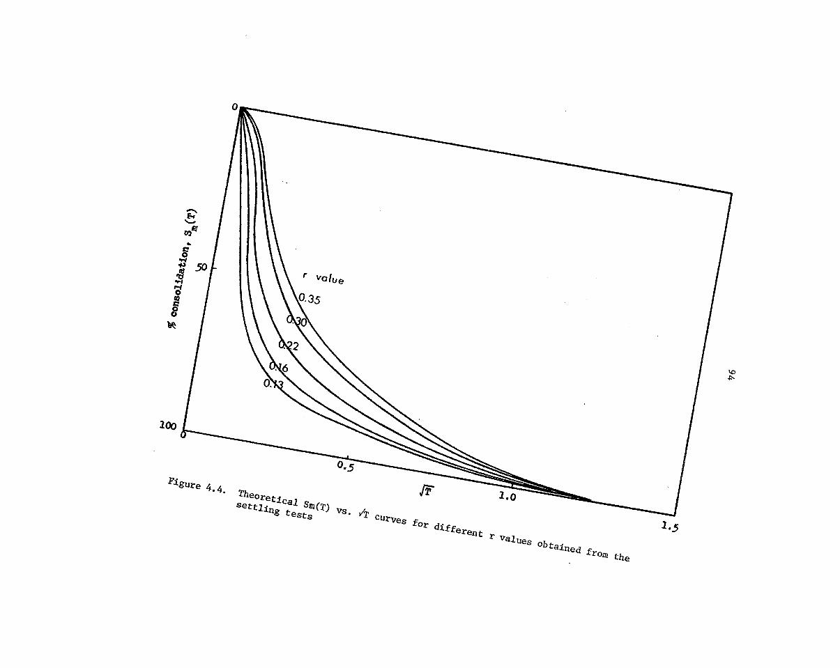
0
CO
s 30,
•ë
I ^o/ot
100
VO -fS
Pi gure 4.4.
The, settl
oreti cai yr
Sm(T) 1.0
tesc:" vs. /r curves for
diff, Great r
i.5
values Ob ta ined
the

95
CHAPTER V. CONCLUSIONS AND RECOMMENDATIONS
Conclusions
The findings of this study are the following;
1. The classical theories used by mining or chemical engineers for describing the settling mechanism of particles in a fluid emphasized entirely on the "sedimentation" phenomenon in which the weight of particles is solely supported by hydrodynamic forces, and neglected that particles will eventually come into con
tact, develop effective stresses and consolidate under their own weight. Hence, the theories are not adequate
for studying the settling behavior of the slurry in a containment area.
2. The WES interpretation of the settling column test results separates zone settling behavior from consolidation processes. This study indicates that zone settling behavior of the slurry is the result of self weight consolidation. In addition, if the time rate settlement of dredge materials is predicted according to the one-dimensional consolidation theory, as in the WES approach, the settling rate in the early consolidation period will be overestimated.
3. The interface, separating the clear supernatant water from the particle laden water, will not form in the tests with low initial concentration unless the average concentration of the slurry has reached certain value, i.e., critical concentration.
4. The self weight consolidation theory, developed by Lee and Sills (1981) and modified by Been and Sills (1981), is used to describe the zone settling behavior in this study. This study shows that the ratio, r, of actual to modified material height relates the theoretical consolidation curves to corresponding zone settling curves.
5. Based on the modified self weight consolidation theory, an approach for estimating the apparent coefficient of consolidation Cp, utilizing primarily the results of the settling column test, is feasible. The method should not only facilitate the test procedures for estimating

96
the Cp, but also yield a better prediction of the Cp because the method precisely defines the point at which self weight consolidation begins.
Recommendations for Future Study
Successful application of the large strain consolidation theory,
i.e.. Equation 1.17, depends very much on the reasonable assumptions
of the permeability, K, vs. the void ratio, e, and the effective
stress, a', vs. e relationships. Though the linear R vs. e and o'
vs. e relationships assumed by Lee and Sills (1981) facilitate the
solving of the highly nonlinear differential equation (Equation 1.17),
both assumptions can not be justified by the experimental results.
Further study on these two relationships is needed. The following
assumptions might make the model a better approximation of reality.
1. According to Equation 1.41, the permeability of soil seems to vary linearly with e3/l + e instead of 1 + e as assumed by Lee and Sills.
2. Been and Sills (1981) found that when the effective stress a' is very low, the a' vs. e relationship is not unique. Because the behavior of e in low effective stress range associates with the phenomenon of creep or viscous flow, a thermodynamic model might be needed for the study of the a' vs. e relationship.
97
REFERENCES
Been, K. and G. C. Sills. 1981. Self-Weight Consolidation of Soft Soils: An Experimental and Theoretical Study. Geotechnique 31, No. 4: 519-535.
Coe, H. S. and G. H. Clevenger. 1916. Methods for Determining the Capacities of Slime-Settling Tanks. American Institute of Mining Engineers Transactions 55, No. 9: 356-384.
Fitch, B. 1962. Sedimentation Process Fundamentals. American Institute of Mining Engineers Transactions 223: 129-137.
Gallagher, B. J. and Company. 1978. Investigation of Containment Area Design to Maximize Hydraulic Efficiency. U.S. Army Engineer Waterways Experiment Station, CE, Vlcksburg, Miss., Technical Report D-78-12.
Gaudin, A. M. and M. C. Fuerstenau. 1958. The Transviewer - X Rays to Measure Suspended Solids Concentration. Engineering and Mining Journal 159, No. 9: 110-112.
Gaudin, A. M., M. C. Fuerstenau and S. R. Mitchell. 1959. Effect of Pulp Depth and Initial Pulp Density in Batch Thickening. American Institute of Mining Engineers Transactions 214: 613-616.
Gaudin, A. M. and M. C. Fuerstenau. 1962. Experimental and Mathematical
Model of Thickening. American Institute of Mining Engineers Transactions 223: 122-129.
Gibson, R. E., G. L. England and M. J. L. Hussey. 1967. The Theory of One-Dimensional Consolidation of Saturated Clays. Geotechnique 17, No. 3: 261-273.
Hayden, M. L. 1978. Prediction of Volumetric Requirements for Dredged Material Containment Areas. U.S. Army Engineer Waterways Experiment Station, CE, Vlcksburg, Miss., Technical Report D-78-41.
Huston, J. 1970. Hydraulic Dredging. Cambridge, MD, Cornell Maritime Press, Inc.
Kynch, C. J. 1952. A theory of Sedimentation. Faraday Society Transactions 48: 166-176.
Laçasse, S. E., T. W. Lambe and W. A. Marr. 1977. Sizing of Containment Areas for Dredged Material. U.S. Army Engineer Waterways Experiment Station, CE, Vlcksburg, Miss., Technical Report D-77-21.

98
Lee, K. and G. C. Sills. 1981. The Consolidation of a Soil Stratum, Including Self-Weight Effects and Large Strains. International Journal for Numerical and Analytical Methods in Geomechanics 5: 405-428.
Lin, T. W., 0. G. Lara, R. A. Lohnes, and M. D. Dougal. 1981. Study of Sedimentation in Lake Panorama. Progress Report submitted to Central Iowa Energy Cooperative, Cedar Rapids, Iowa.
Mclaughlin, R. T. 1959. The Settling Properties of Suspensions. American Society of Civil Engineers Proceedings 85, No. HY12; 9-41.
Michaels, A. S. and J. C. Bolger. 1962. Settling Rates and Sediment Volumes of Flocculated Kaolin Suspensions. Industrial and Engineering Chemistry Fundamentals 1; 24t33.
Montgomery, R. L. 1978. Methodology for Design of Fine-Grained Dredged
Material Containment Areas for Solids Retention. U.S. Army Engineer Waterways Experiment Station, CE, Vicksburg, Miss., Technical Report D-78-56.
Palermo, M. R., R. L. Montgomery, and M. E. Poindexter. 1978. Guidelines for Designing, Operating, and Managing Dredged Material Containment Areas. U.S. Army Engineer Waterways Experiment Station, CE, Vicksburg, Miss., Technical Report DS-78-10.
Schaefer, V. R. 1980. Preliminary Investigation of Sedimentation in Lake Panorama, Iowa. Unpublished M.S. Thesis. Iowa State University Library, Ames.
Talmage, W. P. and E. B. Fitch. 1955. Determining Thickener Unit Areas. Industrial and Engineering Chemistry 47, No. 1: 38-41.
Taylor, D. W. 1948. Fundamentals of Soil Mechanics. New York, N.Y., John Wiley & Sons.
Terzaghi, K. 1925. Erdbaumechanik. Vienna, Franz Deuticke.
Terzaghi, K. and 0. K. Frohlich. 1936. Theorie der Setzung von Tonschichten. Vienna, Franz Deuticke.

99
ACKNOWLEDGMENTS
I wish to express my sincerest appreciation to Dr. Robert A. Lohnes
for all the assistance and guidance he provided during my study at Iowa
State University. His encouragement and discussions have made invaluable
contributions to this dissertation.
My appreciation also goes to Drs. Richard L. Handy, Turgut Demirel,
Ronald L. Rossmiller and Roger W. Bachmann for serving on my committee.
I thank my wife, Su-Men, who typed the original manuscript and en
dured many hardships during the thesis preparation period.
I gratefully acknowledge Central Iowa Energy Cooperative for funding
this research project and the support of the Engineering Research In
stitute of Iowa State University.

100
APPENDIX. TEST RESULTS
Results of Zone Settling Tests
The slurry height at various times was observed during the settling
column test without sample extraction. In Figures A-1 to A-5, the ob
served slurry height, H, is plotted versus /t, and the slurry height
corresponding to 100 percent self weight consolidation, for each
test is estimated. In addition, the t^g for each test results by apply
ing the /t-fitting method.

10 20 30 40 50
âïn'.
Figure A-1. The H vs. /t plot for test N-1
Test N-1, Cj= 75.3 g/l
Slope ratio R®2.91
tgQ= (31.5-9.2)^= 497 min.
Hioo* 10.

70'
60 \ G
Test N-2, 101.0 g/l
Slope ratio R = 3.^2
V (5^^-8-7)^=2052 min.
50 -
5
-p
S 40 jS
w 30
20
«100=13.3" «-
jTiaa, mini
Figure A-2. The H vs. /t plot for test N-2

10 20 30 40 50
JriMè, ate.
Figure A-3. The H vs. /t plot for test N-3
Ttet H-3, Cj= 147.0 g/l
Slope ratio R = 3.94
t^= (91.5-3.2)^- 7797 min.

Test N-4, 0^=191.5 g/l
Slope ratio R= 3.37
t_n= (88f= 7744 min. 60
50-
40-
30
«100= "—
20
10 20
Figure A-4. The H vs. /t plot for test N-4

Test N-5, c = 226,5 g/l
Slope ratio R= 2.8?
(75.7f= 5730 ain.
20
0 10 40 20 30 60 50 80 70 90
/Else, nin.
Figure A-5. The H vs. /t plot for test N-5

106
Results of Flocculent Settling Tests
Slurry samples were regularly withdrawn from the column for con
centration determinations in flocculent settling tests. Figures A-6 to
A-11 show the concentration profiles at various times for the settling
tests with different initial concentrations. The slurry height, H, was
also observed regularly in these tests, except for the two tests with
very low initial concentration L-1 and L-2, and H is plotted versus /1
in Figures A-12 to A-15.

' 0 rain Tfest W-1, c.= 76 g/l
10 min
•H 0) as 180 rain.
20 480 rain
0 100 200 300 Concentration, g/l
Figure A-6. The concentration profiles resulting from test W-1

70
min. 30 min. Test W-2, 99.1 g/l 60
90 min.
40
30 160 min.
600 min. 20
10
0
0 100 200 Concentration, g/l
300
Figure A-7. The concentration profiles resulting from test W-2

70 30 min.
(ô min.
Test W-3, 125.0 g/l 60 _90 min.
50 210 min.
40
30 720 min.
20
10
0 0 100 200 300
Concentration, g/l
Figure A-8. The concentration profiles resulting from test W-3

30'min. f!3 min.
Test W-4, c.= 190 g/l .90 min.
240 min.
20
10
0 100 200 300
Concentration, g/l
Figure A-9- The concentration profiles resulting from test W-4

s
70
60
50
40
I X 30
20
10
Test L-1, c.= 20 g/l 0 rain
15 mm
.
30 mir
I 60 mln.
100
Concentration, g/l
Figure A-10. The concentration profiles resulting from test 1—1

70 r
60 1 Test L-2, c.= 30 g/l 0 min. ^
50
1
40 1
1
30
\ \l 30 min.
20 j
10
60 min.
0 1
0 50 100 150
Concentration, g/l
Figure A-11. The concentration profiles resulting from test L-2

Test W-1, c.= 76 g/l
•g,
jTime, rain.
Figure A-12. The H vs. /t plot for test W—1

10 I I I
0 10 20 30 40 50 60 70 80 90
jTime, min.
Figure A-13. The H vs. /t plot for test W-2

70 L
60 \
a> -C 40
5 CO
30
20
10 0 10 20 30 40
jTime
Figure A-14. The H vs. yt plot for test W-3
Test W-3, 125 g/l
M M
_J . •
50 60 70 80 90 rain.

Test W-4, c.= 190 g/l
•S
rH CO
20
10 40 60 0 10 20 80 30 50 90 70
/Time, min.
Figure A-15. The H vs. /t plot for test W—4