Embed Size (px)
Citation preview
Securities Transaction Taxes: Macroeconomic Implications in a General-Equilibrium Model
Julia Lendvai, Rafal Raciborski and Lukas Vogel
Economic Papers 450 | March 2012
EUROPEAN
Economic and Financial Affairs
ECONOMY

Economic Papers are written by the Staff of the Directorate-General for Economic and Financial Affairs, or by experts working in association with them. The Papers are intended to increase awareness of the technical work being done by staff and to seek comments and suggestions for further analysis. The views expressed are the author’s alone and do not necessarily correspond to those of the European Commission. Comments and enquiries should be addressed to: European Commission Directorate-General for Economic and Financial Affairs Publications B-1049 Brussels Belgium E-mail: [email protected] This paper exists in English only and can be downloaded from the website ec.europa.eu/economy_finance/publications A great deal of additional information is available on the Internet. It can be accessed through the Europa server (ec.europa.eu) ISBN 978-92-79-22971-8 doi: 10.2765/25785 © European Union, 2012

Securities Transaction Taxes:Macroeconomic Implications in aGeneral-Equilibrium Model�
Julia Lendvaiy Rafal Raciborskiz Lukas Vogelx
Abstract
This paper studies the impact of a securities transaction tax (STT)on �nancial trading, stock prices and real economic variables in a closed-economy dynamic stochastic general-equilibrium model featuring �nancialfrictions. The model incorporates channels by which �noise trading�a¤ectsreal economic volatility. Firms�investment expenditure is related to thevalue of their outstanding shares. The model is calibrated to stylisedfacts of �nancial trading and �rms��nancing. The simulations suggestdistortive e¤ects of the STT on real variables similar to those of corporateincome taxation. At the same time, the STT reduces economic volatility,but this stabilisation gain is quantitatively modest.
JEL classi�cation: E22, E44, E62
Keywords: capital costs, �nancial markets, noise trading, securities trans-action tax
1 Introduction
The banking and �nancial crisis of recent years has been followed by calls (yet,less action) to reform the �nancial regulation in order to prevent the replayof events and improve the resilience of the �nancial sector. Given the massivecosts that bank rescues have in�icted on taxpayers, the demand to make the�nancial sector contribute to the �nancing of crisis-intervention costs has alsogained political voice and support (IMF, 2010). The political debate suggests�nancial sector taxation as a toolbox to mitigate structural problems and re-cover (some of) the budgetary costs of the bank rescue. In contrast to the
�The views expressed in this paper are views of the authors and do not necessarily corre-spond to positions of the Directorate-General for Economic and Financial A¤airs or the Eu-ropean Commission. We thank Thomas Hemmelgarn, Gaetan Nicodeme and Werner Roegerfor valuable comments and suggestions.
yEuropean Commission, DG Economic and Financial A¤airs; [email protected] Commission, DG Economic and Financial A¤airs; [email protected] Commission, DG Economic and Financial A¤airs; [email protected]
1

public discussion, however, there is little public �nance literature on �nancialsector taxation, its regulatory merits and drawbacks, and its potential to gener-ate government revenue. Furthermore, the existing empirical work looks fairlyinconclusive. Consequently, the governments that have taken action have beenlargely unguided by academic research (Keen, 2011).Against this background, we aim at contributing to this literature and pro-
vide an analysis of the securities transaction tax (STT) in a dynamic stochasticgeneral-equilibrium (DSGE) model. The main questions our model speci�ca-tion addresses are: (1) What is the STT�s long-term impact on �nancing costs,investment and economic activity? (2) Does the STT succeed in reducing (non-fundamental) volatility of asset prices and real economic variables?The model we use to address these questions is an RBC model featuring two
types of �nancial frictions. First, we incorporate short-term �nancial trade andallow for the presence of not fully rational traders, so-called �noise traders�whosetrading behaviour is a source of economic �uctuations in the model. Second, weintroduce a �nancing constraint which links �rms�investment spending to theiroutstanding share value. The structure of the model allows imposing a tax onsecurities transactions (STT). We calibrate our model to match some stylisedfacts about �nancial markets and �rms��nancing.While the adverse impact on the �nancing costs for companies�real invest-
ment is generally seen as the major potential drawback of an STT, the reductionof non-fundamental volatility is usually regarded to be its principal regulatorymerit. The model-based analysis in this paper makes an attempt to quantifyboth e¤ects and their macroeconomic implications. The exercise also discussesthe parameters that shape their relative importance.The contribution and novelty of discussing the STT in a DSGE framework
is the emphasis on the STT�s macroeconomic impact and the exposition ofrelevant transmission channels. The approach contrasts with partial equilibriumapproaches (e.g. Kupiec, 1996; Song and Zhang, 2005) that exclude feedbacke¤ects accross di¤erent markets and over time and conjecture the imapct ofSTTs on the real economy o¤-model.The main results are that a transaction tax generating tax revenue of 0.1% of
GDP would (1) increases capital costs by 4-5 basis points, implying a long-term0.4% decline in the capital stock and a 0.2% decline in real GDP, and (2) reducethe volatility of physical investment and output by 4% and 1% respectively.Section 2 of the paper reviews STT debate, listing the main arguments for
and against STTs to place our analysis in context. Section 3 develops a DSGEmodel with noise trading and STT as the paper�s analytical framework. Section4 presents the parameterisation of the model. Section 5 presents the scenariosand simulation results and compares them to related �ndings in the literature.Section 6 summarises and concludes.
2
2 The STT debate
The paper contributes to the still inconclusive debate on the merits and draw-backs of STTs. Matheson (2011) and Schulmeister et al. (2008) give a compre-hensive survey of the debate; Hemmelgarn and Nicodeme (2010) and Schwertand Seguin (1993) provide a concise list of pros and cons. This section providesa brief review of the key arguments to locate the contribution of our analysis.
2.1 Asset price volatility
Advocates of the STT have traditionally focused on the instrument�s abilityto curb short-term speculative trading in �nancial markets by raising the costof �nancial transactions. The idea is that speculative trading rests on non-fundamental information ("noise"). Curbing short-term trade could in this viewreduce asset mispricing and market volatility by reducing noise trading as wellas the related waste of resources (from the society�s perspective) in the �nancialsector (e.g., Stiglitz, 1989; Summers and Summers, 1989).The volatility-reduction argument rests on the assumption that an STT cor-
rects ine¢ ciencies instead of adding an additional distortion, or, at least, thatthe corrective e¤ect dominates distorting ones. Market volatility decreases ifthe tax succeeds in curbing non-fundamental trades. But critics argue thatthe trade-reducing impact of STTs could back�re. The tax may eventually in-crease asset price volatility in the market, because the trade volume reductionincreases the impact of individual transactions on asset prices and price volatil-ity (e.g., Habermeier and Kirilenko, 2003). In general, individual transactionscause larger price �uctuation in thinner markets.Additionally, STTs cannot discriminate between fundamental-based and non-
fundamental trades and may therefore weaken �nancial market adjustment andresilience. Restricting short-term trades by increasing the trading costs may re-sult in a build-up of larger imbalances and increasing costs of risk hedging. Sinceall transactions are taxed at equal rates and independent of their risk pro�le,the STT may not reduce risk-taking and fragility in the �nancial sector (Keen,2011). The tax should target trading risk rather than the trading frequency inorder to make a contribution to �nancial market stability.Moreover, there are many practical problems with introducing a general
STT in the open economy. New �nancial instruments may be designed to avoidtaxation and would further increase the opacity of the �nancial sector. Interna-tionally integrated markets add the dimension of tax avoidance by cross-bordertransactions. To cope with the practical problems, the tax would have to be im-posed on the broadest possible base and internationally coordinated. What con-situtes the "broadest possible base" is likely to change with STT introduction,requiring dynamic adjustment. The success of an encompassing implementationis far from certain.Limiting the STT to spot transactions that are easier to track, such as
standard account transactions, or stock and bond purchases and sales, insteadof including derivative trading is likely to limit the problem of tax avoidance,
3
but skews the tax burden towards households and �rms that have little to dowith high-frequency trading and the associated volatility of asset prices.STTs are already more than a hypothetical tool. Variants of STTs have been
implemented in several countries (see IMF, 2010; Matheson, 2011; Schulmeisteret al., 2008; Summers and Summers, 1989), and attempts have been made toquantify their impact on market volatility. While the empirical evidence isscarce, see Matheson (2011) and Schulmeister et al. (2008) for comprehensivesurveys, it provides no robust support for a market-stabilising e¤ect of the STT.Hau (2006), e.g., �nds that increasing transaction costs has increased the stockprice volatility in the French stock market. More precisely, he �nds that 20%higher transaction costs have led to 30% increase in the hourly volatility ofindividual stock prices. Hau concludes that higher transactions costs and STTsin particular should be regarded as volatility increasing. For the United States,Jones and Seguin (1997) report a positive e¤ect of transaction cost reduction ontrade volumes for NYSE listed shares, which has reduced the volatility of shareprices. Baltagi et al. (2006) study the Chinese case and �nd that the stamp taxhas reduced trade volumes and increased market volatility. According to theirresults, an increase in the tax rate from 0.3 to 0.5% has increased transactioncosts by one third and reduced trading volumes by one third. The results inBaltagi et al. (2006) also suggest negative e¤ects of the STT on stock markete¢ ciency, as markets take more time to absorb external shocks. Hence, theshort-term trading that the STT is meant to eliminate is not empirically provento be detrimental to price recovery.Partial-equilibrium models of �nancial markets with heterogenous agents
and complex market structure obtain mixed results. While Westerho¤ and Dieci(2006) �nd an STT imposition on all transactions to reduce price volatility ac-cross markets, Mannaro et al. (2008) conclude that the STT increases assetprice volatility by reducing trading values. Demay (2006) �nds that the STTfavours long-term investment over short-term speculation, but also punishesfundamental-based trading rules compared to trend extrapolation in exchangerate markets. Demay (2010) concludes that STTs increase asset mispricingbeyond certain thresholds by reducing short-term trading in reaction to fun-damantal changes. Pellizzari and Westerho¤ (2009) stress the sensitivity ofresults with respect to the micro structure of �nancial markets. They contrastsituations in which the STT increases price volatility by lower trading volumeswith cases in which an STT e¤ectively crowds out speculative trades. The ex-perimental study by Hanke et al. (2010) �nds the e¤ects of a Tobin tax onexchange rates to depend on the existence of tax havens and on market size.The STT reduces short-term speculation, but market e¢ ciency in taxed mar-kets decreases when tax havens exist. A complementary paper by Kirchler etal. (2011) concludes that an encompasing Tobin tax in exchange rate marketshas no impact on exchange rate volatility. Xu (2010) �nds the e¤ect of a Tobintax on the exchange rate volatility introduced by noise traders to depend onthe market structure (exogenous versus endogenous entry) and the interactionbetween the tax and other trading costs.Finally, the banking and �nancial crisis of 2008 does not provide strong
4
arguments for favouring a STT to tax the �nancial sector. Although the STTmay reduced short-term trading and asset price volatility, a clear connectionbetween short-term trading and long-run cycles of asset mispricing (bubbles)has not yet been established. Instead, the instruments that caused the distressand failure of �nancial institutions in the 2008 crisis did not belong to theset of frequently traded assets. The STT does not address leverage, maturitymismatch, currency mismatch and the underestimation of investment risk (e.g.,Hemmelgarn and Nicodeme, 2011; Matheson, 2011).
2.2 Capital costs
The strongest objection against the STT is that it may harm rather than helpreal economic activity by reducing equity prices and increasing the capital costsfor real investors. In an economy producing with decreasing marginal returns tophysical capital, higher capital costs reduce the long-term capital stock, labourproductivity and real output. The strength of the capital-cost e¤ect woulddepend on the tax rate and the investment horizon of savers. A low tax rateand long-term focus should limit the impact on fundamental investment.1
The STT may a¤ect capital costs and investment even if applied exclusivelyto the secondary market. Lower liquidity in the secondary market may increasethe interest premium that investors charge to insure against the cost of pre-mature disinvestment linked to a materialisation of investment risks or to anunforeseen tightening of the individual budget constraint. Similarly, �nancialconstraints on real investment tighten if the STT reduces equity prices and thevalue of �rms.Broad-based STT application to all �nancial transactions could also a¤ect
the market structure in the real economy. IMF (2010) and Shackelford et al.(2010) argue that a broad STT imposition on business-to-business transactionssupports economic concentration on goods and factor markets. Taxing business-to-business transactions instead of �nal values implies a cascading tax burdenon the production by non-integrated �rms, which provides incentives for thevertical integration of production lines.The existing empirical evidence supports the view that a STT imposition
reduces equity prices. Analysing the impact of the UK stamp duty, Bond etal. (2004) establish a positive impact of (announced) tax cuts on the relativeprice of more frequently traded shares. The empirical research does not addressthe e¤ect on �nancing costs. Theoretically, lower stock values are likely to raisethe �rms�capital costs for equity and debt �nance: The negative STT impacton stock prices reduces the capital raised by equity issuance at given tradingfrequencies. A falling �rm value also reduces debt �nance by tightening �nancialconstraints and/or increasing the risk premium that lenders ask to compensatefor the fall in the collateral value.
1From a general-equilibrium perspective, STT introduction may additionally allow reducingother taxes on capital and complementary factors that increase the costs of capital (e.g.,Summers and Summers, 1989).
5

2.3 Tax revenue
Besides the idea that the tax could substantially dampen excessive trading, thesecond principal argument in favour of the STT is its potential to generate sub-stantial tax revenue, which would help governments to cope with the budgetarycosts and repercussions of the �nancial and economic crisis. To ensure substan-tial revenue and limit tax avoidance, the revenue-oriented imposition of STTsshould favour broad tax bases, so that substantial revenue can be collected atlow rates. As illustrated in the previous section for the example of cascadinge¤ects on non-integrated �rms, broadening the tax base does not necessarily re-duce the implied economic distortions. Granting exceptions, on the other hand,would give rise to strategies of tax avoidance (e.g., IMF, 2010).More fundamentally, the STT illustrates once more the trade-o¤between the
corrective e¤ects of taxations and the collectable tax revenue, a trade-o¤ thatderives from the endogeneity of the tax base. To the extent the tax succeedsin dampening excessive trading the base, the collected STT revenue declines.At the end, the tax may be levied predominantly on fundamental-driven trans-actions. The tax revenue is highest, on the other hand, if the tax has littledampening impact on speculative trading.2
An additional concern relates to the STT�s overall impact on the governemntbudget balance and government debt. How should government bonds and re-lated derivatives be treated? Existing proposals exempt government debt fromthe STT to avoid an increase in �nancing costs for the government, which coulddecrease or even o¤set the positive impact of additional tax revenues. Theexclusion of public debt would give an advantage to the government and dis-tort �nancial investment towards the public sector. Depending on the size ofthe premium one may wonder whether cheaper debt could invite overborrowingand �scal pro�igacy. Exempting public debt derivatives like default insurancefrom the STT would, on the other hand, exclude a category of assets that someobservers think has aggravated the euro area�s problems ("speculation againstgovernments").The subsequent sections of the paper relate to all three aspects, without ad-
dressing the entire set of problems, objections and caveats. The modelling andthe simulations focus on: (1) the STT�s impact on capital costs and real eco-nomic activity; and (2) the STT�s impact on non-fundamental ("speculative")trading and associated asset price volatility. Focusing on the taxation of corpo-rate equity transactions, the model excludes �nancial derivatives. Furthermore,we do not address technical problems (e.g., transparency of transactions, tax col-lection) and questions of tax avoidance or evasion in internationally integrated�nancial markets.
2Summers and Summers (1989) argue in this line that an STT with little impact on �nancialmarkets would raise tax revenue and �scal space and allow reducing more distortionary taxes.In this scenario the STT would be a more e¢ cient revenue source than alternative taxes. Ifa substantial part of the tax incidence fell on asset holders (instead of real wages), the STTwould also be highly progressive.
6

3 Model description
To study the impact of STTs on the economy, the paper incorporates �nan-cial frictions in an otherwise standard closed-economy RBC model. Financialfrictions are introduced along two dimensions:Firstly, we introduce a sector of �nancial traders engaged in short-term trad-
ing of securities. Financial traders borrow from households, invest in stocks,receive returns on the investment, pay back the outstanding loans and consumethe rest. A fraction of the traders are "noise traders" in the sense of De Long etal. (1990) and Shleifer and Summers (1990). Noise traders have noisy expecta-tions about stock returns that may deviate from rational expectations based oneconomic fundamentals. Non-fundamental "noise shocks" that capture changesin the noise traders�beliefs increase the volatility of asset prices and trading.Secondly, �rms� borrowing for investment in physical capital is restricted
by what we call a �nancial constraint. In particular, we assume that a �rm�sinvestment in physical capital cannot exceed a given fraction of the �rm�s stockvalue. Such a constraint would, e.g., occur if banks treat the stock value asindicator for a �rm�s economic conditions, so that the amount of loans they arewilling to provide for real investment depends on the stock market valuation ofthe �rm. If new investment by the �rm is (partly) credit-�nanced, the invest-ment will be limited by the valuation of �rm�s stocks. Another link might bethe information value of stock prices for decisions by the �rm�s management. Inour paper we do not model the bank sector explicitly. The �nancing constraintis a shortcut to capture the link between the stock value and the �nancing of�rms. This link link between �rm value and investment has been establishedempirically (see, e.g., Baker et al., 2003; Barro, 1990; Bond et al., 2011; Chenet al., 2007; Fazzari et al., 1988; Morck et al., 1990).The model assumes that households have a long-term investment horizon
and own a �xed share of total equity. The equity owned by households is notpublicly traded and accounts for a larger part of total equity. This is meant tore�ect the European model of corporate �nance, where a relatively limited partof investment is funded by the public issuance of stocks. Noise and fundamentaltraders, in contrast, have short (2-period) planning horizons, which emphasisesthe short-term return orientation of their transactions. The traders borrow inthe credit market from non-trader households at risk-free rates and invest inpublicly-traded stocks. In the following period, they earn the returns on theirrisky investment and pay back their debt including the (risk-free) interest.Short-term trading generates transaction costs by using limited resources
such as time and e¤ort. Imposing "wasted" transaction costs captures aggregateine¢ ciencies or the ressource use of short-term trading. The model introducesa tax (STT) on the short-term transactions to analyze its potentially correctiverole.The model determines the stock value of �rms as the expected discounted
�ow of future dividends. The value increases with positive noise shock anddeclines in response to transaction costs and the STT. Falling stock prices in-crease the costs and/or reduce the ability for �rms to raise capital through
7
equity issuance, debt issuance or bank credit. The before-tax return on invest-ment that �nancial investors require increases. With falling marginal returns tocapital, the introduction of an STT translates into equilibria with lower capitalstock and lower labour productivity.Contrary to previous analyses, this paper integrates noise trading and the
STT in a general-equilibrium model that links �nancial and real sector vari-ables. Previous theoretical models to analyse �nancial sector taxation haveadopted a partial equilibrium view of �nancial markets (e.g., Kupiec, 1996;Song and Zhang, 2005) and conjectured the impact on the real economy outsidethe model. Focusing on general equilibrium e¤ects and the interaction between�nancial and real sectors, the structure of �nancial markets and trading is keptsimple in our model. We distinguish two types of traders, but assume an atom-istic market structure. Although the consequences of one group�s behavioura¤ect the other type of traders, the atomistic market structure excludes strate-gic interaction. Consequently, our focus is di¤erent from heterogeneous-agent,partial-equilibrium models of the �nancial market (e.g., Demary, 2006; Demary,2010; Mannaro et al., 2008; Hanke et al., 2010; Kirchler et al., 2011; Pellizzariand Westerho¤, 2009; Westerho¤ and Dieci, 2005) in which the impact of STTimposition on asset prices and transaction volatilities is found to depend on themarket structure.As further simpli�cation, we use a closed-economy framework and assume
the STT to be e¤ectively implementable and enforceable. The analysis abstractsfrom the challenge of tax evasion in internationally integrated �nancial markets.Alternatively, the setup can be interpreted as representing the world economyunder globally uni�ed transaction taxation.The model focuses on corporate equity and excludes other classes of risky
assets. In particular, the model excludes derivatives, which are not easily in-corporated in a general-equilibrium framework, despite the fact that derivativesaccount for a large share of transactions in real-world �nancial markets today.To align sequences of �nancial and real investment decisions, and despite the
quantitative importance of high-frequency asset trading, we impose homogenoustime intervals for �nancial trading and decisions on real economic variables. Inline with standard practice in business-cycle models, the time interval corre-sponds to quarters of years. The following subsections describe the details ofthe model structure.
3.1 Households
The household sector consists of two types of households. A fraction sl are thestandard in�nitely-lived households. These households consume, work and owna �xed fraction of �rms�equity on which they earn dividends. The variablesrelating to the in�nitely-lived households are indexed by the superscript l. Theremaining fraction 1 � sl are short-horizon �nancial traders. These tradersborrow from the in�nitely-lived households at the risk-free interest rate andinvest the funds they have borrowed into stocks. Traders borrow and invest inperiod t. In the subsequent period t + 1, they receive dividends on their asset
8
holdings and sell the assets. The traders use the proceeds from dividends andthe selling of assets to settle their debt with the in�nitely-lived households andthen consume the remaining income. The variables relating to the traders areindexed by the superscript T . All variables in the model are de�ned in percapita terms.The group of traders consists of two di¤erent sub-groups. The fraction sn
of trader households are so-called �noise traders�, indexed by the superscriptN . Noise traders have noisy expectations about the future share return in thesense that their expectations may deviate from rational expectations by a noiseshock. The share 1� sn of traders forms rational expectations about the stockreturn given the model structure and the occurence of shocks. These tradersare labelled as informed traders by the superscipt I.
3.1.1 In�nitely-lived households
The in�nitely-lived households l maximise welfare:
maxClt;Lt;B
lt
E0
1Xt=0
�t�lnClt �
!
1 + �L1+�t
�(1)
subject to the budget constraint:
Clt+Blt+P
shllt alt =
�1� � l
�WtLt+Rt�1B
lt�1+
�P shllt +DIVt
�alt�1�T lst (2)
where Clt is consumption, Blt are holdings of risk-free assets and a
lt holdings
of corporate equity. The equity held by the in�nitely-lived households is notpublicly-traded and constitutes a �xed proportion � of total equity (traded andnon-traded) in the economy. The value of assets that are never traded, alt, isuna¤ected by the STT. They may be considered to proxy not only for privateequity but also for investement �nanced by credit, which is also not subjectto the STT. The value of a unit of the non-traded assets is P shllt . They bringdividend DIVt per asset unit that is paid in period t. Rt�1 is the gross interestrate on the risk-free asset �xed in t � 1 and paid in t, Lt is per-capita hoursworked, Wt is the nominal wage, � l is the labour income tax rate, and T lst arelump-sum taxes.The in�nitely-lived households��rst order condition (FOC) for optimal con-
sumption, labour supply and �nancial investment are:
!L�t Clt =
�1� � l
�Wt (3)
�lt = 1=Clt (4)
�lt = �RtEt�lt+1 (5)
1 = �Et
"�lt+1
�lt
�P shllt+1 +DIVt+1
P shllt
�#(6)
9

Equation (6) is the FOC with respect to the stock holding of the in�nitely-livedhouseholds. It is the usual Euler equation, which stipulates that the householdin equilibrium should be indi¤erent between consuming one additional unit ofconsumption today and investing this consumption unit into equity at priceP shllt per unit of equity, selling this unit of equity next period at price P shllt+1 ,and consuming the proceeds plus the dividendDIVt+1 that additionally accrues.Since the amount of the households equity holdings alt does not enter the Eulerequation, it can be regarded as determining the value P shllt of the non-tradedequity.
3.1.2 Short-lived traders
Each trader household exists for two periods only. The traders borrow fromin�nitely-lived households and invest the funds into publicly-traded corporatestocks. The pro�t from this �nancial investment is consumed. The amount ofborrowing and investment derives from the maximisation of traders�utility:
maxCT;jt ;aT;jt
�Ejt logCT;jt+1 (7)
subject to the traders�budget constraint:
EjtCT;jt+1 = �w + Ejt
�P sht+1 +DIVt+1
�aT;jt �RtP sht a
T;jt (8)
�c+ �STT
2P sht
�aT;jt
�2where j = I;N denotes the groups of informed traders and noise traders, respec-tively. In analogy to the non-trader households, CT;jt+1 is traders�consumptionand aT;jt their asset holding. The variable P sht denotes the price of tradedstocks 1� �. In period t, traders borrow the amount of P sht a
T;jt from the non-
trader households and invest these funds in stocks. In period t+ 1, the tradersreceive the return on the investment
�P sht+1 +DIVt+1
�aT;jt net of transaction
cost (c), STT (�STT ) payments and a lump-sum tax T ls;Tt . The traders returnthe borrowed funds plus interest to the non-trader households (RtP sht a
T;jt ) and
consume the remaining pro�t plus the �x endowment �w.The endowment �w is added to the budget constraint (8) to exclude the
occurence of negative values for trader consumption and does not a¤ect anyother result.The conceptual di¤erence between transaction costs c and the STT is that
the transaction cost consumes resources whereas the transaction tax transfersresources to the government budget. The transaction costs enter the resourceconstraint of the economy. They can be understood as the resource cost oftrading in the sense of Summers and Summers (1989), i.e. the amount of labour,capital and skill absorbed by the �nancial system.The real ex-post stock return for traders that liquidate their positions in
period t+1 can be de�ned as Rsht+1 ��P sht+1 +DIVt+1
�=P sht . Informed traders
have rational, i.e. model-consistent, expectations about the future return, i.e.
10

EItRsht+1 = EtR
sht+1. The noise traders�expectations deviate from rational ex-
pectations by a random noise shock:
ENt Rsht+1 = EtR
sht+1 + �t (9)
with �t � N (��; ��). The traders� borrowing and investment decisions aredetermined by the FOCs:
Etc+ �STT
CT;It+1
aT;It = EtRsht+1 �RtCT;It+1
(10)
ENtc+ �STT
CT;Nt+1
aT;Nt = ENtRsht+1 �RtCT;Nt+1
(11)
Consumption by informed and noise traders in period t is given by:
CT;It = �w +�P sht +DIVt
�aT;It�1 �Rt�1P sht�1a
T;It�1 (12)
�c+ �STT
2P sht�1
�aT;It�1
�2
CT;Nt = �w +�P sht +DIVt
�aT;Nt�1 �Rt�1P sht�1a
T;Nt�1 (13)
�c+ �STT
2P sht�1
�aT;Nt�1
�2Traders� total per-capita consumption is the weighted sum of per-capita con-sumption levels of informed and noise traders:
CTt = (1� sn)CT;It + snC
T;Nt (14)
Analogously, the total stock portfolio of traders is:
aTt = (1� sn) aT;It + sna
T;Nt (15)
in per-capita terms.
3.2 Firms
Firms choose employment, the capital stock (Kt) and investment (It) to max-imise the discounted �ow of expected future dividends. The future dividendsare discounted by the stochastic discount factor of the in�nitely-lived house-holds who own the majority of the corporate equity. Formally, the optimisationproblem of �rms is:
maxLt;Kt;It
1Xt=0
��lt
�l0DIVt (16)
11
where �lt is the Lagrange multiplier of the budget constraint of in�nitely-livedhouseholds. Corporate dividends are the after-tax corporate income net of thewage bill, adjustment costs and investment expenditure:
DIVt � (1� � c) (Yt �WtslLt) + �c�Kt�1 � It (17)
where � c is the corporate tax rate, � is the depreciation rate of physical capital,and capital depreciation is tax-deductible.The maximisation of dividends is subject to three constraints, namely the
production technology:
Yt = At (Kt�1)1��
(slLt)� (18)
the law of motion for the capital stock:
Kt = (1� �)Kt�1 + It (19)
and a �nancing constraint for investment:
It 6 ��Et
"�lt+1
�lt
��P shllt+1 + (1� �)P sht+1
�#(20)
The �nancing constraint (20) states that the opportunity of raising funds fornew investment by long-term borrowing from non-trader households or stock is-suance is constrained by the current value of the �rm as re�ected in the equityvalue. The sensitivity of investment to the stock market performance is docu-mented empirically in the literature (e.g., Baker et al., 2003; Barro, 1990; Chenet al., 2007; Fazzari et al., 1988; Morck et al., 1990). The investment con-straint (20) is compatible with alternative hypotheses about the link betweenthe stock market value and investment. E.g., banks could use the �rm�s stockvalue as signal of the �rms economic health and make the volume and price ofloans depend on the �rm�s valuation. If new investment by the �rm is (partly)credit-�nanced, investment will be limited by the valuation of �rm�s stocks. The�nancing constraint is a mechanism/shortcut to capture the empirical link be-tween stock value and investment in a stylized manner. Alternative hypothesesfocus on the signaling value of equity prices for investment decisions (e.g., Bondet al., 2011, Chen et al., 2007, and Morck et al., 1990).The equity value of the �rm consists of two types of assets: value of publicly-
traded stocks (1� �)P sht and of private equity �P shllt . Parameter � governs theshare of the long-term private equity holding in total equity. While �rms mayhave a preference for �nancing by long-lived households, � indicates an upperbound for the funds that these investors are able to o¤er. One explanation forwhy �rms may have a prefererence for private equity is that this type of (owner)investors require lower returns, making �nancing cheaper. Yet, investors whoset up a �rm are likely to have limited �nancial resources and will need to turnto public o¤erings for additional capital. The value of � should be relativelylarge in Europe, however, as European �rms do not extensively rely on the
12

stock exchange to raise capital to invest and more frequently rely on directinvestment by owners (private equity) and loans.3
The maximisation of future dividends (17) under the constraints (18), (19)and (20) gives the FOCs for �rm�s labour demand, capital and investment :
�YtslLt
=Wt (21)
Qt = �Et�lt+1
�lt
�(1� � c) (1� �) Yt+1
Kt+ � c� + (1� �)Qt+1
�(22)
Qt = 1 + �t (23)
where �t and Qt are the Lagrange multipliers on the �nancing constraint andthe capital accumulation equation respectively in terms of consumption utility.
3.3 Government
The government consumes an exogenous amount of goods (Gt) and receivestax income from wages, corporate income and �nancial transactions. Currentgovernment debt (BGt ) is the sum of outstanding government debt, debt serviceand the primary de�cit:
BGt =Rt = BGt�1 +Gt � � lWtslLt � slT lst � � c (Yt �WtslLt) (24)
+� c�Kt�1 � (1� sl)�STT
2P sht�1
�(1� sn)
�aT;It�1
�2+ sn
�aT;Nt�1
�2�Lump-sum taxes T lst adjust endogenously to keep the government debt-to-GDPratio, BGt =Yt, constantly at its target level BY . The use of lump-sum taxesto stabilise the debt-to-GDP ratio eliminates the income e¤ect of the STT.Reducing distortive instead of lump-sum taxes to rebate the STT receipts wouldtend to improve the overall assessment of STT introduction in e¢ ciency terms.The setup in this paper, which isolates the STT�s distortionary e¤ects without,at the same time, lowering other distortive taxes to reimburse the STT revenue,implies a rather critical assessment of STT-related ine¢ ciencies.
3.4 Aggregation and equilibrium
With the total number of stocks normalised to one, the per-capita stock portfolioof non-trader households is:
alt = �=sl (25)
and the per-capita stock portfolio of traders is:
aTt = (1� �) = (1� sl) (26)
3 It could be argued that the value of �rms owned directly by households in form of privateequity is not fully observed by loan providers and can therefore not be used (fully) to assess the�rms�capacity of credit repayment. Publicly-owned equity should be given a higher weight inthe �nancing constraint in this case. However, we do not make such distinction in this paper.
13
The non-traders� risk-free assets, which consist of government bonds and thefunds lent to traders, equals:
Blt =1
sl
�BGtRt
+ (1� sl)P sht aTt�
(27)
Aggregate per-capita consumption is:
Ct = slClt + (1� sl)CTt (28)
Total employment in per-capita terms is slLt as the trader households do notwork.Factor, �nancial and goods markets clear in equilibrium. The market clear-
ing in the stock market implies:
at = slalt + (1� sl) aTt = 1 (29)
Market clearing in the market for risk-free assets implies:
Blt =BGt + (1� sl)P sht aTt
sl(30)
Aggregate demand is the sum of private consumption, investment, governmentpurchases and adjustment costs is aggregate demand. In equilibrium, aggregatedemand minus the endowment �w is equal to aggregate production Yt:
Yt = Ct+Gt+It++(1� sl)c
2P sht�1
�(1� sn)
�aT;It�1
�2+ sn
�aT;Nt�1
�2��(1� sl) �w
(31)which can also be understood as the ressource constraint of the closed economy.
4 Parametrisation
The parameters for the real and �nancial sectors and the exogenous processesneed to be quanti�ed prior to simulations. The parametrisation is summarisedin Table 1. Table 2 reports the steady-state ratios for key model variables asimplied by the parameter choices.
4.1 Real economy
The parametrisation of the real economy part is standard in the RBC literature.The discount factor is set to � = 0:99, which implies an annualised steady-staterisk-free interest rate of 4%. The long-lived households�weight of the disutilityof labour is set to ! = 5, which implies a steady-state employment of around0.19 of households�time endowment. The elasticity of labour supply is set to1=� = 1, which is standard in the DSGE literature, although upper-bound inmicroeconometric estimates of labour supply.
14
The labour share in the production function, which equals the steady-statewage share, is � = 0:64. The depreciation rate of physical equals � = 0:025,which implies an average depreciation period of 2.5 years. Both values arestandard in the literature. Together with the investment share of 23% of GDP,the depreciation rate implies a steady-state capital stock value of around 2.5times GDP. Steady-state total factor productivity A is normalised to 1.The steady-state shares and parameter values for the government sector
correspond to EU average values. Government purchases account for circa 20%of GDP. The labour income tax rate is 40% and the corporate income tax rate20%. The target level for public debt equals 50% of GDP.
4.2 Financial sector
Parameter choices for the �nancial sector are informed by data on trading vol-umes and the empirical literature on trading behaviour. In the benchmarkcalibration the share of stocks owned by non-trader households is set to � = 0:8to match observed ratios of quarterly stock market turnover over the total valueof outstanding corporate assets.The share of noise traders is set to sn = 0:5 in line with evidence on trading
behaviour in (foreign-exchange) markets (e.g., Cheung et al., 2004; Menkho¤,2001; Menkho¤ and Taylor, 2007; Oberlechner, 2001). Based on surveys amongmarket participants, these studies conclude that approximately 50% of trad-ing in these markets at the quarterly horizon is based on non-fundamental asopposed to fundamental information. In the sensitivity analysis, we also con-sider alternative values, namely � = 0:6 and � = 0:0 as well as sn = 0:25 andsn = 0:75.The benchmark calibration uses anSTT rate of 0.14%, which generates a
steady-state tax revenue of around 0.1% of GDP. The e¤ective tax rate of 0.14%is at the upper end of recent policy proposals (e.g., IMF 2010; Matheson, 2011;Schulmeister et al., 2008), although Summers and Summers (1989) suggest anSTT rate of up to 0.5%.
4.3 Exogenous shocks
The simulations consider the response of the economy to fundamental and non-fundamental disturbances, namely technology (TFP) and noise shocks, in thepresence of an STT. The focus on TFP shocks as real disturbances derives fromthe RBC literature�s �nding that TFP shocks are able to account for large partsof the observed volatility in real variables at business-cycle frequency. The TFPshocks is an AR(1) process with white-noise innovation "at :
lnAt = (1� �a) ln �A+ � lnAt�1 + "at (32)
In line with TFP estimates based on the Solow residual, the persistence of theTFP shock is �a = 0:95 and the standard deviation of the stochastic innovation�a = 0:0072. The noise shock is white noise "�t :
�t = "�t (33)
15

to capture eratic changes in noise traders�expectations and market sentiments.4
The standard deviation of the innovation �� = 0:0707 is choosen to generate inthe model a volatility of the return on stocks that is close to historic values of thestock return volatility in OECD countries (e.g., Kupiec, 1991). The stochasticinnovations "at and "
�t are assumed to be uncorrelated. TFP and noise shocks
are applied together throughout the simulations.
Name Symbol Value
Discount factor � 0.99Elasticity of labour supply ��1 1.00Labour weight in utility ! 5.00Labour share in production � 0.64Capital depreciation rate � 0.025Financing constraint � 0.025Public debt-to-GDP target BY 0.50Labour tax rate � l 0.40Capital tax rate � c 0.20STT rate �STT 0.0014Long-term share holding � 0.80Share of noise traders sn 0.50Trader endowment $ 0.10Tax rebate to traders sT 0.00Financial transaction costs c 0.01Persistence of TFP shock �a 0.95Steady-state TFP A 1.00Steady-state noise �� 0.00Standard deviation of TFP shock "a 0.0072Standard deviation of noise shock "� 0.0707
Table 1: Model parameters
5 Results
5.1 STT in the benchmark model
This subsection presents simulation results that gauge the impact of an STT inthe benchmark model with the parameterisation as described in the previoussection. The STT rate is set to 0.14% to raise a tax revenue of 0.1% of GDP inthe steady state.The STT�s impact on �nancial variables and economic aggregates is sum-
marised in Table 3. Values in the �rst column ("mean") report the percentage
4Non-zero persistence of the noise shock would imply a systematic component in the respnseof noise traders to disturbances that should better be integrated in the traders�decision rules.
16

Steady-state ratio Value
Y 1.00CY 0.68IY 0.23GY 0.10BG
Y 0.50KY 9.10L 0.36
Table 2: Steady-state ratios
change in the steady-state level in response to the introduction of the STT. Thesecond colum of results ("std/mean") shows the percentage change between thestandard deviation of the variables with and without STT.
Impact of STT on mean values and volatilitiesMean (%) Std (%)
Output 0.19 0.99Capital 0.43 0.15Investment 0.42 3.59Consumption 0.02 3.25Employment 0.06 8.28Real wage 0.14 0.34Share trade 8.40 12.25Share price 8.40 1.74
Mean (pp) Std (%)Return on shares 1.25 8.61Riskfree return 0.00 7.59Return on physical capital 0.04 1.57Transactions costs/GDP 0.06 2.61STT revenues/GDP 0.09
Note: The table compares scenarios without and with STT and reportsthe percentage (%) or percentage point (pp) changes in the mean andthe standard deviation of the variables for identical shocks.
Table 3: STT e¤ects in the benchmark model
The results in Table 3 illustrate two main e¤ects from introducing an STT.First, the introduction of the STT leads to a reduction in the price of thetraded equity and an increase in the pre-tax stock return in the long run (seethe �mean�column). The increase in the pre-tax return on capital required forinvestment increases the �nancing costs for �rms. As a result, investment andthe stock of productive capital decline by around 0.4%. Output, consumption
17

and employment decline as well in the long run in response to the decline in thecapital stock, lower labour productivity and falling income. Real GDP declinesby 0.2% in the long term, which is sizable for an STT rate of 0.14%.Second, the STT leads to a reduction in short-term trade and thereby damp-
ens non-fundamental �uctuations in real aggregates. According to the resultsin Table 3, introducing an STT of 0.14% would reduce the normalised volatilityof investment by circa 4% and the one of output by circa 1%.The STT-related decline in the volatility of �nancial and real variables also
applies to the response to TFP shocks only. The share value �uctuations inresponse to TFP shocks re�ect changing expectations about the pro�tabilityof investment. Introducing an STT in this context dampens the adjustmentof the capital stock, which also translates into lower volatility of investment,consumption and output. This volatility reduction is not unambigously positivefrom a welfare perspective, however, as the STT may constrain the adjustment ofmacroeconomic variables to TFP �uctuations. On the other hand, the economydoes also includes additional frictions, such as distortionary labour/corporatetaxes and the �nancing constraint of �rms, that may amplify economic volatilityin response to fundamental shocks. In other words, given that the economywithout STT is not �rst best, taxing �nancial transactions may or may not besecond best in such distorted environment.In sum, the STT�s e¤ects in e¢ ciency terms are mixed: (1) The tax in-
troduces economic ine¢ ciencies by increasing the cost of capital, (2) dampens�uctuations of real variables, whereby (3) lower volatility in response to funda-mental TFP shocks may not be welfare-improving.The results in Table 3 refer to a scenario in which STT revenues are compen-
sated by lump-sum transfers to keep the debt-to-GDP ratio at its target level.The STT revenue is not used in this set-up to reduce other distortionary taxes.Assuming a lump-sum rebate allows to isolate the distortionary impact of theSTT from other distortions. At the same time it paints a rather negative pictureof the STT�s impact on economic e¢ ciency. An alternative scenario which low-ers, e.g., labour or corporate tax rates instead of lump-sum taxes to rebate STTrevenues would lead to a more favourable picture for overall economic e¢ ciency.
5.2 Alternative assumptions about the �nancing of invest-ment
A �rst robustness check varies the average investment horizon for investment in�nancial assets in the economy by varying the share of equity holdings by (non-trading) in�nitely-lived households and short-lived traders respectively. Table4 presents results for a setting in which the share of stocks owned by the long-lived households is reduced from � = 0:8 in the benchmark to � = 0:6. Table 5presents results for an extreme opposite case, where non-trader households donot hold stocks, i.e. all stocks are owned by informed and noise trader (� = 0).As before, we consider an STT rate of 0.14%. All other parameters and thefundamantal and non-fundamental shocks are as before.
18

Impact of STT on mean values and volatilitiesMean (%) Std (%)
Output 0.24 0.93Capital 0.49 0.06Investment 0.49 1.52Consumption 0.02 2.36Employment 0.08 4.86Real wage 0.15 0.18Share trade 5.23 6.46Share price 5.23 2.51
Mean (pp) Std (%)Return on shares 1.32 8.44Riskfree return 0.00 4.65Return on physical capital 0.05 1.67Transactions costs/GDP 0.10 2.83STT revenues/GDP 0.13
Note: The table compares scenarios without and with STT and reportsthe percentage (%) or percentage point (pp) changes in the mean andthe standard deviation of the variables for identical shocks.
Table 4: STT e¤ects with stronger short-term investment
19
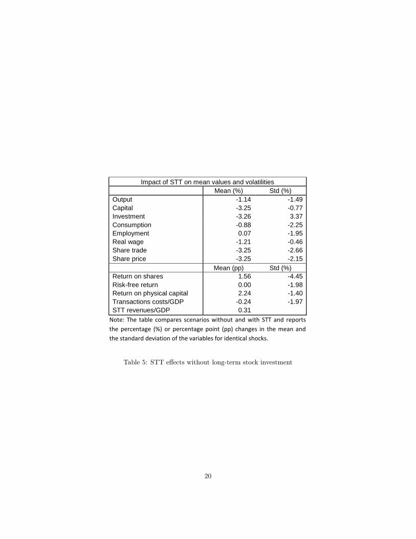
Impact of STT on mean values and volatilitiesMean (%) Std (%)
Output 1.14 1.49Capital 3.25 0.77Investment 3.26 3.37Consumption 0.88 2.25Employment 0.07 1.95Real wage 1.21 0.46Share trade 3.25 2.66Share price 3.25 2.15
Mean (pp) Std (%)Return on shares 1.56 4.45Riskfree return 0.00 1.98Return on physical capital 2.24 1.40Transactions costs/GDP 0.24 1.97STT revenues/GDP 0.31
Note: The table compares scenarios without and with STT and reportsthe percentage (%) or percentage point (pp) changes in the mean andthe standard deviation of the variables for identical shocks.
Table 5: STT e¤ects without long-term stock investment
20
Varying the share of long-term versus short-term investment provides thefollowing results: First, the tax revenue raised increases with falling �, becausehigher short-term investment and trading volumes increase the tax base. Sec-ond, the STT�s negative impact on mean levels of investment, wages, consump-tion and output that is associated with rising capital costs increases substantiallywhen the share of long-term stock holding decreases as a decline in � raises theshare of equity subject to the STT.5
5.3 Alternative degrees of noise trading
A second robustness check concerns the importance of noise trading, keepingthe STT rate constant. Based on empirical studies, the benchmark parameter-isation assumes half of the traders to have noisy expectations. Table 6 and 7report results for noise-trader shares of 25% (sn = 0:25) and 75% (sn = 0:75)respectively. Comparison of the tables shows the long-run behaviour ("mean")of macroeconomic and �nancial variables to be independent of the share ofnoise traders. The STT-related reduction in the volatility of �nancial and realvariables (with the exception of employment) increases with the share of noisetraders, because the relative importance of noise shocks for economic �uctua-tions increases with the share of noise traders. The stabilising impact of anSTT reducing the transmission of noisy expectations into actual trade and realvariables increases in this context.
5.4 The impact on the costs of capital
Absent empirical evidence on the impact of a broad-based STT, we have to relyon model comparison to assess the plausibility of our results. The plausibilitycheck is particularly relevant with respect to the results for the cost of capitalas the STT-related increase of the cost of capital is generally seen and used asthe main argument against the tax.For a robustness check across models we compare the cost-of-capital result
of our benchmark model with a simpler model structure. The simpler general-equilibrium model has only one type of households, i.e. no separate traders, andno �nancing constraint on �rms. In the simpler model, since all shares are heldby households, it can be assumed that �rms maximise the after-tax share valuefor households. This acts like a tax on dividends.
5One can also perform a similar exercise that keeps not the STT rate, but the STT revenueconstant. In this case the e¤ect on the real economy is very similar across di¤erent valuesof �. The intuition is that when the share of assets owned by traders, 1 � �, increases, asmaller tax rate su¢ ces to raise the same revenue. The fact that a larger tax base reducesthe tax rate necessary to raise a certain tax revenue decreases the negative impact of the STTon real variables. On the other hand, an increase in 1 � � subjects a larger share of equityin the economy to taxation , which increases the impact of a given tax rate on capital costsand trading volumes. The two e¤ects are nearly o¤setting in our model, which brings theaggregate e¤ect of varying � close to zero.
21

Impact of STT on mean values and volatilitiesMean (%) Std (%)
Output 0.19 0.43Capital 0.43 0.15Investment 0.42 1.96Consumption 0.02 1.54Employment 0.06 6.40Real wage 0.14 0.03Share trade 8.42 12.36Share price 8.40 1.62
Mean (pp) Std (%)Return on shares 1.25 8.61Riskfree return 0.00 7.57Return on physical capital 0.04 0.47Transactions costs/GDP 0.06 2.96STT revenues/GDP 0.09
Note: The table compares scenarios without and with STT and reportsthe percentage (%) or percentage point (pp) changes in the mean andthe standard deviation of the variables for identical shocks.
Table 6: STT e¤ects with lower share of noise traders
22

Impact of STT on mean values and volatilitiesMean (%) Std (%)
Output 0.19 2.50Capital 0.43 0.05Investment 0.42 4.51Consumption 0.02 4.76Employment 0.06 7.81Real wage 0.14 0.49Share trade 8.40 11.91Share price 8.40 1.89
Mean (pp) Std (%)Return on shares 1.25 8.61Riskfree return 0.00 7.59Return on physical capital 0.04 2.84Transactions costs/GDP 0.06 2.91STT revenues/GDP 0.09
Note: The table compares scenarios without and with STT and reportsthe percentage (%) or percentage point (pp) changes in the mean andthe standard deviation of the variables for identical shocks.
Table 7: STT e¤ects with higher share of noise traders
23

The STT�s e¤ect in this structure is to increase the compound discountfactor, which discourages savings. Given a decline in savings, borrowing costsfor �rms will increase. For more details, the structure of the simpler modelis attached in appendix B. Levying 0.1% of GDP tax revenue with an STTincreases the cost of capital in the simpler model by annualised 4 basis points,while in the benchmark model the tax increases the cost of capital by 4-5 basispoints.The equation describing the cost of capital in the simpler model is identical
to the formula used by Matheson (2011) to asses the impact of the STT in apartial-equilibrium framework, which captures the STT as a tax on dividends.Abstracting from the corporate income tax and from any source of �nancingalternative to shares, as does Matheson (2011), and hence considering the largestpossible tax base, the tax rate that raises 0.1% of GDP tax revenue when paidonce per quarter is 1 basis point. According to Matheson�s (2011) formula, thisrate of 1 basis point implies an annual increase in capital costs by 4 basis points,which is identical to what the simple general-equilibrium model suggests.
6 Conclusions
To the best of our knowledge, very little theoretical work has been done to assessthe impact of an STT on the real economy. The existing papers that analyseSTTs in the presence of non-fundamental volatility (noise trading) limit them-selves to partial equilibrium analysis and tend to restrict focus to the �nancialmarket. Only Xu (2009) studies the impact of a transaction tax in a general-equilibrium framework with noise traders. Xu (2009) focuses on foreign-currencytransactions, however, as opposed to the STT on stock trading in this paper,and does not include a capital-cost channel for the transmission of taxation toreal economy variables.Similarly, model-based (partial-equilibrium) assessments of the impact of an
STT on equity prices and the cost of capital are scarce. Matheson (2011) usesa simple formula to assess the STT�s e¤ect on equity prices for given interestrates and dividends.In constrast, our model integrates the STT in a coherent general-equilibrium
framework with a �nancing constraint for �rms as link between equity prices and�rms�investment decisions. The approach captures the STT�s long-run impacton equity prices and economic aggregates and creates a link between varia-tions in after-tax stock returns and variations in the cost of capital. Discussingthe STT in a general-equilibrium model allows to analyse the STT�s macro-economic impact, distinguish the relevant transmission channels and assess therobustness of results with respect to �nancial market and real economy charac-teristics. Contrary to partial-equilibrium models (e.g., Kupiec, 1996; Song andZhang, 2005) the general-equilibrium approach captures feedback e¤ects accrossdi¤erent markets and over time.The main conclusions from simulations with the benchmark model are that
a transaction tax generating tax revenue of 0.1% of GDP would (1) increase
24
capital costs by 4-5 basis points, implying a long-term 0.4% decline in the capitalstock and a 0.2% decline in real GDP, and (2) reduce the volatility of physicalinvestment and output by 4% and 1% respectively. The estimate for the capital-cost e¤ect are similar to results from a simpler general-equilibrium model thatestablishes the same link between the STT and capital costs as Matheson (2011).The capital-cost e¤ect operates through the �rms��nancing constraint, wherethe value of equity constrains the possibility of physical investment.Increasing the share of noise traders increases the volatility-dampening im-
pact of the STT in our model and does not a¤ect long-term levels of real and�nancial variables. As the STT targets short-term transactions, increasing theshare of long-term equity holding dampens the negative impact of the tax oncapital costs, investment and output levels at constant tax rates. Real e¤ectsare independent of the share of long-term equity holding if the STT is �xedin terms of tax revenue, however, because the e¤ects of smaller tax bases andhigher required tax rates o¤set each other in this case.The STT dampens the �uctuation of �nancial and real variables in response
to non-fundamental (here, noise) and fundamental (here, TFP) shocks. Giventhat the STT is introduced in a setting with additional frictions, hence theenvironment is not �rst best, the welfare e¤ect of the STT-related dampeningof the share price response to TFP shocks is not unambigous. In an environmentwith �nancial and/or real frictions, adding a distortionary tax can in principlebe second best.Due to the di¢ culties of modelling �nancial markets in DSGE models, sev-
eral elements of the policy debate have not been adressed in this paper: First,the model assumes the STT to be e¤ectively implementable and enforceable.It does not include a market for �nancial derivatives or a distinction betweenprimary and secondary markets. Consequently, the model is silent about �-nancial derivatives and their treatment. It is also silent about the impact ofmarket structure in the �nancial sector on STT e¤ects, which is the key themeof, e.g., Pellizzari and Westerho¤ (2009) and Westerho¤ and Dieci (2006). As itcontains distinct assets (corporate equity, government bonds, loans), the modelcould, however, be used to assess spillover e¤ects of selective versus uniformSTT application across equity and debt markets.Second, using a closed-economy model, which can also be understood as
one-region global model, excludes tax avoidance through cross-border capitalmobility. Addressing this issue in an open-economy framework would pose chal-lenges beyond the current state of the art. Tax avoidance should, in general,reduce STT revenues and the impact of the tax on �nancial and real economicvariables alike. At the same time, broad-based STT introduction might itselftrigger non-trivial changes in the structure of �nancial markets (e.g., new �nan-cial products) with consequences that are di¢ cult or impossible to project.
25

References
[1] Baker, Malcolm, Jeremy Stein and Je¤rey Wurgler (2003): "When Doesthe Market Matter? Stock Prices and the Investment of Equity-DependentFirms," Quarterly Journal of Economics, Vol. 118, 969-1006.
[2] Baltagi, Badi, Dong Li and Qi Li (2006): "Transaction Tax and Stock Mar-ket Behaviour: Evidence from an Emerging Market," Empirical Economics,Vol. 31, 393-408.
[3] Barro, Robert (1990): "The Stock Market and Investment," Review ofFinancial Studies, Vol. 3, 115-131.
[4] Bond, Stephen, Mike Hawkins, and Alexander Klemm (2004): "StampDuty on Shares and its E¤ect on Share Prices," Institute for Fiscal StudiesWP 04/11.
[5] Bond, Philip, Alex Edmans and Itay Goldstein (2011): "The Real E¤ectsof Financial Markets," NBER WP 17719.
[6] Cheung, Yin-Wong, Menzie Chinn and Ian Marsh (2004): "How Do UK-Based Foreign Exchange Dealers Think Their Market Operates?" Interna-tional Journal of Finance and Economics, Vol. 9, 289-306.
[7] Christiano, Lawrence and Jonas Fisher (1995): "Tobin�s Q and Asset Re-turns: Implications for Business Cycle Analysis," NBER WP 5292.
[8] Christiano, Lawrence, Roberto Motto and Massimo Rostagno (2010): "Fi-nancial Factors in Economic Fluctuations," ECB WP 1192.
[9] De Long, Bradford, Andrei Shleifer, Lawrence Summers and Robert Wald-mann (1990): "Noise Trader Risk in Financial Markets," Journal of Polit-ical Economy, Vol. 98, 703-38.
[10] Demary, Markus (2006): "Transaction Taxes, Traders�Behavior and Ex-change Rate Risks," Christian-Albrechts-University of Kiel Department ofEconomics WP 2006-14.
[11] Demary, Markus (2010): "Transaction Taxes and Traders with Heteroge-neous Investment Horizons in an Agent-Based Financial Market Model,"Economics - The Open-Access, Open-Assessment E-Journal, Vol. 4, 1-44.
[12] Fazzari, Steven, Glenn Hubbard and Bruce Petersen (1988): "FinancingConstraints and Corporate Investment," Brookings Papers on EconomicActivity, Vol. 19, 141-206.
[13] Habermeier, Karl and Andrei Kirilenko (2003): "Securities TransactionTaxes and Financial Markets," IMF Sta¤ Papers, Vol. 50, 165-80.
26
[14] Hanke, Michael, Juergen Huber, Michael Kirchler and Matthias Sutter(2010), "The Economic Consequences of a Tobin Tax - An Experimen-tal Analysis," Journal of Economic Behavior and Organization, Vol. 74,58-71.
[15] Hau, Harald (2006): "The Role of Transaction Costs for Financial Volatil-ity: Evidence from the Paris Bourse," Journal of the European EconomicAssociation, Vol. 4, 862-90.
[16] Hemmelgarn, Thomas and Gaetan Nicodeme (2010): "The 2008 FinancialCrisis and Taxation Policy," CEPR DP 7666.
[17] IMF (2010): "A Fair and Substantial Contribution by the Financial Sector:Final Report for the G-20," IMF, Washington, D.C.
[18] Jones, Charles and Paul Seguin (1997): "Transaction Costs and PriceVolatility: Evidence from Commission Deregulation," American EconomicReview, Vol. 87, 728-37.
[19] Keen, Michael (2011): "Rethinking the Taxation of the Financial Sector,"CESifo Economic Studies, Vol. 57, 1-24.
[20] Kirchler, Michael, Juergen Huber and Daniel Kleinlercher (2011): "Mar-ket Microstructure Matters When Imposing a Tobin Tax �Evidence fromLaboratory Experiments," Journal of Economic Behavior and Organization(forthcoming).
[21] Kupiec, Paul (1991): "Stock Market Volatility in OECD Countries: RecentTrends, Consequences for the Real Economy, and Proposals for Reform,"OECD Economic Studies, Vol. 17, 31-54.
[22] Kupiec, Paul (1996): "Noise Traders, Excess Volatility and a SecuritiesTransaction Tax," Journal of Financial Services Research, Vol. 10, 115-29.
[23] Mannaro, Katiuscia, Michele Marchesi and Alessio Setzu (2008): "Usingan Arti�cial Financial Market for Assessing the Impact of Tobin-like Trans-action Taxes," Journal of Economic Behavior and Organization, Vol. 67,445-62.
[24] Matheson, Thornton (2011): "Taxing Financial Transactions: Issues andEvidence," IMF Working Paper 11/54.
[25] Menkho¤, Lukas (2001): "Short-Term Horizons in Foreign Exchange? Sur-vey Evidence from Dealers and Fund Managers," Kyklos, Vol. 54, 27-47.
[26] Menkho¤, Lukas and Mark Taylor (2007): "The Obstinate Passion of For-eign Exchange Professionals: Technical Analysis," Journal of EconomicLiterature, Vol. 45, 936-972.
[27] Miller, Merton (1988): "The Modigliani-Miller Propositions After ThirtyYears," Journal of Economic Perspectives, Vol. 2, 99-120.
27

[28] Morck, Randall, Andrei Shleifer and Robert Vishny (1990): "The StockMarket and Investment: Is the Market a Sideshow?," Brookings Papers onEconomic Activity, Vol. 21, 157-216.
[29] Oberlechner, Thomas (2001): "Importance of Technical and FundamentalAnalysis in the European Foreign Exchange Market," International Journalof Finance and Economics, Vol. 6, 81-93.
[30] Pellizzari, Paolo and Frank Westerho¤ (2009): "Some E¤ects of Transac-tion Taxes Under Di¤erent Microstructures," Journal of Economic Behaviorand Organization, Vol. 72, 850-63.
[31] Pierdzioch, Christian (2005): "Noise Trading and Delayed Exchange RateOvershooting," Journal of Economic Behavior and Organization, Vol. 58,133-156.
[32] Qi, Chen, Itay Goldstein and Wei Jiang (2008): "Price Informativeness andInvestment Sensitivity to Stock Prices," Review of Financial Studies, Vol.20, 619-650.
[33] Schulmeister, Stephan, Margit Schratzenstaller, Oliver Picek (2008): "AGeneral Financial Transaction Tax: Motives, Revenues, Feasibility andE¤ects," Oesterreichisches Institut fuer Wirtschaftsforschung WP 3/2008.
[34] Schwert, William and Paul Seguin (1993): "Securities Transaction Taxes:An Overview of Costs, Bene�ts and Unresolved Questions," Financial An-alysts Journal, Vol. 49, 27-35.
[35] Shackelford, Douglas, Daniel Shaviro, and Joel Slemrod (2010): "Taxationand the Financial Sector," New York University Law and Economics WP224.
[36] Shleifer, Andrei and Lawrence Summers (1990): "The Noise Trader Ap-proach to Finance," Journal of Economic Perspectives, Vol. 4, 19-33.
[37] Song, Frank and Junxi Zhang (2005): "Securities Transaction Tax andMarket Volatility," The Economic Journal, Vol. 115, 1103-20.
[38] Stiglitz, Joseph (1989): "Using Tax Policy to Curb Speculative Short-TermTrading," Journal of Financial Services Research, Vol. 3, 101-15.
[39] Summers, Lawrence and Victoria Summers (1989): "When Financial Mar-kets Work Too Well: A Cautious Case For a Securities Transaction Tax,"Journal of Financial Services Research, Vol. 3, 261-86.
[40] Tirole, Jean (2006): The Theory of Corporate Finance. Princeton: Prince-ton University Press.
28
[41] Westerho¤, Frank and Roberto Dieci (2006): "The E¤ectiveness of Keynes-Tobin Transaction Taxes When Heterogeneous Agents Can Trade in Dif-ferent Markets: A Behavioral Finance Approach," Journal of EconomicDynamics and Control, Vol. 30, 293-322.
[42] Xu, Juanyi (2010): "Noise Traders, Exchange Rate Disconnect Puzzle, andthe Tobin Tax," Journal of International Money and Finance, Vol. 29, 336-57.
A Equations in the simulated benchmark model
A.1 Households
!L�t Clt =
�1� � l
�Wt
�lt = 1=Clt
�lt = �RtEt�lt+1
1 = �Et
"�lt+1
�lt
�P shllt+1 +DIVt+1
P shllt
�#
A.2 Financial traders
CTt = (1� sn)CT;It + snC
T;Nt
�Tt = sn=CT;Nt + (1� sn) =CT;It
aTt = (1� sn) aT;It + sna
T;Nt
ENt Rsht+1 = EtR
sht+1 + �t
Etc+ �STT
CT;It+1
aT;It = EtRsht+1 �RtCT;It+1
ENtc+ �STT
CT;Nt+1
aT;Nt = ENtRsht+1 �RtCT;Nt+1
CT;It = �w +�P sht +DIVt
�aT;It�1 �Rt�1P sht�1a
T;It�1
�c+ �STT
2P sht�1
�aT;It�1
�2CT;Nt = �w +
�P sht +DIVt
�aT;Nt�1 �Rt�1P sht�1a
T;Nt�1
�c+ �STT
2P sht�1
�aT;Nt�1
�2
29
A.3 Firms
Yt = At (Kt�1)1��
(slLt)�
Kt = (1� �)Kt�1 + It
DIVt � (1� � c) (Yt �WtslLt) + �c�Kt�1 � It
It = ��Et
"�lt+1
�lt
��P shllt+1 + (1� �)P sht+1
�#
�YtslLt
=Wt
Qt = �Et�lt+1
�lt
�(1� � c) (1� �) Yt+1
Kt+ � c� + (1� �)Qt+1
�Qt = 1 + �t
A.4 Government
BGt =Rt = BGt�1 +Gt � � lWtslLt � slT lst � � c (Yt �WtslLt) + �c�Kt�1
� (1� sl)�STT
2P sht�1
�(1� sn)
�aT;It�1
�2+ sn
�aT;Nt�1
�2�
T lst = T lst�1 + �Tls
�BGtYt
�BY�
A.5 Aggregation and equilibrium
alt = �=sl
aTt = (1� �) = (1� sl)at = sla
lt + (1� sl) aTt = 1
Blt =1
sl
�BGtRt
+ (1� sl)P sht aTt�
Ct = slClt + (1� sl)CTt
Blt =BGt + (1� sl)P sht aTt
sl
Yt = Ct+Gt+ It+(1� sl)c
2P sht�1
�(1� sn)
�aT;It�1
�2+ sn
�aT;Nt�1
�2�� (1� sl) �w
A.6 Exogenous processes
lnAt = (1� �a) ln �A+ � lnAt�1 + "at�t = "
�t
30

B Simple general-equilibrium model
This appendix outlines the simple model udes for comparison in section 5.4.Unless stated otherwise, notation is as in the benchmark model.
B.1 Households
There is a representative household that maximises:
maxCt;Nt;at
E0
1Xt=0
�t�lnCt �
!
1 + �L1+�t
�subject to the budget constraint:
Ct +Bt + Psht St = WtNt + (1 + rt�1)Bt�1
+�1� �STT
� �P sht +DIVt
�St�1 � T lst
B.2 Firms
The �rms maximise the present value of future dividend �ows discounted at thestochastic discount factor DFt;t+i (to be de�ned below) of their owners:
maxKt+i;Nt+i
Et
1Xi=0
DFt;t+i [DIVt+i(Kt+i; Lt+i)]
Dividends equal corporate income net of the wage bill, capital depreciation andinvestment:
DIVt(Kt; Lt) � (1� � c) (Yt �WtLt) + �c�Kt � It
Maximising the steam of dividends is subject to the constraints:
Yt = AtL�t K
1��t
Kt = (1� �)Kt�1 + It
which describe the production technology and capital accumulation.
B.3 Government
The government budget constraint is:
BGt = (1 + rt�1)BGt�1 +Gt � � c (Yt �WtLt � �Kt�1)� �STTP sht St � T lst
31

B.4 Market clearing
In equilibrium, the transversality condition holds and all markets clear. For thegoods market this implies:
Yt = Ct + It +Gt
Equilibrium in the capital market implies equality between domestic savingsand capital investment. The number of stocks de�ning �rm ownership is keptconstant at St = 1.
B.5 First order conditions
The households�FOC of the optimisation are:
�t = 1=Ct
!L�t =Wt�t
1 = ��t+1�t
(1 + rt)
P sht = ��t+1�t
�1� �STT
� �P sht+1 +DIVt+1
�The iteration of the FOC for capital investment gives an expression for currentshare value as the discounted sum of future after-tax dividends:
P sht =1Xi=1
�i�t+i�t
�1� �STT
�iDIVt+i
The �rm maximises the after-tax share value of the owners, so that the stochasticdiscount factor can be de�ned as:
DFt;t+i � �i�t+1+i�t
�1� �STT
�iOptimisation of the share value gives FOCs for the optimal level of employmentand capital:
�YtLt=Wt
F 0 (Kt) � (1� �)YtKt
F 0 (Kt) =1 + � c� + � �t+1�t
�1� �STT
�(1� �)
1� � cHence, the STT directly enters the �rms�FOC for investment.In steady state �, so that the FOC for investment involving the cost of capital
becomes:
F 0 (K) =1� � c� � �
�1� �STT
�(1� �)
1� � c
32

Noting that in the steady state � = 1= (1 + r) and assuming � c = 0 gives:
F 0 (K) = 1��1� �STT
�(1� �)
1 + r
which corresponds to the formula A.16 in Matheson (2011) with �STT = T=N ,where T is the tax rate and N is the lenght of the time interval. In our quarterlymodel, N = 0:25. Interest rates, discount rates and depreciation rates of ourmodel also have to be annualised for a comparison with Matheson (2011).
33