Embed Size (px)
Citation preview

THE HOPF BIFURCATION AND ITS APPLICATIONS
SECTION 9
BIFURCATIONS IN FLUID DYNAMICS AND
THE PROBLEM OF TURBULENCE
285
This section shows how the results of Sections 8 and
8A can be used to establish the bifurcation theorem for the
Navier-Stokes equations. Alternatively, although conceptually
harder (in our opinion) methods are described in Sections 9A,
9B and Sattinger [5] and Joseph and Sattinger [1].
The new proof of the bifurcation theorems using the
center manifold theory as given in Section 8 allow one to de
duce the resul~s very simply for the Navier-Stokes equations
with a minimum of technical difficulties. This includes all
types of bifurcations, including the bifurcation to invariant
tori as in Section 6 or directly as in Jost and Zehnder [1].
All we need to do is verify that the semiflow of the Navier
Stokes equations is smooth (in the sense of Section 8A) i the
rest is then automatic since the center manifold theorem im
mediately reduces us to the finite dimensional case (see

286 THE HOPF BIFURCATION AND ITS APPLICATION
Section 8 for details). We note that already in Ruelle-
Takens [1] there is a simple proof of the now classical re-
sults of Velte [1] on stationary bifurcations in the flow
between rotating cylinders from Couette flow to Taylor cells.
The first part of this section therefore is devoted to
proving that the semiflow of the Navier-Stokes equations is
smooth. We use the technique of Dorroh-Marsden [1] (see Sec-
tion 8A) to do this.
This guarantees then, that the same results as given
in the finite dimensional case in earlier sections, including
the stability calculations hold without change.
The second part of the section briefly describes the
Ruelle-Takens picture of turbulence. This picture is still
conjectural, but seems to be gaining increased acceptance as
time goes on, at least for describing certain types of tur-
bulence. The relationship with the global regularity (or
"all time") problem in fluid mechanics is briefly discussed.
Statement of the Smoothness Theorem.
Before writing down the smoothness theorem, let us re-
call the equations we are dealing with. For homogeneous in-
compressible viscous fluids, the classical Navier-Stokes equa-
tions are, as in Section 1,
3vat + (v·V)v - v~v = -grad p + bt , bt
external force
(NS) 1diV v
v = 0
= 0
on 3M (or prescribed on M, possibly dependingon a parameter ~)
Here M is a compact Riemannian manifold with smooth boundary

THE HOPF BIFURCATION AND ITS APPLICATIONS
3M, usually an open set in R3 .
287
The Euler equations are obtained by supposing v 0
and changing the boundary condition to vi 13M:
I3v + (v.\i)v -grad p + b t3t
(E)
1div v 0
vii 3M
The pressure p(t,x) is to be determined from the in-
compressibility condition in these equations.
The Euler equations are a singular limit of the Navier-
Stokes equations. Taking the limit v + 0 is very subtle and
is the subject of much recent work. The sudden disappearance
of the highest order term and the associated sudden change in
boundary conditions is the source of the difficulties and is
the reason why boundary layer theory and turbulence theory
are so difficult. This point will be remarked on later.
Note that Euler equations are reversible in the sense
that if we can solve them for all sets of initial data and
for t ~ 0, then we can also solve them for t < O. This is
hecause if
t < o.
is a solution, then so is wt -v_ t '
For s > 0 an integer and I < P < 00, let wS'P de-
note the Sobolev space of functions (or vector functions) on
M ~.,hose derivatives up to order s are in
of describing Ws,p is to complete the COO
the norm
II f II s,p L IIDafll LO.::.a.::.s p
Lp ; another way
functions f in

288 THE HOPF BIFURCATION AND ITS APPLICATIONS
where Daf is the a th total derivative of f. Details on
Sobolev spaces can be found in Friedman [1].
We point out that in the non-compact case one must deal
seriously with the asymptotic conditions and many of the re
sults we discuss are not known in that case (see Cantor [1],
and McCracken [2] however).
The following result is a special case of a general
result proved in Morrey [1]. For a direct proof in this case,
see Bourguignon and Brezis [1].
(9.1) Lemma. Hodge Decomposition): Let M be as
above. Let X be a ws,p vector field on M, s > 0, p > 1.
Then X has a unique decomposition as follows:
X = Y + grad p
where div Y = 0 and yl laM. It is also true that Y E ws,p
and p E ws+l,p.
div X
Let wS'P = {vector fields X on Mix E wS,P,
o and xl laM}. By the Hodge theorem, there is a map
(E)
P: ws,p + Ws,p via X ~ Y. The problem of solving the Euler
equations now becomes that of finding v t E ws+l,p such that
dVtdt + P«vt·V)vt ) = 0
s > ~ the p_roduct of two ws,pp'(plus initial data).
functions is Ws,p so
If
(v·V)v is in ws,p if v E ws+l,p.
This kind of equation is thus an evolution equation on wS'P
as in Section 8A.
Let

THE HOPF BIFURCATION AND ITS APPLICATIONS 289
ws,p {vector fields v on Mlv is of class
° ~ls,P , div v = ° and v = ° on 3M}.
If s = ° this actually makes. sense and the space is
written J (see Ladyzhenskaya [1]).p
The Navier-Stokes equations can be written: find
(NS)
such that
dVt - vP~v + P(vt·V)vt = °
dt t
again an evolution equation in W~'p. In the terminology of
Section 8A, the Banach space X here is wO,p
°y = W2 ,p. The bifurcation parameter is often
°Reynolds number.
J p and
11 = l/v, the
The case p ~ 2 is quite difficult and won't be dealt
with here, although it is very important. If p = 2 one
generally writes
-s 2llil ' , etc.
(9.2) Theorem. The Navier-Stokes equations in dimen
sion 2 or 3 define a smooth local semiflow on H~ C HO = J.
This semiflow satisfies conditions 8.1, 8.2, and the
smoothness in 8.3 of Section 8, so the Hopf theorems apply.
(The rest of the hypotheses in 8.3 and 8.4 depend on the
particular problem at hand and must be verified by calcula-
tion. )
In other words, the technical difficulties related to
the fact that we have partial rather than ordinary differen-
tial equations are automatically taken care of.
(9.3) Remarks. 1. If the boundaries are moving and

290 THE HOPF BIFURCATION AND ITS APPLICATIONS
speed is part of the bifurcation parameter ~, the same re
sult holds by a similar proof. This occurs in, for instance
the Taylor problem.
2. The above theorem is implicit in the works of many
authors. For example, D. Henry has informed us that he has
obtained it in the context of Kato-Fujita. It has been
proved by many authors in dimension 2 (e.g. Prodi). The
first explicit demonstration we have seen is that of Iooss
[3,5] •
3. For the case p I 2 see McCracken [2].
4. This smoothness for the Navier-Stokes semiflow is
probably false for the Euler equations on HS (see Kato [6],
Ebin-Marsden [1]). Thus it depends crucially on the dissi
pative term. However, miraculously, the flow of the Euler
equations is smooth if one uses Lagrangian coordinates (Ebin
Marsden [1]).
We could use Lagrangian coordinates to prove our re
sults for the Navier-Stokes equations as well, but it is
simpler to use the present method.
Before proving smoothness we need a local existence
theorem. Since this is readily available in the literature
(Ladyzhenskaya [1]), we shall just sketch the method from a
different point of view. (Cf. Soboleoskii [1].)
Local Existence Theory.
The basic method one can use derives from the use of
integral equations as in the Picard method for ordinary dif
ferential equations. For partial differential equations this
has been exploited by Segal [1], Kato-Jujita [1], Iooss [3,6],

THE HOPF BIFURCATION AND ITS APPLICATIONS 291
Sattinger [2], etc. (See Carroll [1] for general background.)
The following result is a formulation of Weissler [11.
(See Section 9A for a discussion of Iooss' setup.)
First some notation: EO' El , E2 will be three Banach
spaces with norms I I· I 10' 1/· I 11' I I· I 12 , with E2 C El CEO'
with the inclusions dense and continuous. (Some of the
spaces may be equal.) Let etA be a cO linear semigroup
on EO which restricts to a contraction semigroup on E: 2 ·
Assume, for t > 0, tA El->- E
2is a bounded lineare : map
and let its norm be denoted II (t). Our first assumption is:
AI) For T > 0 assume JT
ll(T)dTo
< co
For the Navier-Stokes equations, A
choose either
vPL'l, and we can
(See Yosida [1].)
(i) HI -2EO = J
2, lEI = and IE H
O2or (E) EO = lEI = li- l / 2 = completion of J with the
-1/4 -1 (-vPL'l) 1/2.norm 11(-vpL'l) uil L , E2 = H = domain of2
The case (ii) is that of Kato-Fujita [1].
The fact that AI) holds is due to the fact that
is a negative self adjoint operator on J with domain
(Ladyzhenska~a [1]); generates an analytic semigroup, so the
e tA -2 /norm of from HO
to J 2 is ~ C t.
However we have the Sobolev inequality {derived most easily
from the general Sobolev-Nirenberg-Gagliardo inequality from
Nirenberg [1]:
where

292 THE HOPF BIFURCATION AND ITS APPLICATIONS
1P
i + a(l _ ~) + (l-a) 1n r n q'
(if m - j - n is an integer > 1, a = 1 is not allowed)},r
that
so we can choose ~(t) < C/It, so Al) holds. Similarly
in case (ii) one finds ~(t) = C/t3/ 4 (Kato-Fujita [1]).
As for the nonlinear terms, assume
A2) Jt
: E2 + El is a semi-Lipschitz map (i.e.,
Lipschitz on bounded sets), locally uniformly in t with
J t (¢) continuous in (t,¢). We can suppose Jt(O) = 0 for
simplici ty.
Consider the "formal" differential equation
~ = A¢ + J (¢)dt t
in integral equation form (see e.g., Segal [1])
(9.1)
(9.2)
where t > to.
difficulties. )
(Adding an inhomogeneous term causes no real
(9.4) Theorem. Under assumptions Al) and A2), the
equation (9.2) defines a unique local semiflow (i.e., evolu
tion system) ~ E2 (in the sense of Section 8A) with
W(t,tO): E2 + E2 locally uniformly Lipschitz, varying con
tinuously in t.
Proof. The proof proceeds by the usual contraction

THE HOPF BIFURCATION AND ITS APPLICATIONS 293
mapping argument as for ordinary differential equations (see
Lang [1]) : Pick o < a < a, let Ka (t) be the Lipschitz0
constant of J t from 1E 2 to lEI on B the a ball abouta
and pick T such that
r- t aO( 0 !l (T)dT) ( sup K (T» < 1 - - (9.3)
0 TE[tO,T] a a
withto[O,T]
and let M be the complete metric space
sup j1<I>(t)-'JI(t)j12tE[tO,T]
Define 5': M ->- M by
Now choose ¢ EB
cOa O
of maps <I> of
and metric
d(¢,'JI)
(t-tO)A5'<1> (t) = e ¢
From the definitions and
Jt (t-T)A
+ e JT(¢(T»dTto
(9.3) we have two key estimates:
first
rto
!l(t-T)K (T)·adTa
= a
(9.4 )
(remember JT(O) = 0 here), which shows ~ maps M to M
and, in the same way
.ad(~¢, 5''JI) 2 (1 - ~)d(¢,'JI)
a(9.5 )
which shows ~ is a contraction.
The result now follows easily. []
(9.5) Exercises. 1. Show that W(t,tO) has E2
Lipschitz constant given by a/aO. Verify that W(t,s)W(s,tO)
W(t,tO)·

294
and
THE HOPF BIFURCATION AND ITS APPLICATIONS
2. If ¢t is a maximal solution of (9.2) on [O,T)
T < 00, show lim sup I I¢ / /2 = 00; i.e., verify the continuat .... T t
tion assumption B.2.
3. Use the Sobolev inequalities to verify that
P«u·V)u) satisfies the hypotheses in case (i)
above. For case (ii), see Kato-Fujita [1].
Next we want to see that we actually have a solution
of the differential equation. Make
A3) Assume that the domain of A as an operator in
(9.6) Theorem. If AI), A2) and A3) hold, then any
solution of (9.2) solves (9.1) as an evolution system in lEo
with domain D = 1E2
; (in the terminology of Section BA,
W(t,tO) is the (time dependent) local flow of the operator
X(¢) = A(¢) + J t (¢), mapping E2 to lEO). Solutions of
(9.2) in E 2 are unique.
Proof. Let ¢ E E2 and ¢(t) = W(t,tO
)¢ E 1E2
be
the solution of (9.2), so taking to = a for simplicity,
It is easy to verify that
~{¢(t+h)-¢(t)} = ~{ehA¢(t)_¢(t)} - Jt(¢(t»
t+h+! I {e(t+h-T)AJ (¢(T»-Jt(¢(t»}dT
h t T
writing
(9.6 )
THE HOPF BIFURCATION AND ITS APPLICATIONS 295
e(t+h-T)AJT(¢(T» - Jt(¢(t»
e(t+h-T)A[JT(¢(T»-Jt(¢(t»] + et+h-TJt(¢(t»-Jt~(t»
one sees that the last term of (9.6) ~ a as h ~ a in 12:1
and hence in ~o. The first term of (9.6) tend to
A(¢(t» - Jt(¢(t» in ~O as h ~ a since ¢(t) E ~2' the
domain of A. []
Thus we can conclude that the Navier-Stokes equations
define a local semiflow on
tends to a local semiflow on
and that this semi flow ex-
(via the integral equation).
Smoothness.
(9.7) Theorem. Let Al), A2) and A3) hold and assume
A4)00
J t : ~2 ~ ~l is C with derivatives depending
continuously on t.
Then the semiflow defined by equations (9.1) on ~2
is a COO semiflow on E ; i.e., each W(t,tO
)2 --
00
is C with
derivatives varying continuously in t in the strong topology
(see Section 8).
Proof. We verify the hypotheses of (8A.31). Here we
take X = EO and Y = E2
, with D = Y. Certainly a) holds
by hypothesis. Since Z(¢1'¢2) is the same type of operator
as considered above, 9.4 shows b) holds. c ' ) holds by the
E2
Lipschitzness of W(t,tO) proven in (9.4) and d) is
clear.
Hence W(t,tO): E2 ~ ~2 is Gateaux differentiable.

296 THE HOPF BIFURCATION AND ITS APPLICATIONS
The procedure can be iterated. The same argument ap-
plies to the semiflow
on iE2
-+ iE 2 .
Hence W is cl (see (8A.32», and by induction is
COO. D
In the context of equation (9.1) the full power of the
machinery in Section 8A; in particular the delicate results
on time dependent evolution equations are not needed. One can
in fact directly prove (9.7) by the same method as (8A.3l).
However it seems desirable to derive these types of results
from a unified point of view.
(9.8) Problem. Assume, in addition that
AS) A generates an analytic semigroup.
Show that for t > a and ¢ EEl' ¢(t) lies in the domain
of every power of A and that ¢(t) is a COO function of
t for t > O. (Hint. Use (8A.33». Also establish smooth-
ness in v if A is replaced by vA (see remarks follow-
ing (8A. 33) ) •
A more careful analysis actually shows that W(t,tO)
are COO maps on HI in the context of the Navier-Stokes
equation (i.e., without assuming A3». See Weissler [1].
Thus all the requisite smoothness is established for
the Navier-Stokes equations, so the proof of (9.2) and hence
the bifurcation theorems for those equations is established.

THE HOPF BIFURCATION AND ITS APPLICATIONS
The Problem of Turbulence.
297
We have already seen how bifurcations can lead from
stable fixed points to stable periodic orbits and then to
stable 2-tori. Similarly we can go on to higher dimensional
tori. Ruelle and Takens [1] have argued that in this or
other situations, complicated ("strange") attractors can be
expected and that this lies at the roots of the explanation
of turbulence.
The particular case where tori of increasing dimen~
sion form, the model is a technical improvement over the idea
of E. Hopf [4] wherein turbulence results from a l6ss of
stability through successive branching. It seems however
that strange attractors may form in other cases too, such as
in the Lorenz equations (see Section 4B) [Strictly speaking,
it has only a "strange" invariant set]. This is perfectly
consistent with the general Ruelle-Takens picture, as are
the closely related "snap through" ideas of Joseph and
Sattinger [1].
In the branching process, stable solutions become un
stable, as the Reynolds number is increased. Hence turbu
lence is supposed ~o be a necessary consequence of the equa
tions and in fact of the "generic case" and just represents a
complicated solution. For example in Couette flow as one in
creases the angular velocity ~l of the inner cylinder one
finds a shift from laminar flow to Taylor cells or related
patterns at some bifurcation value of ~l. Eventually turbu
lence sets in. In this scheme, as has been realized for a
long time, one first looks for a stability theorem and for
when stability fails (Hopf [2], Chandresekar [1], Lin [1] etc.).

298 THE HOPF BIFURCATION AND ITS APPLICATIONS
For example, if one stayed closed enough to laminar flow, one
would expect the flow to remain approximately laminar. Serrin
[2] has a theorem of this sort which we present as an illus-
tration:
(9.9) Stability Theorem. Let D C R3 be a bounded
domain and suppose the flow is prescribed on ClD (this
corresponds to having a moving boundary, as in Couette flow).
vLet V = maxI Iv (x) I I, d = diameter of D and v equal the
xED tt>O
viscosity. Then if the Reynolds number R = (Vd/v) ~ 5.71,
is universally L2
Stokes equations.
stable among solutions of the Navier-
Universally L2 stable means that if is any
other solution to the equations and with the same boundary
conditions, then the L2
norm (or energy) of v~ - v~ goes
to zero as t + O.
The proof is really very simple and we recommend read-
ing Serrin [1,2] for the argument. In fact one has local
stability in stronger topologies using Theorem 1.4 of Section
2A and the ideas of Section 8.
Chandresekar [1], Serrin [2], and Velte [3] have analy-
zed criteria of this sort in some detail for Couette flow.
As a special case, we recover something that we ex-
then vV + 0 as t + 00
t
is universally stable.
pect. Namely if on ClM is any solution for v + 0
in L2
norm, since the zero solution
A traditional definition (as in Hopf [2], Landau-

THE HOPF BIFURCATION AND ITS APPLICATIONS 299
Lifschitz [1]) says that turbulence develops when the vector
field
where
can be described as vt(wl' ••. ,wn )
is a quasi-periodic function, i.e., f
f(twl,···,twn )
is periodic
in each coordinate, but the periods are not rationally related.
For example, if the orbits of the v t on the tori given by
the Hopf theorem can be described by spirals with irrationally
related angles, then v t would such a flow.
Considering the above example a bit further, it should
be clear there are many orbits that the vt
could follow
which are qualitatively like the quasi-periodic ones hut
which fail themselves to be quasi-periodic. In fact a small
neighborhood of a quasi-periodic function may fail to contain
many other such functions. One might desire the functions
describing turbulence to contain mos.t functions and not only
a sparse subset. More precisely, say a subset U of a top
ological s~ace S is generic if it is a Baire set (i.e., the
countable intersection of open dense subsets). It seems
reasonable to expect that the functions describing turbulence
should be generic, since turbulence is a common phenomena. and
the equations of flow are never exact. Thus we would want a
theory of turbulence that would not be destroyed by adding on
small perturbations to the equations of motion.
The above sort of reasoning lead Ruelle-Takens [1] to
point out that since quasi-periodic functions are not generic,
it is unlikely they "really" describe turbulence. In its
place, they propose the use of "strange attractors." These
exhibit much of the qualitative behavior one would expect from
"turbulent" solutions to the Navier-Stokes equations and they
are stable under perturbations of the equations; i.e., are

300 THE HOPF BIFURCATION AND ITS APPLICATIONS
"structurally stable".
For an example of a strange attractor, see Smale [1].
Usually strange attractors look like Cantor sets x mani-
folds, at least locally.
Ruelle-Takens [1] have shown that if we define a
strange attractor A to be an attractor which is neither a
closed orbit or a point, and disregarding non-generic pos-
sibilities such as a figure 8 then there are strange attrac
tors on T4 in the sense that a whole open neighborhood of
vector fields has a strange attractor as well.
If the attracting set of the flow, in the space of
vector fields which is generated by Navier-Stokes equations
is strange, then a solution attracted to this set will clearly
behave in a complicated, turhulent manner. While the whole
set is stable, individual points in it are not. Thus (see
Figure 9.1) an attracted orbit is constantly near unstable
(nearly periodic) solutions and gets shifted about the at-
tractor in an aimless manner. Thus we have the following
reasonable definition of turbulence as proposed by Ruelle-
Takens:
nonstationarysolution of the
Navier- Stokesequations
Zstrange attractor
in the space of allvelocity fields
Figure 9.1
THE HOPF BIFURCATION AND ITS APPLICATIONS 301
" •.• the motion of a fluid system is turbulent when
this motion is described by an integral curve of a vector
field x~ which tends to a set A, and A is neither empty
nor a fixed point nor a closed orbit."
One way that turbulent motion can occur on one of the
tori Tk that occurs in the Hopf bifurcation. This takes
place after a finite number of successive bifurcations have
occurred. However as S. Smale and C. Simon pointed out to
us, there may be an infinite number of other qualitative
changes which occur during this onset of turbulence (such as
stable and unstable manifolds intersecting in various ways
etc.). However, it seems that turbulence can occur in other
ways too. For example, in Example 4B.9 (the Lorenz equa
tions), the Hopf bifurcation is subcritical and the strange
attractor may suddenly appear as ~ crosses the critical
value without an oscillation developing first. See Section 12
for a description of the attractor which appears. See also
McLaughlin and Martin [1,2], Guckenheimer and Yorke [1] and
Lanford [2].
In summary then, this view of turbulence may be
phrased as follows. Our solutions for small ~ (= Reynolds
number in many fluid problems) are stahle and as ~ increa
ses, these solutions become unstable at certain critical
values of ~ and the solution falls to a more complicated
stable solution; eventually, after a certain (finite) number
of such bifurcations, the solution falls to a strange attrac
tor (in the space of all time dependent solutions to the prob
lem). Such a solution, which is wandering close to a strange
attractor, is called turbulent.

302 THE HOPF BIFURCATION AND ITS APPLICATIONS
The fall to a strange attractor may occur after a Hopf
bifurcation to an oscillatory solution and then to invariant
tori, or may appear by some other mechanism, such as in the
Lorenz equations as explained above ("snap through turbulence").
Leray [3] has argued that the Navier-Stokes equations
might break down and the solutions fail to be smooth when
turbulence ensues. This idea was amplified when Hopf [3]
in 1950 proved global existence (in time) of weak solutions
to the equations, but not uniqueness. It was speculated that
turbulence occurs when strong changes to weak and uniqueness
is lost. However it is still unknown whether or not this
really can happen (cf. Ladyzhenskaya [1,2].)
The Ruelle-Takens and Leray pictures are in conflict.
Indeed, if strange attractors are the explanation, their at
tractiveness implies that solutions r~main smooth for all t.
Indeed, we know from our work on the Hopf bifucation that
near the stable closed orbit solutions are defined and re
main smooth and unique for all t > 0 (see Section 8 and
also Sattinger [2]). This is already in the range of inter
esting Reynolds numbers where global smoothness isnot implied
by the classical estimates.
It is known that in two dimensions the solutions of
the Euler and Navier-Stokes equations are global in t and
remain smooth. In three dimensions it is unknown and is
called the "global regularity" or "all time" problem.
Recent numberical evidence (see ~am et. al. [1])
suggests that the answer is negative for the Euler equations.
Theoretical investigations, including analysis of the

THE HOPF BIFURCATION AND ITS APPLICATIONS 303
spectra have been inconclusive for the Navier-Stokes equa
tions (see Marsden-Ebin-Fischer [1] and articles by Frisch
and others in Temam et.al. [1]).
We wish to make two points in the way of conjectures:
1. In the Ruelle-Takens picture, global regularity
for all initial data is not an a priori necessity; the basins
of the attractors will determine which solutions are regular
and will guarantee regularity for turbulent solutions (which
is what most people now believe is the case).
2. Global regularity, if true in general, will pro
bably never be proved by making estimates on the equations.
One needs to examine in much more depth the attracting sets
in the infinite dimensional dynamical system of tpe Navier
Stokes equations and to obtain the a priori estimates this
way.
Two Major Open Problems:
(i) identify a ptrange attractor in a specific flow
of the Navier-Stokes equation (e.g, pipe flow, flow behind a
cylinder, etc.).
(ii) link up the ergodic theory on the strange at
tractor, (Bowen-Ruelle [1]) with the statistical theory of
turbulence (the usual reference is Batchellor [1]; however,
the theory is far from understood; some of Hopf's ideas [5]
have been recently developed in work of Chorin, Foias and
others) .

304 THE HOPF BIFURCATION AND ITS APPLICATIONS
SECTION 9A
ON A PAPER OF G. IOOSS
BY G. CHILDS
This paper [3) proves the existence of the Hopf bi-
furcation to a periodic solution from a stationary solution
in certain problems of fluid dynamics. The results are simi
lar to those already described. For instance, in the sub
critical case, the periodic solution is shown to be unstable
in the sense of Lyapunov when the real bifurcation parameter
(Reynold's number) is less than the critical value where the
bifurcation takes place; it is shown to be (exponentially)
stable if this value is greater than the critical value in
the supercritical case.
Iooss, in contrast to the main body of these notes,
makes use of a linear space approach for almost all of what
he does. Specifically, his periodic solution is a continuous
function to elements of a Sobolev space on a fundamental do
main ~ in ~3. However, the implicit function theorem is
extensively used. The three main theorems of the paper will

THE HOPF BIFURCATION AND ITS APPLICATIONS 305
be stated and the proofs will be briefly outlined to illus-
trate this method.
First, we formulate a statement of the problem. Let
I be a closed interval of the real line. Let V(I) be a
neighborhood in iC of this interval. For each A E V (I) ,
LA is a closed, linear operator on a Hilbert space H. The
Also, each LA is m-sectorial with vertex-y A.
family {LA}
[3), p. 375).
is holomorphic of type (A) in V(I) (see Kato
Finally, LA has a compact resolvent in H. Let ~ be the
common domain of the LA. Assume K is a Hilbert space such
that ~ eKe H with continuous inj ections and such thaty t
VU E K, II I (t)ull~ .::. ke A (l+t-a
) IlulIK, 0 .2 a < 1 where
is the holomorphic semi-group generated by -LA. Let
M be a continuous bilinear form: ~ x 9 ->- K. Now we can
state the problem:
auat + LAU - M(U,U) 0
U E CO(O,OO;~) n Cl(O,OO;H) (9A.l)
U(O) = Uo E ~, U(O) = U(T) = U(2T) = ••• for some T > 0
IOOS5 shows that the equation of perturbation (from a sta
tionary solution) for some Navier-Stokes configurations is of
the above form (see also Iooss [5 ) for more details). In
order to find a solution of (9A.l), it is necessary to make some
additional hypotheses. Let sO(A) = sup {Re ~}. Then:sEer (-LA)
(H.l) 3 A neighborhood - (A ) andE R, a left hand Vc c
a right hand neighborhood v+ (I.e) such that s (A ) = 0,o c
A E V- (A ) {A }~ s (A) < 0, A E: v+ (A ) {A }=$- s (A) > O.- -c c 0 c c 0

306 THE HOPF BIFURCATION AND ITS APPLICATIONS
(H.2) The operator LA admits as proper values purec
imaginary numbers ~O = in O and f o' Also, these proper
values are simple. For A E V(A) there exist two analyticc
functions sl and f l E cr(-LA)
spectrum cr(LA) separates into
such that sl (AC
) = sO' The
{-sl} U {-fl } U cr(LA). This
separation gives a decomposition of H into invariant sub-
spaces:
'v'UEH, U=X+Y, X=EAU, Y=PAU;
EA = E(-s ) + E(-fl ), (LA+sl)Ul (A) = 0, (L~+fl)Wl (A) = 0,1
(Ul(A),Wl (A»H = 1, (U l (A),W(O»H = 1. The eigenvectors
Ul(A), UlTAf are a basis for EAH. For A E V(AC)' LAU
~ ('_' )nL(n)u,. U (') (0) (1)LA U + L A A 1 A U + (A-A)U + •.• ;c n=l c c
WI (A) = W(O) + (A-Ac)w(l) + •.. ; sl (A) So + (A-AC
) S (1) +••••
In particular, we have sell = _(L(l)u(O) ,W(O»H' LA +c
sOU ( 0 ) = 0, L~ + f W(0) = 0, (U ( 0 ) W(0) ) = 1. Now, we cancO' H
make the hypothesis:
(H.3) Re(L(l)u(O) ,W(O»H"I- o. By (H.l) this implies
Re sell > O. These hypotheses are just the standard Ones for
the existence of the Hopf bifurcation.
the theorem we also need to know that
For the statement of
Y = YO + iyO.o r 1.
_ (M(O) [U (0) ,L~lM (0) (U (0) ,U (0»] +c
M(O) [U(O) ,(LA +2inol)-lM(U(0) ,u(O»], W(O»H where
c
M(O) (U,V) = M(U,V) + M(V,U).
We now state Iooss'
Theorem 2. If the hypotheses (H.l), (H.2), (H.3), and

THE HOPF BIFURCATION AND ITS APPLICATIONS 307
are satisfied, there is a bifurcation to a non-
aArg
The solutionA E V-(A ).c
is unique with the exception of
Y < 0, it takes place forOr
%' E c O(_00 ,00; 8!)
Yo '!- °r
trivial T-periodic solution of (9A.I) starting from Ac ' If
YO > 0, the bifurcation takes place for A E V+(A c )' whereasr
if
corresponding to a translation in t. Finally, %'(t) is an
alytic with respect to £'= /i~, the period analytic withc
respect to A - AC and one can write %'(t,£) = £ ~(l) (t) +
£2 %,(2) (t) + ••• where %,(i) (t) is T-periodic. Here
Arg a is the phase of the X(t) oscillations.
An outline of the proof will be given. Denote
i;(A) + inCA)
iE(-~I) - iE(-~I)'
Then the equations for the X and Y parts of %' coming
from (9A.I) are
i(~t) = Bt(X+Y.xX+Y;A),
dt - nNA
X = i;X + EAM(X+Y,X+Y) = F(X,Y,;A),
X(O) = X(T), and
(9A.2)
where Bt(U,V;A) = ft IA
(t-T)PAM[U(T) ,V(T)]dT. By substitut-_00
ing X(t) = A(t)UI (A) + A(t)UI (A) in the right hand side of
the equation for Y we obtain a right hand side which is
analytic with respect to (A,X,Y) in a neighborhood of
(AC'O,O) in ~ x {cO(_00,+00;8!)}2. And the derivative with
respect to Y is zero at (Ac'O,O). Then, denoting X(O) (t)

308 THE HOPF BIFURCATION AND ITS APPLICATIONS
A(t)U(O) + A(t)U(O), and using the implicit function theorem,
one has yet) = nt(X;A) l: (A-A lin (i,j) (X(O) , .•• ,xeD»~i,j':'2 c t
where(i, j )
nt
(. , ... ,. ) is a continuous functional, homogene-
ous of degree j. We must now solve
with x(O) = X(T), X E CO(_oo,oo;~). The following form is
assumed for X:
( 2 1T t NA -
lx, X(t) e T X + X(t) - X(t) + X(t)
!( - .2.:II!NT Ae X(t)dt = aU
l(A) +aU
l(X) (9A.3)
l T 0
Decomposing the equation for X(t) according to (9A.3), one
can solve for X(t) using the implicit function theorem
X(t) q (X,A,T)t
t E [O,T],
where q(i,j,k) (X;t) is homogeneous of degree k with res-
pect to X. X(t) is now replaced with qt(X,A,T) in the
other equation (the one for X). Splitting the result into
real and imaginary parts one obtains
21T 2n = T + g (I a I ,A ,T) = 0
with f(O,A,T) = g(O,A,T) = O. The development in Taylor
series about the point has first term
It is in this way that a non-zero value of allows a
solution for and T
Yor
by the implicit function theorem.
This completes the determination of X(t), yet) and there
fore %'(t,E).

THE HOPF BIFURCATION AND ITS APPLICATIONS 309
Now that we have the periodic solution it is desired to
exhibit its stability properties. We consider a nearby solu
tion U(t) and set U(t) = %'(t+o , E) + u ' (t). Then U' (t)
satisfies(lU'at AE(t+o)U' + M(U' ,U')
U' (0)
where
U0 = %'( 0, E) E E!
ou' E C (0,00; E!) n c' (O,oo;H)
A (t+o)E
(0)-LA + M [%'(t+O,E),·], A
Therefore, in order to study stability one examines the pro-
perties of the solution of the linearized equation:
v(O) < 00
The solution of this equation is:
tvet) = I (t)Vo + f IA(t-T)M(O)[%'(t+O,E),V(T)]dT.
A 0
We denote this solution as
The stability properties will come from the properties of the
spectrum of GE(T,o), which plays the role of the poincare map.
We can now state Iooss'
Theorem 3. The hypotheses of Theorem 2 being satis-
fied and the operator
above, the spectrum of
being defined by the equation
is independent of 0 E ~.
It is constituted on the one hand, by two real simple proper

310 THE HOPF BIFURCATION AND ITS APPLICATIONS
values in a neighborhood of 1, which are 1 and
1 - 8~~(1) (A-AC
) + O(A-AC)' On the other hand, the remainder
of the spectrum is formed from a denumerable infinity of
proper values of finite mUltiplicities, the only point of ac-
cumulation being 0, there remaining in the interior of a disk
of radius S < 1 independent of E E ~(O) .
The following is then a direct result of Lemma 5 of
Judovich [10].
Corollary. The hypotheses of Theorem 2 being satis-
fied, if further YO < 0, the bifurcation takes place forr
A E 0/- (A) and the secondary solution is unstable in thec
sense of Lyapunov.
Now the proof of Theorem 3 is outlined. The operator
GE (T, <5) is compact in~. Hence, its spectrum is discrete.
I,et 0 E spectrum of GE (T, <5). Then there exists V "I- 0 such
that oV GE
(T,8)V. Then, if ~\T = GE
(nT-<5 ,<5)V with n E N
such that <5 2 nT, OW = GE(T,O)W. Hence, spectrum (G E (T,<5)) C
spectrum (GE(T,O)). Similarly, the reverse containment holds.
To establish 1 E spectrum of
a%' a%'GE(T,O) ~(O,E) = ~(O,E).
G (T,<5), it suffices to showE
Note that I A (TO) = lim GE(T,O).c E+O
It can be shown that 1 is a semi-simple (multiplicity 2)
proper value of I A (TO). with all proper values snc
correspond a finite number of proper values of
If one removes
of
from the spectrum of LA , the proper values si are remain-c
ing such that Re si > ~ > 0 => Log Isnl < -~TO < O. Thus,
the remainder of the spectrum of I A (TO) other than 1 isc

THE HOPF BIFURCATION AND ITS APPLICATIONS 311
contained in a disk of radius strictly less than 1. Because
of the continuity of the discrete spectrum the same is true
of GE(T,O) for E E~(O). The other proper value of
GE(T,O) or GE(T,o) is found by studying the degenerate
operator
-1 -1E (0" )0" ->-The bijection
- (1)G
where E(E) is 2;ifr
[~l-GE]-ld~ with r being a circle
of sufficiently small radius about 1 and GE = GE(T(E) ,0).
One uses the expansion GE = I A (TO) + EG(l) + EG(E) wherec
and methods of the theory of perturbations toG(E) = 0(1)
obtain G(El
(in the basis
makes a correspondence between the proper values of G(E)
-(1)and G(E). The proper values of G are 0 and
-4TO
YO
!a(l) /2 -8 rr s(1)sgn yO. This gives us 1 andr r
1 - 8rrs(1) (A-AC
) + O(E 2) as proper values of GE(T,o).
We now state
Theorem 4. If the hypotheses of Theorem 2 are satis
fied and YO> 0, the bifurcation takes place forr
A E ~+(AC) • There exist j1 > 0 and a right hand neighbor-
hood ~+(A ) such that if A E ~+ (A ), and if one can findc ca E [O,T] such that the initial condition Uo satisfies
0
(E = IA-A ),c

312 THE HOPF BIFURCATION AND ITS APPLICATIONS
then there exists 0t E [O,T] such that
IIU(t)- ~(t+Ot,E) /19
.... ° exponentially when t .... 00, U(t)
being the solution of (9A.l) satisfying U(O) = 00'
This case is not so simple since there is the proper
value, 1. The theorem results from the following lemma:
tion,
Lemma 9. Given Vo
E V(o), that is to say, satisfying
2/ IPovol /9 ':::']J 1 E , then the equa-
3V = A (t+o)V + M(V V)3t E ' , V(O) = Va'
admits a unique solution in CO(O,OO; 9) n Cl(O,oo;H) such
that IIV(t) 119
.:. ]J2E2e-cr/2 t, V t > O.
We must identify some of the terminology. First, Eo
3-~is the projection onto a vector collinear to 3~(O,E), and
"Po = 1 - Eo' We have ~(PoVO'E'O) == Eo ~O{nT[WO(PoVO'E'O)'E'O],
nt[···];E,O}. The notation on the right hand side is associa
ted with the following problem:
A vvet) = GE(t,o)Wo + 9
t(V,V;E,O) + 9 t (V,V;E,O)
with
A
9t
(u,V; E,O) It G (t-T,T+O)P", M[U(c),V(T)]dT,° E u+T
~t(U,V;E,O) = _Ioo
G (t-T,T+O)Eo M[U(T),V(T)]dT,t E +T
where Wo
is such that EoWO= 0, and where one searches for
in the Banach space 9S
= {V:St E CO(0,00;9)},V t .... e Vet)
provided with the norm Ivl S = sup IleStv(t) 1/9
, withtE(O,oo)
S = cr/2.
These estimates can be shown:

THE HOPF BIFURCATION AND ITS APPLICATIONS 313
/Gs(t,o)Wol s .::. MIIIWollg'
~ 1l~t(U,V;S,O) 113 ~ M
2ya- lulSlvl s '
v -1l~t(U,V;s,o) 113 ~ M2ya luiS/viS
where Y is a bound for the bilinear form M. It results
that there exists a llO independent of such that for
/Iwo II ~ llos2, there exists a unique V in ~ satisfying
the above problem. The solution is denoted V(t) = n (WO,S,O).v t
Now, V(O) nO(WO's,o) = Wo + ~O[nT(WO's,o), nT(WO's,o);s,o]
which gives after decomposition:
v
E0~a [ nT (W o ' s , 0) , nT (Wa's' 0) ; s ,0] ,
v
PoVo = Wo + PO~O[nT(WO,s,o),nT(WO's,o);s,o].
aAfter having remarked that awO
[nT(WO's,o)] Wo
= a Gs(t,o),
it is easy to find III independent of s such that if
/ IPovOI I ~ llls2, then the second of the above equations is
solvable with respect to Wo
by the implicit function theorem,
2and Wo = WO(PoVO's,o) satisfies IIWOllg ~ llOS. The nota-
tion is completely explained. The proof from here on is not
too difficult. The uniqueness comes from the uniqueness of
the solutions to (9A.l) on a bounded interval for s suffici-
ently small. The lemma will be demonstrated as soon as it is
shown that the solution of our above problem is the same as
the solution of the equation in the lemma. But this follows
immediately utilizing %t GS(t-T,T+O) = As(T+O)Gs(t-T,T+O)
a ~
in evaluating at ~t(V,V;s,o)
is seen that the manifold V(o)
vand ~t ~t(V,V;s,o). (It
is nothing more than the set

314 THE HOPF BIFURCATION AND ITS APPLICATIONS
of Va such that Wa
can be found with
satisfying the equations for P8Va and
and
The techniques of Iooss are very similar to those of
Judovich [1-12] (see also Bruslinskaya [2,3]). These methods
are somewhat different from those of Hopf which were gener
alized to the context of nonlinear partial differential equa
tions by Joseph and Sattinger [1].
Either of these methods is, nevertheless, basically
functional-analytic in spirit. The approach used in these
notes attempts to be more geometrical; each step is guided
by some geometrical intuition such as invariant manifolds,
Poincare maps etc. The approach of Iooss, on the other hand,
has the advantage of presenting results in more "concrete"
form, as, for example, %'(t,E) in a Taylor series in E.
This is also true of Hopf's method. However, stability cal
culations (see Sections 4A, SA) are no easier using this
method.
Finally, it should be remarked that Iooss [6] presents
analogous results to this paper for the case of the invariant
torus (see Section 6).
THE HOPF BIFURCATION AND ITS APPLICATIONS 315
SECTION 9B
ON A PAPER OF KIRCHGASSNER AND KIELH6FFER
BY O. RUIZ
The purpose of this section. is to present the general
idea that Kirchgassner and Kielhoffer [1] follow in resolv-
ing some problems of stability and bifurcation.
The Taylor Model.
This model consists of two coaxial cylinders of in-
finite length with radii r'1
and r'2 rotating with
the gap between theriwI(r;-ri)
vcylinders. If A is the Reynolds number
constant angular velocities wl and W2 • Due to the vis
cosity an incompressible fluid rotates in
(v the viscosity), we have for small values of A a solu-
tion independent of A, called the Couette flow. As A in-
creases, several types of fluid motions are observed, the
simplest of which is independent of ¢ and periodic in z,
when we consider cylindrical coordinates. If we restrict our
considerations to these kinds of flows and require that the

we consider the "basic" flow V
316 THE HOPF BIFURCATION AND ITS A~PLICATIONS
solution v be invariant under the groups of translations
Tl generated by z + z + 2n/0 and ¢ + ¢ + 2n, 0 > ° and
(Vr,V¢,Vz)'P in cylindri
cal coordinates, (we assume V,P are given) we may write the
N-S equation in the form
(a) DtU - 6u + AL(V)u + A6q = -AN(u),
(b) V'u °, ul r=r l ,r20, u(Tx,t) = u(x,t),
(9B.l)
where
v V + u, P = P + q,
d d(ar' 0, 32")' (gradient)
L(V)u
N(U)
LO(V)U + (V·V)u + (u·V)V,
(u·V)u + Q(u).
The Benard model consists of a viscous fluid in the
strip between 2 horizontal planes which moves under the in-
fluence of viscosity and the buoyance force, where the latter
is caused by heating the lower plane. If the temperature of
the upper plane is Tl , and the temperature of the lower plane
is TO (TO> Tl ), the gravity force generates a pressure dis-
tribution which for small values of T - T1 ° is balanced by
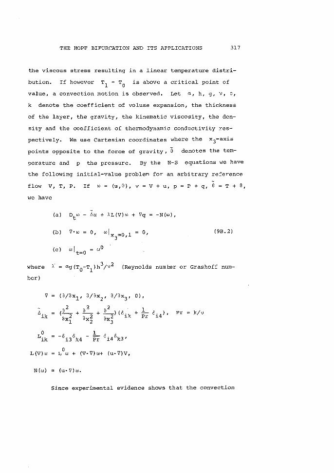
THE HOPF BIFURCATION AND ITS APPLICATIONS 317
the viscous stress resulting in a linear temperature distri-
bution. If however is above a critical point of
value, a convection motion is observed. Let a, h, g, v, P,
k denote the coefficient of volume expansion, the thickness
of the layer, the gravity, the kinematic viscosity, the den-
sity and the coefficient of thermodynamic conductivity res
pectively. We use Cartesian coordinates where the x 3-axis
points opposite to the force of gravity, 8 denotes the tem-
perature and p the pressure. By the N-S equations we have
the following initial-value problem for an arbitrary reference
flow V, T, P. If W = (u,8), v = V + u, P = P + q, 8 = T + 8,
we have
-(a) DtW - ~w + AL(V)w + Vq = -N(W),
(b) V'w 0, wl x =0,13
0, (9B.2)
(c) wi = wOt=O
where A = ag(To-Tl)h3/v2 (Reynolds numJ::er or Grashoff num
ber)
v (a/axl , a/ax2
, a/ax3
, 0) ,
a2 ?
a2
+,L~ik
L °i4) , Pr k/v(-2 +ax 2
+ -2) (oik PraXl 2 aX3
0 -0 ° _,L °i40k3'Lik i3 k4 Pr
L(V)w0
(V·V)w+ (u' V)V,L W +
N(w) (u· V)w.
Since experimental evidence shows that the convection

318 THE HOPF BIFURCATION AND ITS APPLICATIONS
takes place in a regular pattern of closed cells having the
form of rolls, we are going to consider the class of solutions
such that
w(Tx,t) w(x,t) , q{Tx,t) = q{x,t)
where T E Tl
, and Tl
is the group generated by the translations
x ....1
u{Tx,t)
q(Tx,t)
Tu{x,t)
q (x,t)
e(Tx,t) e (x,t)
where T2
is the group of rotations generated by
(c?s " -sin a 0Ta S1.n a cos a0 0
Note. It is possible to show that all differential
operators in the differential equation preserve invariance
under Tl and T2
• An interesting fact is that a necessary
condition for the existence of nontrivial solutions is
a = 21f/n, n E {1,2,3,4,6}, and that there are only 7 pos-
sible combinations of n,a,S, which give different cell pat-
terns (no cell structure, rolls, rec~angles, hexagons, squares,
triangles) •
Functional-Analytic Approach.
The analogy between (9B.l) and (9B.2) in the Taylor's and

THE HOPF BIFURCATION AND ITS APPLICATIONS 319
Benard's models suggests to the authors an abstract formula-
tion of the bifurcation and stability problem. In this part
I am going to sketch the idea that the authors follow to con
vert the differential equations (9B.l) and (9B.2) in a suitable
evolution equation in some Hilbert space.
We may consider D an open subset of R3 with bound
ary dD which is supposed to be a two dimensional C2-mani-
fold. Tl
denotes a group of translations and ~ its funda
mental region of periodicity which we may suppose is bounded.
AssumeD U T~.
'lET1
Now we consider the following sets (ct closure)
{wlw: ct(D) + Rn , infinitely often differentiable
in ct(D), w(Tx) = w(x), T E Tl
},
{wlw E CT,oo(D), supp weD},
Defining
0, w
f (DYv(x)·DYW(x))dxw
where
(v,w)'m
L (DYv,DYW),IY I:.m
Ivlm
and Y is a multiindex of length 3; one obtains the follow-
ing Hilbert spaces
aTHl,a
For the Taylor problem we have

320 THE HOPF BIFURCATION AND ITS APPLICATIONS
n 3, D
and for the Benard problem
n = 4, D = R2x (0,1), R the real numbers
n [0,21T/a) x [0,21T/13) x (0,1)
We may consider that the differential equations of theT
form (9B.l) or (9B.2) are written with operators in L2 .
From H. Weyl's lemma it is possible to consider L~aT
GT,
TJ E& where G contains the set of V such thatq
TLT
->-aT
q E Hl . We may use the orthogonal projection P:2
J
for removing the differential equation D w - ~w + AL(V)w +t
AVq = -AN(w) with the additional conditions of boundary and
and since we look for solutions on
Pu = u, and we may write the new equation inaTJ
If we con-periodicity, to a differential equation in
Tq E H
l, pVq == 0sider
aTJ , we have
as
dw + P~u + APL(V)at -APN(w) (9B.3)
owith initial condition wt=O = w .
The authors write (9B.3) in the form
dw + A(A)w + h(A)R(w)dt
0,o
w ,
-where A(A) = P~ + APL(V), R(W) = PN(w) and where heAl A
for Taylor's model and heAl 1 for Benard's model.
Also l they show using a result of Kato-Fujita, that it-
is possible to define fractional powers of A(A) by

THE HOPF BIFURCATION AND ITS APPLICATIONS 321
- -S 1 foo - S-lA(A) = f(Ff oexP(-A(A)t)t dt,
and that this operator is invertible.
13 > 0,
The ahove fact is useful in resolving some bifurcation
problems in the stationary case. If A = P~, M(V) = PL(V)
the stationary equation form (9B.3) is
(Sp) Aw + AM(V)w + h(A)R(w) °where V is any known stationary solution with V E Domain
of A.
If we consider the substitution = v
K(V)-1/4 3/4
A M(V)A-
we may write (Sp) in the form
v + AK(V) + h(A)T(v) = 0.
If one uses a theorem of Krasnoselskii, it is possible to
show the following theorem.
Theorem 4.1. Let be A. E R, A. f ° andJ J
an eigenvalue of K of odd multiplicity, then
(-A. )-1 beJ
i) in every neighborhood of
there exists (A,W), ° f W E D(A)
stationary equation (SP).
(A. ,0)J
such that
in
W solves the
ii) if (_A.)-l is a simple eigenvalue, then thereJ
exists a unique curve (A(a),w(a» such that weal f ° for
a f ° which solves (SP), moreover (A(O),W(O» = (A.,O).J
Now if we assume that V E C(IT)00
and dD is a C
manifold which is satisfied for the Taylor and B~nard Problem,

322 THE HOPF BIFURCATION AND ITS APPLICATIONS
and we consider solutions of (Sp) on the space Hm+2 n Hl,a'
m > 3/2, we may write the (SP) equation in the form
(SP) , Amw + \Mw + h(\)R(w) = °where is an operator whose domain is D(Am) = H
m+2n
HI, a C PRm, Am (w) = AW, wED (A) • If besides we consider
that in R(w) = PN(w), N(w) is an arbitrary polynomial opera-
tor including differentiation operators up to the order 2,
and Km MA~l we may obtain the following theorem.
Theorem 4.2. Let V E C(D), dD be a Coo-manifold;
and fulfill the boundary
plicity, (\ . ,0) is aJ
tions w are in cO)")
condition wlaD = 0.
let M such that there exists constants Cl
and C2 such
that IMWlm+l ~ cllwlm+2 and /MA:lwl m+l ~ c2lwlm. Then
for every eigenvalue (_\.)-1 of K, \. f 0, of odd multi-J m J
bifurcation point of (SP) '. The solu-
We may note that this theorem shows that we may obtain
a strong regularity for the branching solutions. Besides,
we note that in theorems 4.1 and 4.2 the existence of non-
trivial solutions of (SP) is reduced to the investigation
of the spectrum of K or Km•
Now, we are going to apply these theorems to the
Taylor's and Benard models.
Taylor Model. For this model we take K = A:l/4M(vO)A-3/4
the solution is given by
where ov is the Couette flow. In cylindrical
° °v (O,v~,O) where
coordinates
°v~ = ar + b/r
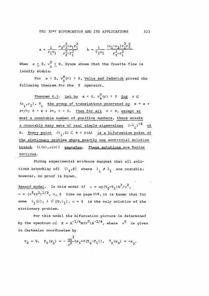
THE HOPF BIFURCATION AND ITS APPLICATIONS 323
a b
When a ~ 0, v~ > 0, Synge shows that the Couette flow is
locally stable.
For a < 0, v~(r) > 0, Velte and Judovich proved the
following theorem for the K operator.
Theorem 4.3. Let be °a < 0, v~(r) > ° for r E
(rl,r2 ), T
lthe group of translations generated by z + z +
2TI/a; ~ + ~ + 2TI, a > 0. Then for all a > 0, except at
most a countable number of positive numbers, there exists
a countably many sets of real simple eigenvalues (-A.) -1 of1.
K. Every point (Ai,O) E R x D(A) is a bifurcation point of
the stationary problem where exactly one nontrivial solution
branch (A(~),w(~» emanates. These solutions are Taylor
vortices.
Strong experimental evidence suggest that all solu-
tions branching off (Ai,O) where Ai f Al are unstable;
however, no proof is known.
Benard model. In this model if
a = (~2+S2)1/2, ~,. S like on page3l8, it is known that for
some Al (a), A E [O,A l ], w = ° is the only solution of the
stationary problem.
For this model the bifurcation picture is determined
by the spectrum of K = A-l/4M(VO)A-3/4, where v O is given
in Cartesian coordinates by
324 THE HOPF BIFURCATION AND ITS APPLICATIONS
In order to obtain simple eigenvalues, Judovich introduces
even solutions u(-x) = (-ul
(x) ,-u2
(x) ,u3 (x», 8(-x) = 8(x),
g(-x) = -q(x), and he shows in his articles, On the origin of
convection (Judovich [6]) and Free convection and bifurcation
(1967) the following theorem.
Theorem 4.6. i) The Benard problem possesses for ap-
prximately all a and B countably many simple positive
characteristic values A.• Furthermore (A. ,0) E R x D(A) is1 . 1
a bifurcation point.
ii) If n, a, B are chosen according to the note on
pg. 318, the branches emanating from (Ai,O) are doubly
periodic, rolls, hexagons, rectangles, and triangles.
iii) If Al denotes the smallest characteristic value,
then the nontrivial solution branches to the right of A~
and permits the parametrization W(A) = ±(A-Al)1/2F (A) where
F: R + D(A) is holomorphic in (A-Al
)1/2.
It is interesting to observe that since the character-
istic values are determined only by 0, we may consider dif-
ferentials a, B with the same value of 0, and to note that
we have solutions of every possible cell structure emanating
from each bifurcation point.
Stability.
About this topic I am going to give a short descrip-
tion of the principal results.
It is known that the basic solution loses stability
as in the past section. Under
the assumption that Ac simple, the nontrivial
THE HOPF BIFURCATION AND ITS APPLICATIONS 325
solution branch emanating from (AI,O) gains stability for
A > Al and is unstable for A < AI' This result can be de
rived using Leray-Schauder degree or by analytic perturba
tion methods.
Precisely if we take +V = Vo + w where is a
stationary solution of (SP) V is called stable if for
A(A) = A + AM(V), W = 0 is stable in sense with respect to
strict solutions in D(AS), 3/4 < S < 1. (Strict solution in
the sense of Kato-Fujita of the article), and V is called
unstable if it is not stable in ST. If we consider that
the nontrivial solution branch (A(a),V(a» in R x
lal < I (A(O),V(O» = (AlvO) can be written in the form
a(A)r E N
where F: R +D(A) is analytic in (A-AI)I/r and F(AI
) f 0
(valid conditions for Benard's and Taylor's models (Theorem
4.6 and Corollary 4.4), we have the following Theorem or
Lemma 5.6.
Lemma 5.6. Assume AC
= Al and Re ~ > a > 0 for all
nonvanishing ~ in the spectrum of G(A(AI,VO»' Let Al
be a simple characteristic value of K(V O)' 0 a simple eigen
value of A(AI,vO)'
Then, if A is restricted to a suitable neighborhood
of Al
i) Vo is stable for A < Al and unstable for
A > AI
ii) veAl is stable for A > Al and unstable for

326 THE HOPF BIFURCATION AND ITS APPLICATIONS
For the B~nard's model, the assumptions of Lemma 5.6
are satisfied for fixed n, a, S; A1 is a simple character
istic value of K(V O) by Theorem 4.6 and AC
= A1 follows
from Lemma 4.50f the article.
For the Taylor's model only the simplicity of A1 as
a characteristic value of K(VO) is known. The simplicity
of ~ = 0 in 0(AA 1 ,VO
) is an open problem.
However, we may give the following theorem.
Theorem 5.7. i) For the Benard's problem, every solu
tion with a given cell pattern (fixed n, a, S) exists in
some right neighborhood of A1 and is asymptotically stable
in D(AS), S E (3/4,1). The basic solution Vo is asymptoti
cally stable for A < A1
and unstable for A > A1
•
ii) For the Taylor's problem, let the assumptions of
Lemma 5.6 on the spectrum of A(A;VO) be valid. Then for
every period (0 fixed) V(A) is asymptotically stable if it
exists for A > A1
, and is unstable if it exists for A < A1
•
Finally, we remark that these results can also be ob-
tained using the invariant manifold approach. (See, for
example, Exercise 4.3). That this is possible was noted a1-
ready by Rue11e-Takens [1] in their elegant and simple
proof of Velte's theorem. We also note that Prodi's basic
results relating the spectral and stability properties of the
Navier-Stokes equations are contained in the smoothness pro-
perties of the flow from Section 9 and the results of Sec-
tion 2A.