Section 8.3

Suppose X1 , X2 , ..., Xn are a random sample from a distribution defined by the p.d.f.

f(x) for a < x < b and corresponding distribution function F(x),

The random variables which order the sample from smallest to largest Y1 < Y2 < ...< Yn are called the order statistics.

Suppose n = 2.

The space of (X1 , X2) is

The space of (Y1 , Y2) is

{(x1 , x2) | a < x1 < b , a < x2 < b}

{(y1 , y2) | a < y1 < y2 < b }

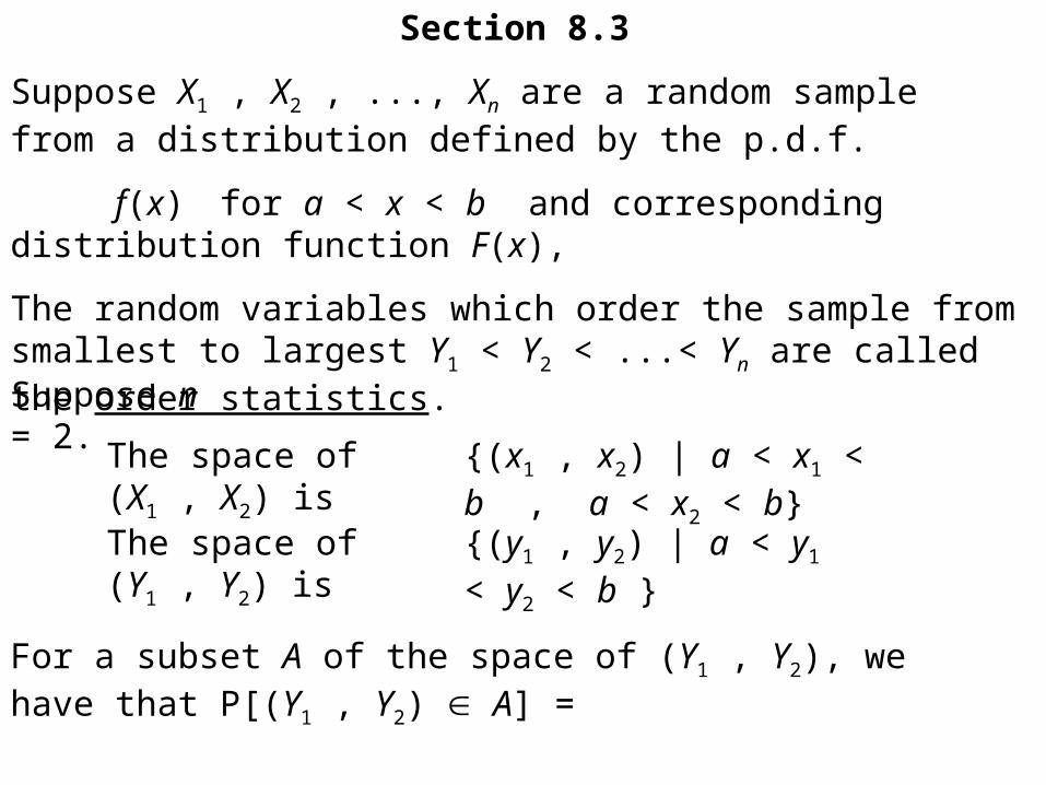
For a subset A of the space of (Y1 , Y2), we have that P[(Y1 , Y2) A] =

For a subset A of the space of (Y1 , Y2), we have that P[(Y1 , Y2) A] =

P[{(X1 , X2) A}{(X2 , X1) A}] =P[(X1 , X2) A] + P[(X2 , X1) A] =

2 P[(X1 , X2) A] =

A

2 dx1 dx2 =f(x1) f(x2)

A

2 f(y1) f(y2) dy1 dy2

Therefore, the joint p.d.f. of (Y1 , Y2) must be

g(y1 , y2) = 2 f(y1) f(y2) if a < y1 < y2 < b

To find the p.d.f. for Y1 , we first find the distribution function

G1(y) = P(Y1 ≤ y) = P[min(X1 , X2) ≤ y] = 1 – P[min(X1 , X2) y] =

1 – P(X1 y X2 y) =

1 – P(X1 y) P(X2 y) =1 – [1 – P(X1 ≤ y)] [1 – P(X2 ≤ y)] = 1 – [1 – F(y)] [1 – F(y)] =

1 – [1 – F(y)]2

The p.d.f. for Y1 is g1(y) =

d—G1(y) =dy

– 2[1 – F(y)][– f(y)] = 2[1 – F(y)]f(y) if a < y < b

To find the p.d.f. for Y2 , we first find the distribution function

G2(y) = P(Y2 ≤ y) = P[max(X1 , X2) ≤ y] = P(X1 ≤ y X2 ≤ y) =

P(X1 ≤ y) P(X2 ≤ y) = F(y)F(y) = [F(y)]2

The p.d.f. for Y2 is g2(y) = d—G2(y) =dy

2F(y)f(y) if a < y < b

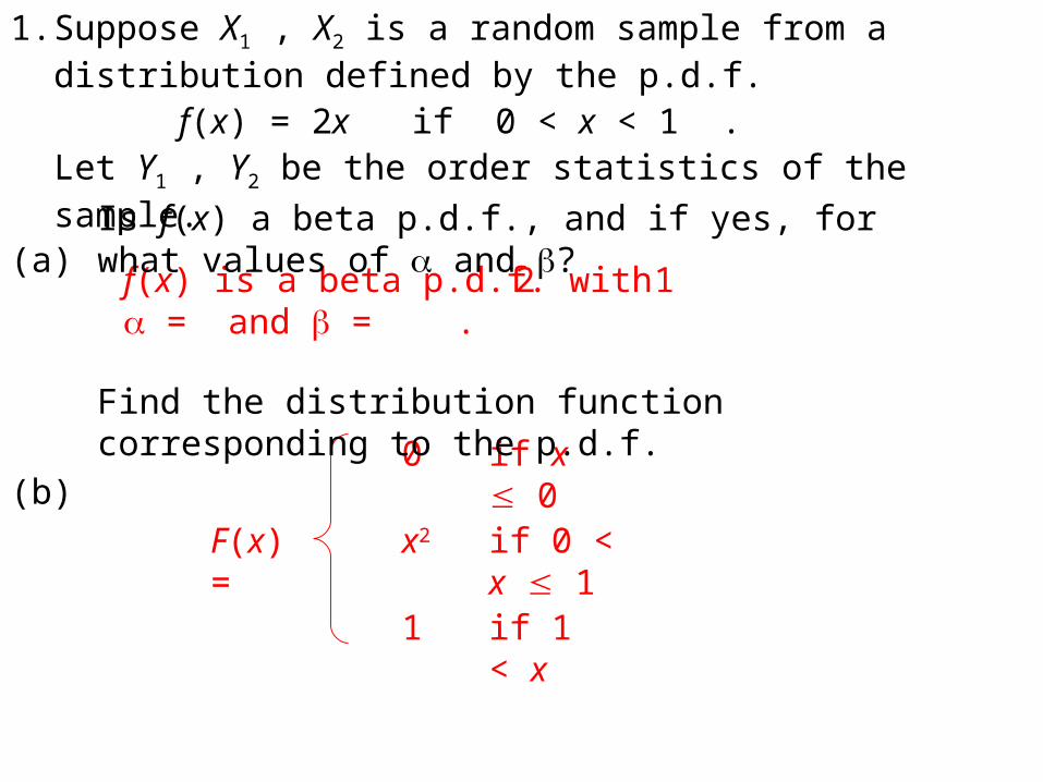
F(x) =

if x 0

0

if 0 < x 1

x2

if 1 < x1

f(x) is a beta p.d.f. with = and = .2 1

1.

(a)

(b)

Suppose X1 , X2 is a random sample from a distribution defined by the p.d.f.

f(x) = 2x if 0 < x < 1 .Let Y1 , Y2 be the order statistics of the sample.

Is f(x) a beta p.d.f., and if yes, for what values of and ?

Find the distribution function corresponding to the p.d.f.

(c)

(d)

(e)

(f)

Find the joint p.d.f. of the order statistics (Y1 , Y2).

The joint p.d.f. of Y1 , Y2 is

g(y1 , y2) = 2(2y1)(2y2) = 8y1y2 if 0 < y1 < y2 < 1

Find the p.d.f. of Y1 .

Find the p.d.f. of Y2 .

Is either the p.d.f. of Y1 or the p.d.f. of Y2 a beta p.d.f., and if yes, for what values of and ?

The p.d.f. of Y1 is g1(y) =

2[1 – y2](2y) = 4y(1 – y2) if 0 < y < 1

The p.d.f. of Y2 is g2(y) =

2[y2](2y) = 4y3 if 0 < y < 1

The p.d.f. of Y1 is not a beta p.d.f.

The p.d.f. of Y2 is a beta p.d.f. with = and = .4 1

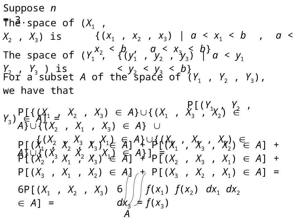
Suppose n = 3.

The space of (X1 , X2 , X3) is

The space of (Y1 , Y2 , Y3 ) is

{(x1 , x2 , x3) | a < x1 < b , a < x2 < b , a < x3 < b}

{(y1 , y2 , y3) | a < y1 < y2 < y3 < b}

For a subset A of the space of (Y1 , Y2 , Y3), we have that

P[(Y1 , Y2 , Y3) A] =

P[{(X1 , X2 , X3) A}{(X1 , X3 , X2) A}{(X2 , X1 , X3) A} {(X2 , X3 , X1) A}{(X3 , X1 , X2) A}{(X3 , X2 , X1) A}] =

P[(X1 , X2 , X3) A] + P[(X1 , X3 , X2) A] + P[(X2 , X1 , X3) A] + P[(X2 , X3 , X1) A] + P[(X3 , X1 , X2) A] + P[(X3 , X2 , X1) A] =

6P[(X1 , X2 , X3) A] =

A

6 dx1 dx2 dx3 =f(x1) f(x2) f(x3)

6P[(X1 , X2 , X3) A] =

A

6 dx1 dx2 dx3 =f(x1) f(x2) f(x3)

A

6 f(y1) f(y2) f(y3) dy1 dy2 dy3

g(y1 , y2 , y3) = 6 f(y1) f(y2) f(y3) if a < y1 < y2 < y3 < b

Therefore, the joint p.d.f. of (Y1 , Y2 , Y3) must be

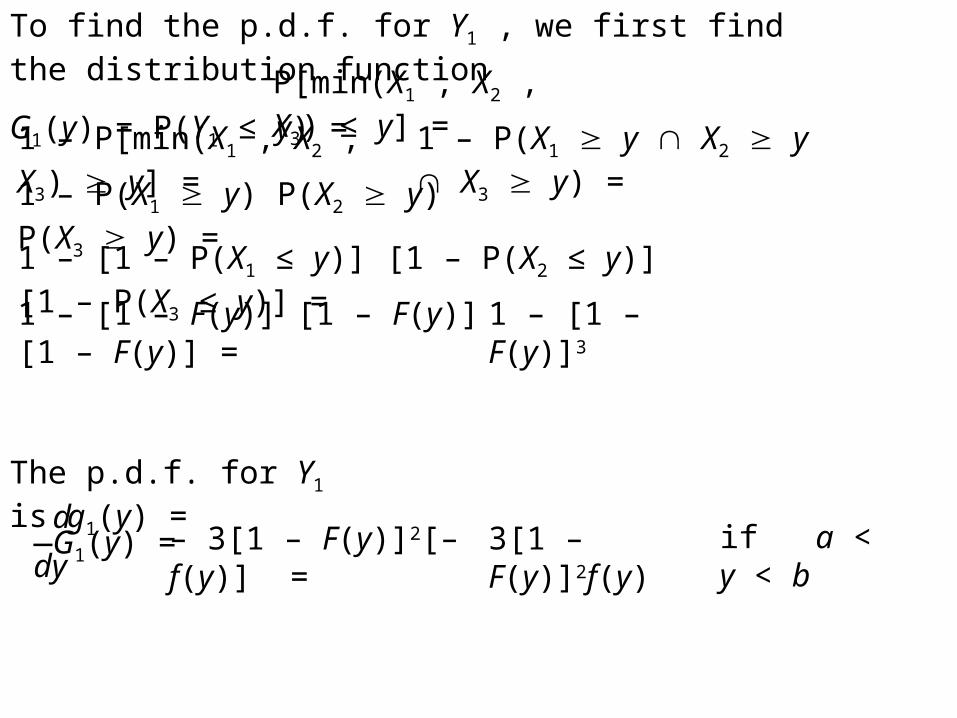
To find the p.d.f. for Y1 , we first find the distribution function

G1(y) = P(Y1 ≤ y) = P[min(X1 , X2 , X3) ≤ y] =

1 – P[min(X1 , X2 , X3) y] =

1 – P(X1 y X2 y X3 y) =1 – P(X1 y) P(X2 y) P(X3 y)

=1 – [1 – P(X1 ≤ y)] [1 – P(X2 ≤ y)] [1 – P(X3 ≤ y)] =

1 – [1 – F(y)] [1 – F(y)] [1 – F(y)] = 1 – [1 – F(y)]3

The p.d.f. for Y1 is g1(y) =

d—G1(y) =dy

– 3[1 – F(y)]2[– f(y)] = 3[1 – F(y)]2f(y) if a < y < b

To find the p.d.f. for Y2 , we first find the distribution function

G2(y) = P(Y2 ≤ y) = P[at least two of X1 , X2 , X3 are y] =

3

2[ ]2 [1 – ]1 + [ ]3 [1 – ]0 =

3

3F(y) F(y) F(y) F(y)

3[F(y)]2 [1 – F(y)] + [F(y)]3

The p.d.f. for Y2 is g2(y) =

d—G2(y) =dy

6[F(y)]f(y)[1 – F(y)] + 3[F(y)]2 [– f(y)] + 3[F(y)]2 f(y) =

6[F(y)] [1 – F(y)] f(y) if a < y < b

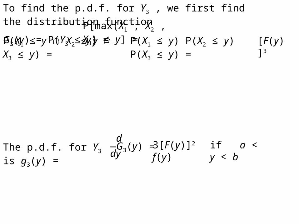
To find the p.d.f. for Y3 , we first find the distribution function

G3(y) = P(Y3 ≤ y) = P[max(X1 , X2 , X3) ≤ y] =

P(X1 ≤ y X2 ≤ y X3 ≤ y) = P(X1 ≤ y) P(X2 ≤ y) P(X3 ≤ y) = [F(y)]3

The p.d.f. for Y3 is g3(y) = d—G3(y) =dy

3[F(y)]2 f(y) if a < y < b

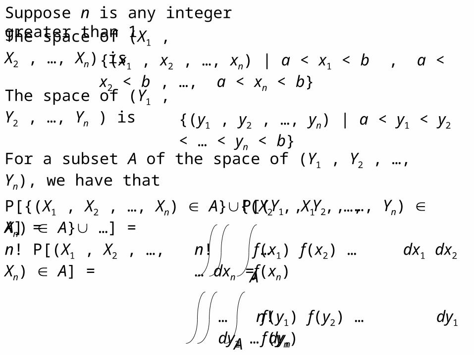
Suppose n is any integer greater than 1.

The space of (X1 , X2 , …, Xn) is

The space of (Y1 , Y2 , …, Yn ) is

{(x1 , x2 , …, xn) | a < x1 < b , a < x2 < b , …, a < xn < b}

{(y1 , y2 , …, yn) | a < y1 < y2 < … < yn < b}

For a subset A of the space of (Y1 , Y2 , …, Yn), we have that

P[(Y1 , Y2 , …, Yn) A] =

P[{(X1 , X2 , …, Xn) A}{(X2 , X1 , …, Xn) A} …] =

n! P[(X1 , X2 , …, Xn) A] =

A

n! … dx1 dx2 … dxn =f(x1) f(x2) … f(xn)

A

… n! dy1 dy2 … dynf(y1) f(y2) … f(yn)

Therefore, the joint p.d.f. of (Y1 , Y2 , …, Yn) must be

g(y1 , y2 , …, yn) = n! f(y1) f(y2) … f(yn) if a < y1 < y2 < … < yn < b

Suppose r is any integer from 1 to n.

To find the p.d.f. for Yr , we first find the distribution function

Gr(y) = P(Yr y) = P [at least r of X1 , X2 , …, Xn are y] =

n

[ ]k [1 – ]n–k

k = r

n

k F(y) F(y)

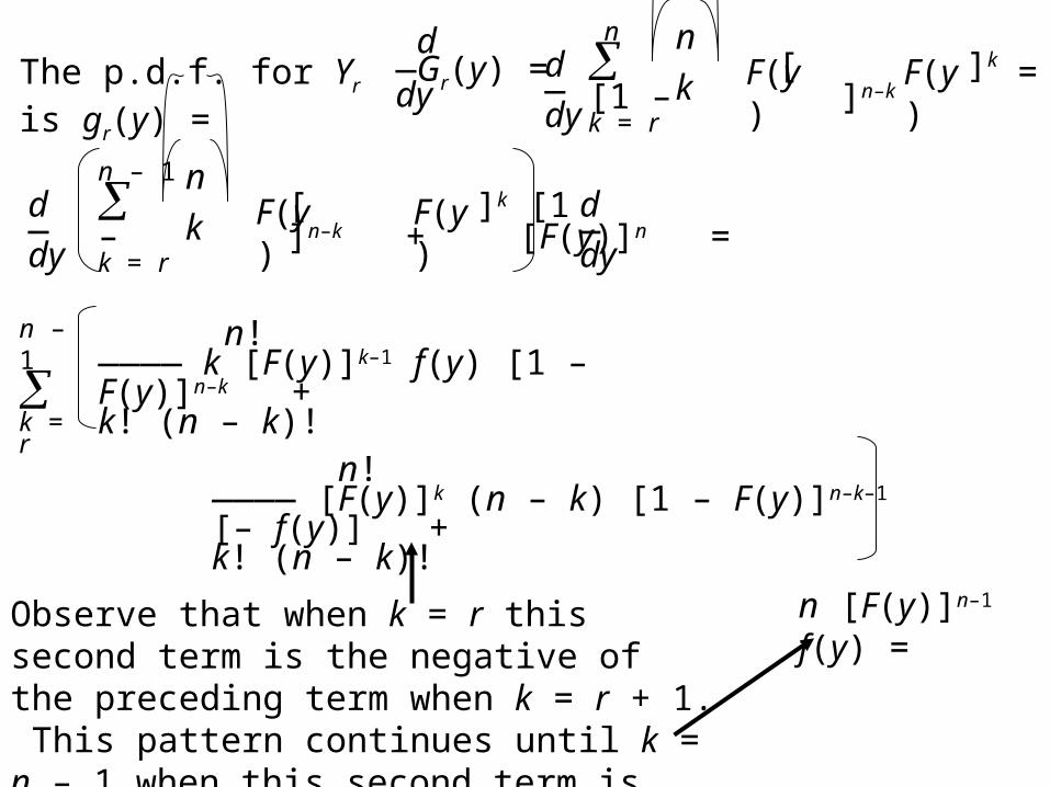
The p.d.f. for Yr is gr(y) = d—Gr(y) =dy

n

[ ]k [1 – ]n–k

k = r

n

k F(y) F(y) d—dy

n – 1

[ ]k [1 – ]n–k + [F(y)]n =k = r

n

k F(y) F(y) d—dy

d—dy

n – 1

k = r

n!———— k [F(y)]k–1 f(y) [1 – F(y)]n–k +k! (n – k)!

n!———— [F(y)]k (n – k) [1 – F(y)]n–k–1 [– f(y)] +k! (n – k)!

n [F(y)]n–1 f(y) =Observe that when k = r this second term is the negative of the preceding term when k = r + 1. This pattern continues until k = n – 1 when this second term is the negative of the isolated term.

=

if a < y < b

Consequently, the p.d.f. for Yr is gr(y) =

n!—————— [F(y)]r–1 [1 – F(y)]n–r f(y)(r – 1)! (n – r)!

Now, go to Exercise #2:

Suppose the random sample X1 , X2 , X3 , X4 , X5 is from a distribution defined by the p.d.f.

f(x) = 2x if 0 < x < 1 .Let Y1 , Y2 , Y3 , Y4 , Y5 be the order statistics of the sample.

Find the joint p.d.f. of the order statistics (Y1 , Y2 , Y3 , Y4 , Y5).

2.

(a)

(b)

The joint p.d.f. of Y1 , Y2 , Y3 , Y4 , Y5 is

g(y1 , y2 , y3 , y4 , y5) = 3840 y1 y2 y3 y4 y5

if 0 < y1 < y2 < y3 < y4 < y5 < 1

Find the p.d.f. of Y1 .

The p.d.f. of Y1 is g1(y) =

5!—————— [y2]1–1 [1 – y2]5–1 (2y) =(1 – 1)! (5 – 1)!

10y(1 – y2)4 if 0 < y < 1

(c)

(d)

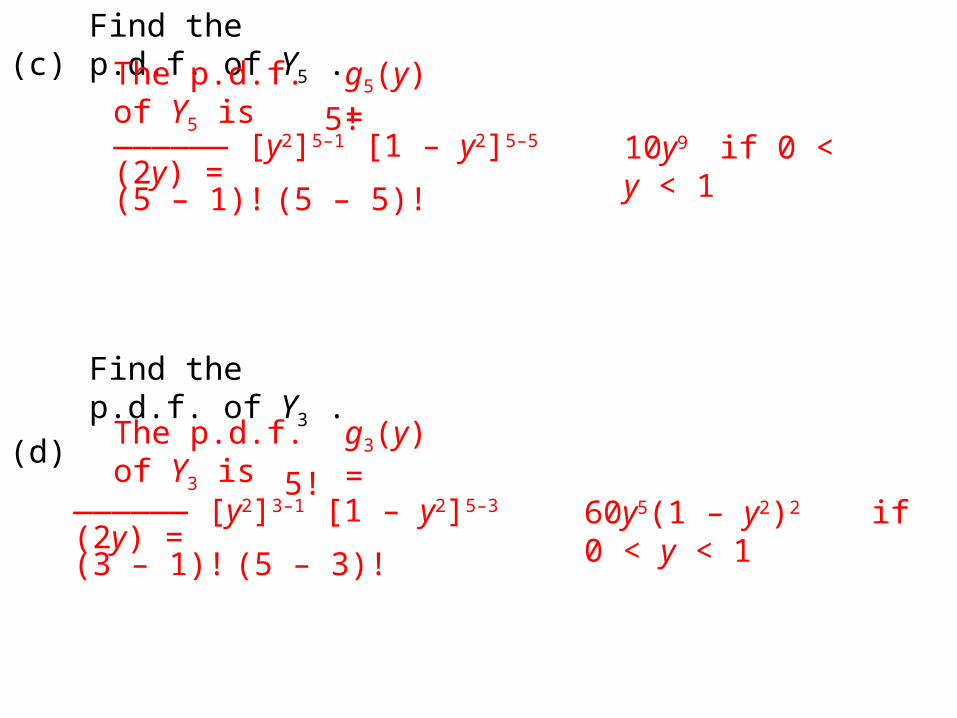
Find the p.d.f. of Y5 .

Find the p.d.f. of Y3 .

The p.d.f. of Y5 is g5(y) =

5!—————— [y2]5–1 [1 – y2]5–5 (2y) =(5 – 1)! (5 – 5)!

10y9 if 0 < y < 1

The p.d.f. of Y3 is g3(y) =

5!—————— [y2]3–1 [1 – y2]5–3 (2y) =(3 – 1)! (5 – 3)!

60y5(1 – y2)2 if 0 < y < 1

2.-continued

(e) Find P(Y1 1/2).

P(Y1 1/2) =

0

1/2

10y(1 – y2)4 dy =

0

1/2

– 5 – 2y(1 – y2)4 dy =

(1 – y2)5

– 5 ———— = 5

y = 0

1/2

31 – —

4

5

Note that an alternative approach is

P(Y1 1/2) = P[min(X1 , X2 , X3 , X4 , X5) 1/2] =

781= —— 1024

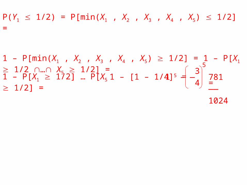
P(Y1 1/2) = P[min(X1 , X2 , X3 , X4 , X5) 1/2] =

1 – P[min(X1 , X2 , X3 , X4 , X5) 1/2] = 1 – P[X1 1/2 … X5 1/2] =

1 – P[X1 1/2] … P[X5 1/2] =

1 – [1 – 1/4]5 = 3

1 – — 4

5 781= —— 1024

Find P(Y5 1/2).

2.-continued

(f)

P(Y5 1/2) =

0

1/2

10y9 dy = y10 =

y = 0

1/2 1— 2

10

Note that an alternative approach is

P(Y5 1/2) = P[max(X1 , X2 , X3 , X4 , X5) 1/2] =P[X1 1/2 … X5 1/2] =

P[X1 1/2] … P[X5 1/2] =

([1/2]2)5 = 1— 2

10 1= —— 1024

2.-continued

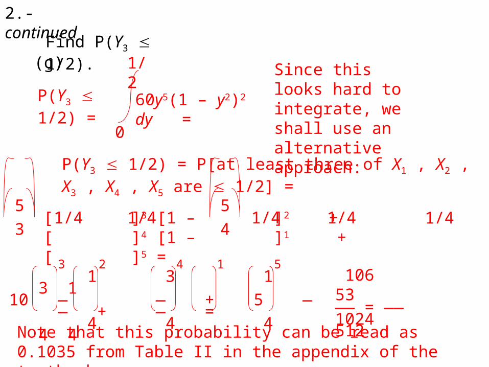
(g) Find P(Y3 1/2).

P(Y3 1/2) =

0

1/2

60y5(1 – y2)2 dy =

Since this looks hard to integrate, we shall use an alternative approach:

P(Y3 1/2) = P[at least three of X1 , X2 , X3 , X4 , X5 are 1/2] =

5

3[ ]3 [1 – ]2 + [ ]4 [1 – ]1 + [ ]5 =

5

41/4 1/4 1/4 1/4 1/4

1 3 1 3 110 — — + 5 — — + — = 4 4 4 4 4

3 2 4 1 5 106 53—— = ——1024 512

Note that this probability can be read as 0.1035 from Table II in the appendix of the textbook.

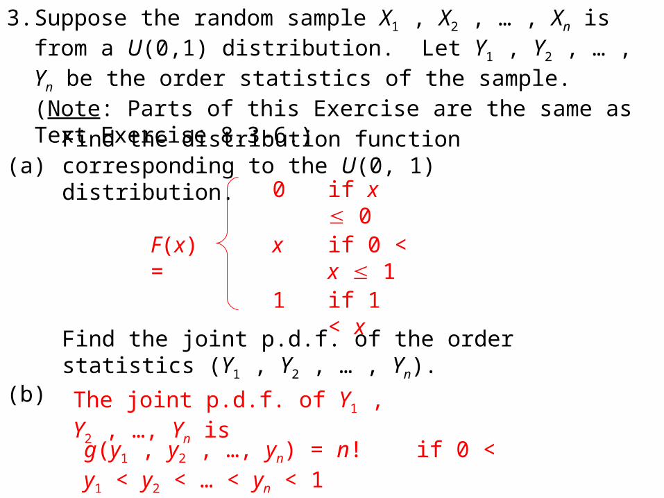
Suppose the random sample X1 , X2 , … , Xn is from a U(0,1) distribution. Let Y1 , Y2 , … , Yn be the order statistics of the sample. (Note: Parts of this Exercise are the same as Text Exercise 8.3-6.)

Find the distribution function corresponding to the U(0, 1) distribution.

3.

(a)

(b)

F(x) =

if x 0

0

if 0 < x 1

x

if 1 < x1

Find the joint p.d.f. of the order statistics (Y1 , Y2 , … , Yn).

The joint p.d.f. of Y1 , Y2 , …, Yn is

g(y1 , y2 , …, yn) = n! if 0 < y1 < y2 < … < yn < 1

(c) Find the p.d.f. of Yr where r is any integer from 1 to n.

The p.d.f. of Yr is gr(y) = n!—————— yr–1 (1 – y)n–r if 0 < y < 1(r – 1)! (n – r)!

Realizing that (n + 1) = n! , (r) = (r – 1)! , and (n – r + 1) = (n – r)!, we find that Yr has a distributionbeta rwith = and = n – r + 1 .

This is essentially what Text Exercise 8.3-6(c) says to show.

3.-continued

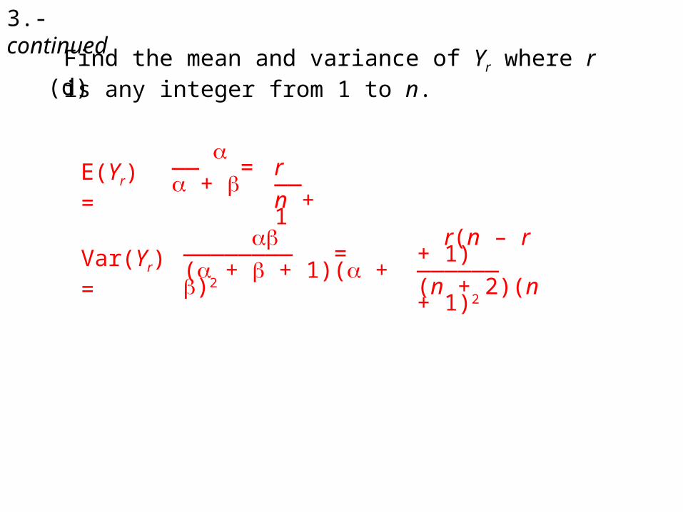
(d) Find the mean and variance of Yr where r is any integer from 1 to n.

E(Yr) = —— = +

r——n + 1

Var(Yr) =

———————— =( + + 1)( + )2

r(n – r + 1)——————(n + 2)(n + 1)2

E(Yr+1 – Yr) =r + 1—— –n + 1

r—— =n + 1

1——n + 1

(e) Find E(Yr+1 – Yr) where r is any integer from 1 to n – 1.

4.

(a)

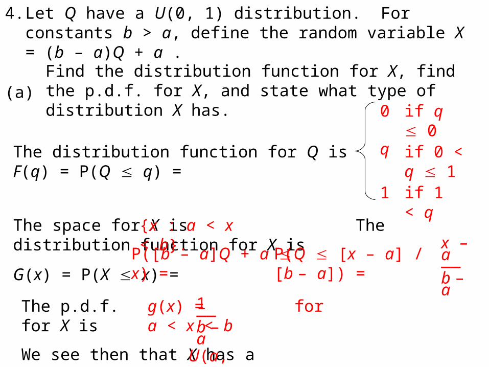
Let Q have a U(0, 1) distribution. For constants b > a, define the random variable X = (b – a)Q + a .

Find the distribution function for X, find the p.d.f. for X, and state what type of distribution X has.

The distribution function for Q is F(q) = P(Q q) =

if q 00

if 0 < q 1if 1 < q1

The space for X is The distribution function for X is

G(x) = P(X x) =

{x : a < x < b}.

P([b – a]Q + a x) =P(Q [x – a] / [b – a]) =

We see then that X has a distribution.U(a, b)

The p.d.f. for X is g(x) = for a < x < b

q

x – a——b – a

1——b – a

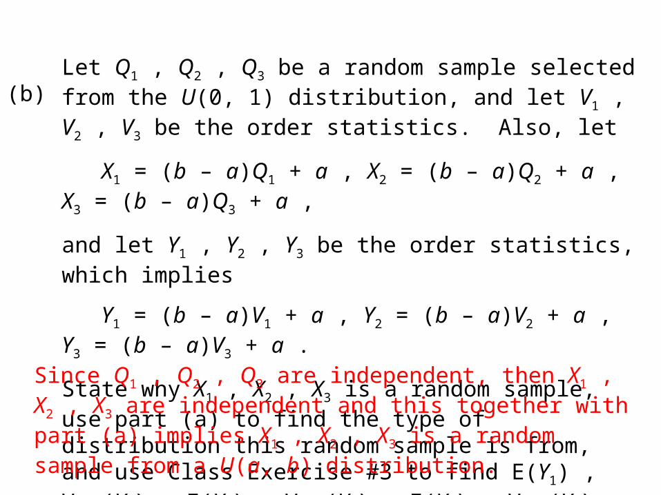
(b) Let Q1 , Q2 , Q3 be a random sample selected from the U(0, 1) distribution, and let V1 , V2 , V3 be the order statistics. Also, let

X1 = (b – a)Q1 + a , X2 = (b – a)Q2 + a , X3 = (b – a)Q3 + a ,

and let Y1 , Y2 , Y3 be the order statistics, which implies

Y1 = (b – a)V1 + a , Y2 = (b – a)V2 + a , Y3 = (b – a)V3 + a .

State why X1 , X2 , X3 is a random sample, use part (a) to find the type of distribution this random sample is from, and use Class Exercise #3 to find E(Y1) , Var(Y1) , E(Y2) , Var(Y2) , E(Y3) , Var(Y3) , and E(Y1Y3) .Since Q1 , Q2 , Q3 are independent, then X1 , X2 , X3 are independent

and this together with part (a) implies X1 , X2 , X3 is a random sample from a U(a, b) distribution.

4.-continued

E(Y1) =

Var(Y1) =

E(Y2) =

E([b – a]V1 + a) = [b – a]E(V1) + a = r

[b – a] —— + a =n + 1

b + 3a——— 4

1[b – a] —— + a =

3 + 1

Var([b – a]V1 + a) = (b – a)2Var(V1) =

r(n – r + 1)(b – a)2 —————— =

(n + 2)(n + 1)2

1(3 – 1 + 1)(b – a)2 —————— =

(3 + 2)(3 + 1)2

3(b – a)2

———– 80

E([b – a]V2 + a) = [b – a]E(V2) + a = r

[b – a] —— + a =n + 1

b + a—— 2

2[b – a] —— + a =

3 + 1

Var(Y2) =

E(Y3) =

Var(Y3) =

Var([b – a]V2 + a) = (b – a)2Var(V2) =

r(n – r + 1)(b – a)2 —————— =

(n + 2)(n + 1)2

2(3 – 2 + 1)(b – a)2 —————— =

(3 + 2)(3 + 1)2

(b – a)2

———– 20

E([b – a]V3 + a) = [b – a]E(V3) + a = r

[b – a] —— + a =n + 1

3b + a——— 4

3[b – a] —— + a =

3 + 1

Var([b – a]V3 + a) = (b – a)2Var(V3) =

r(n – r + 1)(b – a)2 —————— =

(n + 2)(n + 1)2

3(3 – 3 + 1)(b – a)2 —————— =

(3 + 2)(3 + 1)2

3(b – a)2

———– 80

4.-continued

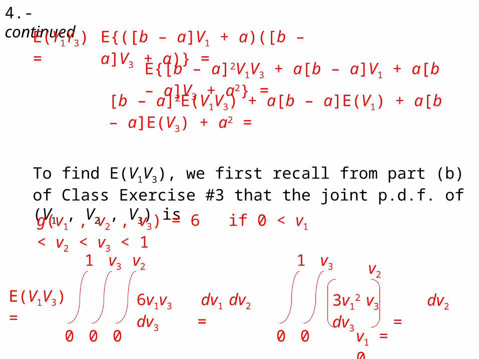
E(Y1Y3) = E{([b – a]V1 + a)([b – a]V3 + a)} =

E{[b – a]2V1V3 + a[b – a]V1 + a[b – a]V3 + a2} =

[b – a]2E(V1V3) + a[b – a]E(V1) + a[b – a]E(V3) + a2 =

To find E(V1V3), we first recall from part (b) of Class Exercise #3 that the joint p.d.f. of (V1 , V2 , V3) is

g(v1 , v2 , v3) = 6 if 0 < v1 < v2 < v3 < 1

E(V1V3) = 6v1v3 dv1 dv2 dv3 =

0

v2

0

v3

0

1

0

v3

0

1

3v12 v3 dv2 dv3 =

v1 = 0

v2

0

v3

0

1

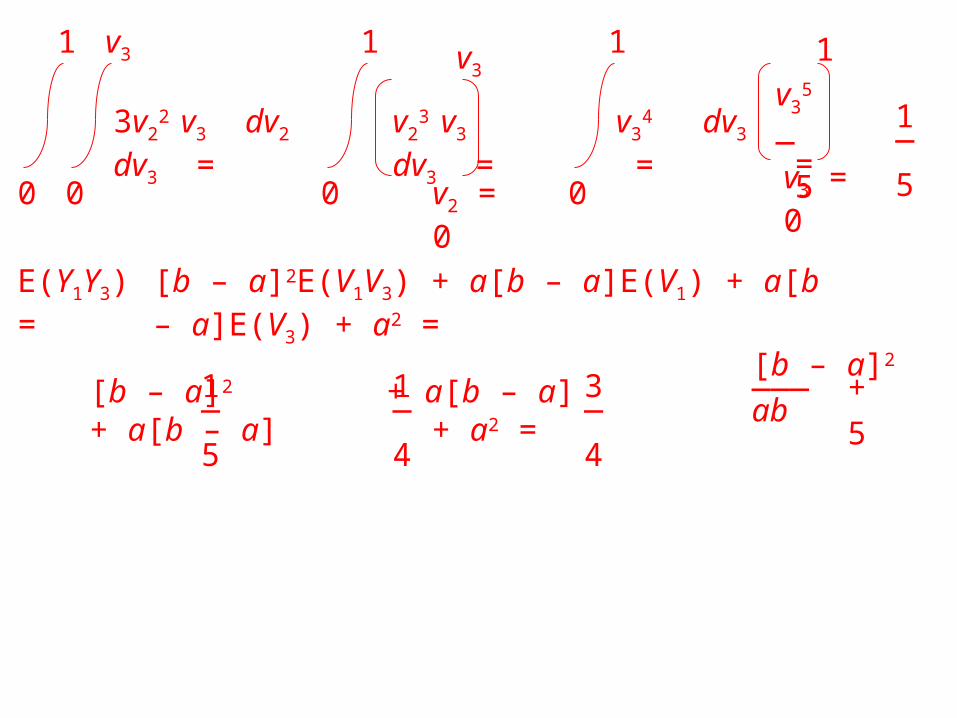
3v22 v3 dv2 dv3 =

0

1

v23 v3 dv3 =

v2 = 0

v3

0

1

v34 dv3 =

v35

— = 5v3 = 0

1 1— 5

E(Y1Y3) = [b – a]2E(V1V3) + a[b – a]E(V1) + a[b – a]E(V3) + a2 =

[b – a]2 + a[b – a] + a[b – a] + a2 = 1— 5

1— 4

3— 4

[b – a]2

——— + ab 5

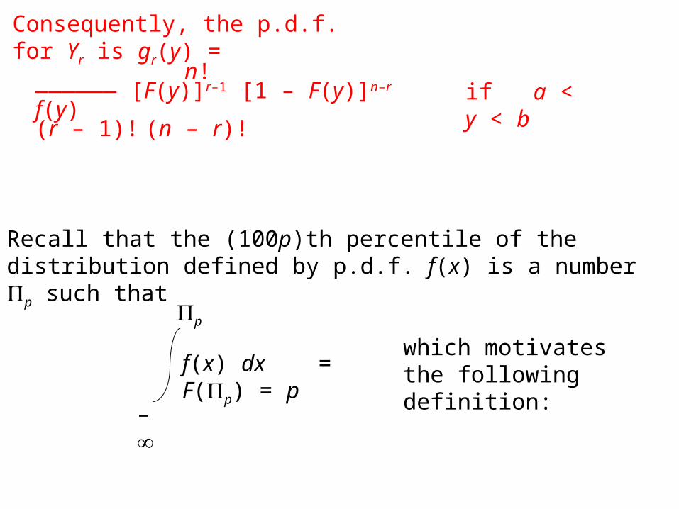
if a < y < b

Consequently, the p.d.f. for Yr is gr(y) =

n!—————— [F(y)]r–1 [1 – F(y)]n–r f(y)(r – 1)! (n – r)!

Recall that the (100p)th percentile of the distribution defined by p.d.f. f(x) is a number p such that

–

p

f(x) dx = F(p) = pwhich motivates the following definition:

The (100p)th percentile of the sample X1 , X2 , …, Xn is defined to be

Yr where r = (n+1)p

a weighted average of Yr and Yr+1 where r = (n+1)p

Note: This definition is extended to an observed sample of values x1 , x2 , …, xn where the ordered values in the sample are represented by y1 , y2 , …, yn .

if (n+1)p is not an integer

if (n+1)p is an integer

The detailed definition of sample order statistics was given in Section 3.2.

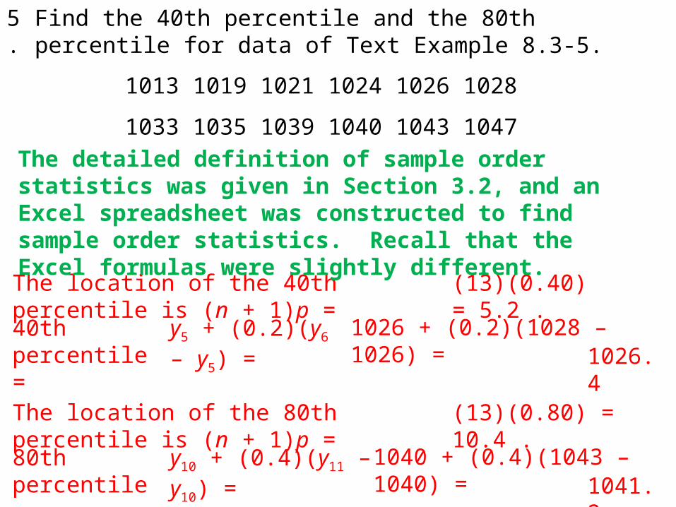
1013 1019 1021 1024 1026 1028

1033 1035 1039 1040 1043 1047

The location of the 40th percentile is (n + 1)p = (13)(0.40) = 5.2 .

40th percentile = y5 + (0.2)(y6 – y5) = 1026 + (0.2)(1028 – 1026) =1026.4

The location of the 80th percentile is (n + 1)p = (13)(0.80) = 10.4 .

80th percentile = y10 + (0.4)(y11 – y10) = 1040 + (0.4)(1043 – 1040) =1041.2

Find the 40th percentile and the 80th percentile for data of Text Example 8.3-5.

5.

The detailed definition of sample order statistics was given in Section 3.2, and an Excel spreadsheet was constructed to find sample order statistics. Recall that the Excel formulas were slightly different.