40  

SECTION 5 Magnetostatics

This section (based on Chapter 5 of Griffiths) deals mainly with magnetic effects produced by electric currents in the absence of a magnetic material. The topics are:

• The Lorentz Force Law • The Biot-Savart Law • The divergence and curl of B • Magnetic vector potential

The Lorentz Force Law Magnetic fields In electrostatics, we considered the force acting on a test charge due to some collection of charges, all of which were at rest. Now we want to look at forces on charges in motion.

• The force on a moving charge is not in the direction of the field, but perpendicular to it.

• Instead of stationary charges (as in electrostatics), magnetostatics looks at currents that do not change with time (steady flow of charge).

Lorentz force law The force due to a magnetic field B, acting on a charge Q moving at a velocity v, is:

Like the electric force E, this is derived from experiment and it provides us with the definition of B. In general, therefore, the total force on a charged particle is: Notes:

• Particles moving parallel to the magnetic field do not experience a magnetic force. • The magnetic force cannot do work, since it is always perpendicular to the motion of the particle. It

cannot change the speed of a particle, only its direction. Cyclotron motion A particularly interesting situation occurs when velocity v is perpendicular to B. The particle in this case travels in a circle of radius R:

I

q I2

I F

I

Fmag =Q(v!B)

F = Q[E+ (v!B)]

F = qvB =ma = mv2

R

If we hold a charge (at rest) next to a wire carrying current I, there is no force on the charge (assuming the wire to be overall electrically neutral).

If we place another current carrying wire alongside the first, it does experience a force. This is found to be attractive if the currents are in the same direction, and repulsive otherwise.

• The magnetic field circles a wire, in the direction given by the right hand rule (right thumb along wire, fingers show direction of magnetic field)

 

  41  

Currents Current: it is defined as charge per unit time (crossing a specified area). By convention, the current is taken in the direction of flow of positive charges (which is opposite the motion of negative charges). Units: Amperes = Coulombs / second 1 A = 1 C/s

A line charge λ travelling down a thin wire produces a current of magnitude: or vectorially For a thin wire the direction is usually obvious, but we sometimes we need to define current as a vector for use with surface and volume currents.

The force on a wire due to an external magnetic field B is:

Since the current and the line element of the wire are in the same direction, we can also write the last result as

Finally, if the current is constant along the wire,

Surface current

The surface current density is defined as:

Alternatively, if the charge per unit area of the mobile charges is σ, and the charges move with velocity v: The magnetic force is:

Volume currents If we have charge flowing through a 3-dimensional region, we can define a volume current. We look at a small tube of cross sectional area da! along the direction of the flow of charge. The volume current density is:

Again, if we have a mobile volume charge density of ρ, the current density is:

The magnetic force on a volume current is:

B

v

F

I = !v I = !v

Fmag = (v!B)" dq = (v!B)" !dl = (I!B)" dl

Fmag = I (dl!B)"

Fmag = I (dl!B)"

dl!

K

K =dIdl!

K =!v

Fmag = (v!B)" !da = (K!B)" da

J = dIda!

J = !v

Fmag = (v!B)" !d" = (J!B)" d"

       The cyclotron is a convenient way to measure the momentum (and hence kinetic energy) of a charged particle.  

If the current is flowing across a sheet, we can introduce a surface current. Consider a skinny ribbon (or stripe) of the surface, parallel to the charge flow, with width and carrying current dI.  

  42  

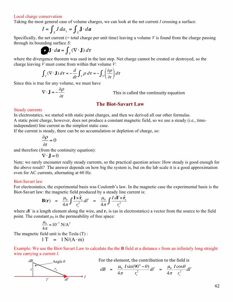
Local charge conservation Taking the most general case of volume charges, we can look at the net current I crossing a surface:

Specifically, the net current (= total charge per unit time) leaving a volume V is found from the charge passing through its bounding surface S:

where the divergence theorem was used in the last step. Net charge cannot be created or destroyed, so the charge leaving V must come from within that volume V:

Since this is true for any volume, we must have

The Biot-Savart Law Steady currents In electrostatics, we started with static point charges, and then we derived all our other formulas. A static point charge, however, does not produce a constant magnetic field, so we use a steady (i.e., time-independent) line current as the simplest static case. If the current is steady, there can be no accumulation or depletion of charge, so:

and therefore (from the continuity equation):

Note: we rarely encounter really steady currents, so the practical question arises: How steady is good enough for the above result? The answer depends on how big the system is, but on the lab scale it is a good approximation even for AC currents, alternating at 60 Hz. Biot-Savart law For electrostatics, the experimental basis was Coulomb’s law. In the magnetic case the experimental basis is the Biot-Savart law: the magnetic field produced by a steady line current is:

where dl’ is a length element along the wire, and re is (as in electrostatics) a vector from the source to the field point. The constant µ0 is the permeability of free space:

The magnetic field unit is the Tesla (T) :

Example: We use the Biot-Savart Law to calculate the the B field at a distance s from an infinitely long straight wire carrying a current I.

I = J da!S" = J #daS"

J !daS!" = (#! J)

V" d!

(!" J)V# d! = $ d

dt"

V# d! = $ %"%t

&

'(

)

*+

V# d!

!" J = #$!$t

!!!t

= 0

!" J = 0

B(r) =µ04!

I! r̂ere2" d #l =

µ04!

I d #l ! r̂ere2"

µ04!

=10!7 N/A2

1T = 1N/(A !m)

I

s re

l’ dl’

Angle ! dB For  the  element,  the  contribution  to  the  field  is  

   

This  is  called  the  continuity  equation  

  43  

The direction is perpendicular to the plane and we need to integrate over the length of the wire to get the total field of magnitude B. It is easier to do the integral in terms of angle: use re= s / cosθ and l’ = s tanθ to get:

Biot-Savart Law for surface and volume currents We quote the analogous expressions for the magnetic fields generated by surface currents:

and by volume currents:

Notes:

• The Biot-Savart Law would not apply for a single moving charges, since the current is not steady. • The superposition principle can be used to find the total magnetic field of several current segments.

The divergence and curl of B Divergence of B from a straight-line current

An actual proof uses the Biot-Savart law. We start with

which implies that

Now we use the “product rule” for terms like ∇⋅(a × b) (see Griffiths, chapter 1) to write this as

We need to remember that the del operator acts on the coordinates of the external point r (not on the r’ within the integration). Therefore the first term in the integral vanishes (because I is like a constant and the curl of a constant is 0). Also the second term vanishes, because we proved in section 1 that

We conclude, as required, that

Physically, this means that there there are no sources and sinks for B, i.e., there is no equivalent of a charge monopole for the electric field case. Curl of B from a straight line current We next show that B can have a nonzero curl, unlike the E field. We can find the curl indirectly by using Stokes’ Theorem, integrating around a circular path (see the previous figure). Using a previous result for B:

B =µ04!s

cos" d"!! /2

! /2" =

µ0I2!s

B(r) =µ04!

K( !r )" r̂ere2# d !a

B(r) =µ04!

J( !r )" r̂ere2# d !"

I

B

B(r) =µ04!

I! r̂ere2" d #l =

µ04!

I! r̂ere2

$

%&

'

()" d #l

!"B(r) =µ04!

!" I# r̂ere2

$

%&

'

()* d +l

!"B(r) =µ04!

r̂ere2 " (!# I)$ I " !#

r̂ere2

%

&'

(

)*

+

,-

.

/01 d 2l

!"r̂crc2 = 0

!"B = 0

The result already obtained for the B field of a long straight-line current is that the lines of B form circular loops, i.e., they are continuous and have no start and end points (by contrast with the case of electric field lines). This strongly suggests:

         

  44  

It can be shown that this same result holds for any shape of loop or path that encloses the wire exactly once. Also, if the loop does not enclose a current-carrying wire, the integral is 0. (The proof uses the general Biot-Savart Law for B).

We could do the same analysis for any number of wires with different orientations. Those that cross the loop contribute to the line integral, while those outside it contribute nothing.

The line integral is therefore generalized to:

The enclosed current is not limited to line currents: it could be a volume current density flowing across an area. In general, then:

where the area integral is over the surface bounded by the loop. Then Stokes’ theorem gives:

This is true for any surface bounded by the loop, and so we must have

This could also be derived in a general way using the Biot-Savart Law. Ampere’s law Earlier, in electrostatics, we had Gauss’s law for the electric field in two forms:

The integral form was useful in applications where there was symmetry.

Similarly the result just derived, which is known as Ampere’s Law, is useful in both forms in magnetostatics:

In cases of high symmetry, the integral form is useful for calculating B (and is simpler than applying the Biot-Savart Law). We use the right hand rule to find the positive current direction corresponding to a chosen loop integral.

Electrostatics Magnetostatics

B !dl!" =µ0I2!s

dl!" =µ0I2!s

dl!" = µ0I

B !dl!" = µ0Ienc

B !dl!" = µ0 J !da"

(!"B) #da$ = µ0 J #da$

!"B = µ0J

E !dasurface!" =

1!0Qenc !"E =

1!0"

B !dl!" = µ0Ienc !"B = µ0J

!"E =1!0"

!"B = 0!"E = 0 !"B = µ0J

• Infinite  straight  lines    

•  Infinite  planes    

•  Infinite  solenoids    

•  Toroids    

The symmetry cases for which Ampere’s Law is useful are slightly different from those for Gauss’s law. For example:  

  45  

Magnetic vector potential

Vector potential It follows from general properties of vectors (see end of section 1) that because the divergence of B vanishes we can define a vector potential A:

(This holds because the divergence of a curl is always zero.)

How can we calculate A? We have additional information from Ampere’s law:

This simplifies because it turns out that we can choose to take and this simplifies the above expression. The proof goes as follows:

Suppose the original potential (call it A0) does not necessarily have zero divergence. We are always free to add the gradient of any scalar to it:

because this does not change the B value (when the curl is taken). For the divergence, we now have

We can now make the divergence of A vanish if we can find λ such that

This is just Poisson’s equation for λ, so it is formally like

which from Section 3 we know how to solve. The solution for V can be written as

By analogy, we now know that the solution for λ can be written as:

We have therefore proved that, without loss of generality, we can choose the divergence of A to vanish, and so the expression for Ampere’s Law simplifies to

This can be solved just like Poisson’s equation for the electric potential V, except it must be done here for each of the three cartesian coordinates of A.

By analogy with the result in electrostatics, the solution is

B = !"A

!"B = µ0J!"B = !" (!"A) = !(!#A)$!2A

!"A = 0

A =A0 +!!

!"A =!"A0 +!2!

!2! = "!#A0

!2V = "! "0

V =14!"0

#rc! d "$

! =14"

!"A0

rc# d $#

!2A = "µ0J

• Electric fields spread out away from point charges

• Field lines of E begin and end on charges

• Electric “point” charges exist

• Forces can be very large  

• Magnetic fields form loops around currents

• Field lines of B are always closed (or extend to infinity)

• Magnetic “point” charges (monopoles) do not exist

• Forces are typically much smaller  

Now  

  46  

provided the current density goes to zero at infinity. (This is normally the case, but if not we would need other methods to find A). There are similar expressions for A in the cases of line currents and surface currents:

Notes:

q The magnetic vector potential is generally not as useful as the electrostatic scalar potential (usually it’s only slightly simpler to work with than the magnetic field). It also doesn’t correspond to potential energy per charge, like the scalar potential

q There is a magnetostatic scalar potential, but it has limited applications and only in current-free regions. q The direction of the vector potential is normally in the same direction as the current producing it.

Boundary conditions We previously found the change in electric field and electric potential across a surface charge; now we need to do the same for the magnetic field and vector potential across a surface carrying a current.

So, unlike the electric field case, there is no discontinuity in the perpendicular component of the magnetic field.

Next we can find the discontinuity in the parallel component of the field using Ampere’s law.

A(r) = µ04!

J( !r )rc

" d !"

A = µ04!

Irc! d "l A = µ0

4!Krc! d "a

Summary J

A B

!2A = "µ0J

B = !"A !"A = 0

!"B = µ0J

!"B = 0

A(r) = µ04!

J( !r )re

" d !"

B(r) =µ04!

J( !r )" r̂ere2# d !"

K

Babove||

Bbelow||

l

Area A

K Bbelow!

Babove!

The  divergence  of  B  is  zero,  and  so  is  the  surface  integral  over  the  shown  pillbox.  

   If we make the pillbox very thin, this means that

 

Taking  a  line  integral  around  our  Amperian  loop  gives:  

     

     where  we  make  the  height  of  the  loop  very  small,  so  that  the  sides  do  not  contribute.  

       

  47  

So the field perpendicular to the current (but parallel to the surface) is discontinuous; the field parallel to the current is continuous.

Combining the results for the parallel and perpendicular components, the total discontinuity in magnetic field is given by:

where the unit vector is the normal to the surface.

We can also look at the discontinuity in terms of the magnetic vector potential A. Like the scalar electric potential, it is continuous across any boundary:

The derivative of A, however, is discontinuous because of the discontinuity in B:

Multipole expansion By analogy with the electric potential, it will often be convenient to approximate the magnetic potential at large distances from a localized current distribution as the first few terms in a multipole expansion. The starting point (taking the case of a line current I ) is:

and we use the same expansion as before:

This leads to

or

Notice that the first term (monopole term) automatically vanishes, since we are integrating a vector round a closed loop to the same point. This leaves:

magnetic dipole magnetic quadrupole The dominant term in the expansion is the dipole term: if it vanishes (which does not happen often), we would go next to the quadrupole term. Magnetic dipole moment of a current loop The magnetic dipole term in the expansion is

This can be written using the result (messy to prove; leave for class discussion):

where the last integral is over any area bounded by the current loop.

Therefore the magnetic potential due to a magnetic dipole (current loop) is:

Babove !Bbelow = µ0 (K" n̂)

Aabove =Abelow

!Aabove

!n"!Abelow

!n= "µ0K

A(r) =µ04!

Ire! d "l =

µ0I4!

1re! d "l

1re

=1r

!rr

"

#$

%

&'

n=0

(

)n

Pn (cos !! )

A(r) =µ0I4!

1rn+1

( !r )n Pn (cos !" )!" d !ln=0

#

$

A(r) = µ0I4!

1r

d !l!" +1r2

!r cos !!!" d !l + 1r3

( !r )2!"32cos2 !! #

12

$

%&

'

()d !l +!

*

+,

-

./

A(r) = µ0I4!

1r2

!r cos !!!" d !l + 1r3

( !r )2 32cos2 !! #

12

$

%&

'

()!" d !l +!

*

+,

-

./

Adip (r) =µ0I4!r2

!r cos !!!" d !l =µ0I4!r2

(r̂ # !r )!" d !l

(r̂ ! "r )!# d "l = $ r̂% d "a#

  48  

where the magnetic dipole moment m is

The vector a is the vector area of the loop. If the loop is flat, a is the area of the loop in the normal direction found by the right hand rule.

Adip (r) =µ0I4!

m! r̂r2

m = I da! = I a