Section 4 Mono Basin Waterfowl Habitat and Population ... and Population Monitoring . RY 2013-14 . APPENDIX 1 ... The limnological monitoring program consists of four components:

Section 4

Mono Basin Waterfowl Habitat and Population Monitoring

RY 2013-14

APPENDIX 1

Limnology

2013 Annual Report

Mono Lake Limnology Monitoring

Prepared by:

Matthew Kerby and Debbie House

Watershed Resources Specialists

Los Angeles Department of Water and Power

Bishop, CA

April 2014

Mono Lake Limnology Monitoring Report

1

TABLE OF CONTENTS INTRODUCTION ............................................................................................................. 4

METHODS ...................................................................................................................... 4

Meteorology ................................................................................................................. 4

Field Sampling ............................................................................................................. 5

Physical and Chemical ............................................................................................. 6

Phytoplankton .......................................................................................................... 6

Brine Shrimp ............................................................................................................ 7

Laboratory Analysis ..................................................................................................... 7

Ammonium ............................................................................................................... 7

Chlorophyll a ............................................................................................................ 8

Artemia Population Analysis and Biomass ............................................................... 8

Artemia Fecundity .................................................................................................... 9

Artemia Population Statistics ................................................................................... 9

RESULTS ........................................................................................................................ 9

Meteorology ................................................................................................................. 9

Physical and Chemical .............................................................................................. 10

Surface Elevation ................................................................................................... 10

Transparency ......................................................................................................... 11

Water Temperature ................................................................................................ 11

Dissolved Oxygen .................................................................................................. 11

Conductivity ........................................................................................................... 12

Ammonium ............................................................................................................. 12

Phytoplankton ............................................................................................................ 13

Brine Shrimp .............................................................................................................. 13

Artemia Population Analysis and Biomass ............................................................. 13

Artemia Population ................................................................................................. 14

Instar Analysis ........................................................................................................ 14

Biomass ................................................................................................................. 15

Reproductive Parameters and Fecundity Analysis ................................................. 15

Artemia Population Statistics ................................................................................. 15

DISCUSSION ................................................................................................................ 16

Thermal and Chemical Stratification.............................................................................. 16

Dissolved Oxygen ......................................................................................................... 16

Ammonium and Chlorophyll .......................................................................................... 17

Brine Shrimp ................................................................................................................. 17

Recent Period of Monomixis and Importance to Biota................................................... 18

Historic Shifting from Meromictic to Monomictic Conditions .......................................... 18

Mono Lake Volume and Changes from Fluctuation in Freshwater Inputs ..................... 19

REFERENCES .............................................................................................................. 21


2

LIST OF TABLES Table 1. Secchi Depths (m); February – December 2013. ............................................ 23

Table 2. Temperature (°C) at Station 6, February – December 2013. ........................... 24

Table 3. Conductivity (mS/cm -1at 25°C) at Station 6, April – December 2013. ............. 25

Table 4. Dissolved Oxygen (mg/l) at Station 6, February – December 2013. ................ 26

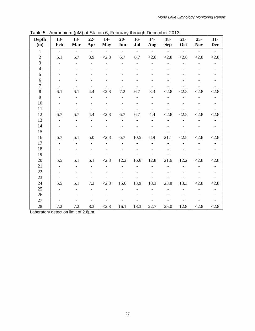
Table 5. Ammonium (µM) at Station 6, February through December 2013. .................. 27

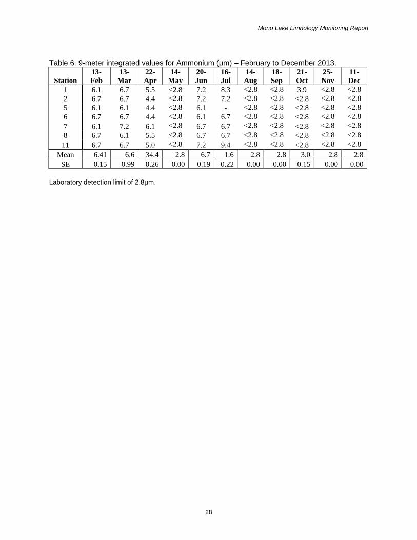
Table 6. 9-meter integrated values for Ammonium (µm) – February to December . ..... 28

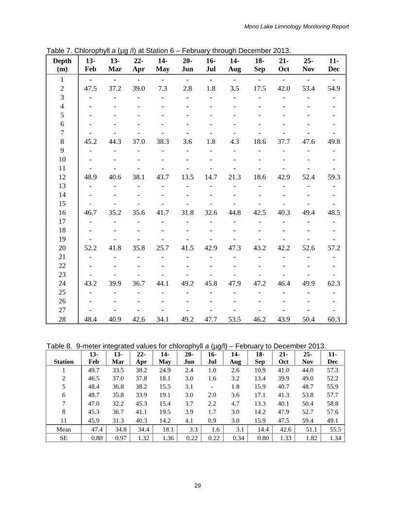
Table 7. Chlorophyll a (µg /l) at Station 6 – February through December 2013. ........... 29

Table 8. 9-meter integrated values for chlorophyll a (µg/l) – February to December . ... 29

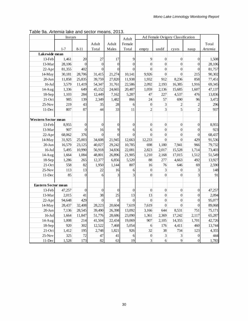
Table 9a-c. Artemia lake and sector means, 2013. ....................................................... 30

Table 10. Lakewide Artemia instar analysis, 2013. ....................................................... 33

Table 11. Artemia biomass summary, 2013. ................................................................. 34

Table 12. Artemia fecundity summary, 2013. ................................................................ 34

Table 13. Summary Statistics of Adult Artemia:1 May- 30 November, 1979-2013. ....... 35


3

LIST OF FIGURES

Figure 1. Sampling Stations at Mono Lake and Associated Station Depths. ................ 36

Figure 2. Mean daily and mean maximum 10-minute wind speed Paoha Island. ......... 37

Figure 3. Minimum and maximum daily temperature (°C ) at Paoha Island,. ............... 38

Figure 4. Mean relative humidity (%) – Paoha Island . ................................................. 39

Figure 5. Precipitation (mm) at Cain Ranch. ................................................................ 40

Figure 6. Surface elevation of Mono Lake and mixing regime, 1979-2013. .................. 41

Figure 7. Secchi depths (meters) and standard error, 2013. ........................................ 42

Figure 8. Temperature profiles at Station 6, February to December 2013. .................. 43

Figure 9. Conductivity (mS/cm) profiles at Station 6, April-December, 2013. ............... 44

Figure 10. Dissolved oxygen profiles at Station 6, February – December 2013. .......... 45

Figure 11. Ammonium profiles Station 6, February – December 2013. ........................ 46

Figure 12. Chlorophyll a profiles at Station 6, February – December 2013. ................. 47

Figure 13. Artemia reproductive parameter and fecundity, 2013. ................................. 48

Figure 14. Mean Lakewide Artemia abundance 1982-2013. ........................................ 49

Figure 15. Mean adult Artemia 1979-2013 vs. years subsequent onset of monomixis. 50

Figure 16. Mean surface elevation 1979-2013 vs.mean shrimp abundance ............... 51

Figure 17. Annual export of water vs.input to Mono Lake 1979-2013 . ........................ 52


4

INTRODUCTION

Limnological monitoring was conducted in 2013 at Mono Lake as required under the State

Water Resources Control Board Order No. 98-05. The limnological monitoring program at

Mono Lake is one component of the Mono Basin Waterfowl Habitat Restoration Plan (LADWP

1996). The purpose of the limnological monitoring program as it relates to waterfowl is to

assess limnological and biological factors that may influence waterfowl use of lake habitat

(LADWP 1996). The limnological monitoring program consists of four components:

meteorological, physical/chemical, phytoplankton, and brine shrimp population data.

An intensive limnological monitoring of Mono Lake has been funded by Los Angeles

Department of Water and Power (LADWP) since 1982. The Marine Science Institute (MSI),

University of California, Santa Barbara served as the principle investigator, and Sierra Nevada

Aquatic Research Laboratory (SNARL) provided field sampling and laboratory analysis

technicians up to July 2012. After receiving training in limnological sampling and laboratory

analysis methods from the scientists and staff at MSI and SNARL, LADWP Watershed

Resources staff assumed responsibility for the program, and has been conducting limnological

monitoring of Mono Lake since July of 2012.

This report summarizes monthly field sampling for the year of 2013. Laboratory support

including the analysis of ammonium and chlorophyll a in 2013 was provided by Environmental

Science Associates, Davis, California.

METHODS

Methodologies for both field sampling and laboratory analysis followed those specified in Field

and Laboratory Protocols for Mono Lake Limnological Monitoring (Field and Laboratory

Protocols) (Jellison, 2011). The methods described in Field and Laboratory Protocols are

specific to the chemical and physical properties of Mono Lake and therefore may vary from

standard limnological methods (e.g. Strickland and Parsons 1972). The methods and

equipment used by LADWP to conduct limnological monitoring was consistent and followed

those identified in Field and Laboratory Protocols except where noted below.

Meteorology

Two meteorological stations provided weather data in 2013 - Paoha Island and Cain Ranch.

The Paoha Island measuring station is located approximately 30 m from shore on the southern


5

tip of the island. The base of the station is at 1948 m above sea level, several meters above the

current surface elevation of the lake. Sensor readings are made every second and stored as

either ten minute averages or hourly values in a Campbell Scientific CR 1000 datalogger. Data

are downloaded to a storage module which is collected periodically during field sampling visits.

At the Paoha Island station, wind speed and direction (RM Young wind monitor) are measured

by sensors at a height of 3 m above the surface of the island and are averaged over a 10-

minute interval. During the ten minute interval, maximum wind speed is also recorded. Using

wind speed and direction measurements, the 10-minute wind vector magnitude and wind vector

direction are calculated. Hourly measurements of photosynthetically available radiation (PAR,

400 to 700 nm, Li-Cor 192-s), ten minute averages of relative humidity and air temperature

(Vaisalia HMP35C), and total rainfall (Campbell Scientific TE525MM-L tipping bucket) are also

stored. The minimum detection limit for the tipping bucket gage is 1 mm of water. The tipping

bucket is not heated therefore the instrument is less accurate during periods of freezing due to

sublimation of ice and snow. Paoha Island station precipitation data for 2013 will not be

reported due to the inaccuracy of measurements recorded (<6 mm total rainfall recorded).

The Cain Ranch meteorological station is located approximately 7 km southwest of the lake at

an elevation of 2088 m. This is an automated weather station managed by LADWP that records

daily minimum and maximum air temperature and precipitation. Precipitation data was recorded

in inches and is reported in millimeters for consistency with previous reports.

The daily mean wind speed, maximum mean wind speed, and relative humidity were calculated

from 10-minute averaged data from the Paoha Island site.

Field Sampling

Sampling of the physical, chemical and biological properties of the water including the Artemia

community was conducted at 12 buoyed stations at Mono Lake (Figure 1). The water depth at

each station at a lake elevation of 1,946 meters is indicated on Figure 1. Stations 1-6 are

considered western sector stations, and stations 7-12 are eastern sector stations. Surveys

were generally conducted around the 15th of each month.


6

Physical and Chemical

Sampling of the physical and chemical properties included lake transparency, water

temperature, conductivity, dissolved oxygen, and nutrients (ammonium). Lake elevation data

was obtained directly from the Mono Lake Committee website

(http://www.monobasinresearch.org/data/levelmonthly.php). Lake transparency was measured

at all 12 stations using a Secchi disk. A high-precision conductivity temperature-depth (CTD)

profiler (Idronaut,Model 316 Plus) was used to record water temperature and conductivity at

nine stations (2, 3, 4, 5, 6, 7, 8, 10 and 12). The CTD is programmed to collect data at 200

millisecond intervals. The CTD was lowered to the bottom at a rate of ~0.2 meters/second,

therefore data collection occurred at approximately 4 cm depth intervals.

Dissolved oxygen was measured at one centrally located station (Station 6). Dissolved oxygen

concentration was measured with a Yellow Springs Instruments Rapid Pulse Dissolved Oxygen

Sensor (YSI model 6562). Readings were taken at one-meter intervals throughout most of the

water column, and at 0.5 meter intervals in the vicinity of the oxycline or other regions of rapid

change. Data are reported for one-meter intervals only.

Monitoring of ammonium in the epilimnion was conducted using a 9-m integrated sampler at

stations 1, 2, 5, 6, 7, 8, and 11. An ammonium profile was developed by sampling at station 6

from eight discrete depths (2, 8, 12, 16, 20, 24, 28, and 35 meters) using a vertical Van Dorn

sampler. Samples for ammonium analyses were filtered through Gelman A/E glass-fiber filters

and following collection, immediately placed onto dry ice and frozen in order to stabilize the

ammonium content (Marvin and Proctor 1965). Ammonium samples were transported on dry

ice back to the laboratory transfer station. The ammonium samples were stored frozen until

delivered frozen to the University of California Davis Analytical Laboratory (UCDAL) located in

Davis, California. Samples were stored frozen until analysis.

Phytoplankton

Chlorophyll a sampling

Monitoring of chlorophyll a in the epilimnion was conducted using a 9-m integrated sampler at

stations 1, 2, 5, 6, 7, 8, and 11. A chlorophyll profile was developed by sampling at station 6

from seven discrete depths (2, 8, 12, 16, 20, 24, and 28 meters) using a vertical Van Dorn

sampler. Water samples were filtered into opaque bottles through a 120 µm sieve to remove all

http://www.monobasinresearch.org/data/levelmonthly.php


7

stages of Artemia. Chlorophyll a samples were kept cold and transported on ice back to the

laboratory transfer station located in Sacramento, CA.

Brine Shrimp

Artemia sampling

The Artemia population was sampled by one vertical net tow from each of twelve stations

(Figure 1). Samples were taken with a plankton net (0.91 m x 0.30 m diameter, 118 µm Nitex

mesh) towed vertically through the water column. Samples were preserved with 5% formalin in

Mono Lake water. When adults were present, an additional net tow was taken from four

western sector stations (1, 2, 5 and 6) and three eastern sector stations (7, 8 and 11) to collect

adult females for fecundity analysis including body length and brood size. Live females

collected for fecundity analysis were kept cool and in low densities during transport to LADWP

laboratory in Bishop.

Laboratory Analysis

Ammonium

Nitrogen is the primary limiting macronutrient in Mono Lake as phosphate is super-abundant

throughout the year (Jellison et al 1994 in Jellison 2011). External inputs are low, and vertical

mixing controls much of the annual internal recycling of nitrogen.

Starting in August 2012, the methodology used by UCDAL for ammonium was flow injection

analysis. In July 2012, this method was tested on high salinity Mono Lake water and was found

to give results comparable to previous years. This method has detection limits of approximately

2.8 µM. Immediately prior to analysis, frozen samples were allowed to thaw and equilibrate to

room temperature, and were shaken briefly to homogenize. Samples were heated with

salicylate and hypochlorite in an alkaline phosphate buffer (APHA 1998a, APHA 199b, Hofer

2003, Knepel 2003). EDTA (Ethylenediaminetetraacetic acid) was added in order to prevent

precipitation of calcium and magnesium, and sodium nitroprusside was added in order to

enhance sensitivity. Absorbance of the reaction product was measured at 660 nm using a

Lachat Flow Injection Analyzer (FIA), QuikChem 8000, equipped with a heater module.

Absorbance at 660 nm is directly proportional to the original concentration of ammonium, and

ammonium concentrations were calculated based on absorbance in relation to a standard

solution.


8

Chlorophyll a

Chlorophyll a is the most abundant form of chlorophyll found bound within the cells of the algae

comprising the phytoplankton community at Mono Lake. Chlorophyll a is therefore monitored as

an indicator of phytoplankton activity and abundance.

In 2013 the determination of chlorophyll a was done by fluorometric analysis following acetone

extraction. Fluorometry was chosen, as opposed to spectrophotometry, due to higher sensitivity

of the fluorometric analysis, and because data on chlorophyll b and other chlorophyll pigments

were not needed.

At the laboratory transfer station in Sacramento, water samples (200 mL) were filtered onto

Whatman GF/F glass fiber filters (nominal pore size of 0.7 µm) under vacuum. Filter pads were

then stored frozen until they could be overnight mailed, on dry ice, to the University of Maryland

Center for Environmental Science Chesapeake Biological Laboratory (CBL), located in

Solomons, Maryland. Sample filter pads were extracted in 90% acetone and then refrigerated

in the dark for 2 to 24 hours. Following refrigeration, the samples were allowed to warm to room

temperature, and then centrifuged to separate the sample material from the extract. The extract

for each sample was then analyzed on a fluorometer. Chlorophyll a concentrations were

calculated based on output from the fluorometer. Throughout the process, exposure of the

samples to light and heat was avoided.

The fluorometer used in support of this analysis was a Turner Designs TD700 fluorometer

equipped with a daylight white lamp, 340-500 nm excitation filter and >665 nm emission filter,

and a Turner Designs Trilogy fluorometer equipped with either the non-acid or the acid optical

module.

Artemia Population Analysis and Biomass

An 8x to 32x stereo microscope was used for all Artemia analyses. Depending on the density of

shrimp, counts were made of the entire sample or of a subsample made with a Folsom plankton

splitter. When shrimp densities in the net tows were high, samples were split so that

approximately 100-200 individuals were subsampled. Shrimp were classified as nauplii (instars

1-7), juveniles (instars 8-11), or adults (instars >12), according to Heath’s classification (Heath

1924). Adults were sexed and the reproductive status of adult females was determined. Non-

reproductive (non-ovigerous) females were classified as empty. Ovigerous females were


9

classified as undifferentiated (eggs in early stage of development), oviparous (carrying cysts) or

ovoviviparous (naupliar eggs present).

An instar analysis was conducted at seven of the twelve stations (Stations 1,2,5,6,7,8, and 11).

Nauplii at these seven stations were further classified as to specific instar stage (1-7). Biomass

was determined from the dried weight of the shrimp tows at each station. After counting,

samples were rinsed with tap water and dried in aluminum tins at 50°C for at least 48 hours.

Samples are weighed on an analytical balance immediately upon removal from the oven.

Artemia Fecundity

Immediately upon return to the laboratory, ten females from each sampled station were

randomly selected, isolated into individual vials, and preserved with 5% formalin. Female length

was measured at 8X from the tip of the head to the end of the caudal furca (setae not included).

Egg type was noted as undifferentiated, cyst, or naupliar. Undifferentiated egg mass samples

were discarded. Brood size was determined by counting the number of eggs in the ovisac and

any eggs dropped in the vial. Egg shape was noted as round or indented.

Artemia Population Statistics

Calculation of long-term Artemia population statistics followed Jellison and Rose (2011). Daily

values of adult Artemia between sampling dates were linearly interpolated in Microsoft Excel.

The mean, median, peak and centroid day (calculated center of abundance of adults) were then

calculated for the time period May 1 through November 30. Long-term values were determined

by calculating the mean, minimum and maximum values for these parameters for the time

period 1979-2013.

RESULTS

Meteorology

Wind Speed, relative humidity, air temperature and precipitation data from the weather station at

Paoha Island are summarized monthly for 2013. Precipitation data from the weather station at

Cain Ranch is summarized monthly.

Wind Speed and Direction

Mean daily wind-speed varied from 0.85 to 9.54 m/sec with an overall mean for this time period

of 3.2 m/sec (Figure 2). The daily maximum 10-min averaged wind speed on Paoha Island


10

averaged 1.5 times the mean daily wind speed. The maximum recorded 10-min reading of 13.4

m/sec occurred on the afternoon of March 6th. As has been case in previous years, winds were

predominantly from the south (mean 187 degrees).

Air Temperature

Daily air temperatures as recorded at Paoha Island ranged from a low of -11.4°C on January 13,

2013 to a high of 24.4°C on July 20 (Figure 3). Winter temperature (January through February)

ranged from -8.5°C to 3.4°C with an average maximum daily temperature of 3.4°C. The

average maximum daily summer temperature (June through August) was 26.8°C.

Relative Humidity and Precipitation

The mean relative humidity for the period January 1st – December 31st, 2013 was 54% (Figure

4). Mean relative humidity was negatively correlated with both daily mean wind speed (r = -

0.482, p<0.001, n=365), and maximum 10-minute mean wind speed (r = -0.470, p<0.001,

n=365). The total precipitation measured at Cain Ranch was 87.9 mm. Winter month

precipitation was modest but increased in spring with April rainfall of 13 mm and 11.2 mm in

May (Figure 5). The largest rain event produced 12.4 mm of rain on September 22ndth. Both

total amount of rain (15 mm) and frequency of rain events (6) were greatest in July. The end of

the 2013 was dryer producing less than 6 mm of rainfall in November and about 1.8 mm in

December.

Physical and Chemical

Surface Elevation

The surface elevation of Mono Lake in January 2013 was 6382.0 feet. A slight increase in

elevation to 6382.2 feet was observed in April. Starting in May lake elevation declined and

continued through December. From the 2013 high of 6382.2 feet in April, the lake dropped a

total of 1.8 feet to a low of 6380.4 feet by December 11th. Figure 6 shows lake elevation 1979

through 2013 and the mixing regime observed each year. As will be discussed below, Mono

Lake continued to exhibit a monomictic mixing regime in 2013. For 2013 the greatest change is

surface elevation (0.4 feet) occurred in late summer from August to September and early fall

from September to October.


11

Transparency

The lowest spring secchi (average) depth was 0.38 m +/- 0.02 mm in April (Table 1, Figure 7).

Secchi depth increased through mid-May when transparency was 1.15 m +/- 0.12 m. As

Artemia grazing reduced midsummer phytoplankton, lakewide transparency increased to a

maximum of 5.08 m +/- 0.2 m in July. Secchi depths began to decrease through the fall, and

remained between 0.57 m and 0.66 m from October through December.

Water Temperature

The water temperature data from Station 6 indicate that Mono Lake remained meromictic in

2013 as the lake was thermally stratified from late spring to early fall with turnover occurring

once later in the fall (Table 2, Figure 8). In April the thermocline began to form at 9-10 m (as

indicated by the greater than 1°C change per meter depth) and fluctuated between 9 and 11 m

through August before deepening to 15 m by September. In October temperatures began to

cool and stratification weakened as temperatures throughout the water column differed by less

than 1˚C. By the late November survey temperatures were fairly isothermic from 1 m to 40 m

indicating the onset of holomixis (Table 2, Figure 8). Holomixis persisted throughout December

as temperature data indicate little change with water temperatures at 6.3°C from 2 meters

gradually declining to 5.2°C at 39 m.

Dissolved Oxygen

Dissolved oxygen (DO) levels at Station 6 were indicative of historical limnological mixing

patterns observed at Mono Lake. In 2013 Mono Lake had one period of fall turnover marking

the 2nd continuous year of monomictic conditions. DO concentration in winter/spring months

within the first 15 m of the water column ranged as low as 5.8 mg/l in April to as high as 13.6

mg/l in May (Table 4, Figure 10). In May DO levels in the first 6 m of the water column were

about twice as high (12.9 mg/l) as 2012 levels (6.1 mg/l). Dissolved oxygen levels at Mono

Lake are typically higher in spring months as phytoplankton blooms follow increased sunlight

and temperature levels. DO levels near the lake substrate (39m) decreased from February to

May (7.1 to 1.8 mg/l) prior to the onset of meromixis. In June, Mono Lake began to thermally

stratify with meromictic conditions persisting through August. In September the thermocline

began to slowly breakdown prior to holomixis. In the fall epilimnetic DO concentrations were

highest in September (9.3 mg/l) followed by October (3.1 mg/l) and were lowest in November

(1.0 mg/l) as monomolimnetic hypoxic waters fully mixed with epilimnetic waters (Table 4,

Figure 10). Mono Lake remained monomictic in December.


12

Conductivity

Conductivity data was collected from the CTD field sampling device on a monthly basis. In situ

conductivity measurements were corrected for temperature (25˚C) and reported at one meter

intervals beginning at one meter in depth down to the lake bottom. Conductivity data is used to

evaluate the salinity profile of the lake and are reported in Table 3. Data from February and

March are not reported due to malfunction of the CTD probe. The winter of 2013 marked the

second consecutive year of monomixis at Mono Lake. Mono Lake surface elevation slowly

increased in the beginning of 2013 and reached its peak in April as freshwater inputs from

snowmelt likely contributed to vertical salinity stratification. Specific conductivities for April

ranged from 83.6 to 85.9 mS/cm in the epilimnion and from 88.1 to 89.5 mS/cm below 14

meters (Table 3).

As thermal and chemical stratification became more prominent in the summer months the

greatest difference between epilimnetic and hypolimnetic specific conductivities were reported in

July and August (Table 3, Figure 9). For August specific conductivity averaged 78.8 mS/cm in

the epilimnion and 87.7 mS/cm in the hypolimnion. By October as the thermocline became less

defined (<1˚C temp difference per meter) average specific conductivity was only 0.8 mS/cm

different between the epilimnion (85.4 mS/cm) and hypolimnion (86.2 mS/cm). By late

November as Mono lake became holomictic specific conductivity varied the least throughout the

water column (0.4 mS/cm, Table 3, Figure 9).

Ammonium

Ammonium levels were uniform throughout the water column in early 2013 (Table 5, Figure 11)

due to holomixis that occurred in late 2012. Ammonium levels in February and March of 2013

(24 m and below) as measured at Station 6 ranged from 5.5 to 7.2 µM. Commensurate with

increased algal growth, ammonium levels declined throughout the water column into April and

were below the detection limit in May (<2.8 µM). Epilimnetic ammonium levels increased in

June and July as Artemia abundance increased and excretion of fecal pellets raised the

ammonium levels in the water column. The July through October period had large increases in

the level of ammonium in the hypolimnion below approximately 20 m (12.2 to 25 µM). Increases

in the ammonium concentration in the hypolimnion during these months is associated with

increases in algal debris and Artemia fecal pellets as these waste products sink to the bottom

and decompose (Jellison 2011). Under anoxic conditions during summer thermal stratification

ammonium concentrations tend to be higher at the sediment-water interface as bacterial


13

nitrification ceases and the adsorptive capacity of the sediments is greatly reduced due to loss

of the oxidized microzone (Wetzel, 2001). Ammonium was below the detection limit (<2.8 µM)

and well-mixed throughout the water column by November and mixing remained complete

through mid-December. This reduction in ammonium levels throughout the water column

coincides with holomixis and increased uptake by phytoplankton as predation pressure from

Artemia decreases in winter months.

Phytoplankton

Seasonal changes were noted in the phytoplankton community, as measured by chlorophyll a

concentration (Tables 7 and 8, Figure 12). On the February survey, epilimnetic chlorophyll

levels averaged 47.4 µg/L (Table 8). Within the epilimnion, lakewide mean chlorophyll values

decreased through the spring and reached their lowest point in the middle of summer (1.6 µg/L,

Table 8). As the lake began to stratify in late spring and zooplankton grazing increased,

chlorophyll levels reduced from 38.3 µg/L in May, to 3.6 µg/L in June at 8 meters in depth (Table

7). In August chlorophyll concentrations varied from 3.5 µg/L at 2 meters to 53.5 µg/L at 28

meters in the hypolimnion. By October as the water column began to fully mix the lakewide

epilimnionic average had increased to 42.6 µg/l and reached its peak in December at 55.5 µg/L

(Table 8). Overall both the lakewide trends (Table 8) and discrete sampling at Station 6 (Table

7) indicate changes in chlorophyll concentrations closely follow turnover conditions and

fluctuations in grazing pressure from population changes of brine shrimp.

Brine Shrimp

Artemia Population Analysis and Biomass

Artemia population data is presented in Tables 9a through 9c as lakewide means, sector means

associated standard errors and percentage of population by age class. As discussed in

previous reports (Jellison and Rose 2011), zooplankton populations can exhibit a high degree of

spatial and temporal variability. In addition, when sampling, local convergences of water

masses may concentrate shrimp above overall means. For these reasons, Jellison and Rose

have cautioned that the use of a single level of significant figures in presenting data is

inappropriate, and that the reader should always consider the standard error associated with

Artemia counts when making inferences from the data.


14

Artemia Population

Hatching of overwintering cysts had already initiated by February as the mid-February sampling

detected an instar lakewide mean abundance of 1,481 +/- 312/m2. The overwhelming majority

(96.9%) of the instars in mid-February were instar 1. Instar abundance increased through mid-

April to a peak of 81,757 +/- 13,273/m2 which was twice the density of April 2012 counts.

Similar to 2012 in early spring adults continued to be essentially absent. The 2013 peak

Artemia lakewide abundance of 90,302 +/-18,865/m2 was recorded on the May 14 survey. By

May, adults comprised approximately 34% of the Artemia population. The instar analysis

indicated a diverse age structure of instars 1-7 and juveniles (instars 8-11) in May. In June,

females with cysts were first recorded. By July females with cyst abundance peaked at 16,385

+/- 2,509/m2 and by August reproduction decreased significantly, with instars and juveniles

comprising only 4.2% of the population. The greatest summer adult Artemia abundance

occurred in July (54,347+/-8,198/m2). The adult population declined in August (45,152 +/-

8,509/m2) with a much greater reduction by September (12,449 +/- 1,257/m2). In mid-October,

adult shrimp numbered 2,349 +/- 338/m2, dropping to a low of 35 +/- 9/m2 in November and 44

+/- 16/m2 in December.

Instar Analysis

The instar analysis, conducted at seven stations, showed patterns similar to those shown by the

lakewide and sector analysis, but provide more insight into Artemia reproductive cycles

occurring at the lake (Table 10). Instars 1 and 2 were most abundant in February and March as

overwintering cysts were hatching. In April various age classes of instars 1-7 and juveniles

were present and comprised approximately 99.5% of the Artemia population. In May a diverse

age structure of instars was present, while adults comprised 34.8% of all Artemia. The number

of instar 1 increased again in June indicating a second generation of reproduction. By June

juvenile and instar abundance represented about 50% of the age structure population. The

presence of late stage instars and juveniles indicate survival and recruitment into the population.

Instar and juvenile abundance decreased to 21.6% in July and reached a low of 4.2% of the

Artemia population. Adult abundance decreased from 90% in September to 4.7% in December

while instar and juvenile age classes increased from 10% to near 95% over the same period.

While proportions of Artemia age classes changed over the year, adult, juvenile and instar

abundances declined considerably in November and December as anticipated (Table 9a).


15

Biomass

Mean Artemia biomass values were low in February and March, ranging from 0.14 gm/m2 in

February to 1.80 gm/m2 in March (Table 11). Mean lakewide Artemia biomass peaked at 28.58

gm/m2 in mid-July, and remained fairly level through August, at 23.85 gm/m2 before declining in

September to14.98 gm/m2. By October, mean lakewide biomass had declined to 3.64 gm/m2,

and was minimal in November and December. Biomass values differed between western and

eastern sectors seasonally as early spring (March and April) biomass was higher in the east,

and early fall values (August-Sept) were slightly higher in the west. In July during peak shrimp

abundance biomass values were higher in the east at 22.39 gm/m2 compared to 14.37 gm/m2 in

the west.

Reproductive Parameters and Fecundity Analysis

Table 12 and Figure 13 show the result of the fecundity analysis and lakewide reproductive

parameters. In May, no ovigery was detected. In June approximately 84% of females were

ovigerous, with 69% oviparous (cyst-bearing), 7.2% ovoviviparous (naupliar eggs) and 7.6%

undifferentiated eggs (Table 9c). From July through October, over 90% of females were

ovigerous with the majority (72-86%) oviparous. Ovovivipary was over 10% in both October

(11%) and December (14%).

The lakewide mean fecundity showed pronounced seasonal variation. The lakewide mean

fecundity was initially 24.2 +/- 0.9 eggs per brood in mid-June, decreasing slightly to 17.6 +/- 0.6

eggs per brood in July (Table 12). Lakewide fecundity was 69.1 +/- 2.9 eggs per brood in

September and reached a high of 93.7 +/- 4.3 eggs per brood in October. The majority of

fecund females (91-100%) were oviparous, while ovoviviparous females with naupliar eggs

constituted the remainder. Little difference was observed in fecundity between the western and

eastern sectors. The minimum mean female length was 8.9 mm in July which corresponded

with the smallest mean brood sizes for the year. The largest females (mean 10.9 mm) were

recorded in October when mean brood size was also at its highest for the year (93.7). The

number of indented cysts remained relatively constant near 50% with a high of 66% in July

(Table 12).

Artemia Population Statistics

The calculated seasonal peak in adult Artemia of 54,347/m2 was above the long-term average of

45,694/m2 (Table 13). The mean and median were also above average (26,033 vs. 19,775/m2


16

and 31,275 vs 18,574/m2). The centroid is the calculated center of abundance of adults. The

centroid day of 196 in 2013 corresponds to July 15th. The long-term mean centroid day for the

time period 1979-2013 is 211 (July 29). Figure 14 shows daily lakewide mean adult Artemia

values for 1982-2013. Adult Artemia numbers were the second highest ever recorded for July in

2013 and moderate through fall. In contrast, 2012 adult numbers peaked in May and were the

second lowest ever recorded in July (Figure 14). In 2013, mean adult abundance was the 6th

highest ever recorded. Interestingly 2013 was the first year since the most recent episode of

meromixis in 2011 that ammonium previously contained in the hypolimnion was fully available

for phytoplankton. The year 2012 marked the 4th time that Mono Lake shifted from meromixis to

monomixis during the period of record. There is data to suggest that years following the onset

of monomixis have coincided with high adult Artemia abundance at Mono Lake (Figure 15). The

long term data show 1989 and 2004 as the 2nd and 3rd highest adult density recorded from

1979-2013 (Table 12, Figure 14). The longest periods of meromixis, 1983-1987 and 1995-2002

ended just previous to these years (see Figure 6).

DISCUSSION

Thermal and Chemical Stratification

In 2013, Mono Lake experienced a net reduction in elevation of 1.6 feet and holomixis or

complete autumn mixing for the second year in a row. Following winter holomixis, thermal

stratification became evident as early as April and strong thermal stratification was present by

June. Thermal stratification was observed as late as September. By November an isothermal

water column was present indicating full mixing of the water column.

Conductivity data indicated the establishment of a salinity gradient beginning in April with the

greatest difference in specific conductivity in the epilimnion and hypolimnion occurring in July

and August. In November conductivity measurements were most consistent throughout the

water column during holomixis and were greatest on average in December likely attributable to

decreased lake volume.

Dissolved Oxygen The dissolved oxygen values followed the seasonal pattern generally observed at Mono Lake.

DO values were highest in spring during algal blooms, but decreased noticeably in the summer

throughout the water column. Increasing water temperatures lead to decreases in dissolved

oxygen as the concentration of oxygen in solution is inversely proportional to temperature.


17

Increases in Artemia populations also decrease algal populations, thereby decreasing oxygen

production. As algal populations likely recovered in the fall due to decreasing shrimp numbers,

dissolved oxygen values in the epilimnion increased. Stratification of the lake through the

summer results in a depletion of oxygen beneath the thermocline. When mixing occurs, further

depletion of oxygen in the water column may occur as water in the oxic epilimnion is mixed with

the anoxic hypolimnetic water, and consumed by biological oxygen demand in the

monimolimnion (Jellison and Rose 2011). This was evident during November and December

sampling when oxygen values were low throughout the water column as deep mixing was

occurring.

Ammonium and Chlorophyll Ammonium sampling further supports the presence of a monomictic lake regime in 2013. Prior

to summer stratification ammonium concentrations were similar throughout the water column.

The June through October period showed large increases in the level of ammonium in the

hypolimnion below approximately 20 m, as algal debris and Artemia fecal pellets accumulated

and decomposed in the hypolimnion. In addition, in the anoxic hypolimnion internal loading

occurs as ammonium released from the sediments further increases ammonium levels.

Ammonium concentrations were low (below detection limit) throughout the water column by mid-

November and mixing remained complete through mid-December. Low levels of ammonium in

winter months coincided with the greatest concentration of mean chlorophyll in the epilimnion

across all stations sampled and throughout the water column at station 6.

Epilimnetic chlorophyll levels were initially moderate from February through April and decreased

almost 50% in May coincident with the increase in shrimp numbers and subsequent decreases

in the algal population. Mean epilimnetic chlorophyll levels were lowest in July coinciding with

peak adult Artemia abundance. As shrimp numbers declined in early fall, by mid-October,

chlorophyll levels were nearly recovered to February 2013 levels.

Brine Shrimp Mean adult Artemia abundance was almost 60% higher in 2013 compared to 2012, although

peak adult abundance was only slightly higher (Table 13). Total brine shrimp numbers (adults

and instars) peaked in May and were fairly evenly represented by early and late stage instars

and adult Artemia (Table 9a). Adult abundance peaked in July which was more representative

of the long term trend as compared to the previous sampling year (Figure 14). The centroid


18

peak in abundance occurred on July 15th which was 15 days earlier than the long term mean.

Peak early instar abundance occurred in April representing more than 50% of early stage

instars for the year (Table 9a). Recruitment of early instars to the population was evident by

increasing late stage instars in May and June and peak adult numbers in July. Mean biomass

was greatest in summer months reaching its peak in July (Table 11). Shrimp numbers

remained steady through fall and were moderate into October as compared to long-term data.

A high rate of ovigery and high brood numbers were observed in early fall. Long-term

parameters indicate an above average seasonal peak in adult Artemia with mean abundance

32% greater than the long term mean (Table 13).

Recent Period of Monomixis and Importance to Biota The health of Artemia populations are linked to primary food sources such as phytoplankton.

The main nutrients required by phytoplankton are nitrogen and phosphorous. In Mono Lake

nitrogen and its external inputs are limited but phosphorous is abundant. The majority of

nitrogen biologically available for direct uptake by phytoplankton is in the form of ammonium. In

Mono Lake ammonium is the limiting nutrient for primary productivity and relative contributions

from internal nutrient cycling and brine shrimp have been documented (Jellison and Melack

1986, 1988). Ammonium bound in the sediments is made available by internal nutrient

recycling driven by changes in thermal and chemical density stratification of Mono Lake.

Historically, Mono Lake has shifted between meromictic and monomictic conditions dependent

on a multitude of factors including climatic conditions such as temperature, evaporation, wind,

freshwater inputs from precipitation and runoff and diversions. All of these influences affect

stratification and mixing dynamics of Mono Lake. Mono Lake exhibited a monomictic mixing

regime from 2008-2010, was meromictic in 2011, returned to monomixis in 2012 and remained

so in 2013. Monomixis, or annual mixing once a year, is important to the nutrient cycle at Mono

Lake as it returns nutrients, most importantly, ammonium back to the epilimnion for use by

phytoplankton.

Historic Shifting from Meromictic to Monomictic Conditions Analysis of long term mixing regimes at Mono Lake is important as water column mixing and

internal nutrient cycling affect biota including Artemia population dynamics. As stated previously

the most recent episode of monomixis (2012-2013) marks the 4th time since 1982 that Mono

Lake has shifted from a meromictic to a monomictic state. Although vertical mixing does not

provide the sole source of ammonium in Mono Lake, it is especially important for primary


19

producers in the spring and fall as contributions from Artemia excretions are greatly reduced

(Melack, 1988, Jellison and Melack, 1993). Artemia populations have greatly fluctuated since

LADWP began monitoring Mono Lake in 1982 (see Table 13, Figure 14). Historically Artemia

abundance has been high in years following the onset of monomixis including 1989, 2004, 2009

and 2013 (Figure 15). Ammonium liberated from anoxic sediments is made biologically

available to plankton the fall and winter (1st year of monomixis) previous to years when annual

Artemia abundance peaks have occurred. Perhaps an abundance of primary production in the

year following breakdown of meromixis allow brine shrimp populations to peak the subsequent

spring and summer as evidenced by high abundance in those years. Jellison and Rose report

high values for primary production in those years following the breakdown of meromixis (2011),

although there are occurrences when primary production was high during the calendar year of

meromixis (Jellison and Rose, 2011). Studies have shown that spring generation brine shrimp

raised at high food densities develop more quickly, begin reproducing earlier and that

abundance of algae may likely affect year to year changes in shrimp abundance (Jellison and

Melack, 1993).

While availability of food sources and nutrients are important they do not fully determine year to

year abundance of Artemia (subsequent to meromixis). The unique life history of female brine

shrimp allow for dormant cysts to stay viable for years. It is known that diapausing cysts require

oxygen for hatching (Lenz, 1984). Under meromictic conditions when much of sediment has

been anoxic for multiple years a large percentage of cysts likely fail to hatch. When sediments

finally become reoxygenated during monomixis dormant cysts may begin to hatch (Jellison et al.

1989). The combination of reoxygenated dormant cyst hatching and mixing of ammonium rich

water may likely explain peak years in adult brine shrimp abundance following long periods of

meromixis.

Mono Lake Volume and Changes from Fluctuation in Freshwater Inputs

When evaluating the mean surface elevation from 1979 to 2013 a pattern may be emerging

between declining lake elevation and annual brine shrimp abundance. The greatest mean adult

shrimp density documented since 1979 occurred in 1982 when mean annual surface elevation

was at the lowest recorded level in the past 34 years (Figure 15, Figure 16). During the

preceding years water exports were high resulting in minimal release to Mono Lake (Figure 17).

This year (1982) was subsequent to a period of several years of monomixis and was followed

by a large release of freshwater in 1983 which set up conditions for a 5 year period of


20

meromixis. The 2nd and 3rd highest mean adult Artemia densities occurred in 1989 and 2004

which are years subsequent to the breakdown of meromixis. These were years following below

normal runoff years resulting in declining lake levels due to decreased freshwater input. The

reduced lake volume combined with reduced fresh water input lessens the thermal and

chemical gradient between the upper and lower water column and Mono Lake begins to mix.

There may be a long term pattern of population booms during periods of transition from low to

high lake levels or more importantly periods following the breakdown of meromixis (Figure 15,

Figure 16). Despite the benefits from the release and circulation of ammonium rich water during

initial years post meromixis, adult brine shrimp populations greatly reduce the following years

during both monomictic and meromictic periods (Figure 15).


21

REFERENCES

American Public Health Association (APHA). 1998a. Method 4500-NH3 H. Flow Injection Analysis (PROPOSED) in Standard Methods for the Examination of Water and Wastewater, 20th Edition. Clesceri, L. S., Greenberg, A. E., and Eaton, A. D., eds. Washington DC; 1998. pp. 4-111 – 4-112.

American Public Health Association (APHA). 1998b. Method 4500-NO3 I. Cadmium Reduction Flow Injection Method (Proposed) in Standard Methods for the Examination of Water and Wastewater, 20th Edition. Clesceri, L. S., Greenberg, A. E., and Eaton, A. D., eds. Washington DC; 1998. pp. 4-121 - 4-122.

Hofer, S. 2003. Determination of Ammonia (Salicylate) in 2M KCl soil extracts by Flow Injection Analysis. QuikChem Method 12-107-06-2-A. Lachat Instruments, Loveland, CO.

Heath, H. 1924. The external development of certain phyllopods. J. Morphology. 38: 453-83.

Jellison, R. J. 2011. Field and Laboratory Protocols for Mono Lake Limnological Monitoring. Marine Sciences Institute. University of California, Santa Barbara.

Jellison, R. and K. Rose. 2011. Mixing and Plankton Dynamics in Mono Lake, California. Marine Sciences Institute. University of California, Santa Barbara.

Jellison, R. and J.M. Melack. 1993. Algal photosynthetic activity and its response to meromixis

in hypersaline Mono Lake, California. Vertical mixing and density stratification during onset, persistence and breakdown of meromixis. Limnol.Oceanogr. 38:818-837.

Jellison, R. and J.M. Melack. 1986. Nitrogen supply and primary production in hypersaline Mono

Lake. Trans. Am. Geophys. U. 67:974. Jellison, R. and J.M. Melack. 1988. Photosynthetic activity of phytoplankton and its relation to

environmental factors in hypersaline Mono Lake, California. Trans. Am. Geophys. U. 67:974. Jellison, R. G.L. Dana, and J.M. Melack. 1989. Phytoplankton and brine shrimp dynamics in

Mono Lake, California. Annual report to the Los Angeles Department of Water and Power.

Knepel, K. 2003. Determination of Nitrate in 2M KCl soil extracts by Flow Injection Analysis. QuikChem Method 12-107-04-1-B. Lachat Instruments, Loveland, CO.

Lenz, P.H. 1984. Life-history of an Artemia population in a changing environment. Journal of Plankton Research 6(6):967-983.

Los Angeles Department of Water and Power (LADWP). 1996. Mono Basin Waterfowl Habitat Restoration Plan. Prepared for the State Water Resources Control Board. In response to Mono Lake Basin Water Right Decision 1631.


22

Marvin, K. T. and Proctor, R. R. 1965. Stabilizing the ammonia nitrogen content of estuarine and coastal waters by freezing. Limnolol. Oceanogr. Vol 10. pp. 288-90.

Melack, J.M. 1988. Limnological conditions in Mono Lake, California: review of current

understanding. In: Final reports from subcontractors, The Future of Mono Lake: Reports on the CORI study of the University of California, Santa Barbara, For the legislature of the State of California. University of California, Santa Barbara.

Strickland, J.D.H., and T.R. Parsons. 1972. A practical handbook of seawater analysis. Bulletin 167 (2nd ed.). Fisheries Research Board of Canada, Ottawa, Canada.

Wetzel, R.G. 2001. Limnology, Lake and River Ecosystems. (3rd ed.). Academic Press, San

Diego, California.


23

Table 1. Secchi Depths (m); February – December 2013.

STATION SAMPLING DATE

13-

Feb

13-

Mar

22-

Apr

14-

May

20-

Jun

16-

Jul

14-

Aug

18-

Sep

21-

Oct

25-

Nov

11-

Dec

Western Sector

1 0.40 0.60 0.40 0.70 2.80 6.10 4.80 2.10 0.60 0.45 0.7

2 0.60 0.60 0.40 0.65 3.50 5.50 5.50 1.80 0.70 0.55 0.8

3 0.50 0.55 0.30 0.95 2.80 5.30 4.40 1.70 0.60 0.65 0.7

4 0.50 0.55 0.40 1.00 2.20 4.90 4.00 1.30 0.60 0.6 0.7

5 0.60 0.55 0.45 1.00 2.50 4.50 5.50 1.50 0.60 0.6 0.75

6 0.45 0.70 0.40 0.90 2.40 4.30 4.10 1.40 0.50 0.5 0.7

AVG 0.51 0.59 0.39 0.87 2.70 5.10 4.72 1.63 0.60 0.56 0.73

SE 0.03 0.02 0.02 0.06 0.19 0.27 0.27 0.12 0.03 0.03 0.02

n 6 6 6 6 6 6 6 6 6 6 6

Eastern Sector

7 0.40 0.50 0.50 1.70 2.60 4.60 4.10 1.40 0.70 0.6 0.6

8 0.60 0.60 0.30 1.00 2.40 4.90 4.90 1.60 0.70 0.6 0.7

9 0.40 0.60 0.35 0.95 2.75 4.90 5.10 1.80 0.80 0.6 0.6

10 0.50 0.50 0.40 1.50 2.30 4.60 4.20 1.40 0.70 0.55 0.6

11 0.65 0.50 0.35 1.80 2.00 6.60 4.70 1.30 0.60 0.5 0.5

12 0.55 0.55 0.35 1.70 2.50 4.80 4.60 1.60 0.70 0.6 0.6

AVG 0.52 0.54 0.38 1.44 2.43 5.07 4.60 1.52 0.70 0.58 0.60

SE 0.04 0.02 0.03 0.15 0.11 0.31 0.16 0.07 0.03 0.02 0.03

n 6 6 6 6 6 6 6 6 6 6 6

Total Lakewide

AVG 0.51 0.57 0.38 1.15 2.56 5.08 4.66 1.58 0.65 0.57 0.66

SE 0.03 0.02 0.02 0.12 0.11 0.20 0.15 0.07 0.02 0.02 0.02

n 12 12 12 12 12 12 12 12 12 12 12


24

Table 2. Temperature (°C) at Station 6, February – December 2013.

Temperature (°C) at Station 6, February - December, 2013

Depth

(m)

13-

Feb

13-

Mar

22-

Apr

14-

May

20-

Jun

16-

Jul

14-

Aug

18-

Sep

21-

Oct

25-

Nov

11-

Dec

0 4.7 8.7 15.0 16.4 19.2 20.4 21.5 17.8 13.2 9.2 6.9

1 2.3 5.4 11.2 15.3 18.5 20.4 20.2 17.8 11.6 8.7 6.6

2 1.9 5.2 10.4 14.3 17.9 20.1 20.0 17.4 11.5 8.7 6.3

3 1.9 5.2 9.3 13.9 17.8 20.3 19.9 17.4 11.4 8.6 6.3

4 1.8 4.3 9.0 12.4 17.7 20.3 19.8 17.4 11.5 8.7 6.3

5 1.8 3.8 8.9 11.7 17.7 20.2 19.8 17.4 11.6 8.7 6.3

6 1.8 3.6 8.0 11.2 17.7 20.1 19.8 17.4 11.7 8.7 6.3

7 1.8 3.6 8.0 10.6 17.6 20.0 19.8 17.4 11.7 8.7 6.3

8 1.8 3.3 7.5 9.6 17.6 19.3 19.8 17.4 11.8 8.7 6.3

9 1.8 3.2 7.0 8.2 17.6 16.9 19.8 17.3 11.8 8.7 6.2

10 1.8 3.0 5.8 7.2 17.0 15.4 19.7 17.3 11.8 8.7 6.2

11 1.8 2.8 5.5 6.9 13.0 11.9 18.3 17.2 11.8 8.7 6.2

12 1.8 2.6 4.6 6.4 10.1 9.8 12.8 17.2 11.7 8.7 6.2

13 1.8 2.5 3.7 5.7 8.7 8.1 11.5 17.3 11.7 8.7 6.2

14 1.8 2.4 3.4 4.9 7.8 6.0 8.9 17.3 11.7 8.7 6.2

15 1.8 2.4 3.3 4.3 6.4 5.4 6.9 9.7 11.8 8.7 6.2

16 1.8 2.3 3.1 4.2 5.6 5.0 6.3 6.9 11.7 8.7 6.1

17 1.8 2.3 3.0 3.7 5.1 4.9 6.0 6.9 11.7 8.7 6.1

18 1.8 2.3 3.0 3.5 4.6 4.6 5.6 6.9 11.3 8.7 6.0

19 1.8 2.2 2.8 3.4 4.4 4.4 5.3 6.9 10.7 8.7 6.0

20 1.8 2.2 2.8 3.3 4.1 4.3 5.1 6.9 9.8 8.7 6.0

21 1.8 2.2 2.7 3.3 3.9 4.2 4.7 6.9 9.3 8.7 5.9

22 1.8 2.2 2.6 3.3 3.7 4.2 4.5 6.8 9.4 8.7 5.9

23 1.8 2.2 2.6 3.2 3.7 - 4.4 6.3 9.6 8.7 5.9

24 1.8 2.2 2.6 3.1 3.6 - 4.2 6.3 9.6 8.7 5.9

25 1.8 2.1 2.6 3.1 3.6 - 4.1 6.3 9.3 8.6 5.9

26 1.8 2.1 2.6 3.0 3.6 - 4.0 6.3 9.3 8.6 5.9

27 1.8 2.1 2.5 2.8 3.4 - 4.0 6.3 9.6 8.6 5.8

28 1.8 2.0 2.5 2.8 3.4 - 3.9 6.0 9.7 8.6 5.8

29 1.7 2.0 2.4 2.7 3.4 - 3.9 5.7 9.6 8.5 5.7

30 1.7 2.0 2.4 2.7 3.3 - 3.9 5.7 9.5 8.5 5.7

31 1.7 2.0 2.4 2.7 3.3 - 3.8 5.5 9.3 8.4 5.6

32 1.8 2.0 2.4 2.6 3.2 - 3.8 5.5 9.2 8.4 5.5

33 1.8 2.0 2.4 2.6 3.1 - 3.7 5.4 8.9 8.3 5.5

34 1.8 2.0 2.4 2.6 3.1 - 3.7 - 8.6 8.3 5.5

35 1.7 2.0 2.4 2.6 3.1 - 3.7 - 8.6 8.3 5.4

36 1.7 2.0 2.4 2.6 3.1 - 3.7 - - 8.2 5.3

37 1.7 2.0 2.4 2.6 3.0 - 3.6 - - 8.3 5.3

38 1.7 2.0 2.4 2.6 3.0 - 3.6 - - 8.2 5.2

39 1.8 2.0 2.4 2.6 3.0 - 3.6 - - 8.1 5.2

40 1.9 2.0 - - 3.1 - 3.6 - - 8.1 5.5

Temperature data is from YSI temperature-oxygen meter.


25

Table 3. Conductivity (mS/cm -1at 25°C) at Station 6, April – December 2013.

Depth

(m)

22-

Apr

13-

May

20-

Jun

16-

Jul

14-

Aug

18-

Sep

21-

Oct

25-

Nov

11-

Dec

1 83.6 82.7 82.0 78.1 77.6 83.0 85.1 86.7 88.0

2 84.0 82.6 82.9 78.5 78.7 83.7 85.3 86.8 88.1

3 84.1 81.9 83.0 78.0 78.9 83.8 85.4 86.8 88.1

4 85.0 83.4 83.1 78.2 79.0 83.8 85.4 86.8 88.2

5 85.1 83.8 83.2 78.3 79.0 83.8 85.4 86.7 88.2

6 85.0 84.5 83.3 78.4 79.0 83.8 85.4 86.8 88.2

7 85.3 84.0 83.2 78.5 79.0 83.8 85.4 86.7 88.2

8 85.5 84.5 83.1 79.7 79.0 83.9 85.4 86.7 88.2

9 85.9 84.5 83.2 80.3 79.0 83.9 85.4 86.7 88.2

10 86.1 85.6 84.0 82.7 79.4 84.0 85.4 86.7 88.2

11 86.4 86.0 84.9 83.3 81.2 84.0 85.5 86.8 88.2

12 86.2 86.5 85.1 84.6 84.3 84.1 85.4 86.8 88.2

13 88.1 86.5 85.4 85.6 84.5 84.1 85.5 86.8 88.2

14 88.5 87.4 86.2 86.4 85.4 80.1 85.5 86.8 88.3

15 88.6 87.9 86.8 86.8 86.6 87.1 85.5 86.8 88.3

16 89.0 88.2 87.4 87.3 86.6 86.7 85.5 86.8 88.4

17 89.0 88.5 87.6 87.7 86.6 86.7 85.6 86.8 88.4

18 89.0 88.5 87.9 87.7 87.1 86.7 85.8 86.8 88.4

19 89.1 88.5 88.2 88.1 87.3 86.7 86.3 86.8 88.4

20 89.1 88.6 88.2 87.8 87.5 86.7 86.1 86.8 88.4

21 89.2 88.6 88.3 87.9 87.7 86.9 86.1 86.8 88.5

22 89.2 88.7 88.3 88.0 87.8 86.9 86.0 86.8 88.5

23 89.2 88.8 88.4 88.1 87.9 86.9 85.9 86.8 88.5

24 89.2 88.9 88.4 88.2 88.0 87.1 86.1 86.9 88.5

25 89.3 88.9 88.5 88.3 88.2 86.9 86.2 86.9 88.5

26 89.4 89.0 88.6 88.4 88.1 86.7 86.1 86.9 88.6

27 89.4 89.0 88.6 88.5 88.1 87.2 86.1 86.9 88.6

28 89.4 89.1 88.6 88.4 88.2 87.3 86.1 86.9 88.6

29 89.4 89.1 88.7 88.4 88.2 87.3 86.2 86.9 88.7

30 89.4 89.1 88.7 88.4 88.3 87.3 86.2 87.0 88.7

31 89.4 89.2 88.8 88.5 88.4 87.5 86.2 87.0 88.8

32 89.4 89.2 88.8 88.5 88.3 87.4 86.2 87.0 88.8

33 89.5 89.2 88.8 88.5 88.3 87.5 86.5 87.1 88.9

34 89.5 89.2 88.8 88.6 88.4 87.5 86.7 87.1 88.9

35 89.4 89.2 88.8 88.6 88.4 87.5 86.7 87.1 89.0

36 - 89.2 - - - 87.7 86.9 87.1 89.0

37 - - - - - - - - -

38 - - - - - - - - -

39 - - - - - - - - -

40 - - - - - - - - -


26

Table 4. Dissolved Oxygen (mg/l) at Station 6, February – December 2013.

Depth

(m)

13-

Feb

13-

Mar

22-

Apr

14-

May

20-

Jun

16-

Jul

14-

Aug

18-

Sep

21-

Oct

25-

Nov

11-

Dec

1 11.2 9.9 12.0 10.2 4.3 5.4 7.3 9.3 3.1 1.0 1.4

2 11.4 10.4 12.3 10.2 4.4 5.5 7.3 8.9 3.1 1.1 1.4

3 10.7 10.5 12.4 11.0 4.4 5.4 7.2 8.7 3.1 1.1 1.3

4 10.3 10.7 12.9 12.0 4.4 5.5 7.0 8.5 2.9 1.0 1.2

5 9.8 10.4 12.0 13.4 4.3 5.5 7.0 8.3 2.8 1.0 1.0

6 9.6 9.7 10.7 13.6 4.3 5.5 7.0 8.1 2.6 0.9 0.8

7 9.6 9.3 10.4 12.8 4.2 5.5 7.0 7.7 2.5 0.9 0.6

8 9.6 9.2 9.4 11.8 4.1 5.5 6.9 7.6 2.3 0.9 0.5

9 9.7 9.0 8.9 10.4 3.9 5.3 6.9 7.4 2.2 0.9 0.4

10 9.6 8.5 8.6 9.4 3.9 5.5 6.8 7.3 2.2 0.8 0.3

11 9.5 8.0 8.4 8.4 4.4 5.9 6.1 6.2 2.3 0.8 0.2

12 9.4 7.7 7.9 7.6 4.6 6.7 5.0 6.2 2.3 0.8 0.2

13 9.5 7.4 7.1 7.3 4.5 5.3 3.9 6.2 2.3 0.8 0.2

14 9.4 7.2 6.1 6.2 4.2 4.6 2.7 6.3 2.3 0.7 0.2

15 9.4 7.0 5.8 5.9 3.5 3.2 1.9 2.0 2.2 0.7 0.1

16 9.3 6.8 5.8 5.4 3.1 1.6 1.0 1.7 2.1 0.7 0.1

17 9.3 6.7 5.8 5.3 2.4 0.9 0.6 1.6 2.1 0.7 0.1

18 9.3 6.6 5.6 5.3 1.4 0.6 0.5 1.6 1.7 0.7 0.1

19 9.2 6.6 5.5 5.3 0.9 0.3 0.5 1.5 1.4 0.7 0.1

20 9.3 6.5 5.4 5.1 0.6 0.2 0.4 1.5 1.1 0.7 0.1

21 9.2 6.4 5.4 5.0 0.3 0.2 0.4 1.5 1.1 0.7 0.1

22 9.2 6.4 5.2 4.6 0.1 0.1 0.4 1.5 1.2 0.7 0.1

23 9.3 6.4 5.0 4.2 0.1 0.1 0.4 1.5 1.3 0.7 0.1

24 9.4 6.4 5.0 4.2 0.0 - 0.4 1.5 1.1 0.7 0.1

25 9.5 6.4 5.0 4.1 0.0 - 0.4 1.5 0.8 0.7 0.1

26 9.0 6.4 4.9 4.0 0.0 - 0.4 1.5 0.6 0.6 0.1

27 9.1 6.4 4.8 4.1 0.0 - 0.4 1.5 0.5 0.6 0.1

28 9.2 6.3 4.7 4.2 0.0 - 0.4 1.5 0.4 0.6 0.1

29 9.1 6.3 4.6 4.2 0.0 - 0.4 1.5 0.2 0.6 0.1

30 9.0 6.3 4.4 4.2 0.0 - 0.4 1.5 0.2 0.6 0.1

31 8.9 6.2 4.3 4.2 0.0 - 0.4 1.5 0.1 0.6 0.1

32 8.6 6.0 4.3 3.9 0.0 - 0.4 1.5 0.0 0.6 0.1

33 8.4 5.9 4.3 3.4 0.0 - 0.4 1.5 0.0 0.6 0.1

34 8.4 5.8 4.0 3.1 0.0 - 0.4 - 0.0 0.6 0.1

35 8.0 5.8 3.8 2.9 0.0 - 0.4 - 0.0 0.6 0.1

36 7.9 5.7 3.8 2.4 0.0 - 0.4 - - 0.6 0.1

37 7.8 5.7 3.8 2.1 0.0 - 0.4 - - 0.6 0.1

38 7.4 5.7 3.8 2.0 0.0 - 0.4 - - 0.6 0.1

39 7.1 5.7 3.7 1.8 0.0 - 0.4 - - 0.6 0.1

40 5.3 4.7 - - 0.0 - 0.4 - - 0.6 0.1


27

Table 5. Ammonium (µM) at Station 6, February through December 2013.

Depth

(m)

13-

Feb

13-

Mar

22-

Apr

14-

May

20-

Jun

16-

Jul

14-

Aug

18-

Sep

21-

Oct

25-

Nov

11-

Dec

1 - - - - - - - - - - -

2 6.1 6.7 3.9 <2.8 6.7 6.7 <2.8 <2.8 <2.8 <2.8 <2.8

3 - - - - - - - - - - -

4 - - - - - - - - - - -

5 - - - - - - - - - - -

6 - - - - - - - - - - -

7 - - - - - - - - - - -

8 6.1 6.1 4.4 <2.8 7.2 6.7 3.3 <2.8 <2.8 <2.8 <2.8

9 - - - - - - - - - - -

10 - - - - - - - - - - -

11 - - - - - - - - - - -

12 6.7 6.7 4.4 <2.8 6.7 6.7 4.4 <2.8 <2.8 <2.8 <2.8

13 - - - - - - - - - - -

14 - - - - - - - - - - -

15 - - - - - - - - - - -

16 6.7 6.1 5.0 <2.8 6.7 10.5 8.9 21.1 <2.8 <2.8 <2.8

17 - - - - - - - - - - -

18 - - - - - - - - - - -

19 - - - - - - - - - - -

20 5.5 6.1 6.1 <2.8 12.2 16.6 12.8 21.6 12.2 <2.8 <2.8

21 - - - - - - - - - - -

22 - - - - - - - - - - -

23 - - - - - - - - - - -

24 5.5 6.1 7.2 <2.8 15.0 13.9 18.3 23.8 13.3 <2.8 <2.8

25 - - - - - - - - - - -

26 - - - - - - - - - - -

27 - - - - - - - - - - -

28 7.2 7.2 8.3 <2.8 16.1 18.3 22.7 25.0 12.8 <2.8 <2.8

Laboratory detection limit of 2.8µm.


28

Table 6. 9-meter integrated values for Ammonium (µm) – February to December 2013.

Station

13-

Feb

13-

Mar

22-

Apr

14-

May

20-

Jun

16-

Jul

14-

Aug

18-

Sep

21-

Oct

25-

Nov

11-

Dec

1 6.1 6.7 5.5 <2.8 7.2 8.3 <2.8 <2.8 3.9 <2.8 <2.8

2 6.7 6.7 4.4 <2.8 7.2 7.2 <2.8 <2.8 <2.8 <2.8 <2.8

5 6.1 6.1 4.4 <2.8 6.1 - <2.8 <2.8 <2.8 <2.8 <2.8

6 6.7 6.7 4.4 <2.8 6.1 6.7 <2.8 <2.8 <2.8 <2.8 <2.8

7 6.1 7.2 6.1 <2.8 6.7 6.7 <2.8 <2.8 <2.8 <2.8 <2.8

8 6.7 6.1 5.5 <2.8 6.7 6.7 <2.8 <2.8 <2.8 <2.8 <2.8

11 6.7 6.7 5.0 <2.8 7.2 9.4 <2.8 <2.8 <2.8 <2.8 <2.8

Mean 6.41 6.6 34.4 2.8 6.7 1.6 2.8 2.8 3.0 2.8 2.8

SE 0.15 0.99 0.26 0.00 0.19 0.22 0.00 0.00 0.15 0.00 0.00

Laboratory detection limit of 2.8µm.


29

Table 7. Chlorophyll a (µg /l) at Station 6 – February through December 2013.

Depth

(m)

13-

Feb

13-

Mar

22-

Apr

14-

May

20-

Jun

16-

Jul

14-

Aug

18-

Sep

21-

Oct

25-

Nov

11-

Dec

1 - - - - - - - - - - -

2 47.5 37.2 39.0 7.3 2.8 1.8 3.5 17.5 42.0 53.4 54.9

3 - - - - - - - - - - -

4 - - - - - - - - - - -

5 - - - - - - - - - - -

6 - - - - - - - - - - -

7 - - - - - - - - - - -

8 45.2 44.3 37.0 38.3 3.6 1.8 4.3 18.6 37.7 47.6 49.8

9 - - - - - - - - - - -

10 - - - - - - - - - - -

11 - - - - - - - - - - -

12 48.9 40.6 38.1 43.7 13.5 14.7 21.3 18.6 42.9 52.4 59.3

13 - - - - - - - - - - -

14 - - - - - - - - - - -

15 - - - - - - - - - - -

16 46.7 35.2 35.6 41.7 31.8 32.6 44.8 42.5 40.3 49.4 48.5

17 - - - - - - - - - - -

18 - - - - - - - - - - -

19 - - - - - - - - - - -

20 52.2 41.8 35.8 25.7 41.5 42.9 47.3 43.2 42.2 52.6 57.2

21 - - - - - - - - - - -

22 - - - - - - - - - - -

23 - - - - - - - - - - -

24 43.2 39.9 36.7 44.1 49.2 45.8 47.9 47.2 46.4 49.9 62.3

25 - - - - - - - - - - -

26 - - - - - - - - - - -

27 - - - - - - - - - - -

28 48.4 40.9 42.6 34.1 49.2 47.7 53.5 46.2 43.9 50.4 60.3

Table 8. 9-meter integrated values for chlorophyll a (µg/l) – February to December 2013.

Station

13-

Feb

13-

Mar

22-

Apr

14-

May

20-

Jun

16-

Jul

14-

Aug

18-

Sep

21-

Oct

25-

Nov

11-

Dec

1 49.7 33.5 38.2 24.9 2.4 1.0 2.6 10.9 41.0 44.0 57.3

2 46.5 37.0 37.8 18.1 3.0 1.6 3.2 13.4 39.9 49.0 52.2

5 48.4 36.8 38.2 15.5 3.1 - 1.8 15.9 40.7 48.7 55.9

6 48.7 35.8 33.9 19.1 3.0 2.0 3.6 17.1 41.3 53.8 57.7

7 47.0 32.2 45.3 15.4 3.7 2.2 4.7 13.3 40.1 50.4 58.8

8 45.3 36.7 41.1 19.5 3.9 1.7 3.0 14.2 47.9 52.7 57.6

11 45.9 31.3 40.3 14.2 4.1 0.9 3.0 15.9 47.5 59.4 49.1

Mean 47.4 34.8 34.4 18.1 3.3 1.6 3.1 14.4 42.6 51.1 55.5

SE 0.80 0.97 1.32 1.36 0.22 0.22 0.34 0.80 1.33 1.82 1.34


30

Table 9a. Artemia lake and sector means, 2013.

1-7 8-11 empty undif cysts naup

13-Feb 1,461 20 27 17 9 9 0 0 0 1,508

13-Mar 28,106 0 0 0 0 0 0 0 0 28,106

22-Apr 81,355 402 0 0 0 0 0 0 0 81,757

14-May 30,181 28,706 31,415 21,274 10,141 9,926 0 0 215 90,302

20-Jun 11,858 25,835 39,759 27,820 11,938 1,932 912 8,236 858 77,451

16-Jul 3,579 11,419 54,347 31,761 22,586 2,092 2,193 16,385 1,916 69,345

14-Aug 1,336 649 45,152 24,665 20,487 1,059 2,136 15,685 1,607 47,137

18-Sep 1,103 284 12,449 7,162 5,287 47 227 4,537 476 13,836

21-Oct 985 139 2,349 1,482 866 24 57 690 96 3,472

25-Nov 219 43 35 28 6 0 3 2 2 296

11-Dec 807 87 44 33 11 2 3 5 2 937

Western Sector mean

13-Feb 8,955 0 0 0 0 0 0 0 0 8,955

13-Mar 907 0 16 9 6 6 0 0 0 923

22-Apr 68,062 376 0 0 0 0 0 0 0 68,437

14-May 31,925 25,003 34,608 21,945 12,663 12,233 0 0 429 91,536

20-Jun 16,579 23,125 40,027 29,242 10,785 698 1,180 7,941 966 79,732

16-Jul 5,495 10,990 56,918 34,836 22,081 2,823 2,017 15,528 1,714 73,403

14-Aug 1,664 1,084 48,801 26,896 21,905 1,210 2,168 17,015 1,512 51,549

18-Sep 1,286 265 12,377 6,856 5,520 88 277 4,663 492 13,927

21-Oct 558 82 1,950 1,144 807 16 76 646 69 2,590

25-Nov 113 13 22 16 6 0 3 0 3 148

11-Dec 85 0 6 3 3 0 0 0 3 91

13-Feb 47,257 0 0 0 0 0 0 0 0 47,257

13-Mar 2,015 41 38 25 13 13 0 0 0 2,094

22-Apr 94,648 429 0 0 0 0 0 0 0 95,077

14-May 28,437 32,408 28,223 20,604 7,619 7,619 0 0 0 89,068

20-Jun 7,136 28,545 39,490 26,398 13,092 3,166 644 8,531 751 75,171

16-Jul 1,664 11,847 51,776 28,686 23,090 1,361 2,369 17,242 2,117 65,287

14-Aug 1,008 214 41,504 22,434 19,069 907 2,105 14,355 1,701 42,726

18-Sep 920 302 12,522 7,468 5,054 6 176 4,411 460 13,744

21-Oct 1,412 195 2,748 1,821 926 32 38 734 123 4,355

25-Nov 325 72 47 41 6 0 3 3 0 444

11-Dec 1,528 173 82 63 19 3 6 9 0 1,783

Lakewide mean

Eastern Sector mean

Total

Artemia

Ad Female Ovigery ClassificationInstars

Adult

Males

Adult

Female

Total

Adult

Total


31

Table 9b. Standard errors of Artemia sector means (from Table 9a), 2013.


13-Feb 303 9 11 8 4 4 0 0 0 316

13-Mar 9,196 0 0 0 0 0 0 0 0 9,196

22-Apr 13,216 228 0 0 0 0 0 0 0 13,273

14-May 4,446 5,970 9,329 5,623 3,801 3,589 0 0 215 18,865

20-Jun 2,041 2,292 3,348 2,521 1,126 539 185 826 199 5,464

16-Jul 831 1,634 8,198 4,812 3,534 452 562 2,509 433 9,491

14-Aug 199 162 8,509 4,417 4,113 216 633 3,124 280 8,617

18-Sep 172 60 1,257 689 644 19 51 583 57 1,298

21-Oct 205 34 338 230 150 9 13 126 21 478

25-Nov 40 12 9 9 3 0 2 2 2 55

11-Dec 372 43 16 14 4 2 2 2 2 427

13-Feb 3,203 0 0 0 0 0 0 0 0 3,203

13-Mar 338 0 8 6 6 6 0 0 0 343

22-Apr 23,062 211 0 0 0 0 0 0 0 23,229

14-May 8,088 10,917 19,414 11,706 7,797 7,369 0 0 429 38,207

20-Jun 2,654 2,138 5,665 4,324 1,410 268 339 1,169 235 7,704

16-Jul 1,224 2,804 12,906 7,850 5,086 723 1,020 3,135 760 14,727

14-Aug 217 193 15,602 8,024 7,580 375 1,167 5,763 442 15,690

18-Sep 261 87 1,384 613 895 30 80 777 99 1,189

21-Oct 144 21 427 204 225 10 21 198 21 510

25-Nov 35 4 8 6 4 0 3 0 3 37

11-Dec 35 0 4 3 3 0 0 0 3 34

13-Feb 14,668 0 0 0 0 0 0 0 0 14,668

13-Mar 407 13 20 14 6 6 0 0 0 431

22-Apr 12,885 429 0 0 0 0 0 0 0 12,832

14-May 4,508 5,669 1,405 1,381 482 482 0 0 0 10,269

20-Jun 1,538 3,950 4,148 2,908 1,749 773 83 1,265 339 8,364

16-Jul 268 1,953 11,246 6,040 5,385 404 581 4,193 481 13,146

14-Aug 291 49 8,358 4,413 4,020 234 632 3,004 382 8,529

18-Sep 220 89 2,244 1,294 1,000 6 64 941 65 2,448

21-Oct 302 57 508 381 215 14 13 173 34 660

25-Nov 36 16 16 15 4 0 3 3 0 56

11-Dec 631 72 24 22 5 3 4 4 0 718

Total

Artemia

Adult

Female

Total

Ad Female Ovigery Classification

SE of Western Sector mean

SE Eastern Sector Mean

SE of Lakewide mean

Instars

Adult

Males

Adult

Total


32

Table 9c. Percentage in different classes for Artemia sector means (from Table 9a), 2013.


13-Feb 96.9 1.4 98.2 1.8 1.1 0.6 0.0 0.0 0.0 0.0 0.0

13-Mar 100.0 0.0 100.0 0.0 0.0 0.0 0.0 0.0 0.0 0.0 0.0

22-Apr 99.5 0.5 100.0 0.0 0.0 0.0 0.0 0.0 0.0 0.0 0.0

14-May 33.4 31.8 65.2 34.8 23.6 11.2 97.9 0.0 0.0 0.0 0.0

20-Jun 15.3 33.4 48.7 51.3 35.9 15.4 16.2 7.6 69.0 7.2 83.8

16-Jul 5.2 16.5 21.6 78.4 45.8 32.6 9.3 9.7 72.5 8.5 90.7

14-Aug 2.8 1.4 4.2 95.8 52.3 43.5 5.2 10.4 76.6 7.8 94.8

18-Sep 8.0 2.0 10.0 90.0 51.8 38.2 0.9 4.3 85.8 9.0 99.1

21-Oct 28.4 4.0 32.4 67.6 42.7 25.0 2.7 6.5 79.6 11.1 97.3

25-Nov 73.9 14.4 88.3 11.7 9.6 2.1 0.0 50.0 25.0 0.0 75.0

11-Dec 86.1 9.2 95.3 4.7 3.5 1.2 14.3 28.6 42.9 14.3 85.7

13-Feb 100.0 0.0 100.0 0.0 0.0 0.0 0.0 0.0 0.0 0.0 0.0

13-Mar 98.3 0.0 98.3 1.7 1.0 0.7 0.0 0.0 0.0 0.0 0.0

22-Apr 99.5 0.5 100.0 0.0 0.0 0.0 0.0 0.0 0.0 0.0 0.0

14-May 34.9 27.3 62.2 37.8 24.0 13.8 96.6 0.0 0.0 0.0 0.0

20-Jun 20.8 29.0 49.8 50.2 36.7 13.5 6.5 10.9 73.6 9.0 93.5

16-Jul 7.5 15.0 22.5 77.5 47.5 30.1 12.8 9.1 70.3 7.8 87.2

14-Aug 3.2 2.1 5.3 94.7 52.2 42.5 5.5 9.9 77.7 6.9 94.5

18-Sep 9.2 1.9 11.1 88.9 49.2 39.6 1.6 5.0 84.5 8.9 98.4

21-Oct 21.5 3.2 24.7 75.3 44.2 31.1 2.0 9.4 80.1 8.6 98.0

25-Nov 76.6 8.5 85.1 14.9 10.6 4.3 0.0 50.0 0.0 50.0 100.0

11-Dec 93.1 0.0 93.1 6.9 3.4 3.4 0.0 0.0 0.0 0.0 0.0

13-Feb 100.0 0.0 100.0 0.0 0.0 0.0 0.0 0.0 0.0 0.0 0.0

13-Mar 96.2 2.0 98.2 1.8 1.2 0.6 0.0 0.0 0.0 0.0 0.0

22-Apr 99.5 0.5 100.0 0.0 0.0 0.0 0.0 0.0 0.0 0.0 0.0

14-May 31.9 36.4 68.3 31.7 23.1 8.6 100.0 0.0 0.0 0.0 0.0

20-Jun 9.5 38.0 47.5 52.5 35.1 17.4 24.2 4.9 65.2 5.7 75.8

16-Jul 2.5 18.1 20.7 79.3 43.9 35.4 5.9 10.3 74.7 0.0 84.9

14-Aug 2.4 0.5 2.9 97.1 52.5 44.6 4.8 11.0 75.3 8.9 95.2

18-Sep 6.7 2.2 8.9 91.1 54.3 36.8 0.1 3.5 87.3 0.0 90.8

21-Oct 32.4 4.5 36.9 63.1 41.8 21.3 3.4 4.1 79.3 0.0 83.3

25-Nov 73.0 16.3 89.4 10.6 9.2 1.4 0.0 50.0 50.0 0.0 100.0

11-Dec 85.7 9.7 95.4 4.6 3.5 1.1 16.7 33.3 50.0 0.0 83.3

Western Sector %

Lakewide %

Eastern Sector %

Instars

Instar

%

Ovigerous

Female%

Ad Female Ovigery Classification

Adult

Males

Adult

Female

Total

Adult

Total


33

Table 10. Lakewide Artemia instar analysis, 2013.

Instars

1 2 3 4 5 6 7 8-11 Adults Total

Lakewide Mean:

13-Feb 1159 308 46 14 5 14 0 14 24 1583

13-Mar 32795 329 86 11 0 0 0 0 0 33222

22-Apr 14510 22351 31503 17798 1748 368 230 644 0 89152

14-May 736 2621 4277 3587 2759 4277 11130 27686 37482 94556

20-Jun 5887 4691 1656 782 184 138 460 26490 37022 77310

16-Jul 2766 1469 86 0 0 0 0 13525 63825 81671

14-Aug 400 616 259 86 0 0 0 637 50223 52222

18-Sep 184 243 130 162 76 81 76 335 11057 12343

21-Oct 151 149 194 221 132 65 41 157 2447 3557

25-Nov 24 73 49 38 22 22 5 49 35 316

11-Dec 173 111 76 108 49 46 59 68 35 724

Standard error of the mean:

13-Feb 13843 141 86 11 0 0 0 0 0 13977

13-Mar 367 94 11 5 3 9 0 9 16 490

22-Apr 3453 6049 7434 4865 501 130 182 372 0 21148

14-May 552 661 1364 626 561 980 4742 9298 15843 31630

20-Jun 2953 794 646 297 119 96 138 3596 4455 8781

16-Jul 1193 791 86 0 0 0 0 2368 13031 14623

14-Aug 139 169 139 86 0 0 0 195 14137 14323

18-Sep 66 77 43 60 23 48 44 72 1522 1500

21-Oct 52 46 72 92 50 23 17 50 1522 1500

25-Nov 8 22 15 15 9 10 3 18 14 82

11-Dec 62 72 49 72 29 26 39 50 18 392

Percentage in different age classes:

13-Feb 98.7 1.0 0.3 0.0 0.0 0.0 0.0 0.0 0.0 100.0

13-Mar 73.2 19.5 2.9 0.9 0.3 0.9 0.0 0.9 1.5 100.0

22-Apr 16.3 25.1 35.3 20.0 2.0 0.4 0.3 0.7 0.0 100.0

14-May 0.8 2.8 4.5 3.8 2.9 4.5 11.8 29.3 39.6 100.0

20-Jun 7.6 6.1 2.1 1.0 0.2 0.2 0.6 34.3 47.9 100.0

16-Jul 3.4 1.8 0.1 0.0 0.0 0.0 0.0 16.6 78.1 100.0

14-Aug 0.8 1.2 0.5 0.2 0.0 0.0 0.0 1.2 96.2 100.0

18-Sep 1.5 2.0 1.1 1.3 0.6 0.7 0.6 2.7 89.6 100.0

21-Oct 4.3 4.2 5.5 6.2 3.7 1.8 1.1 4.4 68.8 100.0

25-Nov 7.7 23.1 15.4 12.0 6.8 6.8 1.7 15.4 11.1 100.0

11-Dec 23.9 15.3 10.4 14.9 6.7 6.3 8.2 9.3 4.9 100.0


34

Table 11. Artemia biomass summary, 2013.

Mean Biomass

Date Lakewide Western Sector Eastern Sector

13-Feb 0.14 0.15 0.14

13-Mar 1.80 0.35 3.25

22-Apr 17.18 15.05 19.30

14-May 13.77 14.18 13.36

20-Jun 23.23 20.96 25.49

16-Jul 28.58 14.37 22.39

14-Aug 23.85 26.03 21.67

18-Sep 14.98 15.13 14.83

21-Oct 3.64 3.29 3.99

25-Nov 0.23 0.21 0.24

11-Dec 0.21 0.14 0.27

Table 12. Artemia fecundity summary, 2013.

#eggs/brood %cysts %indented

Female Length

mean SE Mean SE

Lakewide Mean:

20-Jun 24.2 0.9

99% 51%

9.4 0.1

16-Jul 17.6 0.6 100% 66% 8.9 0.1

14-Aug 22.1 1.0 100% 54% 9.3 0.1

18-Sep 69.1 2.9 99% 51% 10.7 0.1

21-Oct 93.7 4.3 91% 52% 10.9 0.2

Western Sector Mean:

20-Jun 24.1 1.3 57% 26% 9.5 0.1

16-Jul 18.5 0.6 57% 37% 8.9 0.1

14-Aug 20.2 1.0 57% 29% 9.4 0.1

18-Sep 66.0 4.1 56% 39% 10.6 0.2

21-Oct 86.7 5.3 53% 34% 11.0 0.2

Eastern Sector Mean:

20-Jun 24.4 1.3 41% 26% 9.2 0.1

16-Jul 16.5 1.0 43% 29% 8.9 0.1

14-Aug 24.6 1.7 43% 26% 9.2 0.2

18-Sep 73.2 4.0 43% 13% 10.9 0.2

21-Oct 103.9 6.7 36% 18% 10.8 0.3


35

Table 13. Summary Statistics of Adult Artemia Abundance from 1 May through 30 November, 1979-2013.

Year Mean Median Peak Centroid

1979 14,118 12,286 31,700 216

1980 14,643 10,202 40,420 236

1981 32,010 21,103 101,670 238

1982 36,643 31,457 105,245 252

1983 17,812 16,314 39,917 247

1984 17,001 19,261 40,204 212

1985 18,514 20,231 33,089 218

1986 14,667 17,305 32,977 190

1987 23,952 22,621 54,278 226

1988 27,639 25,505 71,630 207

1989 36,359 28,962 92,491 249

1990 20,005 16,775 34,930 230

1991 18,129 19,319 34,565 226

1992 19,019 19,595 34,648 215

1993 15,025 16,684 26,906 217

1994 16,602 18,816 29,408 212

1995 15,584 17,215 24,402 210

1996 17,734 17,842 34,616 216

1997 14,389 16,372 27,312 204

1998 19,429 21,235 33,968 226

1999 20,221 21,547 38,439 225

2000 10,550 9,080 22,384 210

2001 20,031 20,037 38,035 209

2002 11,569 9,955 25,533 200

2003 13,778 12,313 29,142 203

2004 32,044 36,909 75,466 180

2005 17,888 15,824 45,419 192

2006 21,518 20,316 55,748 186

2007 18,826 17,652 41,751 186

2008 11,823 12,524 27,606 189

2009 25,970 17,919 72,086 181

2010 14,921 7,447 46,237 191

2011 21,343 16,893 48,918 194

2012 16,324 11,302 53,813 179

2013 26,033 31,275 54,347 196

Mean 19,775 18,574 45,694 211

Min 10,550 7,447 22,384 179

Max 36,643 36,909 105,245 252


36

Figure 1. Sampling Stations at Mono Lake and Associated Station Depths.


37

Date

1/1/13 2/1/13 3/1/13 4/1/13 5/1/13 6/1/13 7/1/13 8/1/13 9/1/13 10/1/13 11/1/13 12/1/13

Win

d S

peed

(m

/sec

)

0

2

4

6

8

10

12

14

16

Daily Mean

Maximum 10-min Mean

Figure 2. Mean daily wind speed and mean maximum 10-minute wind speed Paoha Island, January 1st- December 31st, 2013.


38

Month

1/1/13 2/1/13 3/1/13 4/1/13 5/1/13 6/1/13 7/1/13 8/1/13 9/1/13 10/1/13 11/1/13 12/1/13

Tem

pe

ratu

re(°

C)

-20

-10

0

10

20

30

40

Max Temp(°C)

MinTemp(°C)

Figure 3. Minimum and maximum daily temperature (°C ) as recorded at Paoha Island, January 1st- December 31st, 2013.


39

Date

1/1/13 2/1/13 3/1/13 4/1/13 5/1/13 6/1/13 7/1/13 8/1/13 9/1/13 10/1/13 11/1/13 12/1/13

Re

lativ

e H

um

idity

(%

)

0

10

20

30

40

50

60

70

80

90

100

Figure 4. Mean relative humidity (%) – Paoha Island, January 1st- December 31st, 2013.


40

Date

12/1/1

2

1/1/1

3

2/1/1

3

3/1/1

3

4/1/1

3

5/1/1

3

6/1/1

3

7/1/1

3

8/1/1

3

9/1/1

3

10/1/1

3

11/1/1

3

12/1/1

3

1/1/1

4

Pre

cipi

tatio

n (m

m)

0

2

4

6

8

10

12

14

Figure 5. Precipitation (mm) at Cain Ranch , 2013.


41

Figure 6. Surface elevation of Mono Lake and mixing regime, 1979-2013.


42

Figure 7. Secchi depths (meters) and standard error, 2013.

0.0

1.0

2.0

3.0

4.0

5.0

6.0

Feb March April May June July August Sept Oct Nov Dec

Av

era

ge

Sec

ch

i D

epth

(m

)

Month


43

Figure 8. Temperature profiles at Station 6, February to December 2013.

6

6

8

8

8

8

10

10

10

10

10

10

10

10

10

12

1212

12

12

10

8

14

14

14

14

8

8

8

8

8

16

16

16

16

6

6

6

6

6

6

18

18

18

20

20

20

4

4

4

4

4

208

2

2

2

2

4

Month

Feb Mar Apr May Jun Jul Aug Sep Oct Nov Dec Jan

Dep

th (

m)

0

5

10

15

20

25

30

35

40


44

88

88

88

88

86

86

86

86

86

86

86

86

8686

8684

8482

84

84

84

82

82

82

88

88

80

80

80

88

78

88

88

78

84

84

86

Month

Apr May Jun Jul Aug Sep Oct Nov Dec

Dep

th (

m)

0

5

10

15

20

25

30

35

40

Figure 9. Conductivity (mS/cm) profiles at Station 6, April-December, 2013.


45

Figure 10. Dissolved oxygen profiles at Station 6, February – December 2013.

2

2

00

4

4

4

2

2

6

2

8

6

66

0

0

0

6

4

44

0

4

6

6

6

6

28

8

8

8

2

1010

12

4

2

4

12

Month


Dep

th (

m)

0

5

10

15

20

25

30

35

40


46

10

10

10

10

10

10

5

5

5

5

5

520

20

20

20

20 15

15

15

151515

15

15

5

5

5

5

55

5

5

5

5

Month


Dep

th (

m)

0

5

10

15

20

25

Figure 11. Ammonium profiles Station 6, February – December 2013.


47

60

50

50

50

50

50

50

40

40

40

40

40

30

30

30

30

30

20

20

20

20

20

50

10

10

10

40

30

40 40

40

40

40

40

40

50

Month


Dep

th (m

)

5

10

15

20

25

Figure 12. Chlorophyll a profiles at Station 6, February – December 2013.


48

Figure 13. Artemia reproductive parameter and fecundity, 2013.

Num

ber

of in

divi

dual

s (/

m2)

0

5000

10000

15000

20000

25000

30000

Total Females

Ovigerous Females

Per

cent

of

Fem

ales

0

20

40

60

80

100

120

% Ovigerity

% Ovoviviparity

Month

Jan Feb March April May June July Aug Sept Oct

Mea

n eg

gs p

er b

rood

0

20

40

60

80

100

120

Fecundity


49

Figure 14. Mean Lakewide Artemia abundance 1982-2013.


50

Figure 15. Mean adult Artemia abundance from 1979-2013 (May-November), indicating years subsequent to onset of monomixis.

0

5

10

15

20

25

30

35

40

1979

1980

1981

1982

1983

1984

1985

1986

1987

1988

1989

1990

1991

1992

1993

1994

1995

1996

1997

1998

1999

2000

2001

2002

2003

2004

2005

2006

2007

2008

2009

2010

2011

2012

2013

Ab

un

dan

ce (

10

3m

-2)

Adult Artemia Summary Statistics

Change from meromictic to monomictic regime, nutrients from hypolimnion biologically available.


51

Figure 16. Mean surface elevation of Mono Lake from 1979-2013 denoted by black line. Gray bars indicate mean shrimp abundance per year (May-November). Dark gray bars indicate years subsequent to shift from meromictic to monomictic regime.

6366

6368

6370

6372

6374

6376

6378

6380

6382

6384

6386

0

5,000

10,000

15,000

20,000

25,000

30,000

35,000

40,000

19

79

19

80

19

81

19

82

19

83

19

84

19

85

19

86

19

87

19

88

19

89

19

90

19

91

19

92

19

93

19

94

19

95

19

96

19

97

19

98

19

99

20

00

20

01

20

02

20

03

20

04

20

05

20

06

20

07

20

08

20

09

20

10

20

11

20

12

20

13

Surf

ace

Ele

vati

on

(ft

)

Me

an A

rte

mia

Ab

un

dan

ce

Year


52

Figure 17. Annual export of water from Mono Lake tributaries and input to Mono Lake from 1979-2013 reported in acre feet per water year (April-March).

APPENDIX 2

Ornithology o Mono Lake o Rush Creek

MONO LAKE WATERFOWL POPULATION MONITORING

2013 Annual Report

LOS ANGELES DEPARTMENT OF WATER AND POWER PREPARED BY DEBBIE HOUSE

WATERSHED RESOURCES SPECIALIST BISHOP, CA 93514

April 2013

djhouse4/22/2014 i

TABLE OF CONTENTS EXECUTIVE SUMMARY ........................................................................................................... iv

INTRODUCTION ........................................................................................................................ 1

METHODS .................................................................................................................................. 2

Summer Ground Surveys ....................................................................................................................... 2 Fall Aerial Surveys .................................................................................................................................. 5

Mono Lake Aerial Surveys .................................................................................................................. 5 Bridgeport Reservoir Aerial Surveys ................................................................................................. 7 Crowley Reservoir Aerial Surveys ..................................................................................................... 7 Ground Verification Counts ................................................................................................................ 7

Photo Documentation ............................................................................................................................. 8 Data Summary and Analysis .................................................................................................................. 8

2013 Summer Ground Count Data ..................................................................................................... 8 2013 Fall Aerial Count Data ................................................................................................................ 8 Trend Analysis ..................................................................................................................................... 9

RESULTS ................................................................................................................................. 10

Description of Shoreline Conditions in 2013 ...................................................................................... 10 Mono Lake ........................................................................................................................................... 10

South Shoreline Areas (South Tufa, South Shore Lagoons, and Sammann’s Spring) ................... 10 Warm Springs and Northeast Shore ................................................................................................ 11 Bridgeport Creek, DeChambeau Embayment and Black Point ....................................................... 11 Northwest Shore (Wilson, Mill Creek and DeChambeau Creeks) ................................................... 11 West Shoreline (West Shore, Lee Vining Creek, Ranch Cove and Rush Creek) ............................ 12 Restoration Ponds ............................................................................................................................ 12

Bridgeport Reservoir ............................................................................................................................ 12 Crowley Reservoir ................................................................................................................................ 13

2013 Summer Ground Counts .............................................................................................................. 13 Waterfowl abundance, distribution and brood counts .......................................................................... 13 Habitat Use .......................................................................................................................................... 14

2013 Fall Aerial Surveys ....................................................................................................................... 14 Fall Aerial Survey Weather Conditions ................................................................................................ 14 Mono Lake ........................................................................................................................................... 15 Bridgeport Reservoir ............................................................................................................................ 15 Crowley Reservoir ................................................................................................................................ 16 Mono Lake Restoration Ponds ............................................................................................................ 16

Trend Analysis ....................................................................................................................................... 16 Summer Waterfowl .............................................................................................................................. 16 Fall Waterfowl ...................................................................................................................................... 17 Comparison Counts ............................................................................................................................. 17

SUMMARY ............................................................................................................................... 17

REFERENCES ......................................................................................................................... 21

Appendix 1. 2013 Ground Count Survey Dates and Times .............................................................. 46 Appendix 2. Common and Scientific Names for Species Referenced in the Document. ............. 47 Appendix 3. Habitat Categories Used for Documenting Use by Waterfowl Species .................... 48 Appendix 4. 2013 Fall Aerial Survey Dates ........................................................................................ 50 Appendix 5. Lakeshore Segment Boundaries ................................................................................... 50 Appendix 6. Mono Lake Cross-Lake Transect Positions ................................................................. 51

djhouse4/22/2014 ii

LIST OF TABLES Table 1. Summary of 2013 Summer Ground Count Data .......................................................................... 22 Table 2. 2013 Summer Ground Count Data .............................................................................................. 22 Table 3. 2013 Brood Data .......................................................................................................................... 23 Table 4. Chi Square Goodness-of-Fit Results for Waterfowl Habitat Use Data ........................................ 24 Table 5. Summary of 2013 Mono Lake Fall Aerial Survey Count Data ..................................................... 25 Table 6. 2013 Fall Spatial Distribution of Waterfowl at Mono Lake ........................................................... 25 Table 7. Summary of 2013 Bridgeport Reservoir Fall Aerial Survey Count Data ...................................... 26 Table 8. 2013 Fall Spatial Distribution of Waterfowl at Bridgeport Reservoir ............................................ 26 Table 9. Summary of 2013 Crowley Reservoir Fall Aerial Survey Count Data ......................................... 27 Table 10. 2013 Fall Spatial Distribution of Waterfowl at Crowley Reservoir ............................................. 27 Table 11. Mono Lake Restoration Ponds - Total Summer Detections ...................................................... 28 Table 12. Mono Lake Restoration Ponds - Total Waterfowl Broods ........................................................... 28 Table 13. Mono Lake Restoration Ponds - 2013 Fall Survey Counts ........................................................ 28

djhouse4/22/2014 iii

LIST OF FIGURES Figure 1. Summer Ground Count Survey Areas ........................................................................................ 29 Figure 2. Mono Lake Fall Aerial Survey Lakeshore Segments, Boundaries, and Cross-Lake Transects . 30 Figure 3. Bridgeport Reservoir Lakeshore Segments and Segment Boundaries ...................................... 31 Figure 4. Crowley Reservoir Lakeshore Segments and Segment Boundaries ......................................... 32 Figure 5. South Tufa, East of Navy Beach…………………………………………………………… .. ………33 Figure 6. South Shore Lagoons Area – First Pond .................................................................................... 33 Figure 7. South Shoreline – Freshwater Pond…………………. ................................................................ 33 Figure 8. South Shore Lagoons – Sand Flat Spring .................................................................................. 33 Figure 9. South Shore Lagoons Goose Springs Outflow Area…. ............................................................. 34 Figure 10. Sammann’s Spring West of Tufa Grove……………… ............................................................. 34 Figure 11. Sammann’s Spring, east of Tufa grove…. ............................................................................... 34 Figure 12. Warm Springs – North Pond………………. .............................................................................. 34 Figure 13. Northeast Shore……… ............................................................................................................. 35 Figure 14. Bridgeport Creek Shoreline Area .............................................................................................. 35 Figure 15. DeChambeau Embayment…. ................................................................................................... 35 Figure 16. Black Point…………………… ................................................................................................... 35 Figure 17. Wilson Creek Shoreline Area….. .............................................................................................. 36 Figure 18. Mill Creek Delta…………………. .............................................................................................. 36 Figure 19. DeChambeau Creek Shoreline Area ........................................................................................ 36 Figure 20. West Shore…............................................................................................................................ 37 Figure 21. Lee Vining Creek Delta ............................................................................................................. 37 Figure 22. Ranch Cove Shoreline Area………………………………………………………………….. ......... 37 Figure 23. Rush Creek Delta……………… ................................................................................................ 37 Figure 24. Photo of Bridgeport Reservoir, Looking North .......................................................................... 38 Figure 25. Upper Owens River Delta……………………………………… ................................................... 39 Figure 26. Sandy Point Shoreline Area.. .................................................................................................... 39 Figure 27. North Landing Shoreline Area………………… ......................................................................... 39 Figure 28. McGee Bay……………………….. ............................................................................................. 39 Figure 29. Hilton Bay………………………………………………………… .................................................. 40 Figure 30. Chalk Cliffs… ............................................................................................................................ 40 Figure 31. Layton Springs .......................................................................................................................... 40 Figure 32. 2013 Brood Locations ............................................................................................................... 41 Figure 33. Waterfowl Habitat Use .............................................................................................................. 42 Figure 34. Total Fall Detections by Waterbody .......................................................................................... 43 Figure 35. Relationship Between Total Waterfowl and Lake Elevation in June ........................................ 44 Figure 36. Number of Waterfowl Broods versus Lake elevation in June ................................................... 44 Figure 37. Total Fall Waterfowl Use of Mono Lake versus Lake Elevation in September ......................... 45

djhouse4/22/2014 iv

EXECUTIVE SUMMARY Waterfowl populations were monitored in 2013 at Mono Lake, Bridgeport Reservoir, and Crowley

Reservoir, as a component of the 1996 Mono Basin Waterfowl Habitat Restoration Plan. At Mono Lake,

three summer ground surveys were conducted, documenting species composition, habitat use and brood

production. Six fall aerial surveys were conducted at Mono Lake, Bridgeport Reservoir, and Crowley

Reservoir, providing an index of waterfowl numbers using each body of water during fall migration. The

fall aerial surveys of Bridgeport and Crowley Reservoirs are being conducted in order to provide data to

determine whether or not long-term trends observed at Mono Lake are mirrored at other Eastern Sierra

water bodies or are specific to Mono Lake.

The elevation of Mono Lake has undergone annual variations in response to runoff conditions and

precipitation regimes. The 2013 runoff year in the Mono Basin was a “dry” year type with 66% of

average runoff predicted. Mono Lake was at its highest level in 2013 in April at 6381.8 feet, but dropped

a total of 1.8 feet during the year to a low of 6380.0 feet by December.

A total of 1,052 waterfowl of nine species were recorded during summer surveys with Gadwall

accounting for 56% of all detections. The four species that used the Mono Lake shoreline habitats for

brooding in 2013 were Canada Goose, Gadwall, Green-winged Teal, and Mallard. The number of

broods detected along shoreline habitats at Mono Lake in 2013 (36) was the second lowest observed

since ground-based surveys were initiated in 2002. The Wilson Creek and South Shore Lagoons areas

were the most heavily used areas for brooding. The primary lake-fringing habitats used in 2013 were

freshwater ponds, brackish ponds and open water areas. A total of seven broods of were observed at

the Restoration Ponds in 2013.

Fall aerial surveys of Mono Lake recorded a total of 23,806 individuals and sixteen waterfowl species.

Northern Shoveler and Ruddy Duck were the dominant species during fall migration with Northern

Shoveler accounting for 75% (17,771) of all detections and Ruddy Duck accounting for 13% (3,107) of all

detections. The peak one-day count of 8,213 waterfowl occurred on the September 19 survey.

A total of 18,656 individuals and fifteen waterfowl species were recorded at Bridgeport Reservoir during

fall aerial surveys. The most abundant species were Northern Shoveler, Ruddy Duck, and Gadwall. The

peak number of waterfowl detected at Bridgeport Reservoir was 7,430, and occurred on September 3.

djhouse4/22/2014 v

A total of 62,362 individuals and 21 waterfowl species were recorded at Crowley Reservoir during the six

fall surveys. The most abundant species were Ruddy Duck, Northern Shoveler, and Mallard. The peak

number detected at Crowley Reservoir was 16,089 and occurred during the October 15 survey.

There has been no correlation between total fall waterfowl detections and lake elevation in September,

lake elevation change, nor between the lake level and numbers of the two most abundant species,

Northern Shoveler and Ruddy Duck. There has been no trend in total waterfowl use of the lake in fall for

the period 2002-2013. No correlation has been observed between the total waterfowl detected at Mono

Lake and either Bridgeport or Crowley Reservoir.

djhouse4/22/2014 vi

Waterfowl Monitoring Compliance

This report fulfills the Mono Lake waterfowl population survey and study requirement set forth in

compliance with the State Water Resources Control Board (SWRCB) Order No. 98-05. The waterfowl

monitoring program consists of summer ground counts at Mono Lake, fall migration counts at Mono

Lake, fall comparative counts at Bridgeport and Crowley Reservoirs, and photos of waterfowl habitats

taken from the air. Three summer grounds counts and six fall aerial surveys were conducted at Mono

Lake in 2013. Six comparative fall aerial counts were completed at Bridgeport and Crowley Reservoirs.

Photos of shoreline habitats were taken from a helicopter on September 12, 2013.

djhouse4/22/2014 1

2013 Mono Lake Waterfowl Population Monitoring Los Angeles Department of Water and Power

Prepared by Debbie House Watershed Resources Specialist

Bishop, CA

INTRODUCTION In 1996, the Mono Basin Waterfowl Habitat Restoration Plan (Plan) was prepared by the

Los Angeles Department of Water and Power (LADWP) for the State Water Resources Control

Board (SWRCB) (LADWP 1996). This plan identified restoration objectives and potential

projects in addition to land management efforts designed to mitigate for the loss of waterfowl

habitat due to the lowered elevation of Mono Lake. The key components of the Plan are:

a) increasing the water surface elevation of Mono Lake to 6,392 feet,

b) rewatering Mill Creek,

c) rewatering specific distributaries in the Rush Creek bottomlands,

d) implementation of the DeChambeau Pond and County Pond Restoration

Project,

e) development and implementation of a prescribed burn program, and

f) control of saltcedar in lake-fringing wetlands.

The item identified as being the restoration measure of highest importance and priority was to

increase the water surface elevation of Mono Lake to 6,392 feet.

SWRCB Order WR 98-05 directed LADWP to implement the above restoration measures in the

Plan and conduct monitoring to assess the success of waterfowl habitat restoration efforts.

Components of the waterfowl habitat monitoring plan include the monitoring of lake levels, lake

limnology and secondary producers, the mapping of riparian and lake-fringing wetland habitats,

and waterfowl population surveys. The purpose of the waterfowl population survey component

of the Plan is to provide information to track changes in population levels of waterfowl and

assess waterfowl use of the various wetland habitats.

This report describes and discusses monitoring efforts related to evaluating waterfowl

population responses to increases in Mono Lake water surface elevations. Survey data for the

DeChambeau and County Restoration Ponds are also presented.

djhouse4/22/2014 2

Summer ground surveys were conducted in order to determine the size of the breeding and/or

summering population, species composition, spatial distribution and habitat use of waterfowl

during the summer. Fall aerial surveys were conducted to provide an index of waterfowl

numbers using Mono Lake during fall migration, as well as provide information on species

composition and spatial distribution. Fall waterfowl surveys are also conducted at Bridgeport

and Crowley Reservoirs in order to provide data to evaluate whether long-term trends observed

at Mono Lake are mirrored at other Eastern Sierra water bodies or are specific to Mono Lake.

The monitoring of waterfowl populations in the Mono Basin is expected to continue until at least

the year 2014, or until the targeted lake level (6,392 foot elevation) is reached and the lake

cycles through a complete wet/dry cycle (LADWP 2000a).

All summer surveys were conducted by the author. Fall surveys were conducted by the author

with assistance from Mr. Chris Allen, LADWP Watershed Resources Specialist.

METHODS Summer Ground Surveys Three ground-count surveys were conducted at Mono Lake at three-week intervals beginning in

early June. All surveys were conducted as area counts, and locations were surveyed either by

walking along the shoreline, along creek corridors or by making observations from a stationary

point. Ground surveys of all shoreline locations were completed over four to five-days.

Shoreline locations surveyed were those identified in the Plan as current or historic waterfowl

concentration areas (Figure 1), namely: South Tufa (SOTU); South Shore Lagoons (SSLA);

Sammann’s Spring (SASP); Warm Springs (WASP); Wilson Creek (WICR); Mill Creek (MICR);

DeChambeau Creek Delta (DECR); Rush Creek Delta (RUCR); and Lee Vining Creek

bottomlands and delta (LVCR). Surveys were also conducted at the restoration ponds north of

the lake: DeChambeau Ponds (DEPO) and County Ponds (COPO).

Shoreline areas including SOTU, SSLA, SASP, WASP, DECR, WICR, and MICR were

surveyed by traversing the entire shoreline segment on foot, following the shoreline. In RUCR

and LVCR, the creeks were surveyed from the County Road to the deltas. Surveys along lower

Rush Creek were conducted by walking along the southern bluff above the creek, and

djhouse4/22/2014 3

traversing the delta along existing sandbars. This route offered a good view of the creek while

limiting wildlife disturbance and flushing of waterfowl ahead of the observer. In Lee Vining

Creek, surveys of the creek channel were conducted by walking along the north bank of the

main channel, which offered the best view of the channel. At the mouth of the creek, the main

channel splits in two and forms two delta areas separated by a tall earthen berm-like formation.

In order to obtain good views of both delta areas, it was necessary to cross the main channel

and walk on top of this berm. After viewing both delta areas from the berm, the delta areas

were also traversed. In both areas, birds were observed and recorded within 100 meters on

either side of the deltas.

At the Restoration Ponds, observations were taken from stationary points that allowed full

viewing of each pond. A minimum of five minutes was spent at each observation point at the

DeChambeau and County Ponds.

All summer ground surveys began within one hour of sunrise and were completed within

approximately six hours. The order in which the various sites were visited was varied in order to

minimize the effect of time-of-day on survey results. Total survey time was recorded for each

area. The date and time of day for each survey during 2013, are provided in Appendix 1. The

common names and scientific names for species referenced in the document can be found in

Appendix 2.

Surveys along the shoreline and in Rush and Lee Vining Creeks were conducted by walking at

an average rate of approximately 1.5 km/hr, depending on conditions, and recording waterfowl

species as they were encountered. Because waterfowl are easily flushed, and females with

broods are especially wary, the shoreline was frequently scanned well ahead of the observer in

order to increase the probability of detecting broods. The following was recorded for each

waterfowl observation: time of the observation; the habitat type being used; and an activity

code indicating how the bird; or birds were using the habitat. The activity codes used were

resting, foraging, flying over, nesting, brooding, sleeping, swimming, and “other”. Shorebirds

were censused in the same manner; however, shorebird data will not be presented in this

document.

When a waterfowl brood was detected, the size of the brood was recorded, a GPS reading was

taken (UTM, NAD 27, Zone 11, CONUS), and the location of each brood was marked on an

djhouse4/22/2014 4

aerial photograph while in the field. Each brood was also assigned to an age class based on its

plumage and body size (Gollop and Marshall 1954). Since the summer surveys were

conducted at three-week intervals, any brood assigned to Class I using the Gollop and Marshall

age classification scheme (which includes subclasses Ia, Ib, and Ic), would be a brood that had

hatched since the previous visit. Assigning an age class to broods allowed for the determination

of the minimum number of “unique broods” using the Mono Lake wetland and shoreline habitats.

The habitat categories used, generally follow the classification system found in the report

entitled 1999 Mono Basin Vegetation and Habitat Mapping (LADWP 2000b). The habitat

classification system defined in that report is being used for the mapping of lakeshore

vegetation and the identification of changes in lake-fringing wetlands associated with changes in

lake level. The specific habitat categories used in that mapping effort (and in this project)

include: marsh, wet meadow, alkaline wet meadow, dry meadow/forb, riparian scrub, Great

Basin scrub, riparian forest, freshwater stream, ria, freshwater pond, brackish ponds,

hypersaline ponds, and unvegetated. Salinity measurements of ponds were taken using an

Extech EC400 Conductivity/TDS/Salinity probe in order to aid in the proper classification of

fresh versus brackish ponds when recording habitat use. Ponds with a salinity of less than

500 ppm were classified as fresh. Ponds with vegetation present and a salinity of greater than

500 ppm were classified as brackish. Ponds which lacked vegetation and freshwater inflow

were classified as hypersaline. For reference, the definition of each of these habitat types is

provided in Appendix 3. Representative photos of these habitats can be found in the report

entitled Mono Lake Waterfowl Population Monitoring 2002 Annual Report (LADWP 2003).

Two additional habitat types: open-water near-shore (within 50 meters of shore), and

open-water offshore (>50 meters offshore), were added to the existing classification system in

order to more completely represent areas used by waterfowl. Although a “>50 meter” category

was used at the time of data collection, these observations will not be included in the final

calculations unless the presence of waterfowl in the open-water offshore zone was determined

to be due to observer influence (e.g., the observer sees that a female duck is leading her brood

offshore and is continuing to swim away from shore).

djhouse4/22/2014 5

Fall Aerial Surveys Overview of Methodology Aerial surveys were conducted in the fall at Mono Lake, Bridgeport Reservoir, and Crowley

Reservoir using a small high-winged airplane. A total of six surveys were conducted at

two-week intervals, with the first survey beginning during the first week of September, and the

final fall survey occurring in the middle of November. A summary of the fall survey schedule

has been provided as Appendix 4.

Each aerial survey began at Mono Lake at approximately 0900 hours. Mono Lake was

surveyed in approximately one and one-half hours. Bridgeport Reservoir was surveyed next,

and Crowley Reservoir was surveyed last. In all cases, surveys of all three waterbodies were

completed in a single flight by 1200 hours on the day of the survey.

At Mono Lake, waterfowl and shorebirds were censused, with the primary emphasis on the

censusing of waterfowl. The greater concentration and diversity of waterfowl at Bridgeport and

Crowley Reservoirs prevents censusing of shorebirds at these locations. This report will only

present waterfowl data. Observations were verbally recorded onto a handheld digital audio

recorder and later transcribed by the observer.

A second observer was present on all six flights. At Mono Lake, the second observer sat on the

same side of the plane as the primary observer during the perimeter flight and censused

shorebirds. During the cross-lake transect counts, observers sat on the opposite sides of the

plane and counted Ruddy Ducks and other waterfowl, and phalaropes occurring on the open

water. At Bridgeport and Crowley, the second observer sat on the same side of the plane as

the primary observer during the entire survey, and assisted in waterfowl counts.

Mono Lake Aerial Surveys

Aerial surveys of Mono Lake consisted of a perimeter flight of the shoreline and a set of fixed

cross-lake transects. The shoreline was divided into 15 lakeshore segments (Figure 2) in order

to document the spatial use patterns of fall migrant waterfowl. Coordinates forming the

beginning of each segment were derived from the 2002 aerial photo of Mono Lake (2002 aerial

image taken by I. K. Curtis, and processed by Air Photo, USA) and can be found in Appendix 5,

djhouse4/22/2014 6

along with the four-letter code for each lakeshore segment. The segment boundaries are the

same as those used by Jehl (2002), except for minor adjustments made in order to provide the

observer with obvious landmarks that are easily seen from the air.

The cross-lake transects covered open water areas of Mono Lake. The eight transects are

spaced at one-minute (1/60 of a degree, approximately one nautical mile) intervals and

correspond to those used by Boyd and Jehl (1998) for the monitoring of Eared Grebes during

fall migration. The latitudinal alignment of each transect is provided in Appendix 6.

Each of the eight transects is further divided into two to four sub-segments of approximately

equal length (Figure 2). The total length of each cross-lake transect was first determined from

the 2002 aerial photo. These lengths were then sub-divided into the appropriate number of

subsections to a total of twenty-five sub-segments, each approximately 2-km in length. This

approach creates a grid-like sampling system that allows for the evaluation of the spatial

distribution of species occurring offshore. The beginning and ending points for each subsection

were determined using landscape features, or, when over open water, by using a stopwatch,

since the survey aircraft’s airspeed was carefully controlled and the approximate length of each

subsection was known.

LADWP contracted with Black Mountain Air Service to conduct fixed-winged aerial counts.

Black Mountain Air Service has obtained a low-altitude flight waiver from the Federal Aviation

Administration in order to conduct these flights. Aerial surveys were conducted in a Cessna 180

at a speed of approximately 130 kilometers per hour, and at a height of approximately

60 meters above ground. Perimeter surveys were conducted over water while maintaining a

distance of approximately 250 meters from the shoreline. When conducting aerial surveys, the

perimeter flight was conducted first, and in a counterclockwise direction, starting in the Ranch

Cove area. Cross-lake transects were flown immediately afterward, starting with the

southernmost transect and working northwards.

In order to reduce the possibility of double-counting, only birds seen from or originating from the

observer’s side of the aircraft were recorded. Even though the flight path of the aircraft along

the latitudinal transects effectively alternated the observer’s hemisphere of observation in a

North-South fashion due to the aircraft’s heading on successive transects, the one-nautical-mile

spacing between the transects worked in conjunction with the limited detection distance of the

djhouse4/22/2014 7

waterfowl (<< 0.5 nautical mile) to effectively prevent double-counting of birds on two adjacent

transects.

Bridgeport Reservoir Aerial Surveys

The shoreline of Bridgeport was divided into three segments (Figure 3). Appendix 5 contains

the four-letter code for each lakeshore segment and the coordinates of the beginning of each

section. Survey flights started at the dam at the north end of the reservoir and proceeded

counterclockwise. The distance from shore, flight speed, and height above ground were the

same as employed at Mono Lake. Adjustments were made as necessary depending on lighting,

lake level and waterfowl distribution. The reservoir was circumnavigated twice during each

survey to allow for a second count of often large concentrations of mixed species flocks.

Crowley Reservoir Aerial Surveys

The shoreline of Crowley Reservoir was divided into seven segments (Figure 4). Coordinates

forming the beginning of each segment were generated from the 2000 aerial photo of Crowley

Reservoir (2000 aerial image taken by I. K. Curtis, and processed by Air Photo, USA) and can

be found in Appendix 5, as well as the four-letter code used for each segment. Each survey

began at the mouth of the Owens River (UPOW) and proceeded over water in a

counterclockwise direction along the shoreline. The distance from shore, flight speed, and

height above the water were the same as at Mono Lake during most of each flight. Temporary

diversions of distance from shore or height above ground were made by the pilot as necessary

to avoid direct or low flight over float-tubers or boats. Adjustments were also made as

necessary depending on lighting, lake level and waterfowl distribution. The reservoir was

circumnavigated twice during each survey to allow for a second count of often large

concentrations of mixed species flocks.

Ground Verification Counts

Ground verification counts were conducted whenever flight conditions (e.g., lighting, background

water color, etc.) did not allow the positive identification of a significant percentage of the

waterfowl encountered, or to confirm the species or number of individuals present. During a

ground validation count, the total number of waterfowl present in an area was recorded first,

followed by a count of the number of individuals of each species present.

djhouse4/22/2014 8

Photo Documentation As required by the SWRCB Order 98-05, photo documentation of lake-fringing waterfowl

habitats was completed in 2013. Photos were taken from a helicopter at all bodies of water on

September 12, 2013. In 2013, shoreline conditions were also documented using a

helicopter-mounted, geo-referenced video camera. Photos depicting the condition and available

habitats for each shoreline segment are described under Data Summary below.

Data Summary and Analysis 2013 Summer Ground Count Data

Total detections of each species were summed by lakeshore segment for each survey. Total

detections were also summed over the entire summer survey period, and the percent of total

detections per lakeshore segment was calculated. Total numbers of broods per species, survey

and lakeshore segment were also summed.

Chi-square goodness-of-fit analysis was used to determine if individual waterfowl species used

any of the various habitats in a disproportionate manner. This analysis was done for the most

abundant summering species, provided that the behavior of at least 30 individuals had been

recorded. All habitat use observations except those of flyovers were included in this analysis.

The waterfowl species for which habitat use data were analyzed were Canada Goose (Branta

canadensis), Gadwall (Anas strepera), Green-winged Teal (A. crecca) and Mallard (A.

platyrhynchos). For all significant goodness-of-fit tests, Bonferonni confidence intervals were

calculated for each category, following Byers and Steinhorst (1984), to determine which specific

habitats were used out of proportion with respect to the others.

2013 Fall Aerial Count Data

For each survey and water body, the total number of waterfowl of each species was summed by

lakeshore segment and survey. The spatial distribution of waterfowl at each body of water was

determined by calculating the proportion of all fall detections that occurred in each lakeshore

segment or offshore (for Mono Lake). This calculation was done excluding Ruddy Duck

numbers. Ruddy Ducks occur on the open water and therefore their occurrence in particular

region is not expected to be tied directly to shoreline features affected by lake levels.

djhouse4/22/2014 9

Trend Analysis

Although many factors likely affect waterfowl use of Mono Lake, trends in waterfowl use were

analyzed relative to lake elevation, which is the primary waterfowl habitat restoration tool

identified in the Plan. Pearson Product Moment Correlation (Sigma Stat 3.5) was used to

evaluate the relationship between summer waterfowl abundance (each survey and total) and

the total number of broods detected and lake elevation. Fall waterfowl populations at Mono

Lake were also evaluated for correlations between total waterfowl detections, numbers of

Northern Shoveler and Ruddy Duck and September lake elevation, and lake elevation change

from previous year. To compare use of each water body by waterfowl, using the waterfowl

numbers as an index, the total waterfowl detected each fall was summed for each year 2002-

2013. Count data were evaluated for correlations total waterfowl use among each of the three

water bodies. In addition, the relative use of the three water bodies by Northern Shoveler and

Ruddy Duck was also evaluated using two-way Analysis of Variance.

djhouse4/22/2014 10

RESULTS Description of Shoreline Conditions in 2013 Mono Lake The 2013 runoff year in the Mono Basin was “Dry” year type with a predicted runoff of 66% of

the 1941-1990 average runoff (see Order WR 98-05). After a slight increase in elevation in April

2013 to 6381.8 feet, the lake level steadily declined, lowering a total of 1.8 feet through the

summer and fall before stabilizing at 6380.0 in December. In early summer (June) the lake level

was 6381.5 feet, or 0.7 feet lower than it had been during the same time in 2012. The lake level

continued to decline through the summer and at the start of fall surveys in September, the

elevation was 6380.6 feet, which is 2.3 feet lower than September 2012, and 2.9 feet lower than

the September 2011 lake elevation. The decrease in lake elevation as compared to 2012

resulted in qualitative differences in lake-fringing habitats for waterfowl during the 2013

monitoring period, some of which are discussed below.

South Shoreline Areas (South Tufa, South Shore Lagoons, and Sammann’s Spring) In the South Tufa area west of Navy Beach, the drop in lake elevation resulted in extensive

mudflats due to spring flow in this portion of the shoreline. East of Navy Beach, only a small

brackish pond was present in early June. By late-June however, this pond had dried with

decreasing lake level. East of Navy Beach, dry conditions and a sandy shoreline lacking ponds

or mudflats continued into fall (Figure 5).

In 2013, resources for waterfowl in the South Shore Lagoons area were primarily limited to

Goose Springs and Sand Flat Spring. The brackish pond at the extreme west end of the South

Shore Lagoons area was contracted severely in size in early June, and almost dry by

September (Figure 6). The freshwater pond approximately 1.2 km farther east from this first

pond (Figure 7) was dry all summer. Although small, this pond, when full, has supported

several waterfowl broods. At Sand Flat Spring (Figure 8), the drop in lake elevation resulted in

water from the spring and pond seeping through the loose sand to the lake. The main area of

waterfowl use in 2013 along the South Shore Lagoons area was the Goose Springs outflow

area (Figure 9). The shoreline freshwater pond downgradient of Goose Springs persisted,

however this pond was smaller in extent than in 2012.

In the Sammann’s Spring shoreline segment west of Sammann’s Spring faultline, a fresh water

pond extended approximately 300 m along the length of the shore in early June. Although this

djhouse4/22/2014 11

pond dried through the summer and became colonized by wetland vegetation, the entire

Samman’s Spring shoreline area west of the fautline remained wet through fall (Figure 10) due

to numerous springs in this reach. Immediately east of the faultline, some brackish shoreline

ponds persisted (Figure 11) and receive moderate use by waterfowl in summer and fall.

Warm Springs and Northeast Shore The “north pond” at Warm Springs (Figure 12) is supported by the outflow of Pebble and Twin

Warm Springs. As was the condition in 2012, there was no direct connection of spring flow to

the lake. Early in the summer, small remnant brackish, ponds remained down gradient of the

north pond. These small ponds contracted in size throughout the summer and by late-July, all

unvegetated brackish shoreline ponds had dried. The continued decline in lake elevation

resulted in a loss of shoreline brackish ponds, and a loss of connectivity between spring outflow

and the lake at Warm Springs (see Figure 12). The south pond, supported by outflow from

Warm Springs Marsh Channel, Warm B, and Bug Warm springs, held some water in 2013, and

was brackish. Since 2002, this south pond has been much smaller than the northern pond and

less attractive to ducks and other waterbirds. In 2013, the Northeast Shore area supported only

barren playa (Figure 13).

Bridgeport Creek, DeChambeau Embayment and Black Point This area of the shoreline typically consists of several small ponds with alkali meadow and/or

small areas of wet alkali meadow adjacent. The main springs in this reach are found in the

Bridgeport Creek shoreline segment, with Perseverance and Chuck Spring supporting the best

waterfowl habitat in the area. Only small isolated ponds existed in the shoreline area between

Bridgeport Creek and Black Point in 2013 (Figures 14 - 16). These ponds typically attract small

numbers of waterfowl in the fall.

Northwest Shore (Wilson, Mill Creek and DeChambeau Creeks) In the Wilson Creek area, the decrease in lake elevation resulted in an increase in the amount

of exposed sandy shoreline and mudflats (Figure 17). The small beaver dam near the outflow

of Black Point Seep has increased in size and extent, and waterfowl, including broods, were

observed in the pond created by the dam. In the Mill Creek delta, a sandbar onshore had been

breached, draining the large fresh water pond that has been present at the creek mouth for a

number of years (Figure 18). In previous years, most of the broods found at Mill Creek were

seen in this pond. Several beaver dams occur upstream and the extent of ponding occurring in

djhouse4/22/2014 12

the Mill Creek delta upstream of the shoreline appears to be expanding. In the DeChambeau

Creek area (Figure 19), the decrease in lake elevation resulted in the increase in the amount of

exposed shoreline and mudflats. Very small fresh water ponds exist near shore where spring

outflow is retained behind small sandbars.

West Shoreline (West Shore, Lee Vining Creek, Ranch Cove and Rush Creek) The West Shore area (Figure 20) supports primarily meadow and riparian scrub habitats, but

lacks ponds. No significant changes were noted in 2013, except a slight increase in exposed

shoreline. Due to the dry year conditions, there was no stream restoration flow release in Lee

Vining Creek and water was confined to the mainstem. The peak flow reached in Lee Vining in

2013 was 47 cfs on May 1. The continued decline in lake elevation resulted in increased

exposure of mudflats and sandbars in the Lee Vining delta (Figure 21). The Ranch Cove area

(Figure 22) has limited fresh water input, and does not support ponds due to the gradient. The

area continued to be dominated by sandy beach and upland vegetation. The decrease in lake

elevation resulted in further increases in the exposure of sandbars and deltaic deposits in Rush

Creek delta (Figure 23). There was no stream restoration flow release in Rush Creek due to the

dry year conditions. A peak flow in lower Rush Creek of 131 cfs was recorded on June 12.

Restoration Ponds Both County Ponds were flooded in 2013. There was little open water visible at County Pond

West due to the extensive growth of emergent vegetation. DeChambeau Ponds 1 and 5 were

dry in 2013 while ponds 2-4 were flooded.

Bridgeport Reservoir In September, Bridgeport Reservoir held 5,540 acre-feet (Department of Water Resources,

California Data Exchange Center, (http://cdec.water.ca.gov/cgi-

progs/queryMonthly?s=BDP&d=today), almost 47% fewer acre-feet than at the same time in

2012, and 77% fewer acre-feet as compared to 2011. As a point of reference, the storage

capacity of Bridgeport Reservoir is 42,600 acre-feet. Figure 24 shows an overview of the

reservoir as viewed from the south end looking north toward the dam. The south end of the

reservoir, which includes the area referred to as “West Bay”, and part of the “East Shore” area,

receives fresh water inflows from Buckeye and Robinson Creeks and the East Walker River,

creating extensive mudflat areas adjacent to these creek inflow areas. The northern arm of the

reservoir includes primarily sandy beaches bordered by upland vegetation. The decrease in

djhouse4/22/2014 13

elevation resulted in a notable contraction of the reservoir extent, a reduction in flooding of small

inlets and bays, and the exposure of large areas of mudflats.

Crowley Reservoir In early September, Crowley Reservoir held 75,724 acre-feet (Department of Water Resources,

California Data Exchange Center, http://cdec.water.ca.gov/cgi-

progs/queryMonthly?s=crw&d=today) essentially the same as in September 2012. As a point of

reference, the storage capacity of Crowley Reservoir is 183,465 acre-feet. Figures 25-31 depict

habitat conditions of each shoreline segment at Crowley Reservoir. Due to the low reservoir

levels, the increased exposed shore was apparent in all areas. The Upper Owens River delta

area (Figure 25) includes large areas of exposed mudflats and reservoir bottom adjacent to the

mouth of the Upper Owens River. Most of the length of Sandy Point area (Figure 26) is

adjacent to elevated areas and upland vegetation. Small areas of meadow habitat occur in this

area also. North Landing is largely bordered by dry meadows with no fresh water input (Figure

27) except near the western border. The McGee Bay area (Figure 28) supports vast mudflat

areas immediately adjacent to wet meadow habitats, and receives inflow from McGee Creek.

Hilton Bay (Figure 29) is surrounded by meadow habitats, and receives some fresh water input

from Hilton Creek. The Chalk Cliffs area (Figure 30) lacks fresh water inflow areas and wetland

habitats, and is dominated by sandy beaches adjacent to steep, sagebrush-covered slopes.

Layton Springs provide some fresh water input at the southern border of this lakeshore

segment. The remainder of the area is bordered by upland vegetation and a large area of

sandy beach (Figure 31).

2013 Summer Ground Counts Waterfowl abundance, distribution and brood counts

A total of 1,052 waterfowl of eight species were recorded during summer surveys (Table 1).

Canada Goose, Cinnamon Teal, Gadwall, Green-winged Teal and Mallard were observed all

three surveys. The most abundant species was Gadwall accounting for 56% of all detections

(604/1075). The next most abundant species were Canada Goose (19.1%) and Mallard

(15.9%). The total number of waterfowl using the shoreline (exclusive of dependent young)

detected during summer surveys was highest (557) during Survey 1 in early June count and

lowest (162) on the late July survey (Survey 3) (Table 1).

djhouse4/22/2014 14

The highest proportion of detections was along the northwest shore in the Wilson Creek area

(26.8%) and Sammann’s Spring area (21.4%) (Table 2). The fewest number of waterfowl were

found at South Tufa (41; 3.9% of detections). The most ubiquitous species was Gadwall which

was found in all locations surveyed and was most numerous at Wilson Creek. Canada Goose,

the second most abundant species, was most abundant at Sammann’s Spring and

DeChambeau Creek. Mallard were most numerous at Sammann’s Spring and Warm Springs.

Waterfowl species observed with broods in the lake-fringing wetlands and creeks at Mono Lake

in 2013 were Canada Goose, Gadwall, Green-winged Teal, and Mallard (Table 3). The number

of broods detected in lake-fringing habitats (36) was the second fewest seen since ground-

based surveys began in 2002. Gadwall broods comprised the majority of broods found (25/36;

69%) while Canada Goose comprised 22% of broods found (8/36). Although Cinnamon Teal

and Redhead were seen in small numbers at Mono Lake throughout the summer, no broods of

these species were found. Figure 32 shows the locations of all of the broods detected in 2013.

The Wilson Creek, DeChambeau Creek South Shore Lagoons areas were the most heavily

used for brooding as ten, six and six, broods were detected in these areas respectively.

Habitat Use All four waterfowl species analyzed showed a disproportionate use of the various shoreline

habitats in 2013 (Table 4, Figure 33). Canada Geese were observed using primarily open

water, unvegetated, and meadow habitats with unvegetated areas and open water used

disproportionally more than other habitats. Gadwall used ria and unvegetated areas. Gadwall

were also observed frequently in fresh water ponds and brackish lagoons but these habitats

were not used significantly more than other habitats. Green-winged Teal were observed using

primarily fresh water ponds which they used significantly more than other habitat types. Mallard

used primarily brackish ponds and fresh water ponds which they used disproportionally to other

habitat types.

2013 Fall Aerial Surveys Fall Aerial Survey Weather Conditions The first series of winter storms moved through the region in September, delaying the mid-

September aerial count by four days. Temperatures remained cool through October,

moderating by early November. Bridgeport and Crowley Reservoirs were ice-free in mid-

November.

djhouse4/22/2014 15

Mono Lake A total of sixteen waterfowl species and 23,806 individuals were recorded at Mono Lake during

fall aerial surveys (Table 5). The peak number of waterfowl detected at Mono Lake on any

single count was 8,231 and occurred on the September 19 survey (Table 5, Figure 34). While

waterfowl abundance was highest in September, waterfowl species richness was lowest.

Waterfowl species richness was highest in November after the arrival of late fall migrant species

such as swans and diving ducks. In terms of total detections, Northern Shoveler (Anas

clypeata) and Ruddy Duck (Oxyura jamaicensis) were the dominant species during fall

migration with Northern Shoveler accounting for 74.6% (17,771), and Ruddy Duck accounting

for 13% (3,107) of all detections. The peak number of Northern Shoveler (7,860) occurred on

September 19, and the peak number of Ruddy Ducks (1,210) occurred on October 15.

Table 6 shows the number of waterfowl, exclusive of Ruddy Ducks, in each lakeshore segment

by survey. The main shoreline areas of waterfowl use during fall 2013 were Wilson Creek and

Mill Creek accounting for 46.3% and 20.4% of all waterfowl. Large flocks of Northern Shovelers

were observed at both locations in early fall (September to early October). There were no

waterfowl observed at Northeast Shore and there was limited use of other areas namely

Bridgeport Creek, Black Point and Ranch Cove. Off-shore detections of waterfowl accounted

for ten percent of all fall waterfowl detections, and the majority of these (2331 of 2425) were

Ruddy Ducks.

Bridgeport Reservoir A total of 15 waterfowl species and 18,656 individuals were recorded at Bridgeport Reservoir

during the 2013 fall aerial surveys (Table 7). The peak number of waterfowl detected on any

single count at Bridgeport Reservoir was 7,430 individuals, which occurred on September 3

(Table 7, Figure 34). Waterfowl species richness was greatest in mid-September. The total

number of waterfowl at Bridgeport declined steadily after the beginning of September from the

high of 7,430 on September 3 to a low of 826 on October 29. The most abundant species in

terms of total detections, were Northern Shoveler (33.9%), Ruddy Duck (15.9%) and Gadwall

(12.2%). The peak number of Northern Shoveler at Bridgeport was on September 4, and peak

Ruddy Duck numbers were recorded on November 12.

djhouse4/22/2014 16

The West Bay was the main area of waterfowl use at Bridgeport Reservoir, accounting for over

88% of all detections (Table 8). Most of the waterfowl are generally found resting on the

mudflats or on the water off shore along the southwestern part of the reservoir from Robinson

and Buckeye Creek north to the ditch. Secondarily, waterfowl were found in the outflow area of

the East Walker River.

Crowley Reservoir A total of 21 waterfowl species and 62,362 individuals were detected at Crowley Reservoir

during the 2013 fall aerial surveys (Table 9). The peak number of waterfowl detected on any

single count at Crowley Reservoir was 16,089 individuals and occurred on October 15

(Table 9, Figure 34). Waterfowl abundance was highest throughout the month of October,

which species richness highest in late October. The most abundant species, in terms of total

detections, were Ruddy Duck (24.4%), Northern Shoveler (20.8%), and Mallard (18.1%). Peak

numbers of Northern Shoveler at Crowley were recorded on September 19, while peak Ruddy

Duck numbers occurred on October 15.

McGee Bay is typically the main area of waterfowl use throughout fall, while the secondary area

of use is the Upper Owens River delta (Table 10). Few waterfowl were observed in the Chalk

Cliffs area in early fall, but use of this area increased in late October and November, as is

typical after waterfowl hunting season opens.

Mono Lake Restoration Ponds A total of five species and 46 waterfowl were detected at the Restoration Ponds during summer

surveys (Table 11). Most of the waterfowl use was in County Pond east and the most abundant

species was Gadwall. A total of seven broods were seen at the Restoration Ponds.

A total of 103 waterfowl were detected at the DeChambeau and County Pond complexes during

fall surveys (Table 13), with the majority of birds observed in County Pond east.

Trend Analysis

Summer Waterfowl

There has been no relationship between summer lake elevation (June-July) and the total

number of waterfowl recorded during the summer surveys (June: r = 0.511, p = 0.089, Figure

35). The elevation of the lake in June has been significantly positively correlated however with

the number of waterfowl present on the third survey conducted during the third week of July

djhouse4/22/2014 17

when the majority of broods are also recorded (r = 0.684, p = 0.0141) (Figure 35). The number

of broods detected has also been significantly, positively correlated with the lake elevation in

June and July (June: r =0.931, p < 0.01) (Figure 36).

Fall Waterfowl There has been no correlation between total fall waterfowl detections and lake elevation in

September (r = -0.282, p =0.374) (Figure 37), lake elevation change, nor between the lake level

and numbers of the two most abundant species, Northern Shoveler and Ruddy Duck. There

has been no trend in total waterfowl use of the lake in fall for the period 2002-2013 (r = 0.263, p

= 0.407).

Comparison Counts There has been no correlation between the total waterfowl detected at Mono Lake and either

Bridgeport or Crowley Reservoir, nor between the number of waterfowl detected at Bridgeport

and Crowley Reservoirs. Northern Shoveler use of Mono Lake tends to be higher than

Bridgeport Reservoir (annual mean of 14,421 vs. 9,167), however this difference is not

statistically significant due to annual variations in relative use over the time period 2002-2013.

The mean number of Northern Shoveler detected at Crowley Reservoir has been significantly

lower than Mono Lake (6,774 vs. 14,421, p=0.0107). Ruddy Duck use of Mono Lake tends to

be higher than Crowley Reservoir (annual mean of 11,434 vs. 5,935), however this difference is

not statistically significant due to annual variations in relative use over the time period 2002-

2013. The mean number of Ruddy Duck detected at Bridgeport Reservoir has been

significantly lower than Mono Lake (1,151 vs. 11,434, p=<0.01).

SUMMARY

The numbers of broods seen in 2013 was the second fewest seen since ground-based surveys

began in 2002, and was significantly lower than the 14-year mean. During the waterfowl

breeding season, the lake elevation in 2013 was approximately the same as that observed in

2004 and 2005, which were the other two years of below average brood numbers. Increases in

elevation, (at least within the elevation ranges observed), result in increases in the number and

extent of near-shore ponds, especially in the South Shore Lagoons area. Conversely,

decreases in elevation result in the contraction in size of ponds, or the complete drying of many

ponds used by waterfowl for breeding. In most shoreline areas, increases in lake elevation

have been associated with changes to lake-fringing habitats that increase the quality and

quantity of potential breeding habitat for waterfowl. Based on field observations, these ponds

djhouse4/22/2014 18

enlarge due either to increases in the groundwater table or as a result of increased spring flow.

Brooding females generally select habitats that have high invertebrate populations and dense

vegetative cover (Baldassarre and Bolen 1994). The near-shore ponds, when present, often

provide dense vegetative cover, and invertebrates required by ducklings for growth and

development. Some of the fresh water ponds at Mono Lake such as those that occur at the

outflow of the Goose Springs complex in the South Shore Lagoons area, have been stable and

present since at least 2002. Other ponds are ephemeral and vary considerably in size

depending on lake elevation. The breeding population of waterfowl at Mono Lake appears to

respond positively to increases in pond availability as increases in brood production have been

positively correlated with increases in lake elevation.

Summering and breeding waterfowl have shown variability with regard to the proportional use of

the various lake-fringing habitats, likely in response to yearly changes in habitat availability and

habitat quality. The habitats in which waterfowl at Mono Lake are encountered are ephemeral

or highly variable in nature and extent on a yearly basis. In 2013, most waterfowl were

observed using ria, unvegetated and brackish ponds. Ria habitat occurs at the mouth of creeks

and springs where fresh water flows into Mono Lake and is defined as the area where salt and

fresh water stratification occurs. Fresh water outflow areas are areas where waterfowl are

typically found feeding, brooding and resting. The availability of ria habitat can vary yearly and

seasonally with variations in runoff, creek flow, spring flow, and shoreline configuration that may

divert or redirect fresh water flows. Brackish ponds provide feeding and resting areas for

waterfowl. The extent and availability of brackish pond varies with lake elevation. Brackish

ponds are most limited in extent at low lake elevations. At intermediate and elevated lake

elevations, brackish ponds are much more extensive, with the areas around the lake where they

occur dependent upon the specific lake elevation. Unvegetated areas vary from dry sandy

beach to mudflats depending on whether there is spring flow in an area. Waterfowl often use

unvegetated areas for loafing and sleeping, but when spring flow in an area produces mudflats,

waterfowl may be found foraging on these unvegetated mudflats. Many habitats used by

waterfowl at Mono Lake are ephemeral in nature. Habitat conditions are documented

qualitatively through field observations during summer surveys and through annual photography

of shoreline areas in the fall. Habitat conditions that may explain waterfowl use and the spatial

distribution of waterfowl at Mono Lake, however are not readily quantified during existing

vegetation mapping efforts conducted every five years because of their ephemeral nature and

small scale.

djhouse4/22/2014 19

The use of Mono Lake by fall migrants is much greater than by breeding waterfowl, and is

dominated by two species, Northern Shoveler and Ruddy Duck. The aquatic ecosystem of

Mono Lake is also dominated by few species, which is typical of highly saline systems. Mono

Lake is rich in zooplankton, phytoplankton, and benthic algae, some of which are accessible to

waterfowl as a food resource. Due to the salinity of the water, the lake does not support

submerged aquatics as a food resource for waterfowl. Plant food resources such aquatic and

wetland vegetation, which are an important food resource to many waterfowl species in fall, are

limited to lake-fringing wetland areas, which comprise a small fraction of the total area of Mono

Lake. The Northern Shoveler, unlike other dabbling duck species in the genus Anas, has a bill

ideally suited to strain small crustaceans from the water column. Ruddy Ducks are reported to

feed primarily on aquatic insects, crustaceans, zooplankton, and other invertebrates, consuming

only small amounts of aquatic vegetation and seeds (Brua, 2002). Although no diet study has

been conducted on waterfowl at Mono Lake, to varying extents, these species are expected to

feed on brine shrimp and alkali flies that are found in abundance at Mono Lake.

At Mono Lake, Northern Shoveler tend to be encountered in large cohesive flocks in fall. In

2013, the main areas of use by shovelers were areas along the northwest shore including

Wilson Creek, Mill Creek and DeChambeau Creek. Wilson Creek and Mill Creek deltas

consistently attract a large proportion of Northern Shovelers every year.

In 2013, total waterfowl numbers at Mono Lake and Bridgeport during fall fell within the 14-year

mean. Use of Crowley Reservoir by waterfowl however was above the 14-year mean. The

proportional abundance of waterfowl species at Mono Lake differs greatly from that of the

nearby freshwater reservoirs as the fall waterfowl population at Mono Lake is dominated by

Northern Shoveler and Ruddy Duck, while waterfowl populations at the reservoirs are much

more diverse. Comparison counts between Mono Lake and the two fresh water reservoirs are

of limited usefulness. The food resources of a fresh water reservoir little resemble those of

Mono Lake, and thus waterfowl using Mono Lake encounter and are responding to a different

set of environmental variables. The lack of correlation between waterfowl population numbers

at Bridgeport and Crowley with Mono Lake is not surprising. In addition, the greater proportional

use of Mono Lake than the nearby reservoirs by Northern Shoveler and Ruddy Ducks is also

expected as these species are able to exploit available resources more effectively than other

species can.

djhouse4/22/2014 20

Migratory waterfowl populations that use Mono Lake are expected to be influenced by a

multitude of factors. Short-term and long-term population trends will be affected by conditions

on breeding grounds, wintering grounds, and along migratory routes. Mono Lake provides

abundant food resources for the limited number of waterfowl species that are able to exploit

those resources. Important waterfowl habitats at Mono Lake such as brackish and freshwater

ponds are ephemeral in nature as the shoreline configuration is dynamic, changing as a result

of lake elevation changes and the effect of wind on the shoreline. The preliminary analysis

conducted here indicates no direct and simple relationship between fall waterfowl populations

and lake elevation or lake elevation changes.

Further analysis of the trend in waterfowl populations at Mono Lake, the response to changing

lake elevations, and comparisons with fall counts at Bridgeport and Crowley Reservoirs will be

presented in a future document.

djhouse4/22/2014 21

REFERENCES

Baldassarre, G. and E. Bolen. 1994. Waterfowl Ecology and Management. John Wiley and

Sons. New York. Boyd, W. S. and J. R. Jehl, Jr. 1998. Estimating the Abundance of Eared Grebes on Mono

Lake, California by Aerial Photography. Colonial Waterbirds 21(2): 236-241. Brua, R.B. 2002. Ruddy Duck (Oxyura jamaicensis), The Birds of North America Online (A.

Poole, Ed). Ithaca: Cornell Lab of Ornithology; retrieved from the Birds of North America Online http://bna.birds.cornell.edu/bna/species/696.

Byers, C. R. and R. K. Steinhorst. 1984. Clarification of a technique for analysis of utilization-

availability data. Journal of Wildlife Management 48: 1050-1053. Gollop, J. B. and W. H. Marshall. 1954. A Guide to Aging Duck Broods in the Field. Mississippi

Flyway Council Technical Section. 14 pp. Northern Prairie Wildlife Research Center Home Page.

Jehl, J. R. Jr. 2002. Waterfowl Populations at Mono Lake, California, 2001. Hubbs-Sea World

Research Institute. Technical Report 2002-330.

Los Angeles Department of Water and Power (LADWP). 1996. Mono Basin Waterfowl Habitat Restoration Plan. Prepared for the State Water Resources Control Board. In response to Mono Lake Basin Water Right Decision 1631.

Los Angeles Department of Water and Power (LADWP). 2000a. Mono Basin Implementation

Plan. To comply with State Water Resources Control Board Decision 1631 and Order No. 98-05 and 98-07.

Los Angeles Department of Water and Power (LADWP). 2000b. 1999 Mono Basin Vegetation and Habitat Mapping.

Los Angeles Department of Water and Power (LADWP). 2003. Mono Lake Waterfowl

Population Monitoring – 2002 Annual Report. Prepared by Debbie House. April 2003. Los Angeles Department of Water and Power (LADWP). 2011. Mono Lake Waterfowl

Population Monitoring – 2010 Annual Report. Prepared by Debbie House. May 2010.

Los Angeles Department of Water and Power (LADWP). 2012. Mono Lake Waterfowl Population Monitoring – 2010 Annual Report. Prepared by Debbie House. May 2012.

djhouse4/22/2014 22

Table 1. Summary of 2013 Summer Ground Count Data

Species Survey

1 Survey

2 Survey

3 Total Percent

Detections

Canada Goose 72 68 61 201 19.1%

Cinnamon Teal 4 7 3 14 1.3%

Gadwall 340 219 63 622 59.1%

Green-winged Teal 12 16 6 34 3.2%

Mallard 119 22 26 167 15.9%

Redhead 7 1 1 9 0.9%

Ruddy Duck 2 2 4 0.4%

Common Merganser 1 1 0.1%

Total Waterfowl 557 333 162 1052

Table 2. 2013 Summer Ground Count Data Table shows the total detections of each species in each shoreline area, total waterfowl detections by area, and the percent of total detections by area.

Species DECR LVCR MICR RUCR SASP SOTU SSLA WASP WICR Total

Canada Goose 70 9 74 28 20 201

Cinnamon Teal 2 12 14

Gadwall 38 67 44 30 79 13 81 28 242 622

Green-winged Teal 2 3 7 11 2 9 34

Mallard 6 1 6 8 52 18 65 11 167

Redhead 7 2 9

Ruddy Duck 4 4

Common Merganser 1 1

Total Detections 116 78 57 45 225 41 101 107 282 1052

% of Detections 11.0% 7.4% 5.4% 4.3% 21.4% 3.9% 9.6% 10.2% 26.8%

djhouse4/22/2014 23

Table 3. 2013 Brood Data Table shows the number of broods by species per visit in shoreline survey area.

Shoreline Segment DECR LVCR MICR RUCR SASP SOTU SSLA WASP WICR Total

Survey 1 Canada Goose 2 3 3 8

Gadwall 1 1

Green-winged Teal 0

Mallard 0

Total Broods 2 0 1 0 3 3 0 0 0 9

Survey 2 Canada Goose 0

Gadwall 2 1 3 6

Green-winged Teal 1 1 2

Mallard 1 1

Total Broods 0 0 1 3 0 0 2 0 3 9

Survey 3 Canada Goose 0

Gadwall 4 1 2 4 7 18

Green-winged Teal 0

Mallard 0

Total Broods 4 0 1 2 0 0 4 0 7 18

Total Shoreline Segment DECR LVCR MICR RUCR SASP SOTU SSLA WASP WICR Total

Canada Goose 2 3 3 8

Gadwall 4 2 4 5 10 25


Mallard 1 1

Total broods per area 6 0 3 5 3 3 6 0 10 36

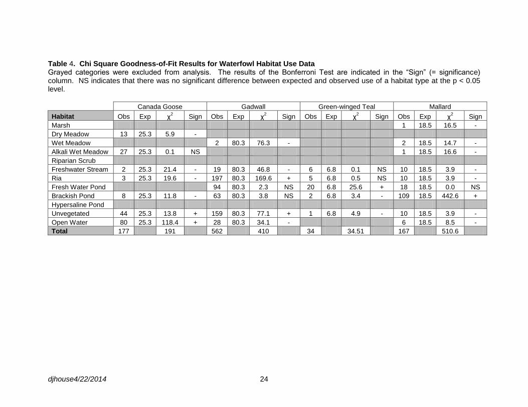
djhouse4/22/2014 24

Table 4. Chi Square Goodness-of-Fit Results for Waterfowl Habitat Use Data Grayed categories were excluded from analysis. The results of the Bonferroni Test are indicated in the “Sign” (= significance) column. NS indicates that there was no significant difference between expected and observed use of a habitat type at the p < 0.05 level.

Canada Goose Gadwall Green-winged Teal Mallard

Habitat Obs Exp χ2 Sign Obs Exp χ

2 Sign Obs Exp χ

2 Sign Obs Exp χ

2 Sign

Marsh 1 18.5 16.5 -

Dry Meadow 13 25.3 5.9 -

Wet Meadow 2 80.3 76.3 - 2 18.5 14.7 -

Alkali Wet Meadow 27 25.3 0.1 NS 1 18.5 16.6 -

Riparian Scrub

Freshwater Stream 2 25.3 21.4 - 19 80.3 46.8 - 6 6.8 0.1 NS 10 18.5 3.9 -

Ria 3 25.3 19.6 - 197 80.3 169.6 + 5 6.8 0.5 NS 10 18.5 3.9 -

Fresh Water Pond 94 80.3 2.3 NS 20 6.8 25.6 + 18 18.5 0.0 NS

Brackish Pond 8 25.3 11.8 - 63 80.3 3.8 NS 2 6.8 3.4 - 109 18.5 442.6 +

Hypersaline Pond

Unvegetated 44 25.3 13.8 + 159 80.3 77.1 + 1 6.8 4.9 - 10 18.5 3.9 -

Open Water 80 25.3 118.4 + 28 80.3 34.1 - 6 18.5 8.5 -

Total 177 191 562 410 34 34.51 167 510.6

djhouse4/22/2014 25

Table 5. Summary of 2013 Mono Lake Fall Aerial Survey Count Data

Species 3-Sep 19-Sep 1-Oct 15-Oct 29-Oct 12-Nov Total

detections %

Total

Snow Goose 13 13 0.1%

Cackling Goose 5 4 9 <0.1%

Canada Goose 65 45 33 36 179 0.8%

Gadwall 105 51 68 21 3 15 263 1.1%

Mallard 19 40 35 47 8 97 246 1.0%

Blue-winged Teal 2 2 <0.1%

Cinnamon Teal 25 25 0.1%

Northern Shoveler 6008 7860 1633 2227 43 17771 74.9%

Northern Pintail 1316 13 10 1339 5.6%

Green-winged Teal 13 12 55 190 36 120 426 1.8%

Unidentified Teal 1 320 5 1 327 1.4%

Redhead 1 1 <0.1%

Lesser Scaup 1 1 <0.1%

Bufflehead 3 3 <0.1%

Ruddy Duck 62 225 607 1210 538 465 3107 13.1%

Total Waterfowl 6207 8213 3782 4065 692 753 23712

Species Richness 5 6 9 7 8 10

Table 6. 2013 Fall Spatial Distribution of Waterfowl at Mono Lake

Lakeshore Segment 3-Sep 19-Sep 1-Oct 15-Oct 29-Oct 12-Nov

Segment Total

% by Segment

BLPO 4 2 5 9 20 0.1%

BRCR 16 16 0.1%

DECR 207 510 688 1475 11 4 2895 13.6%

DEEM 31 72 233 8 344 1.6%

LVCR 31 19 31 15 5 8 109 0.5%

MICR 1550 1802 530 445 10 4337 20.4%

NESH 0 0.0%

RACO 4 13 1 8 26 0.1%

RUCR 5 65 63 16 11 160 0.8%

SASP 258 1105 249 87 36 24 1759 8.3%

SOTU 8 7 86 3 104 0.5%

SSLA 280 440 102 6 30 858 4.0%

WASP 20 30 12 10 35 160 267 1.3%

WESH 305 125 76 28 534 2.5%

WICR 3800 4000 1200 858 9858 46.3%

Lakewide total 6190 7980 3441 3085 272 319 21287

djhouse4/22/2014 26

Table 7. Summary of 2013 Bridgeport Reservoir Fall Aerial Survey Count Data


detections % Total

Canada Goose 45 55 550 250 190 1090 5.8%

Tundra Swan 5 5 <0.1%

Gadwall 1425 440 75 139 80 110 2269 12.2%

American Wigeon 15 8 23 0.1%

Mallard 600 7 102 252 168 540 1669 8.9%

Cinnamon Teal 50 50 0.3%

Northern Shoveler 4375 1802 150 6327 33.9%

Northern Pintail 106 800 330 24 8 1268 6.8%


Unidentified Teal 200 940 37 75 1252 6.7%

Canvasback 10 10 0.1%

Ring-necked Duck 10 10 0.1%

Lesser Scaup 25 25 0.1%

Bufflehead 30 56 86 0.5%

Common Merganser 33 17 10 60 0.3%

Ruddy Duck 556 760 405 124 1118 2963 15.9%

Total Waterfowl 7430 4108 2616 1439 826 2237 18656


Table 8. 2013 Fall Spatial Distribution of Waterfowl at Bridgeport Reservoir

Lakeshore Segment 3-Sep 19-Sep 1-Oct 15-Oct 29-Oct 12-Nov

Segment Total

% by Segment

EASH 1203 51 300 141 38 34 1767 9.5%

NOAR 137 74 51 15 98 13 388 2.1%

WEBA 6090 3983 2265 1283 690 2190 16501 88.4%

Lakewide total 7430 4108 2616 1439 826 2237 18656

djhouse4/22/2014 27

Table 9. Summary of 2013 Crowley Reservoir Fall Aerial Survey Count Data


detections %

Total

Greater White-fronted Goose 4 1 5 <0.1%

Ross's Goose 1 1 <0.1%

Cackling Goose 1 1 <0.1%

Canada Goose 90 172 42 80 384 0.6%

Tundra Swan 7 7 <0.1%

Gadwall 776 1237 1877 818 1052 667 6427 10.3%

American Wigeon 2 17 15 35 40 288 397 0.6%

Mallard 850 525 1820 3138 2519 2426 11278 18.1%

Blue-winged Teal 5 5 <0.1%

Cinnamon Teal 55 21 76 0.1%

Northern Shoveler 1947 5166 3425 1885 510 15 12948 20.8%

Northern Pintail 125 607 1642 1634 3393 843 8244 13.2%


Unidentified Teal 30 2 32 0.1%

Canvasback 3 3 <0.1%

Redhead 58 4 4 10 76 0.1%

Ring-necked Duck 35 6 34 20 95 0.2%

Lesser Scaup 14 127 141 0.2%

Bufflehead 2 1 18 127 265 413 0.7%

Hooded Merganser 4 4 <0.1%

Common Merganser 5 5 <0.1%

Ruddy Duck 367 579 1353 6524 3967 2400 15190 24.4%

Total Waterfowl 5269 9524 11160 16089 12270 8050 62362


Table 10. 2013 Fall Spatial Distribution of Waterfowl at Crowley Reservoir

Lakeshore Segment 3-Sep 19-Sep 1-Oct 15-Oct 29-Oct 12-Nov Segment

Total % by

Segment

CHCL 15 130 189 437 551 1322 2.1%

HIBA 144 227 375 540 82 334 1702 2.7%

LASP 102 341 257 366 703 1447 3216 5.2%

MCBA 3098 6972 6581 12276 9051 4107 42085 67.5%

NOLA 35 160 247 521 189 1152 1.8%

SAPO 37 9 80 231 80 429 866 1.4%

UPOW 1888 1925 3577 2240 1396 993 12019 19.3%

Lakewide total 5269 9524 11160 16089 12270 8050 62362

djhouse4/22/2014 28

Table 11. Mono Lake Restoration Ponds - Total Summer Detections

Species COPOE COPOW DEPO_1 DEPO_2 DEPO_3 DEPO_4 DEPO_5 Total

Cinnamon Teal 1 1

Gadwall 21 2 23


Mallard 2 2

Ruddy Duck 5 7 4 16

Pond Totals 32 0 0 1 7 6 0 46

Table 12. Mono Lake Restoration Ponds - Total Waterfowl Broods

Species County Ponds DeChambeau Ponds

Gadwall 4 1

Green-winged Teal 1

Ruddy Duck 1

Total Broods 4 3

Table 13. Mono Lake Restoration Ponds - 2013 Fall Survey Counts

County Ponds 3-Sep 19-Sep 1-Oct 15-Oct 29-Oct 12-Nov Total Fall

Detections

Tundra Swan 1 1

Gadwall 4 4

Mallard 3 2 1 6

Unidentified Teal 10 12 20 42

Ring-necked Duck 3 3

Total Waterfowl 24 12 3 20 4 3 66

DeChambeau Ponds 3-Sep 19-Sep 1-Oct 15-Oct 29-Oct 12-Nov Total Fall

Detections

Mallard 3 1 5 9

Gadwall 4 5 5 14

Unidentified Teal 3 6 5 14

Bufflehead 1 1

Total Waterfowl 10 6 6 10 5 1 38

djhouse4/22/2014 29

Figure 1. Summer Ground Count Survey Areas

LVCR

RUCR

DECR

MICR WICR

DEPO

COPO

SOTU

SSLA

SASP

WASP

djhouse4/22/2014 30

Figure 2. Mono Lake Fall Aerial Survey Lakeshore Segments, Boundaries, and Cross-Lake Transects

3a 3b 3c 3d

4a 4b 4c 4d

5a 5b 5c 5d

6a 6b 6c

7a 7b 7c

8a 8b

BRCR

DEEM

MICR BLPO

WICR

DECR

WESH

LVCR

RACO

RUCR

NESH

WASP

SASP

SSLA

SOTU

1a 1b

2a 2b 2c

djhouse4/22/2014 31

Figure 3. Bridgeport Reservoir Lakeshore Segments and Segment Boundaries

North Arm

West Bay

East Shore

djhouse4/22/2014 32

Figure 4. Crowley Reservoir Lakeshore Segments and Segment Boundaries

UPOW

SAPO

NOLA

MCBA

HIBA

CHCL

LASP

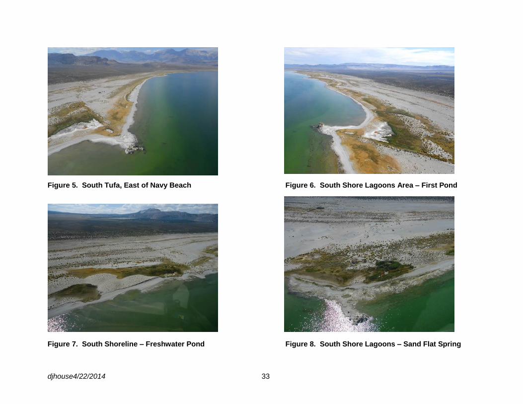
djhouse4/22/2014 33

Figure 5. South Tufa, East of Navy Beach Figure 6. South Shore Lagoons Area – First Pond

Figure 7. South Shoreline – Freshwater Pond Figure 8. South Shore Lagoons – Sand Flat Spring

djhouse4/22/2014 34

Figure 9. South Shore Lagoons Goose Springs Outflow Area Figure 10. Sammann’s Spring West of Tufa Grove

Figure 11. Sammann’s Spring, east of Tufa grove Figure 12. Warm Springs – North Pond

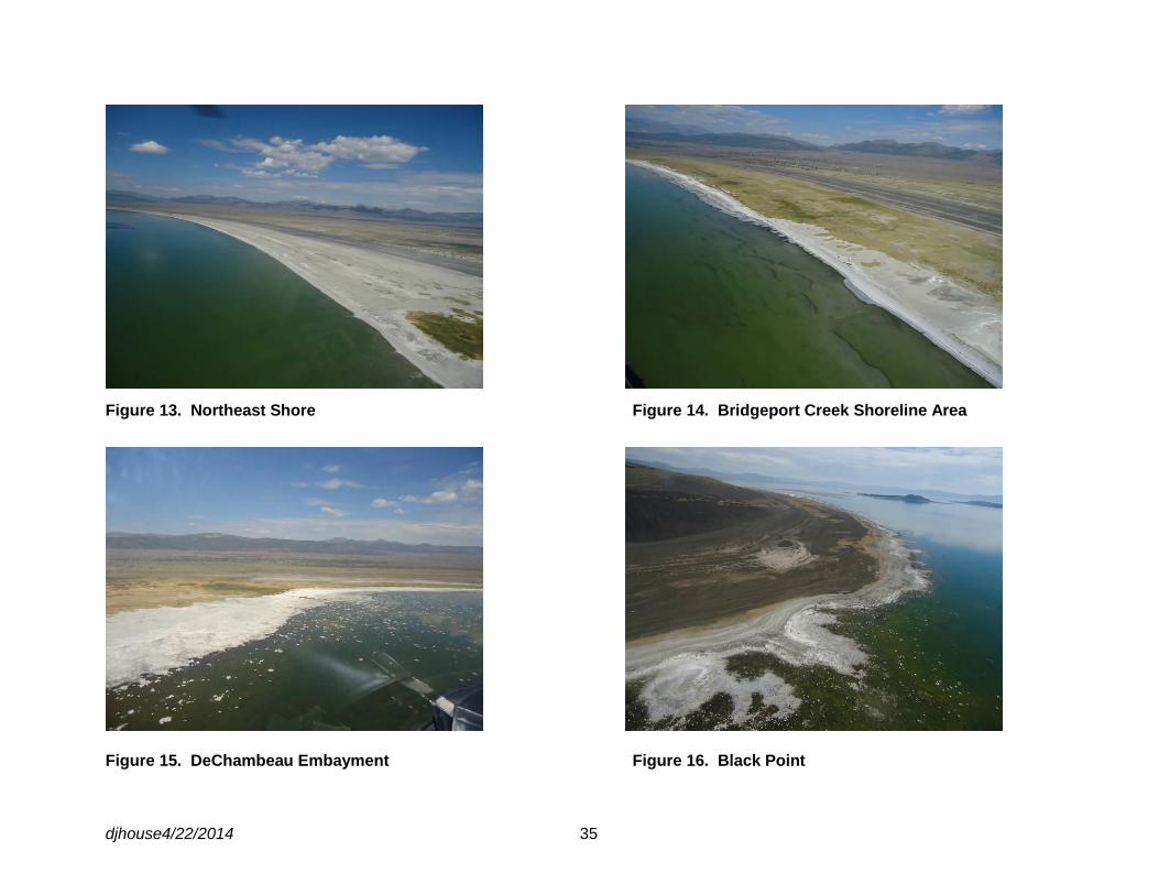
djhouse4/22/2014 35

Figure 13. Northeast Shore Figure 14. Bridgeport Creek Shoreline Area

Figure 15. DeChambeau Embayment Figure 16. Black Point

djhouse4/22/2014 36

Figure 17. Wilson Creek Shoreline Area Figure 18. Mill Creek Delta

Figure 19. DeChambeau Creek Shoreline Area

djhouse4/22/2014 37

Figure 20. West Shore Figure 21. Lee Vining Creek Delta

Figure 22. Ranch Cove Shoreline Area Figure 23. Rush Creek Delta

Sammann’s Spring 330789E, 4206026N 331011E, 4206341N

South Shore Lagoons 328120E, 4203811N 328552E, 4204084N

djhouse4/22/2014 38

Figure 24. Photo of Bridgeport Reservoir, Looking North Photo shows the West Bay area and the south end of the East Shore area. The majority of waterfowl that use Bridgeport Reservoir in the fall congregate in this southern end of the reservoir.

East Shore

North Arm

West Bay

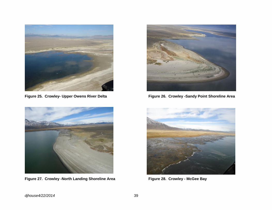
djhouse4/22/2014 39

Figure 25. Crowley- Upper Owens River Delta Figure 26. Crowley -Sandy Point Shoreline Area

Figure 27. Crowley -North Landing Shoreline Area Figure 28. Crowley - McGee Bay

djhouse4/22/2014 40

Figure 29. Crowley -Hilton Bay Figure 30. Crowley - Chalk Cliffs

Figure 31. Crowley - Layton Springs

djhouse4/22/2014 41

Figure 32. 2013 Brood Locations The number in parentheses indicates the number of broods found in each area.

Rush Creek (5)

Lee Vining Creek (0)

DeChambeau Creek (2)

Mill (3) and Wilson (10) Creeks

RestorationPonds (7)

South Shore Lagoons (6)

Sammann’s Spring (3)

South Tufa (3)

djhouse4/22/2014 42

Figure 33. Waterfowl Habitat Use The numbers in parentheses indicate sample size. The bars represent the percent of the total observations.

(562)

(34)

(167)

(177)

djhouse4/22/2014 43

Figure 34. Total Fall Detections by Waterbody

djhouse4/22/2014 44

Figure 35. Relationship Between Total Waterfowl and Lake Elevation in June

Figure 36. Number of Waterfowl Broods versus Lake Elevation in June

r=0.920 p<0.01

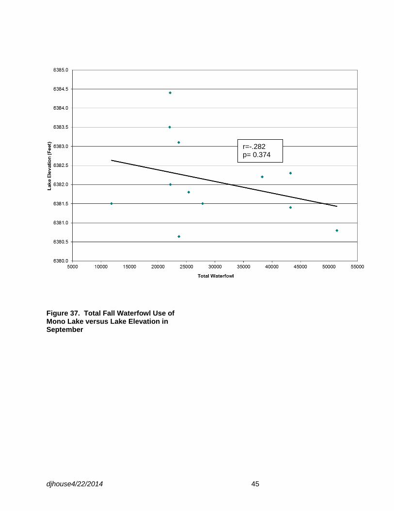
djhouse4/22/2014 45

Figure 37. Total Fall Waterfowl Use of Mono Lake versus Lake Elevation in September

r=-.282 p= 0.374

djhouse4/22/2014 46

APPENDICES Appendix 1. 2013 Ground Count Survey Dates and Times

Survey 3

Survey 1

Survey 2

3-Jun 4-Jun 5-Jun 6-Jun

RUCR 1223 - 1350 hrs

SOTU 0915-1053 hrs

SSLA 1141 - 1442 hrs 0610 - 0903 hrs

DECR 0545 - 0700 hrs

MICR 0700 - 0813 hrs

WICR 0815 - 0900 hrs

LVCR 1035 - 1135 hrs

DEPO 1300-1400 hrs

COPO 1300-1400 hrs

SASP 1108 - 1445 hrs

WASP 0715 - 1108 hrs

Survey

Area

Survey Date and Time

24-Jun 25-Jun 26-Jun 27-Jun

RUCR 0538 - 0702 hrs

SOTU 0537 - 0616 hrs

SSLA 0807 - 1020 hrs

DECR 0550 - 0640 hrs

MICR 0640 - 0738 hrs

WICR 0730 - 0825 hrs

LVCR 1107 - 1155 hrs

DEPO 1000 - 1032 hrs

COPO 1000 - 1032 hrs

SASP 0600 - 0845 hrs

WASP 0828 - 1000 hrs

Survey

Area


15-Jul 16-Jul 17-Jul 18-Jul

RUCR 0540 - 0645 hrs

SOTU 0550 - 0645 hrs

SSLA 0751 - 1010 hrs

DECR 0555 - 0645 hrs

MICR 0645 - 0728 hrs

WICR 0728 - 0810 hrs

LVCR 1445 - 1515 hrs

DEPO 1339 - 1425 hrs

COPO 1339 - 1425 hrs

SASP 0655 - 0942 hrs

WASP 0850 - 1023 hrs

Survey

Area


djhouse4/22/2014 47

Appendix 2. Common and Scientific Names for Species Referenced in the Document.

Common Name Scientific Name

Greater White-fronted Goose Anser albifrons

Snow Goose Chen caerulescens

Ross's Goose Chen rossii

Cackling Goose Branta hutchinsii

Canada Goose Branta canadensis

Tundra Swan Cygnus columbianus

Gadwall Anas strepera

American Wigeon Anas americana

Mallard Anas platyrhynchos

Blue-winged Teal Anas discors

Cinnamon Teal Anas cyanoptera

Northern Shoveler Anas clypeata

Northern Pintail Anas acuta

Green-winged Teal Anas crecca

Unidentified Teal Anas (sp)

Canvasback Aythya valisineria

Redhead Aythya americana

Ring-necked Duck Aythya collaris

Lesser Scaup Aythya affinis

Bufflehead Bucephala albeola

Hooded Merganser Lophodytes cucullatus

Common Merganser Mergus merganser

Ruddy Duck Oxyura jamaicensis

djhouse4/22/2014 48

Appendix 3. Habitat Categories Used for Documenting Use by Waterfowl Species (from 1999 Mono Basin Habitat and Vegetation Mapping, Los Angeles Department of Water and Power 2000).

Marsh

Areas with surface water usually present all year and dominated by tall emergent species such as hard-stem bulrush (Scirpus acutus), cattail (Typhus latifolia), three-square (Scirpus pungens), alkali bulrush (Scirpus maritimus) and beaked sedge (Carex utriculata).

Wet Meadow Vegetation with seasonally or permanently wet ground dominated by lower stature herbaceous plant species, such as sedges (Carex spp.), rushes (Juncus spp.), spikerushes (Eleocharis spp.), and some forbs (e.g. monkey flower [Mimulus spp.], paintbrush [Castilleja exilis]). Wet meadow vegetation was in areas where alkaline or saline soils did not appear to be present. This class included the “mixed marsh” series from Jones and Stokes 1993 mapping.

Alkaline Wet Meadow This type was similar in stature to the wet meadow class but occurred in areas clearly affected by saline or alkaline soils. Vegetation was typically dominated by dense stands of Nevada bulrush (Scirpus nevadensis), Baltic rush (Juncus balticus), and/or saltgrass (Distichlis spicata). The high density and lushness of the vegetation indicated that it had a relatively high water table with at least seasonal inundation and distinguished it from the dry meadow vegetation class.

Dry meadow/forb This vegetation class included moderately dense to sparse (at least 15 percent) cover of herbaceous species, including a variety of grasses and forbs and some sedges (e.g. Carex douglasii). As with the alkaline wet meadow type above, comparison to vegetation series in Jones and Stokes (1993) was sometimes problematic due to difficulty in distinguishing dry meadow from wet meadow types.

Riparian and wetland scrub Areas dominated by willows (Salix spp.) comprised most of the vegetation classified as riparian.wetlands scrub. Small amounts of buffalo berry (Shepardia argentea) and Wood’s rose (Rosa woodsii) usually mixed with willow also were included in this class.

Great Basin scrub Scattered to dense stands of sagebrush (Artemisia tridentata), rabbitbrush (Chrysothamnus nauseosus), and/or bitterbrush (Purshia tridentata) were classified as Great Basin scrub. This vegetation type included a range of soil moisture conditions, as rabbitbrush was often found in moist areas close to the lakeshore and sagebrush was typically in arid upland areas.

djhouse4/22/2014 49

Riparian forest and woodland Aspen (Populus tremuloides) and black cottonwood (Populus trichocarpa) were the two tree species most common in the riparian forest/woodland vegetation type.

Freshwater-stream Freshwater-stream habitats are watered; freshwater channels such as exist in Rush Creek and Lee Vining Creeks.

Freshwater-ria Freshwater-ria areas were surface water areas at the mouths of streams that likely have some salt/freshwater stratification.

Freshwater-pond This type included ponds fed by springs within marsh areas or artificially by diversions from streams (e.g. DeChambeau/County ponds).

Ephemeral Brackish Pond Ponds along the shoreline created by the formation of littoral bars with an extensive area of marsh or wet meadow indicating the presence of springs was present landward, were identified as ephemeral brackish ponds. In some cases, ponds were not completely cut off from lake water, but were judged to still have brackish water due to freshwater input and reduced mixing.

Ephemeral Hypersaline Pond Ponds along the shoreline created by the formation of littoral bars, but without an extensive area of marsh or wet meadow present landward, were identified as ephemeral hypersaline ponds. These were presumed to contain concentrated brine due to evaporation.

Unvegetated Unvegetated areas were defined as those that were barren to sparsely vegetated (<15 percent cover). This class included sandy areas, alkaline flats, tufa, and delta outwash deposits.

djhouse4/22/2014 50

Appendix 4. 2013 Fall Aerial Survey Dates

Survey Number 1 2 3 4 5 6

Mono Lake 3-Sep 19-Sep 1-Oct 15-Oct 29-Oct 12-Nov

Bridgeport Reservoir 3-Sep 19-Sep 1-Oct 15-Oct 29-Oct 12-Nov

Crowley Reservoir 3-Sep 19-Sep 1-Oct 15-Oct 29-Oct 12-Nov

Appendix 5. Lakeshore Segment Boundaries (UTM, Zone 11, NAD 27, CONUS)

Mono Lake Lakeshore Segment Code Easting Northing

South Tufa SOTU 321920 4201319

South Shore Lagoons SSLA 324499 4201644

Sammann’s Spring SASP 328636 4204167

Warm Springs WASP 332313 4208498

Northeast Shore NESH 330338 4213051

Bridgeport Creek BRCR 324773 4215794

DeChambeau Embayment DEEM 321956 4214761

Black Point BLPT 318252 4211772

Wilson Creek WICR 315680 4209358

Mill Creek MICR 313873 4209544

DeChambeau Creek DECR 312681 4209246

West Shore WESH 315547 4208581

Lee Vining Creek LVCR 314901 4205535

Ranch Cove RACO 316077 4204337

Rush Creek RUCR 318664 4202603

Crowley Reservoir

Upper Owens UPOW 346150 4168245

Sandy Point SAPO 345916 4167064

North Landing NOLA 346911 4164577

McGee Bay MCBA 345016 4164414

Hilton Bay HIBA 346580 4161189

Chalk Cliff CHCL 347632 4162545

Layton Springs LASP 347177 4165868

Bridgeport Reservoir

North Arm NOAR 306400 4244150

West Bay WEBA 304100 4240600

East Shore EASH 305600 4237600

djhouse4/22/2014 51

Appendix 6. Mono Lake Cross-Lake Transect Positions

Cross-Lake Transect Number Latitude

1 37º 57’00”

2 37º 58’00”

3 37º 59’00”

4 38º 00’00”

5 38º 01’00”

6 38º 02’00”

7 38º 03’00”

8 38º 04’00”

Documents

Section 4 Mono Basin Waterfowl Habitat and Population ... and Population Monitoring . RY 2013-14 . APPENDIX 1 ... The limnological monitoring program consists of four components: