Section 3 - LogintoLearn - your gateway to learning in … 3 Topics Covered" Calculating using formulas..... 3-2 " Copying formulas..... 3-7 " Using absolute cell addresses ..... 3-13

Microsoft Excel 2000 Introductory Course ! Student Workbook ! © 2000 ! www.StudyIT.net 3-1

Section 3

Topics Covered " Calculating using formulas .............................................. 3-2 " Copying formulas............................................................. 3-7 " Using absolute cell addresses ........................................ 3-13 " Calculating results using AutoCalculate........................ 3-18#" Using functions .............................................................. 3-21 " Working with dates and times ....................................... 3-28

Time Required: 2 Hr 20 Mins


Calculating Using Formulas

When you want to specify a calculation that is to be performed by Excel, you do so by entering a formula into the cell. Excel will then carry out the calculation and display the result in the cell containing the formula. The formula itself can be seen, in the formula bar, only when the active cell pointer is on the cell.

When entering a formula into a cell, you must begin by typing an = equals sign so that Excel recognises the entry as a formula. The formula can then be entered using any of the standard operators shown below.

Operators * Multiply / Divide + Add - Subtract % Percent ^ Exponent (to the power of)

Example Formula =6+7+2 If this formula is entered into a cell, the result (15) will be displayed in the

cell. The formula will be displayed only in the formula bar when the active cell pointer is on the cell.

Formula Construction Although formulas can be constructed using actual values as in the example above, you should replace actual values with cell references wherever possible. When cell references are used, the result of the formula will be automatically updated if the contents of the cell change, making the formula dynamic.

For example, if the formula =B6*20% is entered into a cell, the cell will display the result 20 if cell B6 contains 100, but it will be automatically updated if another value is entered into cell B6.

To ensure that the calculations in a formula are carried out in the correct order, you can use parenthesis (brackets) to identify those calculations that should be performed first. For example, in the formula =(B5+C5+D5)*2.5%, the cells B5, C5 and D5 will be added before the result is multiplied by 2.5%.

HelpTip: To see the result of your formula as you build it, click the Edit Formula button shown on the formula bar to display the formula palette.



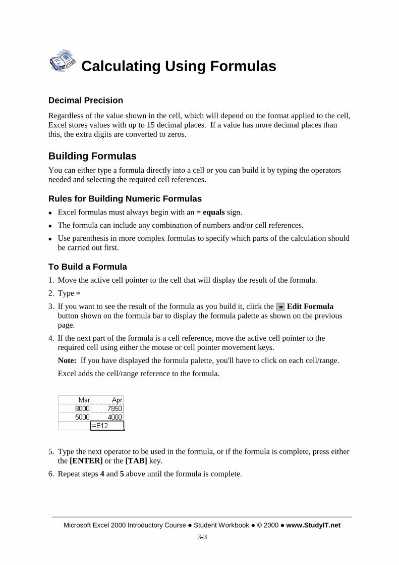
Decimal Precision Regardless of the value shown in the cell, which will depend on the format applied to the cell, Excel stores values with up to 15 decimal places. If a value has more decimal places than this, the extra digits are converted to zeros.

Building Formulas You can either type a formula directly into a cell or you can build it by typing the operators needed and selecting the required cell references.

Rules for Building Numeric Formulas ! Excel formulas must always begin with an = equals sign. ! The formula can include any combination of numbers and/or cell references. ! Use parenthesis in more complex formulas to specify which parts of the calculation should

be carried out first.

To Build a Formula 1. Move the active cell pointer to the cell that will display the result of the formula. 2. Type = 3. If you want to see the result of the formula as you build it, click the Edit Formula

button shown on the formula bar to display the formula palette as shown on the previous page.

4. If the next part of the formula is a cell reference, move the active cell pointer to the required cell using either the mouse or cell pointer movement keys.

Note: If you have displayed the formula palette, you'll have to click on each cell/range. Excel adds the cell/range reference to the formula.

5. Type the next operator to be used in the formula, or if the formula is complete, press either

the [ENTER] or the [TAB] key. 6. Repeat steps 4 and 5 above until the formula is complete.



Circular References If a formula contains a reference to its own cell, either directly or indirectly, it creates what's called a circular reference. For example, if you enter =B6*B7 into cell B7, you will have created a circular reference. The status bar will display a message telling you there's a circular reference and which cell it's in, and depending on the method you've used to create the formula, this dialogue box may be displayed.

Note: If the Office Assistant is switched on, this message will look different but will contain the same information.

To resolve the problem, edit the formula to remove the circular reference.


Exercise 3-1 1. Using the File, Open command, open the workbook Price stored in the Excel 2000 Intro

Exercises folder.

2. Follow the instructions below to enter a formula that will calculate the Profit for each product. — Move the active cell pointer to cell C7, the cell where the result is to be shown. The Profit is calculated by multiplying the Production Costs by 15%. — Click the Edit Formula button. — Click on cell B7 to add this cell to the formula. Notice the result of the formula so far which is displayed in the formula palette.

— Type *15% then press [ENTER] or click OK to enter the formula into the cell. The result (265.70) is displayed in cell C7.


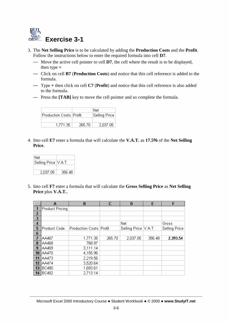
Exercise 3-1 3. The Net Selling Price is to be calculated by adding the Production Costs and the Profit.

Follow the instructions below to enter the required formula into cell D7. — Move the active cell pointer to cell D7, the cell where the result is to be displayed,

then type = — Click on cell B7 (Production Costs) and notice that this cell reference is added to the

formula. — Type + then click on cell C7 (Profit) and notice that this cell reference is also added

to the formula. — Press the [TAB] key to move the cell pointer and so complete the formula.

4. Into cell E7 enter a formula that will calculate the V.A.T. as 17.5% of the Net Selling Price.

5. Into cell F7 enter a formula that will calculate the Gross Selling Price as Net Selling Price plus V.A.T..


Copying Formulas

As you have seen, there are a number of commands that can be used to copy data from one location in the workbook to another. The same commands can be used to copy cells containing formulas. Which command you should use will depend on where the copied data is to appear.

Copying a Formula to Contiguous Cells The easiest way to copy a formula to contiguous cells, cells that border the cell containing the formula, is to use the AutoFill handle. However, you could also use one of the options from the Edit, Fill cascading menu: select the cell containing the formula and the cell(s) into which it is to be copied, select the Edit, Fill command to display the cascading menu and choose the appropriate option; Up, Down, Left or Right.

Copying a Formula to Non-contiguous Cells If the cell(s) into which the formula is to be copied is non-contiguous, cells that do not border the cell containing the formula, you could use the Copy and Paste options from the Edit menu, or you could use drag-and-drop. If, however, the formula is to be copied to another workbook or another application then you should use the Copy and Paste options.

Relative Cell Addresses When a formula is copied, the cell references in the formula are updated to reflect the formula's new location on the worksheet.

For example, if you enter the formula =B3+C3 into cell D3 as shown below,

and then copy the formula to cell D4, the formula in D4 will be changed to =B4+C4

For this reason, the cell references in this formula are called relative cell addresses.


Exercise 3-1 6. Copy the formula down column C by clicking and dragging the AutoFill handle down to

cell C14. Click on cell C8 and notice that the formula, shown in the formula bar, has been updated to make reference to row 8.

7. Copy the formula by selecting the range D7:D14 and then selecting the Edit, Fill, Down command.

8. Copy the formula in cell E7 down the column using drag-and-drop. Notice that you can copy to only one cell at a time using drag-and-drop. Use one of the other copying methods to complete column E.

9. Follow the instructions below to copy the formula in cell F7 to the range F8:F14. — Click on cell F7 then select the Edit, Copy command. — Select the range F8:F14 then press the [ENTER] key to insert the copied formula into

each cell in the range.


Exercise 3-1 10. Follow the instructions below to insert 2 new rows below product AA470.

— Select rows 11 and 12 by clicking and dragging over their row heading buttons. — Move the mouse pointer onto the selection then click the right mouse button to

display the shortcut menu and choose Insert.

11. Enter the details shown below into the inserted rows.

12. As product BC480 is no longer being produced, delete its row by clicking on row 15 heading button and then selecting the Edit, Delete command.

13. Format the worksheet as shown below using the options available from the Formatting toolbar. Use the Fill Color button to apply the grey shading.

14. Save the changes to the worksheet then close it.


Exercise 3-2 1. For some additional practice, open the file called Dealer Pricing and enter formulae on

this worksheet to complete it as shown below.

2. Save the changes and close the worksheet.


Exercise 3-3 1. Open the file called Cash Flow Projections held in the Excel 2000 Intro Exercises

folder. 2. Complete the totals on rows 8 and 19 and column H. 3. In B22 calculate the closing bank balance taking into account the opening bank

balance, total income and total expenditure. 4. Create formulae for February's open and closing balances that can be copied across

each column to show the opening and closing bank balance for each month.

5. Save and close the workbook.


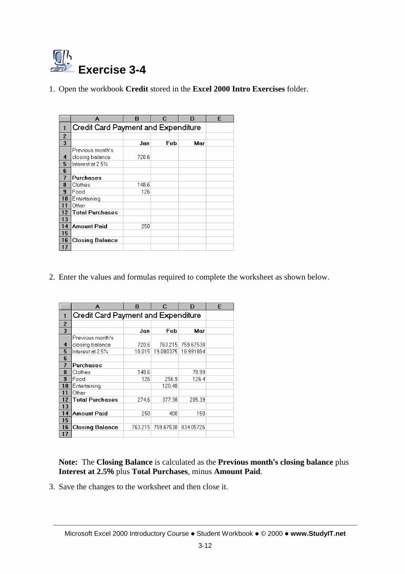
Exercise 3-4 1. Open the workbook Credit stored in the Excel 2000 Intro Exercises folder.

2. Enter the values and formulas required to complete the worksheet as shown below.

Note: The Closing Balance is calculated as the Previous month's closing balance plus

Interest at 2.5% plus Total Purchases, minus Amount Paid.

3. Save the changes to the worksheet and then close it.


Absolute Cell Addresses

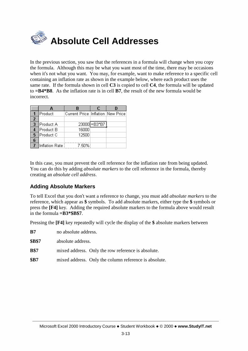
In the previous section, you saw that the references in a formula will change when you copy the formula. Although this may be what you want most of the time, there may be occasions when it's not what you want. You may, for example, want to make reference to a specific cell containing an inflation rate as shown in the example below, where each product uses the same rate. If the formula shown in cell C3 is copied to cell C4, the formula will be updated to =B4*B8. As the inflation rate is in cell B7, the result of the new formula would be incorrect.

In this case, you must prevent the cell reference for the inflation rate from being updated. You can do this by adding absolute markers to the cell reference in the formula, thereby creating an absolute cell address.

Adding Absolute Markers To tell Excel that you don't want a reference to change, you must add absolute markers to the reference, which appear as $ symbols. To add absolute markers, either type the $ symbols or press the [F4] key. Adding the required absolute markers to the formula above would result in the formula =B3*$B$7.

Pressing the [F4] key repeatedly will cycle the display of the $ absolute markers between

B7 no absolute address.

$B$7 absolute address.

B$7 mixed address. Only the row reference is absolute.

$B7 mixed address. Only the column reference is absolute.


Exercise 3-5 1. Open the workbook Salrise stored in the Excel 2000 Intro Exercises folder.

2. Enter a formula into cell C6 that will calculate the Annual Salary of Paul Hull then copy the formula for the other employees.

3. Cell B3 contains the percentage rise that the employees are to be given. Follow the instructions below to enter a formula that will calculate the Increase for Paul Hull into cell D6 and then copy it for the other employees. — Position the active cell pointer on cell D6 then type =C6*B3 As this calculation requires a specific reference to cell B3, the formula must include

an absolute cell address. Otherwise, the reference to cell B3 would be changed, giving an incorrect result.

— Change the reference to cell B3 in the formula to read $B$3. You can add the $ signs either by typing them, or by positioning the insertion point on the B3 reference and then pressing [F4].

— Press the [TAB] key to complete the formula. — Click on cell D6 then use the AutoFill handle to copy this formula for the other

employees. — Click on cell D10 and look at the formula in the formula bar. The reference to cell C6

has been changed to reflect the formula's location on the worksheet, but the reference to cell B3 remains the same.


Exercise 3-5 4. Enter a formula into cell E6 that will calculate Paul Hull's New Salary (Annual Salary +

Increase) then copy it for the other employees. 5. Calculate the totals on row 11 for each of the columns.

6. Notice the total Increase shown in cell D11. The management have budgeted to spend a

maximum of 6,200 on salary increases and, as you can see, awarding a 5% increase will exceed the budget. As the increase percentage is being taken from cell B3, type other values, such as 3.5% and 4.25%, into cell B3, to find the highest percentage that management could award without exceeding its budget.

7. Save the changes to the workbook and then close it.


Exercise 3-6 1. Open the file called Time Sheet held in the Excel 2000 Intro Exercises folder. 2. Complete the worksheet as shown below, by calculating how much each person is due

based on the hours they worked and the pay rates show in the cell range A16:B18.



Exercise 3-7 1. Open the file called Travelling Speed. Following the idea that Speed = Distance

divided by Time, in this exercise, you will enter a single formula in cell B3 that can be copied to complete the sheet

2. Enter the following formula into B3: =B$2/$A3 This formula instructs Excel not to

change the row reference 2 and the column reference A when copied (as they are preceded by absolute markers $)

3. Copy this formula down column B and then copy the formulae in column B across to

column K to complete the sheet as shown below.

4. Save and close the file.

Microsoft Excel 2000 Introductory Course !

Calculating Results Using AutoCalculate

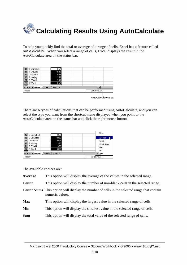
To help you quickly find the total or average of a range of cells, Excel has a feature called AutoCalculate. When you select a range of cells, Excel displays the result in the AutoCalculate area on the status bar.

There are 6 types of calculations that can beselect the type you want from the shortcut mAutoCalculate area on the status bar and clic

The available choices are:

Average This option will display the a

Count This option will display the n

Count Nums This option will display the nnumeric values.

Max This option will display the l

Min This option will display the s

Sum This option will display the to
AutoCalculate area
Student Workbook ! © 2000 ! www.StudyIT.net 3-18

performed using AutoCalculate, and you can enu displayed when you point to the k the right mouse button.

verage of the values in the selected range.

umber of non-blank cells in the selected range.

umber of cells in the selected range that contain

argest value in the selected range of cells.

mallest value in the selected range of cells.

tal value of the selected range of cells.


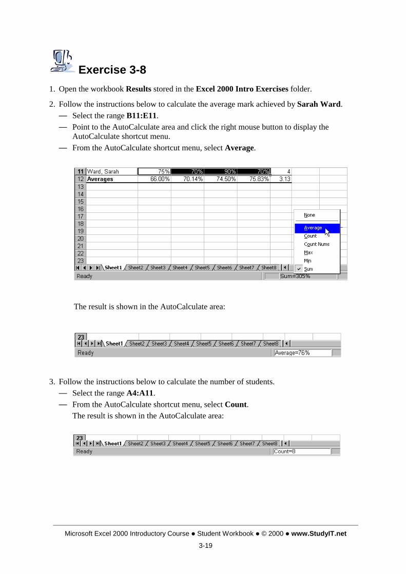
Exercise 3-8 1. Open the workbook Results stored in the Excel 2000 Intro Exercises folder.

2. Follow the instructions below to calculate the average mark achieved by Sarah Ward. — Select the range B11:E11. — Point to the AutoCalculate area and click the right mouse button to display the

AutoCalculate shortcut menu. — From the AutoCalculate shortcut menu, select Average.

The result is shown in the AutoCalculate area:

3. Follow the instructions below to calculate the number of students.

— Select the range A4:A11. — From the AutoCalculate shortcut menu, select Count. The result is shown in the AutoCalculate area:


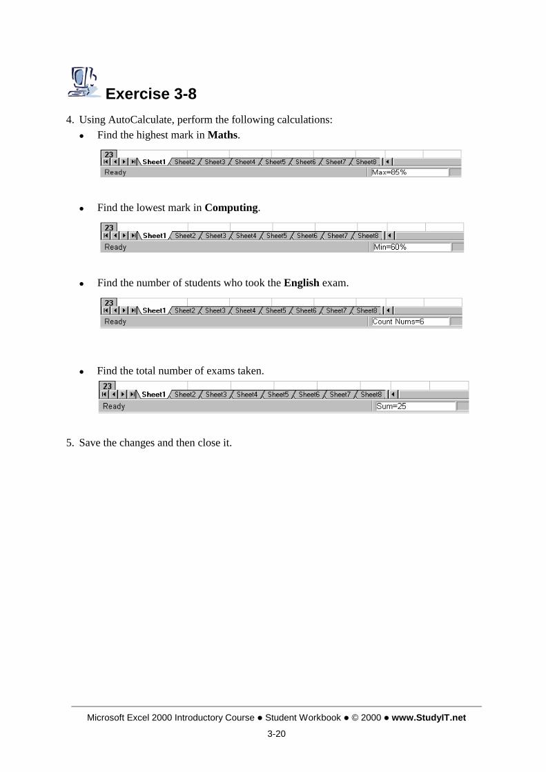
Exercise 3-8 4. Using AutoCalculate, perform the following calculations:

! Find the highest mark in Maths.

! Find the lowest mark in Computing.

! Find the number of students who took the English exam.

!# Find the total number of exams taken.

5. Save the changes and then close it.


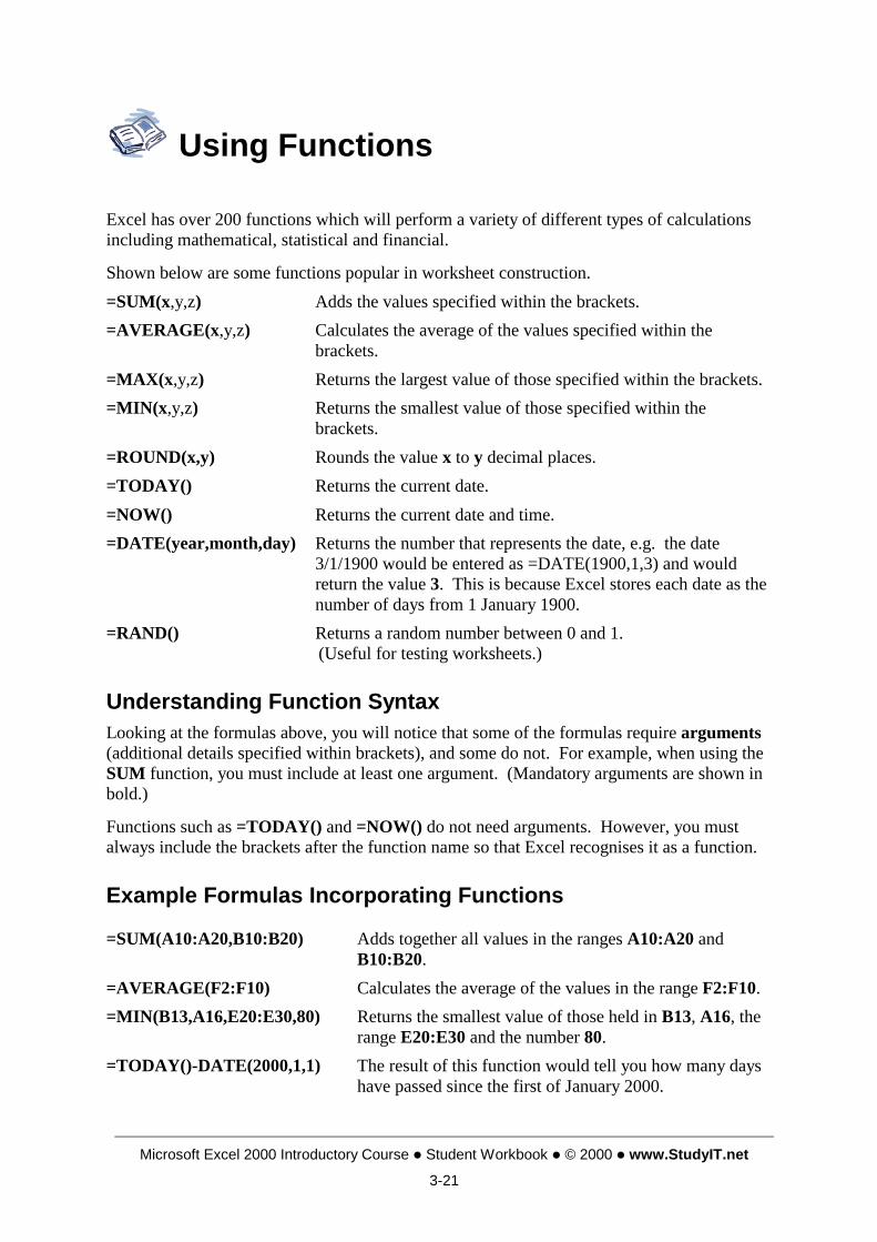
Using Functions

Excel has over 200 functions which will perform a variety of different types of calculations including mathematical, statistical and financial.

Shown below are some functions popular in worksheet construction. =SUM(x,y,z) Adds the values specified within the brackets. =AVERAGE(x,y,z) Calculates the average of the values specified within the

brackets. =MAX(x,y,z) Returns the largest value of those specified within the brackets. =MIN(x,y,z) Returns the smallest value of those specified within the

brackets. =ROUND(x,y) Rounds the value x to y decimal places. =TODAY() Returns the current date. =NOW() Returns the current date and time. =DATE(year,month,day) Returns the number that represents the date, e.g. the date

3/1/1900 would be entered as =DATE(1900,1,3) and would return the value 3. This is because Excel stores each date as the number of days from 1 January 1900.

=RAND() Returns a random number between 0 and 1. (Useful for testing worksheets.)

Understanding Function Syntax Looking at the formulas above, you will notice that some of the formulas require arguments (additional details specified within brackets), and some do not. For example, when using the SUM function, you must include at least one argument. (Mandatory arguments are shown in bold.)

Functions such as =TODAY() and =NOW() do not need arguments. However, you must always include the brackets after the function name so that Excel recognises it as a function.

Example Formulas Incorporating Functions

=SUM(A10:A20,B10:B20) Adds together all values in the ranges A10:A20 and B10:B20.

=AVERAGE(F2:F10) Calculates the average of the values in the range F2:F10. =MIN(B13,A16,E20:E30,80) Returns the smallest value of those held in B13, A16, the

range E20:E30 and the number 80. =TODAY()-DATE(2000,1,1) The result of this function would tell you how many days

have passed since the first of January 2000.


Using Functions

Nesting Functions When a formula contains two functions, the second should not be preceded by an = (equals) sign. However, every function in the formula must be followed by its brackets. For example, =ROUND(RAND()*10000,1).

This formula will multiply the number generated by the =RAND() function by 10000 then round the result to 1 decimal place.

Creating a Formula That Incorporates a Function A function can be an entire formula or it can be only part of a formula as seen in the example given above.

You can type the formula, including the function, directly into a cell, or you can add the function using the formula palette.

To Add a Function Using the Formula Palette 1. Move the active cell pointer to the cell that is to contain the formula. 2. Type the formula and, when ready to insert the function, click on the

Edit Formula button shown on the Standard toolbar and the formula bar. The formula palette will be displayed.

3. Select a function from the Function drop-down list at the left of the formula bar. If the function you want isn't on the list, select the More Functions option.

The Paste Function dialogue box will be displayed. /..


Using Functions

../ To Add a Function Using the Formula Palette Note: You can also display the Paste Function dialogue box by selecting the Insert,

Function menu option. When you select a function name, its syntax and a description of its use are displayed

below the left list box. In the illustration overleaf, the SUM function has been selected. Click OK to return to the formula palette.

Whether you chose from the list or the dialogue box, the outline of the function is entered into the formula, shown in the formula bar.

5. Complete the function: a) If the first argument is a cell range, define it either by typing it into the number1 text

box, or by clicking and dragging over the required range. Otherwise, type the first argument into the number 1 text box.

Note: If the formula palette is displayed on top of the range that is to be selected, you can hide it by selecting the Hide Dialogue Box button. The dialogue box will then shrink to a single line below the formula bar. Select the range then click the Show Dialogue Box button to return to the formula palette.

b) Repeat step a) above until the required arguments have been defined. 6. When all the arguments have been defined, click the OK button. 7. Complete the formula then press [ENTER] to display its result.

HelpTip: If you don't know which function you need, you can ask the Office Assistant for help. While the Paste Function dialogue box is on the screen, either click the Office Assistant if it's displayed, or click the Office Assistant button in the dialogue box then ask for Help with this topic.


Exercise 3-9 1. Open the workbook Weather stored in the Excel 2000 Intro Exercises folder.

2. Follow the instructions below to use the =MAX() function to show the highest temperature reached during the fortnight. — Click on cell B21. — Type =MAX( — Select the range B5:B18. Notice that this range is added to the formula in the formula bar.

— Type ) and press the [ENTER] key to complete the formula. The highest temperature, 10, is displayed in the cell.

3. Into cell B22, enter a formula that uses the =MIN() function to return the lowest temperature reached during the fortnight. The correct result is 0.

4. Into cell B23, enter a formula that uses the =AVERAGE() function to find the average temperature for the fortnight. The correct result is 5.78571.


Exercise 3-9 5. Following the instructions below, use the formula palette to insert a =MAX() function that

will return the highest number of Sunshine Hrs on any single day during the fortnight. — Click on cell C21 then click on the Edit Formula button shown on the Standard

toolbar. — Click on the Function drop-down arrow then select the Max function.

This function is shown in the formula bar and the formula palette expands to show the function, its arguments and a description.

The first argument in this instance is the cell reference C5:C18. — As this range isn't entirely visible, click the Hide Dialog Box button to shrink the

formula palette then click and drag over the range C5:C18. — Click the Show Dialog Box button to display the formula palette again.


Exercise 3-9 — As no other arguments are required, click on the OK button to complete the formula. The correct result is 8.

6. Following the instructions below, add a =MIN() function to the formula palette that will return the lowest number of Sunshine Hrs into cell C22. — Click on cell C22 then click on the Edit Formula button shown on the Standard

toolbar. — Click on the Function drop-down arrow then select More Functions. The Paste Function dialogue box will be displayed.

— Select Statistical from the Function category list. — Select MIN from the Function name list. — Click OK to return to the formula palette. — Complete the function as described in step 5.

The correct answer is 4.

7. Using the formula palette add an =AVERAGE() function that will return the average number of Sunshine Hrs into cell C23.

The correct answer is 5.935714286.

8. Use the AutoFill handle to copy the formulae to columns D and E.


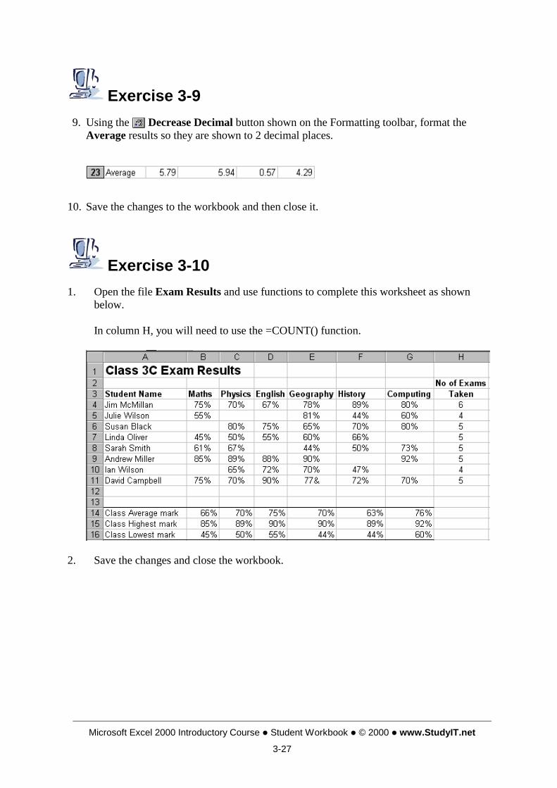
Exercise 3-9 9. Using the Decrease Decimal button shown on the Formatting toolbar, format the

Average results so they are shown to 2 decimal places.

10. Save the changes to the workbook and then close it.

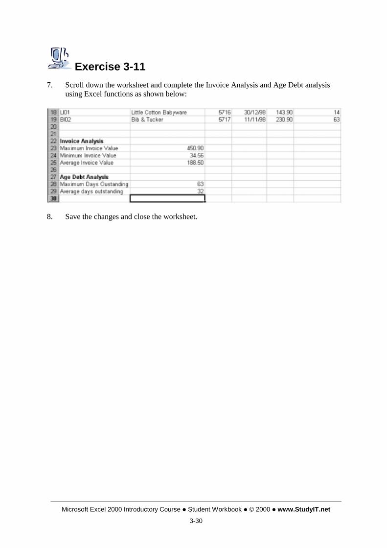
Exercise 3-10 1. Open the file Exam Results and use functions to complete this worksheet as shown

below. In column H, you will need to use the =COUNT() function.

2. Save the changes and close the workbook.


Working with Dates and Times

Working with Dates Excel will recognise an entry as a date if it is entered in one of Excel's acceptable date formats, e.g. 14/06/95 or 14-June-1995.

Although the entry will be shown in the worksheet as a date, it will be stored as a number. Each day is given a unique number equal to the number of days that have elapsed since 31st December 1899.

For example, 01/01/1900 is day 1, 01/02/1900 is day 32, and the example shown above, 14/06/95, is stored as day 34864.

Dates are stored in this way so that they can be used in calculations, so that, for example, you can subtract one date from another giving a number of days.

Initially, a date will be displayed in the format in which it was entered. However, the format can be changed using the Format, Cells command.

Note: British date formats such as dd/mm/yy, will be found in the Custom category in this dialogue box.

Working with Times If an entry is typed in the format hh:mm:ss, e.g. 15:05:40, it will be recognised as a time and displayed in the format in which it was entered.

Times are stored as the decimal fraction of the day that has elapsed since 23:59:59. So in a cell formatted as shown above, a time that is stored as 0.5 will be shown as 12:00:00, 0.25 as 06:00:00, 0.75 as 18:00:00 and so on.


Exercise 3-11 1. Open the file called Invoice Analysis. (Note that the dates relating to each invoice

shown on your computer screen will be different to those dates shown in these training notes.)

2. The =TODAY() function will display today's date. Enter =TODAY() into cell C1 and

you will see today's date displayed. 3. The =NOW() function will display the current date and time. Enter =NOW() into cell

D1 and you will see the current date and time displayed. (You may need to increase the column width to see the date and time displayed in full.)

4. In F4 enter the formula =TODAY()-D4. This will display how long this invoice has

been outstanding by subtracting the invoice date from today's date. Copy this function down column F.

5. Delete the contents of the cell range F4:F19 by selecting these cells and pressing [DELETE].

6. In F4, try entering the formula differently, this time making use of the =DATE(yyyy,mm,dd) function to enter today's date. Assuming today's date was the 1st of January 2000, the formula would ready: =DATE(2000,1,1)-D4. Create the formula you would need to show the number of day's outstanding from today's date and then copy that formula down the column.


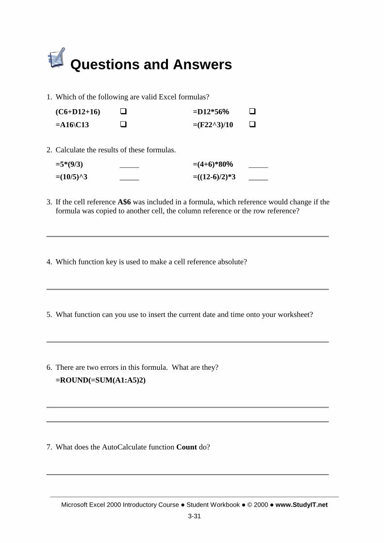
Exercise 3-11 7. Scroll down the worksheet and complete the Invoice Analysis and Age Debt analysis

using Excel functions as shown below:



Questions and Answers

1. Which of the following are valid Excel formulas?

(C6+D12+16) " =D12*56% "

=A16\C13 " =(F22^3)/10 " 2. Calculate the results of these formulas.

=5*(9/3) _____ =(4+6)*80% _____ =(10/5)^3 _____ =((12-6)/2)*3 _____

3. If the cell reference A$6 was included in a formula, which reference would change if the formula was copied to another cell, the column reference or the row reference?

4. Which function key is used to make a cell reference absolute?

5. What function can you use to insert the current date and time onto your worksheet?

6. There are two errors in this formula. What are they?

=ROUND(=SUM(A1:A5)2)

7. What does the AutoCalculate function Count do?


A2Z Index

A Absolute Cell Addressing, 3-13 AutoCalculate, 3-18 Average Function, 3-21

C Calculation Formulae, 3-3 Circular References, 3-4 Copying

formulae, 3-7

D Date Function, 3-21 Dates and Times, 3-28 Decimal Precision, 3-3

F Formulae

absolute cell addressing, 3-13 building, 3-3 copying, 3-7 creating, 3-2 creating circular references, 3-4 incorporating functions, 3-22 relative cell addressing, 3-7 rules for creating, 3-3

Functions average, 3-18, 3-21 count, 3-18 count nums, 3-18 date, 3-21 examples, 3-21 explained, 3-21 max, 3-18, 3-21 min, 3-18, 3-21 nesting, 3-22 now, 3-21 rand, 3-21 round, 3-21 sum, 3-18, 3-21 today, 3-21

M Mathematical Operators, 3-2 Max Function, 3-21 Min Function, 3-21

N Now Function, 3-21

R Rand Function, 3-21 Round Function, 3-21

S Sum Function, 3-21

T Times and Dates, 3-28 Today Function, 3-21

ABCDEFGHIJKLMNOPQRSTUVWXYZ

Documents

Section 3 - LogintoLearn - your gateway to learning in … 3 Topics Covered" Calculating using formulas..... 3-2 " Copying formulas..... 3-7 " Using absolute cell addresses ..... 3-13