SECTION 16 POWER-SYSTEM STABILITY - WordPress.comMay 16, 2011 · Power-system stability calculations fall into three major categories: transient, steady-state, and voltage stability

SECTION 16

POWER-SYSTEM STABILITY

Alexander W. Schneider, Jr.Senior Engineer

Mid-America Interconnected Network

Peter W. SauerProfessor of Electrical Engineering

University of Illinois at Urbana-Champaign

Introduction . . . . . . . . . . . . . . . . . . . . . . . . . . . . . . . . . . . . . . . . 16.1

Dynamic Modeling and Simulation . . . . . . . . . . . . . . . . . . . . . . . . . . 16.2

Transient Stability Analysis . . . . . . . . . . . . . . . . . . . . . . . . . . . . . . . 16.7

Single Machine– Infinite Bus Illustration . . . . . . . . . . . . . . . . . . . . . . . 16.8

Selecting Transient Stability Design Criteria . . . . . . . . . . . . . . . . . . . . . 16.13

Transient Stability Aids . . . . . . . . . . . . . . . . . . . . . . . . . . . . . . . . . 16.17

Selection of an Underfrequency Load-Shedding Scheme . . . . . . . . . . . . . 16.22

Steady-State Stability Analysis . . . . . . . . . . . . . . . . . . . . . . . . . . . . 16.24

Voltage Stability Analysis . . . . . . . . . . . . . . . . . . . . . . . . . . . . . . . 16.24

Data Preparation for Large-Scale Dynamic Simulation . . . . . . . . . . . . . . 16.27

Model Validation . . . . . . . . . . . . . . . . . . . . . . . . . . . . . . . . . . . . . 16.30

Bibliography . . . . . . . . . . . . . . . . . . . . . . . . . . . . . . . . . . . . . . . 16.34

INTRODUCTION

Power-system stability calculations fall into three major categories: transient, steady-state,and voltage stability. Transient stability analysis examines the power-system response tomajor disturbances, such as faults or loss of generation. This analysis is typically nonlin-ear and focuses heavily on the ability of the system generators to maintain synchronism.Steady-state stability analysis examines the qualitative nature of steady-state equilibriumin response to infinitesimally small disturbances. This analysis uses a linear version of thedetailed dynamic models and focuses on the eigenvalues of the linear system and theresponse of control systems. In earlier literature, steady-state stability was frequentlyreferred to as dynamic stability. Voltage stability analysis examines the ability of a powersystem to maintain acceptable voltage levels in response to both abrupt and gradual distur-bances. This analysis primarily uses steady-state modeling, although some analysis mayconsider dynamics of voltage controls such as tap-changing-under-load transformers.

16.1

16.2 HANDBOOK OF ELECTRIC POWER CALCULATIONS

The first procedure presented is the formulation of models that are utilized for stabilityanalysis. Using these modeling techniques, the remaining procedures illustrate bothsmall- and large-scale stability calculations. The small-scale procedures are provided toillustrate the mathematical steps associated with the analysis. The large-scale proceduresprovide the necessary considerations to perform this analysis on realistic system models.

DYNAMIC MODELING AND SIMULATION

Since power-system stability analysis is based on computations involving mathematicalmodels, it is important to understand the formulation of these models as well as their lim-itations. In the dynamic analysis of the fastest transients, partial differential equationsdescribing the properties of transmission lines are solved using approximate numericaltechniques. For the analysis presented in this chapter, the fast dynamics associated withthe synchronous machine stator, transmission lines, and loads are neglected. As such, theyare normally modeled with algebraic equations that are essentially identical to theirsteady-state form. The models of the synchronous generators and their controls are nor-mally limited to ordinary differential equations that are coupled to one another throughthe algebraic equations of the network. Each such differential equation expresses the de-rivative of a state variable, such as rotor angle, field voltage, or steam-valve position, interms of other states and algebraic variables. This section illustrates the procedures usedto create a typical model suitable for both transient and steady-state stability in a timeframe that neglects the high-frequency “60-Hz” transients.

It should be noted that the differential equations are generally nonlinear. In addition toproduct nonlinearities, phenomena such as magnetic saturation, voltage and valve-travellimits, dead bands, and discrete time delays are inherent in many of the devices modeled,and contemporary simulation packages provide a rich assortment of features to deal withthose deemed significant.

Calculation Procedure

1. Specify a Synchronous Machine Model that Captures the Dynamics of Interest

A synchronous machine has essentially three fundamental characteristics that need tobe represented in the dynamic model. These are the field winding dynamics, the damperwinding dynamics, and the shaft dynamics. In that order, the following model includes thefield flux-linkage dynamic state variable, , a single q-axis damper winding-flux linkagestate variable, , the shaft-position state variable relative to synchronous speed, �, and theshaft-speed state variable, �. The two flux-linkage states are shown in per unit (p.u.). Themodel indexes the equations for a system with m synchronous machines.

The first equation is the dynamic model that represents Faraday’s law for the field wind-ing, and Efd is the field-winding input voltage in per unit. This field voltage is taken either asa constant or a dynamic state variable in the exciter model, described next. The second equa-tion is the dynamic model that represents Faraday’s law for the q-axis damper winding. Thethird and fourth equations are Newton’s second law for the dynamics of the rotating shaft.

T �qoi dE�di

dt� �E�di � (Xqi � X�qi)Iqi i � 1, . . . , m

T �doi dE�qi

dt� �E�qi � (Xdi � X�di)Idi � Efdi i � 1, . . . , m

E�d

E�q

POWER-SYSTEM STABILITY 16.3

The inertia constant, H, represents the scaled total inertia of all masses connected intandem on the same shaft. The units of this constant are seconds. The X parameters areinductances that have been scaled with synchronous frequency (�o) to have the units ofreactance in per unit. The time constants multiplying the state derivatives have the unitsof seconds. The algebraic variables, Idi and Iqi , are components of the generator current,which in steady-state is a fundamental-frequency phasor with the following form:

During transients, the generator terminal current algebraic variables, Idi and Iqi, are relatedto the generator terminal voltage, Vej�, and the dynamic states through the followingstator algebraic equation (for i � 1, . . . , m):

The variable, TM, is the mechanical torque that may be a dynamic state variable in theprime mover and governor model, as described next, or a constant.

2. Specify an Exciter and Voltage Regulator Model that Captures the Dynamics ofInterest

Field current for a synchronous generator is normally supplied by a variable-voltageexciter whose output is controlled by a voltage regulator. The voltage regulator may beelectromechanical or solid state, and the exciter may be a direct-current generator, analternating-current generator with controlled or uncontrolled diodes to rectify the output,or a transformer with controlled rectifiers. The exciter and its voltage regulator are collec-tively referred to as an excitation system. While the exciter of a synchronous generator isnormally thought of as a mechanism for changing the terminal voltage, its action alsoindirectly determines the generator reactive power output.

IEEE task forces have periodically issued recommendations for the modeling of excitationsystems in dynamic studies. The first such effort suggested four models, of which model 1was applicable to the largest group of machines, those with continuously acting voltage regu-lators and either direct-current or alternating-current rotating exciters. Although more special-ized models represent these machines more rigorously, this model is still in widespread use,particularly for machines at some distance from the disturbances to be studied. An IEEE Type1 excitation system is modeled with three or four dynamic state variables as follows:

• Vsi: the voltage-sensing circuit output, whose time constant is generally quite small andoften assumed to be zero.

• VRi: the voltage regulator output.

• Efdi: the output of the exciter, which is the input to the synchronous-machine fieldwinding.

• Rfi: a rate-feedback signal, which anticipates the effect of the error signal in changingthe terminal voltage.

�� 1

Rsi � jX�di� Vie j�i

(Idi � jIqi) e j(�i�/2) � � 1

Rsi � jX�di� [E�di � (X�qi � X�di)Iqi � jE�qi]ej(�i�/2)

(Idi � jIqi) e j(�i�/2) i � 1, . . . , m

2Hi

�o

d�i

dt� TMi � E�diIdi � E�qi Iqi � (X�qi � X�di)IdiIqi i � 1, . . . , m

d�i

dt� �i � �o

i � 1, . . . , m


The equations for the derivatives of these state variables are

There is generally a limit constraint on the regulator output:

The input to the voltage-sensing circuit is the error signal, Vrefi � Vi. If TRi is zero, thenthis difference equals VSi, which becomes an algebraic variable rather than a dynamicstate variable. This is the difference between the desired or reference value of terminalvoltage and the measured value (typically line-to-line in per unit).

3. Specify a Prime Mover and Governor Model that Captures the Dynamics of Interest

Most modern generators have a governor, which compares their speed with synchronousspeed. This governor adjusts the flow of energy into the prime mover by means of a valve. Thevalve regulates steam flow in the case of a steam turbine, water in the case of a hydro unit, andfuel in the case of a combustion turbine or diesel engine. The prime mover fundamentally dic-tates the choice of governor model, and only that for a basic steam turbine will be discussed indetail. Models of hydro turbines must consider the dynamics of fluid flow in the penstock andsurge tank, if present. Models of combustion turbines must consider temperature limits asaffected by ambient conditions. Under significant perturbations these involve nonlinearities,which should not be neglected and are not amenable to a generalized treatment. At this time,there is no IEEE Standard recommending governor modeling. It is not uncommon to disregardgovernor response and assume constant mechanical power in screening or preliminary studies,and, in general, the conclusions reached by doing so will be conservative because the mechani-cal power input to the unit will be higher than if the governor response was modeled.

A simple prime mover and governor model having two dynamic state variables couldrepresent delays introduced by the steam-valve operating mechanism and the steam chestas follows. The variables are

• PSVi: the steam valve position

• TMi: the mechanical torque to the shaft of the synchronous generator

The equations for the derivatives of these state variables are

with the limit constraint

i � 1, . . . , m0 PSVi P maxSVi

TCHi dTMi

dt� �TMi � PSVi i � 1, . . . , m

TSVi dPSVi

dt� �PSVi � PCi �

1

RDi

� �i

�o� 1� i � 1, . . . , m

V minRi VRi V max

Ri i � 1, . . . , m

TFi dRfi

dt� �Rfi �

KFi

TFi

Efdi i � 1, . . . , m

TEi dEfdi

dt� �[KEi � SEi(Efdi)]Efdi � VRi i � 1, . . . , m

TAi dVRi

dt� �VRi � KAiRfi �

KAiKFi

TFi

Efdi � KAiVSi i � 1, . . . , m

TRi dVSi

dt� �VSi � (Vref i � Vi) i � 1, . . . , m


The input to the governor is the speed error signal, which is given here as the differ-ence between rated synchronous speed and actual speed. Notice that measuring all quan-tities within the model using a per-unit system permits using power and torque in thesame equation, as rated speed of 1.0 is used as the scaling factor.

Large steam turbine units may have up to four stages through which the steam passesbefore it returns to the condenser. If there are two or three stages, steam from the boilerinitially enters a high-pressure turbine stage. Steam leaving the first stage returns to a re-heater section within the boiler. After reheating, the steam enters the second turbine stage.The dynamic response of such “reheat” units is generally dominated by the time constantof this reheater, typically 4 to 10 s. Units that are at or near the maximum size for thevintage when they were built are often built as cross-compound units with two separateturbines and two generators. Steam from the boiler initially enters a high-pressure turbinestage, returns to the reheater, passes through an intermediate-pressure stage on the sameshaft as the high-pressure stage, and then crosses over to a low-pressure stage on the othershaft. The high-pressure and low-pressure machine rotor angles will vary considerablyfrom each other, because the former tend to have lower inertia and the low-pressure unitinput steam flow is subject to reheater and crossover piping lags.

4. Specify a Network/Load Model that Captures the Dynamics of Interest

In order to complete the dynamic model, it is necessary to connect all of the synchronousgenerators through the network to the loads. In most studies all fast network and load dy-namics are neglected, so this model consists of Kirchhoff’s power law at each node (alsocalled bus). It is common to characterize the initial real and reactive load at each bus as aparticular mix of constant power, constant current, and constant impedance load with respectto voltage changes at that bus. The proportions will depend on the nature of the loads (resi-dential, agricultural, commercial, or industrial) anticipated under the conditions being mod-eled. The proportions of interest are the short-time responses of load to a voltage change;longer-term dynamics such as load tap-changer operation and reduced cycling of thermostat-ically controlled heating or cooling loads are not normally modeled. If single, large synchro-nous or induction motors comprise a significant proportion of the load at a bus near a distur-bance being simulated, their dynamics should be modeled in a manner similar to generators.

The following algebraic equations give these constraints both for the synchronousmachine stator and the interconnected network. The variable indexing assumes that the msynchronous machines are each at a distinct network node and that there are a total of nnodes in the network. (Loads are “injected” notation.) The i-kth entry of the bus admit-tance matrix has magnitude Y and angle �.

i � 1, . . . , m

i � m � 1, . . . , n

For given functions PLi(Vi) and QLi(Vi), the n � m complex algebraic equations mustbe solved for Vi, �i (i � 1, . . . , n), and Idi, Iqi (i � 1, . . . , m) in terms of states, �i,E�di, and E�qi (i � 1, . . . , n). The currents can clearly be explicitly eliminated by solvingthe m stator algebraic equations (linear in currents) and substituting into the differential

PLi(Vi) � jQLi (Vi) � �n

k�1ViVkYike j(�i��k��ik)

� �n

k�1ViVkYik ej(�i��k��ik)

Vi e j�i (Idi � jIqi) e

�j(�i�/2) � PLi(Vi) � jQLi(Vi)

�[E�di � (X�qi � X�di)Iqi � jE�qi] e j(�i�/2) i � 1, . . . , m

0 � Vi e j�i � (Rsi � jX�di)(Idi � jIqi) e

j(�i�/2)


equations and remaining algebraic equations. This leaves only the n complex network al-gebraic equations to be solved for the n complex voltages, .

5. Compute Initial Conditions for the Dynamic Model

In dynamic analysis it is customary to assume that the system is initially in sinusoidalconstant-speed steady-state. This means that the initial conditions can be found by settingthe time derivatives in the preceding model equal to zero. The steady-state condition thatforms the basis for the initial conditions begins with the solution of a standard powerflow. From this, the steps to compute the initial conditions of the two-axis model formachine i are as follows:

Step 1. From an initial power flow, compute the generator terminal currents, , as(PGi � jQGi) /Vi e�j�i.

Step 2. Compute �i as angle of [Vie j�i � jXqiIGie j� i].

Step 3. Compute �i � �o.

Step 4. Compute Idi, Iqi from (Idi � jIqi) � IGie j(�i��i�/2).

Step 5. Compute E�qi as E�qi � Vi cos (�i � �i) � X�di Idi � RsiIqi.

Step 6. Compute Efdi as Efdi � E�qi � (Xdi � X�di)Idi.

Step 7. .

Step 8. Compute VRi as VRi � [KEi � SEi(Efdi)]Efdi.

Step 9. Compute E�di as E�di � (Xqi � X�qi)Iqi.

Step 10.

Step 11. Compute Vrefi as Vrefi � VSi � Vi.

Step 12. Compute TMi as TMi � E�diIdi � E�qi Iqi � (X�qi � X�di)Idi Iqi.

Step 13. Compute Pci and Psvi as Pci � Psvi � TMi.

Step 14. As an additional check, verify that all dynamic model states defined by these ini-tial conditions are within relevant limits and that all state derivatives are zero.This ensures that the specified initial condition is attainable and is in equilibrium.

This computational procedure is unique in that the control inputs for generator terminalvoltage and turbine power are not specified. Alternatively, the generator terminal voltageand terminal power are specified in the power flow, and the resulting current is used tocompute the required control inputs.

6. Specify the Disturbance(s) to Be Simulated

The purpose of a dynamic simulation is to predict the behavior of the system in responseto some disturbance or perturbation. This disturbance could be any possible change in theconditions that were used to compute the initial steady state. Transient stability studies nor-mally consider disturbances such as a fault of a specified type (e.g., single-phase to ground)and duration, the loss of a generating unit, the false trip of a line, the sudden addition of aload, or the change of a control input. This disturbance is normally modeled by a change in

Compute VSi as VSi �VRi

KAi

.

Compute Rfi as Rfi �KFi

TFi

Efdi

IGiej�

i

Viej�i


one or more of the constants specified in the dynamic model. Steady-state stability studiesconsider response to smaller but more frequent perturbations, such as the ramping up anddown of system loads over the operating day. Voltage stability studies consider both suchsmall perturbations and system changes such as the loss of a generating unit or line, butgenerally do not consider conditions during faults. Additional information on this step of theprocedure is discussed next in the description of the various stability analyses.

TRANSIENT STABILITY ANALYSIS

Transient stability analysis is concerned with simulating the response of the power systemto major disturbances. The primary objective of the analysis is to determine if all syn-chronous machines remain in synchronism after a fault or other disturbance. A secondaryobjective is to determine if the nonlinear dynamic response is acceptable. For example,the bus voltages during the transient must remain above acceptable transient levels. Whilethese transient levels are considerably below steady-state acceptable levels, they must bemonitored at each instant of the simulation. This analysis is normally done throughdynamic simulation using a detailed dynamic model and numerical integration. The out-put of this simulation includes synchronous-machine rotor angle and bus voltage trajecto-ries as a function of time. For a typical case where the disturbance is a fault, the analysisincludes the following procedures.


1. Compute the Prefault Initial Conditions

Prepare the case data and solve a power-flow problem that gives all of the prefault busvoltages and generator currents. This involves the solution of the network power-balanceequations for specified values of generator voltage magnitudes and real-power outputs.From this power-flow solution, the initial conditions for all dynamic state variables arecomputed using the procedure provided earlier.

2. Modify the System Model to Reflect the Faulted Condition

The faulted condition is usually modeled as a modification to the system bus-admit-tance matrix which makes up a portion of the algebraic equations of the dynamic modelgiven earlier. The fault impedance, computed using symmetrical component theory, isadded as a shunt admittance to the diagonal element of the faulted bus.

3. Compute the System Trajectories while the Fault Is On

With the modification of the admittance matrix, the solution of the algebraic-differen-tial equation model will now produce changes in algebraic variables such as voltage andcurrent. These changes disturb the equilibrium, so the derivatives of the state variables areno longer zero. Solution for the time series of values of each state, termed its trajectory,is obtained using a numerical integration technique. The solution continues until the pre-specified fault clearing time.

Changes in the states over time will in turn impact the algebraic variables describing theremainder of the power system. There are basically two approaches used in power-systemsimulation packages: Simultaneous-Implicit (SI) and Partitioned-Explicit (PE). The SImethod solves both the differential and algebraic equations simultaneously using an implicitintegration routine. A typical integration routine is the trapezoidal method, which resultsin the need to solve a set of nonlinear algebraic equations at each time step for the new


dynamic states—hence the name implicit. Since the algebraic equations of a power systemare also nonlinear, it is efficient to solve these together—hence the name simultaneous. Thesolution of the model at each time step is performed using Newton’s method, with an initialguess equal to the solution obtained at the converged solution of the previous time step.

The PE method solves the differential and algebraic equations in separate steps. Thedifferential equations are first solved using an explicit integration scheme (such asRunge-Kutta) that directly gives the new dynamic states in terms of the old dynamicstates and the old algebraic states. Since this method considers the algebraic variablesto be constant at their previous time-step value, this method is noniterative — hence, thename explicit. After the dynamic states are computed for the new time, the nonlinearalgebraic equations are solved iteratively using the dynamic states as constants. Thisgives the algebraic states for the new time. Since the solution of the dynamic and alge-braic equations is done separately, this is called a partitioned solution. This PE methodis typically less numerically stable than the SI method. Since the algebraic equationsare nonlinear, the PE method is still iterative at each time step even though an explicitintegration routine is used.

4. Remove the Fault at the Prespecified Fault Clearing Time

When the numerical integration routine attains the prespecified clearing time, the sys-tem admittance matrix is modified again to reflect the specified postfault condition. Thiscould be simply the removal of the fault itself or the removal (or change in degree, asfrom three-phase to phase-to-ground) of the fault plus the removal of a line or generatingunit— simulating the action of protective relaying and circuit breakers.

5. Compute the Postfault System Trajectories

With the modified system-admittance matrix, the numerical integration routine continuesto compute the solution of the differential-algebraic equations. This solution is usually con-tinued to a specified time, unless the system is deemed unstable because one or moremachine rotor angles have exceeded a specified criterion, such as 180 , with respect to eithera synchronous reference or to other, less-perturbed machines. An unstable system normallycontains trajectories that increase without bound. However, if all of the trajectories of thesynchronous machine angles increase without bound, the system may be considered stable inthe sense that all machines are remaining in synchronism, although the final speed may notbe rated synchronous speed. Alternatively, a solution may be terminated because one or moreof the trajectories is unacceptable, that is, voltage dips below acceptable transient levels.

Related Calculations. If the system is found to be stable in Step 5, Steps 3 to 5 can berepeated with a larger prespecified clearing time. When an unstable system is encoun-tered, the clearing time has exceeded the “critical clearing time.” Determining the exactvalue of the critical clearing time can be done by repeated simulations with various pre-specified clearing times.

SINGLE MACHINE–INFINITEBUS ILLUSTRATION

To illustrate several of these stability calculations, several major simplifying assumptionsare made to the machine dynamic model. In the dynamic model given earlier, assume

1. Tdo� � T �qo � �. This makes the machine dynamic states, Eq� and Ed�, constants andremoves the exciter from consideration.


2. X�q � X�d. This greatly simplifies the machine torque and circuit model.

3. TCH � TSV � �. This makes the governor dynamic states, TM and PSV, constants.

4. Rs � 0. This greatly simplifies the machine power model.

With these assumptions, the dynamic model of a synchronous machine is greatly simpli-fied to be

where Pe is the real power out of the machine and Pm is the constant input power from theturbine. The algebraic equations for the machine simplify to

Subtracting the appropriate constant from each angle, this can be written as the classicalcircuit model:

where V�is the constant voltage magnitude behind transient reactance and Ve is the ter-minal voltage. This classical dynamic model is used in the following illustration.1

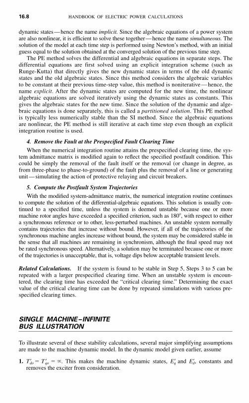
The equivalent network of a synchronous machine connected to an infinite bus isshown in Fig. 16.1. All quantities in Fig. 16.1 are given per unit, and the impedance val-ues are expressed on a 1000-MVA base. The machine operates initially at synchronousspeed (377 rad/s on a 60-Hz system). A three-phase fault is simulated by closing switchS1 at time t � 0. S1 connects the fault bus F to ground through a fault reactance Xf . Com-pute the machine angle and frequency for 0.1s after S1 is closed. Compute the machineangle and frequency with Xf � 0 and 0.15 p.u.

j�v

V� e j� � jX�d Ie

j�I � Ve j�v

[E�d � jE�q]e j(��/2) � �jX�d (Id � jIq)e

j(��/2) � Ve j�

2H�o

d�dt � Pm � Pe

d�

dt� � � �o

FIGURE 16.1 Equivalent network of single machine connected to an infinitebus. All quantities are per unit on common 1000-MVA base.

1 Originally presented in a previous edition of this chapter by Cyrus Cox and Norbert Podwoiski.



1. Compute the Initial Internal Machine Angle

Use �0 � sin�1 (Pe0Xtot /V�Vl), where �0 � initial internal machine angle with respect tothe infinite bus (for this machine, �0 is the angle of the voltage V�), Pe0 � initial machineelectrical power output, V� � voltage behind transient reactance X�d, Vl � infinite-bus volt-age, and Xtot � total reactance between the voltages, V� and Vl. Thus, �0 � sin�1 [(0.9)(0.3 � 0.125 � 0.17)/(1.0)(1.0)] � 32.4°.

2. Determine Solution Method

Computing synchronous-machine angle and frequency changes as a function of timerequires the solution of the swing equation d�2 /dt2 � (�0 /2H)(Pm � Pe), where � �internal machine angle with respect to a synchronously rotating reference (infinite bus),�0 � synchronous speed in rad/s, H � per-unit inertia constant in s, t � time in s,Pm � per-unit machine mechanical shaft power, and Pe � per-unit machine electric-power output. The term (Pm � Pe) is referred to as the machine accelerating power andis represented by the symbol, Pa .

If Pa can be assumed constant or expressed explicitly as a function of time, then theswing equation will have a direct analytical solution. If Pa varies as a function of �, thennumerical integration techniques are required to solve the swing equation. In the net-work of Fig. 16.1, for Xf � 0 the voltages at bus F and Pe during the fault are zero. Thus,Pa � Pm � constant, and therefore with Xf � 0, there is a direct analytical solution to theswing equation. For the case in which Xf � 0.15 (or Xf � 0), the voltages at bus F andPe during the fault are greater than zero. Thus, Pa � Pm � Pe � a function of �. There-fore, with Xf � 0.15, numerical integration techniques are required for solution of theswing equation.

3. Solve Swing Equation with Xf � 0

Use the following procedure:

a. Compute the machine accelerating power during the fault. Use Pa � Pm � Pe; forthis machine, Pm � Pe0 � 0.90 p.u.; Pe � 0. Thus, Pa � 0.90.

b. Compute the new machine angle at time, t � 0.1 s. The solution of the swing equa-tion with constant Pa is � � �0 � (�0 /4H) Pat 2, where the angles are expressed inradians and all other values are on a per-unit basis. Thus,

� 0.735 rad, or 42.1°

c. Compute the new machine frequency at time, t � 0.1 s. The machine frequency isobtained from the relation, � � d� /dt � �0, where d� /dt � (�0Pat)/2H. Thus, � �[(377)(0.90)(0.1)/(2)(5)] � 377 � 380.4 rad/s, or 60.5 Hz.

It is obvious from the equation for � in Step b that the rotor angle will increase indefi-nitely as long as the fault is on, indicating instability.

4. Solve Swing Equation with Xf � 0.15 p.u.

Use the following procedure.

a. Select a numerical integration method and time step. There are many numericalintegration techniques for solving differential equations including Euler, modified

� � � 32.4

57.3 / rad � � � 377

4 � 5 � 0.90(0.1)2


Euler, and Runge-Kutta methods. The Euler method is selected here. Solution byEuler’s method requires expressing the second-order swing equation as two first-orderdifferential equations. These are: d� /dt � �(t) � �0 and d� /dt � (�0Pa(t))/2H. Euler’s method involves computing the rate of change of each variable at thebeginning of a time step. Then, on the assumption that the rate of change of eachvariable remains constant over the time step, a new value for the variable is com-puted at the end of the step. The following general expression is used: y(t � �t) �y(t) � (dy /dt)�t, where y corresponds to � or � and �t � time step and y(t) anddy /dt are computed at the beginning of the time step. A time step of 1 cycle(0.0167 s) is selected.

b. From Fig. 16.2, determine the expression for the electrical power output during thistime step. For this network, Case 3 is used, where XG � X�d � XGSU � 0.3 �0.125 � 0.425 p.u., Xs � 0.17, and Xf � 0.15. Thus,

Pe � [(1.0)(1.0) sin �] �{0.424 � 0.17 � [(0.425)(0.17)/0.15]}

� 0.93 sin �

c. Compute Pa(t) at the beginning of this time step (t � 0 s). Use Pa(t) � Pm � Pe(t)for t � 0, where Pm � Peo0 � 0.90 p.u.; Pe(0) � 0.930 sin 32.4°. Thus, Pa(t �0) � 0.90 � 0.93 sin 35.2° � 0.40 p.u.

d. Compute the rate of change in machine variables at the beginning of the time step(t � 0). The rate of change in the machine phase angle d� /dt � �(t) � �0 for t �0, where �(0) � 377 rad/s. Thus, d� /dt � 377 � 377 � 0 rad/s. The rate ofchange in machine frequency is d� /dt � �oPa(t) /2H for t � 0, where Pa(0) �0.40 p.u. as computed in c. Thus, d�/dt � (377)(0.40)/(2)(5) � 15.08 rad/s2.

e. Compute the new machine variables at the end of the time step (t � 0.0167 s). Thenew machine phase angle is �(0.0167) � �(0) � (d� /dt)�t, where the angles are

FIGURE 16.2 Power-angle relations for general network configurations; resistances areneglected. VG � internal machine angle, XG � machine reactance, Xs � system reactance,Pe � machine electrical power output, VI � infinite bus voltage, and Xf � fault reactance.�0º

��


expressed in radians and �t � time step � 0.0167 s. Thus, �(0.0167) �32.4° / (57.3° / rad) � (0)(0.0167) � 0.565 rad, or 32.4°. The new machine frequencyis �(0.0167) � �(0) � (d� /dt)�t � 377 � (15.08)(0.0167) � 377.25 rad/s, or60.04 Hz.

f. Repeat c, d and e for the desired number of time steps. Table 16.1 displays theremaining calculations for the 0.1-s solution time. The machine frequency at 0.1 s � 378.48 rad/s, or 60.24 Hz; the corresponding machine angle is 36.0°.

Related Calculations. The preceding illustration simply computes the fault-on trajecto-ries for a time of 0.1 s. In an actual study, the simulation would need to be performedwell beyond the time that the fault is cleared to observe the responses to determine if theunit is stable for that fault-clearing time. If it is not stable, the calculation is repeatedwith successively smaller clearing times until a stable response is observed. The longestclearing time showing a stable response is called the critical clearing time. The proce-dure can readily be generalized to consider the case of a second switching step —forinstance, if only two of three breaker poles operate to clear a three-phase fault inprimary clearing time and the remaining phase-to-ground fault is cleared later by backupcircuit breaker operation.

The preceding example can readily be set up on a spreadsheet program such as Excel®

and the calculation extended sufficiently to demonstrate whether the machine will remainstable. The curves shown in Fig. 16.3 were produced by such an application, which isincluded as file swingcurve.xls on the diskette enclosed with this Handbook.* Selectedadditional cases are also presented; by changing the parameters in shaded cells, the usercan observe their effect on the plotted rotor angle curves.

There are direct methods that seek to determine this critical clearing time with lessnumerical integration effort and without repeated analysis with various clearing times.These methods are called equal area criteria, for single-machine systems, and directmethods for large-scale systems.

TABLE 16.1 Computations for Solution of Swing Equation by Euler’s Method

Time Frequency AngleAccel.

Derivatives Increments

Radians/ Radians power Angle Speed d� /dt d� /dt(s) second-� Hz � Degrees Pa (t) d� /dt d� /dt �t �t

0 377 60 0.564 32.4 0.402 0 15.14 0 0.2530.0167 377.25 60.04 0.564 32.4 0.402 0.253 15.14 0.0042 0.2530.0334 377.51 60.08 0.569 32.6 0.398 0.506 15.02 0.0084 0.2510.0501 377.76 60.12 0.577 33.1 0.392 0.757 14.77 0.0126 0.2470.0668 378.00 60.16 0.590 33.8 0.382 1.003 14.40 0.0168 0.2410.0835 378.24 60.20 0.606 34.8 0.369 1.244 13.91 0.0208 0.2320.1000 378.48 60.24 0.627 36.0 0.353 1.476 13.32 0.0247 0.222

Pa � 0.93 sin�, d� /dt � �(t) � �0

d� /dt � (�0Pa (t)) /2H, �t � 0.0167 s, � (t � �t) � � (t) � d� /dt �t� (t � �t) � � (t) � d� /dt �t

*See above-referenced file on accompanying CD for curves shown in Fig.16.3 and other selected cases.


SELECTING TRANSIENT STABILITYDESIGN CRITERIA

Stability design criteria may be deterministic or probabilistic. A deterministic criterionrequires that the generating unit be demonstrated to be stable for any disturbance of aspecified level of severity— for instance, any three-phase fault tripping a single transmis-sion system element in six cycles. Events of greater severity— say, faults cleared bybackup protection schemes in a greater time following initiation—are disregarded. Aprobabilistic criterion requires that the total annual frequency of events leading to insta-bility be less than a specified number or, equivalently, that the mean time to instability begreater than a certain number of years.2

Stability design criteria are to be selected for the generating facility shown in Fig.16.4. The design basis for the plant is that the mean time to instability (MTTI-failure dueto unstable operation) is greater than 500 years.

FIGURE 16.3 Rotor angle curves for stable and unstable cases with system as shown in Fig. 16.1. Faultduration is 36 cycles for the stable case and 37 cycles for the unstable case.

2 Example of application of probabilistic design criteria by Cyrus Cox and Norbert Podwoiski.



1. Specify a Fault-Exposure Zone

A fault-exposure zone defines a boundary beyond which faults can be neglected in theselection of the stability criteria. For example, on long out-of-plant transmission lines it istypically unnecessary to consider line faults at the remote end. Specifying a fault-expo-sure zone is generally based on the fault frequency and/or the magnitude of the reductionin the plant electric output during the fault.

For this plant, specify a fault-exposure zone of 50 km (31 mi); that is, it will beassumed that the plant will maintain transient stability to faults beyond this distance, evenif breaker failure delays fault clearing. In addition, faults in the switchyard are consideredoutside the fault-exposure zone. This is done because switchyard-fault frequency isgenerally much less than line-fault frequency.

2. Compute Fault Frequency within the Exposure Zone

Use Table 16.2 to estimate the fault frequency per line. The values given are very gen-eral and based on composite data from numerous power-industry sources. Line-fault fre-quency varies with factors such as line design, voltage level, soil conditions, air pollution,storm frequency, etc.

For this plant, use the typical line-fault frequency rates. Thus, the fault frequencywithin the exposure zone is f � (number of lines) (fault frequency) (exposure zone/

FIGURE 16.4 A two-unit generating facility, switch-yard, and out-of-plant transmission.

TABLE 16.2 Typical Extra-High Voltage (EHV) Probability Data

Data description Optimistic Typical Pessimistic

Line-fault frequency, faults /100 km, yr 0.62 1.55 3.1Conditional probability of relay failure to

sense or stuck breaker* 0.0002 0.003 0.01

* Assumes nonindependent pole tripping. For independent pole tripping, probabilities are for a 1 � failure.


100 km), where the fault frequency is in faults /100 km-yr and exposure zone is in km.Then f � (2)(1.55)(50/100) � 1.55 faults /yr within the exposure zone.

Use Table 16.3 to estimate the fault frequency on the basis of the number of phasesinvolved. For this plant, use the composite values and assume that the unknown fault typesconsist entirely of single-phase faults. Thus, the three-phase fault frequency f3� � (percentof total faults that involve (3�)( f ) � (0.03)(1.55) � 0.465 � 3� faults /yr, or 1/ f3� ��MTBF3� � mean time between 3� faults � 1/0.0465 � 21.5 yr. Similar calculationsare made for the other fault types and are tabulated next.

Fault type Faults per year MTBF, yr

Three-phase 0.0465 21.5Double-phase 0.140 7.17Single-phase (� unknown) 1.36 0.733

Note that in these calculations f � 1/MTBF. The precise relation for the frequencyis f � 1/(MTBF � MTTR), where MTTR � mean time to repair (i.e., time to clear thefault and restore the system to its original state). The term MTTR is required in theprecise relation because a line cannot fail while it is out of service. However, for sta-bility calculations, MTTR �� MTBF, and, thus, the approximation, f � 1/MTBF, isvalid.

3. Compute Breaker-Failure Frequencies

Only breaker failures in which both generating units in Fig. 16.4 remain connectedto the transmission system are considered. Tripping one unit at a multiunit plant sub-stantially improves the stability of the remaining units because they can utilize thetripped unit’s portion of the available power transfer. Intentional tripping of a generat-ing unit in the process of clearing a “stuck breaker” is sometimes used as a stabilityaid. For this plant and transmission system, the failure of breaker 2B for a fault on line1 will result in tripping unit 2. Thus, only three breaker failures affect stability: 2A,3B, and 3C.

From Table 16.2, the conditional probability that a relay /breaker will fail to senseor open for a line fault is pbf � 0.003 (typical value for nonindependent pole tripping).The frequency of a three-phase fault plus a breaker failure is f3�,bf � f3� pbf B, whereB � number of breaker failures that impact stability. Thus, f3�,bf � (0.465)(0.003)(3) �4.19 � 10� 4 three-phase faults plus breaker failures per year, or 1 / f3�,bf � 2390 yr.Similar calculations are made for the other fault types and are tabulated next.

TABLE 16.3 Composition of EHV Transmission-Line Faults

Percent of total faults

Type of fault 765 kV EHV composite 115 kV

Phase to ground 99 80 70Double-phase to ground 1 7 15Three-phase to ground 0 3 4Phase to phase 0 2 3Unknown 0 8 8

Total 100 100 100


Mean timeFault plus betweenbreaker faultsfailures plus breaker

Fault type per year failures, yr

Three-phase 0.000419 2390Double-phase 0.00126 793Single-phase (� unknown) 0.122 81.7

4. Select the Minimum Criteria

As a design basis, the plant must remain stable for at least those fault types for whichthe MTBF is less than 500 years. Thus, from the fault-type frequencies computed in Steps2 and 3, only a three-phase or two-phase fault plus breaker failure could be eliminated toselect the minimum criteria. A check is now made to ensure that neglecting three- andtwo-phase faults plus breaker failures is within the design basis.

5. Compute the Frequency of Plant Instability

Use fI � � frequencies of fault types eliminated in Step 4, where fI � frequency ofplant instability. Thus, fI � f3�,bf � f2�,bf � 0.000419 � 0.00126 � 0.00168 occurrencesof instability per yr, or 1/ fI � �mean time to instability � 595 yr. Thus, neglectingthree-phase and two-phase faults plus breaker failures in the criteria, the value is withinthe original design basis of MTTI � 500 yr. If the MTTI computed in this step was lessthan the design basis, then additional fault types would be added to the minimum criteriaand the MTTI recomputed.

6. Select the Stability Criteria

The following stability criteria are selected:

a. Three-phase fault near the plant’s high-voltage bus cleared normally

b. Single-phase fault near the plant’s high-voltage bus plus a breaker failure

If the plant remains stable for these two tests, the original design basis has been satisfied.

Related Calculations. Specifying a design basis, although not a step in the procedure, iscritical in selecting stability criteria. No general guidelines can be given for specifying adesign basis. However, most utilities within the United States specify some type ofbreaker failure test in their criteria.

In addition to neglecting low-probability fault types, low-probability operating condi-tions can also be neglected in the selection of stability criteria. As an example, supposethat for this plant it was determined that during leading power-factor operation, the plantcould not remain stable for a single-phase fault plus a breaker failure. Further assume thatthe plant transition rate into leading power-factor operation is � � 2 yr and the mean du-ration of each occurrence is r � 8 h. Use the following general procedure to compute themean time to instability.

1. Sketch a series-parallel event diagram as shown in Fig. 16.5a. Any break in thecontinuity of the diagram causes instability. A break in continuity could be caused byEvent 3 or 4, or the simultaneous occurrence of Events 1 and 2.

2. Reduce the series-parallel event diagram to a single equivalent event. By recursivelyapplying the relations in Fig. 16.6, the diagram can be reduced to an equivalent MTTI. To


FIGURE 16.5 Event diagrams. (a) Series-parallel event diagram. (b) Events 1 and 2reduced to equivalent event. (c) All four events reduced to a single event.

reduce the parallel combination of Events 1 and 2, use �12 � �1�2 (r1 � r2) (1 � �1r1 ��2r2), where �12 � equivalent transition rate for Events 1 and 2, �1 � transition rate forEvent 1 in occurrences per year, �2 � transition rate for Event 2 in occurrences per year(note that for this case, f2 � �2 � 0.122 occurrences per year as computed in Step 3), r1 �mean duration of Event 1 in years � 8 h (8760 h/yr) � 0.0009 yr, r2 � mean duration ofEvent 2 in years (the duration of a single-phase fault plus breaker failure � 0 yr). Thus,�12 � (2)(0.122)(0.0009)/[1�(2)(0.0009)] � 0.0002 transitions/yr. The diagram is nowreduced to Fig. 16.5b. Note that the equivalent duration of Events 1 and 2 is r12 � 0 yr.The equivalent transition rate for the three series events is �eq � �12 � �3 � �4 � 0.0002 �0.00126 � 0.000419 � 0.00188 occurrences/yr. Since req � 0 yr, we have �eq � feq �frequency of instability fI , or 1/ fI � MTTI � 1/0.00188 � 532 yr (Fig. 16.5c).

This general procedure can be used either to select a criterion or to determine the ade-quacy of final stability design.

TRANSIENT STABILITY AIDS3

If a generating facility such as that of Fig. 16.4 cannot meet the stability design criteriaand the number and configuration of transmission circuits is fixed, the following proce-dure is used to select a set of stability aids to meet the criteria.

3 This section was originally written by Cyrus Cox and Norbert Podwoiski for a previous edition.



1. Determine Critical Fault-Clearing Times for the System as Specified

Compute or use computer simulation to determine the critical fault-clearing times foreach contingency specified in the stability criteria.

2. Compute the Attainable Fault-Clearing Time

Table 16.4 displays the range of typical EHV (extra-high voltage) relay-breakerclearing times. Most components of the total clearing times are limited by the type of

FIGURE 16.6 Equivalent frequency-duration formulas for occurrence of eventsin series or parallel. *Although outage rate and frequency have same units of outageper year, they are not equivalent; � is the reciprocal of mean time to failure (MTTF);f is the reciprocal of the sum of the MTTF and mean time to repair (MTTR). IfMTTF � MTTR, then f � �.

TABLE 16.4 Range of Typical EHV Relay-Breaker Clearing Times

Time in cycles (60 Hz)

Function Fast Average Slow

Primary relay 0.25�0.5 1.0�1.5 2.0Breaker clearing 1.0 3.0 3.0�5.0Total normal clearing time 1.3�1.5 3.0�3.5 5.0�7.0Breaker-failure detection 0.25�0.5 0.5�1.5 1.0�2.0Relay coordination time 3.0 3.0�5.0 5.0�6.0Auxiliary relay 0.25�0.5 0.5�1.0 1.0Backup breaker clearing 1.0 2.0 3.0�5.0Total backup clearing 5.75�6.5 9.0�13.0 15.0�20.0


equipment used. The function most susceptible to reduction is the relay-coordinationtime for backup clearing. However, reduction in the coordination time can result inerroneous backup clearing. The minimum achievable times displayed in Table 16.4 areassociated with state-of-the-art equipment (1-cycle breakers and ultra-high-speedrelaying).

3. Modify Machine and GSU Transformer Parameters

A decrease in the machine transient reactance and /or an increase in the inertiaconstant can provide increases in CFC time. Table 16.5 displays typical ranges ofthese parameters for modem turbine generators. Table 16.6 displays the typical rangeof standard impedances for GSU transformers. The most common way to achieve CFCincreases in the generation system is to reduce the generator step-up transformer(GSU) impedance. GSU transformer impedances below the minimum standard canbe obtained at a cost premium. Reductions in GSU transformer impedance may belimited by the fault-interrupting capabilities of the circuit breakers in the EHV switch-yard.

4. Survey Transient Stability Aids

Transient stability aids fall into three general categories: machine controls, relaysystem enhancements, and network modifications. The most commonly used aids aretabulated next.

TABLE 16.5 Typical Range of Machine Transient Reactance and InertiaConstant for Modern Turbine-Generators

Transient reactance X�d,percent on nameplate Inertia constant H

MVA base MWs/MVA

Turbine type Speed, rpm Low High Low High

Steam 3600 30 50 2.5 4.01800 20 40 1.75 3.5

Hydro 600 or less 20 35 2.5 6.0

TABLE 16.6 Typical Range of Impedance for Generator Step-Up Transformers

Standard impedance in percent on GSU MVA base

Nominal system voltage, kV Minimum Maximum

765 10 21500 9 18345 8 17230 7.5 15

138�161 7.0 12115 5.0 10


Transient stability aids

Category Stability aid

Machine control High initial response excitationTurbine fast-valve control

Relay control Independent pole trippingSelective pole trippingUnit rejection schemes

Network control Series capacitorsBraking resistors

Table 16.7 is a summary of typical improvements in CFC time and typical applica-tions of the more commonly used stability aids. In general, stability aids based onmachine control provide CFC increases of up to 2 cycles for delayed clearing and onlymarginal increases for normal clearing. Transmission relay control methods focus on

TABLE 16.7 Summary of Commonly Used Supplementary Transient Stability Aids

Maximum improvement in CFC time, cycles

Normal Delayed Stability aid clearing clearing Remarks

Machine High initial 1/2 2 Most modern excitation and voltage controls response regulation systems have the

excitation capability for high initial response.Turbine fast-valve 1/2 2 Not applicable at hydro plants.

control Generally involves fast closing and opening of turbine intercept valves.

Available on most steam turbines manufactured today.

Relay Independent pole N.A. 5 Reduces multiphase faults to enhance- tripping single-phase faults for a breaker ments failure (delayed clearing).

Increases relay costs.Selective pole N.A. 5 Opens faulted phase only for

tripping single-phase faults.Generally only used at plants with

one or two transmission lines.Increases relay cost and complexity.

Unit rejection Limited by amount System must be capable of schemes generated that can sustaining loss of the unit(s).

safely be rejected

Network Series Limited by amount May be required for steady-state configura- capacitors of series power transfer.tion compensation that High cost; typically only economical

can be added for plants greater than 80 km (50 mi) from the load centers.

Braking resistors Limited by the size High cost, typically only economical of the resistor for plants greater than 80 km

(50 mi) from the load centers.


CFC improvements associated with multiphase faults cleared in backup time. Networkconfiguration control methods provide relatively large increases in CFC time for bothprimary and backup clearing.

5. Select Potential Stability Aids

In general, breaker-failure criteria have the most severe stability requirements. Thus,selection of stability aids is generally based on the CFC time improvements required tomeet breaker-failure criteria. It should be noted that CFC time improvements associatedwith stability aids are not necessarily cumulative.

6. Conduct Detailed Computer Simulations

Evaluation of the effects on stability of the stability aids outlined in this procedure is anonlinear and complex analysis. Detailed computer simulation is the most effectivemethod to determine the CFC time improvements associated with the stability aids.

7. Evaluate Potential Problems

Each transient-stability control aid presents potential problems, which can be evalu-ated only through detailed computer analysis. Potential problems fall into three cate-gories: (a) unique problems associated with a particular stability control method, (b)misoperation (i.e., operation when not required), and (c) failure to operate when requiredor as expected. Table 16.8 briefly summarizes the potential problems associated with thestability aids and actions that can be taken to reduce the risk.

Related Calculations. Evaluation of stability controls is a complex and vast subjectarea. For more detailed discussions of stability controls, see Byerly and Kimbark(1974).

TABLE 16.8 Potential Problems Associated with Stability Controls

Stability aid Potential problems Action to reduce risk

High initial response Dynamic instability Reduce response or add power excitation systems system stabilizer (PSS)

Overexcitation Overexcitation relay protection(misoperation)

Independent pole tripping Unbalanced generator Generator negative-phase-sequenceoperation relay protection(misoperation)

Selective pole tripping Sustain faults from Add shunt reactive compensationenergized phases

Unbalanced generator Generator negative-phase-sequence operation (misoperation) relay protection

Turbine fast valving Unintentional Maintain safety valvesgenerator trip

Unit rejection schemes Reduced generator Provide unit with capability to reliability carry just the plant load

(fast load runback)

Series capacitors Subsynchronous SSR filterresonance (SSR)

Torque amplification Static machine-frequency relay Self-excitation Supplementary damping signals

Braking resistors Instability (misoperation) High-reliability relay schemes


SELECTION OF AN UNDERFREQUENCYLOAD-SHEDDING SCHEME 4

An underfrequency load-shedding scheme is to be selected for a portion of a powersystem shown in Fig. 16.7. The scheme should protect this portion of the system from atotal blackout in the event the two external power lines are lost. Load in the area varies2 percent for each 1 percent change in frequency.


1. Select Maximum Generation Deficiency

Selection of the maximum initial generation deficiency for which the load-sheddingscheme should provide protection is an arbitrary decision. For the system of Fig. 16.7, aninitial maximum generation deficiency of 450 MW is selected. This value is based on thedifference between the peak load and the rated generator output.

2. Compute Corresponding System Overload

It is convenient to define a system overload as OL � (L � Pm)/Pm, where L � initialload and Pm � initial generator output. Thus, the maximum initial generation deficiencycan be expressed in terms of a system overload as OL � (900 � 450)/450 � 1.0 p.u., ora 100 percent system overload.

3. Select a Minimum Frequency

The minimum frequency is the lowest allowable frequency that the system should settleto after all load shedding has occurred. In general, the minimum frequency should beabove the frequency at which the generating unit will be separated from the system.Assume the generator trip frequency is 57 Hz and select a minimum frequency of 57.5 Hz.

4. Compute the Maximum Amount of Load to Be Shed

The maximum load shed is that required to allow the system frequency to decay to theminimum frequency for the maximum system overload. Use Lm � [OL/(OL � 1) � �] /(1 � �), where Lm � maximum load shed; OL � maximum initial system overload as

4 Cyrus Cox and Norbert Podwoiski originally wrote this section for a previous edition.

FIGURE 16.7 Simple system for underfrequency load-sheddingexample.


selected in Step 1; � � d(1 � �m/60), where d � system-load damping factor (givenas 2); �m � minimum frequency. Thus, 2(1 � 57.5/60) � 0.833 and Lm � [I / (I � 1)0.08331]/(1 � 0.0833) � 0.453 p.u., or 45.3 percent of initial system load.

5. Select Load-Shedding Scheme

Selection of the load-shedding scheme involves specification of the number of load-shedding steps and the frequency set points. In general, the more load-shedding steps, thebetter. However, as the number of steps increases, the cost may also increase. In addition,too many steps may create relay coordination problems. Load should be shed gradually;that is, each step should drop progressively more load. Frequency set points can bedivided up in equal intervals from the maximum to minimum frequency set points. Thefollowing table displays the load-shedding scheme selected.

Frequency set points Percent of initial load to be shed

Step 1 59.5 5Step 2 59.0 15Step 3 58.5 25

Total 45

6. Check Relay Coordination

Relay coordination checks between adjacent steps are required to assure the minimumamount of load is shed for various initial system overloads. The reason for this check isthat there may be a significant amount of time delay between the time the systemfrequency decays to a set point and the time the actual load shedding occurs. The timedelays include relay pickup time, any intentional time delay, and breaker-opening times.This time delay may cause the frequency to decay through two adjacent steps unnecessar-ily. Use the following procedure to check relay coordination.

a. For load-shedding Steps 1 and 2, compute the initial system overload that will result inthe frequency decaying to Step 2. Use OL2 � [Ld � (� / (1 � �))] / (l � Ld), where OL2 � initial system overload for frequency to decay Step 2; Ld � per-unit load thatshould be shed prior to Step 2; � � d(I � � 2 /60), where �2 is the relay set point forStep 2. Thus, � � (2)(1 � 59.0/60) � 0.033 p.u., and OL2 � [0.05 � 0.033/(1 � 0.033)] / (1 � 0.05) � 0.088 p.u.

b. Compute the corresponding initial system load. Use Li � Pm (OL2 � 1), where Li is theinitial system load that results in a 0.088 p.u. system overload. Thus, Li � 450(0.088 �

1) � 0.979 p.u. or, in MW, Li � (per-unit load)(base MVA) � (0.979) (500) � 489 MW.

c. Conduct computer simulation. A digital computer simulation is made with an initialgeneration of 450 MW and an initial load of 489 MW. If relay coordination is ade-quate, load-shedding Step 2 should not shed any load for this initial system overload.If load-shedding Step 2 picks up and/or sheds load, then the relay set points can bemoved apart, time delay may be reduced, or the load shed in each step may be revised.

d. Repeat steps a through c for the remaining adjacent load-shedding steps.

Related Calculations. This procedure is easily expanded for use with more than onegenerator. Digital computer simulations are required in the relay coordination steps totake into account the effects of automatic voltage regulation, automatic governor control,and load dependence on voltage and frequency.


STEADY-STATE STABILITY ANALYSIS

Steady-state stability analysis is concerned with the ability of a system to remain in anequilibrium condition after a small disturbance. By definition, this analysis is based solelyon the characteristics of a system when it is analyzed in a linear form. The steps for atypical analysis are as follows.


1. Compute an Equilibrium Condition

In most systems, the equilibrium condition is computed by setting all derivatives tozero in the time-invariant dynamic model. In power systems, the equilibrium is normallycomputed using a standard power-flow routine. From this, the equilibrium condition iscomputed as identified earlier for computing initial conditions. In either case, the equilib-rium condition is typically some steady-state case of interest. Since nonlinear systems canhave multiple equilibrium conditions, it may also be necessary to ensure that the solutionis the “condition of interest.” In power systems, these multiple solutions arise becausethe given data is typically given in terms of power. In a circuit, power is an ambiguouspiece of information. For example, if the power absorbed by a load is given as zero, thepossible solutions are twofold: (1) voltage equals zero (short circuit) and (2) currentequals zero (open circuit). Both of these conditions result in zero power for the load andboth are physically reasonable. The same is true for cases where power is specified otherthan zero.

2. Linearize the Dynamics about the Equilibrium Condition

In order to perform steady-state stability analysis, the nonlinear system must be “lin-earized.” This means that the nonlinear functions that appear on the right-hand side of thestate derivatives and the algebraic equations must be made linear. This is done by expand-ing these nonlinear functions in a Taylor series about the equilibrium condition andretaining only the linear portion.

3. Compute the Eigenvalues of the Linearized Model

Once the dynamic model has been linearized, the stability computation can be donedirectly by simply computing the eigenvalues of the system dynamic matrix. If thesystem has algebraic equations, the algebraic variables must be eliminated by matrixoperation to obtain the dynamic matrix. If the real parts of all the eigenvalues of thedynamic matrix are less than zero, the system is declared steady-state stable. If all ma-chine angles are retained and there is no infinite bus in the system for angle reference,then one of the eigenvalues of the dynamic matrix will be zero. The zero eigenvaluedoes not imply that the system is unstable. It is an indication of the fact that themachines in the system could remain in synchronism at a speed different from theoriginal synchronous speed. According to traditional power-system stability, this is con-sidered stable.

VOLTAGE STABILITY ANALYSIS

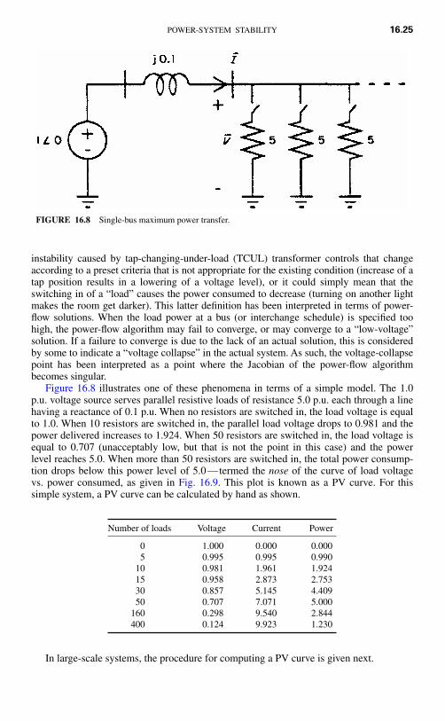
Voltage stability analysis of power systems means different things to different people. Itcan be loosely defined as the state of a power system when its voltage levels do notrespond in an expected manner when changes are made. This could mean a dynamic


instability caused by tap-changing-under-load (TCUL) transformer controls that changeaccording to a preset criteria that is not appropriate for the existing condition (increase of atap position results in a lowering of a voltage level), or it could simply mean that theswitching in of a “load” causes the power consumed to decrease (turning on another lightmakes the room get darker). This latter definition has been interpreted in terms of power-flow solutions. When the load power at a bus (or interchange schedule) is specified toohigh, the power-flow algorithm may fail to converge, or may converge to a “low-voltage”solution. If a failure to converge is due to the lack of an actual solution, this is consideredby some to indicate a “voltage collapse” in the actual system. As such, the voltage-collapsepoint has been interpreted as a point where the Jacobian of the power-flow algorithmbecomes singular.

Figure 16.8 illustrates one of these phenomena in terms of a simple model. The 1.0p.u. voltage source serves parallel resistive loads of resistance 5.0 p.u. each through a linehaving a reactance of 0.1 p.u. When no resistors are switched in, the load voltage is equalto 1.0. When 10 resistors are switched in, the parallel load voltage drops to 0.981 and thepower delivered increases to 1.924. When 50 resistors are switched in, the load voltage isequal to 0.707 (unacceptably low, but that is not the point in this case) and the powerlevel reaches 5.0. When more than 50 resistors are switched in, the total power consump-tion drops below this power level of 5.0— termed the nose of the curve of load voltagevs. power consumed, as given in Fig. 16.9. This plot is known as a PV curve. For thissimple system, a PV curve can be calculated by hand as shown.

Number of loads Voltage Current Power

0 1.000 0.000 0.0005 0.995 0.995 0.990

10 0.981 1.961 1.92415 0.958 2.873 2.75330 0.857 5.145 4.40950 0.707 7.071 5.000

160 0.298 9.540 2.844400 0.124 9.923 1.230

In large-scale systems, the procedure for computing a PV curve is given next.

FIGURE 16.8 Single-bus maximum power transfer.



1. Specify a Base-Case Condition

The base-case condition is normally some future scenario with forecasted loads and/ortransactions. For this base-case condition, the network power-flow equations are solvedfor the network voltages.

2. Specify a Direction for Power Increase

This type of voltage stability analysis considers the increase of power in some direc-tion. This power could be total load, the load at a particular bus, or a wheeling transactionfrom one or more import locations to one or more export locations. This power levelincrease will make up the horizontal axis of the PV curve.

3. Increment the Power Increase and Solve for System Voltages

Using power-flow analysis, the power level is increased by some amount and thepower flow is solved for the new system condition. If the power flow fails to solve, the in-crease is reduced until convergence is reached. If the power flow solves, the power levelis increased further and the power flow is solved again. This process is repeated until thenose of the PV curve is reached. Any bus voltage of interest may be plotted on the verti-cal axis against the power level on the horizontal. When the power-flow solution gets nearthe nose of the PV curve, the convergence may become a problem due to the ill-conditioning of the Jacobian matrix.

Related Calculations. The “continuation power flow” was created to solve the problemsof ill-conditioned power-flow Jacobian matrices near the nose of the PV curve. This typeof power flow uses more robust solution techniques that actually allow the precise deter-mination of the nose and the lower half of the PV curve.

FIGURE 16.9 PV curve.


DATA PREPARATION FOR LARGE-SCALEDYNAMIC SIMULATION

The North American interconnected power system network is probably the largest net-work of interconnected systems whose dynamic performance is routinely simulated underpostulated disturbances. The generating units, transmission elements, and loads compris-ing this network are owned and operated by hundreds of utility companies and millions ofcustomers. Because they are interconnected, the consequences of a disturbance on onesystem may be felt across ownership and regulatory boundaries, affecting the operation ofinterconnected systems. Advances in modeling of system elements can be fully exploitedonly if the parameters of those models can be efficiently obtained for a study. To achievethis, in November 1994, the North American Electric Reliability Council (NERC) createdthe System Dynamics Database Working Group to develop and maintain an integratedsystem dynamics database and associated dynamics simulation cases for the EasternInterconnection. This database is maintained in the Microsoft Access® database format.Similar databases have been established by the Electric Reliability Council of Texas(ERCOT) and the Western Systems Coordinating Council (WSCC), as these regions areelectrically isolated from the Eastern Interconnection, except for asynchronous (dc) ties.Preparation and submission of data to the appropriate database is now mandatory for allcontrol areas under NERC Planning Standard II.A.I, Measurement 4.

Data Requirements and Guidelines

The following requirements are taken from the NERC System Dynamics Database Work-ing Group Procedural Manual, dated October 5, 1999, “Appendix II: Dynamics DataSubmittal Requirements and Guidelines.” A current copy may be obtained from theNERC Web site, www.nerc.com. It should be noted that the data-submission format uti-lized is that of the PSS/E® program of Power Technologies, Inc., Schenectady, N.Y. Thelevel of modeling detail required may be considered as the current industry consensuseven in the absence of regulatory requirements. MMWG refers to the Multi-RegionalModeling Working Group, which annually prepares a series of power-flow cases repre-senting anticipated conditions at intervals over the planning horizon.

Requirements

I. Power Flow Modeling Requirements

1) All power flow generators, including synchronous condensers and SVCs, shallbe identified by a bus name and unit id. All other dynamic devices, such asswitched shunts, relays, and HVDC terminals, shall be identified by a bus nameand base kV field. The bus name shall consist of eight characters and shall beunique within the Eastern Interconnection. Any changes to these identifiers shallbe minimized.

2) Where the step-up transformer of a synchronous or induction generator or syn-chronous condenser is not represented as a transformer branch in the MMWGpower flow cases, the step-up transformer shall be represented in the power flowgenerator data record. Where the step-up transformer of the generator or con-denser is represented as a branch in the MMWG power flow cases, the step-uptransformer impedance data fields in the power flow generator data record shallbe zero and the tap ratio unity. The mode of step-up transformer representation,whether in the power flow or the generator data record, shall be consistent fromyear to year.


3) Where the step-up transformer of a generator, condenser, or other dynamic deviceis represented in the power flow generator data record, the resistance and reactanceshall be given in per unit on the generator or dynamic device nameplate MVA. Thetap ratio shall reflect the actual step-up transformer turns ratio considering the basekV of each winding and the base kV of the generator, condenser or dynamic de-vice.

4) In accordance with PTI PSSE requirements, the Xsource value in the power flowgenerator data record shall be as follows:

a) Xsource � X� di for detailed synchronous machine modelingb) Xsource � X� di for non-detailed synchronous machine modelingc) Xsource � 1.0 p.u. or larger for all other devices

II. Dynamic Modeling Requirements

1) All synchronous generator and synchronous condenser modeling and associateddata shall be detailed except as permitted below. Detailed generator models con-sist of at least two d-axis and one q-axis equivalent circuits. The PTI PSSE dy-namic model types classified as detailed are GENROU, GENSAL, GENROE,GENSAE, and GENDCO.The use of non-detailed synchronous generator or condenser modeling shall bepermitted for units with nameplate ratings less than or equal to 50 MVA underthe following circumstances:

a) Detailed data is not available because manufacturer no longer in business.b) Detailed data is not available because unit is older than 1970.

The use of non-detailed synchronous generator or condenser modeling shall alsobe permitted for units of any nameplate rating under the following circumstancesonly:

c) Unit is a phantom or undesignated unit in a future year MMWG case.d) Unit is on standby or mothballed and not carrying load in MMWG cases.

The non-detailed PTI PSSE model types are GENCLS and GENTRA. Whencomplete detailed data are not available, and the above circumstances do not ap-ply, typical detailed data shall be used to the extent necessary to provide com-plete detailed modeling.

2) All synchronous generator and condensers modeled in detail per RequirementII.A shall also include representations of the excitation system, turbine-governor,power system stabilizer, and reactive line drop compensating circuitry. The fol-lowing exceptions apply:

a) Excitation system representation shall be omitted if unit is operated undermanual excitation control.

b) Turbine-governor representation shall be omitted for units that do not regulatefrequency such as base load nuclear units and synchronous condensers.

c) Power system stabilizer representation shall be omitted for units where suchdevice is not installed or not in continuous operation.

d) Representation of reactive line drop compensation shall be omitted wheresuch device is not installed or not in continuous operation.

3) All other types of generating units and dynamic devices including induction gen-erators, static var controls (SVC), high-voltage direct current (HVDC) system,


and static compensators (STATCOM), shall be represented by the appropriatePTI PSSE dynamic model(s).

4) Standard PTI PSSE dynamic models shall be used for the representation of allgenerating units and other dynamic devices unless both of the following condi-tions apply:

a) The specific performance features of the user-defined modeling are necessaryfor proper representation and simulation of inter-regional dynamics, and

b) The specific performance features of the dynamic device being modeled can-not be adequately approximated by standard PSSE dynamic models.

5) Netting of small generating units, synchronous condensers or dynamic deviceswith bus load shall be permitted only when the unit or device nameplate rating isless than or equal to 20 MVA. (Note: any unit or device which is already nettedwith bus load in the MMWG cases need not be represented by a dynamic model.)

6) Lumping of similar or identical generating units at the same plant shall be per-mitted only when the nameplate ratings of the units being lumped are less than orequal to 50 MVA. A lumped unit shall not exceed 300 MVA. Such lumping shallbe consistent from year to year.

7) Where per unit data is required by a dynamic model, all such data shall be pro-vided in per unit on the generator or device nameplate MVA rating as given in thepower flow generator data record. This requirement also applies to excitation sys-tem and turbine-governor models, the per unit data of which shall be provided onthe nameplate MVA of the associated generator.

III. Dynamics Data Validation Requirements

1) All dynamics modeling data shall be screened according to the SDDB datascreening checks.

All data items not passing these screening tests shall be resolved with the genera-tor or dynamic device owner and corrected.

2) All regional data submittals to the SDDWG coordinator shall have previously un-dergone satisfactory initialization and 20 second no-disturbance simulationchecks for each dynamics case to be developed. The procedures outlined in Sec-tion III.H* of this manual (*yet to be written) may be applied for this purpose.

Guidelines

1) Dynamics data submittals containing typical data should include documentation, whichidentifies those models containing typical data. When typical data is provided for existingdevices, the additional documentation should give the equipment manufacturer, nameplateMVA and kV, and unit type (coal, nuclear, combustion turbine, hydro, etc.).

2) When user-defined modeling is used in the SDDWG cases, written justification shall besupplied explaining the dynamic device performance characteristics that necessitate use ofa user-defined model. The justifications for all SDDWG user-defined modeling shall beposted on the SDDWG Internet site as a separate document. (Note: Guideline 2 aboveshall become a requirement in January 2001 and thereafter.)

3) The voltage dependency of loads should be represented as a mixture of constant imped-ance, constant current, and constant power components (referred to as the ZIP model).The Regions should provide parameters for representing loads via the PTI PSSE CONLactivity. These parameters may be specified by area, zone, or bus. Other types of loadmodeling should be provided to SDDWG when it becomes evident that accurate represen-tation of interregional dynamic performance requires it.


MODEL VALIDATION

The response of excitation systems and governors, like other control systems, to achange in set point should be rapid but well damped. A modest overshoot of the intendedfinal output may be acceptable if it permits more rapid attainment of the target, but sus-tained or poorly damped oscillations are not. A technique that has been applied to suchmodels is to consider the exciter or governor isolated from the unit and the rest of thepower system and simulate variation of the field voltage or mechanical torque in re-sponse to step change in set point.

An excitation system model is validated by simulating its response for a two-to-five-sinterval following an increase in its voltage set point of perhaps 5 percent of the nominalvalue (e.g., from 1.0 to 1.05 p.u.). Governor models are similarly validated by simulatinga change in the desired power input, but governor response tests must be run for a consid-erably longer time, particularly for reheat units, as discussed above.

In making such simulations it is important that both initial and final output values bewithin applicable limits VRmax, VRmin, Pmax, and Pmin.

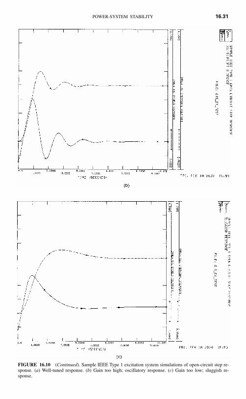
Figure 16.10 shows responses from a well-tuned IEEE Type 1 excitation system modeland two with different parameter values that are not well tuned. For comparison, the responseof IEEE Type 3 (GE SCPT) and IEEE Type 4 (noncontinuous regulator) excitation systemsare also shown in Fig. 16.11. The latter have not been installed in recent years but are stillfound on older machines. These have a rapid and a slow responding mechanism in parallelcontrolling the dc exciter, hence the name noncontinuous. The rapid-responding mechanismhas a significant dead band, typically 2 or 3 percent of nominal voltage, in its response.

FIGURE 16.10 Sample IEEE Type 1 excitation system simulations of open-circuit step response.(a) Well-tuned response. (b) Gain too high; oscillatory response. (c) Gain too low; sluggish response.


FIGURE 16.10 (Continued). Sample IEEE Type 1 excitation system simulations of open-circuit step re-sponse. (a) Well-tuned response. (b) Gain too high; oscillatory response. (c) Gain too low; sluggish re-sponse.


FIGURE 16.11 IEEE Type 3 (SCPT) and IEEE Type 4 (noncontinuous) excitation system simulations ofopen-circuit step response.


FIGURE 16.12 Governor response simulations. (a) Steam turbine units. (b) Hydro unit.


Figure 16.12a shows governor responses to a 10 percent change in load set point froma reheat (tandem compound) steam turbine. (Response of a nonreheat steam turbine issimilar.) Figure 16.12b shows the governor response of a hydro unit. Note that an initialreduction in power output from an increased valve setting is typical, due to the inertia ofthe water flowing through the penstock. When the gate valve is opened some, the head isinitially used to accelerate the water column and the head available at the turbine to gen-erate power is reduced.

BIBLIOGRAPHY

Anderson, Paul M., and Aziz A. Fouad. 1994. Power System Stability and Control (Revised Print-ing). New York: IEEE Press.

Bergen, Arthur R., and Vijay Vittal. 2000. Power System Analysis. Upper Saddle River, N.J.: PrenticeHall.

Byerly, Richard T., and Edward W. Kimbark. 1974. Stability of Large Electric Power Systems. NewYork: IEEE Press.

Elgerd, Olle I. 1982. Electric Energy Systems Theory: An Introduction. New York: McGraw-Hill.

Energy Development and Power Generating Committee of the Power Engineering Society. 1992.IEEE Standard 421.5-1992, IEEE Recommended Practice for Excitation System Models for PowerSystem Stability Studies. New York: Institute of Electrical and Electronics Engineers, Inc.

Kundur, Prabha. 1994. Power System and Stability and Control. New York: McGraw-Hill.

Machowski, Jan, Janusz Bialek, and James R. Bumby. 1997. Power System Dynamics and Stability.Chichester, U.K.: Wiley.

Pai, M. A. 1981. Power System Stability—Analysis by the Direct Method of Lyapunov. New York:North Holland.

Power System Engineering and Electric Machinery Committees of the IEEE Power Engineering So-ciety. 1991. IEEE Standard 1110-1991, IEEE Guide for Synchronous Generator Modeling Prac-tices in Stability Analyses. New York: Institute of Electrical and Electronics Engineers, Inc.

Sauer, Peter W., and M. A. Pai. 1998. Power System Dynamics and Stability. Upper Saddle River,N.J.: Prentice Hall.

Taylor, Carson W. 1994. Power System Voltage Stability. New York: McGraw-Hill.

Documents

SECTION 16 POWER-SYSTEM STABILITY - WordPress.comMay 16, 2011 · Power-system stability calculations fall into three major categories: transient, steady-state, and voltage stability