106

SECONDARY SCHOOL STUDENTS’ REASONING ABOUT CONDITIONAL PROBABILITY, SAMPLES, AND SAMPLING

PROCEDURES1

THEODOSIA PRODROMOU University of New England

theodosia.prodromou@une.edu.au

ABSTRACT In the Australian mathematics curriculum, Year 12 students (aged 16-17) are asked to solve conditional probability problems that involve the representation of the problem situation with two-way tables or three-dimensional diagrams and consider sampling procedures that result in different correct answers. In a small exploratory study, we investigate three Year 12 students’ conceptions and reasoning about conditional probability, samples, and sampling procedures. Through interviews with the students, supported by analysis of their work investigating probabilities using tabular representations, we investigate the ways in which these students perceive, express, and answer conditional probability questions from statistics, and also how they reason about the importance of taking into account what is being sampled and how it is being sampled. We report on insights gained about these students’ reasoning with different conditional probability problems, including how they interpret, analyse, solve, and communicate problems of conditional probability. Keywords: Statistics education research; Conditional probability; Samples;

Sampling; Learning probability; Statistics

1. INTRODUCTION Recent curricula of school mathematics (e.g., Australian Curriculum, Assessment,

and Reporting Authority [ACARA], 2016) advocate the broadening of probability and statistics in the school curriculum. Conditional probability is considered an integral part of the statistical literacy program of study in schools and at the tertiary education level (Tarr & Jones, 1997; Watson & Kelly, 2007). In the Australian curriculum, conditional probability is introduced at year 10 and it generally focuses on placing emphasis on conceptual understanding of the concept and calculating conditional probabilities, since the notion of conditional probability is a basic tool of probability theory (Feller, 1973, p. 114). Watson (1995) advocated that conditional probability and independence would be better to be taught in middle school mathematics in an intuitive manner. Several other researchers (e.g., Jones, Langrall, Thornton, & Mogill, 1999; Tarr, 2002; Tarr & Jones, 1997) pointed out that conditional probability and independence need not be deferred until middle school students have developed robust skills in comparing fractions.

In the Australian curriculum (ACARA, 2016), conditional probability is typically introduced by random experiments involving sampling both “with” and “without” replacement. Australian middle school students are expected to be able to: (1) list all outcomes for two- and three-step chance experiments, both with and without replacement, using organized lists, tables or tree diagrams or arrays, and (2) assign Statistics Education Research Journal, 15(2), 106-125, http://iase-web.org/Publications.php?p=SERJ © International Association for Statistical Education (IASE/ISI), November, 2016

107

probabilities to outcomes and determine probabilities for events. According to the New South Wales Syllabus (New South Wales Board of Studies, 2012) students at Year 10 are also required to “calculate probabilities of events where a condition is given that restricts the sample space”, and “critically evaluate conditional statements used in descriptions of chance situations” (Stage 5.2) especially with reference to understanding and explaining dependent and independent events or identifying and explaining common misconceptions related to chance experiments.

In this practical investigation of students’ reasoning about conditional probability, we focus on students’ reasoning when engaged in solving a puzzle known as the Two Children problem. The process of having students resolving the puzzle, which can be viewed as a paradox, helps them to develop “crucial properties of the theory involved” (Borovcnik & Kapadia, 2014, p. 35) about conditional probability in situations where the current concept yields a solution, “that seems intuitively unacceptable” (Borovcnik & Kapadia, p. 35).

2. THEORETICAL FRAMEWORK

Research studies have shown that school students reason about conditional probability using a variety of strategies to make conditional probability judgements with or without using fractions or numerical probabilities (e.g., Fischbein & Gazit, 1984; Jones et al., 1997; Tarr & Lannin, 2005; Watson & Moritz, 2002). Fischbein and Gazit (1984) attempted to capture 285 students’ (grades 5-7) probabilistic thinking in conditional probability when engaged in tasks required to determine conditional probabilities in with- and without-replacement situations. They found out that the percentage of students who correctly determine conditional probabilities in without-replacement situations was generally lower than the percentage of students who correctly determine conditional probability in with replacement tasks. It is noteworthy to point out that approximately 24% of fifth graders correctly determined conditional probabilities in both with- and without-replacement tasks. Moreover, 63% of the sixth grade students correctly responded to questions about with-replacement tasks, and 43% of the sixth grade students correctly responded to questions about without-replacement tasks. The percentage of the seventh graders who provided correct responses to with-replacement tasks was 89% and 71% percent to without-replacement tasks.

Fischbein and Gazit (1984) identified and explained two common misconceptions related to students’ thinking about conditional probability. According to Fischbein and Gazit in a without-replacement situation: (a) students struggled to realise that the sample space had changed and (b) students’ probability judgments of an event were impaired by comparing the number of favourable outcomes for the event before and after the first trial rather than by considering it in relation to the total number of outcomes (pp. 8-9).

Another study reported that students who engaged in conditional probability judgments, were impaired by misusing the phrase “50-50 chance” in probability situations where the sample space contained two elements. In such situations, students often assumed that each outcome had a 50-50 chance even when the two outcomes in the space were not equally likely to occur (Tarr, 2002).

The phrase 50-50 chance was also used in probability situations when the sample space contained an equal number of more than two elements, and concluded that each event had a 50-50 chance of occurring. Both of these uses of the phrase 50-50 chance were problematic because students’ probabilistic reasoning was in terms of probabilities in without-replacement situations. When students dealt with without-replacement tasks, persistent use of the phrase 50-50 chance prevented students from recognizing that the

108

conditional probabilities of all events changed in without-replacement situations due to the change caused by the conditioning event.

Research literature clearly suggests that the main objective of instruction is to help students develop the idea that the sample space is changed in without-replacement tasks (Borovcnik & Bentz, 1991; Falk, 1983; Falk, 1988; Tversky & Kahneman, 1982; Watson, 2005; Watson & Moritz, 2002). It is of paramount importance to help students study the composition of the sample space in relation to the total number of outcomes after sampling without replacement and take into account the change of the modified sample space due the conditioning event. For example, when we have a container that contained 8 red balls and we drew 2 red balls without replacing them, then there are only 6 red balls left. Not only does the number of one color of ball change in sampling without replacement (in this example, the number of red balls changes), but also the entire sample space has been modified by the change in the number of one of the possible outcomes, even if the number of non-red balls has remained constant.

Additionally, students’ understanding of the role of “sample space” helps them to monitor the composition of the sample space, make probability comparisons, and determine that the probability of all events change in non-replacement situations (Tarr & Lannin, 2005, p. 231). Hence, understanding the role of the sample space is a key factor in making conditional probability judgements.

Hays (2014) pointed out that “imbedded with difficulties in understanding probability are students’ difficulties with proportional reasoning” (p. 2). These difficulties in proportional reasoning have an ongoing negative impact on students’ statistical literacy because proportional reasoning permeates much of the reasoning associated with probability. At the core of the students’ comprehension of conditional probability is their understanding of proportional reasoning and their ability to conceptualise their answer as a fraction, or decimal, or percentage, or ratio between a specific condition of interest and the total number of outcomes of a sample space.

Jones et al. (1997) formulated a cognitive framework that captures the manifold nature of middle school students’ (9-13 year olds) probabilistic reasoning and understanding of conditional probability and statistical independence. In it, they suggested four levels of thinking with respect the conditional probability. Level 1 is associated with subjective thinking. Children at this level tend to rely on subjective judgments, ignoring any numerical information in formulating any conditional probability statements. Additionally, these Level 1 children might struggle to list all the outcomes in with- and without-replacement tasks and their judgements are made without regard to the changing probability of any event in a without-replacement task.

Children exhibiting Level 2 thinking (transitional) begin to gain awareness of the changing conditional probabilities of some events in without-replacement tasks but their judgements are still limited to the occurrence of preceding events.

Students at Level 3 (Informal Quantitative) are able to list the complete set of outcomes in a with- or without-replacement task. These students appreciate the role that quantities play in the sample when making conditional probability judgments. In particular, students exhibiting Level 3 thinking recognise that the probabilities of all events changed in a without-replacement task and began to use ratios or relative frequencies to determine conditional probabilities.

Students at Level 4 (Numerical) can assign numerical values, ratios rather than fractions, to the changing conditional probabilities when interpreting probabilities in without-replacement situations. Even when students’ progress towards the Numerical Level, difficulties remain (Tarr & Lannin, 2005). This article considers an alternative perspective in which conditional probabilistic thinking is used in resolving a paradox.

109

Probability is especially rich in puzzles and paradoxes, which can serve as triggers for great conceptual change.

Borovcnik and Kapadia (2014) discuss the role of paradox in mathematical education: Progress in the development of mathematical concepts is accompanied by controversies, ruptures, and new beginnings. The struggle for truth reveals interesting breaks highlighted by paradoxes and mark a situation, which reflects a contradiction to the current base of knowledge. Yet, there is an opportunity to renew the basis and proceed to wider concepts, which can embrace and dissolve the paradox. (p. 35) A paradox, in general, is a situation that yields a resolution that appears to be

intuitively unacceptable. Therefore a paradox demonstrates that the intuitive basis of the background ideas embedded in a paradox requires improvement or the target concept is in a clear opposition to the expectation of the solvers who deepen their knowledge from paradoxes, learning about critical properties of the theory involved. The paradoxes present challenging situations and can even lead experts to errors. Borovcnik and Kapadia (2014) argued that the target concepts can be better understood when learners engage with paradoxes than by engaging with a sequential exposition of mathematical theory and examples.

3. APPROACH AND AIM OF THE STUDY

According to Diaz and de la Fuente (2007), students’ difficulties might be overcome

if the concept of conditional probability is taught in conjunction with material on intuitive strategies and inferential errors so students are confronted with their misconceptions. In this research study the aim is to observe the conceptual struggle that needs to take place for Year 12 students to engage in conditional probability situations. To do so the author acknowledges a constructivist stance in which the Two Children problem (see Section 3.2) might effectively be used to highlight the crucial contradictions of the unitive basis of the concept of conditional probability. Yet, participants are provided with opportunities to use their current intuitions effectively as resources for the construction of new intuitions that are less apt to lead to subjective judgments and concepts, which are contrary to the expectation of the solver.

I begin by clarifying my perspective on what I consider as the two key factors that impact students’ conditional probability judgments.

These factors are: 1) the role of the sample space in determining the probability of an event; and 2) proportional reasoning.

Although two-way tables and tree diagrams are both effective representations for this kind of probability analysis, and we, as researchers, can learn from analysing patterns of student reasoning using either representation, in this article we focused on students who used two-way tables.

By focusing on conditional probability reasoning, in designing this study, I hypothesized that Year 12 students who engaged in conditional probability problems could perform probability analysis representing the problem situation with two-way tables or tree diagrams and computing probabilities by considering the total number of equally likely outcomes and that are favourable – including comparisons of the changing number of elements comprising the sample space – or alternatively by utilising the conditional probability formula P(A|B) = P(A∩B)

P(B). The aforementioned possible ways of

reasoning about a problem are not the only two ways that students will reason about such

110

problems. A large portion of the student body would use improper techniques to answer a conditional probability question. But those techniques are not the focus of this article.

Understanding the role of the changing number of elements comprising the sample space in assigning numerical probabilities to make conditional probability judgments is typically a characteristic of students at Level 3 (Informal Quantitative) and Level 4 (Numerical) of the framework of Jones, Langrall, Thornton, and Mogill (1997). In this study, although I do not make assumptions about the abilities of the participants, I do assume that the participating students have been introduced to techniques that allow them to answer the study questions correctly.

The aim of this study was to investigate Year 12 students’ reasoning about conditional probabilities. There were two specific aspects of interest:

1) How do students reason about conditional probabilities while they create two-way tables for illustrating the reduced sample spaces and the number of favourable outcomes of problems to represent the problem situations before the numerical calculation of conditional probabilities?

2) Do students have specific difficulties when making conditional probability judgements? If students have difficulties, what are those difficulties, and what variation is there amongst the difficulties faced by different students?

Information about these questions can potentially be used by teacher educators as a starting point for developing teaching materials for teaching conditional probability.

4. RESEARCH METHODS

4.1. PARADIGM

This research article reports on data gathered to gain information regarding students’

reasoning about conditional probability problems that involve the representation of the problem situation with two-way tables or three-dimensional diagrams, and examines how students consider sampling procedures that result in different correct answers. The data were gathered as part of a broader study on researching students’ probabilistic reasoning while studying the topic of probability in school mathematics (see Prodromou, 2013a; 2013b). The research study of students’ probabilistic reasoning while studying the topic of probability in school mathematics was organized around students’ reasoning about probabilistic concepts, calculation of probabilities, and reasoning about probability problem solving situations.

Our instructional goals were for the participants to be able to understand and work with conditional probability; specifically, to create tree diagrams or two-way tables for illustrating the reduced sample spaces and the number of favourable outcomes of problems, and then to perform numerical calculations of conditional probabilities. Hence, they should develop ways of thinking about conditional probability that depend on the use of diagrams (representations) or ways of thinking about diagrams that help to decide what kind of diagrams to use to deal with different kinds of problems.

Some tasks in the broader study were designed to elicit common student reasoning documented in the literature whereas others were added during the study as follow-up challenges to specific types of arguments displayed by the participating students.

The broader study included several tasks about conditional probability, such as those using examples of marbles, but in this article we focus on tasks involving a paradox and a puzzle and their variations. The rationale behind the creation of these variations was to obtain a collection of problems that are similar enough to each other to inspire students to

111

make connections between the types of reasoning used for each problem, but also different enough potentially to trigger a range of students’ arguments. 4.2. PROBLEMS

This research study’s questions were derived from the Two Children Problem

introduced by Martin Gardner (1959, 1961, 2006) and discussed in the literature by many authors (e.g., Juul, 2010; Khovanova, 2012; Marks & Smith, 2011; Rehmeyer, 2010; Taylor & Stacey, 2014). The first two questions are Gardner’s:

1. Problem 1: Mr. Jones has two children. The older child is a boy. What is the probability that both children are boys? (The original problem was about girls, though we have changed to boys to allow for consistency within the presentation of the various problems discussed in the paper.)

2. Problem 2: Mr. Smith has two children. At least one of them is boy. What is the probability that both children are boys?

The rest of the questions were variations on these first two. The third question of this study comes from Puzzler Gary Foshee (Khovanova, 2012, p. 258) who presented the following problem at the Ninth “Gathering 4 Gardner” in 2000:

3. Problem 3: Mr Ng has two children. One is a boy born on a Tuesday. What is the probability that both children are boys? (The “Tuesday Birthday Problem” is considered a paradox that attracts ongoing interest.)

Problems 4 and 5 are further variations of the original problems: 4. Problem 4: Mr. Taylor has two children and at least one is a boy born after

midday. What is the probability that both children are boys? 5. Problem 5: Mr. John has two children and at least one is a boy born in autumn.

What is the probability that both children are boys? Questions 6 and 7 are asked to investigate students’ understanding of conditional

probabilities, sampling procedures and sample spaces: 6. Consider that there are 19600 families who have two children standing in a sports

ground. We ask all who have one son to remain while all those who have two daughters leave. What is the probability to randomly choose a family who has two sons from those remaining on the sports ground?

7. Again, starting with 19600 families who have two children, we ask all families who have a son with a birthday on Tuesday to remain on the sports ground and all others leave. What is the [percentage/proportion] of families with two sons remaining on the spots ground? If we select a family at random from those who remain, what is the probability that the family chosen will have two sons?

4.3. PARTICIPANTS

The above problems were given to 15 Year 12 students during their engagement with

conditional probability problems that involve the representation of the problem situation with two-way tables or three-dimensional diagrams. The students studied at a rural secondary school in New South Wales in Australia. Out of the 15 students who were given the questions, 12 used two-way tables to get an answer, and three were randomly selected from this group. We worked only with three students at a time in order to be able to follow closely each student’s reasoning, both during each session and later during data

112

analysis. The three students, George, Chris, and Annie (all students’ names are pseudonyms) were interviewed separately by the author.

4.4. PROCEDURE

Following the students’ analysis of probabilities in their notebooks, George, Chris

and Annie were interviewed separately by the author and asked to explain in detail their reasoning on the seven questions/problems. Each interview was conducted after the students answered all the questions during the six problem sessions (Problem 6 and Problem 7 were solved during one problem session) lasting approximately 30-60 minutes each, during which they progressed through the 7 problems at their own pace. Students were encouraged to provide justifications for their answers. At this stage, the interviewer neither validated the students’ solutions nor attempted to steer their reasoning in a particular direction. These problem sessions were videotaped. When the three students completed the 7 individual questions/problems, they met and were encouraged to discuss the questions/problems and provide justifications for their answers. This discussion lasted for 2 hours and was also videotaped.

4.5. ANALYSIS

The problem-solving sessions, totaling 5 hours and 30 minutes of video, and a

discussion session taking 2 hours of video, were transcribed. These transcripts were analysed according to the approach of progressive focusing (Robson, 1993). This approach enabled a narrower field of focus to be established, selecting out significant features for future focus regarding the reasoning that students used to justify their approach to solve the problems, how this reasoning altered over time, and how the representation of the situation with two-way tables induced shifts in their reasoning. I noted that shifts in reasoning occurred when the participants compared their reasoning for the problem they were currently solving to the problems that they had previously encountered and drew connections amongst the sample space of the different problems and considered the number of equally likely outcomes in total before computing the conditional probabilities. Subsequently, we focused on the ways in which students made comparisons amongst the two-way tables for illustrating the sample spaces of the problems in their reasoning and how this process contributed to their reasoning.

5. RESULTS

We start with a two-way table that students created to analyse Problem 2 (Figure 1),

and then continue to a closer analysis of their reasoning about Problem 3, in which they relied on the table made in Problem 2 to create a new table.

113

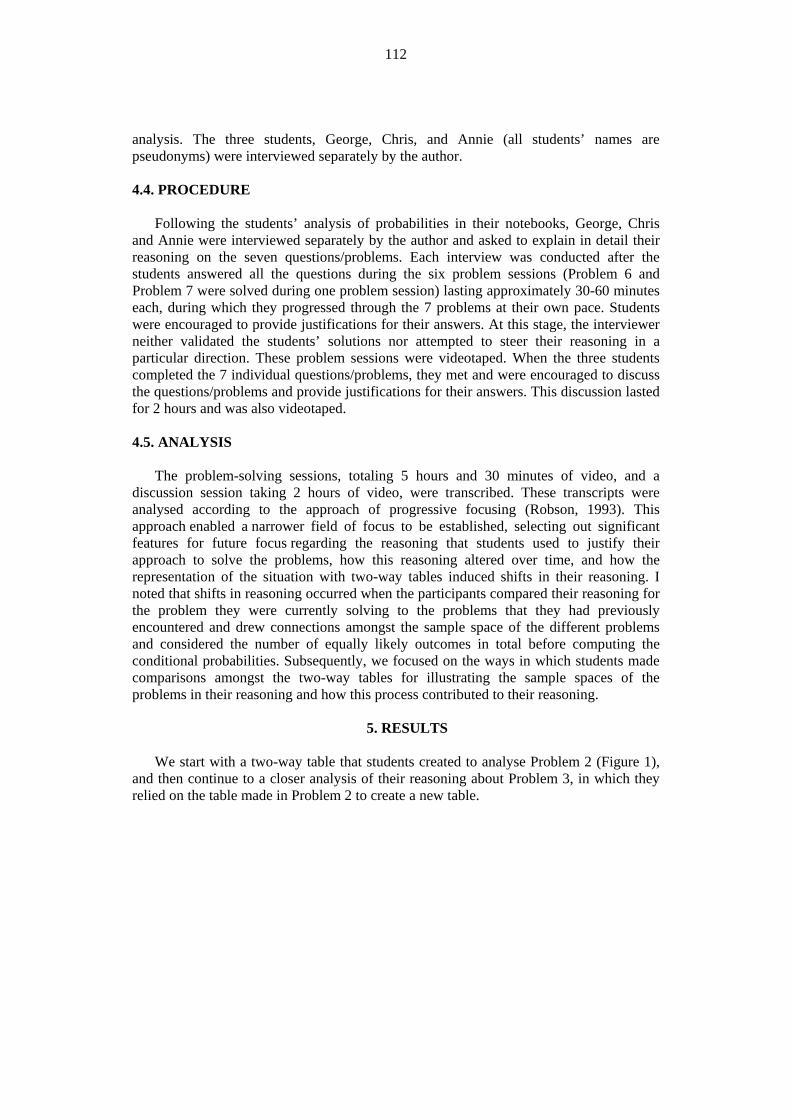
Figure 1. Represent the Problem 2 situation with a two-way table.

Discuss Problem 3 and compare Problem 3 to Problems 1-2 When students

attempted to solve Problem 3, they noted that Problem 3 seemed the same as Problem 2. We present two instances of this type of reasoning:

George: What has the day of the week on which one of the boys is born has anything to do with the sex of her sibling?... So the answer must be 1

3… However, Foshee ’s

answer was 1327

… Similarly, Annie wrote:

Annie: When I first looked at Problem 3, it seemed exactly the same as Problem 2, so the answer was expected to be 1

3… Knowing that Foshee’s answer was 13

27… I started

thinking to analyse the impact of the condition “born on a Tuesday” because such a condition seemed to increase the probability that the other sibling is a boy from 1

3 for

the Problem 2, through Foshee’s example for 1327

for Problem 3 and up to the 12 for

Problem 1…but when Mr. Jones has two children and the older child is a boy. The probability that both children are boys is 1

4 .

The students focused on the probability still being more than the expected 1 3

that in

turn is more than the probability of 14 of having two boys on a two child family.

Making assumptions about birthdays The students made assumptions about the

likelihood of birthdays. Chris: First we assume that boys and girls are equally likely to be born, so the

probability that a baby is a boy is one half (also a girl). … Chris: At this stage, I assumed that the girls and boys are equally likely to be born, so the

probability that a baby is a boy is one half (also a girl). I also assumed that the sex of one child in the family does not affect the sex of children to be born.

Annie: I agree. Assumptions of these types have already been documented in the literature in the

content of similar problems (e.g., Rodgers & Doughty, 2001) and the 50/50 assumption was also embedded in stating that the answer to Problem 2 is 1

3. Hence, participants’

114

reactions to these problems did not come as a surprise. However, the problems used in our research led to instances of student reasoning relying on similar assumptions about the time of birth of a child, as seen in the following utterances:

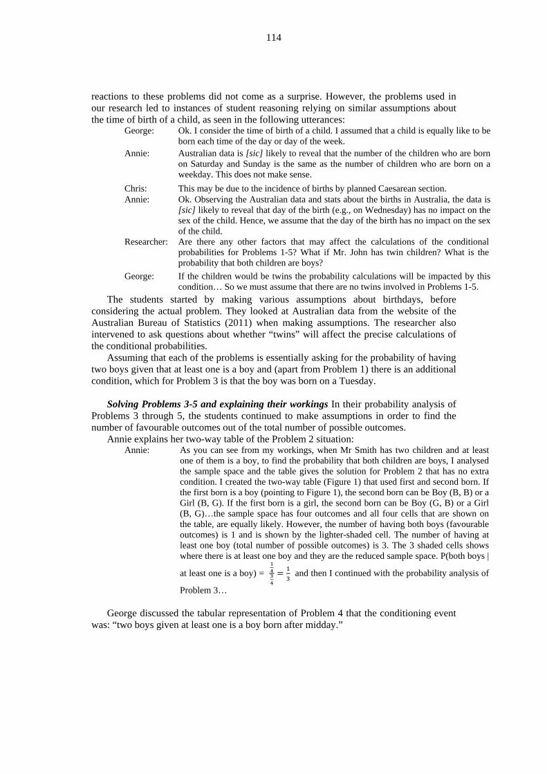
George: Ok. I consider the time of birth of a child. I assumed that a child is equally like to be born each time of the day or day of the week.

Annie: Australian data is [sic] likely to reveal that the number of the children who are born on Saturday and Sunday is the same as the number of children who are born on a weekday. This does not make sense.

Chris: This may be due to the incidence of births by planned Caesarean section. Annie: Ok. Observing the Australian data and stats about the births in Australia, the data is

[sic] likely to reveal that day of the birth (e.g., on Wednesday) has no impact on the sex of the child. Hence, we assume that the day of the birth has no impact on the sex of the child.

Researcher: Are there any other factors that may affect the calculations of the conditional probabilities for Problems 1-5? What if Mr. John has twin children? What is the probability that both children are boys?

George: If the children would be twins the probability calculations will be impacted by this condition… So we must assume that there are no twins involved in Problems 1-5.

The students started by making various assumptions about birthdays, before considering the actual problem. They looked at Australian data from the website of the Australian Bureau of Statistics (2011) when making assumptions. The researcher also intervened to ask questions about whether “twins” will affect the precise calculations of the conditional probabilities.

Assuming that each of the problems is essentially asking for the probability of having two boys given that at least one is a boy and (apart from Problem 1) there is an additional condition, which for Problem 3 is that the boy was born on a Tuesday.

Solving Problems 3-5 and explaining their workings In their probability analysis of

Problems 3 through 5, the students continued to make assumptions in order to find the number of favourable outcomes out of the total number of possible outcomes.

Annie explains her two-way table of the Problem 2 situation: Annie: As you can see from my workings, when Mr Smith has two children and at least

one of them is a boy, to find the probability that both children are boys, I analysed the sample space and the table gives the solution for Problem 2 that has no extra condition. I created the two-way table (Figure 1) that used first and second born. If the first born is a boy (pointing to Figure 1), the second born can be Boy (B, B) or a Girl (B, G). If the first born is a girl, the second born can be Boy (G, B) or a Girl (B, G)…the sample space has four outcomes and all four cells that are shown on the table, are equally likely. However, the number of having both boys (favourable outcomes) is 1 and is shown by the lighter-shaded cell. The number of having at least one boy (total number of possible outcomes) is 3. The 3 shaded cells shows where there is at least one boy and they are the reduced sample space. P(both boys |

at least one is a boy) = 1434

= 13 and then I continued with the probability analysis of

Problem 3…

George discussed the tabular representation of Problem 4 that the conditioning event was: “two boys given at least one is a boy born after midday.”

115

George: I found the condition of Problem 4 less complicated compared to Problem 3, so I analysed the Problem 4 that was asking that “two boys given at least one is a boy born after midday”. I defined BAm (a boy born in the morning), BPm (a boy born in the afternoon), GAm (a girl born in the morning), GPm (a girl born in the afternoon). I then defined the sample space (BAm, BPm), (BAm, GPm), (BAm, GAm), (BPm, GAm)…..) that has 16 outcomes (Figure 2). The total number of favourable outcomes to have two boys is 3, and the number of outcomes indicating that at least one boy was born after midday is 7. We have seven shaded squares that is the intersection of the horizontal shading of the row BPm and the vertical shading of the column BPm. The intersection of the horizontal and vertical shading, occurs because it does not specify which child was born after midday. That intersection of the horizontal and vertical shading, pointing to Figure 2, shows the number of favourable outcomes. Thus P(both boys | at least one boy born after midday) =

316716

= 37 .

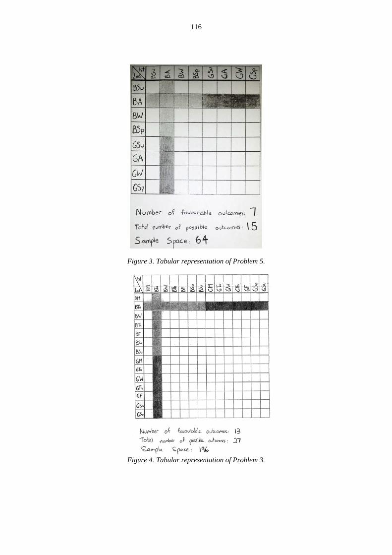
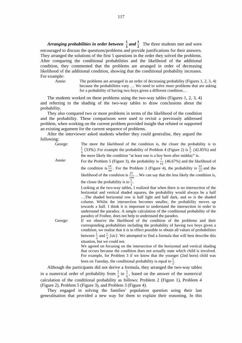
Chris: Let me explain Problem 5 and solving Problem 5 (Figure 3) in the same manner, based on Problem 4 that has as a condition “two boys given at least one is a boy born in autumn”. We define as we did in Problem 4, BSu to indicate a boy born in summer, and BA to indicate a boy born in autumn, BW to indicate a boy born in winter, BSp to indicate a boy born in spring, etc. (Figure 3) The outcomes of the sample space is 64 and the number of favourable outcomes is 7, whereas the total number of at least one is a boy born in autumn, is 15, and

P(both boys | at least one boy born in autumn) = 7641564

= 715

.

The participants reason about these three examples using two-way tables (see Figures 1, 2, 3) to analyse the sample space and the favourable outcomes. Annie and George reasoned about the horizontal and vertical shading of the two-way tables that shows the number of possible outcomes and the intersection of the horizontal and vertical shading that shows the number of favourable outcomes.

Figure 2. Tabular representation of Problem 4.

116

Figure 3. Tabular representation of Problem 5.

Figure 4. Tabular representation of Problem 3.

117

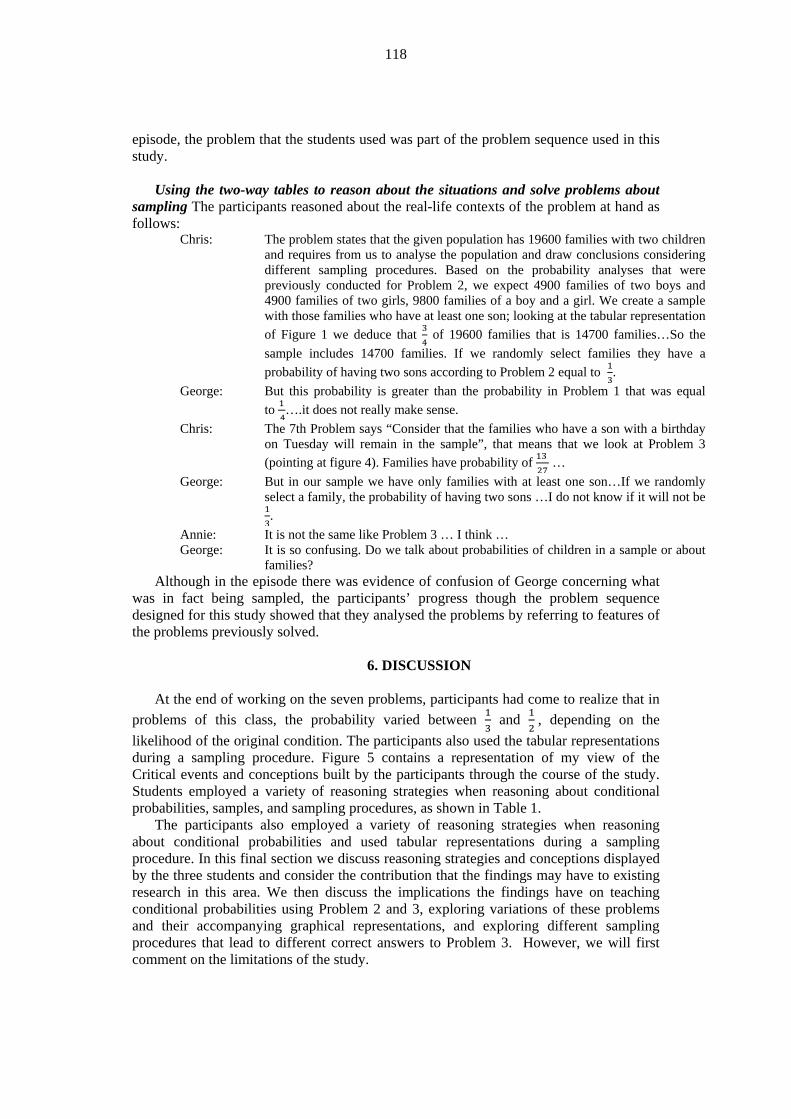
Arranging probabilities in order between 𝟏𝟏𝟑𝟑 and 𝟏𝟏

𝟐𝟐 The three students met and were

encouraged to discuss the questions/problems and provide justifications for their answers. They arranged the solutions of the first 5 questions in the order they solved the problems. After comparing the conditional probabilities and the likelihood of the additional condition, they commented that the problems are arranged in order of decreasing likelihood of the additional condition, showing that the conditional probability increases. For example:

Annie: The problems are arranged in an order of decreasing probability (Figures 1, 2, 3, 4) because the probabilities vary … We need to solve more problems that are asking for a probability of having two boys given a different condition…

The students worked on these problems using the two-way tables (Figures 1, 2, 3, 4) and referring to the shading of the two-way tables to draw conclusions about the probability.

They also compared two or more problems in terms of the likelihood of the condition and the probability. These comparisons were used to revisit a previously addressed problem, when working on the current problem provided insight that refuted or supported an existing argument for the current sequence of problems.

After the interviewer asked students whether they could generalise, they argued the following:

George: The more the likelihood of the condition is, the closer the probability is to 13

(33%). For example the probability of Problem 4 (Figure 2) is 3 7

(42.85%) and the more likely the condition “at least one is a boy born after midday” is.

Annie: For the Problem 5 (Figure 3), the probability is 7 15

(46.67%) and the likelihood of

the condition is 15 64

. For the Problem 3 (Figure 4), the probability is 13 27

and the

likelihood of the condition is 27 196

. .. We can say that the less likely the condition is,

the closer the probability is to 1 2.

Looking at the two-way tables, I realized that when there is no intersection of the horizontal and vertical shaded squares, the probability would always be a half …The shaded horizontal row is half light and half dark, and so is the shaded column. Whilst the intersection becomes smaller, the probability moves up towards a half. I think it is important to understand the intersection in order to understand the paradox. A simple calculation of the conditional probability of the paradox of Foshee, does not help to understand the paradox.

George: If we observe the likelihood of the condition of the problems and their corresponding probabilities including the probability of having two boys given a condition, we realise that it is in effect possible to obtain all values of probabilities between 1

2 and 1

3 [sic]. We attempted to find a formula that will best describe this

situation, but we could not. We agreed on focusing on the intersection of the horizontal and vertical shading that occurs because the condition does not actually state which child is involved. For example, for Problem 3 if we know that the younger (2nd born) child was born on Tuesday, the conditional probability is equal to 1

2.

Although the participants did not derive a formula, they arranged the two-way tables in a numerical order of probability from 1

3 to 1

2 , based on the answer of the numerical

calculation of the conditional probability as follows: Problem 2 (Figure 1), Problem 4 (Figure 2), Problem 5 (Figure 3), and Problem 3 (Figure 4).

They engaged in solving the families’ population question using their last generalisation that provided a new way for them to explain their reasoning. In this

118

episode, the problem that the students used was part of the problem sequence used in this study.

Using the two-way tables to reason about the situations and solve problems about

sampling The participants reasoned about the real-life contexts of the problem at hand as follows:

Chris: The problem states that the given population has 19600 families with two children and requires from us to analyse the population and draw conclusions considering different sampling procedures. Based on the probability analyses that were previously conducted for Problem 2, we expect 4900 families of two boys and 4900 families of two girls, 9800 families of a boy and a girl. We create a sample with those families who have at least one son; looking at the tabular representation of Figure 1 we deduce that 3

4 of 19600 families that is 14700 families…So the

sample includes 14700 families. If we randomly select families they have a probability of having two sons according to Problem 2 equal to 1

3.

George: But this probability is greater than the probability in Problem 1 that was equal to 1

4….it does not really make sense.

Chris: The 7th Problem says “Consider that the families who have a son with a birthday on Tuesday will remain in the sample”, that means that we look at Problem 3 (pointing at figure 4). Families have probability of 13

27 …

George: But in our sample we have only families with at least one son…If we randomly select a family, the probability of having two sons …I do not know if it will not be 13.

Annie: It is not the same like Problem 3 … I think … George: It is so confusing. Do we talk about probabilities of children in a sample or about

families? Although in the episode there was evidence of confusion of George concerning what

was in fact being sampled, the participants’ progress though the problem sequence designed for this study showed that they analysed the problems by referring to features of the problems previously solved.

6. DISCUSSION

At the end of working on the seven problems, participants had come to realize that in

problems of this class, the probability varied between 13 and 1

2 , depending on the

likelihood of the original condition. The participants also used the tabular representations during a sampling procedure. Figure 5 contains a representation of my view of the Critical events and conceptions built by the participants through the course of the study. Students employed a variety of reasoning strategies when reasoning about conditional probabilities, samples, and sampling procedures, as shown in Table 1.

The participants also employed a variety of reasoning strategies when reasoning about conditional probabilities and used tabular representations during a sampling procedure. In this final section we discuss reasoning strategies and conceptions displayed by the three students and consider the contribution that the findings may have to existing research in this area. We then discuss the implications the findings have on teaching conditional probabilities using Problem 2 and 3, exploring variations of these problems and their accompanying graphical representations, and exploring different sampling procedures that lead to different correct answers to Problem 3. However, we will first comment on the limitations of the study.

119

Figure 5. Critical events and conceptions built by the participants through the course of

the study. 6.1. LIMITATIONS OF THE STUDY

This exploratory study was very small, focusing on only three students. Within the

constraints of the study, many potential areas for investigation were not possible. For example, it was not possible to explore in detail students’ understandings and biases

120

about sampling procedures that result in obtaining different correct answers to conditional probability problems.

6.2. CRITICAL EVENTS AND CONCEPTIONS BUILT BY THE PARTICIPANTS

Although acknowledging the limitations of the research study, the findings seem to

suggest that specific potential characterisations of participants’ conceptions are obvious (see Table 1). These conceptions based on participants’ workings and responses to the 7 questions, are discussed further.

Table 1. Summary of three students’ conceptions and reasoning about conditional

probability, samples and sampling procedures

Critical events Description Developing conceptions

Student Reasoning

Episode 1 Discuss problem 3, and Compare problem 3 to problem 1-2.

Students make various assumptions about birthdays, before considering the actual problem. Likelihoods are estimated and compared to 1

3

answer of Problem 2, and to the probability of 1

4 of having two

boys in a two child family (Problem 1).

Girls and boys are equally likely to be born. Factors that may affect the calculations of conditional probability, i.e., the impact of the condition “born on a Tuesday”.

Led to sensible use of own contextual knowledge to judge reasons that probability calculations may be impacted by a condition.

Episode 2 Making assumptions about birthdays.

Making assumptions (about birthdays, and sex). Students looked at Australian data from the website of the Australian bureau of statistics (2011) when making assumptions.

Equally likely to be born. Independent events: Two events, A and B, are independent if the fact that A occurs does not affect the probability of B occurring. Factors that may affect the calculations of the conditional probabilities: (e.g. the day of the birth has no impact on the sex of the child, but if the children would be twins the probability calculations will be impacted by this condition).

Explaining that: (1) Boys and girls are “equally likely to be born”, so the probability that a baby is a boy is one half (also a girl).” (2) The sex of one child in the family does not affect the sex of children to be born. Use of information provided by Australian data from the Australian Bureau of Statistics (2011) about the births in Australia. The data is likely to reveal that day of the birth (e.g., on Wednesday) has no impact on the sex of the child.

121

Episode 3 Solving problems 3-5 and explaining the workings.

The problem situation is shown with two-way tables (tabular representations) and use the two way tables to analyse the sample space, calculate the number of favourable outcomes out of the total number of possible outcomes, and reason about the situation.

Sample space. Number of equally likely outcomes, number of favourable outcomes, and number of possible outcomes. Conditioning event of conditional probability. Fractions, proportions (e.g. 42%).

Reasoning about the sample space (number of equally likely outcomes in total), by counting the number of shaded cells of the two-way table. Reasoning about the favourable outcomes referring to the shading to the lighter-shaded cell that is the intersection of the horizontal and vertical shading. Developing sense of associating the number of equally likely outcomes in total, the number of favourable outcomes, the number of possible outcomes, and the reduced sample space with conditional probability.

Episode 4 Arranging probabilities in order between 1

3

and 12 .

The problems are arranged in an order of decreasing probability. Students recognize that the problems have a range of probabilities between 13 and 1

2 .

Compare two or more problems in terms of the likelihood of the condition and value of the conditional probability.

The more the likelihood of the condition is, the closer the probability is to 13

(33%). The less likely the condition is, the closer the probability is to 1

2 (50%).

Comparing two or more problems in terms of the likelihood of the condition and the probability. Looking at the two-way tables, when there is no intersection of the horizontal and vertical shaded squares, the probability would always be a half … Whilst the intersection becomes smaller, the probability moves up towards a half. Focusing on the intersection of the horizontal and vertical shading that occurs because the condition does not actually state which child is involved.

Episode 5 Discussing samples Using the two-way tables to reason about the

Students analysed the population and drew conclusions considering different sampling procedures referring to

Create samples from sampling procedures and calculate the number of the elements of the samples based on information from

Reasoning and explaining their answers based on the probability analyses previously conducted for problems 1 and 2.

122

situations and solve problems about sampling.

probability analyses of the problems previously solved.

the two-way tables. Random selection of a sample (e.g., randomly select a family, with two sons).

Explaining that 9800 families of a boy and a girl (4900 families of two boys and 4900 families of two girls), and creating a sample with those families who have at least one son. Looking at the tabular representation of Problem 2, 3

4 of 19600

families is 14700. Students realised that if they randomly select families, the probability of having two sons according to Problem 2 is equal to 1

3.

Confusions about what was sampled and the sampling procedure.

6.3. IMPLICATIONS FOR TEACHING

This set of problems and their tabular representations seem to serve as triggers for

students’ conceptual change. Paradoxes make students want to think harder about mathematics and solving problems and variations, raising students’ interest to understand better the crucial properties of the probability theory involved.

The tabular representations of the probability analysis in the form of two-way tables are mainly useful for illustrating the reduced sample spaces that are the core of conditional probability. Students’ understanding of the intersection of the horizontal and vertical shading when the condition does not specify which child is involved (e.g., younger child) is the cornerstone to understanding the paradox. Two-way tables can be used in schools to analyse obscure and complex conditional probabilistic situations.

Students might be given Problem 2, Problem 3, and the variations included in this paper and then engaged with sampling procedures (e.g., for example Problems 6 and 7) that produce different correct answers to Problem 3. At this stage, it will be beneficial to be emphasised that the Problem 3 paradox partially occurs because the sampling procedure clarifies neither what is to be sampled nor the sampling procedure. In such instances, the participants attempted to find a solution, attributing different interpretations to the problem and taking a logical approach, thereby employing analysis of the particular sampling procedure to avoid the confusion of what is sampled and how it is sampled. This type of reasoning that students invoke is essential because this confusion also occurs in some school mathematics probability problems. Hence, it is of paramount importance that all probability calculations and conclusions from statistics take into consideration what is being sampled and how it is being sampled.

More advanced students may be engaged with arranging all answers of conditional probabilities between 1

3 and 1

2 and deducing an appropriate general formula. Such a

general formula together with the tabular representations of the two-way tables could also

123

be used as an alternative view point of limits and their association to the probability of a final condition.

With an awareness of the connections created by students in constructing conceptions and reason across tasks, we conjecture that students attending to problems and variations such as those in the study will experience questions that significantly influence their thinking about probability and statistics.

Our findings suggest that: the way the probability was analysed, representing the problem situations with two-way tables had a strong influence on the types of reasoning that students used. The tabular representations elicited normatively correct reasoning and building in students a conceptual understanding of the role of the “sample space” and the “conditional probability of an event” as key factors in making conditional probability judgements.

REFERENCES

Australian Bureau of Statistics. (2011). Births, Australia, 2011. Accessed 10 March 2015 from https://www.abs.gov.au/ausatas/abs@.nsf/mf/3301.0

Australian Curriculum, Assessment and Reporting Authority (ACARA). (2016). Australian curriculum: Mathematics. Accessed 11 February 2016 version 7.5 from http://www.australiancurriculum.edu.au/mathematics/curriculum/f-10?layout=1#level9

Borovcnik, M., & Bentz, H. J. (1991). Empirical research in understanding probability. In R. Kapadia & M. Borovcnik (Eds.), Chance encounters: Probability in education (pp. 73-105). Dorchrecht, The Netherlands: Kluer Academic Publishers.

Borovcnik, M., & Kapadia, R. (2014). From puzzles and paradoxes to concepts in probability. In E. J. Shernoff & B. Sriraman (Eds.), Probabilistic thinking: Presenting plural perspectives (pp. 35-73). New York, NY: Springer. doi: 10.1007/978-94-007-7155-0_3

Diaz, C., & de la Fuente, I. (2007). Assessing students’ difficulties with conditional probability and Bayesian reasoning. International Journal of Mathematical Education, 2(3), 128-148.

Falk, R. (1983). Children’s choice behavior in probabilistic situations. In D. R. Grey, P. Holmes, V. Barnett, & G. M. Constable (Eds.), Proceedings of the First International Conference on Teaching Statistics (pp. 714-716). Sheffield, UK: Teaching Statistics Trust.

Falk, R. (1988). Conditional probabilities: Insights and difficulties. In R. Davidson & J. Swift (Eds.), Proceedings of the Second International Conference on the Teaching of Statistics (ICOTS-2) (pp. 292-297). Victoria BC, Canada: University of Victoria. Retrieved October 18, 2016, from http://iase-web.org/documents/papers/icots2/Falk.pdf

Feller, W. (1973). An introduction to probability theory and its applications (Vol. 1). New York: Wiley.

Fischbein, E., & Gazit, A. (1984). Does the teaching of probability improve probabilistic intuitions? Educational Studies in Mathematics, 15(1), 1-24.

Gardner, M. (1959). The Scientific American book of mathematical puzzles & diversions. New York: Simon & Schuster.

Gardner, M. (1961). The second Scientific American book of mathematical puzzles and diversions. Chicago: University of Chicago Press.

Gardner, M. (2006). Aha! A two volume collection: Aha! Gotcha aha! Insights. Washington, DC: Mathematical Association of America.

124

Hays, I. (2014). Teaching probability: Using levels of dialogue and proportional reasoning. In K. Makar, B. deSousa, & R. Gould (Eds.), Sustainability in statistics education. Proceedings of the Ninth International Conference on Teaching Statistics (ICOTS9, July, 2014), Flagstaff, Arizona, USA. Voorburg, The Netherlands: International Association for Statistics Education and International Statistical Institute.

Jones, G. A., Langrall, C. W., Thornton, C. A., & Mogill, A. T. (1997). A framework for assessing and nurturing young children’s thinking in probability. Educational Studies in Mathematics, 32(2), 101-125.

Juul, J. (2010). The ludologist. Accessed 11 February 2016 from https://www.jesperjuul.net/ludologist/tuesday-changes-everything-a-mathematical-puzzle

Khovanova T. (2012). Martin Gardner’s mistake. In M. Henle & B. Hopkins (Eds.), Martin Gardner in the twenty-first century (pp. 257-262). Washington, DC: Mathematical Association of America.

Marks, S., & Smith, G. (2011). The two-child paradox reborn? Chance, 24(1), 54-59. New York, NY: Springer. doi: 10.1007/s00144-011-0010-0

New South Wales Board of Studies. (2012). New Mathematics K-10 Syllabuses for the Australian curriculum. Sydney, Australia: New South Wales Board of Studies. Available at http://syllabus.bos.sw.edu.au/mathematics

Prodromou, T. (2013). Informal inferential reasoning: Interval estimates of parameters. International Journal of Statistics and Probability, 2(2), 136-152. doi: 10.5539/ijsp.v2n2p136

Prodromou, T. (2013). Estimating parameters from samples: Shuttling between spheres. International Journal of Statistics and Probability, 2(1), 113-124. doi: 10.5539/ijsp.v2n1p113

Rehmeyer J. (2010). ScienceNews. Accessed 18 October 2016 from https://www.sciencenews.org/article/when-intuition-and-math-probably-look-wrong

Robson, C. (1993). Real World Research. Oxford: Blackwell. Rodgers, J.L., & Doughty, D. (2001). Does having boys run in the family? Chance, 14(4),

8-13. Tarr, J. E. (2002). The confounding effects of “50-50 chance” in making conditional

probability judgements. Focus on Learning Problems in Mathematics, 24(4), 35-53. Tarr, J. E., & Jones, G. A. (1997). A Framework for assessing middle school students’

thinking in conditional probability and independence. Mathematics Education Research Journal, 9(1), 39-59.

Tarr, J. E., & Lannin, J. K. (2005). How can teachers build notions of conditional probability and independence? In G. A. Jones (Ed.), Exploring probability in school: Challenges for teaching and learning (pp. 215-238). New York: Springer.

Taylor, W., & Stacey, K. (2014). Gardner’s two children problems and variations: Puzzles with conditional probability and sample spaces. The Australian Mathematics Teacher, 70(2), 13-18.

Tversky, A., & Kahneman, D. (1982). Causal schemas in judgments under uncertainty. In D. Kahneman, P. Slovic, & A. Tversky (Eds.), Judgment under uncertainty: Heuristics and biases (pp. 117-128). Cambridge, UK: Cambridge University Press.

Watson, J. (1995). Conditional probability: Its place in the mathematics curriculum. Mathematics Teacher, 88(1), 12-17.

Watson, J. (2005). The probabilistic reasoning of middle school students. In G. A. Jones (Ed.), Exploring probability in school: Challenges for teaching and learning (pp. 145-169). New York: Springer.

125

Watson, J., & Kelly, B. (2007). The development of conditional probability reasoning. International Journal of Mathematical Education in Science and Technology, 38(2), 213-235.

Watson, J. M., & Moritz, J. B. (2002). School students’ reasoning about conjunction and conditional events. International Journal of Mathematical Education in Science and Technology, 33(1), 59-84.

THEODOSIA PRODROMOU

University of New England Armidale, NSW 2351

Australia