Embed Size (px)
Citation preview

Secondary PM2.5 MERPs Demonstrations
Michael Moeller, Region 42019 EPA Regional/State/Local Modelers' Workshop
Seattle, WA
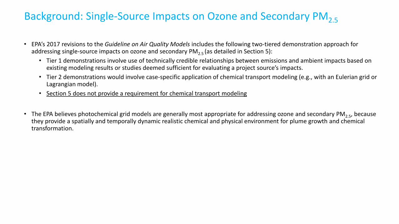
• EPA’s 2017 revisions to the Guideline on Air Quality Models includes the following two-tiered demonstration approach for addressing single-source impacts on ozone and secondary PM2.5 (as detailed in Section 5):
• Tier 1 demonstrations involve use of technically credible relationships between emissions and ambient impacts based on existing modeling results or studies deemed sufficient for evaluating a project source’s impacts.
• Tier 2 demonstrations would involve case-specific application of chemical transport modeling (e.g., with an Eulerian grid or Lagrangian model).
• Section 5 does not provide a requirement for chemical transport modeling
• The EPA believes photochemical grid models are generally most appropriate for addressing ozone and secondary PM2.5, because they provide a spatially and temporally dynamic realistic chemical and physical environment for plume growth and chemical transformation.
Background: Single-Source Impacts on Ozone and Secondary PM2.5

• April 30th 2019, the EPA released the final Guidance on the Development of Modeled Emission Rates for Precursors (MERPs) as a Tier 1 Demonstration Tool for Ozone and PM2.5 under the PSD Permitting Program or “MERPs Guidance”
• Update to the draft MERPs Guidance that was released in December 2016• Spreadsheet has also been posted to SCRAM that contains the underlying maximum impact and MERPs information (daily
PM2.5, annual PM2.5, and daily maximum 8-hr average O3 ) for each of the hypothetical sources.• https://www3.epa.gov/ttn/scram/guidance/guide/illustrative_merps_epa_modeling_2018dec28version.xlsx• Additional hypothetical sources were added• More examples were included
• Cumulative Impact Analyses• Source Impact analyses for Class I PSD Increment (discussed further later)
Background: Single-Source Impacts on Ozone and Secondary PM2.5

https://www3.epa.gov/ttn/scram/guidance/guide/illustrative_merps_epa_modeling_2018dec28version.xlsx

Tier 1 PM2.5 MERPs Demonstration Example
A step by step demonstration of how to apply Tier 1 MERPs to assess secondary PM2.5 impacts in PSD permits, including a refined analysis to
address long-range transport into Class I areas)
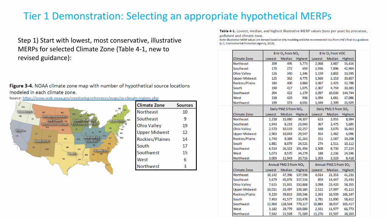
Step 1) Start with lowest, most conservative, illustrative MERPs for selected Climate Zone (Table 4-1, new to revised guidance):
Tier 1 Demonstration: Selecting an appropriate hypothetical MERPs

Step 2) Screen the closest hypothetical sources to the project facility and select the lowest, most conservative, MERPs
Tier 1 Demonstration: Selecting an appropriate hypothetical MERPs

12WUS1 12EUS2 12EUS3
12US2

Step 3) If selecting a nearby hypothetical source that is not the most conservative, the applicant should describe how the existing modeling reflects the formation of O3 or PM2.5 in that geographic area and is therefore most appropriate.
Information that could be used to describe the comparability of two different geographic areas include:• nearby local and regional sources of pollutants and their emissions (e.g., other industry, mobile, biogenics) • rural or urban nature of the area • terrain • ambient concentrations of relevant pollutants where available• average and peak temperatures • humidity
Tier 1 Demonstration: Selecting an appropriate hypothetical MERPs
Table A-1. Complete list of EPA modeled hypothetical sources presented in this document. “Max Nearby Urban (%)” column provides the highest percentage urban landcover in any grid cell near (within 50 km) the source.

MERP (tpy) =𝑎𝑎𝑎𝑎𝑎𝑎𝑎𝑎𝑎𝑎𝑎𝑎𝑎𝑎𝑎𝑎𝑎𝑎𝑎𝑎 𝑆𝑆𝑆𝑆𝑆𝑆 𝑣𝑣𝑎𝑎𝑎𝑎𝑣𝑣𝑎𝑎 (𝑎𝑎𝑎𝑎𝑎𝑎 𝑜𝑜𝑜𝑜 𝑢𝑢𝑢𝑢𝑚𝑚𝑚
) ∗ 𝑀𝑀𝑀𝑀𝑀𝑀𝑀𝑀𝑀𝑀𝑀𝑀𝑀𝑀 𝑀𝑀𝑚𝑚𝑒𝑒𝑒𝑒𝑒𝑒𝑒𝑒𝑀𝑀𝑒𝑒 𝑟𝑟𝑟𝑟𝑟𝑟𝑀𝑀 𝑟𝑟𝑡𝑡𝑡𝑡 𝑓𝑓𝑟𝑟𝑀𝑀𝑚𝑚 ℎ𝑡𝑡𝑡𝑡𝑀𝑀𝑟𝑟ℎ𝑀𝑀𝑟𝑟𝑒𝑒𝑦𝑦𝑟𝑟𝑀𝑀 𝑒𝑒𝑀𝑀𝑢𝑢𝑟𝑟𝑦𝑦𝑀𝑀𝑀𝑀𝑀𝑀𝑀𝑀𝑀𝑀𝑀𝑀𝑀𝑀𝑀𝑀 𝑟𝑟𝑒𝑒𝑟𝑟 𝑞𝑞𝑢𝑢𝑟𝑟𝑀𝑀𝑒𝑒𝑟𝑟𝑡𝑡 𝑒𝑒𝑚𝑚𝑡𝑡𝑟𝑟𝑦𝑦𝑟𝑟 𝑡𝑡𝑡𝑡𝑝𝑝 𝑀𝑀𝑟𝑟 𝑢𝑢𝑢𝑢
𝑚𝑚𝑚 𝑓𝑓𝑟𝑟𝑀𝑀𝑚𝑚 ℎ𝑡𝑡𝑡𝑡𝑀𝑀𝑟𝑟ℎ𝑀𝑀𝑟𝑟𝑒𝑒𝑦𝑦𝑟𝑟𝑀𝑀 𝑒𝑒𝑀𝑀𝑢𝑢𝑟𝑟𝑦𝑦𝑀𝑀
MERP (tpy) = 1.2 𝑢𝑢𝑢𝑢𝑚𝑚𝑚
∗ 1000 𝑟𝑟𝑡𝑡𝑡𝑡𝑚.271 𝑢𝑢𝑢𝑢
𝑚𝑚𝑚= 367 tpy MERP (tpy) = 1.0 ppb ∗ 500 𝑟𝑟𝑡𝑡𝑡𝑡
1.1𝑚4 𝑡𝑡𝑡𝑡𝑝𝑝= 441 𝑡𝑡𝑎𝑎𝑡𝑡
Tier 1 Demonstration: Example MERPs Calculation
Class II Values
Metric Poll State County Emissions Stack Height Conc MERPDAILY SULFATE Florida Bay 1000 10 3.271 367
Metric Poll State County Emissions Stack Height Conc MERPO3 MDA8 NOX Florida Bay 500 10 1.134 441

FL Project Source
Tier 1 Demonstration: PM2.5 24-hr SIL ExampleExample: A small, surface-level source in central Florida with 100 tpy of NOx and 100 tpy of SO2 with 1.0 𝒖𝒖𝒖𝒖
𝒎𝒎𝒎𝒎modeled
concentration of Primary PM2.5 for the 24-hr Class II SIL.

NOX and SO2 precursor contributions to secondary PM2.5 are considered together, in addition to modeled primary PM2.5, to determine if the source’s air quality impact would exceed the PM2.5 SIL.
Equations to assess Project emission secondary impacts:
Project Impact as % of SIL = 𝐸𝐸𝑚𝑚𝑒𝑒𝑒𝑒𝑒𝑒𝑒𝑒𝑀𝑀𝑒𝑒 𝑟𝑟𝑟𝑟𝑟𝑟𝑀𝑀 𝑟𝑟𝑡𝑡𝑡𝑡 𝑓𝑓𝑟𝑟𝑀𝑀𝑚𝑚 𝑃𝑃𝑟𝑟𝑀𝑀𝑃𝑃𝑀𝑀𝑦𝑦𝑟𝑟𝑀𝑀𝐸𝐸𝑀𝑀𝑃𝑃 𝑟𝑟𝑡𝑡𝑡𝑡 𝑓𝑓𝑟𝑟𝑀𝑀𝑚𝑚 ℎ𝑡𝑡𝑡𝑡𝑀𝑀𝑟𝑟ℎ𝑀𝑀𝑟𝑟𝑒𝑒𝑦𝑦𝑟𝑟𝑀𝑀 𝑆𝑆𝑀𝑀𝑢𝑢𝑟𝑟𝑦𝑦𝑀𝑀
* 100
Project Impact in ppb or 𝑢𝑢𝑢𝑢𝑚𝑚𝑚
= 𝐸𝐸𝑚𝑚𝑒𝑒𝑒𝑒𝑒𝑒𝑒𝑒𝑀𝑀𝑒𝑒 𝑟𝑟𝑟𝑟𝑟𝑟𝑀𝑀 𝑟𝑟𝑡𝑡𝑡𝑡 𝑓𝑓𝑟𝑟𝑀𝑀𝑚𝑚 𝑃𝑃𝑟𝑟𝑀𝑀𝑃𝑃𝑀𝑀𝑦𝑦𝑟𝑟𝑀𝑀𝐸𝐸𝑀𝑀𝑃𝑃 𝑟𝑟𝑡𝑡𝑡𝑡 𝑓𝑓𝑟𝑟𝑀𝑀𝑚𝑚 ℎ𝑡𝑡𝑡𝑡𝑀𝑀𝑟𝑟ℎ𝑀𝑀𝑟𝑟𝑒𝑒𝑦𝑦𝑟𝑟𝑀𝑀 𝑒𝑒𝑀𝑀𝑢𝑢𝑟𝑟𝑦𝑦𝑀𝑀
∗ 𝑎𝑎𝑎𝑎𝑎𝑎𝑎𝑎𝑎𝑎𝑎𝑎𝑎𝑎𝑎𝑎𝑎𝑎𝑎𝑎 𝑆𝑆𝑆𝑆𝑆𝑆 𝑣𝑣𝑎𝑎𝑎𝑎𝑣𝑣𝑎𝑎 (𝑎𝑎𝑎𝑎𝑎𝑎 𝑜𝑜𝑜𝑜 𝑢𝑢𝑢𝑢𝑚𝑚𝑚
)
Project Impact in ppb or 𝑢𝑢𝑢𝑢𝑚𝑚𝑚
= 𝐸𝐸𝐸𝐸𝑎𝑎𝐸𝐸𝐸𝐸𝑎𝑎𝑜𝑜𝐸𝐸 𝑜𝑜𝑎𝑎𝑡𝑡𝑎𝑎 𝑡𝑡𝑎𝑎𝑡𝑡 𝑓𝑓𝑜𝑜𝑜𝑜𝐸𝐸 𝑃𝑃𝑜𝑜𝑜𝑜𝑃𝑃𝑎𝑎𝑎𝑎𝑡𝑡 ∗ 𝑀𝑀𝑀𝑀𝑀𝑀𝑀𝑀𝑀𝑀𝑀𝑀𝑀𝑀 𝑟𝑟𝑒𝑒𝑟𝑟 𝑞𝑞𝑢𝑢𝑟𝑟𝑀𝑀𝑒𝑒𝑟𝑟𝑡𝑡 𝑒𝑒𝑚𝑚𝑡𝑡𝑟𝑟𝑦𝑦𝑟𝑟 𝑓𝑓𝑟𝑟𝑀𝑀𝑚𝑚 ℎ𝑡𝑡𝑡𝑡𝑀𝑀𝑟𝑟ℎ𝑀𝑀𝑟𝑟𝑒𝑒𝑦𝑦𝑟𝑟𝑀𝑀 𝑒𝑒𝑀𝑀𝑟𝑟𝑢𝑢𝑦𝑦𝑀𝑀𝑀𝑀𝑀𝑀𝑀𝑀𝑀𝑀𝑀𝑀𝑀𝑀𝑀𝑀 𝑀𝑀𝑚𝑚𝑒𝑒𝑒𝑒𝑒𝑒𝑒𝑒𝑀𝑀𝑒𝑒 𝑟𝑟𝑟𝑟𝑟𝑟𝑀𝑀 (𝑟𝑟𝑡𝑡𝑡𝑡) 𝑓𝑓𝑟𝑟𝑀𝑀𝑚𝑚 ℎ𝑡𝑡𝑡𝑡𝑀𝑀𝑟𝑟ℎ𝑀𝑀𝑟𝑟𝑒𝑒𝑦𝑦𝑟𝑟𝑀𝑀 𝑒𝑒𝑀𝑀𝑢𝑢𝑟𝑟𝑦𝑦𝑀𝑀
Tier 1 Demonstration: PM2.5 24-hr SIL Example

Is Primary + Secondary PM2.5 > SIL?
Step 1): Use lowest illustrative MERP from the Southeast Climate Zone:
Tier 1 Demonstration: PM2.5 24-hr SIL Example
PM2.5 24-hr SIL = 1.2 𝒖𝒖𝒖𝒖𝒎𝒎𝒎𝒎
Example: A small, surface-level source in central Florida with 100 tpy of NOx and 100 tpy of SO2 with 1.0 𝒖𝒖𝒖𝒖𝒎𝒎𝒎𝒎
modeled concentration of Primary PM2.5 for the 24-hr Class II SIL.

Tier 1 Demonstration: PM2.5 24-hr SIL ExampleExample: A small, surface-level source in central Florida with 100 tpy of NOx and 100 tpy of SO2 with 1.0 𝒖𝒖𝒖𝒖
𝒎𝒎𝒎𝒎modeled
concentration of Primary PM2.5 for the 24-hr Class II SIL.
Step 1): Use lowest illustrative MERP from the Southeast Climate Zone:
Project Impact as % of SIL =( 100 𝑟𝑟𝑡𝑡𝑡𝑡 𝑁𝑁𝑁𝑁𝑁𝑁 𝑓𝑓𝑟𝑟𝑀𝑀𝑚𝑚 𝑒𝑒𝑀𝑀𝑢𝑢𝑟𝑟𝑦𝑦𝑀𝑀1,94𝑚 𝑟𝑟𝑡𝑡𝑡𝑡 𝑁𝑁𝑁𝑁𝑁𝑁 𝑀𝑀𝑟𝑟𝑒𝑒𝑀𝑀𝑡𝑡 𝑃𝑃𝑀𝑀2.5𝑀𝑀𝐸𝐸𝑀𝑀𝑃𝑃
+ 100 𝑟𝑟𝑡𝑡𝑡𝑡 𝑆𝑆𝑁𝑁2 𝑓𝑓𝑟𝑟𝑀𝑀𝑚𝑚 𝑒𝑒𝑀𝑀𝑢𝑢𝑟𝑟𝑦𝑦𝑀𝑀𝑚67 𝑇𝑇𝑃𝑃𝑇𝑇 𝑆𝑆𝑁𝑁2 𝑀𝑀𝑟𝑟𝑒𝑒𝑀𝑀𝑡𝑡 𝑃𝑃𝑀𝑀2.5 𝑀𝑀𝐸𝐸𝑀𝑀𝑃𝑃
) * 100 = 32% of SIL
Project Impact in 𝑢𝑢𝑢𝑢𝑚𝑚𝑚
= ( 100 𝑟𝑟𝑡𝑡𝑡𝑡 𝑁𝑁𝑁𝑁𝑁𝑁 𝑓𝑓𝑟𝑟𝑀𝑀𝑚𝑚 𝑒𝑒𝑀𝑀𝑢𝑢𝑟𝑟𝑦𝑦𝑀𝑀1,94𝑚 𝑟𝑟𝑡𝑡𝑡𝑡 𝑁𝑁𝑁𝑁𝑁𝑁 𝑀𝑀𝑟𝑟𝑒𝑒𝑀𝑀𝑡𝑡 𝑃𝑃𝑀𝑀2.5 𝑀𝑀𝐸𝐸𝑀𝑀𝑃𝑃
+ 100 𝑟𝑟𝑡𝑡𝑡𝑡 𝑆𝑆𝑁𝑁2 𝑓𝑓𝑟𝑟𝑀𝑀𝑚𝑚 𝑒𝑒𝑀𝑀𝑢𝑢𝑟𝑟𝑦𝑦𝑀𝑀𝑚67 𝑇𝑇𝑃𝑃𝑇𝑇 𝑆𝑆𝑁𝑁2 𝑀𝑀𝑟𝑟𝑒𝑒𝑀𝑀𝑡𝑡 𝑃𝑃𝑀𝑀2.5𝑀𝑀𝐸𝐸𝑀𝑀𝑃𝑃
) * 1.2 𝑢𝑢𝑢𝑢𝑚𝑚𝑚
= 0.384 𝒖𝒖𝒖𝒖𝒎𝒎𝒎𝒎
Primary + Secondary PM2.5 as % of SIL:1.0𝑢𝑢𝑢𝑢𝑚𝑚𝑚𝑚𝑚𝑀𝑀𝑀𝑀𝑀𝑀𝑀𝑀𝑀𝑀𝑀𝑀
1.2𝑢𝑢𝑢𝑢𝑚𝑚𝑚 𝑆𝑆𝑆𝑆𝑆𝑆+ 0.32 = 115% of SIL
Primary + Secondary PM2.5 in 𝑢𝑢𝑢𝑢𝑚𝑚𝑚
:
1.0 𝑢𝑢𝑢𝑢𝑚𝑚𝑚
+ 0.384 𝑢𝑢𝑢𝑢𝑚𝑚𝑚
= 1.384 𝐮𝐮𝐮𝐮𝐦𝐦𝒎𝒎

Is Primary + Secondary PM2.5 > SIL?1.0 + 0.38 = 1.38 𝐮𝐮𝐮𝐮
𝐦𝐦𝒎𝒎
If no, then total PM2.5daily is below the SIL and no Class II Increment or NAAQS analysis is necessary
Step 2: Select lowest MERP from nearby sources with similar stack height:
Step 1): Use lowest, illustrative MERP from the Southeast Climate Zone:
100 tpy NOx from source/1,943 tpy NOx daily PM2.5 MERP = 0.05100 tpy SO2 from source/367 tpy SO2 daily PM2.5 MERP = 0.27 Total Secondary PM2.5 = .05 + .27 = .32 * 100 = 32% or 0.32 * 1.2 ug
m𝑚= 0.384 𝐮𝐮𝐮𝐮
𝐦𝐦𝒎𝒎
Tier 1 Demonstration: PM2.5 24-hr SIL ExampleExample: A small, surface-level source in central Florida with 100 tpy of NOx and 100 tpy of SO2 with 1.0 𝒖𝒖𝒖𝒖
𝒎𝒎𝒎𝒎modeled
concentration of Primary PM2.5 for the 24-hr Class II SIL.
PM2.5 24-hr SIL = 1.2 𝒖𝒖𝒖𝒖𝒎𝒎𝒎𝒎

Tier 1 Demonstration: PM2.5 24-hr SIL Example
Step 2): Select lowest MERP from nearby sources with similar stack height:
-Florida, Bay (12EUS2):-Alabama, Tallapoosa (12EUS3):-Alabama, Autauga (12EU2):
Metric Poll State County Emissions Stack Height Conc MERPDAILY NITRATE Florida Bay 1000 10 0.618 1943DAILY NITRATE Florida Bay 500 10 0.283 2122DAILY NITRATE Alabama Autauga 500 10 0.178 3370DAILY NITRATE Alabama Autauga 1000 10 0.341 3514DAILY NITRATE Alabama Tallapoosa 500 10 0.092 6555
Metric Poll State County Emissions Stack Height Conc MERPDAILY SULFATE Florida Bay 1000 10 3.271 367DAILY SULFATE Alabama Autauga 1000 10 3.097 387DAILY SULFATE Florida Bay 500 10 1.366 439DAILY SULFATE Alabama Autauga 500 10 1.231 487DAILY SULFATE Alabama Tallapoosa 500 10 0.325 1844
Same MERPs from Step 1; therefore:
Total Secondary PM2.5 = 0.384 ugm𝑚
or 32% of SIL
Total PM2.5 = 1.0 + 0.38 = 1.38 𝐮𝐮𝐮𝐮𝐦𝐦𝒎𝒎
Example: A small, surface-level source in central Florida with 100 tpy of NOx and 100 tpy of SO2 with 1.0 𝒖𝒖𝒖𝒖𝒎𝒎𝒎𝒎
modeled concentration of Primary PM2.5 for the 24-hr Class II SIL.

Is Primary + Secondary PM2.5 > SIL?1.0 + 0.38 = 1.38 𝒖𝒖𝒖𝒖
𝒎𝒎𝒎𝒎
Then Total PM2.5 Daily is below the SIL and no Class II Increment or NAAQS analysis is necessary
Step 2: Select lowest MERP from nearby sources with similar stack height:-Florida, Bay (12EUS2):-Alabama, Tallapoosa (12EUS3):-Alabama, Autauga (12EU2):
Same as Step 1:
Total Secondary PM2.5 = 0.384 ug/m3 or 32% of SILTotal PM2.5 = 1.0 + 0.38 = 1.38 𝒖𝒖𝒖𝒖
𝒎𝒎𝒎𝒎
Step 3): Select most representative nearby source for similar scenario (500 tpy and L stack):
Step 1): Use lowest illustrative MERP from the Southeast Climate Zone:
100 tpy NOx from source/1,943 tpy NOx daily PM2.5 MERP = 0.05100 tpy SO2 from source/367 TPY SO2 daily PM2.5 MERP = 0.27 Total Secondary PM2.5 = .05 + .27 = .32 * 100 = 32% or 0.32 * 1.2 ug
m𝑚= 0.384 𝒖𝒖𝒖𝒖
𝒎𝒎𝒎𝒎
Tier 1 Demonstration: PM2.5 24-hr SIL ExampleExample: A small, surface-level source in central Florida with 100 tpy of NOx and 100 tpy of SO2 with 1.0 𝒖𝒖𝒖𝒖
𝒎𝒎𝒎𝒎modeled
concentration of Primary PM2.5 for the 24-hr Class II SIL.
PM2.5 24-hr SIL = 1.2 𝒖𝒖𝒖𝒖𝒎𝒎𝒎𝒎

Tier 1 Demonstration: PM2.5 24-hr SIL Example
Step 3): Select most representative nearby source for similar scenario (500 tpy and L stack):
-Florida, Bay (12EUS2):-Alabama, Tallapoosa (12EUS3):-Alabama, Autauga (12EU2):
Information that could be used to assess the comparability of two different geographic areas include:• nearby local and regional sources of pollutants and
their emissions (e.g., other industry, mobile, biogenics)
• rural or urban nature of the area • terrain features• ambient concentrations of relevant pollutants
where available• average and peak temperatures • humidity
Metric Poll State County Emissions Stack Height Conc MERPDAILY NITRATE Florida Bay 500 10 0.283 2122DAILY NITRATE Alabama Autauga 500 10 0.178 3370DAILY NITRATE Alabama Tallapoosa 500 10 0.092 6555
Metric Poll State County Emissions Stack Height Conc MERPDAILY SULFATE Florida Bay 500 10 1.366 439DAILY SULFATE Alabama Autauga 500 10 1.231 487DAILY SULFATE Alabama Tallapoosa 500 10 0.325 1844
100 𝑟𝑟𝑡𝑡𝑡𝑡 𝑁𝑁𝑁𝑁𝑁𝑁 𝑓𝑓𝑟𝑟𝑀𝑀𝑚𝑚 𝑒𝑒𝑀𝑀𝑢𝑢𝑟𝑟𝑦𝑦𝑀𝑀6,555 𝑟𝑟𝑡𝑡𝑡𝑡 𝑁𝑁𝑁𝑁𝑁𝑁 𝑀𝑀𝑟𝑟𝑒𝑒𝑀𝑀𝑡𝑡 𝑃𝑃𝑀𝑀2.5 𝑀𝑀𝐸𝐸𝑀𝑀𝑃𝑃
= 0.015
100 𝑟𝑟𝑡𝑡𝑡𝑡 𝑆𝑆𝑁𝑁2 𝑓𝑓𝑟𝑟𝑀𝑀𝑚𝑚 𝑒𝑒𝑀𝑀𝑢𝑢𝑟𝑟𝑦𝑦𝑀𝑀1,844 𝑇𝑇𝑃𝑃𝑇𝑇 𝑆𝑆𝑁𝑁2 𝑀𝑀𝑟𝑟𝑒𝑒𝑀𝑀𝑡𝑡 𝑃𝑃𝑀𝑀2.5𝑀𝑀𝐸𝐸𝑀𝑀𝑃𝑃
= 0.05
Total Secondary PM2.5 = .015 + .05 = .065 * 100 = 7% of SILor 0.065 * 1.2 𝑢𝑢𝑢𝑢
𝑚𝑚𝑚= 0.078 𝒖𝒖𝒖𝒖
𝒎𝒎𝒎𝒎
Total PM2.5 = 1.0 + 0.078 = 1.078 𝒖𝒖𝒖𝒖𝒎𝒎𝒎𝒎 √
Example: A small, surface-level source in central Florida with 100 tpy of NOx and 100 tpy of SO2 with 1.0 𝒖𝒖𝒖𝒖𝒎𝒎𝒎𝒎
modeled concentration of Primary PM2.5 for the 24-hr Class II SIL.

Is Primary + Secondary PM2.5 > SIL?1.0 + 0.38 = 1.38 𝒖𝒖𝒖𝒖
𝒎𝒎𝒎𝒎
Then Total PM2.5 Daily is below the SIL and no Class II Increment or NAAQS analysis is necessary
Step 2: Select lowest MERP from nearby sources with similar stack height:-Florida, Bay (12EUS2):-Alabama, Tallapoosa (12EUS3):-Alabama, Autauga (12EUS2):
Same as Step 1:Total Secondary PM2.5 = 32% of SIL or 0.384 𝒖𝒖𝒖𝒖
𝒎𝒎𝒎𝒎Total PM2.5 = 1.0 + 0.38 = 1.38 𝒖𝒖𝒖𝒖
𝒎𝒎𝒎𝒎
Step 3): Select representative nearby source for similar scenario (500 tpy and L stack)-Florida, Bay (12EUS2):-Alabama, Tallapoosa (12EUS3):-Alabama, Autauga (12EU2):
NOx: 100 tpy/6555 MERP = 0.015SO2: 100 tpy/1844 MERP = 0.05Total Secondary PM2.5 = 7% of SIL or 0.078𝒖𝒖𝒖𝒖
𝒎𝒎𝒎𝒎Total PM2.5 = 1.0 + 0.078 = 1.078 𝒖𝒖𝒖𝒖
𝒎𝒎𝒎𝒎
Step 1): Use lowest illustrative MERP from the Southeast Climate Zone:
100 tpy NOx from source/1,943 tpy NOx daily PM2.5 MERP = 0.05100 tpy SO2 from source/367 TPY SO2 daily PM2.5 MERP = 0.27 Total Secondary PM2.5 = .05 + .27 = .32 * 100 = 32% or 0.32 * 1.2 ug/m3 = 0.384 𝒖𝒖𝒖𝒖
𝒎𝒎𝒎𝒎
Tier 1 Demonstration: PM2.5 24-hr SIL Example
√
Example: A small, surface-level source in central Florida with 100 tpy of NOx and 100 tpy of SO2 with 1.0 𝒖𝒖𝒖𝒖𝒎𝒎𝒎𝒎
modeled concentration of Primary PM2.5 for the 24-hr Class II SIL.
PM2.5 24-hr SIL = 1.2 𝒖𝒖𝒖𝒖𝒎𝒎𝒎𝒎

Tier 1 Demonstration: PM2.5 24-hr SIL Example
Is Primary + Secondary PM2.5 > 100% or 1.2 𝑢𝑢𝑢𝑢
𝑚𝑚𝑚?
Perform Cumulative Analysis
NAAQS Modeling:Modeled Primary PM2.5 + MERPs Secondary
PM2.5 + Background Monitor < NAAQS?
PSD Increment:Modeled Primary PM2.5 + MERPs Secondary
PM2.5 < Increment?
YES
PM2.5 24hr Analysis Complete
NO

Tier 1 Demonstration: Class I Analysis Example (Daily PM2.5) PM2.5 24-hr Class I SIL = 0.27 𝒖𝒖𝒖𝒖
𝒎𝒎𝒎𝒎
Example: A small, surface-level source in central Florida with 100 tpy of NOx and 100 tpy of SO2 with 𝟎𝟎.𝟏𝟏𝟖𝟖 𝒖𝒖𝒖𝒖𝒎𝒎𝒎𝒎
concentration of Primary PM2.5 at 50 km and the nearest Class I area is 150 km away
FL Source
Class I Area -Chassahowitzka
Use AERMOD to model primary PM2.5 at 50km in the direction of the nearest Class I area –Chassahowitzka, 150km away
Primary PM2.5 at 50 km = 𝟎𝟎.𝟏𝟏𝟖𝟖 𝒖𝒖𝒖𝒖
𝒎𝒎𝒎𝒎
Include Secondary PM2.5for Class I PM2.5assessments

Example: A small, surface-level source in central Florida with 100 tpy of NOx and 100 tpy of SO2 with 0.18 𝒖𝒖𝒖𝒖𝒎𝒎𝒎𝒎
concentration of Primary PM2.5 at 50 km and the nearest Class I area is 150 km away
Step 2) Select lowest MERP from nearby sources (Florida, Bay) with similar stack height:
Same as Step 1Total Secondary PM2.5 = .05 + .27 = 0.32 * 1.2 𝑢𝑢𝑢𝑢
𝑚𝑚𝑚= 0.384 𝒖𝒖𝒖𝒖
𝒎𝒎𝒎𝒎
Step 3): Select representative nearby source (Alabama, Tallapoosa) for similar scenario (500 tpy and L stack)
NOx: 100 tpy/6555 MERP = 0.015SO2: 100 tpy/1844 MERP = 0.05Total Secondary PM2.5 = 0.065 * 1.2 𝑢𝑢𝑢𝑢
𝑚𝑚𝑚= 0.078 𝒖𝒖𝒖𝒖
𝒎𝒎𝒎𝒎
Step 1) Use lowest illustrative MERP from the Southeast Climate Zone:
100 tpy NOx from source/1,943 tpy NOx daily PM2.5 MERP = 0.05100 tpy SO2 from source/367 TPY SO2 daily PM2.5 MERP = 0.27 Total Secondary PM2.5 = .05 + .27 = 0.32 * 1.2 𝑢𝑢𝑢𝑢
𝑚𝑚𝑚= 0.384 𝒖𝒖𝒖𝒖
𝒎𝒎𝒎𝒎
Tier 1 Demonstration: Class I Analysis Example (Daily PM2.5)
Primary PM2.5 at 50km + Secondary PM2.5 = 0.18 + 0.384 = 0.564 𝒖𝒖𝒖𝒖
𝒎𝒎𝒎𝒎
Primary PM2.5 at 50km + Secondary PM2.5 = 0.18 + 0.384 = 0.564 𝒖𝒖𝒖𝒖
𝒎𝒎𝒎𝒎
Primary PM2.5 at 50km + Secondary PM2.5 = 0.18 + 0.078 = 0.258 𝒖𝒖𝒖𝒖
𝒎𝒎𝒎𝒎
PM2.5 24-hr Class I SIL = 0.27 𝒖𝒖𝒖𝒖
𝒎𝒎𝒎𝒎
√

Tier 1 Demonstration: Class I Analysis Example (Daily PM2.5)Example: A small, surface-level source in central Florida with 100 tpy of NOx and 100 tpy of SO2 with 0.2 𝒖𝒖𝒖𝒖
𝒎𝒎𝒎𝒎concentration of Primary PM2.5 at 50 km and the nearest Class I area is 150 km away.
Step 3): Select representative nearby source (Alabama, Tallapoosa) for similar scenario (500 tpy and L stack)
NOx: 100 tpy/6555 MERP = 0.015SO2: 100 tpy/1844 MERP = 0.05Total Secondary PM2.5 = 0.065 * 1.2 𝑢𝑢𝑢𝑢
𝑚𝑚𝑚= 0.078 𝒖𝒖𝒖𝒖
𝒎𝒎𝒎𝒎
Primary PM2.5 at 50km + Secondary PM2.5 = 0.2 + 0.078 = 0.278 𝒖𝒖𝒖𝒖
𝒎𝒎𝒎𝒎
PM2.5 24-hr Class I SIL = 0.27 𝒖𝒖𝒖𝒖
𝒎𝒎𝒎𝒎
What to do when neither Step 1 – 3 will work and the nearest Class I area is significantly further than 50km?

The maximum predicted secondary concentrations are within 10 – 50 km of the source and decrease substantially with distance. Taking the conservative, maximum values from the MERPs may not work for all projects, requiring a more refined approach.

https://www.epa.gov/visibility/regional-haze-program

Alabama, Tallapoosa: 500 tpy, L Height (From MERPs Guidance Modeling)
Conc
entr
atio
n (u
g/m
3)
Distance from Source (Km)

Source 19: Alabama, TallapoosaEmissions: 500 TPY
Stack Height: L
Maximum Impact ≥ 50 km from source (ug/m3)
24-hr AnnualSulfate 0.2031 0.0041Nitrate 0.0626 0.0012
Tier 1 Demonstration: Class I Analysis Example (Daily PM2.5)Example: A small, surface-level source in central Florida with 100 tpy of NOx and 100 tpy of SO2 with 0.2 𝐮𝐮𝐮𝐮
𝐦𝐦𝒎𝒎concentration of Primary PM2.5 at 50 km and the nearest Class I area is 150 km away.
Refined Approach Step 1: Take the maximum impact ≥ 50 km from the hypothetical source and add to the primary PM2.5
Project Impact (𝑢𝑢𝑢𝑢𝑚𝑚𝑚
) = 𝐸𝐸𝐸𝐸𝑎𝑎𝐸𝐸𝐸𝐸𝑎𝑎𝑜𝑜𝐸𝐸 𝑜𝑜𝑎𝑎𝑡𝑡𝑎𝑎 𝑡𝑡𝑎𝑎𝑡𝑡 𝑓𝑓𝑜𝑜𝑜𝑜𝐸𝐸 𝑃𝑃𝑜𝑜𝑜𝑜𝑃𝑃𝑎𝑎𝑎𝑎𝑡𝑡 ∗ 𝑀𝑀𝑀𝑀𝑀𝑀𝑀𝑀𝑀𝑀𝑀𝑀𝑀𝑀 𝑟𝑟𝑒𝑒𝑟𝑟 𝑞𝑞𝑢𝑢𝑟𝑟𝑀𝑀𝑒𝑒𝑟𝑟𝑡𝑡 𝑒𝑒𝑚𝑚𝑡𝑡𝑟𝑟𝑦𝑦𝑟𝑟 𝑓𝑓𝑟𝑟𝑀𝑀𝑚𝑚 ℎ𝑡𝑡𝑡𝑡𝑀𝑀𝑟𝑟ℎ𝑀𝑀𝑟𝑟𝑒𝑒𝑦𝑦𝑟𝑟𝑀𝑀 𝑒𝑒𝑀𝑀𝑟𝑟𝑢𝑢𝑦𝑦𝑀𝑀𝑀𝑀𝑀𝑀𝑀𝑀𝑀𝑀𝑀𝑀𝑀𝑀𝑀𝑀 𝑀𝑀𝑚𝑚𝑒𝑒𝑒𝑒𝑒𝑒𝑒𝑒𝑀𝑀𝑒𝑒 𝑟𝑟𝑟𝑟𝑟𝑟𝑀𝑀 (𝑟𝑟𝑡𝑡𝑡𝑡) 𝑓𝑓𝑟𝑟𝑀𝑀𝑚𝑚 ℎ𝑡𝑡𝑡𝑡𝑀𝑀𝑟𝑟ℎ𝑀𝑀𝑟𝑟𝑒𝑒𝑦𝑦𝑟𝑟𝑀𝑀 𝑒𝑒𝑀𝑀𝑢𝑢𝑟𝑟𝑦𝑦𝑀𝑀
PM2.5 Nitrate Daily: 100 𝑡𝑡𝑎𝑎𝑡𝑡 ∗0.0626𝒖𝒖𝒖𝒖𝒎𝒎𝒎𝒎500 𝑟𝑟𝑡𝑡𝑡𝑡
= .013 𝑢𝑢𝑢𝑢𝑚𝑚𝑚
PM2.5 Sulfate Daily: 100 𝑡𝑡𝑎𝑎𝑡𝑡 ∗0.20𝑚1𝑢𝑢𝑢𝑢𝑚𝑚𝑚500 𝑟𝑟𝑡𝑡𝑡𝑡
= .041 𝑢𝑢𝑢𝑢𝑚𝑚𝑚
Total Secondary PM2.5 = .013 + .041 = .054 𝑢𝑢𝑢𝑢𝑚𝑚𝑚
Primary PM2.5 + Secondary PM2.5 = .20 + .054 = 0.254 𝒖𝒖𝒖𝒖𝒎𝒎𝒎𝒎
PM2.5 24-hr Class I SIL = 0.27 𝒖𝒖𝒖𝒖
𝒎𝒎𝒎𝒎

Tier 1 Demonstration: Class I Analysis Example (Daily PM2.5)Example: A small, surface-level source in central Florida with 100 tpy of NOx and 100 tpy of SO2 with 0.23 𝒖𝒖𝒖𝒖
𝒎𝒎𝒎𝒎concentration of Primary PM2.5 at 50 km and the nearest Class I area is 150 km away.
What if Step 1 refined screening was not enough?
Step 2: Take the maximum impact ≥ the distance the project facility is from the nearest Class I area and add to the primary PM2.5
Distance (km)24-hr Impact (µg/m3)
Nitrate Sulfate10 0.0702 0.258420 0.0915 0.325330 0.0821 0.305240 0.0720 0.258450 0.0492 0.155360 0.0626 0.203170 0.0501 0.150080 0.0389 0.109490 0.0306 0.0880
100 0.0287 0.0787110 0.0266 0.0590120 0.0256 0.0667130 0.0206 0.0577140 0.0235 0.0572150 0.0201 0.0571
Maximum Impact ≥ 150km:
PM2.5 Daily Nitrate: 100 tpy ∗ 0.0201 𝑢𝑢𝑢𝑢/𝑚𝑚𝑚500 𝑟𝑟𝑡𝑡𝑡𝑡
= .004 𝐮𝐮𝐮𝐮𝐦𝐦𝒎𝒎
PM2.5 Daily Sulfate: 100 tpy ∗ 0.0571 𝑢𝑢𝑢𝑢/𝑚𝑚𝑚500 𝑟𝑟𝑡𝑡𝑡𝑡
= .012 𝐮𝐮𝐮𝐮𝐦𝐦𝒎𝒎
Total Secondary PM2.5 = .004 + .012 = .016 𝐮𝐮𝐮𝐮𝐦𝐦𝒎𝒎
Primary PM2.5 + Secondary PM2.5 = .23 + .016 = .246 𝐮𝐮𝐮𝐮𝐦𝐦𝒎𝒎
PM2.5 24-hr Class I SIL = 0.27 𝒖𝒖𝒖𝒖
𝒎𝒎𝒎𝒎