Second Report by the United Kingdom under Article 17 - JNCCjncc.defra.gov.uk/pdf/FCS2007_techI_alphashapes.pdf · European Community Directive on the Conservation of Natural Habitats

European Community Directive

on the Conservation of Natural Habitats

and of Wild Fauna and Flora

(92/43/EEC)

Second Report by the United Kingdom under Article 17

on the implementation of the Directive from January 2001 to December 2006

Supporting documentation for making

Conservation status assessments: Technical Note I

AlphaShapes range calculation tool

Please note that this is a section of the report. For the complete report visit http://www.jncc.gov.uk/article17

Please cite as: Joint Nature Conservation Committee. 2007. Second Report by the UK under Article 17 on the implementation of the Habitats Directive from January 2001 to December 2006. Peterborough: JNCC. Available from: www.jncc.gov.uk/article17

http://www.jncc.gov.uk/article17

Technical Note I

AlphaShapes range calculation tool 1. Using Alpha Shapes for Conservation Status Reporting According to the guidance supplied by the EU the recommended method for estimating range for reporting on conservation status is to use a minimum convex polygon from a grid map. The UK is using the AlphaShapes range calculation tool (described in more detail below) to generate maps of range for the purposes of assessing conservation status. In calculating range the EU guidance states, “Small gaps in the distribution are considered as part of the range, but larger gaps in the distribution are considered as breaks in the range. There should be at least 4 or 5 non-occupied grids (about 40 – 50 km distance) to justify a break in the range.” The value of Alpha used to fit Alpha shapes to a particular feature is specified in the feature_range_parameters in the Access database. It is the radius of a circle (in km) which would just “slip through” a gap in the distribution (see Appendix 1 for explanation). So a value of 20 will cause gaps of more than 40km to appear as breaks in the range, a value of 25 will require gaps of over 50km for a break in the range. The value used for individual species and habitats range maps has been varied slightly to allow for knowledge about the ecology of habitats and the dispersal distances of species. The value of alpha ranges from 18 to 45 in the species conservation status assessments. This has been set to reflect the dispersal behaviour of individual species; to allow a buffer around incomplete records; and to provide the most realistic range estimate in the absence of complete census. For habitats, gaps in the distribution (normally comprising at least 4 or 5 non-occupied 10km squares; i.e. about 40 – 50 km distance) were treated as breaks in the range. The range envelope generated was clipped to exclude any areas that extended beyond the coastline over the sea. An additional clipping was applied to coastal habitats: this excluded any inland areas more than 10 km inland from the coastline. Details of the value of alpha used are given in the audit trails for individual assessments.

1 Second Report by the United Kingdom under Article 17 on the implementation of the Directive from

January 2001 to December 2006

Technical Note I

2. Introduction to the Range Map Tool The Range Map Tool takes the distribution of a habitat or species in the UK in the form of a simple list of grid squares at which it has been observed and fits one or more polygons representing the range of that feature. The area of the fitted range in km² is calculated. This is a measure of the “Extent of occurrence” in IUCN terms. The process has two parts:

• Fit an “alpha shape” around the distribution points. Alpha shapes are a family of polygons whose tightness of fit depends upon a parameter, α. The smaller the value of α, the tighter the fit until, at very small values, each distribution point becomes a separate polygon.

• Clip the alpha shape to exclude unsuitable areas – such as restricting the range of a terrestrial species to stop at the coast.

The tool is implemented as a program, which draws on data held in an access database to create the maps, while using separate files for clipping data, and generating maps as Gif files in a separate folder.



Technical Note I

3. Using AlphaShape When you open the program you should see a screen like this;

Controls: Database file: Path to the access database holding the 10km square

distribution data from which the tool draws the maps and calculates range. Values for range, in km2, are stored into this database each time the tool calculates them.

Path to clipping polygon: Path to the various clipping polygons. The following clipping options are available;

• 3km inside coastline • 3km outside coastline • 5km inside coastline • 5km outside coastline • 10km inside coastline • 10km outside coastline • 20km inside coastline • Clip to coastline

These options are activated by changing the column clipping_polygon_file_name in the table



Technical Note I

feature_range_parameters in the access database where the map data is stored.

Directory for map output: Path to the folder where the tool will store the maps generated as Gif files.

Map outline file: This is the file containing the coastal outline which will be drawn on the GIF images. For convenience, it uses the clip_coast.txt clipping polygon – so this field needs to specify the location of this file.

Features to recalculate List of features you can map. The tool draws on the data held in the access database in the form of 10km square distributions of Annex 1 features. This data can be modified or replaced (see adding data below). Select a feature or features from this list, and click on the “do it and close” button. This will cause the tool to create a map or maps and fit polygons to the points supplied. It will then save these maps as Gif files in the designated sub folder, calculate the range of the features selected, and save the newly calculated range figure to the access database in the table; feature_range_results. You are limited to choosing 20 features at once due to technical limitations in the program.

Outline: The colour of the line showing the outline of the coast of Great Britain and the Republic of Ireland. Click on the coloured rectangle to choose the colour for this line.

Show observations? Turns the display of the distribution points (the yellow squares) on and off. Click on the coloured rectangle to choose the colour for the distribution points.

Show clipped polygons? Turns the display of the clipped polygons on and off. Click on the coloured rectangle to choose the colour of the line used to draw the polygons.

Filled? Determines whether the clipped polygons are filled with colour or left as an outline. Click on the coloured rectangle to choose the colour to fill the polygons.



Technical Note I

4. Grid references The distribution of a feature is given in terms of presence in a square of the National Grid. The data collated for Report 312 was in the form of presence in 10km squares. This has consequences when trying to fit a range polygon. Consider some cases where small groups of 10km squares occur in isolation:

In the case of an isolated 10km square, if we fit to its centre, then the polygon will be a point and will have no area. It will “disappear” and not contribute any area to the extent of occurrence figure. If we consider its corners, then the fitted polygon will be the whole grid square and its contribution to the area will be the area of the grid square – 100km² if we are dealing with 10km square distribution points. In the case of a column or row of grid squares, if we fit to their centres, then we will see a fitted polygon which will appear as a straight line. So, again it won’t contribute any area. If we fit to the corners it will appear as a rectangular corridor and will contribute the number of grid squares in the row or column. In this case, a column of three 10km squares would contribute 300 km². In the case of the block of three grid squares arranged in a triangle, if we fit to centres we get a triangle of area 50 km². If we fit to corners, we get a much bigger shape whose area will contribute 350 km². The guidance from Europe suggests that the range should encompass the distribution points – i.e. fit the range to the corners of the grid squares. For this reason the range map tool automatically has the “Include grid square corners” option switched permanently on, which has the effect of fitting polygons to the corners of the distribution grid squares, meaning that isolated single grid squares and isolated rows and columns of grid squares, show up as polygons and contribute to the overall extent of



Technical Note I

occurrence area. However, the total extent of occurrence is considerably larger and may over-estimate the range area. The increase in total area caused by fitting to the corners of grid squares is greater if the grid squares are larger, so this effect will be greater for 10km square distribution data than when better resolution data is available.



Technical Note I

5. Adding your own data

5.1 Data format The distribution points to plot are stored in the database “habitats range maps data structure.mdb”, in the table “feature_distribution_data”. A separate database is used for species data. The format of the table is very simple:

• each row contains one distribution point, • the first cell in the row (headed featurecode) contains the name of the feature, i.e. a

habitat or species name, • the second cell in the row (headed gridtype) contains either GB or NI, depending on

whether the grid reference refers to a location in Great Britain or Northern Ireland, and tells the tool where the grid reference should be plotted,

• the third cell (headed gridref) contains a valid British or Irish grid reference of any precision (e.g. TL92, NT1735, H209883, etc.),

• the fourth cell (headed year) contains the year when the data was collected (this isn’t used by the range tool),

• the fifth cell (headed include) contains a tickbox, which is used to identify those rows to be included by the tool in calculating range for a particular feature,

• the sixth cell (headed source) identifies the source of the data in the table; a list of sources is held in a separate excel spreadsheet collected (this isn’t used by the range tool),

• the seventh cell (headed Date_collated) contains the year when the data was collated, • the eighth cell (headed Comment) is provided for supplementary information (e.g.

NVC type - this isn’t used by the range tool). The names in the first cell of every row for a given feature MUST be spelt and formatted in EXACTLY the same way (including spaces and any other punctuation). Otherwise each variation will be treated as a separate feature type! The following ways of writing grid references WILL NOT WORK!

• grids written so they contain spaces or other punctuation (e.g. TL 9823, TL 981 237), • BRC style numeric grid references (e.g. 52/9823), • x, y coordinates (e.g. 598,223), • tetrads (e.g. TL92B), • Channel Island grid refs (e.g. WA94).

5.2 Setting parameters for the analysis of a particular feature The table feature_range_parameters in the database controls the analysis of a feature. This table must contain an entry for each feature you want to analyse and map. If there is no entry in this table for a feature, it won’t appear in the output.



Technical Note I

featurecode This is the code by which a feature is identified, e.g. H1110 map_it Yes/no field. A map will be generated if this is ticked. alpha The value of α to use in fitting Alpha shapes to the distribution

points for this feature. This is the radius of the circles, described in Appendix 1, in km.

clipping_polygon_file_name The name of the clipping polygon to use for this feature. E.g. clip_coast.txt is used to clip the Alpha shapes to the coastal outline.

clipping_operation The operation to be used to combine the Alpha shape and the clipping polygon. 0 = Difference, 1 = Intersection, 2 = XOR, 3 = Union e.g. with clip_coast.txt specified as the clipping polygon and 1 as the operations, the resulting range will be the Intersection of the Alpha shapes and the coastal outline – i.e. only the parts of the Alpha shapes that fall within the coast. This restricts the range to terrestrial habitats. Using the same clipping polygon with an operation of 0 (difference), would restrict the range to those parts of the Alpha shapes that fall outside the coast – i.e. marine habitats.

date_parameters_set Set to today’s date if you change anything. Records when these parameters were last changed.

5.3 Results Apart from producing maps as GIF files in the designated directory (the one set in “Directory for map output:”), the results of area calculations are also written to the table feature_range_results in the Access database. featurecode This is the code by which a feature is identified, e.g. H1110 10km_square_count Number of different 10km squares found in the distribution

data for that feature (which had “include” flagged as True). alpha_shape_area Area of the fitted Alpha shapes in km2

clipped_shape_area Area of the clipped polygons in km2. This is the calculated range area.

last_calculated Date on which the calculations were last done DMapW_generated Date on which a 10km dot map was last generated for DMap

for Windows.



Technical Note I

Appendix 1: Understanding alpha shapes IUCN criteria for assessing threat to species make a distinction between two ways of measuring range: “Extent of occurrence is defined as the area contained within the shortest continuous imaginary boundary which can be drawn to encompass all the known, inferred or projected sites of present occurrence of a taxon, excluding cases of vagrancy. This measure may exclude discontinuities or disjunctions within the overall distribution of taxa (e.g. large areas of obviously unsuitable habitat).” “Area of occupancy is defined as the area within the ‘extent of occurrence’ which is occupied by a taxon, excluding cases of vagrancy. This measure reflects the fact that a taxon will not usually occur throughout the area of its extent of occurrence, which may contain unsuitable or unoccupied habitats.”

Extent of Occurrence The IUCN’s guidelines for using their Red List Categories and Criteria1 note that Extent of Occurrence can be measured by drawing a polygon around occupied sites and calculating its area. The simplest approach to this is to draw a figure known as a “convex hull” (the smallest polygon in which no internal angle exceeds 180o – conceptually, the shape you would get if you stuck a pin in each point and then stretched a rubber band around the outside of this group of pins). Here are examples applied to two species of Orthoptera from the BRC Grasshopper and Crickets recording scheme: the common field grasshopper (Chorthippus brunneus) and Roesel's bush cricket (Metrioptera roeselii):

1 http://intranet.iucn.org/webfiles/doc/SSC/RedList/RedListGuidelines.pdf



Technical Note I

Common field grasshopper (Chorthippus brunneus) Roesel's bush cricket (Metrioptera roeselii) It is immediately apparent that there are problems with using a convex hull to represent the Extent of Occurrences. In the first example of a common and widely distributed species, the convex hull includes huge areas of sea (an area of “obviously unsuitable habitat” for this terrestrial animal!) and will therefore greatly exaggerate the range. In the second example, the species has a much more restricted distribution, but the convex hull in this case is determined almost entirely by a few outlying colonies and again greatly exaggerates the area of the range. If we were using this measure of range to look at change over time, then there would potentially be a huge impact if, for example, one of the outlying colonies, like the one on the Welsh coast or the one in Morecambe Bay, was not included in one of the time periods. The IUCN’s guidelines, suggest that the way to resolve these issues is to use a more complex way of fitting a polygon known as an “alpha hull”. An alpha hull fits around the edges of the cloud of points more closely, the closeness of the fit being determined by a parameter, α.



Technical Note I

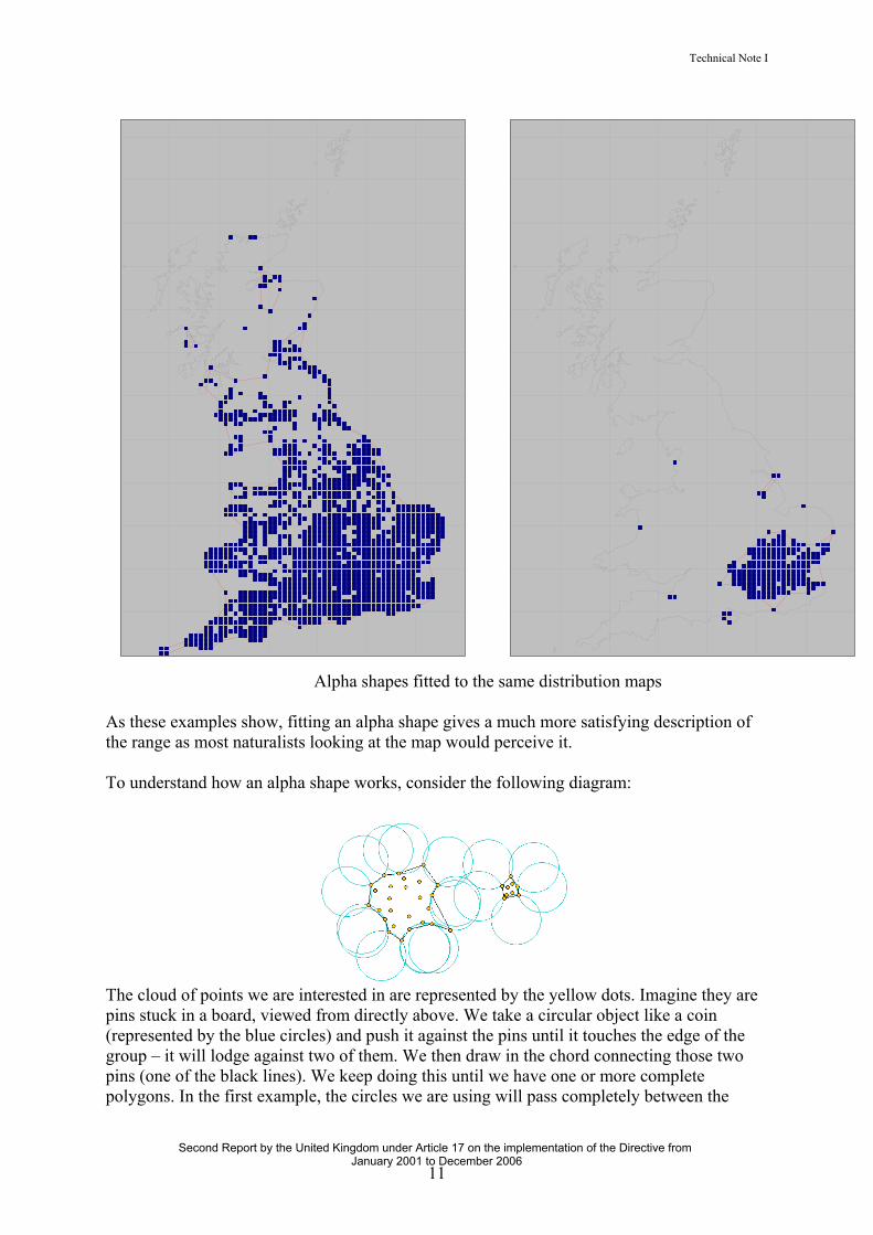
Alpha shapes fitted to the same distribution maps As these examples show, fitting an alpha shape gives a much more satisfying description of the range as most naturalists looking at the map would perceive it. To understand how an alpha shape works, consider the following diagram:

The cloud of points we are interested in are represented by the yellow dots. Imagine they are pins stuck in a board, viewed from directly above. We take a circular object like a coin (represented by the blue circles) and push it against the pins until it touches the edge of the group – it will lodge against two of them. We then draw in the chord connecting those two pins (one of the black lines). We keep doing this until we have one or more complete polygons. In the first example, the circles we are using will pass completely between the



Technical Note I

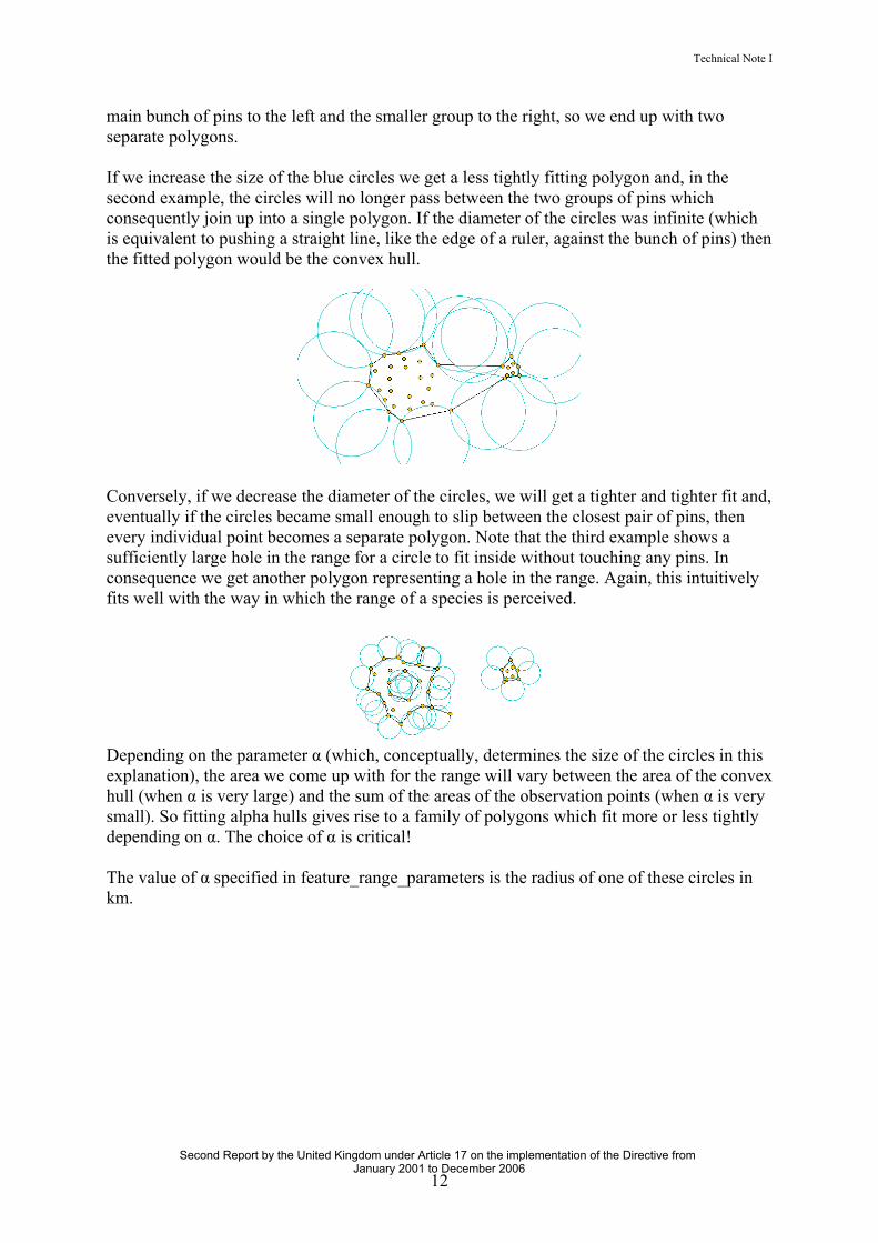
main bunch of pins to the left and the smaller group to the right, so we end up with two separate polygons. If we increase the size of the blue circles we get a less tightly fitting polygon and, in the second example, the circles will no longer pass between the two groups of pins which consequently join up into a single polygon. If the diameter of the circles was infinite (which is equivalent to pushing a straight line, like the edge of a ruler, against the bunch of pins) then the fitted polygon would be the convex hull.

Conversely, if we decrease the diameter of the circles, we will get a tighter and tighter fit and, eventually if the circles became small enough to slip between the closest pair of pins, then every individual point becomes a separate polygon. Note that the third example shows a sufficiently large hole in the range for a circle to fit inside without touching any pins. In consequence we get another polygon representing a hole in the range. Again, this intuitively fits well with the way in which the range of a species is perceived.

Depending on the parameter α (which, conceptually, determines the size of the circles in this explanation), the area we come up with for the range will vary between the area of the convex hull (when α is very large) and the sum of the areas of the observation points (when α is very small). So fitting alpha hulls gives rise to a family of polygons which fit more or less tightly depending on α. The choice of α is critical! The value of α specified in feature_range_parameters is the radius of one of these circles in km.



Documents

Second Report by the United Kingdom under Article 17 - JNCCjncc.defra.gov.uk/pdf/FCS2007_techI_alphashapes.pdf · European Community Directive on the Conservation of Natural Habitats