Embed Size (px)
Citation preview
Second-order Optimality Conditions for Mathematical Programs with
Equilibrium Constraints
Lei Guo, Gui-Hua Lin and Jane J. Ye
June 2012, Revised November 2012
Communicated by Michael Patriksson
Abstract. We study second-order optimality conditions for mathematical programs with equilibrium
constraints (MPEC). Firstly, we improve some second-order optimality conditions for standard nonlinear
programming problems using some newly discovered constraint qualifications in the literature, and apply
them to MPEC. Then, we introduce some MPEC variants of these new constraint qualifications, which
are all weaker than the MPEC linear independence constraint qualification, and derive several second-
order optimality conditions for MPEC under the new MPEC constraint qualifications. Finally, we discuss
the isolatedness of local minimizers for MPEC under very weak conditions.
Key Words. Mathematical program with equilibrium constraints, second-order optimality condition,
constraint qualification, isolatedness.
2010 Mathematics Subject Classification. 49K40, 90C26, 90C30, 90C33, 90C46.
1 Introduction
MPEC is a constrained optimization problem in which the essential constraints are defined by some
parametric variational inequalities or parametric complementarity systems. It plays a very important
role in many fields, such as engineering design, economic equilibria, transportation science, multilevel
game, and mathematical programming itself. However, this kind of problems is generally difficult to deal
with because its constraints fail to satisfy the standard Mangasarian-Fromovitz constraint qualification
(MFCQ) at any feasible point [1].
A lot of research has been done during the last two decades to study the first-order optimality
Lei Guo, School of Mathematical Sciences, Dalian University of Technology, Dalian 116024, China. E-mail:lei guo [email protected].
Gui-Hua Lin (corresponding author), School of Management, Shanghai University, Shanghai 200444, China. E-mail:[email protected].
Jane J. Ye, Department of Mathematics and Statistics, University of Victoria, Victoria, BC, V8W 3P4 Canada. E-mail:[email protected]
1

conditions for MPEC, such as Clarke (C-), Mordukhovich (M-), Strong (S-), Bouligrand (B-) stationarity
conditions; see, e.g., [1–8]. At the same time, algorithms for solving MPEC have been proposed by using
a number of approaches, such as sequential quadratic programming approach, penalty function approach,
relaxation approach, active set identification approach, etc.; see, e.g., [9–11] and the references therein
for more details.
In this paper, we focus on second-order optimality conditions for MPEC. First-order optimality
conditions tell us how the first derivatives of the functions involved are related to each other at locally
optimal solutions. However, for some feasible directions in the tangent cone such as the so-called critical
directions, we cannot determine from the first derivative information alone whether the objective
function increases or decreases in this direction. Second-order optimality conditions examine the second
derivative terms in the Taylor series expansions of the functions involved to see whether these extra
information resolves the issue of increase or decrease in the objective. Essentially, the second-order
optimality conditions are concerned with the curvature of the so-called MPEC Lagrangian function in
the critical directions. Moreover, second-order optimality conditions play important roles in
convergence analysis for numerical algorithms and the stability anslysis for MPEC; see, e.g., [12–18].
Compared with the first-order optimality conditions, there are very little research done with the
second-order optimality conditions for MPEC. Scheel and Scholtes [2] showed that S-stationary points
satisfying the refined second-order sufficient optimality conditions are strictly and locally optimal and
they derived a strong second-order necessary optimality condition under the MPEC strict MFCQ
(MPEC-SMFCQ). Izmailov [19] investigated second-order optimality conditions under the MPEC linear
independence constraint qualification (MPEC-LICQ). In this paper, we study second-order optimality
conditions for MPEC systematically. Note that, recently, several new constraint qualifications weaker
than the LICQ and MFCQ have been introduced for standard nonlinear programming problems. We
use these new constraint qualifications to derive some second-order optimality conditions for standard
nonlinear programming problems in Section 2 and apply the obtained results to MPEC. We further
introduce some MPEC variants of these new constraint qualifications, which are weaker than the
MPEC-LICQ, and derive some second-order optimality conditions for MPEC in terms of S- and
C-multipliers under these new MPEC constraint qualifications. Moreover, we establish some
relationships between various second-order optimality conditions for MPEC in terms of the classical
NLP multipliers and S-multipliers respectively. It is interesting to see that not all second-order
2

optimality conditions in terms of the classical NLP multipliers and S-multipliers are equivalent. In
addition, unlike the first-order conditions, the second-order conditions in terms of singular multipliers
provide some information for optimality. Finally, we discuss the isolatedness of local minimizers under
some weak conditions. Since MPEC includes standard nonlinear programming problems as special
cases, some of our results are new even for nonlinear programming problems.
2 Second-order Optimality Conditions for Standard Nonlinear
Programming Problems
In this section, we review and improve various second-order optimality conditions for the standard
nonlinear programming problem
min f(x) (1)
s.t. g(x) ≤ 0, h(x) = 0,
where f : IRn → IR, g : IRn → IRp, and h : IRn → IRq are all twice differentiable functions. Given r ≥ 0,
we let Lr be the generalized Lagrangian function for (1) defined by
Lr(x, y) := rf(x) + g(x)Tλ+ h(x)Tµ,
where y := (λ, µ). For a mapping ψ : IRn → IRl and a vector x ∈ IRn, we denote by ∇ψ(x) the transposed
Jacobian of ψ at x. According to the terminology used by Clarke [20], we call y an index r multiplier for
(1) at a feasible point x iff (r, y) 6= 0 and
∇xLr(x, y) = 0, λ ≥ 0, g(x)Tλ = 0.
An index 0 multiplier is usually referred to as a singular multiplier (see, e.g., [21]) or an abnormal
multiplier (see, e.g., [20]). Denote by F the feasible region of (1). For x∗ ∈ F , letMr(x∗) denote the set
of all index r multipliers for (1) at x∗ and I∗g := i | gi(x∗) = 0. Moreover, the linearized cone of F at
3

x∗ is defined by
L(x∗) := d ∈ IRn | ∇gi(x∗)T d ≤ 0 for i ∈ I∗g , ∇hj(x∗)T d = 0 for j = 1, . . . , q,
and the critical cone at x∗ is defined by
C(x∗) := d ∈ IRn | ∇f(x∗)T d ≤ 0 ∩ L(x∗),
respectively.
There are three types of second-order optimality conditions for (1). The definitions of strong second-
order optimality conditions are classical; see, e.g., [22,23]. The refined second-order optimality condition
was introduced in [24], and subsequently studied in [21]. The weak second-order optimality condition
was studied from theoretical and practical points of view in [25–27].
Definition 2.1 (Second-order optimality conditions for NLP) Let x∗ ∈ F .
(i) We say that the strong second-order necessary optimality condition (SSONC) holds at x∗ iff
M1(x∗) 6= ∅ and, for every y∗ ∈M1(x∗), there holds
dT∇2xL
1(x∗, y∗)d ≥ 0, ∀d ∈ C(x∗).
We say that the strong second-order sufficient optimality condition (SSOSC) holds at x∗ iff, for
every y∗ ∈M1(x∗), there holds
dT∇2xL
1(x∗, y∗)d > 0, ∀d ∈ C(x∗)\0.
(ii) We say that the refined second-order necessary optimality condition (RSONC) holds at x∗ iff, for
every d ∈ C(x∗), there exists y∗ ∈Mr(x∗) such that
dT∇2xL
r(x∗, y∗)d ≥ 0.
We say that the refined second-order sufficient optimality condition (RSOSC) holds at x∗ iff, for
4

every d ∈ C(x∗)\0, there exists y∗ ∈Mr(x∗) such that
dT∇2xL
r(x∗, y∗)d > 0.
(iii) We say that the weak second-order necessary optimality condition (WSONC) holds at x∗ iff there
exists y∗ ∈M1(x∗) such that
dT∇2xL
1(x∗, y∗)d ≥ 0, ∀d ∈ C(x∗),
where
C(x∗) := d | ∇gi(x∗)T d = 0 for i ∈ I∗g , ∇hj(x∗)T d = 0 for j = 1, . . . , q.
It is obvious that the following relationships hold:
SSOSC SSONC
⇓ ⇓ ⇓
RSOSC RSONC WSONC
Note that, for the sufficient optimality conditions to hold, no constraint qualification is required.
Proposition 2.1 (RSOSC for NLP) ( [21, Proposition 5.48]) Let x∗ ∈ F . If the RSOSC holds at x∗,
then x∗ is a locally optimal solution with quadratic growth, that is, there are constants c > 0 and δ > 0
such that
f(x) ≥ f(x∗) + c‖x− x∗‖2, ∀x ∈ F ∩ Bδ(x∗),
where Bδ(x∗) := x | ‖x− x∗‖ < δ with Euclidean vector norm ‖ · ‖.
However, for a necessary optimality condition to hold, a constraint qualification is required usually.
We next recall the definition of LICQ and its various relaxations. The CRCQ was introduced by Janin
in [28], and its relaxation RCRCQ was introduced by Minchenko and Stakhovski in [29]. The even
weaker WCR condition was introduced by Andreani et al in [30]. Note that the WCR condition is not a
constraint qualification [30].
Definition 2.2 (LICQ and its relaxations) Let x∗ ∈ F .
(i) We say that the linear independence constraint qualification (LICQ) holds at x∗ iff the family of
5
gradients ∇gi(x∗),∇hj(x∗) | i ∈ I∗g , j = 1, · · · , q is linearly independent.
(ii) We say that the constant rank constraint qualification (CRCQ) holds at x∗ iff there exists δ > 0 such
that, for each I ⊆ I∗g and J ⊆ 1, . . . , q, the family of gradients ∇gi(x),∇hj(x) | i ∈ I, j ∈ J
has the same rank for every x ∈ Bδ(x∗).
(iii) We say that the relaxed constant rank constraint qualification (RCRCQ) holds at x∗ iff there exists
δ > 0 such that, for each I ⊆ I∗g , the family of gradients ∇gi(x), ∇hj(x) | i ∈ I, j = 1, · · · , q has
the same rank for every x ∈ Bδ(x∗).
(iv) We say that the weak constant rank condition (WCR) holds at x∗ iff there exists δ > 0 such that the
family of gradients ∇gi(x),∇hj(x) | i ∈ I∗g , j = 1, · · · , q has the same rank for every x ∈ Bδ(x∗).
Recall that, for A := a1, · · · , al and B := b1, · · · , bs, (A,B) is said to be positively linearly
dependent iff there exist α and β such that α ≥ 0, (α, β) 6= 0, and
l∑i=1
αiai +
s∑j=1
βjbj = 0.
Otherwise, (A,B) is said to be positively linearly independent.
We now recall the positively linear independence constraint qualification (PLICQ) and its relaxations.
It is well-known that the MFCQ is equivalent to the PLICQ. The PLICQ is also called no nonzero
abnormal multiplier constraint qualification (NNAMCQ) or basic constraint qualification (Basic CQ).
The CPLD was introduced by Qi and Wei in [31] and was shown to be a constraint qualification by
Andreani et al. in [32]. The relaxed CPLD was introduced by Andreani et al. in [33]. The CRSC was
introduced by Andreani et al. in [34], and it is weaker than the RCPLD (see [34, Theorem 4.2]).
Definition 2.3 (MFCQ and its relaxations) Let x∗ ∈ F .
(i) We say that the positive linear independence constraint qualification (PLICQ) holds at x∗ iff the
family of gradients (∇gi(x∗) | i ∈ I∗g, ∇hj(x∗) | j = 1, · · · , q) is positively linearly independent.
(ii) We say that the constant positive linear dependence condition (CPLD) holds at x∗ iff, for each
I ⊆ I∗g and J ⊆ 1, . . . , q, whenever (∇gi(x∗) | i ∈ I, ∇hj(x∗) | j ∈ J ) is positively linearly
dependent, there exists δ > 0 such that, for every x ∈ Bδ(x∗), ∇gi(x),∇hj(x) | i ∈ I, j ∈ J is
linearly dependent.
6

(iii) Let J ⊆ 1, · · · , q be such that ∇hj(x∗)j∈J is a basis for span ∇hj(x∗)qj=1. We say that the
relaxed constant positive linear dependence condition (RCPLD) holds at x∗ iff there exists δ > 0
such that
– ∇hj(x)qj=1 has the same rank for each x ∈ Bδ(x∗);
– for each I ⊆ I∗g , if (∇gi(x∗) | i ∈ I, ∇hj(x∗) | j ∈ J ) is positively linearly dependent, then
∇gi(x),∇hj(x) | i ∈ I, j ∈ J is linearly dependent for each x ∈ Bδ(x∗).
(iv) Let J− := i ∈ I∗g | − ∇gi(x∗) ∈ L(x∗)o, where o stands for the polar operation. We say that the
constant rank of the subspace component condition (CRSC) holds at x∗ iff there exists δ > 0 such
that the family of gradients ∇gi(x),∇hj(x) | i ∈ J−, j ∈ 1, · · · , q has the same rank for every
x ∈ Bδ(x∗).
Note that the CPLD can be regarded as a complement for the PLICQ. In fact, it is easy to see
that the CPLD holds at x∗ if the PLICQ holds or, for each I ⊆ I∗g and J ⊆ 1, . . . , q, whenever
(∇gi(x∗) | i ∈ I, ∇hj(x∗) | j ∈ J ) is positively linearly dependent, there exists δ > 0 such that
∇gi(x),∇hj(x) | i ∈ I, j ∈ J is linearly dependent for every x ∈ Bδ(x∗). It is similar for the RCPLD
and CRSC. See [33,34] for the relations among the above constraint qualifications.
In the literature, the SSONC requires the LICQ. A counterexample due to Arutyunov [35] (see also
[36]) shows that one cannot relax LICQ to MFCQ. Recently, Minchenko and Stakhovski [29] showed that
the SSONC holds under the RCRCQ, which is weaker than the LICQ.
Proposition 2.2 (SSONC for NLP) [29, Theorem 6] Let x∗ be a locally optimal solution of (1). If
the RCRCQ holds at x∗, then x∗ satisfies the SSONC with r = 1.
In the following, we improve the standard results for the RSONC. We first give an equivalent form of
the Clarke calmness condition [20]. See [37] for the equivalence between the Clarke calmness and exact
penalization.
Definition 2.4 (Calmness) Let x∗ be a locally optimal solution of (1). We say that problem (1) is
(Clarke) calm at x∗ iff x∗ is also a locally optimal solution of the penalized problem
minx
f(x) + κ(maxg1(x), · · · , gp(x), 0+ ‖h(x)‖) (2)
7

for some positive constant κ.
Note that, since the concept involves the objective function, the calmness condition is not a constraint
qualification in the classical sense. It is just a sufficient condition under which the first-order conditions
and the RSONC with r = 1 hold at a local minimizer. The calmness condition may hold even when
Guignard constraint qualification [38], which is the weakest constraint qualification, does not hold. For
example, it is easy to verify that the optimization problem
min x1 + x2 s.t. (x1 − x2)2 = 0, x1 + 1 ≥ 0, x2 + 1 ≥ 0
is calm at the optimal solution (−1,−1), but the Guignard constraint qualification fails at the point.
The standard constraint qualification for the RSONC with r = 1 to hold at a local minimizer is the
MFCQ; see, e.g., [21]. The following theorem shows that the RSONC with r = 1 actually holds at a local
minimizer under the calmness condition.
Theorem 2.1 (RSONC for NLP) Let x∗ be a locally optimal solution of (1). Then the RSONC holds
at x∗. Moreover, if (1) is calm at x∗, then x∗ satisfies the RSONC with r = 1.
Proof. The fact that the RSONC holds at any local solution x∗ can be found in [21, Proposition 5.48].
We now suppose that (1) is calm at x∗. By the calmness condition, there exists κ > 0 such that x∗ is a
locally optimal solution of (2). It is easy to see that (x, t, s) = (x∗, 0, 0) is a locally optimal solution of
the problem
min f(x) + κ(t+
q∑j=1
sj)
s.t. t ≥ gi(x), i = 1, · · · , p,
t ≥ 0,
sj ≥ hj(x), sj ≥ −hj(x), j = 1, · · · , q.
It is straightforward to verify that the set of nonzero singular multipliers for the above problem at (x∗, 0, 0)
is empty, and hence the set of index 1 multipliers must be nonempty by virtue of the Fritz John necessary
optimality condition. It follows immediately that the MFCQ holds, and then the RSONC holds for the
above problem at (x∗, 0, 0) with r = 1. By direct calculation, the critical cone of the above problem at
8

(x∗, 0, 0) is
C(x∗, 0, 0) =
(d1, d2, d3)
∣∣∣∣∣∣∣∣∣∣∣∇f(x∗)T d1 + κd2 + κeT d3 ≤ 0, −d2 ≤ 0
∇gi(x∗)T d1 − d2 ≤ 0 i ∈ I∗g
∇hj(x∗)T d1 − d3j ≤ 0, −∇hj(x∗)T d1 − d3j ≤ 0 j = 1, · · · , q
.
For every d ∈ C(x∗), (d, 0, 0) ∈ C(x∗, 0, 0) holds clearly. On the other hand, the fact that (λg, µ, λh, λ−h) is
a multiplier for the above problem implies that (λg, λh−λ−h) is a multiplier for (1). It follows immediately
that the RSONC holds for (1) with r = 1.
Recently, Andreani et al. showed that the CRSC implies the existence of local error bound in [34,
Theorem 5.4]. It follows from the Clarke’s exact penalty principle [20, Proposition 2.4.3] that the existence
of local error bound implies the calmness condition; see, e.g., [3, Proposition 4.2]. Consequently, from
Theorem 2.1, we get the following result immediately. Note that, since the CRSC is much weaker than
the MFCQ, our result improves the classical result.
Corollary 2.1 (RSONC under CRSC) Let x∗ be a locally optimal solution of (1). If the CRSC
condition holds at x∗, then the RSONC holds at x∗ with r = 1.
Robinson [39] showed the isolatedness of KKT points under the condition that the MFCQ and SSOSC
hold. Qi and Wei [31] showed that a KKT point satisfying the CPLD and SSOSC in the sense of
Robinson [40], which is stronger than the one in this paper, is isolated. Since the RCPLD is weaker than
both CPLD and MFCQ, the following theorem improves the above results. Since the proof is a simplified
version of Theorem 4.1, we omit it here.
Theorem 2.2 (Isolatedness under RCPLD) Suppose that x∗ ∈ F is a KKT point, i.e.,M1(x∗) 6= ∅.
If the RCPLD and SSOSC hold at x∗, then x∗ is an isolated KKT point of (1).
Recall that the tangent cone of a set X at x∗ ∈ X is a closed cone defined by
TX(x∗) := d | ∃tk ≥ 0 and xk →X x∗ s.t. tk(xk − x∗)→ d,
where xk →X x∗ means that xk → x∗ with xk ∈ X for each k.
Lemma 2.1 [33, Theorem 3] If the RCPLD holds at x∗ ∈ F , then the Abadie CQ holds at x∗, i.e.,
9
TF (x∗) = LF (x∗).
The following result improves Theorem 3.1 of [30] in that the MFCQ assumption is replaced by the
weaker condition M1(x∗) 6= ∅.
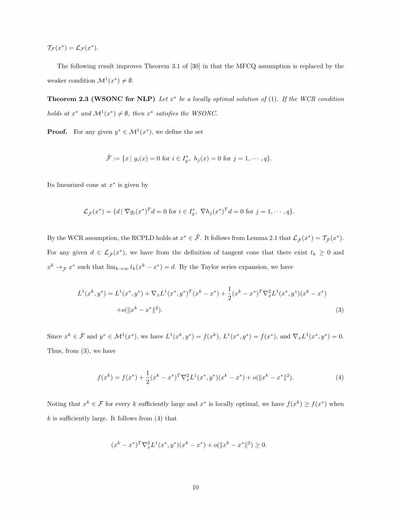
Theorem 2.3 (WSONC for NLP) Let x∗ be a locally optimal solution of (1). If the WCR condition
holds at x∗ and M1(x∗) 6= ∅, then x∗ satisfies the WSONC.
Proof. For any given y∗ ∈M1(x∗), we define the set
F := x | gi(x) = 0 for i ∈ I∗g , hj(x) = 0 for j = 1, · · · , q.
Its linearized cone at x∗ is given by
LF (x∗) = d | ∇gi(x∗)T d = 0 for i ∈ I∗g , ∇hj(x∗)T d = 0 for j = 1, · · · , q.
By the WCR assumption, the RCPLD holds at x∗ ∈ F . It follows from Lemma 2.1 that LF (x∗) = TF (x∗).
For any given d ∈ LF (x∗), we have from the definition of tangent cone that there exist tk ≥ 0 and
xk →F x∗ such that limk→∞ tk(xk − x∗) = d. By the Taylor series expansion, we have
L1(xk, y∗) = L1(x∗, y∗) +∇xL1(x∗, y∗)T (xk − x∗) +1
2(xk − x∗)T∇2
xL1(x∗, y∗)(xk − x∗)
+o(‖xk − x∗‖2). (3)
Since xk ∈ F and y∗ ∈ M1(x∗), we have L1(xk, y∗) = f(xk), L1(x∗, y∗) = f(x∗), and ∇xL1(x∗, y∗) = 0.
Thus, from (3), we have
f(xk) = f(x∗) +1
2(xk − x∗)T∇2
xL1(x∗, y∗)(xk − x∗) + o(‖xk − x∗‖2). (4)
Noting that xk ∈ F for every k sufficiently large and x∗ is locally optimal, we have f(xk) ≥ f(x∗) when
k is sufficiently large. It follows from (4) that
(xk − x∗)T∇2xL
1(x∗, y∗)(xk − x∗) + o(‖xk − x∗‖2) ≥ 0.
10

Multiplying it by t2k and taking a limit, we get the desired result.
Consider the mathematical program with equilibrium constraints (MPEC)
min f(x)
s.t. g(x) ≤ 0, h(x) = 0, (5)
0 ≤ G(x) ⊥ H(x) ≥ 0,
where f, g, h are assumed as above, G,H : IRn → IRm are all twice differentiable functions, and a ⊥ b
means that the vector a is perpendicular to the vector b. We can treat the MPEC (5) as the following
nonlinear programming problem with equality and inequality constraints:
min f(x)
s.t. g(x) ≤ 0, h(x) = 0, (6)
G(x) ≥ 0, H(x) ≥ 0, G(x)TH(x) ≤ 0.
In order to facilitate the notation, for a given feasible point x∗ of (6), we let I∗g be the same as above and
I∗ := i | Gi(x∗) = 0 < Hi(x
∗),
J ∗ := i | Gi(x∗) = 0 = Hi(x∗),
K∗ := i | Gi(x∗) > 0 = Hi(x∗).
Obviously, I∗,J ∗,K∗ is a partition of 1, 2, · · · ,m. For simplicity, we also denote by Lr, C, and Mr
the generalized Lagrangian, the critical cone, and the set of all r index multipliers of (6), respectively. It
is easy to distinguish them from the context. In particular, the generalized Lagrangian of (6) is
Lr(x, λ, µ, α, β, ξ) := rf(x) + g(x)Tλ+ h(x)Tµ−G(x)Tα−H(x)Tβ + ξG(x)TH(x),
11
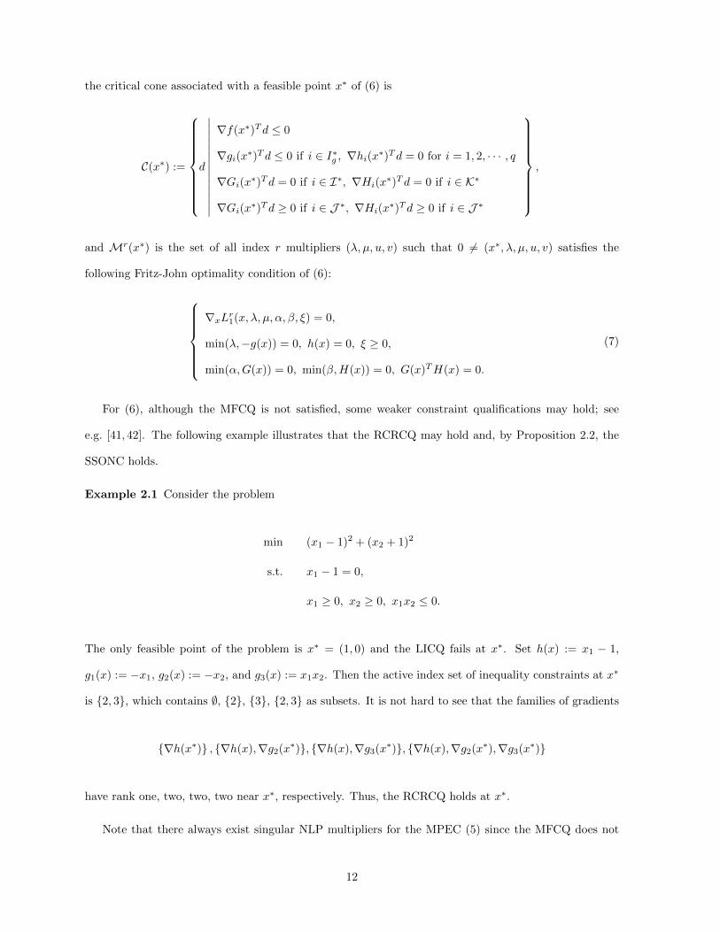
the critical cone associated with a feasible point x∗ of (6) is
C(x∗) :=
d
∣∣∣∣∣∣∣∣∣∣∣∣∣∣
∇f(x∗)T d ≤ 0
∇gi(x∗)T d ≤ 0 if i ∈ I∗g , ∇hi(x∗)T d = 0 for i = 1, 2, · · · , q
∇Gi(x∗)T d = 0 if i ∈ I∗, ∇Hi(x∗)T d = 0 if i ∈ K∗
∇Gi(x∗)T d ≥ 0 if i ∈ J ∗, ∇Hi(x∗)T d ≥ 0 if i ∈ J ∗
,
and Mr(x∗) is the set of all index r multipliers (λ, µ, u, v) such that 0 6= (x∗, λ, µ, u, v) satisfies the
following Fritz-John optimality condition of (6):
∇xLr1(x, λ, µ, α, β, ξ) = 0,
min(λ,−g(x)) = 0, h(x) = 0, ξ ≥ 0,
min(α,G(x)) = 0, min(β,H(x)) = 0, G(x)TH(x) = 0.
(7)
For (6), although the MFCQ is not satisfied, some weaker constraint qualifications may hold; see
e.g. [41, 42]. The following example illustrates that the RCRCQ may hold and, by Proposition 2.2, the
SSONC holds.
Example 2.1 Consider the problem
min (x1 − 1)2 + (x2 + 1)2
s.t. x1 − 1 = 0,
x1 ≥ 0, x2 ≥ 0, x1x2 ≤ 0.
The only feasible point of the problem is x∗ = (1, 0) and the LICQ fails at x∗. Set h(x) := x1 − 1,
g1(x) := −x1, g2(x) := −x2, and g3(x) := x1x2. Then the active index set of inequality constraints at x∗
is 2, 3, which contains ∅, 2, 3, 2, 3 as subsets. It is not hard to see that the families of gradients
∇h(x∗) , ∇h(x),∇g2(x∗), ∇h(x),∇g3(x∗), ∇h(x),∇g2(x∗),∇g3(x∗)
have rank one, two, two, two near x∗, respectively. Thus, the RCRCQ holds at x∗.
Note that there always exist singular NLP multipliers for the MPEC (5) since the MFCQ does not
12

hold at every feasible point. It is interesting that, although a singular NLP multiplier may not be useful
for first-order optimality, the second-order optimality conditions in terms of singular NLP multipliers
may provide useful information. We illustrate this point by using the following example.
Example 2.2 Consider the problem
min −x2
s.t. x1 − x2 = 0,
x1 ≥ 0, x2 ≥ 0, x1x2 ≤ 0.
The only feasible solution, which is certainly the only optimal solution, is x∗ = (0, 0). The critical cone
is
C(x∗) = d ∈ IR2 | − d2 ≤ 0, d1 − d2 = 0,−d1 ≤ 0,−d2 ≤ 0
= d ∈ IR2 | d1 = d2, d1 ≥ 0, d2 ≥ 0.
It is obvious that (µ, α, β, ξ) with µ = α = β = 0, ξ = 1 is a singular multiplier. For such a singular
multiplier, we have
∇2xL
0(x∗, µ, α, β, ξ) = ∇2ϕ(x1, x2) =
0 1
1 0
,
where ϕ(x1x2) := x1x2. Hence, for each d ∈ C(x∗) \ 0, we have d = (h, h) with h > 0. Therefore,
dT∇2xL
0(x∗, µ, α, β, ξ)d = 2h2 > 0
holds for each d ∈ C(x∗) \ 0. That is, the RSOSC with r = 0 is satisfied.
The above two examples illustrate that, in some cases, we can apply the standard results for NLP
to the MPEC (5) directly. However, since the Abadie CQ for (6) is only satisfied in fairly restrictive
circumstances (see, e.g., [42]) and the above constraint qualifications imply the Abadie CQ, it is more
reasonable to investigate the properties of (5) from the MPEC structure and specificity. In the next
13

section, we investigate the MPEC second-order optimality conditions.
3 MPEC Second-order Optimality Conditions
First, we review the first-order optimality conditions for MPEC. It is easy to see that the MPEC (5) can
be rewritten as the following optimization problem with a geometric constraint:
min f(x) (8)
s.t. F (x) ∈ Λ,
where
F (x) := (g(x), h(x),Ψ(x))T, Ψ(x) := (−G1(x),−H1(x), · · · ,−Gm(x),−Hm(x)),
and
Λ :=]−∞, 0]p × 0q × Cm, C := (a, b) ∈ IR2 | 0 ≤ −a ⊥ −b ≥ 0.
In the rest of the paper, we denote by X the feasible region of the MPEC (5) and define the generalized
MPEC-Lagrangian function of the MPEC (5) as
LrMPEC(x, λ, µ, u, v) := rf(x) + g(x)Tλ+ h(x)Tµ−G(x)Tu−H(x)T v
= rf(x) + F (x)T y, y := (λ, µ, u, v).
We need the following normal cones.
Definition 3.1 [43, 44] The regular normal cone of a set Ω ⊂ IRn at x∗ ∈ Ω is a closed convex cone
defined by
NΩ(x∗) := d | dT (x− x∗) ≤ o(‖x− x∗‖) for each x ∈ Ω,
14

and the limiting normal cone of Ω at x∗ ∈ Ω is a closed cone defined by
NΩ(x∗) := d | d = limk→∞
dk with dk ∈ NΩ(xk) and xk →Ω x∗.
Definition 3.2 [2, 4–6] Let x∗ ∈ X. We say that x∗ is Clarke stationary (C-stationary) to (5) iff there
exists (λ, µ, u, v) satisfying
∇xL1MPEC(x∗, λ, µ, u, v) = 0,
λ ≥ 0, g(x∗)Tλ = 0,
ui = 0, i ∈ K∗,
vi = 0, i ∈ I∗,
either uivi ≥ 0, i ∈ J ∗.
(9)
We say that x∗ is Mordukhovich stationary (M-stationary) to (5) iff there exists (λ, µ, u, v) satisfying
∇xL1MPEC(x∗, λ, µ, u, v) = 0,
λ ≥ 0, g(x∗)Tλ = 0,
ui = 0, i ∈ K∗,
vi = 0, i ∈ I∗,
either uivi = 0 or ui > 0, vi > 0, i ∈ J ∗.
(10)
We say that x∗ is strongly stationary (S-stationary) to (5) iff there exists (λ, µ, u, v) satisfying
∇xL1MPEC(x∗, λ, µ, u, v) = 0,
λ ≥ 0, g(x∗)Tλ = 0,
ui = 0, i ∈ K∗,
vi = 0, i ∈ I∗,
ui ≥ 0, vi ≥ 0, i ∈ J ∗.
(11)
By straightforward calculation, we can get the following result (see, e.g., [3, 8]).
15
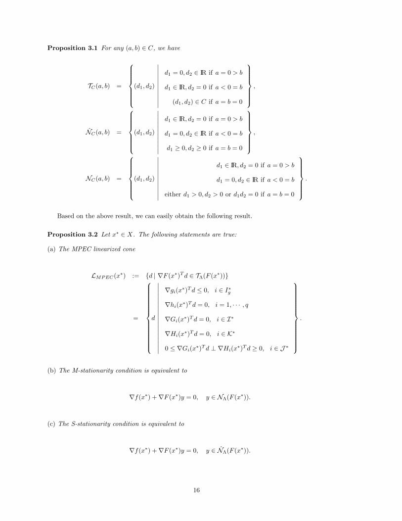
Proposition 3.1 For any (a, b) ∈ C, we have
TC(a, b) =
(d1, d2)
∣∣∣∣∣∣∣∣∣∣∣d1 = 0, d2 ∈ IR if a = 0 > b
d1 ∈ IR, d2 = 0 if a < 0 = b
(d1, d2) ∈ C if a = b = 0
,
NC(a, b) =
(d1, d2)
∣∣∣∣∣∣∣∣∣∣∣d1 ∈ IR, d2 = 0 if a = 0 > b
d1 = 0, d2 ∈ IR if a < 0 = b
d1 ≥ 0, d2 ≥ 0 if a = b = 0
,
NC(a, b) =
(d1, d2)
∣∣∣∣∣∣∣∣∣∣∣d1 ∈ IR, d2 = 0 if a = 0 > b
d1 = 0, d2 ∈ IR if a < 0 = b
either d1 > 0, d2 > 0 or d1d2 = 0 if a = b = 0
.
Based on the above result, we can easily obtain the following result.
Proposition 3.2 Let x∗ ∈ X. The following statements are true:
(a) The MPEC linearized cone
LMPEC(x∗) := d | ∇F (x∗)T d ∈ TΛ(F (x∗))
=
d
∣∣∣∣∣∣∣∣∣∣∣∣∣∣∣∣∣∣
∇gi(x∗)T d ≤ 0, i ∈ I∗g
∇hi(x∗)T d = 0, i = 1, · · · , q
∇Gi(x∗)T d = 0, i ∈ I∗
∇Hi(x∗)T d = 0, i ∈ K∗
0 ≤ ∇Gi(x∗)T d ⊥ ∇Hi(x∗)T d ≥ 0, i ∈ J ∗
.
(b) The M-stationarity condition is equivalent to
∇f(x∗) +∇F (x∗)y = 0, y ∈ NΛ(F (x∗)).
(c) The S-stationarity condition is equivalent to
∇f(x∗) +∇F (x∗)y = 0, y ∈ NΛ(F (x∗)).
16

We now study the second-order optimality conditions for the MPEC (5) by C-/M-/S-multipliers. To
this end, we define the MPEC critical cone at x∗ ∈ X as
CMPEC(x∗) := LMPEC(x∗) ∩ d | ∇f(x∗)T d ≤ 0. (12)
For a given x∗ ∈ X, we denote by MrS(x∗) the set of all index r S-multipliers (λ, µ, u, v) such that
(r, λ, µ, u, v) 6= 0 and (11) is satisfied with L1MPEC replaced by LrMPEC , denote byMr
M (x∗) the set of all
index r M-multipliers (λ, µ, u, v) such that (r, λ, µ, u, v) 6= 0 and (10) is satisfied with L1MPEC replaced by
LrMPEC , and denote byMrC(x∗) the set of all index r C-multipliers (λ, µ, u, v) such that (r, λ, µ, u, v) 6= 0
and (9) is satisfied with L1MPEC replaced by LrMPEC , respectively.
Definition 3.3 Let x∗ ∈ X.
(i) We say that the S-multiplier strong second-order necessary condition (S-SSONC) holds at x∗ iff
M1S(x∗) 6= ∅ and, for every y∗ ∈M1
S(x∗), there holds
dT∇2xL
1MPEC(x∗, y∗)d ≥ 0, ∀d ∈ CMPEC(x∗).
We say that the S-multiplier strong second-order sufficient condition (S-SSOSC) holds at x∗ iff, for
every y∗ ∈M1S(x∗), there holds
dT∇2xL
1MPEC(x∗, y∗)d > 0, ∀d ∈ CMPEC(x∗)\0.
(ii) We say that the S-multiplier refined second-order necessary condition (S-RSONC) holds at x∗ iff,
for every d ∈ CMPEC(x∗), there exists y∗ ∈MrS(x∗) such that
dT∇2xL
rMPEC(x∗, y∗)d ≥ 0.
We say that the S-multiplier refined second-order sufficient condition (S-RSOSC) holds at x∗ iff,
for every d ∈ CMPEC(x∗)\0, there exists y∗ ∈MrS(x∗) such that
dT∇2xL
rMPEC(x∗, y∗)d > 0.
17

(iii) We say that the S-multiplier weak second-order necessary condition (S-WSONC) holds at x∗ iff
there exists y∗ ∈M1S(x∗), there holds
dT∇2xL
1MPEC(x∗, y∗)d ≥ 0, ∀d ∈ CMPEC(x∗),
where
CMPEC(x∗) :=
d∣∣∣∣∣∣∣∇gi(x∗)T d = 0 if i ∈ I∗g , ∇hi(x∗)T d = 0 for i = 1, · · · , q
∇Gi(x∗)T d = 0 if i ∈ I∗ ∪ J ∗, ∇Hi(x∗)T d = 0 if i ∈ K∗ ∪ J ∗
.
It is well-known that there is a connection between the NLP multipliers and the S-multipliers; see,
e.g., [12,17]. We next investigate the connection between the classical second-order optimality condition
and the S-multiplier second-order optimality condition. Although the equation (13) in Theorem 3.1 is
given in [19, Proposition 1], we give a proof for completeness.
Theorem 3.1 (a) Let d ∈ CMPEC(x∗) and (λ, µ, α, β, ξ) ∈Mr(x∗). If
dT∇2xL
r(x∗, λ, µ, α, β, ξ)d ≥ (>) 0,
then there exists (u, v) such that (λ, µ, u, v) ∈MrS(x∗) and
dT∇2xL
rMPEC(x∗, λ, µ, u, v)d ≥ (>) 0.
(b) Let d ∈ C(x∗) and (λ, µ, u, v) ∈MrS(x∗). If
dT∇2xL
rMPEC(x∗, λ, µ, u, v)d ≥ (>) 0,
then there exists (α, β, ξ) such that (λ, µ, α, β, ξ) ∈Mr(x∗) and
dT∇2xL
r(x∗, λ, µ, α, β, ξ)d ≥ (>) 0.
18

Proof. Set u := α− ξH(x∗) and v := β − ξG(x∗) with
ξ ≥ max
(0,maxi∈I∗
(− uiHi(x∗)
),maxi∈K∗
(− viGi(x∗)
)
).
Then (λ, µ, u, v) ∈MrS(x∗) if and only if (λ, µ, α, β, ξ) ∈Mr(x∗); see, e.g., [12,17]. By direct calculation,
we get
∇2xL
r(x∗, λ, µ, α, β, ξ) = ∇2xL
rMPEC(x∗, λ, µ, u, v)
+ξ
m∑i=1
(∇Gi(x∗)∇Hi(x
∗)T +∇Hi(x∗)∇Gi(x∗)T
),
and hence
dT∇2xL
r(x∗, λ, µ, α, β, ξ)d = dT∇2xL
rMPEC(x∗, λ, µ, u, v)d+ 2ξ
m∑i=1
∇Gi(x∗)T d ∇Hi(x∗)T d. (13)
Therefore, if d ∈ CMPEC(x∗), we have
dT∇2xL
r(x∗, λ, µ, α, β, ξ)d = dT∇2xL
rMPEC(x∗, λ, µ, u, v)d,
which means that (a) is true.
We next show (b). Let d ∈ C(x∗). If d ∈ CMPEC(x∗), then the result follows from (13) immediately.
If d ∈ C(x∗) \ CMPEC(x∗), there must exist a j0 ∈ J ∗ such that Gj0(x∗)T d > 0 and Hj0(x∗)T d > 0.
Moreover, by d ∈ C(x∗), we have ∇Gi(x∗)T d∇Hi(x∗)T d ≥ 0 for each i. Thus, the result must hold if ξ
is sufficiently large.
Corollary 3.1 The RSONC (or RSOSC/WSONC) holds at x∗ for (6) if and only if the S-RSONC (or
S-RSOSC/S-WSONC) holds at x∗. Moreover, if the SSOSC (or SSONC) holds at x∗ for (6), then the
S-SSOSC (or S-SSONC) holds at x∗.
Proof. The first part of the corollary is obvious from Theorem 3.1. We next show that the SSOSC
implies the S-SSOSC. For any given (λ, µ, u, v) ∈MrS(x∗) and d ∈ CMPEC(x∗), there exists (α, β, γ) such
that (λ, µ, α, β, γ) ∈ Mr(x∗). Since the SSOSC holds at x∗ and CMPEC(x∗) ⊆ C(x∗), we have from (1)
of Theorem 3.1 that the S-SSOSC holds. In a similar way, we can show that the SSONC implies the
19
S-SSONC.
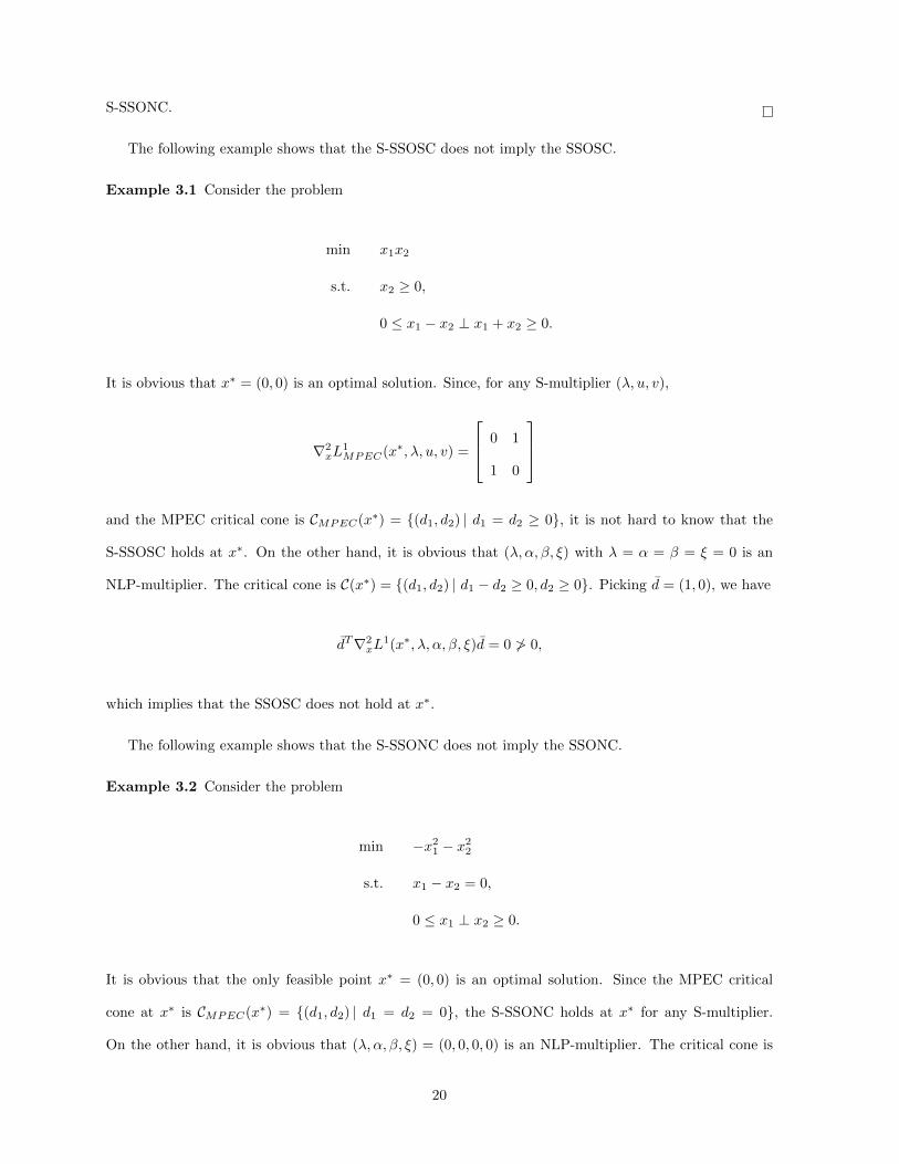
The following example shows that the S-SSOSC does not imply the SSOSC.
Example 3.1 Consider the problem
min x1x2
s.t. x2 ≥ 0,
0 ≤ x1 − x2 ⊥ x1 + x2 ≥ 0.
It is obvious that x∗ = (0, 0) is an optimal solution. Since, for any S-multiplier (λ, u, v),
∇2xL
1MPEC(x∗, λ, u, v) =
0 1
1 0
and the MPEC critical cone is CMPEC(x∗) = (d1, d2) | d1 = d2 ≥ 0, it is not hard to know that the
S-SSOSC holds at x∗. On the other hand, it is obvious that (λ, α, β, ξ) with λ = α = β = ξ = 0 is an
NLP-multiplier. The critical cone is C(x∗) = (d1, d2) | d1 − d2 ≥ 0, d2 ≥ 0. Picking d = (1, 0), we have
dT∇2xL
1(x∗, λ, α, β, ξ)d = 0 ≯ 0,
which implies that the SSOSC does not hold at x∗.
The following example shows that the S-SSONC does not imply the SSONC.
Example 3.2 Consider the problem
min −x21 − x2
2
s.t. x1 − x2 = 0,
0 ≤ x1 ⊥ x2 ≥ 0.
It is obvious that the only feasible point x∗ = (0, 0) is an optimal solution. Since the MPEC critical
cone at x∗ is CMPEC(x∗) = (d1, d2) | d1 = d2 = 0, the S-SSONC holds at x∗ for any S-multiplier.
On the other hand, it is obvious that (λ, α, β, ξ) = (0, 0, 0, 0) is an NLP-multiplier. The critical cone is
20
C(x∗) = (d1, d2) | d1 = d2 ≥ 0. Picking d = (1, 1), we have
dT∇2xL
1(x∗, λ, α, β, ξ)d = −4 < 0,
which implies that the SSONC does not hold at x∗.
Scheel and Scholtes [2, Theorem 7 (2)] showed that the S-RSOSC at a feasible point with r = 1
implies that the point is a strict local minimizer. In what follows, we show that the second-order sufficient
condition in terms of either the S-multiplier or the singular S-multiplier provides a useful information for
local optimality. This is very interesting for MPEC since singular S-multipliers always exist.
Theorem 3.2 Let x∗ ∈ X. If the S-RSOSC holds at x∗, then there exist δ > 0 and c > 0 such that
f(x) ≥ f(x∗) + c‖x− x∗‖2, ∀x ∈ X ∩ Bδ(x∗).
Proof. By Corollary 3.1, the S-RSOSC holds at x∗ if and only if the RSOSC holds at x∗. The conclusion
follows from Proposition 2.1 immediately.
In order to study second-order necessary optimality conditions for MPEC, we next extend various
relaxations of LICQ for (1) in Definition 2.2 to the MPEC (5). All these conditions are weaker than
the MPEC-LICQ and MPEC Linear CQ. The latter means that all constraint functions are affine [4].
The MPEC-CRCQ has been studied to analyze convergence of relaxation methods for solving MPEC
in [45,46]. The other weaker constraint qualifications may be also useful in convergence analysis.
Definition 3.4 Let x∗ ∈ X.
(i) We say that the MPEC constant rank constraint qualification (MPEC-CRCQ) is satisfied at x∗ iff
there exists δ > 0 such that, for any I1 ⊆ I∗g , I2 ⊆ 1, · · · , q, I3 ⊆ I∗ ∪ J ∗, and I4 ⊆ K∗ ∪ J ∗,
the family of gradients
∇gi(x),∇hj(x),∇Gı(x),∇H(x)
∣∣ i ∈ I1, j ∈ I2, ı ∈ I3, ∈ I4
has the same rank for each x ∈ Bδ(x∗).
(ii) We say that the MPEC relaxed constant rank constraint qualification (MPEC-RCRCQ) is satisfied
21
at x∗ iff there exists δ > 0 such that, for any I1 ⊆ I∗g and I2, I3 ⊆ J ∗, the family of gradients
∇gi(x),∇hj(x),∇Gı(x),∇H(x)
∣∣ i ∈ I1, j = 1, · · · , q, ı ∈ I∗ ∪ I2, ∈ K∗ ∪ I3
has the same rank for each x ∈ Bδ(x∗).
(iii) We say that the MPEC weak relaxed constant rank condition (MPEC-WRCR) is satisfied at x∗ iff
there exists δ > 0 such that, for any I ⊆ I∗g , the family of gradients
∇gi(x),∇hj(x),∇Gı(x),∇H(x)
∣∣ i ∈ I, j = 1, · · · , q, ı ∈ I∗ ∪ J ∗, ∈ K∗ ∪ J ∗
has the same rank for each x ∈ Bδ(x∗).
(iv) We say that the MPEC weak constant rank condition (MPEC-WCR) is satisfied at x∗ iff there
exists δ > 0 such that the family of gradients
∇gi(x),∇hj(x),∇Gı(x),∇H(x)
∣∣ i ∈ I∗g , j = 1, · · · , q, ı ∈ I∗ ∪ J ∗, ∈ K∗ ∪ J ∗
has the same rank for each x ∈ Bδ(x∗).
We are ready to study the second-order necessary conditions for MPEC. To this end, we introduce
two sets. For any y∗ ∈M1C(x∗), define
X :=
x
∣∣∣∣∣∣∣∣∣∣∣∣∣∣
gi(x) = 0 if i ∈ I∗g and λ∗i > 0, gi(x) ≤ 0 if i ∈ I∗g and λ∗i = 0
hi(x) = 0 for i = 1, · · · , q, Gi(x) = 0 if i ∈ I∗, Hi(x) = 0 if i ∈ K∗
Gi(x) = 0 if i ∈ J ∗ and u∗i 6= 0, Hi(x) = 0 if i ∈ J ∗ and v∗i 6= 0,
0 ≤ Gi(x) ⊥ Hi(x) ≥ 0 if i ∈ J ∗
.
22

Its linearized cone at x∗ is given by
C(x∗) =
d
∣∣∣∣∣∣∣∣∣∣∣∣∣∣∣∣∣∣
∇gi(x∗)T d = 0 if i ∈ I∗g and λ∗i > 0, ∇gi(x∗)T d ≤ 0 if i ∈ I∗g and λ∗i = 0
∇hi(x∗)T d = 0 for i = 1, 2, · · · , q
∇Gi(x∗)T d = 0 if i ∈ I∗, ∇Hi(x∗)T d = 0 if i ∈ K∗
∇Gi(x∗)T d = 0 if i ∈ J ∗ and u∗i 6= 0, ∇Hi(x∗)T d = 0 if i ∈ J ∗ and v∗i 6= 0,
0 ≤ ∇Gi(x∗)T d ⊥ ∇Hi(x∗)T d ≥ 0 if i ∈ J ∗
.
It is easy to see that X is a subset of the feasible region X locally around x∗. In the case of nonlinear
programs, C(x∗) is equal to the classical critical cone. The following second-order condition holds without
any constraint qualification.
Theorem 3.3 Let x∗ be a locally optimal solution of (5) and y∗ ∈M1C(x∗). Then
dT∇2xL
1MPEC(x∗, y∗)d ≥ 0, ∀d ∈ TX(x∗).
Proof. Let d ∈ TX(x∗). By definition, there exist tk ≥ 0 and xk →X x∗ such that limk→∞
tk(xk−x∗) = d.
By the Taylor series expansion, we have
L1MPEC(xk, y∗) = L1
MPEC(x∗, y∗) +∇xL1MPEC(x∗, y∗)T (xk − x∗)
+1
2(xk − x∗)T∇2
xL1MPEC(x∗, y∗)(xk − x∗) + o(‖xk − x∗‖2). (14)
Since xk ∈ X and y∗ ∈ M1C(x∗), we have L1
MPEC(xk, y∗) = f(xk), ∇xL1MPEC(x∗, y∗) = 0, and
L1MPEC(x∗, y∗) = f(x∗). Thus, we have from (14) that
f(xk) = f(x∗) +1
2(xk − x∗)T∇2
xL1MPEC(x∗, y∗)(xk − x∗) + o(‖xk − x∗‖2). (15)
Since xk ∈ X for each k sufficiently large and x∗ is locally optimal, we have f(xk) ≥ f(x∗) when k is
sufficiently large. Thus, it follows from (15) that
(xk − x∗)T∇2xL
1MPEC(x∗, y∗)(xk − x∗) + o(‖xk − x∗‖2) ≥ 0.
23
Multiplying it by t2k and taking a limit, we get the desired result.
As a consequence, we have the following strong second-order necessary optimality condition.
Corollary 3.2 Let x∗ be a locally optimal solution of (5) and y∗ ∈ M1C(x∗). If the Abadie CQ for X
holds at x∗, i.e., C(x∗) ⊆ TX(x∗), then
dT∇2xL
1MPEC(x∗, y∗)d ≥ 0, ∀d ∈ C(x∗).
We now investigate the conditions under which C(x∗) ⊆ TX(x∗) holds.
The following result shows that the MPEC-RCRCQ is a constraint qualification for M-stationarity.
Lemma 3.1 Suppose that the MPEC-RCRCQ holds at x∗ ∈ X. Then the MPEC Abadie CQ holds at
x∗, i.e., TX(x∗) = LMPEC(x∗).
Proof. Let P(J ∗) := (J ∗1 ,J ∗2 ) | J ∗1 ∪ J ∗2 = J ∗,J ∗1 ∩ J ∗2 = ∅. For each partition (J ∗1 ,J ∗2 ) ∈ P(J ∗),
we consider the following restricted problem associated with (5):
min f(x)
s.t. g(x) ≤ 0, h(x) = 0,
GI∗∪J ∗1
(x) = 0, GJ ∗2
(x) ≥ 0,
HK∗∪J ∗2
(x) = 0, GJ ∗1
(x) ≥ 0.
(16)
Denote by X(J ∗1 ,J ∗2 ) the feasible region of (16). It is not difficult to see that
TX(x∗) =⋃
(J ∗1 ,J ∗
2 )∈P(J ∗)
TX(J ∗1 ,J ∗
2 )(x∗), LMPEC(x∗) =
⋃(J ∗
1 ,J ∗2 )∈P(J ∗)
LX(J ∗1 ,J ∗
2 )(x∗), (17)
where LX(J ∗1 ,J ∗
2 )(x∗) is the linearized tangent cone of X(J ∗1 ,J ∗2 ) at x∗.
Since x∗ satisfies the MPEC-RCRCQ, the RCRCQ holds at x∗ ∈ X(J ∗1 ,J ∗2 ) for each partition
(J ∗1 ,J ∗2 ) ∈ P(J ∗). Since the RCRCQ implies the RCPLD, it follows from Lemma 2.1 that
TX(J ∗1 ,J ∗
2 )(x∗) = LX(J ∗
1 ,J ∗2 )(x
∗), ∀(J ∗1 ,J ∗2 ) ∈ P(J ∗).
This, together with (17), implies TX(x∗) = LMPEC(x∗).
24
Theorem 3.4 If the MPEC-RCRCQ holds at x∗ ∈ X and y∗ ∈M1C(x∗), then C(x∗) ⊆ TX(x∗).
Proof. Since the MPEC-RCRCQ holds at x∗ ∈ X, the MPEC-RCRCQ holds at x∗ ∈ X. It follows
from Lemma 3.1 that C(x∗) ⊆ TX(x∗).
Now we are ready to show that, under the MPEC-RCRCQ, any locally optimal solution satisfies the
S-SSONC. This result improves the result of Scheel and Scholtes [2, Theorem 7 (1)], who proved the
S-RSONC (weaker than the S-SSONC) under the MPEC SMFCQ (stronger than the MPEC-RCRCQ).
Theorem 3.5 Suppose that x∗ is a locally optimal solution of (5) and the MPEC-RCRCQ holds at x∗.
Then M1M (x∗) 6= ∅ and, for any y∗ ∈M1
S(x∗),
dT∇2xL
1MPEC(x∗, y∗)d ≥ 0, ∀d ∈ CMPEC(x∗).
Proof. By Lemma 3.1, we have TX(x∗) = LMPEC(x∗) and then, by [4, Theorem 3.1], M1M (x∗) 6= ∅.
Let y∗ ∈ M1S(x∗). By Theorem 3.4, we have C(x∗) = TX(x∗). By virtue of Corollary 3.2, it suffices to
show that CMPEC(x∗) ⊆ C(x∗). In fact, for any d ∈ CMPEC(x∗), by definition of MPEC critical cone, we
have ∇f(x∗)T d ≤ 0 and d ∈ LMPEC(x∗). On the other hand, by the local optimality of x∗, we have
∇f(x∗)T d ≥ 0, ∀d ∈ TX(x∗) = LMPEC(x∗).
It follows that ∇f(x∗)T d = 0. Thus, we have from (11) that d ∈ C(x∗).
Theorem 3.6 Let x∗ be a locally optimal solution of the MPEC (5). If the MPEC-WRCR condition
holds at x∗, then, for any y∗ ∈M1C(x∗), we have
dT∇2xL
1MPEC(x∗, y∗)d ≥ 0, ∀d ∈ C(x∗),
where
C(x∗) :=
d
∣∣∣∣∣∣∣∣∣∣∣∣∣∣
∇gi(x∗)T d = 0 if i ∈ I∗g and λ∗i > 0
∇gi(x∗)T d ≤ 0 if i ∈ I∗g and λ∗i = 0
∇hi(x∗)T d = 0 for i = 1, · · · , q
∇Gi(x∗)T d = 0 if i ∈ I∗ ∪ J ∗, ∇Hi(x∗)T d = 0 if i ∈ K∗ ∪ J ∗
.
25

Proof. Consider the set
X :=
x
∣∣∣∣∣∣∣∣∣∣∣gi(x) = 0 if i ∈ I∗g and λ∗i > 0, gi(x) ≤ 0 if i ∈ I∗g and λ∗i = 0
hi(x) = 0 for i = 1, · · · , q
Gi(x) = 0 if i ∈ I∗ ∪ J ∗, Hi(x) = 0 if i ∈ K∗ ∪ J ∗
.
Since the MPEC-WRCR condition holds at x∗, the RCRCQ holds at x∗ for X. Thus, we have from
Lemma 2.1 that
TX(x∗) = C(x∗).
Therefore, the desired result can be obtained from Theorem 3.3 and TX(x∗) ⊆ TX(x∗).
The second-order necessary condition given in Theorem 3.6 is reasonable because the cone C(x∗) is
actually the critical cone of the following tightened problem associated with (5):
min f(x)
s.t. g(x) ≤ 0, h(x) = 0,
GI∗∪J ∗(x) = 0, HK∗∪J ∗(x) = 0.
(18)
Theorem 3.7 Let x∗ be a locally optimal solution of the MPEC (5). If the MPEC-WCR condition holds
at x∗, then, for any y∗ ∈M1C(x∗), we have
dT∇2xL
1MPEC(x∗, y∗)d ≥ 0, ∀d ∈ CMPEC(x∗).
Proof. Consider the set
X :=
x∣∣∣∣∣∣∣gi(x) = 0, if i ∈ I∗g , hi(x) = 0 for i = 1, · · · , q
Gi(x) = 0 if i ∈ I∗ ∪ J ∗, Hi(x) = 0 if i ∈ K∗ ∪ J ∗
.
Since the MPEC-WCR condition holds at x∗, the RCRCQ holds at x∗ for X. Thus, we have from Lemma
2.1 that
TX(x∗) = CMPEC(x∗).
Therefore, the desired result can be obtained from Theorem 3.3 and TX(x∗) ⊆ TX(x∗).
26

Note that the cone CMPEC(x∗) defined in Theorem 3.7 is independent of the objective function of (5).
We close this section by illustrating that both C(x∗) ⊆ TX(x∗) and the MPEC Abadie CQ are strictly
weaker than the MPEC-RCRCQ and, moreover, the MPEC-WRCR and the MPEC-WCR imply neither
C(x∗) ⊆ TX(x∗) nor the MPEC Abadie CQ, and neither of them is a constraint qualification for the
M-stationarity.
The following example shows that C(x) ⊆ TX(x) and the MPEC Abadie CQ hold at some point x,
but the MPEC-RCRCQ does not hold at x.
Example 3.3 Consider the problem
min f(x1, x2) ≡ 1
s.t. x2 ≤ 0, −x1 + x22 ≤ 0,
0 ≤ x1 ⊥ x2 ≥ 0.
It is obvious that every feasible point is a globally optimal solution. Take x := (0, 0). Since
( 10 ) ,( −1
2x2
)has rank one when x = x and rank two when x2 6= x2, the MPEC-RCRCQ does not hold at x. Denote
by X the feasible region of the problem. It is not hard to show that (0, 0; 0, 0, 0, 0) is an S-stationary pair
for the problem and X = X. It is easy to verify that TX(x) = C(x) = (d1, d2) | d1 ≥ 0, d2 = 0 and
TX(x) = LMPEC(x).
The following example shows that both the MPEC-WRCR and MPEC-WCR hold at some point x,
but C(x) ⊆ TX(x) and the MPEC Abadie CQ do not hold at x.
Example 3.4 Consider the problem
min f(x1, x2) ≡ 1
s.t. x2 − x21 = 0,
0 ≤ −x1 ⊥ x2 ≥ 0.
It is obvious that the only feasible point is x := (0, 0). Since(−2x1
1
),(−1
0
), ( 0
1 )
has rank two for
any x, both the MPEC-WRCR and the MPEC-WCR hold at x. Denote by X the feasible region of the
problem. It is not hard to see that (0, 0; 1, 0, 1) is an S-stationary pair of the problem and X = X. By
27

direct calculation, we can get TX(x) = 0 and C(x) = (d1, d2) | d1 ≤ 0, d2 = 0. Thus, C(x) * TX(x).
Moreover, TX(x) = 0 and LMPEC(x) = (d1, d2) | d1 ≤ 0, d2 = 0, which means that the MPEC
Abadie CQ does not holds at x.
The following example, which originates from [17, Example 2.2], shows that both the MPEC-WRCR
and MPEC-WCR are not constraint qualifications for M-stationarity.
Example 3.5 Consider the problem
min x1 + x2 − x3 −1
2x4
s.t. x24 = 0, (19)
−6x1 + x3 + x4 = 0, −6x2 + x3 = 0,
0 ≤ x1 ⊥ x2 ≥ 0.
It is obvious that the unique feasible point x = (0, 0, 0, 0) is a global solution. Moreover, it is not hard
to see that the MPEC-WRCR and MPEC-WCR hold at x. By solving the M-stationarity conditions, we
can obtain that the multipliers corresponding to J ∗ is u = v = −2. Since u < 0 and v < 0, the unique
minimizer (0, 0, 0, 0) is not an M-stationary point.
4 Isolatedness of Local Minimizers
In this section, we investigate conditions under which an M- or S-stationary point of the MPEC (5) must
be an isolated local minimizer. Theorem 3.2 shows that any feasible point satisfying the S-RSOSC is
locally optimal. However, the following example, which originates from [39], shows that an S-stationary
point satisfying the S-SSOSC (stronger than the S-RSOSC) may not be an isolated local minimizer. To
ensure a stationary point to be isolated, some constraint qualification is required.
Example 4.1 Consider the problem
min1
2(x2 + y2)
s.t. h(x) = 0,
0 ≤ x ⊥ y ≥ 0,
28

where
h(x) :=
x5 sin 1
x , x 6= 0,
0, x = 0.
The feasible region is (0, y) | y ≥ 0∪( 1kπ , 0) | k = 1, 2, · · · . It is not difficult to verify that every point
of the set ( 1kπ , 0) | k = 0, 1, 2, · · · is both locally optimal and S-stationary, and the S-RSOSC holds at
(0, 0). However, (0, 0) is neither an isolated locally optimal solution nor an isolated S-stationary point.
Definition 4.1 We say that the M-multiplier strong second-order sufficient condition (M-SSOSC) holds
at x∗ ∈ X iff, for every y∗ ∈M1M (x∗),
dT∇2xL
1MPEC(x∗, y∗)d > 0, ∀d ∈ CMPEC(x∗)\0.
Recently, the CPLD for nonlinear programs in Definition 2.3 was extended to MPEC in [45] and [7],
respectively. Note that the constraint qualification in the sense of [7] is weaker than the one in the sense
of [45].
Definition 4.2 [7] We say that the MPEC constant positive linear dependent condition (MPEC-CPLD)
holds at x∗ ∈ X iff, for any I1 ⊆ I∗g , I2 ⊆ 1, · · · , q, I3 ⊆ I∗ ∪ J ∗ and I4 ⊆ K∗ ∪ J ∗, whenever there
exist multipliers, not all zero, λ, µ, u, v with λi ≥ 0 for each i ∈ I1, either ulvl = 0 or ul > 0, vl > 0 for
each l ∈ J ∗, such that
∑i∈I1
λi∇gi(x∗) +∑j∈I2
µj∇hj(x∗)−∑l∈I3
ul∇Gl(x∗)−∑l∈I4
vl∇Hl(x∗) = 0,
there exists a neighborhood B(x∗) of x∗ such that, for any x ∈ B(x∗), the vectors
∇hi(x)| i ∈ I1, ∇gj(x)| j ∈ I2, ∇Gl(x)| l ∈ I3, ∇Hl(x)| l ∈ I4
are linearly dependent.
The MPEC-CPLD is obviously weaker than the MPEC NNAMCQ and MPEC-CRCQ. Motivated
by the RCPLD in [33], we define an MPEC-type RCPLD, which is weaker than the MPEC-CPLD and
29
MPEC-RCRCQ. Given a point x and three index sets I1 ⊆ 1, · · · , q and I2, I3 ⊆ 1, · · · ,m, we denote
G(x; I1, I2, I3) := ∇hj(x),∇Gı(x),∇H(x) | j ∈ I1, ı ∈ I2, ∈ I3.
Definition 4.3 Let I1 ⊆ 1, · · · , q, I2 ⊆ I∗, and I3 ⊆ K∗ be such that G(x∗; I1, I2, I3) is a basis for the
generated space spanG(x∗; 1, · · · , q, I∗,K∗). We say that the MPEC-relaxed constant positive linear
dependence (MPEC-RCPLD) holds at x∗ iff there exists δ > 0 such that
– G(x; 1, · · · , q, I∗,K∗) has the same rank for each x ∈ Bδ(x∗);
– for each I4 ⊆ I∗g and I5, I6 ⊆ J ∗, whenever there exist multipliers, not all zero, λ, µ, u, v with
λi ≥ 0 for each i ∈ I4, either ulvl = 0 or ul > 0, vl > 0 for each l ∈ J ∗, such that
∑i∈I4
λi∇gi(x∗) +∑j∈I1
µj∇hj(x∗)−∑
ı∈I2∪I5
uı∇Gı(x∗)−∑
∈I3∪I6
v∇H(x∗) = 0,
then, for any x ∈ Bδ(x∗), the vectors
∇gi(x)| i ∈ I4, ∇hj(x)| j ∈ I1, ∇Gı(x)| ı ∈ I2 ∪ I5, ∇H(x)| ∈ I3 ∪ I6
are linearly dependent.
The MPEC-RCPLD has been shown to be a constraint qualification for M-stationarity in [47]. In
the case where there is no complementarity constraint, the MPEC-RCPLD reduces to the relaxed
constant positive linear dependence (RCPLD) condition introduced recently in [33] for standard
nonlinear programs.
The following result can be seen as a corollary of Caratheodory’s lemma [48].
Lemma 4.1 [33] If x =∑m+pi=1 αivi with vi | i = 1, · · · ,m to be linearly independent and αi 6= 0 for
i = m + 1, · · · ,m + p, then there exist J ⊆ m + 1, · · · ,m + p and αi for i ∈ 1, · · · ,m ∪ J such
that x =∑i∈1,··· ,m∪J αivi with αiαi > 0 for every i ∈ J and vi |ı ∈ 1, · · · ,m ∪ J is linearly
independent.
Theorem 4.1 Let x∗ be an M-stationary point of the MPEC (5). Suppose that both the MPEC-RCPLD
and M-SSOSC hold at x∗. Then there exists a constant δ > 0 such that, if x ∈ Bδ(x∗) ∩ X and (x, y)
30

satisfies (10) for some y, there must hold x = x∗.
Proof. Suppose to the contrary that there exist a sequence xk ⊆ X\x∗ converging to x∗ and an
associated multiplier sequence yk satisfying
0 = ∇f(xk) +∇F (xk)yk,
yk ∈ NΛ(F (xk)).
(20)
We first show that there exists a bounded subsequence ykk∈K satisfying (20). Assume that
∇f(xk) 6= 0 for each k (otherwise, we can choose a subsequence and redefine yk = 0 for each k ∈ K,
which is obviously bounded and satisfies (20)). For sake of convenience, denote
Ikg := i | gi(xk) = 0,
Ik := i | Gi(xk) = 0 < Hi(xk),
J k := i | Gi(xk) = 0 = Hi(xk),
Kk := i | Gi(xk) > 0 = Hi(xk).
Since I∗ ⊆ Ik and K∗ ⊆ Kk for each k sufficiently large, it follows from the first equality in (20) that
0 = ∇f(xk) +
q∑i=1
µki∇hi(xk)−∑ı∈I∗
ukı∇Gı(xk)−∑∈K∗
vk∇H(xk)−
∑ı∈Ik\I∗∪J k∩supp(uk)
ukı∇Gı(xk)−∑
∈Kk\K∗∪J k∩supp(vk)
vk∇H(xk) +
∑j∈supp(λk)
λkj∇gj(xk),
(21)
where supp(a) := i | ai 6= 0. Let I1 ⊆ 1, · · · , q, I2 ⊆ I∗, and I3 ⊆ K∗ be such that G(x∗; I1, I2, I3) is
a basis for spanG(x∗; 1, · · · , q, I∗,K∗). Then G(xk; I1, I2, I3) is linearly independent for k sufficiently
large. Since there is a constant δ > 0 such that the rank of G(x; 1, · · · , q, I∗,K∗) is constant for each
x ∈ Bδ(x∗), we have that G(xk; I1, I2, I3) is a basis for
spanG(xk; 1, · · · , q, I∗,K∗)
31

for k sufficiently large. Thus, it follows from (21) and Lemma 4.1 that there exist Ik4 ⊆ supp(λk),
Ik5 ⊆ Ik \ I∗ ∪ J k ∩ supp(uk), Ik6 ⊆ Kk \ K∗ ∪ J k ∩ supp(vk), and µk, λk, uk, and vk such that
0 = ∇f(xk) +∑i∈I1
µki∇hi(xk)−∑ı∈I2
ukı∇Gı(xk)−∑∈I3
vk∇H(xk)
+∑j∈Ik4
λkj∇gj(xk)−∑ı∈Ik5
ukı∇Gı(xk)−∑∈Ik6
vk∇Hı(xk),
and
∇gj(xk) | j ∈ Ik4 , ∇hi(xk) | i ∈ I1, ∇Gı(xk) | ı ∈ I2 ∪ Ik5 , ∇H(xk) | ∈ I3 ∪ Ik6
are linearly independent for k sufficiently large. Set λki = 0 for i /∈ Ik4 , µki = 0 for i /∈ I1, and ukı = 0
for ı /∈ I2 ∪ Ik5 , vk = 0 for /∈ I3 ∪ Ik6 . It is not hard from the above process and Lemma 4.1 that
(λk, µk, uk, vk) ∈ M1M (xk). Without any loss of generality, we assume that Ik4 ≡ I4, Ik5 ≡ I5, and
Ik6 ≡ I6. Then
∇gj(xk) | j ∈ I4, ∇hi(xk) | i ∈ I1, ∇Gı(xk) | ı ∈ I2 ∪ I5, ∇H(xk) | ∈ I3 ∪ I6 (22)
are linearly independent. It is not hard to get that I4 ⊆ I∗g , I1 ⊆ 1, · · · , q, and I5, I6 ∈ J ∗ by
Ik ∪ J k ∪ Kk = I∗ ∪ J ∗ ∪ K∗. Assume that yk = (λk, µk, uk, vk) is unbounded and, without any loss of
generality, yk/‖yk‖ → y∗ with ‖y∗‖ = 1. Since yk = (λk, µk, uk, vk) ∈M1M (x∗), we have
0 = ∇f(xk) +∇F (xk)yk,
yk ∈ NΛ(F (xk)).
Thus, we have from the outer semicontinuity of NΛ (see, e.g., [44, Proposition 6.6]) that
0 = limk→∞
(∇xf(xk)
‖yk‖+∇xF (xk)yk
‖yk‖
)= ∇xF (x∗)y∗,
y∗ = limk→∞
yk
‖yk‖∈ lim sup
k→∞NΛ(F (xk)) = NΛ(F (x∗)).
Thus, we have 0 6= y∗ = (λ∗, µ∗, u∗, v∗) ∈M1M (x∗) and
∑i∈I4
λ∗i∇gi(x∗) +∑j∈I1
µ∗j∇hj(x∗)−∑
ı∈I2∪I5
u∗ı∇Gı(x∗)−∑
∈I3∪I6
v∗∇H(x∗) = 0.
32

Clearly, λ∗i ≥ 0 for i ∈ I4 and either u∗l v∗l = 0 or u∗l > 0, v∗l > 0 for l ∈ J ∗ . This, together with
(22), contradicts the MPEC-RCPLD assumption at x∗. Thus, ykk∈K is bounded. Without any loss
of generality, we may assume that yk is a bounded sequence satisfying (20). We may further assume
that yk → y∗. Clearly, from the outer semicontinuity of NΛ, y∗ ∈ NΛ(F (x∗)) and hence y∗ ∈ M1M (x∗).
Assume further that (xk − x∗)/‖xk − x∗‖ → d0 with ‖d0‖ = 1. Note that, for each k,
Λ 3 F (xk) = F (x∗) +∇F (x∗)T (xk − x∗) + o(‖xk − x∗‖),
and hence
∇F (x∗)T d0 = limk→∞
F (xk)− F (x∗)
‖xk − x∗‖∈ TΛ(F (x∗)). (23)
It follows from (20) and [44, Proposition 6.41] that
yk ∈l∏i=1
N(−∞,0](gi(xk))×
q∏i=1
N0(hi(xk))×m∏i=1
NC(−Gi(xk),−Hi(xk)). (24)
It follows from (24) and Proposition 3.1 that, for each j
ykj Fj(xk) = 0. (25)
We next show that (yk)TF (x∗) = (y∗)TF (xk) = 0 for each k sufficiently large. In fact, if Fj(x∗) 6= 0
for some j, then Fj(xk) 6= 0 when k is sufficiently large and hence, by (25), ykj = 0. As a result, we
always have (yk)TF (x∗) = 0. We can show (y∗)TF (xk) = 0 when k is sufficiently large in a similar way.
Therefore, we have that, for each k sufficiently large,
(yk)TF (x∗) = (y∗)TF (xk) = (yk)TF (xk) = 0. (26)
33

Noting that yk is bounded, we have that, for each k sufficiently large,
0 = (yk)TF (xk)
= (yk)TF (x∗) + (yk)T∇F (x∗)T (xk − x∗) + o(‖xk − x∗‖)
= (yk)T∇F (x∗)T (xk − x∗) + o(‖xk − x∗‖).
Dividing it by ‖xk − x∗‖ and taking a limit, we obtain
(y∗)T∇F (x∗)T d0 = 0.
It follows from (20) that
0 = ∇f(xk)T (xk − x∗) + (yk)T∇F (xk)T (xk − x∗). (27)
Dividing it by ‖xk − x∗‖ and taking a limit, we have ∇f(x∗)T d0 = 0. This, together with (23), indicates
d0 ∈ CMPEC(x∗) and then, by the M-SSOSC assumption,
(d0)T∇2xL
1MPEC(x∗, y∗)d0 > 0. (28)
Let k be large enough. Consider the smooth function sk defined by
sk(t) := (∇f(xt) +∇F (xt)yt)T (xk − x∗)− F (xt)
T (yk − y∗),
where (xt, yt) := (1− t)(x∗, y∗) + t(xk, yk). It is not difficult to see from (10) and (20) that the first term
vanishes when t = 0 or t = 1. On the other hand,
• if t = 0, it follows from (26) and y∗ ∈ NΛ(F (x∗)) that
F (xt)T (yk − y∗) = F (x∗)T (yk − y∗) = 0;
34

• if t = 1, it follows from (26) that
F (xt)T (yk − y∗) = F (xk)T yk − F (xk)T y∗ = 0.
As a result, we have sk(0) = 0 = sk(1). By the mean value theorem, there exists tk ∈ (0, 1) such that
0 = s′k(tk) = (xk − x∗)T∇2xL
1MPEC(xtk , ytk)(xk − x∗).
Dividing it by ‖xk−x∗‖2 and taking a limit, we obtain a contradiction to (28). This completes the proof.
We can get the following isolatedness result of S-stationary point immediately. Due to the fact that
a limit point of S-stationary points may not be S-stationary, we do not know whether the M-SSOSC can
be weakened to the S-SSOSC.
Corollary 4.1 Let x∗ be an S-stationary point of the MPEC (5). Suppose that both the MPEC-RCPLD
and M-SSOSC hold at x∗. Then there exists a neighborhood V of x∗ containing no other S-stationary
point.
Theorem 4.2 If the MPEC-CPLD holds at x∗ ∈ X, there exists δ > 0 such that, for each x ∈ Bδ(x∗)∩X,
the MPEC-CPLD holds at x.
Proof. Assume to the contrary that there exists a sequence xk →X x∗ such that the MPEC-CPLD
does not hold at xk for each k. That is, for each k, there exist index sets Ik1 ⊆ Ikg , Ik2 ⊆ 1, · · · , q,
Ik3 ⊆ Ik∪J k, and Ik4 ⊆ Kk∪J k, where Ikg , Ik,J k,Kk are the same as in the proof of Theorem 20, and
multipliers, not all zero, λk, µk, uk, vk with λki ≥ 0 for each i ∈ Ik1 , either ukl vkl = 0 or ukl > 0, vkl > 0
for each l ∈ J k such that
∑i∈Ik1
λki∇gi(xk) +∑j∈Ik2
µkj∇hj(xk)−∑l∈Ik3
ukl∇Gl(xk)−∑l∈Ik4
vkl ∇Hl(xk) = 0, (29)
and there exists sequence yk,ν converging to xk as ν →∞ such that
∇gi(yk,ν),∇hj(yk,ν),∇Gl(yk,ν),∇H(y
k,ν)∣∣ i ∈ Ik1 , j ∈ Ik2 , l ∈ Ik3 , ∈ Ik4 (30)
35

is linearly independent. Without any loss of generality, we may assume that Ik1 ≡ I1, Ik2 ≡ I2, Ik3 ≡ I3,
and Ik4 ≡ I4. It is not difficult to get that I1 ⊆ I∗g , I2 ⊆ 1, · · · , q, I3 ⊆ I∗ ∪ J ∗, and I4 ⊆ K∗ ∪ J ∗.
Set λki = 0 for i /∈ I1, uki = 0 for i /∈ I3, and vki = 0 for i /∈ I4. We may further assume that
(λk, µk, uk, vk)/‖(λk, µk, uk, vk)‖ → (λ∗, µ∗, u∗, v∗) with (λ∗, µ∗, u∗, v∗) = 1. Dividing (29) by
‖(λk, µk, uk, vk)‖ and taking a limit in (29), we have
∑i∈I1
λ∗i∇gi(x∗) +∑j∈I2
µ∗j∇hj(x∗)−∑l∈I3
u∗l∇Gl(x∗)−∑l∈I4
v∗l∇Hl(x∗) = 0. (31)
It is not hard to get from (29) and Proposition 3.1 that
yk = (λk, µk, uk, vk)/‖(λk, µk, uk, vk)‖ ∈ NΛ(F (xk)).
Therefore, we have from the outer semicontinuity of NΛ that y∗ ∈ NΛ(F (x∗)). Thus, we have from
Proposition 3.1 that
either u∗l v∗l = 0 or u∗l > 0, v∗l > 0 for each l ∈ J ∗. (32)
By the diagonalization law, we have from (30) that there exists zk → x∗ such that
∇gi(zk),∇hj(zk),∇Gl(zk),∇H(z
k)∣∣ i ∈ I1, j ∈ I2, l ∈ I3, ∈ I4
is linearly independent, which together with (31)–(32) gives a contradiction with the assumption that the
MPEC-CPLD holds at x∗. This completes the proof.
Corollary 4.2 Let x∗ be an M-stationary point of the MPEC (5). Suppose that both MPEC-CPLD and
M-SSOSC hold at x∗. Then there exists a neighborhood V of x∗ such that x∗ is the only possibly local
minimizer of the MPEC (5) in V ∩X. If, in addition, x∗ is an S-stationary point of (5), then x∗ is the
only local minimizer of the MPEC (5)in V ∩X.
Proof. Let V1 be the open neighborhood in Theorem 4.1 such that there is no other M-stationary point
in V1 ∩X and V2 be the open neighborhood in Theorem 4.2 such that the MPEC-CPLD holds at each
element in V2 ∩ X. Set V := V1 ∩ V2. Since any locally optimal solution satisfying the MPEC-CPLD
36
must be M-stationary [7], the set V is the required one. The rest of the theorem follows from Theorem
3.2.
We further have the following result from Theorem 3.2 and Corollary 4.2. Note that the M-SSOSC
for the MPEC (5) with linear constraints is independent of M-multipliers.
Corollary 4.3 Suppose that F is affine and x∗ is an S-stationary point of (5). Let the M-SSOSC hold
at x∗. Then there exists a neighborhood V of x∗ containing no other local minimizer of (5).
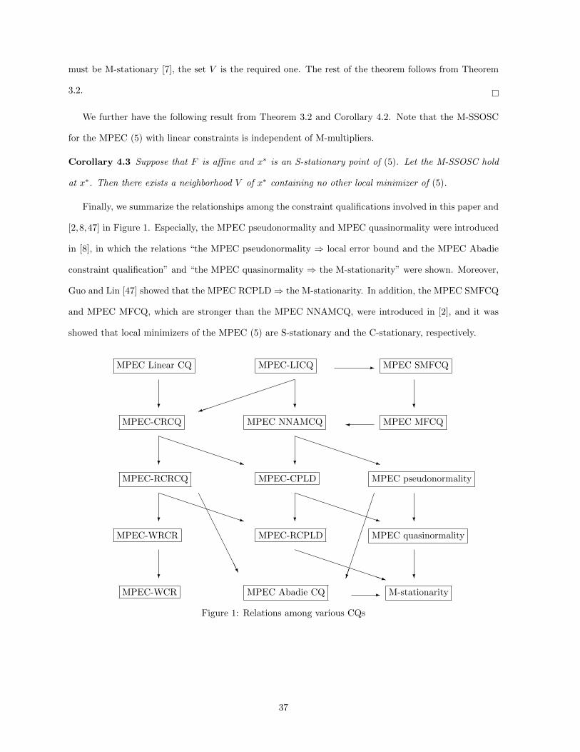
Finally, we summarize the relationships among the constraint qualifications involved in this paper and
[2,8,47] in Figure 1. Especially, the MPEC pseudonormality and MPEC quasinormality were introduced
in [8], in which the relations “the MPEC pseudonormality ⇒ local error bound and the MPEC Abadie
constraint qualification” and “the MPEC quasinormality ⇒ the M-stationarity” were shown. Moreover,
Guo and Lin [47] showed that the MPEC RCPLD⇒ the M-stationarity. In addition, the MPEC SMFCQ
and MPEC MFCQ, which are stronger than the MPEC NNAMCQ, were introduced in [2], and it was
showed that local minimizers of the MPEC (5) are S-stationary and the C-stationary, respectively.
MPEC-LICQMPEC Linear CQ MPEC SMFCQ
?
MPEC MFCQ
-
?
)?
MPEC NNAMCQ
PPPPPPPPPq
MPEC-CRCQ
?
PPPPPPPPPq
MPEC-RCRCQ
PPPPPPPPPq ?
MPEC-WRCR
?
MPEC-WCR
?
MPEC-CPLD
PPPPPPPPPq?
MPEC-RCPLD
PPPPPPPPPPq
MPEC pseudonormality
AAAAAAAAAU
?
MPEC quasinormality
?
M-stationarity
MPEC Abadie CQ -
Figure 1: Relations among various CQs
37
5 Conclusions
We have improved various second-order optimality conditions for standard nonlinear programs by using
some newly discovered constraint qualifications. We have also presented some new constraint
qualifications for MPEC and, based on these new constraint qualifications, we obtained several
second-order sufficient and necessary optimality conditions for MPEC. In addition, we have shown the
isolatedness of M-/S-stationary points and local minimizers of MPEC under very weak conditions.
Acknowledgements. The first and second authors’ work was supported in part by NSFC Grant
#11071028. The third author’s work was supported in part by NSERC. The authors are grateful to the
two anonymous referees for their helpful comments and suggestions.
References
1 Ye, J.J., Zhu, D.L., Zhu, Q.J.: Exact penalization and necessary optimality conditions for generalized
bilevel programming problems. SIAM J. Optim. 7, 481–507 (1997)
2 Scheel, H.S., Scholtes, S.: Mathematical programs with complementarity constraints: Stationarity,
optimality, and sensitivity. Math. Oper. Res. 25, 1–22 (2000)
3 Ye, J.J.: Constraint qualifications and necessary optimality conditions for optimization problems with
variational inequality constraints. SIAM J. Optim. 10, 943–962 (2000)
4 Ye, J.J.: Necessary and sufficient optimality conditions for mathematical programs with equilibrium
constraints, J. Math. Anal. Appl. 307, 350–369 (2005)
5 Ye, J.J.: Optimality conditions for optimization problems with complementarity constraints, SIAM J.
Optim. 9, 374–387 (1999)
6 Ye, J.J., Ye, X.Y.: Necessary optimality conditions for optimization problems with variational
inequality constraints. Math. Oper. Res. 22, 977–997 (1997)
7 Ye, J.J., Zhang, J.: Enhanced Karush-Kuhn-Tucker condition for mathematical programs with
equilibrium constraints. Submitted
38

8 Kanzow, C., Schwartz, A.: Mathematical programs with equilibrium constraints: Enhanced Fritz
John conditions, new constraint qualifications and improved exact penalty results. SIAM J Optim.
20, 2730–2753 (2010)
9 Fukushima, M., Lin, G.H.: Smoothing methods for mathematical programs with equilibrium
constraints. In: Proceedings of the ICKS’04, pp. 206–213. IEEE Computer Society Press, Los Alamitos
(2004)
10 Luo, Z.Q., Pang, J.S., Ralph, D.: Mathematical Programs with Equilibrium Constraints. Cambridge
University Press, Cambridge (1996)
11 Outrata, J.V., Kocvara, M., Zowe, J.: Nonsmooth Approach to Optimization Problems with
Equilibrium Constraints: Theory, Applications and Numerical Results. Kluwer Academic Publishers,
Boston (1998)
12 Fletcher, R., Leyffer, S., Ralph, D., Scholtes, S.: Local convergence of SQP methods for mathematical
programs with equilibrium constraints, SIAM J. Optim. 17, 259–286 (2006)
13 Guo, L., Lin, G.H., Ye, J.J.: Stability analysis for parametric mathematical programs with geometric
constraints and its applications, SIAM J. Optim. 22, 1151–1176 (2012)
14 Hu, X.M., Ralph, D.: Convergence of a penalty method for mathematical programming with
equilibrium constraints. J. Optim. Theory Appl. 123, 365–390 (2004)
15 Izmailov, A.F., Solodov, M.V.: An active-set Newton method for mathematical programs with
complementarity constraints. SIAM J Optim. 19, 1003–1027 (2008)
16 Lin, G.H., Fukushima, M.: A modified relaxation scheme for mathematical programs with
complementarity constraints. Ann. Oper. Res. 133, 63–84 (2005)
17 Lin, G.H., Guo, L., Ye, J.J.: Solving mathematical programs with equilibrium constraints as
constrained equations. Submitted
18 Scholtes, S.: Convergence properties of a regularization scheme for mathematical programs with
complementarity constraints. SIAM J. Optim. 11, 918–936 (2001)
39
19 Izmailov, A.F.: Mathematical programs with complementarity constraints: Regularity, optimality
conditions and sensitivity. Comput.Math. Math. Phys. 44, 1145–1164 (2004)
20 Clarke, F.H.: Optimization and Nonsmooth Analysis. Wiley-Interscience, New York (1983)
21 Bonnans, J.F., Shapiro, A.: Perturbation Analysis of Optimization Problems. Springer, New York
(2000)
22 Fiacco, A.V.: Introduction to Sensitivity and Stability Analysis. Academic Press, New York (1983)
23 Fiacco, A.V., McCormick, G.P.: Nonlinear Programming: Sequential Unconstrained Minimization
Techniques. Wiley, New York (1968)
24 Ioffe, A.D.: Necessary and sufficient conditions for a local minimum III: second order conditions and
augmented duality. SIAM J. Control Optim. 17, 266–288 (1979)
25 Andreani, R., Echague, C.E., Schuverdt, M.L.: Constant-rank condition and second-order constraint
qualification. J. Optim. Theory Appl. 146, 255–266 (2010)
26 Gould, N.I.M., Toint, Ph.L.: A note on the convergence of barrier algorithms for second-order
necessary points. Math. Program. 85, 433–438 (1999)
27 McCormick, G.P.: Second order conditions for constrained minima, SIAM J. Appl. Math. 15, 641–652
(1967)
28 Janin, R.: Directional derivative of the marginal function in nonlinear programming. Math. Progam.
Stud. 21, 110–126 (1984)
29 Minchenko, L., Stakhovski, S.: Parametric nonlinear programming problems under the relaxed
constant rank condition. SIAM J Optim. 21, 314–332 (2011)
30 Andreani, R., Martinez, J.M., Schuverdt, M.L.: On second-order optimality conditions for nonlinear
programming, Optim. 56, 529–542 (2007)
31 Qi, L., Wei, Z.X. On the constant positively linear dependence condition and its application to SQP
methods. SIAM J Optim. 10, 963–981 (2000)
40

32 Andreani, R., Martinez, J.M., Schuverdt, M.L.: On the relation between constant positive linear
dependence condition and quasinormality constraint qualification. J. Optim. Theory Appl. 125, 473–
485 (2005)
33 Andreani, R., Haeser, G., Schuverdt, M.L., Silva, J.S.: A relaxed constant positive linear dependence
constraint qualification and applications. Math. Program. Doi: 10.1007/s10107–011–0456–0
34 Andreani, R., Haeser, G., Schuverdt, M.L., Silva, J.S.: Two new weak constraint qualification and
applications. SIAM J. Optim. 22, 1109–1135 (2012)
35 Arutyunov, A.V.: Perturbations of extremum problems with constraints and necessary optimality
conditions, J. Soviet Math. 54, 1342–1400 (1991)
36 Anitescu, M.: Degenerate nonlinear programming with a quadratic growth condition, SIAM J. Optim.
10, 1116–1135 (2000)
37 Burke, J.V.: Calmness and exact penalization. SIAM J. Control Optim. 29, 493–497 (1991)
38 Guignard, M.: Generalized Kuhn-Tucker conditions for mathematical programs in a Banach space,
SIAM J. Control 7, 232–247 (1969)
39 Robinson, S.M.: Generalized equations and their solution, part II: Applications to nonlinear
programming. Math. Program. Stud. 19, 200–221 (1982)
40 Robinson, S.M.: Strongly regular generalized equations. Math. Oper. Res. 5, 43–62 (1980)
41 Flegel, M.: Constraint qualifications and stationarity concepts for mathematical programs with
equilibrium constraints. Ph.D. thesis, University of Wurzburg (2005)
42 Flegel, M.L., Kanzow, C.: On the Guignard constraint qualification for mathematical programs with
equilibrium constraints. Optim. 54, 517–534 (2005)
43 Mordukhovich, B.S.: Variational Analysis and Generalized Differentiation I: Basic Theory.
Grundlehren der Mathematischen Wissenschaften 330, Springer, Berlin (2006)
44 Rockafellar, R.T., Wets, R. J.-B.: Variational Analysis. Springer, Berlin (1998)
41
45 Hoheisel, T., Kanzow, C., Schwartz, A.: Theoretical and numerical comparison of relaxation methods
for mathematical programs with complementarity constraints. Math. Program. Doi 10.1007/s10107-
011-0488-5
46 Kanzow, C., Schwartz, A.: A new regularization method for mathematical programs with
complementarity constraints with strong convergence properties. Submitted
47 Guo, L., Lin, G.H.: Notes on some constraint qualifications for mathematical programs with
equilibrium constraints, J. Optim. Theory Appl. Doi: 10.1007/s10957-012-0084-8
48 Bertsekas, D.P., Nedic, A., Ozdaglar, A.E.: Convex Analysis and Optimization. Athena Scientific,
Belmont, Massachusetts (2003)
42