SECOND ORDER MECHANICAL ONLINE …faculty.uml.edu/pavitabile/dynsys.uml.edu/papers/ASEE_2006/ASEE... · [email protected] ... “Proceedings of the 2006 American Society for

“Proceedings of the 2006 American Society for Engineering Education Annual Conference & Exposition Copyright © 2006, American Society for Engineering"

Paper 2006-738

SECOND ORDER MECHANICAL ONLINE

ACQUISITION SYSTEM (R.U.B.E.)

Dr. Peter Avitabile, Associate Professor Tracy Van Zandt, Jeff Hodgkins and Nels Wirkkala, Graduate Students

Mechanical Engineering Department University of Massachusetts Lowell

One University Avenue Lowell, Massachusetts USA

[email protected] Abstract A second order mechanical system is operated in an online, internet controlled LabVIEW experiment with impulsive and displacement input excitations. The system displacements and accelerations are measured using multiple measuring devices. The selection of transducers spans the range of poor transducer sensitivity, noisy measurements, inadequate resolution and clipped signals. The students must collect and process the data to numerically integrate and differentiate the displacement and acceleration measurements. A variety of different issues must be addressed in order to cleanse the data of real-world measurement contaminants; filtering, smoothing, bias adjustment are a few of the issues that need to be addressed. The measurement system forces the students to address issues related to real-world measurements which are tainted by a variety of different contaminants. In addition to the actual measurement system, a virtual measurement system is also available to study the individual effects that may contaminate the measurement system in a controlled fashion. The actual measurement system has variable mechanical parameters—it changes every time it is operated so that no two sets of data are alike (variable input, variable mass, variable stiffness). This forces each student to process his/her own data, as it will be slightly different from data sets collected by other students. The RUBE (Response Under Basic Excitation) is described along with the supporting tools that assist the student in the evaluation of the acquired data. Assessments of the first three semesters of the project clearly indicate that the students enjoyed this hands-on project and clearly felt that they understood the material in much greater depth as a result of the project.


Problem & Approach Taken Many times students do not clearly understand the need for basic STEM (Science, Technology, Engineering, Mathematics) material. Courses in the early part of their educational experience present the necessary prerequisite material for upper level courses. However, the students never realize the importance of this material since it is taught without any real-world, practical application. Thus, the student has no initiative to retain the material and try to integrate it into their knowledge database. The cartoon in Figure 1 is a common theme heard time and time again by just about every professor in regards to STEM material.

Figure 1 – Professor vs. Student View of Material Presented

In order to try to deal with this issue, a different approach has been applied for a Dynamic Systems course. A series of modules have been developed that try to integrate the basic underlying material that is necessary to solve these problems [1]. These modules have been deployed in pre-requisite courses such as Differential Equations (sophomore), Mechanical Laboratory (junior), and Numerical Methods (junior) to provide tools necessary to solve project based problems in Dynamic Systems (senior). The modules have addressed topics such as numerical integration/differentiation [2,3], visualization tools for understanding 1st and 2nd order system response characteristics [4], issues related to understanding complex frequency response characteristics [1], development of a virtual measurement system [5], and development of a measurement system [6]. These modules have been inserted into the pre-requisite courses to enable the students to develop skills on a continuing project that is threaded through the development of the material across several related courses. This culminates in a Dynamic Systems project [7,8] that forces the students to integrate many previously learned skills in a meaningful manner. In order to support this effort, a Virtual Measurement System (VMS) and an actual measurement system were developed. The VMS enables the students to introduce a variety of different effects on the system to see the overall resulting effect on the response of the system. This enables them to better understand the range of possibilities in an actual measurement system. The online

Student views materialin a disjointed fashion

Professor clearly sees how pieces fit together

Professor, why didn’t someone tell us that the material covered in other

courses was critical and going to be really

important for the work we needed to do ?


acquisition system enables the students to collect measurements with a variety of problems for a second order mechanical system. The actual measurement system has a “personality” that forces the students to “think outside the box” in order to evaluate the system. The majority of the material described above is also available on the Dynamic Systems (DynSys) Webpage [9]. The webpage is shown in Figure 2 with the major items of interest identified.

Figure 2 – Dynamic Systems Webpage Information

This paper addresses only a small portion of the entire set of information that has been developed. The following sections describe the virtual measurement system as well as the online measurement system developed as part of the overall effort on this project.


Virtual Measurement System The aspects of the Virtual Measurement System (VMS) are only summarized here. More detailed information can be found on the Dynamic Systems Webpage [9] and has been documented in Reference 5. The VMS actually replicates the RUBE data acquisition system with many of its “peculiarities”. A Simulink model (and the graphical user interface “GUI” used to control it) attempts to analytically replicate the real-life problems seen with data from typical measurements. These problems can then be more easily identified and understood. The dynamic system modeled is a simple single-degree-of-freedom (SDOF) second-order system. To this basic model, components are added which simulate the output from an LVDT and accelerometer placed on this system. Various corrupting factors can then be added and varied to observe the resulting effects on the output. The use of a simple RC circuit low-pass filter to reduce higher frequency noise can also be explored. The basic Simulink model is shown in its entirety in Figure 3. It consists of three basic sections: the central portion which describes the SDOF second-order dynamic system (in blue), the simulated accelerometer output (in red), and the simulated LVDT output (in green). These sections will now be discussed in more detail. The properties of these various components can be altered using the GUI which is described below.

Figure 3: Complete Virtual Measurement System (VMS) Simulink Model


The Central System of the VMS The main part of the Simulink model is shown in Figure 4. This is the foundation of the Simulink model: a single-degree-of-freedom, second-order system. This system has three characteristics which determine its response: its mass (m), damping (c), and stiffness (k). For loading considerations, three different types of inputs can be applied to the system: a step function, an impulse, or a displacement input. The Accelerometer Portion of the VMS The section of the model which imitates the behavior of an accelerometer is shown in Figure 5. The acceleration of the system is converted to an accelerometer output by multiplying by a sensitivity to produce an “ideal” accelerometer output in volts. This accelerometer output is considered ideal because it assumes that the accelerometer perfectly measures the acceleration. In practice, however, the accelerometer output could be corrupted by any of several problems. The problems which are modeled here are bias, drift, and random noise. The bias introduced is a DC offset of the signal which can be caused by the accelerometer’s signal conditioning circuitry. This DC bias could be eliminated by AC coupling the signal, but for the measurements here this feature is not considered available. In addition to DC bias, the drift may manifest itself as a small linear decay over the time that the measurement is acquired. And of course, random noise can also be introduced which is common in most measurement systems. These factors are combined, and the resulting accelerometer output is referred to as the “real-world” accelerometer output, because it simulates issues that are seen in actual measurements. The LVDT Portion of the VMS Figure 6 shows the section of the Simulink model which models the LVDT. Similar to the accelerometer, an “ideal” LVDT output is produced by multiplying the displacement of the system by a sensitivity in V/m. The bias introduced is a DC offset which can be attributed due to incorrect adjustment of the LVDT null position. Another important issue of electrical 60 cycle noise can also be added to the LVDT signal. These factors are combined and the resulting “messy” signal is referred to as the “real-world” LVDT output. Since the signal contains noise, an additional low pass filter is included for the LVDT output signal. The filter appears as the “RC circuit low-pass filter” subsystem in Figure 6. The Low Pass Filter Portion of the VMS Figure 7 shows the contents of the low-pass filter subsystem. This is a simple first-order system, an RC circuit, which acts as a low-pass filter. By changing the RC value of this model, the cut-off frequency of the filter is changed. The input and output points before and after the filter allow the frequency response of the filter to be viewed.


Figure 4 - Portion of Simulink model which models the basic SDOF system.

Figure 5 - Portion of Simulink model which models the accelerometer.

Figure 6 - Portion of Simulink model which models the LVDT.

Figure 7 - Contents of RC circuit low-pass filter subsystem.


The Graphical User Interface of the VMS While the elements of the Simulink model can be changed manually, a GUI was developed to allow for easy, systematic adjustment of the various parameters that affect the model. This GUI is shown in Figure 8 and further elaborated upon in the following sections. The interface consists primarily of slider bars (analog adjustment of parameters) and text boxes (specific values of parameters) which can be used to change the parameters of the model. The System Characteristics GUI of the VMS This section of controls, shown in Figure 9, allows the user to set the mass, damping, and stiffness properties of the mass-spring-dashpot system. It should be noted that the damping can be set to a negative value, which will result in an unstable system. The Initial Conditions and Forcing Function GUI of the VMS The initial displacement of the system and the forcing functions (impulse or step) can be set using the controls shown in Figure 10. The Controls GUI for the Accelerometer of the VMS The properties of the accelerometer can be set using the controls shown in Figure 11. The user can set the sensitivity of the accelerometer. In addition, a bias, or DC offset in volts, can be added along with a drift which is specified as either positive or negative slope. Finally, random noise can be added to the to the accelerometer signal. The Controls GUI for the LVDT of the VMS The controls for the LVDT portion of the model are shown in Figure 12. Similar to the accelerometer, the sensitivity of the LVDT can also be set. A bias or DC offset can be included along with a sinusoidal noise component. The Controls GUI for the Low Pass Filter of the VMS Figure 13 shows the control to set the RC value of the low-pass filter circuit on the LVDT. The Controls GUI for Running and Simulation of the VMS Figure 14 shows the controls for running the overall system. Multiple runs can be made for comparative purposes. Controls are available for plotting as well as storing of the results for further processing in other applications. Reference 5 shows many different cases using the VMS for drift, bias, offset, etc. With the Virtual Measurement System, students can easily explore common measurement issues that often plague experimental data in a very systematic, controlled fashion.


Figure 8 - Graphical User Interface of Virtual Measurement System

Figure 9 - Controls for setting the system

characteristics

Figure 11 - Controls for setting the properties of the

accelerometer

Figure 13 - Control for setting the RC value

of the low-pass filter

Figure 10 - Controls for setting initial

condition/forcing functions

Figure 12 - Controls for setting the properties

of the LVDT

Figure 14 - Controls for simulating, storing

results, and plotting


Response Under Basic Excitation (RUBE) Online Data Acquisition System The basic online measurement system is described here in general terms to overview the system. More detailed information is contained in Appendix A to this paper which provides more detail for those interested in specific information. The system is a second order mechanical mass, spring, dashpot system that can be subjected to initial displacement and impulsive excitations. The mass and stiffness are variable parameters that are allowed to change each time the system is excited. The response of the system is measured using displacement and acceleration transducers to capture the dynamic response of the system. A data acquisition system is provided for the acquisition of the response of the system and is available as an online experiment [9] along with supporting materials. An overview schematic of the online measurement system is shown in Figure 15.

Figure 15: Schematic Overview of the RUBE System


A larger view of the overall system as well as an isometric view of the system are shown in Figure 16.

Figure 16: Schematic Overview of the RUBE System The mechanical system is described by a mass, dashpot and stiffness. The mass and stiffness are variable parameters; the damping is provided by a dashpot. The variable mass is achieved by using a water reservoir to provide a constantly changing mass of the system. This variable mass allows the total mass of the system to vary by approximately 15%. Figure 17 shows the mass component.

Figure 17: Variable Mass


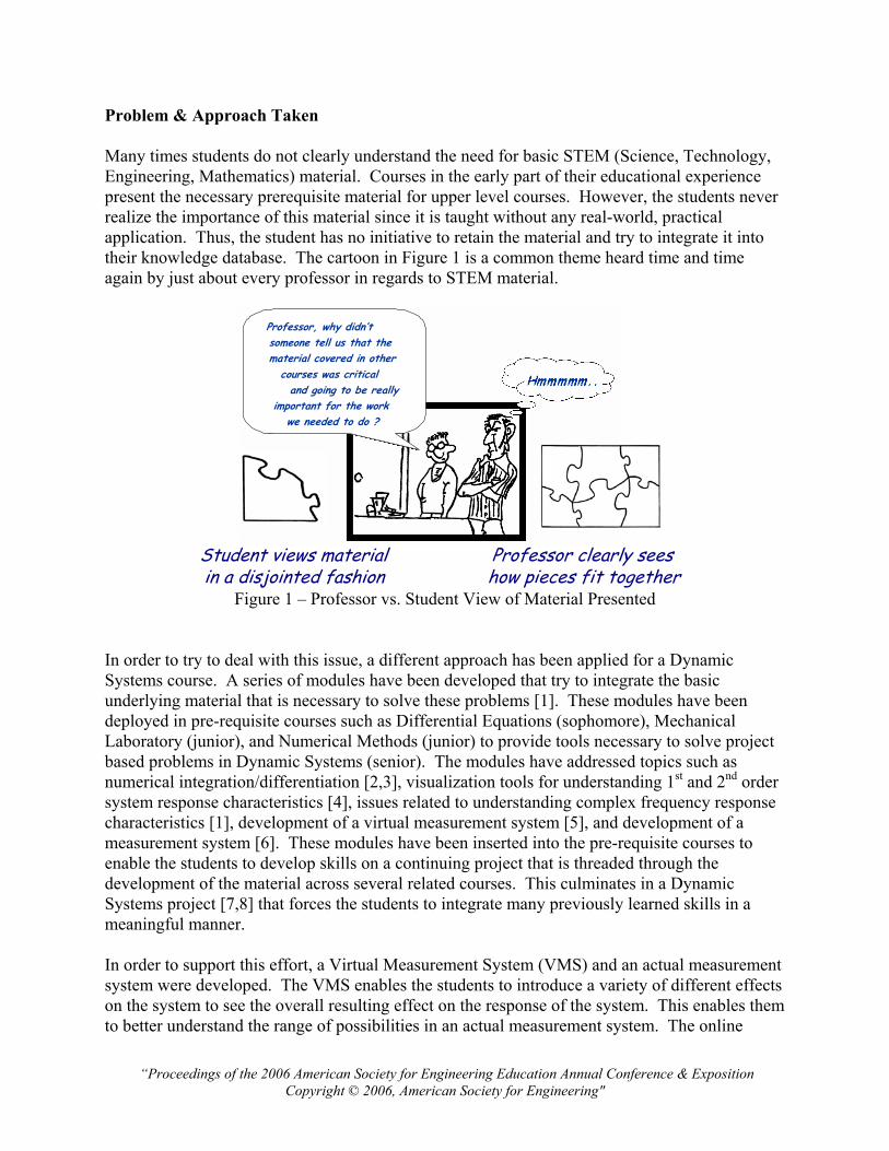
A variable spring is achieved with a variable length leaf spring supported with a coil spring. The variable spring stiffness allows the total spring stiffness to vary by approximately 20%. The leaf spring length is adjusted by a rack and pinion system that adjusts the support location for the leaf spring. A visual indication of the distance between the supports is identified by a scale. The leaf and spring coil arrangement is shown in Figure 18.

Figure 18: Leaf Spring/Coil Spring Arrangement

Dissipative forces are provided by an air dashpot with variable bleed orifice; the entire system is guided by a linear bearing system which is a very small portion of the entire dissipative force. These elements are shown in Figure 19.

Figure 19: Dissapative Elements

The input excitations are provided as a displacement via cam with variable length sprockets (different displacement inputs) or impulsive force via a solenoid device. These are shown in Figure 20.

Figure 20: Excitation Devices of the RUBE System


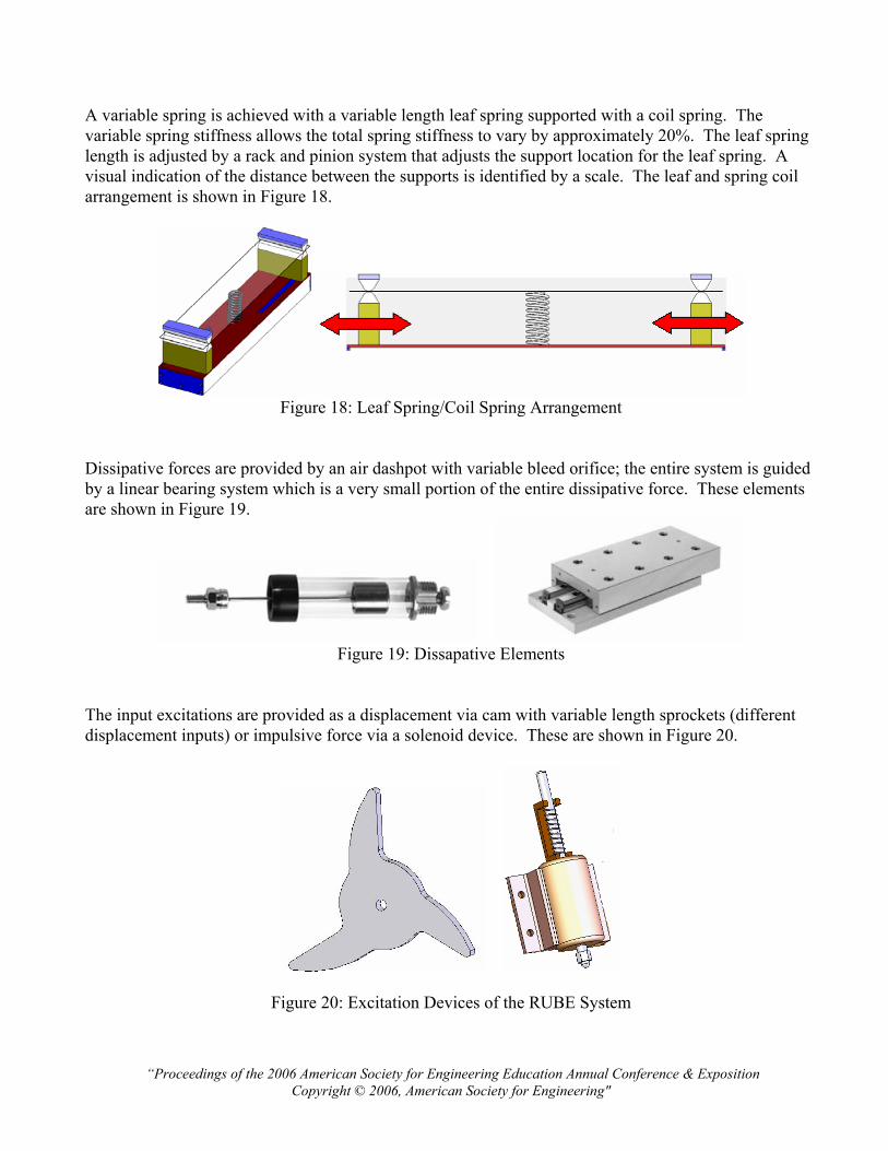
The RUBE online acquisition system graphical interface is shown in Figure 21. The LabVIEW [10] interface allows the user to gain control of the interface and run the experiment. If another user has control of the experiment, then a one minute time warning is given to allow the next user to gain control of the system. The user has the ability to look at any one, or all, of the transducers used for the measurement system. The interface provides flexibility to interrogate the measurement. The output data and video clip of the actual data run is saved to a separate web address that allows the user to access his/her data at any time. Some of these features are highlighted in Figure 22. In addition, a large set of previous runs that have been made are stored on the server so that users can also access previously collected data. This is needed especially when the internet traffic to the system is high and the user experiences a long wait due to numerous users waiting to access the system. A photograph of RUBE is shown in Figure 23.

Figure 21 – LabVIEW Interface of RUBE MCK System


Figure 22 – LabVIEW Interface of RUBE MCK System – Detailed Controls

Figure 23: RUBE Mechanical MCK System

The RUBE system feature is that every time the system is run, a different set of mass-damping-stiffness values exist. This allows students to each use the system and obtain unique characteristics that they must evaluate to determine the system characteristics – no two solutions are exactly alike. The variability on the system generally causes between 10% to 20% variation. This variation is shown in Figure 24 for identification of ranges that are typically experienced. In addition, three typical variations in response due to the individual variations in mass, damping and stiffness are shown.


m

k c

x=.14m

=.16k

HzfHz n 7.55.4 <<

m

k c

xm

k c

x=.14m

=.16k

HzfHz n 7.55.4 <<

0.5 1 1 .5 2 2.5 3

-0.6

-0.4

-0.2

0

0.2

0.4

No WaterAdded Water

0 0.5 1 1.5 2 2.5 3

-0.6

-0.4

-0.2

0

0.2

0.4

low dam pinghigh dam ping

0.5 1 1 .5 2 2.5 3

-0.6

-0.4

-0.2

0

0.2

0.412 Inch S upports16 Inch S upports

(Variation in response due to the design variables are in order of mass, damping, and stiffness, respectively)

(Specific values are not intended to be read in plots – only a conceptual overview of the range of values is intended)

Figure 24 – Schematic of RUBE Range of System Parameters and Effect on Response Student Reaction Various versions of the experimental system have been used for several years now. The latest version is the online RUBE system described herein. Student reaction to the system has been very positive. Several comments from surveys are presented. Student A - “With regards to previous course material (such as differential equations), it was very helpful to actually be forced to use earlier course material - I had to find my differential equations notebook and review some material before completing the first project. I feel that differential equations in particular is taught and then never used again, so that its significance is not clear until needed in this Dynamic Systems course.” “In terms of laboratory work requiring collection of data, this definitely helped me understand that these problems are not as simple as they might seem! In homework assignments, specific physical values are assigned to problems but when we actually have to find these values ourselves based on physical measurements of the system, and compare analytical models to measured results, we have a greater understanding of how imprecise this can be. For example, all of the calculations performed assume viscous damping, and in the mass-spring-dashpot system part of the damping is actually friction. We don’t have a clear understanding of the error that can be caused by this assumption until we actually see the results. We also become aware that there are multiple ways to determine the system characteristics of a physical system, and the importance of using multiple methods and comparing the results. Problems that seem easy when you do the homework at the end of a chapter in the text actually turn out


to be much more complicated in practice – you are forced to really think about the material and how it all fits together” Student B - "I almost always learn more completely when I do something as opposed to when someone instructs me. I believe relevant hands-on experience is much more effective than theory by itself. Struggling with a project makes me think harder and pursue other possible approaches to solving the problem. Project work forces me to learn the material to complete the assignment. This is not necessarily the case with homework problems taken from a book. When pressed for time, it is easy to copy the steps from examples and finish the assignment without understanding the problems. As a student, the ultimate goal is to learn the material so I can apply it once I graduate. These projects helped me understand the characteristics of a system and methods used to characterize dynamic systems. The group dynamics in project work are beneficial, as well. When members of our group disagreed, we were forced to dig deeper into what we were doing to find out who was right." Student C - “This class has taken an approach to material presentation that is unlike any previous class. The theory and materials are presented in the class periods, and are driven home during project preparation. The projects have forced the students to indeed “think outside the box”. This course curriculum has undoubtedly tied many ideas and previously learned material together. As a student that learns through hands on experience, as most students in this field are, I can say with conviction that due to the lab work associated with this class, I now understand the practical application of differential equations. As a part time student, it is common for there to be several semesters, sometimes years, separating Dynamic Systems from Differential Equations from Mechanical Engineering Laboratory. I have needed to spend time reviewing past material and I am now seeing this material in a new light. It is very fortunate that a class such as this is offered.” Student D - “Admittedly, the Dynamic System course required more work and time than many other courses I had taken before it. However, the hands-on approach and struggling through the projects is exactly the process by which the information was absorbed – by not only learning, but really understanding. Very few engineering courses are successful at integrating information from previous semesters into a logical path to a problem solution. Granted, many of the previously covered skills had to be reviewed, and possibly relearned in some instances. However, after having used these skills in solving more realistic engineering problems, hopefully relearning will not be needed in the future. The only other courses that have left me feeling as in control of the information learned were the Mechanical Engineering Laboratories, in which use of transducers and measurement equipment became second nature. Understandably, this is for the same reasons as the Dynamic Systems course. Logical assumptions, trial and error, and asking one’s self ‘does this make sense’ seem to be instinctive on the surface, however accepting that these are essential parts of engineering solutions and knowing how to use them wisely can only be developed in this type of realistic project setting. Likewise, working in groups of varying levels of understanding is required of professional engineers. One benefit of this course was that I learned that group members bring different qualities to the table. For example, while one member may not claim differential equations as a strong suit, that same member will notice the simplest, yet not the most obvious, method to determining the spring stiffness. In all, the time consumption and hard work paid off in not only learning the required information, but in understanding the engineering problem solving process much better.”


Student E – “As a recent transfer to the UMASS Lowell Mechanical Engineering program, my exposure to this type of hands on project was limited. Prior to this course, the important concepts of a particular subject did not necessarily “click” in the same semester in which I was taking the course. Many times I grasped the concepts in the following class which built upon the class I had just completed; this always left me feeling a semester behind. However, my experience in this Dynamic Systems course was different. In this course, the projects not only reinforced the material covered in lecture, but also went a few steps further by forcing us to think about which variables can affect the response of the systems we studied. These variables were not always intuitive and in order to obtain the correct response, they had to be addressed. The projects did not have simple solutions and involved interpretation of data, application of concepts discussed in lecture, and understanding of the physical system in the lab. Although I often struggled through each project, after obtaining the solution I had a much firmer understanding of the behavior of each of these systems.” Conclusion Student comprehension of basic STEM material for dynamic systems applications needs to be reinforced through active experiences. This is accomplished through a virtual measurement system which is a prelude to an actual experimental system. The Response Under Basic Excitation (RUBE) is a second order mechanical system which is available as an online experiment. An important feature of RUBE is that the system characteristics vary every time the system is accessed. The students are provided with supporting tutorial material, a virtual measurement system to explore numerous potential measurement difficulties and the actual measurement system. Overall the students have clearly indicated that the material presented has helped them to better understand the basic inherent material needed to solve the problems encountered in the measurement system. The measurement system has definitely helped the students to comprehend solutions to problems where clearly defined parameters are not available as is the case in most real-world situations. Acknowledgement Some of the work presented herein was partially funded by the NSF Engineering Education Division Grant EEC-0314875 entitled “Multi-Semester Interwoven Project for Teaching Basic Core STEM Material Critical for Solving Dynamic Systems Problems”. Any opinions, findings, and conclusions or recommendations expressed in this material are those of the authors and do not necessarily reflect the views of the National Science Foundation The authors are grateful for the support obtained from NSF to further engineering education. System Construction A complete set of drawings, bill of materials, Labview developed utilities are available upon request.


References 1. Avitabile,P., Pennell,S., White,J., “Developing a Multisemester Interwoven Dynamic Systems

Project to Foster Learning and Retention of STEM Material”, 2004 International Mechanical Engineering Congress and Exposition, Mechanical Engineering Education – Innovative Approaches to Teaching Fundamental Topics, ASME, Anaheim, CA, November 2004

2. Avitabile,P., Hodgkins,J., “Numerical Evaluation of Displacement and Acceleration for a Mass, Spring, Dashpot System”, 2004 ASEE Conference, Salt Lake, Utah, June 2004

3. Avitabile,P., McKelliget,J., Van Zandt,T., “Interweaving Numerical Processing Techniques in Multisemester Projects”, 2005 ASEE Conference, Portland Oregon, June 2005

4. Avitabile,P., Hodgkins,J., “Development of Visualization Tools for Response of 1st and 2nd Order Dynamic Systems”, 2006 ASEE Conference, Chicago, Illinois, June 2006

5. Avitabile,P., Van Zandt,T., “Developing a Virtual Model of a Second Order System to Simulation Real Laboratory Measurement Problems”, 2004 International Mechanical Engineering Congress and Exposition, Mechanical Engineering Education – Laboratory Instruction, ASME, Anaheim, CA, November 2004

6. Avitabile,P., Goodman,C., Van Zandt,T., “Development of a Measurement System for Response of a Second Order Dynamic System”, 2004 ASEE Conference, Salt Lake City, Utah, June 2004

7. Avitabile,P., et al., “Dynamic Systems Teaching Enhancement using a Laboratory-Based, Hands-On Project”, , 2004 ASEE Conference, Salt Lake City, Utah, June 2004

8. Avitabile,P., Hidgkins,J., Van Zandt,T., “Integrating Fundamental STEM Material in a Laboratory Based Dynamic Systems Course”, International Mechanical Engineering Congress and Exposition, Mechanical Engineering Education – Innovative Approaches to Teaching Fundamental Topics, ASME, Anaheim, CA, November 2004

9. The Dynamic Systems Website, http://dynsys.uml.edu/, with assorted tutorials, graphical user tools, and online data acquisition system http://dynsys.uml.edu/tutorials.htm http://dynsys.uml.edu/Acquisition_system/onlineacquisition.htm http://dynsys.uml.edu/downloads.htm

10. LabVIEW 7.1, National Instruments, Houston, Texas Peter Avitabile is an Associate Professor in the Mechanical Engineering Department and the Director of the Modal Analysis and Controls Laboratory at the University of Massachusetts Lowell. He has 30 years experience in design/analysis and modeling/testing dynamic/structural systems. He is a Registered Professional Engineer with a BS, MS and Doctorate in Mechanical Engineering. He is also a member of ASEE, ASME, IES and SEM. Tracy Van Zandt, Nels Wirkkala and Jeff Hodgkins are Graduate Students in the Mechanical Engineering Department at the University of Massachusetts. They are currently working for their Master’s Degrees in the Modal Analysis and Controls Laboratory while concurrently working on an NSF Engineering Education Grant directed towards integrating STEM material critical for understanding dynamic systems response.


Appendix – Detailed Information Regarding the RUBE System This online experiment allows the user to collect data on the motion of a second-order mass-spring-dashpot system. The properties of the system vary with time—the moving mass of the system includes a small water tank which fills and gradually drains, and the spring portion of the system includes a leaf spring which changes in length each time the system is activated. In addition, three different initial displacements are available as inputs to the system. Consequently, each user of the system will obtain slightly different results. Multiple different transducers are used to collect acceleration and displacement data for the motion of the system. Good transducers are available, which provide relatively clean data. However, “bad” transducers—contaminated by noise, drift, or bias—are also used. Mass Related Components The moving mass of the system consists of the sum of the mass of the water and the mass of all of the other moving parts of the system. This is shown schematically in Figure A1. The masses of some system components are given in Table A1. The water tank has an inner diameter of 2.4 inches, and a maximum possible water height of 4 inches. The height of the water in the tank for each run can be determined from the video/photograph of the system. Though the level of water in the tank is changing continuously, the mass of water in the tank only changes at an average rate of 0.1% during one system run.

Figure A1: Variable Mass

Component Weight (Ounces) Water Reservoir (with valve) 1.73 Inlet hose 0.54 Outlet hose (including water) 0.18 Linear bearing 28.80 Brackets, nuts, washers, etc. 13.56

Table A1: Some Weights Associated with the Mass Component of the System


Stiffness Related Components The stiffness related components consist of a coil spring and a leaf spring as shown in Figure A2. The coil spring is fixed in dimension but the leaf spring has a variable length (between 9 to 14 inches) and is changed every time the system acquisition system is initiated. The properties of the coil spring and leaf spring are shown in Tables A2 and A3, respectively.

Figure A2: Schematic Showing Leaf Spring/Coil Spring Arrangement

Property Value

Spring material Round steel music wire, ends closed and ground

Overall Length 2.46 in

Outside Diameter (OD) 0.54 in

Wire Diameter (d) 0.049 in

Number of Coils 4.32

Table A2: Properties Associated with the Coil Spring

Property Value Material Aluminum Modulus of elasticity 1.00E+07 psi Yield strength 50000 psi Fatigue Strength (500,000,000 cycles) 20000 psi Length 9 in to 14 in Thickness 0.032 in Width 4 in

Table A3: Properties Associated with the Leaf Spring Effective stiffness characteristics can be determined from a Dynamic Systems textbook from material on mechanical systems or from any Design of Machine Elements textbook or other Mechanical Engineering related handbook.


In addition to analytical methods for determining these stiffnesses, a set of data on the leaf spring was collected for various effective lengths and is shown in Table A4 below and plotted in Figure A3.

Leaf Spring

Span --> Deflection Force Deflection Force Deflection Force

0 0 0 0 0 01 0.07 0.35 0.104 0.42 0.108 0.342 0.142 0.73 0.198 0.8 0.21 0.663 0.219 1.11 0.272 1.08 0.302 0.964 0.277 1.43 0.355 1.42 0.407 1.285 0.345 1.76 0.431 1.7 0.503 1.586 0.42 2.14 0.502 1.97 0.599 1.867 0.478 2.43 0.7 2.168 0.538 2.72 0.804 2.469 0.902 2.7210 1 2.98

L = 10 inches L = 11 inches L = 12 inches

Leaf Spring Span -->

Deflection Force Deflection Force Deflection Force Deflection Force0 0 0 0 0 0 0 0

1 0.104 0.26 0.121 0.24 0.116 0.18 0.051 0.062 0.202 0.5 0.203 0.4 0.206 0.34 0.1 0.123 0.304 0.76 0.302 0.62 0.309 0.5 0.199 0.244 0.405 1 0.404 0.82 0.4 0.64 0.297 0.385 0.496 1.22 0.506 1.02 0.504 0.8 0.404 0.56 0.604 1.48 0.606 1.2 0.606 0.96 0.507 0.647 0.702 1.68 0.7 1.38 0.707 1.1 0.604 0.768 0.807 1.92 0.806 1.56 0.802 1.24 0.701 0.829 0.904 2.11 0.898 1.74 0.904 1.4 0.805 0.9810 1 2.31 1 1.9 1 1.54 0.905 1.08

L = 13 inches L = 14 inches L = 15 inches L = 16.4 inches

Table A4: Leaf Spring Stiffness Measurements

Spring Test

y = 2.2932x + 0.0563R2 = 0.9985

y = 5.0674x + 0.0072R2 = 0.9998

y = 3.8945x + 0.0231R2 = 0.9998

y = 2.9709x + 0.0556R2 = 0.9991

y = 1.896x + 0.0365R2 = 0.9987

y = 1.5246x + 0.0232R2 = 0.9996

y = 1.1858x + 0.0138R2 = 0.9977

0

0.5

1

1.5

2

2.5

3

3.5

0 0.2 0.4 0.6 0.8 1 1.2

Deflection (IN)

Forc

e (L

BF)

L = 10 inchesL = 11 inchesL = 12 inchesL = 13 inchesL = 14 inchesL = 15 inchesL = 16.4 inches

Figure A3: Force Deflection Data for Leaf Spring


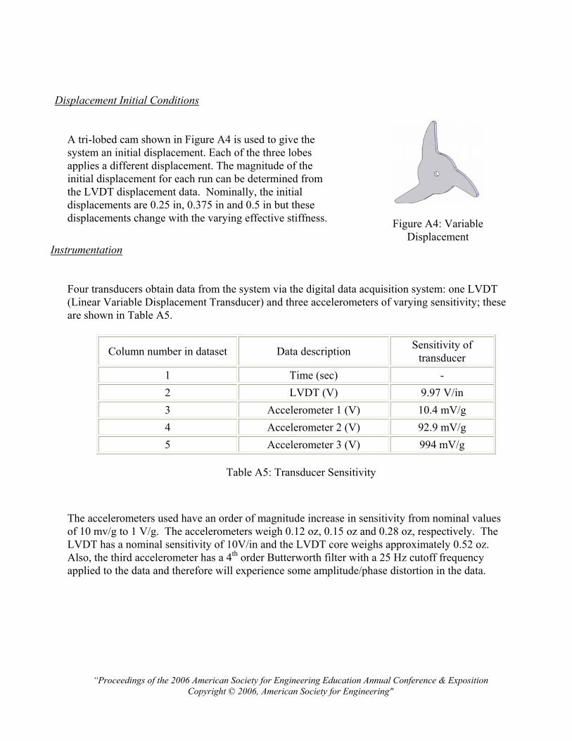
Displacement Initial Conditions

A tri-lobed cam shown in Figure A4 is used to give the system an initial displacement. Each of the three lobes applies a different displacement. The magnitude of the initial displacement for each run can be determined from the LVDT displacement data. Nominally, the initial displacements are 0.25 in, 0.375 in and 0.5 in but these displacements change with the varying effective stiffness.

Figure A4: Variable Displacement

Instrumentation

Four transducers obtain data from the system via the digital data acquisition system: one LVDT (Linear Variable Displacement Transducer) and three accelerometers of varying sensitivity; these are shown in Table A5.

Column number in dataset Data description Sensitivity of transducer

1 Time (sec) - 2 LVDT (V) 9.97 V/in 3 Accelerometer 1 (V) 10.4 mV/g 4 Accelerometer 2 (V) 92.9 mV/g 5 Accelerometer 3 (V) 994 mV/g

Table A5: Transducer Sensitivity

The accelerometers used have an order of magnitude increase in sensitivity from nominal values of 10 mv/g to 1 V/g. The accelerometers weigh 0.12 oz, 0.15 oz and 0.28 oz, respectively. The LVDT has a nominal sensitivity of 10V/in and the LVDT core weighs approximately 0.52 oz. Also, the third accelerometer has a 4th order Butterworth filter with a 25 Hz cutoff frequency applied to the data and therefore will experience some amplitude/phase distortion in the data.


Typical Data File Layout A typical excerpt of the text file containing the data acquired is shown below for reference.

LabVIEW Measurement Writer_Version 0.92 Reader_Version 1 Separator Tab Multi_Headings Yes X_Columns One Time_Pref Absolute Operator Administrator Date 2005/07/27 Time 14:56:34.531125 ***End_of_Header*** Channels 4 Samples 4000 4000 4000 4000 Date 2005/07/27 2005/07/27 2005/07/27 2005/07/27 Time 14:56:42.528999 14:56:42.528999 14:56:42.528999 14:56:42.528999 Y_Unit_Label Volts Volts Volts Volts X_Dimension Time Time Time Time X0 0.0000000000000000E+0 0.0000000000000000E+0 0.0000000000000000E+0 Delta_X 0.002000 0.002000 0.002000 0.002000 ***End_of_Header*** X_Value LVDT Accel 1 Accel 2 Accel 3 Comment 0.000000 -1.672363 0.002441 0.000000 0.002441 0.002000 -1.667480 0.002441 0.000000 0.002441 0.004000 -1.672363 0.002441 0.000000 0.002441 0.006000 -1.669922 0.000000 0.000000 0.002441

7.980000 -5.000000 0.000000 0.034180 0.168457 7.982000 -5.000000 -0.002441 0.039062 0.178223 7.984000 -5.000000 -0.004883 0.070801 0.185547 7.986000 -5.000000 -0.007324 0.095215 0.195312 7.988000 -5.000000 -0.004883 0.095215 0.209961 7.990000 -5.000000 -0.012207 0.087891 0.236816 7.992000 -5.000000 -0.007324 0.041504 0.275879 7.994000 -5.000000 -0.007324 0.024414 0.334473 7.996000 -5.000000 -0.004883 0.112305 0.405273 7.998000 -5.000000 -0.004883 0.083008 0.483398

Documents

SECOND ORDER MECHANICAL ONLINE …faculty.uml.edu/pavitabile/dynsys.uml.edu/papers/ASEE_2006/ASEE... · [email protected] ... “Proceedings of the 2006 American Society for