SECOND ORDER MEASUREMENT SYSTEMSmyweb.astate.edu/sharan/PMC/Labs/ME3504 2nd... · Second Order Systems - 2 THE MASS/SPRING/DAMPER SYSTEM A model for the single degree of freedom mass/spring/damper

Second Order Systems - 1

SECOND ORDER MEASUREMENT SYSTEMS Earlier in this course we considered first order measurements systems such as the thermocouple. A transducer was defined as a first order system if there was one dominating energy store. In the case of the thermocouple, this energy store was the heat capacity of the thermocouple’s bead or crimp. We now turn to second order transducers. A transducer is defined as a second order system if it has two predominant energy stores. Consider, as an example, a spring balance. The spring can obviously store strain energy. Additionally the mass of the system (the mechanism as well as the mass we are measuring) can store energy – kinetic energy. When taking dynamic measurements (i.e. measuring something that is changing with time), the energy in the system transfers back and forth between the two forms. In the spring balance example, strain energy transforms to kinetic energy, which transforms back to strain energy, and so on. In this section of the course, we investigate the effect this has on a transducer’s performance. We start by looking at the basic equations of motion for a 2nd order system. Since most mechanical engineering second order transducers are built on mass/spring/damper concepts, we develop the theory for this type of system. We then apply it to a force gage, the seismograph and the accelerometer. Other types of systems can be analyzed by a suitable substitution of symbols. A note: This handout does not develop the details of the theory. The handout is primarily intended to present the background to 2nd order systems, and then give information that can be used for the interpretation of measurement systems. For those interested in the theoretical basis, there are many standard textbooks available that give a rigorous mathematical development.


THE MASS/SPRING/DAMPER SYSTEM A model for the single degree of freedom mass/spring/damper system is shown below, along with a free body force diagram. In this model, the mass is m, the spring stiffness is k, and the viscous damping coefficient is c. Time-varying force f is applied to the mass, and the displacement response of the mass is x.

kc

mx

f

kx c dx/dt

f Without damping, the energy stored in the spring and mass would never dissipate, and the system would never “settle”. In this course we will use viscous damping as the energy dissipation mechanism. Viscous damping generates an opposing force that is proportional to velocity:

DAMPING

dxF c

dt=

where c is the viscous damping constant with units of force per unit speed. This type of damping is often considered for this type of second order system because it is reasonably representative of the energy dissipation methods in many engineering structures. It is also mathematically the easiest form of damping to apply to transient vibrations. Noting that the spring generates a force proportional to its displacement, Newton’s Second Law (F = ∑ma) is applied to the FBD get:

− − =2

2

dx d xf kx c m

dt dt

We now introduce three new symbols.

Static sensitivity,1

SKk

= (note that KS and k are different!)

Circular natural frequency, ω =n

km

Viscous damping ratio, ζω

= =2 2n

c cm km


The static sensitivity, KS, should really be called the pseudo-static sensitivity. It is determined as the response of the measurement system if it had no mass and no damping – i.e., the response of the equivalent zero-th order system. Note that KS has units that depend on the properties being measured. The circular natural frequency, ωn, is the frequency the device would vibrate at in the absence of damping. It has units of radians per second. The equivalent natural frequency, fn, has units of Hertz. The two frequencies are related by ω π= 2n nf . CAUTION: Make sure you are using the correct units in your calculations. The viscous damping ratio is a nondimensional measure of energy dissipation. A system with very low damping will continue to vibrate for a long time after input is stopped or changed. Low damping may also cause very large motion if sinusoidal excitation is close to the natural frequency. Conversely, a system with very large damping will not have excessive vibration at resonance, but it will take a long time to respond to changes in input.

If ζ < 1.00 the system is called under-damped.

If ζ > 1.00 the system is called over-damped.

The critical damping value is when 1.00ζ = . It defines a ‘change-over’ in our analysis strategy. When ζ < 1.00 we need different equations than if ζ > 1.00 . It is most unlikely that you will come across a real measurement system where the viscous damping ratio is exactly ζ = 1.00 .

Incorporating these new symbols into the equation of motion and rearranging yields the following equation, which is the basic starting point for much of the later work in this handout:

22

22 n n

d x dx fx

dt mdtζω ω+ + =

This is a ‘clumsy’ way of writing out the equation, and we will use the standard “dot” notation for differentiation with respect to time. That is:

2

2 and

dx d xx x

dt dt= =& &&

The equations now become: 22 n n

fx x x

mζω ω+ + =&& &

Read this equation as “x-doubledot plus 2 zeta omega sub n x-dot plus omega sub n squared x = f/m”.


THE FORCE GAUGE A force gauge measures force! Typical force gauges can be high-stiffness piezo-electric devices as well as relatively low stiffness devices such as the spring balance. Slight modification to the concept means that a force gauge can also measure pressure. The pressure is applied to the surface area of the mass, causing a force. Thus the analysis of the pressure transducer is essentially the same as the analysis of a force gauge. Note that in this course we do not investigate the effect of sensing lines that are often found on pressure measuring systems. There are two types of excitation input that we wish to consider. These are a step input, and sinusoidal input. The step input is representative of what happens when, for example, a weight is suddenly applied to a spring balance. The response to sinusoidal input is the essential building block to the analysis of many periodic signals, where we use spectral analysis to break down a periodic signal into a combination of sinusoidal inputs. When we use a 2nd order system to measure force, the input to the transducer is the force. The ‘raw’ output of the transducer is the absolute displacement of the mass. However, this parameter is of little use – we are using the transducer to measure the actual force – we don’t want to know the displacement of the transducer. We therefore use the symbol yF to define the output of our transducer after it has been converted to force. The transducer output yF will be in units of pounds or Newtons. The conversion uses the static sensitivity, KS, or the spring stiffness, k, such that:

FS

xy kx

K= =

In a real measurement system, the ‘raw’ output from a force transducer is usually not displacement, x. It is usually electrical charge, strain, displacement, or whatever. This quantity is converted in the signal conditioning part of the measurement system, where it is most often converted to Volts. A data logger, display or other method then converts the Volts into engineering units of force. The above equation is the mathematical representation of the entire procedure of converting the displacement of the mass in the force gauge into a force measurement.

FORCE TRANSDUCER

SIGNALCONDITIONING

RAW SIGNAL

VOLTS

FORCE


The modified equation of motion for the transducer is: 2

22

2

2

2

SF Fn n F

SF n F n F

K fd y dyy

dt mdtK f

y y ym

ζω ω

ζω ω

+ + =

+ + =&& &

REMEMBER: f is the force we are trying to measure. It varies with time.

yF is the time varying force output from the transducer, i.e. what the transducer is showing us as the measurement of force. If the transducer were ‘exact’, yF and f would be the same. But because f is varying with time, some error is introduced into yF.

FORCE GAUGE RESPONSE TO STEP INPUT A step force input is defined by:

< => =

0 00

t ft f F

The output response of the transducer (in pounds or Newtons) depends on the viscous damping ratio, as follows:

( ) ( )

( ) ( )

2

2

2

2

1 2

2

sinh 11 : 1 cosh 1

1

sin 11 : 1 with sin 1

1

n

n

ntF

n

n

ntF

tye t

F t

tye

F

ζω

ζω

ζ ω ζζ ω ζ

ω ζ

ω ζ φζ φ ζ

ζ

−

− −

− > = − − + −

− − < = − = −

−

Some examples of these curves are shown in the following figure. Note that the long-term equilibrium response is yF / F = 1. Thus, after a sufficiently long time has elapsed, the output from the transducer tends to the correct value of the applied force. Also note that the transducer output reaches the correct value most quickly, and with minimum

overshoot if the damping ratio is given by ζ = =1

0.7072

.


0 5 10 15 20

0.5

1

1.5

2

z=0.05z=0.2z=0.707z=1.0z=2.0

Nondimensional time (omega t)

y_F/

F

Note that this is a “MathCAD plot”. The annotation y_F/F means FyF

and the notation

z=0.05, etc., means ζ=0.05 etc. We will see this type of plot and notation several times more in this handout. Typical accuracy problem. A typical question would be, “How long do we have to wait after the step input is applied before the transducer output is within a certain accuracy?” Let us assume that we want to guarantee that the transducer output is within 2% of the actual force value. We first decide whether ζ < 1.00 or ζ > 1.00 . When ζ > 1.0 we solve the response equation to determine the time when the output is at 98% of the input, i.e., solve the following for t:

( ) ( )ζω

ζ ω ζω ζ

ω ζ−

− = = − − + −

2

2

2

sinh 10.98 1 cosh 1

1n

ntF

n

n

tye t

F t

When ζ < 1.0 we need to consider the envelope of the decaying sine-wave response. The envelope is the curve that touches the bottom (or top) peaks of the response trace. Mathematically, this is achieved by replacing the sine function with its maximum and


minimum values of +/-1. The following figure gives one example of the step response for ζ = 0.10. The two envelopes are shown as dashed lines. The envelopes on the figure have the equations:

ζω ζω

ζ ζ

− −

= − = +− −2 2

1 (lower envelope); 1 (upper envelope)1 1

n nt tF Fy ye e

F F

We can determine the time when the output is guaranteed to be within (e.g.) 2% of the correct value by solving one of the following for t. Note that this method does not give you the exact time when the signal is within the required accuracy. However, the method is sufficiently accurate for most instrumentation needs. If you are designing a measurement system and need more accuracy than this method can give, you are either working on a very specialist instrumentation problem, or you probably have a poor design for your system!

ζω ζω

ζ ζ

− −

= = − = = +− −2 2

0.98 1 (lower envelope); 1.02 1 (upper envelope)1 1

n nt tF Fy ye e

F F

0 10 20 30 40

0.5

1

1.5

2

Nondimensional (omega t)

y_F/

F


FORCE GAUGE RESPONSE TO SINUSOIDAL INPUT We start with the same basic equation of motion.

22F n F n F

Kfy y y

mζω ω+ + =&& &

The full solution of this equation includes both the general solution and the particular solution. The general solution represents the response of our system during the initial period soon after the excitation has been applied. This is the transient solution, and is similar to the response caused by a step input (previous section of this handout). Often when measuring a time-varying force we are using the transducer to measure signals that have been going on for a long period of time. For example, we may be measuring the noise generated by an internal combustion engine, or we may be monitoring the vibration of a gas turbine. In most of these cases the transient effect dies away comparably quickly, and we are only interested in the particular solution. Therefore, this handout only considers the particular solution, which is also called the steady state response or (in some books) the equilibrium response. For sinusoidal input the force excitation on the transducer is given by:

( )ω= cosf F t F is the amplitude of the exciting force, and ω is the frequency of the force in radians per second. The displacement response of the mass in the force gauge, x, is given by:

( ) ζωωω φ φ

ω ω−

= − = − 1

2 2

2sin with tan n

n

x X t

But, as before, we are not really interested in the displacement of the mass in our force gauge. We need to convert this to something useful – i.e., a force. Again, we convert the displacement motion of the transducer’s mass into a force output using the static sensitivity:

FS

xy kx

K= =

The steady state response of the transducer is now given by:

( ) ( )sin sinF Fs

Xy t Y t

Kω φ ω φ= − = −


REMEMBER: F is the amplitude of the sinusoidal force excitation. It is a constant.

yF is the time varying force output from the transducer, i.e. what the transducer is showing us as the measurement of force.

YF is the amplitude of the force output from the transducer. If the transducer

were ‘exact’, YF and F would be the same. But because f is varying with time, some error is introduced into both yF and YF.

ω The frequency (in radians per second) of the excitation φ Is the phase lag (radians) of the transducer output compared to the actual

exciting force. If the transducer were ‘exact’, φ would be the zero. But because f is varying with time, φ is not zero.

KS is the static sensitivity = 1 / k Let’s look at how the amplitude and phase of the output from our force gauge depend on the frequency of the input. As before, in this handout we do not go into the details of the theoretical development. Rather, we present the results in a format suitable for the analysis of measurement systems. The amplitude of the force output of our transducer is given by:

ω ωζ

ω ω

= − +

22 2

2

1

1 4

F

n n

YF

and the phase is

ωζ

ωφ

ωω

−

= −

12

2tan

1

n

n

Note that the output of our force gauge depends on both the amplitude of the exciting force, as well as the frequency of the exciting force. Let us look at how the transducer output varies with the frequency of the force.


0 0.5 1 1.5 2 2.5 30

2

4

6

8

10

12

z=0.05z=0.2z=0.707z=1.0z=2.0

Nondimensional frequency (omega/omega_n)

Y_F

/F

Again, this is a “MathCAD format” plot, so z=ζ. We make the following observations:

When the excitation frequency is close to the natural frequency (i.e., ω ≈ ωn) the transducer gives a large output when damping is ‘light’ – i.e. if ζ is small. This suggests that we do not want to use a force gauge at frequencies close to its natural frequency. When the excitation frequency is very high (i.e. ω is much greater than ωn ) the output of the transducer is always much lower than the force we are measuring. This suggests that we do not want to use a force gauge at frequencies above its natural frequency. If we look at the lowest frequencies we see that for a short frequency range, the output of the transducer is the same as the amplitude of the excitation, YF / F = 1. Let’s look at this on a logarithmic frequency scale.


0.01 0.1 1 100

2

4

6

8

10

12

z=0.05z=0.2z=0.707z=1.0z=2.0


Y_F

/F

Looking at this graph we can see that providing the excitation frequency is well below the natural frequency, the amplitude of the force gauge’s output is very close to the actual force amplitude. What about the phase? The following figure shows the phase of the transducer output compared to the original force signal.


0.01 0.1 1 100

45

90

135

180

z=0.05z=0.2z=0.707z=1.0z=2.0


Phas

e (d

egre

es)

For an “accurate” force gauge, we want the phase of the transducer output to be zero compared to the original signal. The indication from the phase figure above is that there can be large errors in phase, especially if the damping is high or the frequency of the signal is anywhere near the natural frequency of the force gauge.

FORCE GAUGE

When measuring sinusoidal force signals with a force gauge, we need to ensure that the natural frequency of the force gauge is well above the frequency of the signal we

are measuring.

How do we calculate the useful frequency range? We have to decide on both the phase and amplitude limits, and take the one that is most stringent. Typical homework or test problems will probably only ask for either the phase or amplitude limit, but be prepared to deal with the full problem.


Deciding On The Useful Frequency Range Of A Force Gauge Based On Phase Restrictions. The procedure is relatively simple. Determine the natural frequency of the transducer and decide on an acceptable phase error. WATCH UNITS. Then solve the following equation for the excitation frequency, ω. Note that the phase depends on the ratio of excitation frequency to natural frequency, / nω ω . Thus, depending on how the question is worded, you may not need to know the actual natural frequency for all problems.

( )

ωζ

ωφ

ωω

=

−

2

2tan

1

n

n

Deciding On The Useful Frequency Range Of A Force Gauge Based On Amplitude Restrictions. This exposition only details the cases when ζ < about 0.6 and ζ >1.0. This is because when the damping ratio is in the approximate range of 0.6 < ζ < 1.0, the “resonant peak” is very small or non-existent. We do not immediately know, therefore, whether we should use a factor of (1+error) or (1-error) in the calculations. When the damping ratio is in this ‘middle’ range, we need to calculate the useful range using both (1+error) and (1-error) factors, and then determine the range by interpreting those numbers and the graphs. When ζ > 1.0 the amplitude output of our force gauge is always less than the original signal, irrespective of excitation frequency. For (e.g.) a 2% error we solve the following equation for the excitation frequency, ω.

22 2

2

11 0.02 0.98

1 4

F

n n

YF

ω ωζ

ω ω

= − = = − +

We will obtain one positive solution for ω2, which gives the answer we are seeking.


When ζ < 0.6 (approximate number) the amplitude output of our force gauge in the region of resonance is greater than the original signal. For (e.g.) a 2% error we solve the following equation for the frequency ratio / nω ω and hence the excitation frequency, ω.

22 2

2

11 0.02 1.02

1 4

F

n n

YF

ω ωζ

ω ω

= + = = − +

We will obtain two positive solutions for ω2. Looking at the figure we see that the lower value defines the frequency range we are interested in. The higher value gives the frequency above resonance that also has 2% error. However, the slope of the curve is very large. Small variations in the natural frequency of our transducer (e.g. by slightly different mounting procedures) will make the exact value of this higher frequency vary a lot. Therefore, we discard the higher result and conclude that we cannot use the transducer at this frequency. Example. A force transducer is mounted such that its total effective weight is 0.75 lbs. When a static force of 1,000 lb is applied to the transducer, it deflects by 0.015 ins. Damping in the transducer system is estimated as ζ = 0.15. Calculate the useful frequency range for a maximum amplitude error of 5%. Also calculate the phase error at this frequency limit. First we calculate the effective stiffness.

( )δ= = = × 31000

800 10 lb/ft0.015/12

Wk

And then the natural frequency.

( )ω = = = =

800,0005860 rad/s 933 Hz

0.75 / 32.2n

km

We note that ζ is less than 0.6, so we solve the following:

ω ωω ωζ

ω ω

ω

= = = − + × × − +

= × ×

2 22 2 2 222

2 6 3

1 11.05

1 4 0.151 45860 5860

63.872 10 or 1.716 10

F

n n

YF

This gives us two frequencies:

ω ω= = = =7990 rad/s 1272 Hz and 1310 rad/s 208.5 Hz


The useful frequency range is defined by the lower solution as:

zero < useful range < 208.5 Hz Finally we calculate the phase lag at 1310 rad/s:

ωζ

ωφ

ωω

− −

× × = = = −−

1 12 2

13102 2 0.155860tan tan 4.04

131011

5860

On

n

THE 2nd ORDER SEISMIC TRANSDUCER One problem engineers frequently come across is measuring the time-varying motion of something when there is no absolute fixed reference to use as a guide. For example, we may want to measure the displacement of the earth when there is an earthquake, or the acceleration of a diesel engine at sea. To make this type of measurement we use a seismic device such as a vibrometer, seismograph or accelerometer. These are second order systems where we relate the change in length of the spring element to the motion of the ‘ground’. We define the following symbols:

s Time-varying absolute motion of the ground (this is what we are trying to measure)

x Time-varying absolute motion of the mass in the transducer Schematic and free body force diagrams for the seismic measurement system are as follows:

m

k c

x

s

k(s-x)

c (ds/dt-dx/dt)


Applying Newton’s Second Law (F = ∑ma) we obtain:

( ) ( )− + − =& & &&k s x c s x mx This shows that the force on the mass depends on the relative displacement (and relative velocity) of the two ends of the spring/damper units. We define the following symbol:

yS The time-varying relative motion of the mass with respect to the ground, yS = (s-x). This is also the time-varying output of the transducer.

The equation of motion now becomes:

+ + = &&&& &S S Smy cy ky ms

Note that this equation relates the relative motion of the transducer, yS, to the absolute motion of the ground. Something like this is an essential requirement for a seismic device. SEISMIC DISPLACEMENT TRANSDUCER RESPONSE TO STEP INPUT Seismic second order displacement transducers such as vibrometers and seismographs, whose output is proportional to the relative displacement of the spring/damper element, are unsuitable for the measurement of a step displacement input. There are several reasons for this. The easiest reason to understand (without getting involved in a detailed mathematical analysis) is that after the ground has moved through its step input, the mass will vibrate. After the transient effect has decayed away, the mass will come back into static equilibrium. The only way it can do this is if the spring force is equal to the weight of the mass, which was also the condition before the step occurred. Thus, the final output of the transducer is yS = (s-x) = zero. Hardly the result we want! If it is necessary to measure a step type of displacement input, a different type of displacement transducer must be used. There are several different kinds of displacement transducers that are suited for this situation, but their description and analysis are beyond the scope of this unit on 2nd order systems.


SEISMIC DISPLACEMENT TRANSDUCER RESPONSE TO SINUSOIDAL INPUT We define the following symbols:

s Time-varying absolute motion of the ground S Amplitude of s. Recall that we are trying to measure s and S yS The time-varying relative motion of the mass with respect to the ground,

yS = (s-x). This is also the time-varying output of the transducer. YS Amplitude of yS ω The frequency (in radians per second) of the excitation φ The phase lag (radians) of the transducer output compared to the

ground’s displacement. If the transducer were ‘exact’, φ would be the zero. But because s is varying with time, φ is not zero.

For sinusoidal displacement input from the ‘ground’ we have:

( ) ( )ω ω φ= = −sin sinS Ss S t y Y t As before, we do not go into the detailed theoretical development. Rather, we just present the results. First, the amplitude response is given by:

ωω

ω ωζ

ω ω

=

− +

2

1/ 222 2

21 4

nS

n n

YS

and the phase is

( )

ωζ

ωφ

ωω

=

−

2

2tan

1

n

n


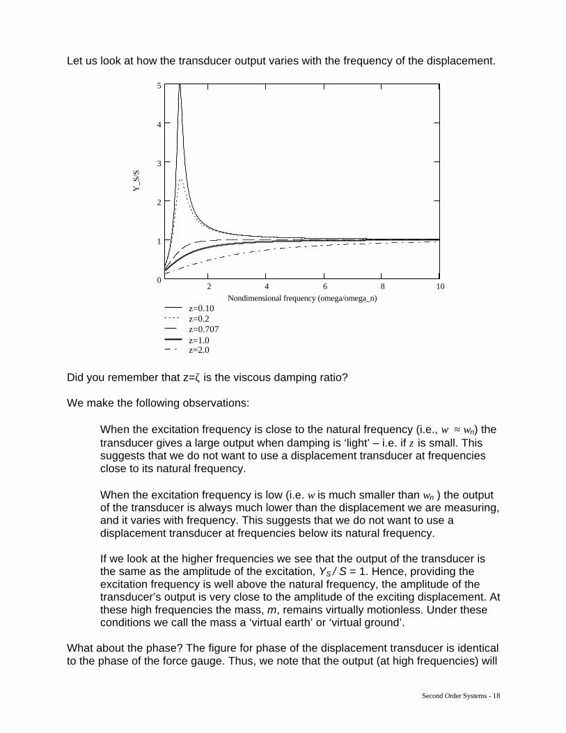
Let us look at how the transducer output varies with the frequency of the displacement.

2 4 6 8 100

1

2

3

4

5

z=0.10z=0.2z=0.707z=1.0z=2.0


Y_S

/S

Did you remember that z=ζ is the viscous damping ratio? We make the following observations:

When the excitation frequency is close to the natural frequency (i.e., ω ≈ ωn) the transducer gives a large output when damping is ‘light’ – i.e. if ζ is small. This suggests that we do not want to use a displacement transducer at frequencies close to its natural frequency. When the excitation frequency is low (i.e. ω is much smaller than ωn ) the output of the transducer is always much lower than the displacement we are measuring, and it varies with frequency. This suggests that we do not want to use a displacement transducer at frequencies below its natural frequency. If we look at the higher frequencies we see that the output of the transducer is the same as the amplitude of the excitation, YS / S = 1. Hence, providing the excitation frequency is well above the natural frequency, the amplitude of the transducer’s output is very close to the amplitude of the exciting displacement. At these high frequencies the mass, m, remains virtually motionless. Under these conditions we call the mass a ‘virtual earth’ or ‘virtual ground’.

What about the phase? The figure for phase of the displacement transducer is identical to the phase of the force gauge. Thus, we note that the output (at high frequencies) will


be 180O out of phase with the input. We can easily deal with a phase of 180O since it is essentially ‘just’ a +/- sign error that we can correct for.

SEISMIC DISPLACEMENT TRANSDUCER

When measuring displacement with a 2nd order seismic displacement transducer, we

need to ensure that the natural frequency of the transducer is well below the frequency of the signal we are measuring.

COMPARISON BETWEEN A FORCE GAUGE AND A SEISMIC DISPLACEMENT TRANSDUCER Both transducers are second order systems. Hence they follow the same basic equations of motion. The detailed equations (given above in this handout) are slightly different, since we need to calculate slightly different things. Normally, we would not use either transducer to measure signals when the excitation frequency is close to the natural frequency of the transducer. That is, nω ω≈ . The second order system can be used as a force gauge when the excitation frequency is much lower than the natural frequency. That is nω ω<< . The device can be used to measure a step change. The second order system can be used as a displacement transducer when the excitation frequency is much higher than the natural frequency. That is nω ω>> . The device cannot be used to measure a step change.


Deciding On The Useful Frequency Range Of A Displacement Transducer Based On Amplitude Restrictions. This exposition only details the two cases (ζ < about 0.6 and ζ >1.0). This is because when the damping ratio is in the approximate range of 0.6 < ζ < 1.0, the “resonant peak” is very small or non-existent. We do not immediately know, therefore, whether we should use a factor of (1+error) or (1-error) in the calculations. Therefore we need to calculate the answer for both factors, and then interpret the result using the graph to decide on the useful range. When ζ > 1.0 the amplitude output of our displacement transducer is always less than the original signal. For (e.g.) a 2% error we solve the following equation for the excitation frequency, ω.

2

1/ 222 2

2

1 0.02 0.98

1 4

nS

n n

YS

ωω

ω ωζ

ω ω

= − = =

− +

We will obtain one positive solution for ω2, which gives the answer we are seeking. When ζ < 0.6 (approximate range) the amplitude output of our displacement transducer in the region of resonance is greater than the original signal. For (e.g.) a 2% error we solve the following equation for the excitation frequency, ω.

2

1/ 222 2

2

1 0.02 1.02

1 4

nS

n n

YS

ωω

ω ωζ

ω ω

= + = =

− +

We will obtain two positive solutions for ω2. Looking at the graph we see that the higher value defines the frequency range we are interested in. Comparable to the analysis for a force gauge, we see that the lower value gives the frequency below resonance that also has 2% error. However, the slope of the curve is very large. Small variations in the natural frequency of our transducer (e.g. by slightly different mounting procedures) will make this lower frequency change a lot. Therefore, we discard the lower result. Also, remember that we cannot use this device to measure displacement when the excitation frequency is below the natural frequency.


Seismic Displacement Transducer Example. A displacement transducer with a natural frequency of 1.5 Hz has a total effective weight of 10 lb. Damping in the transducer system is estimated as ζ = 0.45. Calculate the useful frequency range for a maximum amplitude error of 5%. Also calculate the maximum phase error at this limiting frequency. We are given the natural frequency of the transducer:

ω = =1.5 Hz 9.425 rad/sn

We note that ζ is less than 0.6, so we solve the following:

ω ωω

ω ωω ωζ

ω ω

ω

= = =

− + × − +

=

2 2

1/ 2 22 2 22 222

2

9.4251.05

1 4 0.451 4 9.425 9.425

80.32 or 1056.7

nS

n n

YS

This gives us two frequencies:

ω ω= = = =8.96 rad/s 1.426 Hz or 32.51 rad/s 5.17 Hz

The useful frequency range is defined by the upper solution as:

5.17 Hz < useful frequency range < (infinity) Note that the theory suggests the transducer can be used to an infinitely high frequency. In practice, electrical and/or mechanical limitations also introduce an upper frequency limit. Finally we calculate the phase lag at 32.51 rad/s:

ωζ

ωφ

ωω

− −

× = = = −−

1 12 2

32.512 2 0.459.425

tan tan 164.132.51

119.425

On

n


THE SEISMIC ACCELEROMETER The final 2nd order seismic transducer we investigate is the accelerometer. In many respects the accelerometer is similar to the displacement transducer described previously. For example, both transducers can measure the motion of the ground when there is no fixed reference available, and both use the change in length of the spring element as a measure of the ground motion. Accelerometers come in many shapes and forms. Two of the most common configurations are a cantilever (strain gage) system and a piezoelectric system. The strain gauge system can measure down to very low frequencies, but is limited in high frequency applications. The piezoelectric systems have an electrical restriction that precludes their use below a few Hertz, but at the other end of the spectrum they can be used to very high frequencies. Both work on the same dynamic principles described here. We ultimately use the time-varying relative motion of the mass with respect to the moving ground, yS, to determine the ground’s acceleration, s&& , the equations controlling the accelerometer’s response are similar to those for the force gauge. We gave this equation earlier as:

+ + = &&&& &S S Smy cy ky ms

We need to convert the ’raw’ measured quantity yS into an acceleration quantity. Recall that yS is the time-varying relative displacement of the mass with respect to the ground, which is also the raw output of the transducer. We convert the displacement output of the accelerometer to acceleration as follows:

ω= 2A n SY Y

SEISMIC ACCELEROMETER RESPONSE TO STEP INPUT We saw earlier that a seismic second order system could not be used to measure a step change in displacement. For accelerations the situation is different, and we will see that the theory suggests we can use a seismic second order system to measure a step change in acceleration. However, in practice, only some types of accelerometers can be used to measure a step input. For piezoelectric accelerometers, mechanical and electrical restrictions mean that they cannot be used to measure a step change in acceleration. Conversely, other types of accelerometers, including the strain gage cantilever device, can be used for these measurements. A step acceleration input is defined by:

< => =

0 00

t at a A

Where a represents the time-varying acceleration of the ground, and A represents the magnitude of the step change.


The output response of the accelerometer (in ft/s2 or m/s2) depends on the viscous damping ratio, as follows:

( ) ( )

( ) ( )

ζω

ζω

ζ ω ζζ ω ζ

ω ζ

ω ζ φζ φ ζ

ζ

−

− −

− > = − − + −

− − < = − = −

−

2

2

2

2

1 2

2

sinh 11 1 cosh 1

1

sin 11 1 with sin 1

1

n

n

ntA

n

n

ntA

tye t

A t

tye

A

In these equations yA is the time-varying output of the accelerometer after it has been converted to acceleration. The solutions to these equations are the same as the solutions developed for the force gauge, and the graphs are repeated here. Again, note that the transducer output reaches the correct value most quickly, and with minimum

overshoot if the damping ratio is given by ζ = =1

0.7072

.

0 5 10 15 20

0.5

1

1.5

2

z=0.05z=0.2z=0.707z=1.0z=2.0

Nondimensional time (omega t)

y_A

/A


ACCELEROMETER RESPONSE TO SINUSOIDAL INPUT. The equation of motion for the seismic device has already been presented as:

+ + = &&&& &S S Smy cy ky ms

For sinusoidal input:

( ) ( )2 sin sina S t A tω ω ω= − =

On this course we only consider the steady state response of the transducer, given by:

( )sinS Sy Y tω φ= − Recall that the acceleration output is converted from the raw relative displacement of the device:

ω= 2A n SY Y

Substituting the solutions into the equation of motion and rearranging we get:

ωω

ω ωζ

ω ω

= = − +

2

2 22 2

2

1

1 4

n S A

n n

Y YAS

where the phase lag is

ωζ

ωφ

ωω

−

= −

12

2tan

1

n

n

REMEMBER: A is the amplitude of the sinusoidal acceleration we are trying to measure

YA is the amplitude of the acceleration output from the transducer, i.e. what the transducer is showing us as the measurement of acceleration. If the transducer were ‘exact’, YA and A would be the same. But because a is varying with time, some error is introduced into YA.

ω The frequency (in radians per second) of the excitation φ Is the phase lag (radians) of the transducer output compared to the input.

If the transducer were ‘exact’, φ would be the zero. But because a is varying with time, φ is not zero.


The graph of YA / A versus frequency is the same as the graph for the force gauge, which is repeated here:

0.01 0.1 1 100

2

4

6

8

10

12

z=0.05z=0.2z=0.707z=1.0z=2.0


Y_A

/A

We make the following observations:

When the excitation frequency is close to the natural frequency (i.e., ω ≈ ωn) the transducer gives a large output when damping is ‘light’ – i.e. if ζ is small. This suggests that we do not want to use an accelerometer at frequencies close to its natural frequency. When the excitation frequency is high (i.e. ω is much greater than ωn), the output of the transducer is always much lower than the acceleration we are measuring, and it varies with frequency. This suggests that we do not want to use an accelerometer at frequencies above its natural frequency. If we look at the low frequencies we see that the output of the transducer is the same as the amplitude of the excitation, YA / A = 1. Hence, providing the excitation frequency is well below the natural frequency, the amplitude of the transducer’s output is very close to the actual acceleration amplitude.

What about the phase? The figure for phase of the accelerometer is identical to the phase of the force gauge. Thus, for minimum phase error, we require the excitation frequency to be well below the natural frequency of our accelerometer.


SEISMIC ACCELEROMETER

When measuring sinusoidal acceleration signals with an accelerometer, for accurate measurements we need to ensure that the natural frequency of the accelerometer is

well above the frequency of the acceleration signal we are measuring.

Example. What is the minimum acceptable natural frequency for an accelerometer if you wish to measure a signal up to 10 kHz with not more than 3% error in amplitude and 0.75O error in phase? Assume the viscous damping ratio is 0.05. First, we look at the amplitude restriction and solve the following equation:

ω ω π πζ

ω ω π π

= = = − + − + ×

2 22 2 2 2

2 2

1 11.03

2 10,000 2 10,0001 4 1 4 0.05

2 2

A

n n n n

YA

f f

which gives fn = 58.59 kHz or 7.2 kHz. We know that the accelerometer’s natural frequency must be higher than the excitation frequency (10 kHz), so we select the minimum acceptable natural frequency to be fn = 58.59 kHz. Thus, based on the amplitude requirements, the accelerometer must have a natural frequency that is at least 58.59 kHz. Now we inspect the phase restriction and solve the following equation:

ωζ

ωφ

ωω

− −

×

= = = − −

1 12 2

10,0002 2 0.05

0.75 tan tan10,000

1 1

O n n

n n

f

f

to get fn = 77.68 kHz. Thus, based on the phase requirements, the accelerometer must have a natural frequency that is at least 77.68 kHz.


Our transducer can only have one natural frequency. Therefore we have to choose the higher of the calculated values to ensure we comply with both the phase and amplitude restrictions. The limiting value is controlled (in this example) by the phase restriction

Minimum acceptable natural frequency: 77.68 kHz Finally, let’s determine the amplitude error based on this natural frequency:

π πω ωζ

π πω ω

= = = − + × − +

2 22 2 2 222

1 11.017

2 10,000 2 10,0001 4 0.051 4

2 77,680 2 77,680

A

n n

YA

The amplitude error is thus (1.017 – 1) = 1.7%. As expected, this is less than the maximum permitted (3%) in the problem. SUMMARY/RESULTS In order to achieve less than 3% amplitude error and less than 0.75O phase error at 10 kHz, we need an accelerometer with a mounted natural frequency of at least 77.68 kHz. This will just comply with the phase requirement, and the amplitude error will be 1.7%.

Documents

SECOND ORDER MEASUREMENT SYSTEMSmyweb.astate.edu/sharan/PMC/Labs/ME3504 2nd... · Second Order Systems - 2 THE MASS/SPRING/DAMPER SYSTEM A model for the single degree of freedom mass/spring/damper