Secon 2011 Geo-Logical Routing in Wireless Sensor Networks*

Geo-Logical Routing in Wireless Sensor Networks*

Dulanjalie C. Dhanapala and Anura P. Jayasumana Department of Electrical and Computer Engineering,

Colorado State University, Fort Collins, CO 80523, USA

Abstract— Geo-Logical Routing (GLR) is a novel technique that combines the advantages of geographic and logical routing to achieve higher routability at a lower cost. It uses topology domain coordinates, derived solely from virtual coordinates (VCs), as a better alternative for physical location information. In logical domain, a node is characterized by a VC vector consisting of minimum number of hops to a set of anchors. VCs contain information derived from connectivity of the network, but lack physical layout information such as directionality and geographic voids. Disadvantages of geographic routing, which relies on physical location information, include cost of node localization or/and use of GPS, as well as misrouting due to physical voids. With the ability to generate topological maps from virtual coordinates via a Singular Value Decomposition based technique, it is now possible to characterize a network with topological coordinates, which we demonstrate to be more effective than physical coordinates for making routing decisions. By switching between geographic routing and logical routing, GLR overcomes local minima in the respective domains. Performance results presented indicate that GLR significantly outperforms existing logical routing schemes - Convex Subspace Routing (CSR) and Logical Coordinate Routing (LCR) - as well as geographic scheme, Greedy Perimeter Stateless Routing (GPSR).

Keywords- Wireless Sensor Network; Virtual Coordinates; Geographic Routing; Singular Value Decomposition; Routing

I. INTRODUCTION Ability to self-organize and route messages among sensor

nodes is key to the deployment of future large-scale Wireless Sensor Networks (WSNs). Routing protocols [1] play a crucial role in information fusion and dissemination in WSNs. They can be broadly categorized as content-based routing and address-based routing [4]. The former uses content based attributes in the packet to define the destination set [5], while the latter uses some sort of position information, physical or virtual, to identify or reach the nodes. Physical domain schemes rely on location or physical position information [2] obtained using localization algorithms or GPS. Equipping nodes with GPS is costly and infeasible for many applications. Localization based on parameters such as RSSI is error-prone and difficult for a network of thousands or even millions of sensors. If location information is available, Geographic Routing (GR) schemes (also called position-based routing or Geometric Routing) [8],[9],[13] can be used. GR possess the advantage of having directional information, but its performance is highly correlated with localization errors [17]. GR also suffers from dead end problems, also known as local minima problems, due to physical voids. Local minima problem is simply not having a neighbor closer to the

destination than the node currently holding the packet to forward the packet.

Virtual Coordinate based Routing (VCR) attempts to overcome the disadvantages of physical domain schemes by characterizing nodes using connectivity based distances, i.e., Geodesic distance (number of hops), instead of position information and corresponding Line of Sight (LoS) distance. In VCR, a subset of nodes is selected as anchors [3],[4],[6],[14], and each node is characterized by VC vector with the minimum hop distances to each of the anchors. Like GR, most VC based routing schemes also use Greedy Forwarding (GF), where a packet is forwarded to the neighbor that is closest to the destination. Distance is typically calculated using L1 or L2 norms. Although VCs have the connectivity information embedded in the ordinates, the cardinal directionality information (north/south or X-Y) is lost. Physical voids become transparent in virtual domain. However, the local minima problem still arises in the virtual domain [6]. The problem is exacerbated due to over/under deployment and improper placement of anchors. Identification of the optimal number of anchors and proper anchor placement remain major challenges for VCR.

Many difficulties associated with Virtual Coordinate System (VCS) based schemes are attributable to lack of information about the physical network. Layout information such as physical voids and relative positions of sensor nodes with respect to X-Y directions are absent. Even though VCS is based on connectivity, explicit information on hop distances between pairs of nodes is not available and difficult to estimate. Absence of connectivity information, on the other hand, is the cause for many problems in physical domain routing. Combining connectivity based information in VCS and position or direction information in a network essentially would combine the advantages of VCR and GR schemes. However, this has to be done without inheriting the need for accurate and costly node localization. Our approach is based on the use of topology preserving maps, derived using virtual coordinates alone, for geographic information instead of physical locations. This way, we are able to combine the advantages of physical and logical routing schemes without inheriting their disadvantages. No such scheme is currently available. Geographic-Logical Routing (GLR), transforms the set of VCs to a set of Cartesian coordinates (2D topological coordinates) [7] and switches between Geographic Routing that use Cartesian coordinates and Logical Routing that use virtual coordinates to achieve higher routability. We demonstrate that the topology maps are actually more useful than Geographic maps for WSN routing as the topology coordinates more accurately select the neighbor to forward the packet to than the geographic coordinates.

*This research is supported in part by NSF Grant CNS-0720889

Secon 20118th Annual IEEE Communications Society Conference on Sensor, Mesh and Ad Hoc Communications and Networks (SECON), June 2011.

Results from various complex shapes of WSN demonstrate that the proposed GLR scheme clearly outperforms two existing VCR schemes, namely Logical Coordinate Routing (LCR) and Convex Subspace Routing (CSR). Moreover, GLR achieves higher routability than the GR scheme, Greedy Perimeter Stateless Routing (GPSR) in all but one of the networks considered, without the need for localization/GPS. Results also show that with strategic anchor placement further improvements can be achieved with a very few anchors.

Section II reviews related routing protocols. Characteristics of topology maps and a method of correcting topology map edge folding errors are addressed in Section III. GLR scheme is proposed in Section IV. Section V evaluates the performance of GLR and Section VI concludes the work.

II. RELATED WORK

A. Geographic Routing Geographic routing relies on knowledge of physical location of sensor nodes. Equipping nodes with GPS increases their cost and complexity. Alternative is to use a localization algorithm to estimate physical coordinates [2]. Accuracy of both central and distributed implementations of localization is highly sensitive to channel fading and signal to noise ratio (SNR). Localization errors can occur in the distance estimation, the position calculation and in the localization algorithm. A study of propagation of errors in localization in [16] demonstrates how routability and effectiveness of Geographic Routing GEAR [24] deteriorates with the localization errors. As both VCS and topology maps used by GLR are based on hop distances, it is not affected by fading or signal strengths. Further, they do not rely on analog measurements such as RSSI or time delay, and thus do not have cumulative errors that affect the performance, as networks scale.

Greedy Perimeter Stateless Routing (GPSR) [10] is a GR scheme that employs GF until a packet come across a local minima. Then the algorithm recovers by routing along the perimeter of the void using right hand rule, where packets are routed counterclockwise along the edges on the faces of voids. It is easy to come up with topologies for which the right hand rule does not work or is less efficient than its dual, the left hand rule. The difficulty is that the information to make this decision is not in general available at the nodes.

GEAR (Geographical and Energy Aware Routing) [24] uses GF with an associated cost for each node to allow the packet to be forwarded around holes and also to distribute the routing load among the nodes. Compass routing [11] routes packets out of local minima by routing along the faces intersected by the line segments between the source and the destination. To avoid loops in face routing, a planar graph of the original network graph is required. Acquiring and storing planer graph and face information is energy and memory consuming and also highly susceptible to localization errors. A two tier geographic routing protocol is presented in [18]. Its initial phase employs a modified version of GF where a packet is passed to the neighbor that is closest to destination

without comparing it with current distance to destination to get out of the local minima. To avoid looping, a node starting the loop marks itself as a blocked node. Path Vector Face Routing in [12] is simply a GF scheme using face information. A method to locate and bypass holes is proposed in [8], which develops a local rule named TENT rule, so that each node can verify whether it is a local minima. A distributed algorithm, BOUNDHOLE, helps packets get out of the stuck nodes. In Hole Avoiding In advance Routing protocol (HAIR) [9], the data packet attempt to avoid meeting local minima in advance. Protocols in [8] and [9] are associated with high memory requirements and transmission costs as this identification has to be repeated for each destination and separately stored because a local minima on a way to one destination need not to be a local minima for another.

B. Virtual Coordinate Based Routing VC based routing (VCR), also referred to as logical

routing, has received much attention recently since it is more feasible in WSNs, insensitive to localization errors and achieves considerably high routability as with GR schemes, but without the cost and complexity associated with localization. Some representative VC based routing protocols are discussed next.

Scalable coordinate-based routing algorithm [17] uses a set of perimeter nodes as anchors. GF is used until a local minimum is reached, and then an expanding ring search is performed till a closer node is found or Time-To-Live (TTL) expires. In Virtual Coordinate assignment protocol (VCap) [3], virtual space is generated for the entire network with three farthest apart anchors. Insufficient number of anchors causes the problem of nodes having identical coordinates. As a solution, a packet is delivered to a zone of nodes with identical coordinates and then the final destination is sought using a proactive-ID based approach. Logical Coordinate based Routing (LCR) [4] uses GF followed by a backtracking scheme based on a furthest apart anchor placement. It requires each node to keep the history of recent nodes that the packet visited so that it can back track.

Aligned Virtual Coordinate System (AVCS) [14] modifies the node’s VC by replacing it with the average of its and neighboring nodes’ coordinates as a solution to logical voids. Spanning Path Virtual Coordinate System (SPVCS) in [15] uses a single anchor, and coordinates are created based on depth-first search algorithm starting from a root node. Placing the anchor or the root node at the center gives the best performance, as it can provide a balanced spanning tree. The Axis-Based Virtual Coordinate Assignment Protocol (ABVCap) [19] is a method of constructing a VCS where each node is assigned a 5 tuple virtual coordinate corresponding to longitude, latitude, ripple, up, and down. An improved ABVCap [19], Axis Based Virtual Coordinate Assignment Protocol (ABVCap_uni) [13] for WSNs with unidirectional links introduces a coordinate vector of eight tuple with entries: longitude, latitude, ripple, up, down, ring-initiator, ring-number and ring-order to each node. Performance evaluation shows that delivery rate increases as number of nodes increases and average path length is lower than that of


ABVcap. Convex Subspace Routing (CSR) protocol in [6] uses a fundamentally different approach from the other schemes by dynamically moving to different convex subspaces of VCS to avoid local minima. A triplet of anchors is used at a time to define the convex subset, which is used for GF till a local minima occurs. A different triplet is selected to move to a different subspace without local minima at the current location.

No scheme has been proposed so far in which GR and VCR are combined to overcome each others’ weaknesses. GLR routing scheme, presented below is able to go back and forth between virtual and physical modes as the packet encounters local minima in one domain. Proposed routing scheme will be compared with two VCR schemes: CSR, LCR and one GR scheme: GPSR, in Section IV.

III. VIRTUAL DOMAIN TO TOPOLOGICAL DOMAIN TRANSFORMATION

We present below Geo-Logical Routing, a scheme that first acquires a 2D topology preserving map suitable for geographic routing from the VCs, and then switches between topological and logical coordinate spaces to overcome local minima in each domain. It thereby combines the advantages in the two domains to achieve higher routability without incurring the costs associated with localization. The first step is to select a set of 𝑀𝑀 anchors, and generate VCs for each node, i.e., the vector with the hop distance to each of the anchors from the node. This is similar to that in any other VCR schemes [3],[4], and is not addressed further.

Consider a WSN with 𝑁𝑁 nodes, with each node characterized by a vector of VCs, with distance to each of the 𝑀𝑀 anchors ( 𝑁𝑁 >> 𝑀𝑀 ). Notations used are summarized in Table 1. Let 𝑃𝑃 be the 𝑁𝑁 × 𝑀𝑀 virtual coordinate matrix of the network. Singular value decomposition of 𝑃𝑃 is

𝑃𝑃 = 𝑈𝑈. 𝑆𝑆.𝑉𝑉𝑇𝑇 (1) where, 𝑈𝑈, 𝑆𝑆 and 𝑉𝑉 are 𝑁𝑁 × 𝑁𝑁, 𝑁𝑁 × 𝑀𝑀, and 𝑀𝑀 × 𝑀𝑀 matrices respectively. 𝑈𝑈 and 𝑉𝑉 are unitary matrices, i.e., 𝑈𝑈𝑇𝑇𝑈𝑈 = 𝐼𝐼𝑁𝑁×𝑁𝑁 and 𝑉𝑉𝑇𝑇𝑉𝑉 = 𝐼𝐼𝑀𝑀×𝑀𝑀. Each node thus can be represented by its Principal Components (PC), given by 𝑃𝑃𝑆𝑆𝑉𝑉𝑆𝑆 :

𝑃𝑃𝑆𝑆𝑉𝑉𝑆𝑆 = 𝑃𝑃.𝑉𝑉 (2) The set of VCs have the connectivity information

embedded in it though it loses directional information. All the nodes that are ℎ𝐴𝐴𝑗𝑗 hops away from the 𝐴𝐴𝑗𝑗 𝑡𝑡ℎ anchor have ℎ𝐴𝐴𝑗𝑗 as the jth ordinate. As each ordinate propagates as concentric circles centered at the corresponding anchor, the angular information is completely lost. Thus, the most significant ordinate based on SVD, i.e., first column of 𝑃𝑃𝑆𝑆𝑉𝑉𝑆𝑆 contains radial information. As SVD provides an orthonormal basis, 2nd and 3rd ordinates are orthogonal to 1st ordinate while being perpendicular to each other. Thus, the second and third columns of 𝑃𝑃𝑆𝑆𝑉𝑉𝑆𝑆 , [𝑋𝑋𝑇𝑇 ,𝑌𝑌𝑇𝑇] provide a set of 2-dimensional Cartesian coordinates for node positions on a topology preserving map, i.e., [𝑋𝑋𝑇𝑇 ,𝑌𝑌𝑇𝑇](𝑖𝑖) = [𝑃𝑃𝑆𝑆𝑉𝑉𝑆𝑆 (2),𝑃𝑃𝑆𝑆𝑉𝑉𝑆𝑆 (3)](𝑖𝑖)= [𝑃𝑃(𝑖𝑖).𝑉𝑉(2) 𝑃𝑃(𝑖𝑖).𝑉𝑉(3)] (3) where, 𝑃𝑃𝑆𝑆𝑉𝑉𝑆𝑆 (𝑖𝑖) is ith column of 𝑃𝑃𝑆𝑆𝑉𝑉𝑆𝑆 , 𝑉𝑉(𝑖𝑖) is ith column of 𝑉𝑉 and [𝑋𝑋𝑇𝑇 ,𝑌𝑌𝑇𝑇](𝑖𝑖) is the topological coordinate of ith node. A

detailed analysis of topology preserving maps obtained using this method is provided in [7]. In fact, instead of using the full 𝑁𝑁 × 𝑀𝑀 coordinate set for 𝑃𝑃 , only the coordinates of the anchors, or a small subset of nodes can be used for generating required for the calculation of 𝑃𝑃𝑆𝑆𝑉𝑉𝑆𝑆 and hence the topological coordinates.

TABLE I. NOTATIONS USED IN THE TEXT AND ALGORITHM

Notation Description 𝑁𝑁 Number of network nodes

𝑁𝑁𝑖𝑖 ∈ 𝑁𝑁 Node i (current node) 𝑁𝑁𝑑𝑑 Destination 𝑀𝑀 Number of anchors

{𝐴𝐴𝑖𝑖|𝐴𝐴𝑖𝑖 ∈ 𝑁𝑁 ∀𝑖𝑖 = 1:𝑀𝑀,𝑀𝑀 ≪ 𝑁𝑁} Anchor set 𝐴𝐴𝑐𝑐 Anchor which is closest to the

destination ℎ𝑖𝑖𝑗𝑗 Minimum hop distance between

node 𝑁𝑁𝑖𝑖 and 𝑁𝑁𝑗𝑗 𝑃𝑃𝑁𝑁×𝑀𝑀 = [ℎ𝑖𝑖𝐴𝐴𝑗𝑗 ]𝑖𝑖𝑗𝑗

𝑖𝑖 = 1:𝑁𝑁 𝑎𝑎𝑎𝑎𝑑𝑑 𝑗𝑗 = 1:𝑀𝑀 ([𝑃𝑃𝑆𝑆𝑉𝑉𝑆𝑆 ]𝑁𝑁×2 = [𝑋𝑋𝑇𝑇 ,𝑌𝑌𝑇𝑇])

Virtual Coordinate Set (Topological Coordinate Set) of the entire network

𝑃𝑃(𝑖𝑖)- ith column of 𝑃𝑃 Ordinate w.r.t. anchor Ai in VCS 𝑃𝑃(𝑖𝑖) = [ℎ𝑖𝑖𝐴𝐴1 … ℎ𝑖𝑖𝐴𝐴𝑗𝑗 … ℎ𝑖𝑖𝐴𝐴𝑀𝑀 ]

ith row of 𝑃𝑃 Node Ni’s VC

[𝑋𝑋𝑇𝑇 ,𝑌𝑌𝑇𝑇](𝑖𝑖) = [𝑋𝑋𝑇𝑇,𝑖𝑖 ,𝑌𝑌𝑇𝑇,𝑖𝑖] = [𝑃𝑃𝑆𝑆𝑉𝑉𝑆𝑆 ](𝑖𝑖)

Node Ni’s 2D topological coordinate

[𝑋𝑋𝑇𝑇𝑇𝑇 ,𝑌𝑌𝑇𝑇𝑇𝑇](𝑖𝑖) ≡ [𝑋𝑋𝑇𝑇𝑇𝑇 ,𝑖𝑖 ,𝑌𝑌𝑇𝑇𝑇𝑇 ,𝑖𝑖] Node Ni’s 2D weighted topological coordinate

𝐺𝐺𝑁𝑁𝑖𝑖𝑁𝑁𝑗𝑗 Distance between 𝑁𝑁𝑖𝑖 and 𝑁𝑁𝑗𝑗 in virtual domain

𝑆𝑆𝑁𝑁𝑖𝑖𝑁𝑁𝑗𝑗 Distance between 𝑁𝑁𝑖𝑖 and 𝑁𝑁𝑗𝑗 in 2D topological domain

𝐾𝐾 Neighbors set 𝐴𝐴𝑐𝑐 Anchor closest to the destination

𝑁𝑁𝑖𝑖 ,𝑃𝑃𝑃𝑃𝑃𝑃𝑃𝑃 Node that forward the packet to current node

𝑁𝑁𝑖𝑖 ,𝑁𝑁𝑃𝑃𝑁𝑁𝑡𝑡 Node that current node forward the packet

TTL Time-To-Live Any topology preserving map is not be suitable for routing. Topology maps obtained, as in [7] suffer from a high degree of compression at the edges, and as such can affect the effectiveness of routing at nodes close to the edges in certain networks. Here we propose a method for correcting the edge folding making the topology maps more suitable for routing. This unfolding is based on the fact that the 𝑃𝑃𝑆𝑆𝑉𝑉𝑆𝑆 (1) , the first PC, captures a significant amount of distance separation among the nodes. The correction consists of weighing each coordinate by the absolute value of corresponding𝑃𝑃𝑆𝑆𝑉𝑉𝑆𝑆 (1) . Therefore weighted topological coordinates of the ith node, [𝑋𝑋𝑇𝑇𝑇𝑇 ,𝑌𝑌𝑇𝑇𝑇𝑇](𝑖𝑖) is defined as [𝑋𝑋𝑇𝑇𝑇𝑇 ,𝑌𝑌𝑇𝑇𝑇𝑇](𝑖𝑖) = [𝑋𝑋𝑇𝑇 ,𝑌𝑌𝑇𝑇](𝑖𝑖) × 𝑃𝑃𝑆𝑆𝑉𝑉𝑆𝑆 (𝑖𝑖)

(1) = [𝑋𝑋𝑇𝑇,𝑖𝑖 .𝑃𝑃(𝑖𝑖).𝑉𝑉(1),𝑌𝑌𝑇𝑇,𝑖𝑖 .𝑃𝑃(𝑖𝑖).𝑉𝑉(1)] (4) where, 𝑃𝑃𝑆𝑆𝑉𝑉𝑆𝑆 (𝑖𝑖)

(1) is the 𝑃𝑃𝑆𝑆𝑉𝑉𝑆𝑆 (1) of the ith node.


As explained above, 𝑃𝑃𝑆𝑆𝑉𝑉𝑆𝑆 (1) contains radial distance information on node placement, and thus |𝑃𝑃𝑆𝑆𝑉𝑉𝑆𝑆

(1)| is a paraboloid. Intuition behind this scaling is to give a larger expansion weight to the node coordinates at the edges compared to the node at the middle of the network, which is provided by |𝑃𝑃𝑆𝑆𝑉𝑉𝑆𝑆

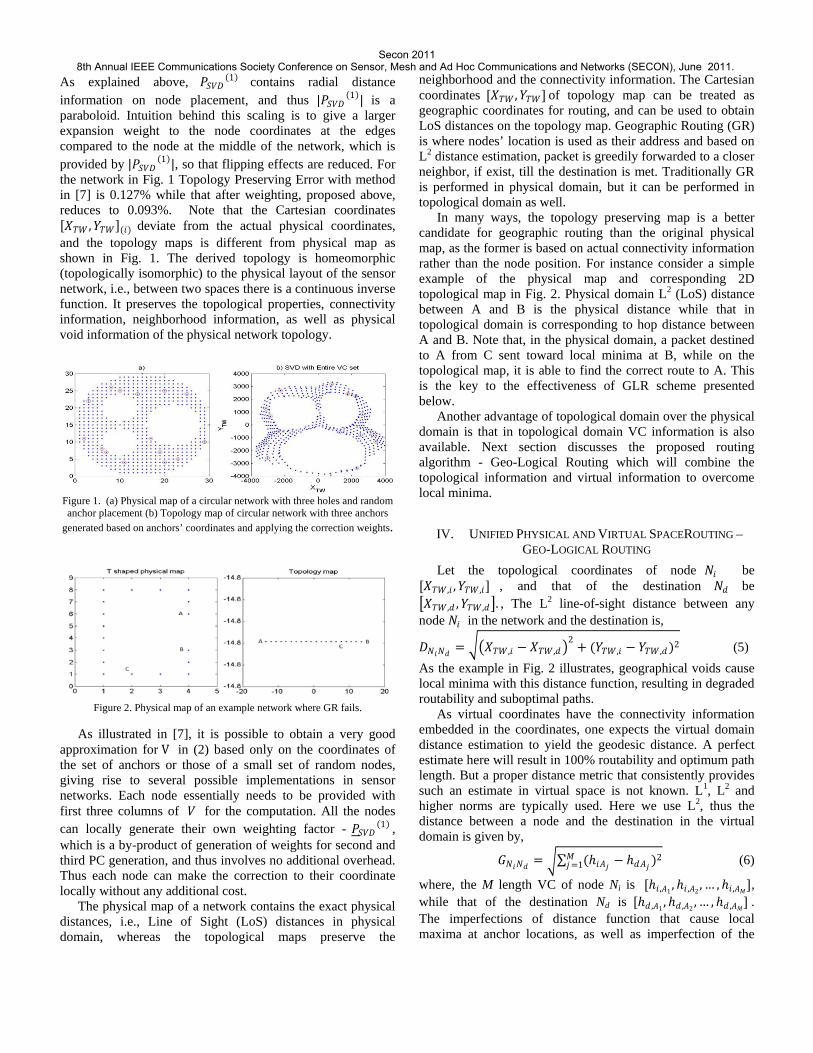
(1)|, so that flipping effects are reduced. For the network in Fig. 1 Topology Preserving Error with method in [7] is 0.127% while that after weighting, proposed above, reduces to 0.093%. Note that the Cartesian coordinates [𝑋𝑋𝑇𝑇𝑇𝑇 ,𝑌𝑌𝑇𝑇𝑇𝑇](𝑖𝑖) deviate from the actual physical coordinates, and the topology maps is different from physical map as shown in Fig. 1. The derived topology is homeomorphic (topologically isomorphic) to the physical layout of the sensor network, i.e., between two spaces there is a continuous inverse function. It preserves the topological properties, connectivity information, neighborhood information, as well as physical void information of the physical network topology.

Figure 1. (a) Physical map of a circular network with three holes and random anchor placement (b) Topology map of circular network with three anchors

generated based on anchors’ coordinates and applying the correction weights.

Figure 2. Physical map of an example network where GR fails.

As illustrated in [7], it is possible to obtain a very good

approximation for V in (2) based only on the coordinates of the set of anchors or those of a small set of random nodes, giving rise to several possible implementations in sensor networks. Each node essentially needs to be provided with first three columns of 𝑉𝑉 for the computation. All the nodes can locally generate their own weighting factor - 𝑃𝑃𝑆𝑆𝑉𝑉𝑆𝑆 (1) , which is a by-product of generation of weights for second and third PC generation, and thus involves no additional overhead. Thus each node can make the correction to their coordinate locally without any additional cost.

The physical map of a network contains the exact physical distances, i.e., Line of Sight (LoS) distances in physical domain, whereas the topological maps preserve the

neighborhood and the connectivity information. The Cartesian coordinates [𝑋𝑋𝑇𝑇𝑇𝑇 ,𝑌𝑌𝑇𝑇𝑇𝑇] of topology map can be treated as geographic coordinates for routing, and can be used to obtain LoS distances on the topology map. Geographic Routing (GR) is where nodes’ location is used as their address and based on L2 distance estimation, packet is greedily forwarded to a closer neighbor, if exist, till the destination is met. Traditionally GR is performed in physical domain, but it can be performed in topological domain as well.

In many ways, the topology preserving map is a better candidate for geographic routing than the original physical map, as the former is based on actual connectivity information rather than the node position. For instance consider a simple example of the physical map and corresponding 2D topological map in Fig. 2. Physical domain L2 (LoS) distance between A and B is the physical distance while that in topological domain is corresponding to hop distance between A and B. Note that, in the physical domain, a packet destined to A from C sent toward local minima at B, while on the topological map, it is able to find the correct route to A. This is the key to the effectiveness of GLR scheme presented below.

Another advantage of topological domain over the physical domain is that in topological domain VC information is also available. Next section discusses the proposed routing algorithm - Geo-Logical Routing which will combine the topological information and virtual information to overcome local minima.

IV. UNIFIED PHYSICAL AND VIRTUAL SPACEROUTING – GEO-LOGICAL ROUTING

Let the topological coordinates of node 𝑁𝑁𝑖𝑖 be [𝑋𝑋𝑇𝑇𝑇𝑇 ,𝑖𝑖 ,𝑌𝑌𝑇𝑇𝑇𝑇,𝑖𝑖] , and that of the destination 𝑁𝑁𝑑𝑑 be �𝑋𝑋𝑇𝑇𝑇𝑇 ,𝑑𝑑 ,𝑌𝑌𝑇𝑇𝑇𝑇 ,𝑑𝑑�. , The L2 line-of-sight distance between any node 𝑁𝑁𝑖𝑖 in the network and the destination is,

𝑆𝑆𝑁𝑁𝑖𝑖𝑁𝑁𝑑𝑑 = ��𝑋𝑋𝑇𝑇𝑇𝑇 ,𝑖𝑖 − 𝑋𝑋𝑇𝑇𝑇𝑇,𝑑𝑑�2 + (𝑌𝑌𝑇𝑇𝑇𝑇,𝑖𝑖 − 𝑌𝑌𝑇𝑇𝑇𝑇 ,𝑑𝑑)2 (5)

As the example in Fig. 2 illustrates, geographical voids cause local minima with this distance function, resulting in degraded routability and suboptimal paths.

As virtual coordinates have the connectivity information embedded in the coordinates, one expects the virtual domain distance estimation to yield the geodesic distance. A perfect estimate here will result in 100% routability and optimum path length. But a proper distance metric that consistently provides such an estimate in virtual space is not known. L1, L2 and higher norms are typically used. Here we use L2, thus the distance between a node and the destination in the virtual domain is given by,

𝐺𝐺𝑁𝑁𝑖𝑖𝑁𝑁𝑑𝑑 = �∑ (ℎ𝑖𝑖𝐴𝐴𝑗𝑗 − ℎ𝑑𝑑𝐴𝐴𝑗𝑗 )2𝑀𝑀

𝑗𝑗=1 (6)

where, the M length VC of node Ni is [ℎ𝑖𝑖,𝐴𝐴1,ℎ𝑖𝑖 ,𝐴𝐴2

, … ,ℎ𝑖𝑖,𝐴𝐴𝑀𝑀], while that of the destination Nd is [ℎ𝑑𝑑 ,𝐴𝐴1

,ℎ𝑑𝑑 ,𝐴𝐴2, … ,ℎ𝑑𝑑 ,𝐴𝐴𝑀𝑀] .

The imperfections of distance function that cause local maxima at anchor locations, as well as imperfection of the


topology maps caused by improper anchor placement result in local minima in logical space. Given that the local minima in physical, topological and virtual spaces are unavoidable, and that we are able to derive topological information from VCs, the proposed Geo-Logical Routing scheme uses one space to overcome the minima in the other space. At local minima, the node changes the routing domain that it is currently operating in (from virtual to topological and vice versa). On rare occasions, when the node is a local minima in both the domains, we use properties of VCS to escape and travel away from that minima. This third phase of routing involves sending the packet to the anchor closest to the destination. The two properties involved are: Property 1: In a connected network of 𝑵𝑵 nodes there is a path between any two nodes via any anchor. Property 1 is self-explanatory. Property 2: In a VCS based system, a packet can be routed from any node to any anchor with 100% routability. Furthermore, the path taken from the node to the anchor is the shortest (optimum path). Proof: Let the ordinate of any node 𝑁𝑁𝑖𝑖 , with respect to the anchor 𝐴𝐴 be ℎ𝐴𝐴. There exists a neighbor to node Ni who has the ordinate of one less, i.e., (ℎ𝐴𝐴 − 1). The new node in turn can find a neighbor a distance (ℎ𝐴𝐴 − 2), and so on, resulting in the packet reaching the anchor in ℎ𝐴𝐴 hops. QED.

The closest anchor to the destination is selected so that the distance from selected anchor to the destination is at its minimum, so the possibility of a local minima occurring in the path from the anchor to destination is minimized.

Closest anchor in hop distance to the destination is determined based on destination’s VC. Since destination’s VC is [ℎ𝑑𝑑 ,𝐴𝐴1 … ℎ𝑑𝑑 ,𝐴𝐴𝑖𝑖 … ℎ𝑑𝑑 ,𝐴𝐴𝑀𝑀 ], the closest anchor to the destination is determined by

𝐴𝐴𝑐𝑐 = argmin𝐴𝐴𝑖𝑖

(ℎ𝑑𝑑 ,𝐴𝐴𝑖𝑖) (7)

A. Geo-Logical Routing Algorithm The routing scheme switches among three modes: TC

which uses topology based coordinates and 𝑆𝑆𝑁𝑁𝑖𝑖𝑁𝑁𝑑𝑑 from (5) for distance; VC which uses virtual coordinates and distance function 𝐺𝐺𝑁𝑁𝑖𝑖𝑁𝑁𝑑𝑑 from (6), and AM, which routes toward selected anchor which is closest to the destination using𝐴𝐴𝑐𝑐 from (7). The source node, initiates routing in TC mode. The packet continues to get routed in this mode until it reaches a local minima in the topology space, at which time the mode is changed to VC mode. If it encounters a local minima in this mode, the packet is routed using the AM mode in which the packet is sent to the anchor closest to the destination. Once the anchor is reached, it goes switches to the VC mode. The algorithm is summarized in Fig. 3. Routing stops when the packet has reached the destination or the TTL expires.

Figure 3. Flow chart of Geo-Logical Routing at a node Ni

while (𝑵𝑵𝒅𝒅 ≠ 𝑵𝑵𝒊𝒊 || 𝑻𝑻𝑻𝑻𝑻𝑻 ≥ 𝟎𝟎 ) if (Mode = = AM ) if 𝑵𝑵𝒊𝒊 = = 𝑨𝑨𝒄𝒄 Set Mode = VC else Send the packet toward the anchor 𝑨𝑨𝒄𝒄 closest to the Destination end else if (Mode = =TC) 𝑹𝑹𝒌𝒌 = 𝑫𝑫𝒋𝒋𝒅𝒅 ; 𝒋𝒋 ∈ 𝑲𝑲;𝑵𝑵𝒋𝒋 ≠ 𝑵𝑵𝒊𝒊,𝑷𝑷𝑷𝑷𝑷𝑷𝑷𝑷,𝑵𝑵𝒊𝒊,𝑵𝑵𝑷𝑷𝑵𝑵𝑵𝑵 % Calculate the topological distance from Neighbors set K to destination excluding 𝑵𝑵𝒊𝒊,𝑵𝑵𝑷𝑷𝑵𝑵𝑵𝑵 and 𝑵𝑵𝒊𝒊,𝑷𝑷𝑷𝑷𝑷𝑷𝑷𝑷 𝒅𝒅𝒋𝒋𝒅𝒅 = 𝑫𝑫𝒋𝒋𝒅𝒅 %Current distance to desination elseif (Mode = = VC) 𝑹𝑹𝒌𝒌 = 𝑮𝑮𝒋𝒋𝒅𝒅 ; 𝒋𝒋 ∈ 𝑲𝑲;𝑵𝑵𝒋𝒋 ≠ 𝑵𝑵𝒊𝒊,𝑷𝑷𝑷𝑷𝑷𝑷𝑷𝑷,𝑵𝑵𝒊𝒊,𝑵𝑵𝑷𝑷𝑵𝑵𝑵𝑵 % Calculate the virtual distance from Neighbors set K to destination excluding 𝑵𝑵𝒊𝒊,𝑵𝑵𝑷𝑷𝑵𝑵𝑵𝑵 and 𝑵𝑵𝒊𝒊,𝑷𝑷𝑷𝑷𝑷𝑷𝑷𝑷 𝒅𝒅𝒋𝒋𝒅𝒅 = 𝑮𝑮𝒋𝒋𝒅𝒅 end if 𝑹𝑹𝒌𝒌= ={} %If there is no neighbor excluding 𝑵𝑵𝒊𝒊,𝑷𝑷𝑷𝑷𝑷𝑷𝑷𝑷,𝑵𝑵𝒊𝒊,𝑵𝑵𝑷𝑷𝑵𝑵𝑵𝑵 Set Mode= AM % Shift to Anchor Mode else if 𝑴𝑴𝒊𝒊𝑴𝑴(𝑹𝑹𝒌𝒌) == 𝟎𝟎 if 𝑵𝑵𝒅𝒅 == 𝑵𝑵𝒊𝒊 ROUTED else % if identical coordinates switch Mode % current mode at a minima case VC Set Mode=TC % Shift to Topology based GF case TC Shift to Anchor Mode Set Mode= AM end end elseif 𝑴𝑴𝒊𝒊𝑴𝑴(𝑹𝑹𝒌𝒌) ≤ 𝒅𝒅𝒊𝒊𝒅𝒅 𝑵𝑵𝒊𝒊,𝑷𝑷𝑷𝑷𝑷𝑷𝑷𝑷 = 𝑵𝑵𝒊𝒊

𝑵𝑵𝒊𝒊 = 𝒂𝒂𝑷𝑷𝒂𝒂𝒂𝒂𝒊𝒊𝑴𝑴

𝒋𝒋 𝑹𝑹𝒌𝒌(𝒋𝒋)

𝑵𝑵𝒊𝒊,𝑵𝑵𝑷𝑷𝑵𝑵𝑵𝑵 = 𝒂𝒂𝑷𝑷𝒂𝒂𝒂𝒂𝒊𝒊𝑴𝑴

𝒋𝒋 𝑹𝑹𝒌𝒌(𝒋𝒋)

elseif 𝑴𝑴𝒊𝒊𝑴𝑴(𝑹𝑹𝒌𝒌) > 𝒅𝒅𝒊𝒊𝒅𝒅 %Local minima switch Mode % current mode at a minima case VC Shift to Topology based GF Set Mode=TC case TC Shift to Anchor Mode Set Mode= AM end end end end end

Figure 4. Pseudo code of GLR algorithm.


It is important to note that many variations of this algorithm are possible, such as moving only a certain distance toward closest anchor in AM mode before switching, or switching between TC and VC modes more frequently or probabilistically. The particular algorithm considered in this paper produces significant performance gains with a straight forward switching mechanism.

B. Local Minima Identification in the Algorithm A node identifies itself as local minima in physical or

virtual domain if its distance to the destination is lower than the distances from each of its neighbors to the destination. Distance evaluation is performed based on the current mode of routing. If the packet is routed based on topological coordinates of the node then the local minima is identified by, 𝑆𝑆𝑁𝑁𝑐𝑐𝑁𝑁𝑑𝑑 < 𝑆𝑆𝑁𝑁𝑖𝑖𝑁𝑁𝑑𝑑 ,∀𝑁𝑁𝑖𝑖 ∈ 𝐾𝐾 , where 𝑆𝑆𝑁𝑁𝑐𝑐𝑁𝑁𝑑𝑑 , and 𝑆𝑆𝑁𝑁𝑖𝑖𝑁𝑁𝑑𝑑 are distance from current node to destination and neighbor(s) to destination based on topological coordinates. If the mode is VC based routing then the packet is at a local minima if, 𝐺𝐺𝑁𝑁𝑐𝑐𝑁𝑁𝑑𝑑 < 𝐺𝐺𝑁𝑁𝑖𝑖𝑁𝑁𝑑𝑑 ,∀𝑁𝑁𝑖𝑖 ∈ 𝐾𝐾 , where 𝐺𝐺𝑁𝑁𝑐𝑐𝑁𝑁𝑑𝑑 , and 𝐺𝐺𝑁𝑁𝑖𝑖𝑁𝑁𝑑𝑑 are distance from current node to destination and neighbor(s) to destination based on VCs. Exact destination is identified by unique node IDs.

In the proposed routing scheme a node saves the predecessor and successor node information in order to avoid having loops. The packet header contains a field that indicates the current mode of routing (TC, VC or AM). The algorithm is specified in detail in Figure 4.

V. PERFORMANCE OF GLR The performance of GLR is evaluated next, and compared

with two virtual coordinates based routing schemes - Logical Coordinate Routing (LCR) and Convex Subspace Routing (CSR) - and the geographic routing scheme Greedy Perimeter Stateless Routing (GPSR).

A. Evaluation Method

We use the four example networks shown in Fig. 5 that are representative of a variety of networks. The number of nodes range from 300 to 800. MATLAB® 2009b based simulator was used for the computations. In selecting options for the different protocols, we have favored the competitor schemes so that we can demonstrate the effectiveness of GLR even under such conditions. The physical topologies in Fig. 5 have four or less number of neighbors in a grid like placement, and the communication range of a node in all four networks is set to unity. This placement highly favors the GPSR scheme since the grid like placement reduces looping and supports the right hand rule based local minima overcome method. For example, the circular network with holes can be significantly warped if more random transmission ranges are allowed, and many such cases will introduce other concave physical voids that need to be overcome. The transmission distance on the other hand has no effect on the topology preserving map, thus all such implementations correspond to the same topology map. Therefore the performance would remain unchanged in GLR.

Note also that the spiral in Figure 5(a) favors the right hand rule of GPSR, i.e., GPSR performance will deteriorate drastically on a spiral shape winding in the opposite direction.

Figure 5. (a) Spiral shaped network of 421 nodes; (b) Circular network of 496 nodes with three holes; (c) A 30 by 30 node grid with 100 randomly missing nodes; and (d) Network of 343 nodes deployed on walls of a building. Red

stars indicate anchors with manual anchor placement. In LCR implementation, we assumed that the entire path traversed is available at each node so that backtracking can be perfectly performed avoiding any loops; i.e., the implemented case is the best case of LCR, and is not achievable in practice due to the cost involved in transmitting the required information. Time-To-Live (TTL) of the packet is set to 100 hops. The performance of logical routing schemes and the accuracy of topology maps are dependent on the anchor placement. Two anchor placement strategies are used for the evaluation: random anchor placement and manual anchor placement. In the former, a randomly selected set of nodes serves as anchors, with the number of anchors varied from 5 to 20. As different random placements of the same number of anchors result in different performances, the value averaged over five different random placements is provided together with maximum and minimum performances indicated as error bars in the plots. In manual anchor placement, four anchors were placed at locations selected based on our intuition about how anchors should be placed. It did not involve any evaluation, iterative efforts, or complex decisions to assure its optimality, and therefore they should be considered only as indicative of what can be expected with a good anchor placement strategy. Such placements should be realizable in practice using good placement algorithms. The red nodes in Fig. 5 are the manually placed anchors.

Average routability and average path length that packets traversed are used as the performance metrics. Average routability evaluation considers all source-destination pairs; i.e., each node generated a set of (N-1) messages, with one message for each of the remaining node as the destination. Average routability =

Total # of packet that reached the destinationTotal number of packet generated

(8)


Average path length = Cumilative number of hops that each packet traversed

Total number of packet generated (9)

Note that the average path length calculation includes the path lengths for unrouted messages as well.

As outlined in Section III and [7], three options differing complexity and accuracy are available for 𝑃𝑃 for computing 𝑃𝑃𝑆𝑆𝑉𝑉𝑆𝑆 in Eqn. (2): a) 𝑃𝑃 is the 𝑁𝑁 × 𝑀𝑀 based on entire set of VCS, b) it is the 𝑀𝑀 × 𝑀𝑀 matrix based on anchor’s coordinates only, and c) 𝑃𝑃 is an 𝑅𝑅 × 𝑀𝑀 matrix based on a random set of 𝑅𝑅 node coordinates. The first it the most complex, in terms of the computation and communication cost. When the number of random nodes selected is less than the number of anchors, c) is the most efficient. We use this simplest and most computationally and communication wise efficient option with only the coordinates of ten (𝑅𝑅 = 10) randomly selected nodes.

B. Effectiveness of Physical and Topology based Cartesian

Coordinates in Packet Forwarding In Section III we asserted that in many ways, the topology

preserving map is a better candidate for geographic routing than the original physical map, as the former is based on actual connectivity information rather than the node position. If this is the case, it is extremely significant as topology based coordinates can be generated much more easily, efficiently and economically compared to obtaining the physical locations. A set of coordinates is better for routing if it results in more accurate forwarding decisions. This can be quantitatively evaluated using P[Selecting correct neighbor] =

∑# number of times a node selected correct node

to FWD the packet when destination is NiTotal # nodes (N)Ni∈N (10)

TABLE II. PROBABILITY OF SELECTING THE CORRECT NEIGHBOR BASED ON TOPOLOGY COORDINATES AND PHYSICAL COORDINATES FOR THE

NETWORKS IN FIG. 5

Probability of Selecting Correct Neighbor Network Topology

Topology Coordinates Physical Coordinates M=20 M=15 M=10 M=5 M=4*

Fig. 5 (a) 0.66 0.63 0.63 0.65 0.66 0.43 Fig. 5 (b) 0.64 0.61 0.62 0.52 0.54 0.54 Fig. 5 (c) 0.64 0.64 0.6 0.56 0.65 0.61 Fig. 5 (d) 0.84 0.80 0.78 0.72 0.84 0.83 * Manually placed 4 anchors

Table 2 shows the probability of a node selecting the correct neighbor to forward the packet based on L2 distance metric using physical and topology based Cartesian coordinates. The results clearly indicate that topology-based coordinates are more effective (or as effective in the worst case), in selecting the correct neighbor to forward the packet in greedy forwarding compared to physical coordinates. This is a remarkable result, which indicates that expensive localization procedures are unnecessary for the purpose of routing packets or other self-organization tasks.

Several factors have to be taken into account to understand the significance of topological coordinates, and the fact that it is not just a substitute for physical coordinates, rather that it is a

significantly better option for routing and self-organization. Topology maps generated with 10 randomly selected anchors has the capability of selecting the correct next neighbor as accurately as with physical coordinates for the networks ranging from 340 to 800 nodes. With strategically placed anchors, better performance was demonstrated with as few as 4 anchors. The cost of generating the topological coordinates is significantly lower than that to generate a physical map. Generating VCs involve a single flooding for each anchor, and each collecting coordinates from a set of small number of random nodes. Physical localization in contrast depends on analog measurements. Signal strength measurements require specific hardware capabilities at each node, while time delay requires accurate clock synchronization. Analog measurements have to be repeated to obtain reliable estimates, and are susceptible to noise, fading and even battery level. The errors propagate cumulatively with localization algorithms. It has been demonstrated elsewhere that even a small error and ignoring the impact of errors of location information has a drastic effect on routability. For example, with Geographic Routing- GEAR [24] the routability performance falls below 50% when the distances estimation inaccuracy is 6% [17]. Also, note that we have used a regular grid based placement and perfect location estimates that are very favorable to routing using physical coordinates. These considerations have significantly biased the results in favor of the physical coordinates, and the values are likely to much less favorable under more realistic conditions.

C. Performance of GLR with Random Anchor Placement

Now we evaluate and compare the performance of GLR with existing logical schemes (LCR and CSR) and geographic routing scheme (GPSR). Random anchor placement was used for logical routing schemes. GPSR performance is independent of the number of anchors as it is based on physical coordinates. Also, as manual anchor placement used for GLR-M relied only on four anchors, the X-axis is not applicable for GLR-M either. Fig. 6 and 7 show the routability and the path lengths respectively, averaged over five placements of random anchors. Note that GLR outperforms LCR, CSR and GPSR in Circular network with three holes, Spiral network and in the grid with missing nodes in terms of average routability and path length when there are more than 10 randomly placed anchors in the network. Based on results from Section B, one can expect similar or better performance from GLR with a smaller number of anchors with a proper anchor placement. The performance for the case when there are exactly 10 anchors is summarized in Table III. Note that the average path length includes path length traversed even for packets not routed correctly. LCR for example, discards the packets when it cannot route it further, resulting in smaller contribution toward path length, even though the actual path length is much higher. Higher routing percentages can be achieved only by routing such difficult packets, resulting in longer average path length. The shortest path corresponds to an ideal routing scheme. In the building network, GLR out performs LCR and CSR by 40 % in each with 5 anchors, 40% and 15% with 10 anchors; 30% and 15% with 15 and 20 anchors; respectively. Only in the building network is the performance of GPSRs better than with GLR.


Figure 6. Average Routability of GLR with random and manual anchor placement (GLR-R,GLR-M respectively), LCR, CSR and GPSR in (a) Spiral network, (b) Circular network with 3 holes, (c) Grid with 100 missing nodes, and (d) Network in a building.

It achieves 97.3% routability, vs. 89.3% for GLR, with an average to shortest path length ratio of 1.4, vs. 1.5 for GLR. Note in this case, the topology is very regular. As the number of anchors is increased the routability of GLR increases by ~10% in grid with 100 missing nodes, spiral and network in the building, while that in circular network with holes is 23%.

D. Performance of GLR with Manual Anchor Placement With manually placed anchors, more accurate topology maps are achievable with a very low number of anchors. Thus GLR-M achieves higher routability with low path length as shown

Figure 7. Average path length of GLR with random and manual anchor

placement (GLR-R,GLR-M respectively), LCR, CSR and GPSR in (a) Spiral network, (b) Circular network with 3 holes, (c) Grid with 100 missing nodes,

and (d) Network in a building.

in Fig. 6 and 7. As summarized in Table IV, GRL-M achieves routability near 98 % for the circular network with three holes and grid with missing nodes, with path length to shortest path length ratio of 1.4 and 1.2 respectively. Achieving routability of 92.4% and 93.4% for spiral network and network in the building correspondingly with only 4 anchors and a path length 1.5 and 1.2 times with respect to shortest path length is remarkable. Table V indicates that packets are forwarded by GLR in the TC mode most of the time (72-86%), in VC mode 7-18% of the time and in AM less than 10% of the time.


TABLE III. PERFORMANCE COMPARISSION BETWEEN GLR, LCR, CSR AND GPSR WITH 10 ANCHORS

Topology – Figure 5 Performance Parameter Spiral

Circle with voids

Grid with holes

Building network

% of nodes as anchors 2.4 2.0 1.25 2.9 Routability

Avg. routability GLR 93.9 94.6 93.4 89.3 Avg. routability LCR 57.5 56.5 60 49.7 Avg. routability CSR 89.2 87.3 84.3 75.4 Avg. routability GPSR 49.1 93.8 89.6 97.4 Path Length

Actual path length 36.1 20.3 20.7 22.8 Avg. path length GLR 41.8 28.3 28.1 34.1 Avg. path length LCR 25.9 15 16.3 15 Avg. path length CSR 43.7 26 26 26.4 Avg. path length GPSR 59.8 50.1 21.8 32.7

TABLE IV. PERFORMANCE OF GLR WHEN FOUR ANCHORS ARE STRATERGICALLY PLACED (GLR-M)

Topology Fig. 5

Avg. Routability %

Avg. Path Length

Path length/Shortest Path Length

Spiral 93.42 42.1 1.2 Circle with voids 98.49 28.5 1.4 Grid with holes 97.7 25.2 1.2

Building network 92.4 33.3 1.5

TABLE V. ACTIVE PERCENTILE OF EACH MODE IN ROUTING

Topology Fig. 5

Topological Coordinate mode

Virtual Coordinate mode

Anchor Mode

Spiral 79.4% 12.7% 7.9% Circle with voids 86.0% 7.0% 7.0% Grid with holes 75.0% 17.9% 7.1%

Building network 72.6% 17.7% 9.7%

VI. CONCLUSION AND FUTURE WORK Geo-Logical Routing is the first scheme to combine the

advantages of logical and geographic routing techniques. It uses topological coordinates obtained from Virtual Coordinates and virtual coordinate based routing to overcome the deficiencies associated with local minima problem in physical and logical domains. Cartesian coordinate estimation is based on an algorithm that uses the second and third dominant principal component of logical coordinates to produces a topology map, which then is scaled using the first component. Topology based Cartesian coordinates so derived are more effective for geographic routing than the physical geographical coordinates. This is because topological maps preserve neighborhood information as well as connectivity information. Even under conditions favorable to physical coordinate based routing, i.e., no localization errors and grid like node placement, GLR outperforms GPSR in 3 out of 4 complex network topologies. A building network where the GPSR performance seems to be better than GRL is one very favorable for geometric routing; still GRL routability without localization and with only 4 anchors there is noteworthy.

The novel concept of combining topological domain routing and virtual domain routing opens the path for designing novel adaptive routing protocols that operate in multiple coordinate domains. Improved anchor placement strategies can further improve the routing effectiveness. It is important to note that many variations of GLR algorithm can be developed, such as moving only a certain distance toward the closest anchor in

AM mode before switching, or switching between TC and VC modes more frequently, probabilistically, or based on an adaptive scheme. Evaluation of such generalized GLR strategies is part of the ongoing work.

REFERENCES [1] J.N. Al-Karaki, and A.E. Kamal, “Routing techniques in wireless sensor

networks: a survey,” IEEE Wireless Communications, Vol. 11, pp.6-28, Dec. 2004.

[2] J. Bachrach and C. Taylor, "Localization in sensor networks," Ch. 9, Handbook of Sensor Networks, Stojmenovic (Editor), John Wiley 2005.

[3] A. Caruso, S. Chessa, S. De, and A. Urpi, “GPS free coordinate assignment and routing in wireless sensor networks,” Proc. 24th IEEE Joint Conf. of Computer and Communications Societies, Vol. 1, pp. 150- 160, March 2005.

[4] Q. Cao and T Abdelzaher, “Scalable logical coordinates framework for routing in wireless sensor networks”, ACM Transactions on Sensor Networks,Vol. 2,No. 4,pp. 557-593, Nov 2006.

[5] D.C. Dhanapala, Q. Han and A.P. Jayasumana, “Performance of random routing on grid-based sensor networks,” Proc. IEEE Consumer Communications and Networking Conference (CCNC), Jan. 2009.

[6] D. C. Dhanapala and A. P. Jayasumana, "CSR: convex subspace routing protocol for WSNs,"Proc. 34th IEEE Conf. on Local Computer Networks, Oct. 2009.

[7] D.C. Dhanapala and A.P. Jayasumana, “Topology preserving maps from virtual coordinates for wireless sensor networks,” 35th IEEE Conf. on Local Computer Networks (LCN), Oct. 2010.

[8] Q. Fang, J. Gao and L.J. Guibas, “Locating and bypassing routing holes in sensor networks,” Proc. IEEE INFOCOM, pp. 2458–68, vol.4, 2004.

[9] W. Jia, T. Wang, G. Wang and M. Guo, “Hole avoiding in advance routing in wireless sensor networks,” Wireless Communications and Networking Conference(WCNC), pp. 3519 – 3523, 2007.

[10] B. Karp and H.T. Kung, “GPSR:Greedy perimeter stateless routing for wireless networks,” Proc. 6th ACM/IEEE Int. Conf. Mobile Computing and Networking (MobiCom 2000), pp. 243-254,August, 2000.

[11] E. Kranakis, H. Singh and J. Urrutia, “Compass routing on geometric networks,” Proc. 11th Canadian Conf. on Computational Geometry, Vancouver, Aug. 1999.

[12] B. Leong, S. Mitra, and B. Liskov, “Path vector face routing: Geographic routing with local face information,” Proc. 13th IEEE Int. Conf. on Network Protocols (ICNP'05), 2005 .

[13] C-H Lin, B-H Liu, H-Y Yang, C-Y Kao, and M-J Tsai, “Virtual-coordinate-based delivery-guaranteed routing protocol in wireless sensor networks with unidirectional links”, Proc. IEEE INFOCOM 2008,pp: 351-355, April 2008.

[14] K. Liu and N. Abu-Ghazaleh , “Aligned virtual coordinates for greedy routing in WSNs,” Proc. IEEE Int. Conf. on Mobile Adhoc and Sensor Systems, pp. 377–386, Oct. 2006.

[15] K. Liu and N. Abu-Ghazaleh, “Stateless and guaranteed geometric routing on virtual coordinate systems,” Proc. 5th IEEE Int. Conf. Mobile Ad Hoc and Sensor Systems( MASS 2008). pp. 340-346, Oct. 2008.

[16] H.A.B.F. Oliveira, E. F. Nakamura, A. A. F. Loureiro, and A. Boukerche, “Error analysis of localization systems for sensor networks,” Proc. 13th ACM Int. Wkshp on Geographic Information Systems, Germany, pp. 71 – 78, 2005.

[17] A. Rao, S. Ratnasamy, C. Papadimitriou, S. Shenker, and I. Stoica ,“Geographic routing without location information,” , Proc. 9th Int. Conf. on Mobile Computing and Networking, pp. 96 - 108, 2003.

[18] L. Shu, Y. Zhang, L.T. Yang, Y. Wang and M. Hauswirth, “Geographic Routing in Wireless Multimedia Sensor Networks,” 2nd Int. Conf. Future Generation Commun. & Networking (FGCN),pp. 68 – 73, 2008.

[19] M. J. Tsai, H. Y. Yang, and W. Q. Huang, “Axis based virtual coordinate assignment protocol and delivery guaranteed routing protocol in wireless sensor networks,” Proc. INFOCOM,pp: 2234-2242, 2007 .

[20] Y. Yu, R. Govindan and D. Estrin, “Geographical and Energy Aware Routing: A recursive data dissemination protocol for WSNs,” UCLA CS Dept Tech. Rept., UCLA/CSD-TR-01-0023, May 2001.


Documents

Secon 2011 Geo-Logical Routing in Wireless Sensor Networks*