Embed Size (px)
Citation preview

SECA-FR-95-08
ZERO SIDE FORCE VOLUTE DEVELOPMENT
Contract No. NAS8-39286
Final Report
Prepared for:
National Aeronautics & Space Administration
George C. Marshall Space Flight Center
Marshall Space Flight Center, AL 35812
P. G. Anderson, R. J. Franz, R. C. Farmer
Y. S. Chen ( _
(Engineering Sciences, Inc.)
SECA, Inc.3313 Bob Wallace Avenue
Suite 202
Huntsville, AL 35805
p,..
t'q
4:)
,-4
I
Z
0
¢r_ ,,..,.
0
C9 C
u) L,L
Z
Lij
O" _..
,.-4 C3 '...1.
0 _
I _J _-_
c_ C_
_J
I L..JP_
_ I-- c:
Z _L_ t_
t_
t--
,0
CO
00
https://ntrs.nasa.gov/search.jsp?R=19960009112 2020-01-03T16:46:48+00:00Z

- SECA-FR-95-08
ACKNOWLEDGMENTS
These investigators wish to thank Dr. Paul McConnaughey and Mr. Robert Garcia of
NASA Marshall Space Flight Center (MSFC), the technical monitors of this study, for their
interest and encouragement in this research and Mr. Heinz Struck, formerly of MSFC, for
initiating this investigation. Our appreciation to: Prof. Chris Brennen of California Institute
of Technology and his student Mr. Robert Uy for successfully accomplishing the experimental
portion of this research, Mr. Tom Tyler for his careful mechanical design and construction of
the test volute, Prof. Bharat Soni and Robert Wy of Mississippi State University, and Mr. Ted
Benjamin of MSFC for preparing IGES grid files.
SECA-FR-95-08
SUMMARY
Collector scrolls on high performance centrifugal pumps are currently designed with
methods which are based on very approximate flowfield models. Such design practices result
in some volute configurations causing excessive side loads even at design flowrates. The
purpose of this study was to develop and verify computational design tools which may be used
to optimize volute configurations with respect to avoiding excessive loads on the bearings.
The new design methodology consisted of a volute grid generation module and a
computational fluid dynamics (CFD) module to describe the volute geometry and predict the
radial forces for a given flow condition, respectively. Initially, the CFD module was used to
predict the impeller and the volute flowfields simultaneously; however, the required
computation time was found to be excessive for parametric design studies. A second
computational procedure was developed which utilized an analytical impeller flowfield model
and an ordinary differential equation to describe the impeller/volute coupling obtained from the
literature, Adkins & Brennen (1988). The second procedure resulted in 20 to 30 fold increase
in computational speed for an analysis.
The volute design analysis was validated by postulating a volute geometry, constructing
a volute to this configuration, and measuring the steady radial forces over a range of flow
coefficients. Excellent agreement between model predictions and observed pump operation
prove the computational impeller/volute pump model to be a valuable design tool. Further
applications are r_ommended to fully establish the benefits of this new methodology.
ii

SECA-FR-95-08
TABLE OF CONTENTS
ACKNOWLEDGEMENTS
SUMMARY
TABLE OF CONTENTS
NOMENCLATURE
1.0 INTRODUCTION
1.1 Overview
1.2 The Nature of the Problem
2.0 VOLUTE GRID GENERATION
3.0 CFD RESULTS
3.1 The FDNS CFD Impeller/Volute Pump Model
3.2 2-D Volute Simulation
3.3 3-D CFD Simulation of Volute A
3.3.1 CFD Simulation of Both Volute A and Impeller X
3.3.2 CFD Simulation of Volute A using Adkins/Brennen's
Model for Impeller X
4.0 DESIGN OF A TEST VOLUTE
4.1 Parametric Studies
4.2 Selection of the Test Volute
5.0 EXPERIMENTAL EVALUATION OF TEST VOLUTE
6.0 CONCLUSIONS
7.0 RECOMMENDATIONS
REFERENCES
APPENDIX A
A.1
A.2
A.3
APPENDIX
APPENDIX
The Adkins/Brennen Impeller/Volute Interaction Model
Caltech Pump Test Data from Previous Studies
Instructions for Using Adkins.for
B: Radial Force Measurements for the SECA Volute
C: Operational Instructions for the Volute Geometry Generation Code
i
ii
..,
111
iv
1
1
2
8
18
18
22
28
28
37
43
43
49
55
59
60
61
62
62
67
75
B-1
C-1
.°.
111

SECA-FR-95-08
NOMENCLATURE
Cp static pressure coefficient
Cv function of the moments of the cross-sectional area
C1,C2,C3 turbulence modeling constants
Dp
d
F
F{t}
Fox
Foy
Fx
Fy
G_jh
J
k
Pi
Pr
P
qR
r
SqAS
S
t
Ui
Ui
V
V
x
YZ
_1 _E2_63
3,
/z
turbulence modeling constant
pressure coefficient at volute inlet
numerical dissipation terms of the discretized governing equations
numerical fluxes in the G-direction of the discretized governing equations
integration constant in Bernoulli's equation
steady fluid force acting on the impeller in the x-coordinate direction for a minimum
force spiral volute
steady fluid force acting on the impeller in the y-coordinate direction for a minimum
force spiral volute
steady fluid force acting on the impeller in the x-coordinate direction
steady fluid force acting on the impeller in the y-coordinate directiondiffusion metrics
total head (h" = 2h/pfl2R22)Jacobian of coordinate transformation
turbulence kinetic energy
pressure in impeller
turbulent kinetic energy production rate
static pressure
flow primitive variables
impeller radius
radial component of polar coordinate system
source terms of the governing equations
cross-section area of a control volume perpendicular to the flux vector
length in tangential direction
time
volume-weighted contravariant velocities
flow velocity components in cartesian coordinate
velocity in volute
relative flow velocity in impellercartesian coordinate in the direction from volute center to volute tongue
cartesian coordinate in the direction normal to the x-coordinate
cartesian coordinate
relaxation parameter of the pressure correction equation
perturbation function for impeller flow (in Appendix A)
turbulent kinetic energy dissipation rate
distance between impeller and volute centers (in Appendix A)
e/R2 (in Appendix A)
coefficients of the numerical dissipation terms
flow coefficient
angle of flow path through impeller
effective viscosity
iv

SECA-FR-95-08
/,tl
kttf_
60
1,p
_q0
_,_,_
fluid viscosity
eddy viscosity
radian frequency of the impeller (shaft) rotation
radian frequency of the circular whirl orbittotal head rise coefficient
fluid density
turbulence modeling constant
angular component of polar coordinate system
coordinates of computational domain
Subscripts
C
expi
0
S
x,y,z
1
2
component of cos(oJt)
experimental result
location of a grid pointcentered impeller value (nondimensionalized)
component of sin(wt)
partial derivative components in the cartesian coordinate
impeller inlet
impeller discharge
Superscripts
n variables at previous time step
n+ 1 variables at current time step' correction value
" measurement made from frame fixed to rotating impeller
* nondimensionalized quantity
V

- SECA-FR-95-08
1.0 INTRODUCTION
1.1 Overview
Collector scrolls on high performance centrifugal pumps are currently designed with
methods which are based on very approximate flowfield models. Such design practices result
in some volute configurations causing excessive side loads even at design flowrates. The
purpose of this study was to develop and verify computational design tools which may be used
to optimize volute configurations with respect to avoiding excessive loads on the bearings.
The Space Shuttle Main Engine's (SSME) High Pressure Fuel Turbopump (HPFTP)
experiences such large side loads, that even after a short running time, the useful life of the rotor
bearings is consumed and the bearings require replacement. While impeller/volute interactions
produce side loads, current opinion is that the excessive side loads that require frequent bearing
replacement is the result of other influences. The High Pressure Oxidizer Turbopump also
experienced high side loads, which was a factor in the Alternate Turbopump Development
(ATD). The ATD indeed produced very low side loads, but it was found that purposely
increasingly these side loads improved the operation of the pump. Fluid film bearings are
currently being strongly considered for turbopump application. The use of fluid bearings
increases concern over rotordynamic effects. All of these concerns are benefited by an increased
understanding of impeller/volute coupling effects caused by geometry and flowfield interactions.
Thus, the ability to computationally simulate turbopumps more accurately would advance pump
technology required for launch vehicle design.
The computational impeller/volute pump model was developed by creating three modules:
. A grid generation code was written to expedite the accurate specification of the volute
geometry with a small number of adjustable parameters.
. A state-of-the-art computational fluid dynamics (CFD) code, FDNS, was used to simulate
a fully coupled impeller/volute interaction and to determine side forces caused by the
SECA-FR-95-08
pump operation.
. An existing analytical model developed by Adkins and Brennen (1988) was used to
represent the impeller flow and the interaction between the impeller and the volute
flowfields. This module was developed to affect an improvement in computational
efficiency over the fully coupled impeller/volute CFD model.
These three modules constitute an accurate and practical code to design volute configurations.
Existing test data and experimental tests conducted at Caltech as part of this study were used to
provide verification for the computational impeller/volute pump model.
This report describes the development of these modules and their verification. The
format of the presentation shall be: a brief summary of impeller/volute behavior, a description
of volute grid generation, results of CFD simulations of impeller/volute flows, the design of a
test volute, and the experimental verification of the performance of the test volute.
1.2 The Nature of the Problem
To eliminate the side forces on the pump bearings, the imbalance of radial forces created
by the non-axisymmetric discharge conditions of the impeller flow into the volute must be
eliminated. Currently, high performance centrifugal pump design is not performed by using
CFD methodology. The analytical methodology which is utilized is typified by the analysis of
Adkins and Brennen (1988), in which the interactions that occur between a centrifugal pump
impeller and a volute are described with approximate analytical models. Treatments of the
inability of blades to perfectly turn the flow through the impeller and of quasi-one dimensional
flow through the volute are the major elements of this analysis. Since this study involves design
concepts, the understanding of pump operation derived from previous experimental studies will
be reviewed to establish the basis for future model development.
The design of the SSME turbopumps follows the trend toward higher speed and higher
power density turbomachinery which creates a greater sensitivity to operational problems. This
2

SECA-FR-95-08
studyfocusedon the steady, radial forces acting on the impeller and its bearings due to the flow
through the pump diffuser and volute. Even though the SSME HPFTP has three stages,
attention was directed to a single stage pump so that a meaningful point of departure for CFD
design tool development can be established. Using present design methods, radial side loads can
be minimized for design flow rates for a single stage pump by properly matching an impeller
and volute, as illustrated in Fig. 1 taken from Chamieh (1983). For the configuration shown,
the design condition occurs when the flow coefficient has a value of 0.092. A recent account
of fluid induced impeller forces is presented by Brennen (1994). However, such forces are not
zero if design flowrates are not realized and if inlet flows are not ideal, as would be the case if
the inlet flow were from a previous stage.
The steady impeller fluid force components, Fox and Foy, shown in Fig. 1 are defined in
terms of a coordinate system in which x is the coordinate defined by the impeller centerline and
the volute cutwater (tongue); y is normal to x in the direction of the impeller rotation. Fox is
nearly optimum since it is very small over a wide range of flowrates about the design point.
The behavior of Foy is much more difficult to optimize since it varies from large positive values
to large negative values as the flow coefficient varies through the design flow condition. This
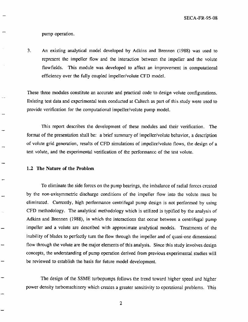
point is emphasized by plotting the magnitude of the impeller force, Fo, as shown in Fig. 2,
Chamieh (1983). Fo is not zero, but it is a minimum for the spiral volute (volute A) when Foy
passes through zero, i.e. the design point. To eliminate the side forces, Fox and Foy must
simultaneously be zero. The best one could hope for is to design the volute/diffuser such that
the "sweet-point" in the curve shown in Fig. 2 is close to zero for a wide range of flowrates
about the design point. Hence, the design goal for selecting volute/diffuser configurations is to
make the behavior of Foy approach that of Fox in a plot such as that shown in Fig. 1. The CFD
model volute flow developed in this study was used to investigate conditions under which such
desired behavior can be obtained.
The influence of volute shape is also shown in Fig. 2 by a comparison of a spiral volute
to a circular volute (volute B), presented by Chamieh (1983). Volute B becomes the optimum
shape as the flow coefficient approaches zero, as evidenced by this figure. This qualitative
effect is typical of the predictive behavior which any CFD model must exhibit to be useful as

- SECA-FR-95-08
i,i
N_ -0.06-_I
:Er,- -0.080Z
0
I I I I I I I
o"
VOLUTE B, Foly_
(800: O', IZOO:<>) _0 -
I I 1 I I I I0.02 0.04 0.06 0.08 0.10 0.12 0.14
A0
_ a(> or,z_o
0"<>c_
FLOW COEFFICIENT, (_
Fig. 1 Normalized average volute force components are shown for Impeller X, Volutes A and
B and for face seal clearances of 0.79 ram. Rotor speeds in rpm and their corresponding
symbols are shown in brackets, from Chamieh (1983)
4
- SECA-FR-95-08
0.1-8
0.16
I-Z 0.1'_bJ
0LI.IJ."' 0.120(J
0r,. o.Foou.
LUI-- 0.08
_JO>
,,, 0.06(.9
n-LU
> O.04
.c}laJN"i 0.02,¢(
n-OZ
0
I I I I I
0
0
Z_
ZS
0,I
I I
SHAFT RPM
600
800
I 200
f VOLUTE A(LOG SPIRAL)
E" VOLUTE B Z_ -
_,CIRCULAR)
4,$ o
• .ZS ZS -0
I I ! I I I I0.02 0.04 0.06 0.08 0-10 0.12 0.14
FLOW COEFFICIENT,
Fig. 2 Normalized average volute force for Impeller X and face seal clearances of 0.79 ram.
Open and closed symbols represent data for Volutes A and B respectively, from Chamieh(1983).
5

SECA-FR-95-08
a designtool for centrifugalpumps.
Experimentalstudieshavealsobeenconductedto optimizevolute configurations.Figure
3 from Agostinelli, et al (1960)showstheeffecton theradial forcesof usinga volute which is
initially circular and then becomesspiral, as the flow progressesfrom the cutwater to the
discharge.This figure alsoshowstheeffectof usinga doublevolute, which is nearly ideal for
reducingradial forcesat all flow rates. However, other designpenalties,suchas additional
weightand structuralcomplexityin geometricallysmall pumps,precludethe usefulnessof this
configuration. A vaneddiffuserbetweentheimpeller andthevolute mayalsobeusedto reduce
radial forces, but, again, at the expenseof introducing other complications. This study
addressedonly the improvementof volute shapefor controlling sideloads.
Severalother very important factorsalsocontributeto radial forces: (1) thosedue to
whirl causedby the impellerbeingdisplacedfrom the "design"centerof thevolute (becauseof
shaft wear, bearing wear, tolerances,etc.), (2) thosedue to cavitation which are strongly
dependenton thethermodynamicpropertiesof thepumpedfluid andpumpdesign,and(3) those
due to leakagethrough the impeller seals. Thesefactors have beencritically important in
establishingthecurrentdesignof theHPFTPand theHPOTPfor the SSME,althoughthey are
not consideredin this investigation.
However, studiesof sucheffectshaveresultedin theestablishmentof an extremelyfine
laboratory, theRotor ForceTestFacility (RFTF), for studyingcentrifugalpumpoperationsat
CaltechunderNASA/MSFC sponsorship. The outstanding feature of the RFTF is the unique
system which has been developed to measure forces on impeller shafts. This facility was used
to conduct verification tests to support the development of the CFD impeller/volute model
developed in this study.
6

SECA-FR-95-08
I
OIx,
I::I
m
e_
e"
No,.._
°l.._
_oe-,
O>
f.r.,
7

_h
SECA-FR-95-08
2.0 VOLUTE GRID GENERATION
To expedite the optimization of volute geometry, an algebraic grid generator code was
written which contains a small number of adjustable parameters, but which creates a wide
spectrum of volute shapes. As a point of departure and to illustrate the general features of
impellers and volutes, Volute A and Impeller X, which were experimentally tested by Adkins
and Brennen (1988), were chosen for further study. Volute A and Impeller X are shown in
Figs. 4 and 5, respectively.
Two mappings are employed to create the volute grid. The first describes the volute
surface and the second generates the grid. In order to describe the surface of the volute using
a natural physical-to-surface coordinate mapping, the volute is divided into three regions. The
regions are the spiral, discharge and tongue regions. A fourth region, designated the blank
region, adjacent to the tongue and discharge regions can be created in case the second mapping
puts grid lines through the tongue into the wall. These four regions constitute the first volute
mapping. The grid used in flow computation is obtained using a second mapping between the
surface-to-computational coordinates. The user can create an alternate grid topology by creating
a different second mapping. The Grid Code is described in Appendix C.
The volute surface is developed from cross-sections and from contour edges between
them. In the cross-section planes all the regions have H-grids. In the midplane of the contours
the regions are also H, except for the tongue region which is C.
The spiral region can be created using two different methods. The first interpolates
between cross-sections defined at angles along the spiral contour using cubic splines with knots
at the endpoints of the curve segments that make up the cross-section. The first and last angles
encompass 360 ° . The second method describes the cross-sections in terms of the variables
shown in Fig. 6. These variables are specified by functions of 0 such as: Archimedian spirals
(r = a0), log spirals (In r = a0), circular arcs, cubic splines, line segments, and special
functions for rE{0 }.

SECA-FR-95-08
Test Section
0.24 - I0*
Section B-B
Angle from the Tongue
3/8 R
5/165/16
I/4
I/4
3/16
3/16 R -
.31 118 F_o
[V.
"° 6.600 DIAo
Volu_e A
All Dimensions in _nches
Fig. 4 Drawing of Volute A from Adkins (1986)
9

-- SECA-FR-95-08
E
o113
e'.
E
oext_e-,
°_
10

- SECA-FR-95-08
Fig. 6 Definition of Variables for F(O) Cross-Section
11
-- SECA-FR-95-08
Thedischargeregionis defined from a series of cross-sections starting at the last spiral
cross-section and extending through a sequence of one or more circular cross-sections. Two sets
of contour edges, one starting from the last spiral contour and the other from the tongue control
the interpolation of the surface grid. For the initial section, the last spiral cross-section is cut
by the tongue region contour and the comers rounded. A circular cross-section is defined at the
end of the discharge contours.
The tongue region is contained within the spiral region, bounded by the last two defined
spiral cross-sections. Beginning from the top of the first spiral cross-section, the tongue contour
arcs around to meet the discharge contour. Options are provided to calculate the actual
tongue/discharge contour intersection point. The contour edges are projected in the +axial
direction onto the exterior surface of the spiral region to create edges that "square off" the
tongue region. The corners are rounded between the top of the first spiral cross-section and the
bottom of the initial discharge cross-section using a rolling ball algorithm.
Figures 7-10 show details of the volute geometry generated with the first mapping of the
grid code. Figure 7 shows the spiral and discharge regions with the tongue left out. Figure 8
shows the tongue section. Figures 9-10 show the grid with the tongue region included. Figure
10 shows details of the blending of the tongue with the other part of the grid. Figures 11-14
show various surface to computational coordinate mappings for creating interior grid points.
Figure 15 shows a mapping of the geometric grid into the computational domain.
Volute A was chosen as a baseline test case for performing a 3-D CFD simulation. It
was expected that the volute geometry would have a large effect on the computed flowfield. If
such is indeed the case, special consideration should be given to volute A since it has already
been constructed. The data available from the volute drawings needed to generate a grid are:
the dimensions of the volute cross-sections at various angles, typically every 45 °. A partial
description of the fabrication process follows. A sheet of aluminum was cut into the nine
specified cross-section shapes. The nine aluminum sections were positioned at the appropriate
locations on a flat board. Wood forms were cut and glued between the aluminum sections. The
craftsman sanded the wood forms to provide a smooth transition between the specified cross-
12

-- SECA-FR-95-08
Fig. 7 Volute Surface,Excluding theTongueRegion
Fig. 8 An Illustrationof GeneratingtheTongue Surface
13

- SECA-FR-8-11
_f
W
t
Fig. 9 Volute Surface on One Side of the Midplane
Fig. 10 Volute Surface, Focusing on the Tongue
14

SECA-FR-95-08
Fig. 11 Exterior Surfaceof 3-D Grid, usedin Impeller/Volute CoupledCFD Solution
Fig. 12 Exterior Surfaceof 3-D Grid, Usedin Computationwith Adkins-BrennenModel
15

SECA-FR-95-08
Fig. 13 Exterior Surfaceof 3-D Grid, First Alternate Mapping
Fig. 14 Exterior Surface of 3-D Grid, Second Alternate Mapping
16

m
SECA-FR-95-08
A0
° __° __÷A B C
Fig. 15 Physical to Computation Coordinate Mapping in 2-D Plane
17

SECA-FR-95-08
sections. Then fiberglasswas laid over the forms. With regardto constructinga grid of the
volute, the criterion thecraftsmanhadusedto determinetheshapeof thewood formsandtheir
actualsurfaceprofile is unknown. This lack of knowledgerequiredthat assumptionsbe made
in the interpolationprocessfor the Volute A surface.
Grids usedfor othervolute geometrieswill bediscussedsubsequently.
3.0 CFD RESULTS
Most of the limiting assumptions made in analytical impeller/volute pump models can be
relaxed by using current CFD technology. However, analyzing 3-dimensional flowfields,
especially when zonal slip conditions at the impeller/volute interface must be accounted for, was
recognized from the onset as being a very computationally intensive process. Therefore, 2-
dimensional impeller/volute flows were analyzed initially to study the computational coupling
at the moving interface. Upon successfully accomplishing such analyses, the full 3-dimensional
simulation of the coupled impeller/volute flowfield was then computed. As expected, the
simulation could be accomplished, but the expense of a single simulation prompted the
development of a more practical solution method. The splitting of the analysis into a separate
description of the impeller flow and of the volute flow appeared to be an excellent procedure for
applying the CFD codes. Practically, one could use the impeller model and interface coupling
parameter developed by Adkins and Brennen (1988) as inlet boundary conditions for the flow
to the volute and construct the 3-dimensional CFD volute model. The Adkins and Brennen
impeller/ volute model is summarized in Appendix A. This procedure was implemented, a
substantial savings in computation time for a single simulation was realized, and parametric
design studies for optimized volute configurations were accomplished. These CFD models were
developed and results of the analyses made with the models are presented in the remainder of
this section.
3.1 The FDNS CFD Impeller/Volute Pump Model
The FDNS CFD code, Chen (1989), simulates 3-dimensional, turbulent flows with the
18

SECA-FR-95-08
accuracyrequiredto predict the lossesdueto the unsteadinessof the volute flow which is due
to vortex sheddingfrom impeller vanesanddiffuser bladesandthe recirculation in thepump.
FDNS treats the full range of flow speedsfrom incompressibleto hypersonic;hence, the
description of either water or dense hydrogen gas required no new development. The
simultaneoustreatment of impeller and volute flow requires interpolation acrossa zonal
boundary;a featureof theFDNScodeavailablewhenthis studystarted,Chen(1988). In short,
the FDNS flow solveris matureandrequiredno further developmentfor application
to impeller/voluteinteractionanalysis.
Onceit canbedemonstratedthatthe steadyradial forcescanbeaccuratelypredictedfor
a givenconfiguration,thequestioncanbeaddressed:How can thevolute/diffusergeometrybe
modifiedto reducetheseforces?The designtool reportedhereinprovidesthe methodologyfor
varying theconfigurationto minimize or control the sideforces. Sincesucha designtool did
not previously exist, the predictive capability was developed, and the entire procedure
demonstratedby actuallydesigninga testvolute, constructingtheconfiguration,andmeasuring
its performanceto verify thedesigntool.
The conservationequationssolvedto simulatethe impeller/voluteinteractionaregiven
below in curvilinear coordinates. (Notethenomenclatureusedin theseequationsis completely
independentof that usedto describethe Adkins/Brennenmodeldescribedin AppendixA.)
J-_(aoq/at)= a[-pUiq + _G_j(aq/O_j)]/O_i + Sq (1)
Where q = 1, u, v, w, k, and E represent, respectively, mass, momentum, turbulent kinetic
energy, and turbulent kinetic energy dissipation. J, U_, and Gij are given by
J = O(_,rt,D/O(x,y,z)
O i = (ui/J)(O_i/Oxj)
G_j = (O_i/aXk)(qO_j]OqXO/J
19
SECA-FR-95-08
Also, _ = (tz_+ /_t)/aq is the effective viscosity when the turbulent eddy viscosity is used to
model turbulent flows. The turbulent eddy viscosity is #t = PC_,k2/E; C_ and aq are turbulent
modeling constants. Wall functions are used to reduce the number of grid points which are
required very near the wall. Near wall turbulence models are impractical and unnecessary for
the computations needed to simulate volute/impeller flow in pumps. Appropriate fluid properties
for water, LOX, or dense gaseous hydrogen are used directly, either in tabular form or as
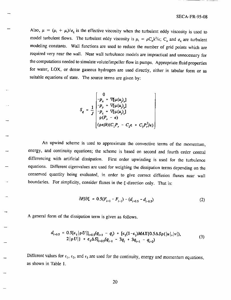
suitable equations of state. The source terms are given by:
0
-I,+
p(p,-
-c: +
An upwind scheme is used to approximate the convective terms of the momentum,
energy, and continuity equations; the scheme is based on second and fourth order central
differencing with artificial dissipation. First order upwinding is used for the turbulence
equations. Different eigenvalues are used for weighing the dissipation terms depending on the
conserved quantity being evaluated, in order to give correct diffusion fluxes near wall
boundaries. For simplicity, consider fluxes in the G-direction only. That is:
OF/O_ = 0.5(F_., - F__z) - (d_+o.5 - d__o.,) (2)
A general form of the dissipation term is given as follows.
d_+o.s = 0.5[_IpUl]_+o.s(q,+l- qg) + [%(I-_)MAXIO.SASPfluI, Iv[),
2[pU[} + eaAS]i+0.5(qi_ 1 - 3qi + 3qi.x - q/÷2)(3)
Different values for el, c2, and e3 are used for the continuity, energy and momentum equations,
as shown in Table 1.
20

SECA-FR-95-08
Table 1. DissipationParameters
Momentum& Energy Continuity
et dl 0
_2 0.015 0
e3 0 d 3
where: dl = REC and d3 = 0.005
To maintain time accuracy, a time-centered, time-marching scheme with a multiple pressure
corrector algorithm is employed. In general, a noniterative time-marching scheme was used for
time dependent flow computations; however, subiterations can be used if necessary. The
pressure corrector scheme is described as follows. A simplified momentum equation was
combined with the continuity equation to form a pressure correction equation. This equation is:
Opui/Ot --- - Vp'
or in discrete form:
ui' = - #(zxt/p)Vp' (4)
where/3 represents a pressure relaxation parameter (/3 = 10 is typical). The velocity field in
the continuity equation is then perturbed to form a correction equation. That is:
V(/OU'_ n+l = V[.On(Ui n + Ui')] = 0
or,
VCou?)= - VCoui)° (5)
Substituting equation (4) into (5), the following pressure correction equation is obtained.
21

w
SECA-FR-95-08
- V(flAt Vp') = - V(,ou._ _ (6)
Once the solution of equation (6) is obtained, the velocity field and the pressure field are updated
through equation (4) and the following relation.
p,,+l = p, + p,
To ensure that the updated velocity and pressure fields satisfy the continuity equation, the
pressure correction procedure is repeated several times (usually 4 times is sufficient) before
marching to the next time step. This constitutes a multi-corrector solution procedure.
The velocity through the impeller is calculated relative to the impeller, transformed to
a fixed coordinate system at the impeller exit, and passed to the volute as a boundary condition
along a zonal boundary. Since the grid points across the zonal boundary do not have a one-to-
one correspondence, a linear interpolation is used for the overlaid grid points. The interpolation
scheme along the zonal interface is applied implicitly inside the matrix solver to obtain better
convergence.
3.2 2-D Volute Simulation
A general unsteady impeller/diffuser interface boundary condition treatment was
developed and tested. The current model can be employed for steady-state or transient
computations; however, the transient simulation would be very computationally intensive. A 2-
D impeller/diffuser test case of Caltech, see Appendix A, was used to develop the computational
model. The Caltech impeller geometry includes a logarithmic spiral blade shape and several
diffuser vane profiles. For this study, a general cyclic boundary condition treatment was also
implemented, based on multi-zone zonal interface solution procedures. This allows the use of
patched cyclic boundaries without overlaid grids.
To establish a feasible procedure for optimizing the volute pressure distribution based on
CFD analysis, a generic 2-D volute test case was generated. A 2-zone volute model was
22

SECA-FR-95-08
formulatedwith theouterwall contouradjustablethrougha shapefunction. The objectiveof
this calculationwas to find a volute outer wall shapethat will minimize the net force on the
impeller.
For the 2-D volute test case, the side force optimizationalgorithm was tested. The
objectivefunction to be minimizedis the force on theimpeller andthe independentvariable is
the volute spiral angle. A relaxedversionof Newton's iteration methodanda methodusing
parabolic interpolationwere tested. The impeller was replacedby a boundarycondition of
constanttotalpressureupstreamof thediffuser. Figures 16-17showthepressurecontoursand
velocity vectors for the initial volute geometry. After every geometryperturbation, some
numberof iterationsare requiredfor a convergedsolution. For this test, theslopeof theforce
versusspiralanglewasevaluatedevery200time steps,andthegeometryupdated.Figures 18-
19 show the pressurecontoursand velocity vectors after 8000 time stepsusing Newton's
method. The iteration history of the force is given in Fig. 20. Due to the non-linearnature
of the system,Newton's methodproducessevereover-shootsand under-shootswhich leadsto
slowconvergencetowardsa minimumsideforcegeometry. Thesecondmethodusingparabolic
interpolationwasmorerobust. Figure 21comparestheiterationhistory for bothmethods.The
feasibility of the impeller/diffuser flowfield couplingsimulationwasestablished,but it wasnot
practical to continuethecalculationto optimizethe spiral angleby CFD simulationsalone.
Theunsteadyimpeller/diffuservaneinteractionsimulationwasinvestigatedfor thissame
2-D configuration. A relatively small time stepsizewasusedfor time accuracy. 5260 time
stepswere integratedfor one impeller bladepassage.The extendedtwo-equationturbulence
modelwasemployedfor the turbulent flow computation. Pressurecontoursof the flowfield
solutionafter four bladepassagesareshownin Fig. 22. Thepressuretime historyon threevane
surfacesnear the leadingedgeareplotted in Fig. 23, for the last bladepassagecycle. It is
known that for this 5:9 bladeratio, thetrue periodicity is one completeimpeller revolution.
The computationwasextendedto eightbladepassagecycles. Pressurecontoursof the
23

- SECA-FR-95-08
Fig. 16 Pressure Contours of the I_id_1Volute Geometry
/'7
Fig. 17 Velocity Vectors of the Initial Volute Geometry
24

-- SECA-FR-95-08
\
)_'I!N=-! _"_E'_!X_AX= 2 =_E_'OI_IN=- 1 91E_IYMAX= I F_E_'01
A 6 3 L._3E_3G 7Q£_Z_3
c 7 I@23E_3
• 7 _87E4-03+" 8 2820E_-09@ 8 G7__E-_.3
i 9 4GI,TE-_j 8.8_.8E4-03
1 1 _C_'IE-_ a,m I. i_ 4E-,04.n 1 1_27E_o i. 1__ 1E-,04
r I.3_+04s i. ":13_.E+04
i.3787E+{_¢u 1._,!8_:E44_4
Fig. 18 Pressure Contours of the Optimized Volute After 8000 Time Steps
//
i
\
Fig. 19
/
/
II
Velocity Vectors of the Optimized Volute After 8000 Time Steps
25

SECA-FR-95-08
G ooe(Z-_o2
¢ 00(_E+02
2.000E+0_
_orce$
-2.0_E_02
-_-. 000E+02
_ Y-Fc_ceX-Fc-_ce
I '-G. 00_E+OZ0.0£+00 Z. 0£+03 4-._(Z+03 G. _Z+O_ 8. _(Z+_ 1._.l_.
Iterat ion
Fig. 20 Time Step History of the Force Using Newton's Method, Relaxed
G 8oo£+_2
Fig. 21
¢ _ .-+-op
F'or_s
2. _Z+02
0,00_E+000.0E+00
_ Method i Newton's method,
Method 2
relaxed
_-._using parabolic interpolation
I I t
2.01E+_ 4.. _4-03 G. _3
Iterat ion
Comparison of the Time Step History of the Force forAlgorithms Tested
the Optimization
26

-- SECA-FR-95-08
Inll -I glattoot
#_M• a 6swiIoel
Tnlm "1 ,e,e¢ eL
ovm_l L elel¢ eL
• ml| • IIIl¢oel
#m•• • Teelc.-e_
cog TOVm _Cv_S
IL_ll¢-ell
• 19Lt¢oo¢4oo_-ea
• _ Teat¢-e&
• rOJ1l-eat 11I¢_4 l
I 4,t 11_I--1 _
l • t IIBIIIII
TZl t¢ ol
6.TTllC-ea
F, • T_I$¢*o&
• * t.lt¢-e&
• *, 748B¢°0_
4.75.1E-cA• 5e_¢ ez4. -
m 4._0411-oI
u _._'IOtI-eZ
Fig. 22 Pressure Contours of the Impeller/Volute Test Case
Fig. 23
t ¢ _.er.e_ ,
I IOI I * IZ
PRESS
I . 1@3 T .e_. --
1.eol£-ez --
i. II.-_-_,mQ
........ $ t h-'..xs._.o
/'%
./" \
./
\"\ ,I
/
%, /"
I. eeel_oO_. I
el o(* eo l.olic * el I . qlc * ol
TZI_E
Z.O_ O&
Pressure Time History Near the Leading Edge of Selected Volute Vanes Over
One Blade Passage Cycle of the Impeller/Volute Test Case
27

SECA-FR-95-08
flowfield solutionareshownin Fig. 24. Figure 25 showsthe time history of thepressureon
the leadingedgesof threediffuser vanesover the lastsix bladepassagecycles. The effect of
the initial guessis still evident in thepressurehistory. More computationcyclesare required
to wash-outthelow frequencydisturbances.The unsteadysimulationis feasible,but thenumber
of impeller cyclesrequiredto obtaina quasi-steadyflow is excessive.
3.3 3-D CFD Simulation of Volute A
The flowfield for Volute A, shown in Fig. 4, was simulated for two representations of
the flow from Impeller X, shown in Fig. 5. The first simulation was for boundary conditions
upstream of the impeller and yielded a fully coupled CFD impeller flowfield prediction. The
coupling consisted of interpolating the impeller exit conditions to serve as the volute inlet
conditions across the zonal interface as described in section 3.1. The second simulation
consisted of using the Adkins/Brennen impeller model and interface matching parameter, B, to
approximate the impeller/volute coupling. The results of these predictions are given in the
following two subsections.
3.3.1 CFD Simulation of Both Volute A and Impeller X
To utilize an inlet boundary upstream of the impeller, grids for the impeller and the
volute were generated, and the coupled impeller/volute flow was calculated. The impeller grid
and the volute grid are shown in Figs. 26 and 27, respectively.
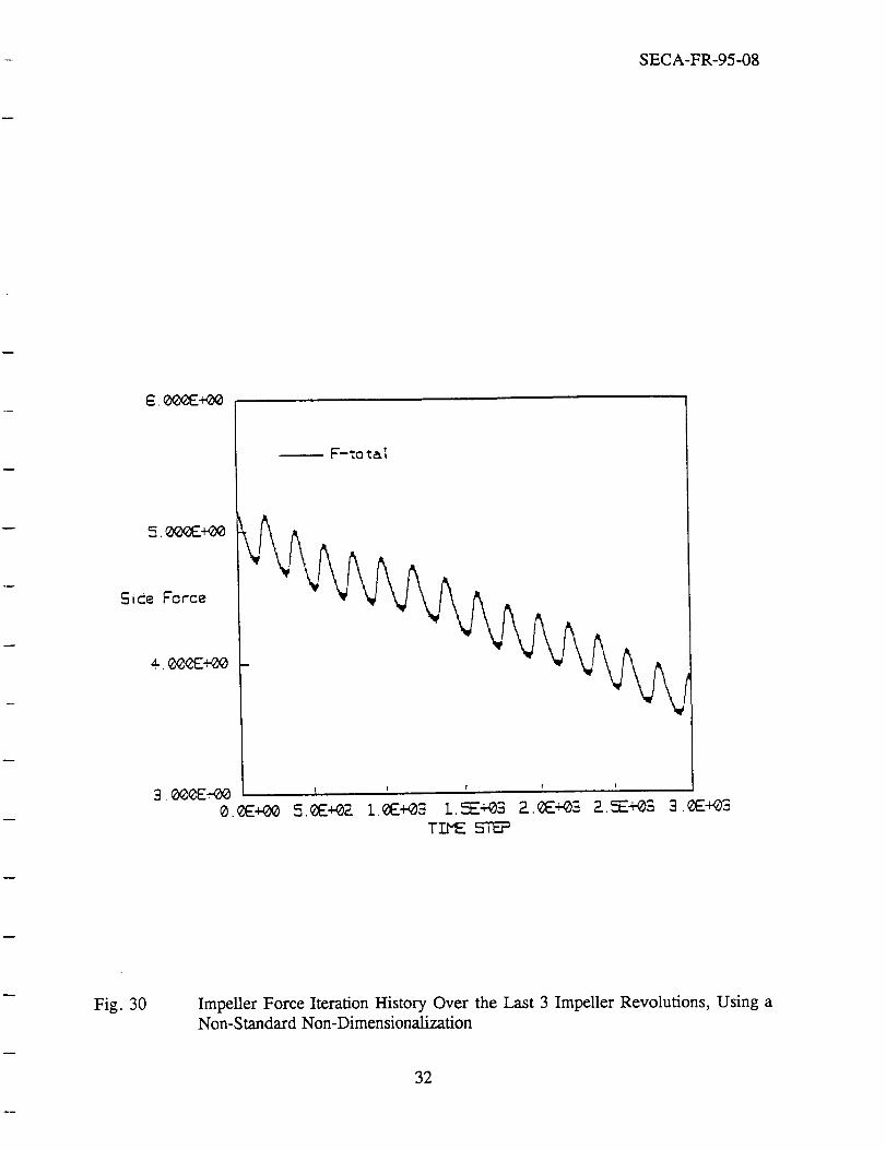
The flowfield computation was simulated for the design flow coefficient of so=.092.
Figures 28 and 29 show the pressure contours and velocity vectors after 6 impeller revolutions.
The solution is not yet periodic, indicated by the impeller force iteration history shown in Fig.
30 for the last 3 impeller revolutions (3000 iterations).
The volute discharge exit was extended further downstream to enclose the recirculation
region that had been observed in the design flow coefficient, so=.092, computation, and the
computation continued. Figures 31 and 32 show the pressure contours and velocity vectors.
28

SECA-FR-95-08
S;:_TA OATA(VLUTI:'I) _ C:_lTO.f:_
rain -I "mn_r_l
5 24,41,_8
Fig. 24 Pressure Contours of the ImpeUer/Volute Test Case After Eight Blade PassageCycles
Fig. 25
1 50OE*Oe
OGGE÷OQ
2*CP
5 eOeE-01"
00,O_E_@e
POINT I
I_ ..... POINT Z
pOINT 3
.%
/ ./\
t. /._, ._./ ,Li" _ ,'_ ._. .j "._ /,
.1"_../ ,"" ,-, "_-,,./" _.
I I I I I I I I I20 40 6O
TIHE
Pressure Time History Near the Leading Edge of Selected Volute Vanes Over Six
Blade Passage Cycles of the Impeller/Volute Test Case
29

SECA-FR-95-08
Fig. 26 Impeller, Without Shroud,ShowingTwo Blades
Fig. 27 Volute Grid
30

SECA-FR-95-08
/ i
(lFig. 28 Pressure Contours
)¢_IN=-7 5_E_-00XI_X= 8 _E_
C_ Ior-t_a 9 ?_74_E_ lb 9 4013E_4_Ic 9 5P-SaE_ id 9 G555E_ I• g 7_',-0 £? 9. $0_7E_1g t. _36E4__h 1 .O 163E_e_i 1. _.91E+02
1 1 067?_.E4__m 1.07e_E+_-n t O=r_r_r_r_r_r_r_r_r_*__o £.I_E3E_-O_
q l. 1307E+_-r l. !4-3=Fq'_-S 1. _+O2.t 1 16_E-_02.
Fig. 29 Velocity Vectors
)_IN=-7 i_-_>_AX= 9 ®1E-_OYMIN=-5 _+_I_AX= 8 _2E_
Co lor-Mexo
b 2 7L_-SE-O ic 5 _IE-O id 8 3_3E-01e i !17E+_¢ i. 3£72E+eO
i E_7_7E_h i _ IE-_i _. ES5E+_Oj Z.5151E+00
m 3 3_ _E+_0n 3 _32_+_c 3 9 ;2_3E+O0
9 4-4-7 _E+00r ¢. 7507E+00
5. 0302.E+00
u 5 5E_IE+O0
31
SECA-FR-95-08
6. _+@0
Side Force
F-'_o'cal
1
I I I I
T.T.P_ STEP
Fig. 30 Impeller Force Iteration History Over the Last 3 Impeller Revolutions, Using aNon-Standard Non-Dimensionalization
32

SECA-FR-95-08
Fig. 31
XMIN=- i.E_TE-_1)_tAX= i.ETE+O iYMIN=-5. IEE+00'rMAX= P_._+01
Co 1or-M_X=:a 9.734_E+01b 9.85E_E_Ic 9._3E+01d i.010CjE+O_-e i.0___33E+_¢ 1.035EE+0_S 1. _,B3E-__h 1_._:_7E-t-02i i. 0732E+02
j 1. I_7E.._2k I.09E__E+O_I I.IIOEE44_2m i.12_3IE+0Zn i.I__5EE+02o i.14_ IE+02p I._-_29 1. 173_E-_2r i. II_+02s i. L_975E+0Zt 1.21(_4E+02u 1.Z22_qZ+_-
Pressure Contours ¢ = .092
f/l , /,J . -- -- . _ -- - _ _ k_\\_ \ _', ,
/ " ,", _" " , I / -""_- "-X_.k / .... "1.,'//_ . "d; ; , I < "...".--_-7--_:-T_-_'--.,_\v,<\f ..... ,,I
• 1 /" _ _ _' # " "" .... t _#,
" I I ill x __ ' "1; Ill. _ ' ' '_
\_ ,,k _.. -_ _..:..i, l,' 'fn. ,,/\ ._'\\ "----'"5", / / _.', 7
\\_ x x .. . i
.,, ,.
Fig. 32 Velocity Vectors ¢ = .092
)@IIN=-J5E)EE+00X_AX= 7 0_-E_,_0
"fMIN=-5 IEE+00YMAX: 5.8SE_-00
Co Ior-l_
b 2. 9 IE_E--OIc 5 E_G7E-O id 8 755 IE"O Ie 1. :1673E-_0
g i.75 I_E*¢0h 2 G_ZEE+00i 2_._3_7E+_0
j 2. t___-_-_2. _IB3E+_
1 3 2-10_E+00m 3. _02_E'_'00
n 3.7E_EE+_
p ¢ 377_+00
r 49G12E+O@s 5.2..53E*eO
u 5 E_G7E+00
33

SECA-FR-95-08
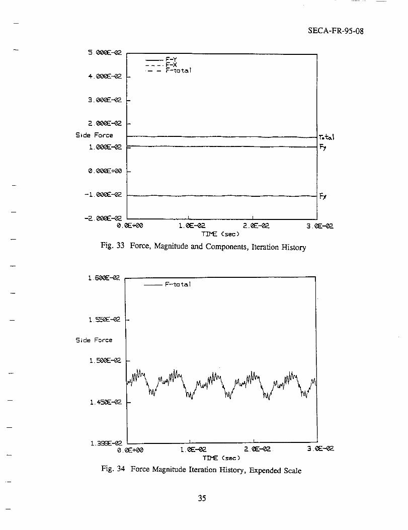
The impeller force is calculated by integrating the pressure at the impeller exit. The force
iteration history is shown in Figs. 33 and 34 for the last impeller revolution. Figure 33 shows
the force magnitude and its components, Fx and Fy. The origin is at the volute center with the
x-axis tangent to the tongue. Figure 34 is a plot of the magnitude of the force on an expanded
scale, showing the fluctuation from the impeller blades passing the volute tongue. Figures 33
and 34 also indicate that a fully-coupled 3-D impeller/volute flowfield solution was obtained.
The calculations were repeated for a range of flow coefficients. The time averaged
p(0) -P,.ut..circumferential pressure profile, cp(0)-- 2
.5 pu 2, on the shroud and hub sides (front and back,
respectively) of the volute at a radius ratio of r/r_pe_er exit = 1.08 is shown in Fig. 35 for
_b=.092. The kink in p(0) near 0=15 ° was believed to be grid dependent. The transition
between the fine grid near the tongue and the coarser grid around the spiral starting at 0= 15 °
was later modified. The calculated force components are shown in Fig. 36 with experimental
values from Adkins and Brennen (1988). The experimental values were obtained by averaging
the force measured by a rotating balance with the impeller placed at four positions 90 ° apart
along a circular whirl orbit. The calculated Fx does not resemble the experimental values. If
the kink in p(0) is flattened, the calculated force was expected to be closer to the measured
force.
Since the kink in the pressure profile mentioned was near 0= 15 °, where the transition
between the fine grid near the tongue and the coarser grid around the spiral occurs, the transition
was improved. The volute drawing was reviewed and some changes made to the grid.
However, obtaining fully coupled solutions requires large amounts of computation time,
therefore an alternate computation scheme was used to continue the investigation.
34
L
SECA-FR-95-08
5.00eE--_
¢ 0_E--02
2_E_2
Side Force
1_--02
g _xE+00
-1 _-02
-2. _l--O2O.gE
Fig. 33
--F-Y.... F-X..... F-total
1 I
1. _E--02 2. _i--02TII'_ (sec)
T°_!
F_
3. E--02
Force, Magnitude and Components, Iteration History
Side Force
i.5_E-_2
i.¢._E-g2
-- F-to t_l
i. 3SSE-02 _ i
g. _+@0 I. (E-02 2. E-02.
TIME (sec)
Fig. 34 Force Magnitude Iteration I-Iistory, Expended Scale
9.0E--02
35

SECA-FR-95-08
1 _+O0
9. _E-01 -
8._0_E-01
c_, (O)
7. _--01
G.0_E-01
0, OE+_
Fig. 35
Fro n tJ_s.... 8,_:k Temps
I I T
S.(Z_Z+Oi i.EE+02 2.7E+02
Theta-Deg.
Pressure Profile in the Volute, ¢ = .092
3. _'+02
t.m
I,
c-
o13.
E0
U
0b-
k.
E
0.10
0.08
0.06
0.04
0.02
0.00
-0.02
-0.04
-0.06
rl
0
rl
o Fx Adkinsn Fy Adkinszx Fx c alculatedo Fy calculated
0 n
0
0
0
A
nO 0 0
_ o o
0
0
I , I i l , I = I , I = I , I
0.04 0.05 0.06 0.07 0.08 0.09 0.10 0.11
Flow Coeffic ient
Fig. 36 Force Components as a Function of Flow Coefficient
36

SECA-FR-95-08
3.3.2 CFD Simulation of Volute A using Adkins/Brennen's Model for Impeller X
To reduce computation time, the impeller grid was removed and Adkins/Brennen impeller
model was used to establish the inlet boundary condition for the volute flowfield. The
Adkins/Brennen impeller/volute pump model and the test data to which it has been compared
is summarized in Appendix A. Briefly, the model assumes that the flow within the impeller
follows a logarithmic spiral. Bernoulli's equation is integrated along this path. The
Adkins/Brennen impeller/volute model will iterate to the spiral flow angle, given the head rise
across the pump. The impeller model provides a relation between the pressure and relative
velocity magnitude at the impeller/volute boundary in terms of a circumferential perturbation
function,/5. Equation A-6 in Appendix A is the differential equation which defines/5. Using
the experimental head rise across the pump from Adkins (1986), the impeller/volute model was
used to calculate the spiral flow angle (7) needed to use the impeller model as a boundary
condition.
The results from calculations for three flow coefficients, qS/4_a,ign=0.8, 1.0, and 1.1 will
be presented, where q5=.074, .092, and .101, respectively. Figure 37 shows the exterior
surface of the volute grid with the circumferential location labeled on which the pressure profile
will be presented at a tap radius ratio of r,_p/r2 = 1.08. The circumferential pressure profile,
p(0)- p(0)
2 , on the shroud and hub sides (front and back, respectively) of the volute is shown.5 pU 2
in Fig. 38. Note that the offset is p(0=0) in this figure. The kink near 0=350 ° is where the
tap radius crosses the re-entrant flow boundary. The pressure,p(O) -Pa
2 ' measured by Adkins.5 pu 2
with the impeller placed on a circular whirl orbit of rorbdr2 = 0.016 at the position nearest the
volute tongue is in Fig. 39. No test data are available for a centered impeller. The calculated
force components are shown in Fig. 40 with experimental values from Adkins (1986). The
calculated pressure more closely matches the experiment than the fully coupled CFD solution
presented in the previous section, consequently the force components are also closer to the
37

-- SECA-FR-95-08
sure tap circle
Fig. 37 Volute Grid, With Pressure Tap Circle Indicated
2. OOOE--01
1.0o_-o 1
0.000E+00
-1. 000E-0 ].
L----- 80% Flow _=. 074
-- 100% Flow q_=. 092
-- IIO*Z _'1o,_ q_=. lOl
-2.0OOE-0 i0.0E+00 9.0E+O1 i. 8E+O2 2.7E+02
The ta-Deg.
Fig. 38 Volute PressureProfile,From Computation
38

SECA-FR-95-08
1.0
0.9
0.8
0.7
0.6
0.5
| I I I I I | I | I | | I I I | I ]_. ' 41_ I.IF'" "o
VoluteA Impeller X .0"" e
Impeller near Volute Tongue _ =0.04 ....-.'"*"'*'" _A .o.UO,_P"
II o..4,,. °"_
( t; = 0 ° ) .,..,"'"'"" 0.06 .,. Y"" °'''_'.*'.0.. • ..,..,.,. ,,...,,...v... A ..'_' v...
,_° . ,'g'°, .i 0 ,,Y r' °" i°' °r !, ,°
.." jr""" " ._"_.:
- ."'* ..'" _ 0.08 ._""' 1t411 . "'_ """¢ u..4," _." '_"" .X. ,..... _ .. "4........ _," "_" _..",...... ,*..._.." "'" A_.'.-._ __..- ...-" - ..qi* _". , ,:_.. ""* . .._...., "._:::,::_,,.I.::_;_ll..I...|...,...J" _ _ _"'a"v..L....o _ .._.• " _."g."u.._ a . ..P"'4"'_'"o...la • .... ,l'"@ . C", I_ . .l" a
.le .._ .'g. r'" ."@' "".... o . "'9"'.ill -.,J. u_., tip' ,8.'"
? _...... ." ._,... * ....._....-....... , ""1,...0....... l..+'" • :•y .,k.*.ld v.. U • '""k.. o • .g "• • . g %,q •
:'. .',," "i.,.. 0.11 d""'' • .... "6"" o...Q' ""
• .'_, •
° i,.. t" ..
Tap• • , • e Front s
o,o,,,, Back Taps°
• °
• II q..._• •I I I
0I I I I I l I I I I I I I
60 120 180 240 :500
Angle from the Tongue, 8' (degrees)
Fig. 39 Volute Pressure Profile, From Experiment (Adkins 1986)
I I I
360
I,
C
c0(3.
@
0i,
e_
E
0.10
0.08
0.06
0.04
0.02
0.00
-0.02
-0.04
-0.06
--e-- Fx Adkins
m... -...o... Fy Adkins""... ,_ Fx calculated
"a... 0 Fy calculated
"',_
__130
ix ""_'
0
"'*.°.
"0
I , I I I , I i I i I , I i I
0.04- 0.05 0.06 0.07 0.08 0.09 0.1 0 0.11
Flow Coefficient
Fig. 40 Force Components as a Function of Flow Coefficient
39

-- SECA-FR-95-08
measured values. For the design flow coefficient, _b=.092, Figs. 41-42 show the pressure
contours and velocity vectors. The relative velocity magnitude perturbation functions, 13(0,'y),
from Adkins/Brennen impeller model used to specify the inlet velocity to the volute are given
in Fig. 43. The functions obtained using both the Adkins/Brennen impeller and volute models
are shown in Fig. 44.
These results were judged sufficiently accurate to warrant a parametric investigation of
the effect of volute shape on radial forces. The spiral angle of the streamline relative to the
impeller blade, 3', will, in general, not be known. For a postulated impeller and volute design,
the fully coupled impeller/volute CFD solution should be used to provide 3' for the design point
of the pump. As mentioned previously, 3' should be determined from the head curve for the
pump, and it will be a function of the flow coefficient. However, it is a weak function of flow
coefficient and may be assumed constant for modest volute variations and over a range of flow
coefficients. For large variations in volute geometry, 3' should be re-evaluated with the coupled
CFD impeller/volute simulation at the design point (for each volute evaluated).
4O

SECA-FR-95-08
)_MIN:-5.E_95+00)@'tAX:7._.E+O0YMIN:-S3. l..qZ+_OYMAX= 5.6EIZ+00
C._ lor-M_ :•", -7 ._-_b -6.4-17=_i-+00c -5.74-4.-=J:'-_00d -5.07 I.._;-_0
+" --3.77..,_+_g "--3.0_...._-1-00h -2.37cFI:'+(_i - 1.7e6_i-+00J -I._34E-_0
1 9. _-01m 8._'-01n i. _-,_0a Z.33L_E+_
q 3. G77_'+00r 4. 350E_-_0s 5.02_.3_'-_et 5. _E+e0u G. 36_EE+eO
Fig. 41 Pressure Contours q5 = .092
\
\
r r !
,t t I 11
l! I I If
/ / /
//
,%
Fig. 42 Velocity Vectors 4) = .092
_MIN=-_ _TE+_
YMIN=-5. l_q_+_YMAX= 5. _-.-_
Co 1o r-M_p •a 0.00_E+_b 2. 147EE-01c 4.. EE57E-O 1d G. 4436E-01e 8. _ I._--01_" i. 073_E+00
1. P_.887E-_Oh 7..50.qSE-_i 1.7 I_E+00
j I £331E+e0x 2. I,_7_E+001 __.3_=-1..00
m 2.5774E'_0n 2.7E_.E'_eo 3.007eE+00p 9 221E+00q 3. _,36EE+_r 3.6514E+00s 3.8662E-_0
u 4.. 2.S_E+00
41

-- SECA-FR-95-08
Fig. 43
110%
100%
8O%
9. E+O 1 i.8E+0_ 2.7E+02 3. E+02
Theta-Oe9.
RelativeVelocityMagnitude PerturbationFunction, From Computation
_.020 -
1.010
1.000
0.990
0.980
Fig. 44
| ' ' I I l J I i I , J J t A t t , I . , I I l I L t I i t J e , I I I I
0 90 180 270 360
e
Relative Velocity Magnitude Perturbation Function, Using Adkins'
Impeller/Volute Model
42

w
SECA-FR-95-08
4.0 DESIGN OF A TEST VOLUTE
Even though a small number of parameters are required to specify the volute shape with
the volute grid code (the spiral shape and the angle of the trapezoidal cross-section are the major
parameters, with the filet radii and circular shape of the outside of the cross-section expected
to be of minor importance), a large number of parametric cases would be required to obtain an
optimum volute shape. Also, the primary focus of this study was to develop the design
methodology, not to actually design volutes. Therefore, a limited set of parametric cases were
analyzed, and an interesting, but not optimal, new volute was selected for testing to verify the
methodology.
The predicted pressure distributions indicate that a major source of the radial forces are
the pressure disturbances caused by the tongue. This suggests that the tongue geometry could
be modified to reduce the separation in the discharge duct or that the spiral shape opposite the
tongue could be distorted to balance the disturbance at the tongue. Of course, other strategies
could be used. The promising shapes indicated by the experimental data shown in Fig. 3 could
be investigated. Unfortunately, the specific volute geometries tested to produce Fig. 3 were not
reported; therefore, the entire reconfiguring of the volute would have to be re-done. Due to
the finite funding available for this study, the concept of reducing the tongue distortion and
balancing this effect with volute geometry changes opposite the tongue were the only
optimization factors considered.
4.1 Parametric Studies
Changes were made to the Volute A surface to investigate their effect upon the force on
the impeller. The four volute geometries evaluated are summarized in Table 2. Since these
geometries are quite similar to Volute A, the value of 3' was held constant. The flowfields for
four flow coefficients: _b=.074, .083, .092, and. 101 were calculated.
43

SECA-FR-95-08
Table2. Volute geometries
case label cross-section modified spiral contourinterpolationmethod tongue
1 baseline spline no spline
2 modified tongue spline yes spline
3 arch spiral 186_+10 f(O) yes Archimedian
flat .5 spiral
4 arch spiral 186+5 f(O) yes Archimedian
spiral
For the first two cases presented, the surface of the spiral region was interpolated
between the defined cross-sections using cubic splines. The defined cross-sections were obtained
from the drawing of a Volute A, which had been tested at Caltech. For the first case, flow
separation was observed on the discharge side of the tongue for all of the flow coefficients
calculated. Consequently, the tongue contour on the discharge side was modified for the second
case. For the above design flow coefficient, the flow separation was drastically reduced, and,
for the other flow coefficients, entirely eliminated The modified tongue was kept for the
subsequent cases. Since the same differences exist between the simulated and the measured
forces for Volute A, the simulated forces were used for these parametric comparisons.
For the last two cases the spiral surface was described using the volute cross-section
geometry previously presented, Fig. 6. The cubic spline which had described the spiral
midplane contour was replaced by two Archimedian spirals connected with a two-point spline
to smooth the transition. For the geometry labeled "arch spiral 186+10 flat .5" the spiral
contour was flattened opposite the tongue. The spiral contour is shown Fig. 45-46 using
Cartesian and polar coordinates, respectively. The cross-sectional area in the spiral region and
its derivative with respect to 0 are shown in Figs. 47-48. In Fig. 47, 0 starts at the tip of the
tongue; however, the tongue is not included in Fig. 48.
For each flow coefficient calculated, Fig. 49-52 shows the change in the circumferential
44

SECA-FR-95-08
-- baseline
arch spiral 186+10 flat .5
arch s_ira1186+5
"-.",_. X_ modift_l tongue
Fig. 45 Volute Midplane Contour
t-O(.J
CL
co
5.5
4.0
3.50
i,.all _/' .'''*'" • f e t't _'/r" ,'" p" ,*
..... I , , , , , 1 , , , , , I _ A , , , t , , , , , I , .... I
60 120 180 240 300 360
e
Fig. 46 Volute Spiral Contour
45

SECA-FR-95-08
¢'_
t..
¢:ZO
¢J
d_t,O
£U
"I
1.5
1.O
0.5
0.00
baseline .t. "_''"
......... arch spiral 186-4-10 flat .5 .,.
arch spiral 186:t: 5 ,.r""
' ' ' ' , I , J l , , I , , , j , I , , , I a I I i I I , | I ! t , I I
60 120 180 240 300 360
e
Fig. 47 Volute Cross-Section Area
0.0150
0.0125
0.0100
0.0075
0.0050
0.0025
0.0000
I baseline
::::::::: A_!
. . , , , I , , . I , , , , • I A , t , , I . , , A , I , , , t , 1
0 60 120 ! 80 240 300 360
e
Fig. 48 Slope of the Volute Cross-Section Area With Respect to 8
46

-- SECA-FR-95-08
2. oo8E-o I
I _--01
-1.0_E-01
-2 0_E--01O. 0£+00
Fig. 49
I --->-- S@_-C_o 1
C-_-C_o2_--,--- 8O_-Geo3
' I I
S._-_I i. 8E-_7_ 2.7E-_2
8, deg.
Volute Pressure Profile 4)/4_de,_-- •8
3.£E+_.
1 oee6--oI -
0. _+_
-i. O_E-Ol
-2. _)_E-O l0.0E+00
--e--- _-Geo 19_-Geo2_
--e--- _-Geo3
C-q_-C_c4
[ I I
$._+4_ 1 i._'+_- 2.7E+_.
8, deg.
Fig. 50 Volute Pressure Proffie, _/4)_. = .9
47

-- SECA-FR-95-08
2.00_IE-01 [i'i _-01
-I.0_E-01
-2. _i---010.0E+_
Fig. 51
---e---10@*_ 1
---e-- l_-Cec3
r ' I
S._+491 i._4"02 2.7E_'02
0, deg.
Volute Pressure Profile _b/_b_ - 1.0
2.ooe£-Ol
-I._-oi
-2. _--_ i0._
---9---llO_-Gec 11l_)_-C._c_
--e--- 1IO_-C_o3--->---II_-C_o4-
t P I
i'_0 9,_4_1 1._l+02 2.7E'+_.
O, deg.
Fig. 52 Volute Pressure Profile, _/4),m,_ = I.1
3._-_z
48

SECA-FR-95-08
pressure profile,p(O)- p(O)
, for the four geometric cases. For the last two cases with the
Archimedian spiral, the drop in pressure after the tongue was flattened. The calculated force
components are shown in Fig. 53, with the force magnitude in Fig. 54. Except for
_b/_bd,e,=l.1, the geometry changes tried shifted the Fx(0) and Fy(0) curves but did not
noticeably affect their slope. The tongue modification had the greatest effect on ff/_bd_,_n = 1.1.
The calculations shown in Fig. 54 were used to select the test volute design described in
the next section of this report. However, since the simulated radial forces indicated such a
strong dependence on volute geometry, another case was analyzed. The grid used for the case
labeled: "baseline: spline" for Volute A was observed to have an unrealistic convergence
immediately after the tongue. A new Volute A grid was constructed from the F{0} cross-
sections using piece-wise continuous circular arcs matched at the locations of the metal guides
in the form upon which the fiberglass shell was cast. The results of this case is shown as
"baseline: 3 point arc" in Fig. 55. The computed forces resulting from this geometry change
are obviously of the order as those caused by the other shape changes studied. The other
geometries studied did not exhibit the unrealistic convergence noted in the baseline case.
However, such sensitivity suggests that the carefully machined metal volutes would be more
susceptible to accurate CFD simulation.
4.2 Selection of the Test Volute
Although more parametric cases would have been valuable, the "arch spiral 186 + 10 flat
0.5" was chosen as the verification case. A somewhat wider broadened minimum region in the
force versus flow coefficient was indicated in Fig. 54, although the minimum was slightly higher
(when compared to Volute A). A design drawing of this volute is shown in Fig. 56. The volute
was manufactured and supplied to Caltech for testing.
The original plan was to manufacture the volute with fiberglass using a similar procedure
to that used to manufacture Volute A. However, subsequent investigation indicated that the test
volute could be made more accurately and for less cost by machining it from aluminum.
49

SECA-FR-95-08
i,
i,
o_e-_D
0
EO
O
Ok,,.
OI.a..%_
(1,)
(l.)o_
E
0.04
0.03
0.02
0.01
0.00
--0.01
--0.02I
0.07
Fig. 53
baselinemodified tonguearch spiral 186+1 0 flat .5arch spiral 1 864- 5
, I , I , I ,
0.08 0.09 0.1 0
Flow Coeffic ient
Force Components as a Function of Flow Coefficient
I
0.11
Q)"O
c-C7_O
ID
EOU_K-
(D
(Do_
E
0.04
0.03
0.02
0.01
0.00
.. zx baselineo. \", + modified tongue
x arch spiral 1 86+1 0 flat .5_,\ \'-,,
•.._,\\ ,, o arch spiral 186± 5
., .,,, \ -A,",, \ _ ",
x,..._\, /,'...i,""_X"x-._ /" .'2" .
_\"k, x//,, //k _. • °• • ,*"
I , I i I , I
0.07 0.08 0.09 0.1 0
Flow Coefficient
Fig. 54 Force Magnitude as a Function of Flow Coefficient
I
0.11
50

SECA-FR-95-08
1
O
d
uO
J
om
(.2
O u,-) O
e_.__c" oO oO 0
I1) Q _°_ _
q) c- e= _0o o o mC) L_ L_ c_
.1210121.121
<_O+
J
cL .+
\ \ x'.
k \ x'.
j J_ °o °°
J / o°
I "° °°°°
- / / ..iJ
_ °° °°
_.)_ ...4
" / / .."J • °°°
_z //-" ..."
J /..° **,*_"
/ / / /..."
/..6""z / j.
I , I t I
(N ,.--.O O O
c5 c5 c5
°
O
O
OOd
d
O o
(DO
C.D
OIJ_
00O
c5
O
O
.,<
O>...z:.,.._
° ,,..q
:3
O°,,-_
Or_
LT.,
epn_!u6ow e oJo-t .JelledUJI
51

SECA-FR-95-08
O
oi)t_
OE.)tl.l
O
tl.l t!ll'i
7--j _'i !
\
<I\ _ i'\/ I.! i!
111_1"..t: tit,,I _. ii_t II17
Q
t I _I
, _ I.i.!!i i,ll ._ t,ili tl_ i _i• 1t i1.1 • -_ _-.
t til .i ! I t _ ",!
b
t I
,!li 7'• i
._ .t t
t._J
#li!I
1¢l
i _,Ii ,
g
' ii
• I _,>
I
i1:i
i iL
t1- I
52

SECA-FR-95-08
O
t_
Or,.)
O>
,l
m' I
il-
*'] \f T
- I
>o
o>
|
-i--B
I
0
I!
I1||
I
53
SECA-FR-95-08
The use of a computer controlled milling machine was required to produce the volute. Such a
machining operation was accomplished by specifying the geometry in an IGES formatted file.
Obtaining an IGES file involves the transformation of the volute surface from one form
to another. The volute grid generator writes the grid out as a plot3d file, a set of discrete
points. The procedure used is to read the plot3d file, extract the surfaces, convert the discrete
point surface to a NURBS (Non-Uniform Rational B-Spline) surface, then write the NURBS
surface in an IGES file format. The discrete points in the plot3d file controls what the surface
in the IGES file actually describes. By obtaining an IGES file with a coarse grid, the created
NURBS surfaces can be compared with the intended volute through a fine grid. The grid
generator was brought to NASA/MSFC, where codes supplied by Mississippi State University
were used to provide the NURBS surfaces and the IGES files. These files were supplied to a
machinist and the test volute was fabricated.
54

-- SECA-FR-95-08
5.0 EXPERIMENTAL EVALUATION OF TEST VOLUTE
The test volute was evaluated in the Rotor Force Test Facility (RFTF) at Caltech. The
results of these tests are attached as Appendix B.
Figures 57 and 58 show a comparison of the measured and predicted radial forces on the
test volute. The accuracy of the simulation is quite good near the design point. At extremely
high and low flow coefficients, the trends are correct, but the accuracy is somewhat less.
Leakages and other factors not included in the analysis are probably the cause of the differences
observed. The CFD codes used for the design of the test volute are adequately verified by the
experimental measurements. The small geometric differences between the test volute and Volute
A indicate that the CFD analysis is sufficiently sensitive to evaluate design modifications.
Furthermore the verification suggest that good dimensional control must be exercised on
experimentally tested volutes to preclude obscuring important design features.
Figure 59 shows a comparison of the measured and predicted radial pressure distribution
around the test volute. The pressure coefficient is defined as:
= -
u2 is the impeller exit velocity. Pror in the FDNS simulation and in Appendix B are not the same.
This difference changes the magnitude of the pressure coefficient; therefore, the measured
pressure profiles were rescaled for comparison in Fig. 59. The obvious differences in pressure
for the two sides of the volute are due to the use of an assumed constant impeller exit velocity
from the hub to the shroud (which results from using the Adkins/Brennen impeller model) and
to leakage effects. The pressure profile fits are reasonable and apparently do not effect the good
force predictions shown in Figs. 57 and 58.
55

SECA-FR-95-08
I ' I ' I I I
o>
_ V
X X _,
u_u- u2,,or)
C3 CJQ 0ta_ C25t__ C3
II
t • III
!1/
//
//
//
//
//
//
I// •/
//
/
//
//
tl IIIII
II
/
//
//
/
I I i ! , I I I i ! i 1
F'-- t..C3 _ ,--. ,:--.- r'O t.?)0 0 0 0 0 0 0
d o d c_ o c_ dI I I
,4-I 'x-I sa oJo__-I1o!p0_
Ir.O
,5
Oq
c5
0
0
0
Ob0
d
CO0
0
0
0
cO0
0
uO0
0
c-(b
°i
q.)
,.@..,.,.
0
0i,
M
0>.
¢¢1
<,9,o
.t,-,
0
t-
O
t_
.__
56

-- SECA-FR-95-08
¢.£3O
O
i 1 ' 1 ' I ' l
..---, Q
_O_> "O
_, t,/3 ,. J
U) o c
u_C_< []
• D [] O_
0 0 0 0 0
0 0 0 CD 0
D
r'O
d
d
d
0
d
O_0
d
CO0
d
0
d
qD0
CD
0
oo0
0
@°_
0_
@0
0
©I,
0>.
¢
0
0
aoxoj lOgO/
57

SECA-FR-95-08
_O
v_
©o
©©
ZZ_
LLO0
It"I I
<: • 4I I
I I
I i t
(33 I_
0 0
o 0
/ 1+,'t
0 0 0 0 0
0 0 0 0 0I I
00
oi,-O
©
00
' 0
1400
c5I
o,,
c_II
0>
[..
°l,-q
oo_
°_I-i
° ,,-,I
d o ]Ua! O!;;aO 0 aunssaJ d
58

SECA-FR-95-08
6.0 CONCLUSIONS
The following conclusions are drawn from this investigation:
(1) The volute grid generator is useful for investigating volute configurations.
(2) Coupled impeller/volute CFD solutions are feasible, but they require excessive
computation time to provide parametric volute configuration studies.
(3) Using Adkins/Brennen's _-equation for impeller/volute coupling with a CFD volute
simulation provides an accurate and practical model for optimizing volute configurations.
The simulations are very sensitive to the volute geometry specified. The parameter 3' in
the Adkins/Brennen impeller model should be evaluated with at least one fully coupled
impeller/volute CFD simulation for each major impeller/volute configuration change
considered.
(4) The impeller/volute model described in (3) was verified by experimental measurements
for a single configuration. The agreement between the simulation and experiment is
excellent near the design flow coefficient, and becomes somewhat less accurate away
from the design point.
(5) The design methodology can be used to minimize, or set to a prescribed, value, the
radial forces on a pump by controlling volute geometry.
59

SECA-FR-95-08
7.0 RECOMMENDATIONS
To obtain the maximum benefit from this pump model code, the following
recommendations are offered:
(1) The grid generator should be extended to provide an option for creating volute surfaces
in an IGES format.
(2) The pump model should be used in its present form to parametrically study
impeller/volute interactions on radial forces over a wide range of volute configurations.
(3) The pump model should be extended to treat vaned volutes, vaned diffusers, and cross-
over ducts for multi-stage pumps. Parametric configuration studies should be made with
this model. Note that the effects of axial velocity gradients at the trailing edge of the
impeller vanes and of rotor/stator interaction are neglected in this pump model.
(4) The pump model should be extended to treat impeller/volute rotor dynamic interactions
by direct application of the Adkins/Brennen impeller whirl model to CFD volute
simulations. This extension should include applications to fluid bearings.
60

-- SECA-FR-95-08
REFERENCES
Ad_ns, D.R., (1986). "Analyses of Hydrodynamic Forces on Centrifugal Pump
Impellers," Ph.D. thesis, Division of Engineering and Applied Science,
California Institute of Technology, Pasadena, CA., 1986.
Adkins, D.R. and Brennen, C.E. (1988). "Analyses of Hydrodynamic Radial Forces on
Centrifugal Pump Impellers". ASME J. Fluids Eng., 110. No. 1, 20-28.
Agostinelli, A., Nobles, D. and Mockridge, C.R. (1960). "An Experimental
Investigation of Radial Thrust in Centrifugal Pumps". ASME J. Eng. forPower 82, 120-126.
Brennen, C.E., (1994). Hydrodynamics of Pumps, Concepts ETI, Inc., Norwich,Vt.
Chamieh, D.S. (1983). "Forces on a Whirling Centrifugal Pump - Impeller," Ph.D.
Thesis, Division of Engineering and Applied Science, California Institute
of California, Pasadena, CA.
Chen, Y.S., (1988). "3-D Stator-Rotor Interaction of the SSME," AIAA Paper 88-3095.
Chen, Y.S., (1989). "Compressible and Incompressible Flow Computations with a
Pressure Based Method," AIAA Paper 89-0286.
Chen, Y.S., (1993). FDNS A General Purpose CFD Code User's Guide, Version 3.0.
Jery, B., (1987). "Experimental Study of Unsteady Hydrodynamic Force Matrices on
Whirling Centrifugal Pump Impellers," Ph.D. thesis, Division of
Engineering and Applied Science, California Institute of Technology,Pasadena, CA.
61

- SECA-FR-95-08
APPENDIX A
THE ADKINS/BRENNEN PUMP MODEL
A.1 The Adkins/Brennen Impeller/Volute Interaction Model
To analytically describe the interaction of impeller/volute flows and forces, Adkins and
Brennen (1988) constructed a flow model for the impeller and for the volute which was matched
by iteration at the impeller exit and the volute inlet. This model accounts for whirl, but in this
investigation only impeller centered flows were considered. The impeller flow was modeled
with an unsteady form of the Bernoulli equation. This flow was assumed to be 2-dimensional,
and the whirl speed was assumed constant. The flow was also assumed to follow a spiral path
through the impeller at a fixed angle relative to the impeller. This angle was a function of the
flow rate and the head rise, as required to satisfy an experimentally determined pump curve.
Initial conditions for the impeller flow were no swirl and circumferentially constant total head.
The volute flow was described with a continuity equation, a moment of momentum equation,
and a radial momentum equation. The velocity profile in the volute was assumed to be flat
across a cross-section and vary circumferentially around the spiral. The resulting model
consisted of nine ordinary differential equations which were solved by iteration until pressure
and flow conditions at the interface between the impeller discharge and the volute inlet were
matched. Application of this flow model to the Volute A/Impeller X pump is shown in Fig. A-
1, from Adkins (1986). The model does not closely match the test data, but the proper trends
are predicted.
The Adkins and Brennen pump model was encoded from the listing in Adkins (1986)
dissertation for use as a stand-alone pump model and as a module to provide boundary conditions
for a CFD calculation the volute flow. The Adkins/Brennen impeller submodel describes the
flow between the inlet and discharge of the impeller with a simplified Bernoulli equation:
P/p+ 0.5(v 2 - f_2r"2) + j _. 3v ds" - ¢o2e j r cos{cot-fit-0"} dr"3t
- o_2e S _. sin{o_t-ftt-0"}r" d0" = F{t} (A-l)
62

-- SECA-FR-95-08
ILL
L_
u
m
(Dc"l
E1====4
c"-I,.--
c-O
03
c.)
OI1
0.16
0.12
0.08
0.04
0.00
-0.04
-0.08
. • | • • • •
Volute A Impeller X
.=ory
o o o ° o ° ° o ,
Xx
Y
Experimental-
"- Fx, Y-Fy
QI_-'
(1000 RPM, 4 Position average)
I i I _ a l . , 08 ' I I Io o.o2 o.o4 o.o6 o. oJo o._z
Flow Coefficient,
Fig. A-1 Radial forces on ImpeUer X in Volute A, theoretically calculated over a wide
range of flow coefficients, and compared to experimental measurements, fromAdkins (1986).
63

SECA-FR-95-08
The geometricvariablesusedaredefinedin Fig. A-2. The flow in the impeller is assumedto
follow a spiralpathwith inclinationangle3'which is fixed relativeto the impeller. For agiven
flowrate andheadrise, the spiralpath is describedby:
02" = 0" + tan 3' ln{r"/R2} (A-2)
The inclination angle is found by equating the theoretical and experimental head/flowrate
characteristics (_b_xp, in dimensionless form):
ff_p = 0.5[Dp{27r} + C_V2{2a'}]
where Dp is the volute pressure coefficient and V is the non-dimensionalized velocity in the
volute. Dp and V are evaluated with a centered impeller, and Cv is defined in terms of the
moments of the volute cross-sectional area.
To account for flow asymmetry, a circumferential perturbation, /3, is imposed on the
mean impeller flow, which is related to the relative velocity in the impeller, v, as follows.
v = [chflR22/r"]fl{O '', r",flt,o_t,e}sec{3"} (A-3)
For small eccentric whirl orbits, e,/3 may be linearized
/3{0",r",flt,o_t,e} =/30{02} + e'[fl_{02}cosoJt +fl,{02}sin_ot] (A-4)
64
SECA-FR-95-08
//y*I
II
S treamPath
\\
Impeller
X
\\
\
I |I Iii
ZVolute
Tonque
Fig. A-2. Geometry of a Centrifugal Pump Impeller, Adkins (1986).
65

SECA-FR-95-08
By combining equations 1, 3, and 4, and by assuming no inlet swirl and no circumferential total
pressure variation, the dimensionless inlet pressure may be written
P_'{R,,0,} = hi*-4,R/3o{02}[_bR/3o{02} + 2e'(o_/fl)sin{0,-o_t}]
- 2c'4_2R2_o{O2}[Bo{O2}coso_t + /3,{02}sino_t] (A-5)
By combining equations A-3, A-4, and A-5 and neglecting higher order terms,
Bernoulli's equation may be separated into harmonics with steady, c cos o:t, and e sin oJt
dependency. The steady term becomes
q5 sec23'[2 In{R} (d/3o/d02) + 4,/302] + Dp- 1 = 0 (A-6)
The sine and cosine harmonics will not be given here since they deal only with unsteady forces;
they are given in Adkins and Brennen (1988), hence/30 = /3.
The Adkins/Brennen impeller/volute interaction analysis was coded as a stand-alone code,
and Eq. A6 was used to provide inlet boundary conditions for flow into the volute. The
Adkins/Brennen analysis models the volute flow and solves the coupled set of equations for/3,
Dp, V, and 3' by iteration for a measured value of the head rise across the pump.
66

A.2 Caltech Pump Test Data
SECA-FR-95-08
Reports and records at Caltech were reviewed to obtain engineering drawings of the
Rotor Force Test Facility and of the various impeller/volute configurations which have been
studied. Most of the impeller-volute combinations were tested with Impeller X. Table A-1
describes these volutes. The circumferential increase of the cross-sectional area is shown in Fig.
A-3. The magnitude of the side force on Impeller X for these volutes is shown in Fig. A-4,
with the vaneless volutes in part (a) and the vaned diffusers in part (b). These measurements
were reported by lery (1987).
Two volutes were selected for modeling. The first one studied was a vaneless volute,
for which the grid generation was simpler. Volute A was selected since it was designed to
match Impeller X. Also, wall pressure measurements were taken at the volute inlet with the
impeller displaced from the volute center in four directions (stiffness measurement). Volute D
geometry was used as the basis of a 2-dimensional CFD simulation. No validation data exists
for Volute D other than total force measurements.
A listing of Adldns' pump model, WHIRL2, was obtained from Adldns (1986), but the
code was not available. The listed code was converted from Basic to Fortran and has been
checked against Adkins' published solutions. Drawings of ImpeUer X and Volute A used in the
comparison with Adkins' results were presented in Figs. 5 and 4, respectively. Software was
written to generate the volute cross-section integrals required as input by WHIRL2. The
integrals were calculated using the cross-sections in Fig. 4; however, the fillet radius at the
67

-- SECA-FR-95-08
Table A-1 VolutesTestedwith Impeller X at Caltech'sRotor ForceTest FacilityDatataken from Jery (1987)
VOLUTE
NAME
A
B
C
C
fD-O)
E
F
(D-6L)
G
fO-6S)
H
(DqeS)
VOLUTE
TYPE
VOLUTE
VOLUTE
VOLUTE
VANELESS
DIFFUSER
VANED
DIFFUSER
VANED
DIFFUSER
VANED
DIFFUSER
VANED
DIFFUSER
CROSS
SECTION
SHAPE
TRAPEZOIDAL
CIRCULAR
TRAPEZOIDAL
TRAPEZOIDAL
ELLIPTIC
TRAPEZOIDAL
TRAPEZOIDAL
SPIRAL
ANGLE
4
4
4
5
4
4
NUMBER
OF
VANES
0
0
0
0
17
TRAPEZOIDAL 4
6
LONG
6
SHORT
12
SHORT
VANE
ANGLE
18
10
15
15
68

SECA-FR-95-08
¢MIb
tn
<-ladI1¢,1¢
_1¢¢Z0I--
b.I03
I
0303
0n,-
u.II-
J0>
0
VOLUTE
120 24.0
DEGREES FROM TONGUE, 8
360
Fig. A-3 Volute Cross-Section Area for the Various Volutes Tested
from Jery (1987)
69

SECA-FR-95-08
0.20
¢)o%.,
0
" 0.15
"5
"6 0.10
_=
0.05
0.000.00
Fig. A-4a
IMPELLER X VOLUTE1000 RPM
o Aa B
\.\ " C. o D-O
I ] i
0.05 0.1 0,, Flow Coef
Magnitude of the Volute Force for Vaneless Volutes
0.15
0.20I i I
¢)(Jk_
O
" 0.15
O>
..(:
"- 0.100
"_ 0.05
0.000.00
Fig. A-4b
IMPELLER X VOLUTE1 000 RPM
o D-Oo En D-6La D-6S
_ D-12S
_'_..... I /" J I0 "
I .-A_- °.-°
.,_ o.°"
j. °°o-" _ •
" --., ° ..°--......... ............... -------- _ ""''"-.__"_- _,,--_- _ _..,--.---'_ _ _ q
0.05 0.1 0 0.1 5• , Flow Coef
Magnitude of the Volute Force for Vaned Diffusers
7O

- SECA-FR-95-08
volute inlet was ignored. Figs. A-5 through A-8 show plots providing a comparison between
the current calculations and results taken from Adkins (1986). The input integrals are given in
Figs. A-5 and A-6. These integrals were interpolated using quadratic and cubic splines for the
Adkins and SECA calculations, respectively. The model results can be compared by examining
the flow perturbation at the impeller discharge and the pressure distribution at the volute inlet
for several flow coefficients as shown in Figs. A-7 and A-8 for Adkins and SECA, respectively.
Notice that the Adkins/Brennen model predicts a static pressure discontinuity at the cutwater.
The conversion and implementation of the Adkins/Brennen code was successful.
The Adkins/Brennen code to model the impeller-volute flow for an impeller whirling on
a circular orbit within the volute was modified to eliminate interaction with the user during the
calculation of the steady, impeller centered, solution. Instead of the user comparing the
computed head rise with an experimental value, after having provided the impeller flow path
angle as input, the program will now search for the appropriate flow angle for a specified head
rise and tolerance.
71

0.4
0.3
0.2
0.1
0.0
• Volute A
• (Non-climensionalized using"'Impeller X geometry)
• • • ir_
SECA-FR-95-08
/f -o
/ -' .m
o/ ' / :-Io/// _" .o./ .l
": o_ _ o_ "_ _.0_ _ :.
• _ _ .,,,.,,0._, _ o-. _..._" _0 I 0..._ _ .¢B
L _ ,pi_"" I ......., .--. _... ,.....,- 0"" .
.,__._,)___L.- --- - InrA "al
• •
60 120 180 240 300 :560
Angle fromthe Tongue, 8 (degrees)
Fig. A-5 Moments of the Volute Cross Section, from Adkins (1986)
Eo
Volute A(non-d;mens;onol;zed us;ngIml_llfe_rX geomeb_)
rA
A
-rlnrA
inr A
6O 120 180 240
Angle from the Volute.Tongue, -J"
Fig. A-6 Calculated Moments of the Volute Cross Section
72

-- SECA-FR-95-08
_,_" 1.04 Volute A Impeller X
"°2 i,, /-__Z""--z-_-°'°8 ."4R
1.00 _0
o.98 i_- /_
o._ , ......... , iO 60 120 180 240 500 560
Angle from the Tongue, 82 (degrees)
Fig. A-7a Flow Perturbation at Impeller Discharge, from Adkins (1986)
O.
ir'_
41t-
.,=.
c-O
°_
r_°_v..
,m
41
¢/1It)
• 411
_i " ' i 14@ • w • • • • •
Volute A mpellerX
o#: _j! O.07 -o. f'
• • il • i i m • | • |
0 60 120 180 240 300 560
Angle from Volute Tongue, 8"(degrees)
Fig. A-7b Pressure Distribution at the Volute Lrdet, from Adl_s (t986)
73

SECA-FR-95-08
1.05
0r-
k.
1.00O
E0
._
0
1913_
0i,
0.95
i | i I
VoluteA Impeller Xi I i | i 1
=.06.07.08
.... .09
......... .10
0 60 1 20 180 24-0 .300 360Angle from the Volute Tongue, _2
Fig. A-8a Calculated Flow Perturbation at Impeller Discharge
Q,.C'n
..q=19
-3
O>
e"
O
c-O
om
.13o_
L
r'_
(,ool19k..
13._
1.0
0.9
0.8
0.7
0.6
0.5
a | i i t I i I i I J I
VoluteA ImpellerX
¢=.06.07.08
009
,\-_/_//5-- ...."" / P
N \ " - _'7 ..................... " ..... "
..... °
0 60 1 20 180 240 300 360Angle from the Volute Tongue, "d"
Calculated Pressure Distribution at the Volute InletFig. A-8b
74

SECA-FR-95-08
A.3 Instructions for UsingThe Adldns.for Code
A copy of the Adldns/Brennen code for the calculation of only the steady, impeller
centered, flow was provided to NASA/MSFC. An Input Instructions Guide is given below. The
I/O of the code was modified when it was implemented as a subroutine in the volute design
program.
Impeller/Volute Model Geometry
" .(r) )
!I!rv 2
.......
relative flow path.log spiral
cross-section integrals
X(o) - fri" w(r)dr
b2r2
i
rA (0) -f ri" rw( r) dr
lm'a(O) -
7_ (0) =b2r_
rlnr A(O) -
75

-- SECA-FR-95-08
Input fries of the volute integrals:
name.ext discrete data
0 i ,4(0 i) r-A(Oi) r'_(O) lnrA(e) rlnrA(Oi)
i.e. (O(O,(aregrl(i,k), k = 1,5), i = 1,n)
n = number of specified cross-sections
name.SPL cubic spline fit coefficients
((C1(i,k), C2(i,k), C3(i,k), C4(i,k), i=l,n-1), k=1,5)
where Spline(8) =
Cl(i,k) + C2(i,k) (0-0.3 + C3(i,k) (0-032 + C,(i,k) (0-033
0 in degrees, measured from the volute tongue in the direction of impeller rotation.
Program I/O
Impeller geometry: rl, 1"2,b2, w2 in code
Input:
Number of integration divisions, nd A0=27r/nd
Volute cross-section integral file (discrete data) 'name.ext'
program will read 'name.SPL' for cubic spline fit coefficients
Output file name
Query: store p(0'), B(Oz) for 0i i= 1,nd?
Flow coefficient,
76

SECA-FR-95-08
Find 3' (i)
or (2)
Enter the experimental head rise, search tolerance, and an initial
guess of 3'
Enter -1, flow path angle (3")
Query: is calculated head rise=experimental value?
If no, continue search, request another guess of 3'
If yes, proceed
output: (files appended)
output.MAT @ 3' _o Fo_ F_ nd
output.PBT @ 7 _'o Fo_ Foy nd
0'i Dpi /3i for i=l,nd+l
Nomenclature
b2
Dp(0')
Fo.,Foy
nd
P,,P,2
Pv
Q
h,r_
V_,VO
W2
(0z)
width of impeller discharge passage
pressure coef. at volute inlet = Pv(r2"O_)-Pa
.5 p(_r2 )2
components of the steady force on the
nondimensionalized by pvrb292r23
number of integration divisions
upstream, downstream total pressure
pressure at volute inlet
volume flow rate
impeller inlet, discharge radius
radial, azimuthal velocity relative to the impeller
external width of impeller discharge
impeller relative radial velocity perturbation
impeller in the volute frame,
77

SECA-FR-95-08
V¥
Ve
V r
,0r 13(02)r
tan y r I £ r < r 2
O'
02
P
impeller relative flow path angle
measured in stationary volute frame from tongue.
measured in translating (not rotating) impeller frame.
(for centered impeller, 0' = 02)
fluid density
flow coefficient = Q/(27rr22b2f_)
_0 total head coefficient Pa-Pa
p(_r2) 2
fl radian freq. of the impeller (shaft) rotation.
radian freq. of the circular whirl orbit.
The Fortran source code and sample input file of Adkins/Brennen model are stored in
the/u/te/garyc/volute/adkins directory, located at tyrell.msfc.nasa.gov.
78

SECA-FR-95-08
APPENDIX B
Radial Force Measurements
for the SECA Volute
Robert V. Uy
Christopher E. Brennen
Division of Engineering and Applied Science
Report No. E249.16, 1995
Report prepared for SECA, Inc., Huntsville, Alabamaunder contract with the California Institute of Technology.
B-1

Radial Force Measurements for the SECA
Robert V. Uy
Christopher E. Brennen
California Institute of TechnologyPasadena. Calif. 91125
volute
1 INTRODUCTION
This report contains the results of measurements of the steady radial forces on a centrifugal pump impeller
produced by a particular volute (the SECA Volute) designed by SECA. Inc. of Huntsville. Alabama. undercontract to the NASA George Marshall Space Flight Center. This SECA Volute was designed using CFD
methodology which SECA has developed to handle such flows. The purpose of the present tests was todetermine experimentally the steady radial forces by making measurements in the Rotor Force Test Facility
(RFTF) at the California Institute of Technology. This facility is described in detail elsewhere (Chamieh etal. 1985, Jery et al. 1985, Brennen et al. 1986, Adkins and Brennen 1988, Arndt and Franz 1986) and will
not be repeated here. For the purposes of the present tests, the fundamental components of the RFTF areas follows. A centrifugal impeller. Impeller X, is driven by an electric motor at speeds up to 2000rpm. The
impeller is mounted directly onto a rotating internal balance or dynamometer which measures the forces
imparted to it by the impeller. The forces are measured using strain gauges whose output signals emerge
through slip rings and are processed by a bank of instrumentation amplifiers. Since the forces sensed by thebalance are in a rotating frame, it is necessary to resolve them into forces in the laboratory frame. The time
averaged components of the radial forces are as defined in figure 1 where F_ is in the direction of the volute
cutwater and F_ is perpendicular to this. In section 3, we will briefly describe the impeller and various
volutes used in the present tests.The radial forces will be presented here in nondimensional form by dividing the forces by pTr122R3L,
where p is the fluid density, f_ is the rotational speed (in radians/sec), R is the discharge radius and L is the
width of the impeller discharge. The non-dimensional forces will be denoted by F_ and Fy. The magnitude
of the dimensionless radial force will be denoted by F0 = (F] + F2)¢, and its direction, 0, will be measured
from the tongue or cutwater of the volute in the direction of rotation.
2 R DIAL FORCES
The existence of radial forces, and attempts to evaluate them, date back to the 1930s (see Stepanoff's
comment in Biheller 1965) or earlier. The nonaxisymmetries which produce the radial forces depend upon
the geometry of the impeller and the volute as well as the flow coefficient, ¢. The latter is defined as Q/Af_R
where Q is the volume flow rate through the pump and A is the area of impeller discharge. Measurementsof radial forces have been made with a number of different impeller/volute combinations by Agostonelli et
ai. (1960), Iverson et al. (1960), Biheller (1965), Grabow (1964), Domm and Hergt (1970), Chamieh et al.
(1985), and Franz and Arndt (1986) among others.Some typical nondimensional radial forces obtained experimentally by Chamieh et al. (1985) for the
Impeller X/Volute A combination (see below) are shown in figure 2 for a range of speeds and flow coefficients.Note that the "design" objective that Volute A be well matched to Impeller X appears to be satisfied at a
flow coefficient, ¢, of 0.092 where the magnitude of the radial force appears to vanish.
The dependence of the radial forces on volute geometry is illustrated in figure 4 from Chamieh et al.
(1985) which presents a comparison of the magnitude of the force on Impeller X due to Volute A with the

Y Fo
X
Figure 1: Schematic showing the definition of the radial forces, r'_ and F,_, within tile volute geometry as
seen from the inlet to the pump.
0,.111_
0.14
0.11
0.I0
O.CI _"
O.OG
0.04
0.01
0u_
Fore Fey
IZ-.°• 0• Q
• d
-a.IC Ol_l
FlOW
oa_ V0
eQA _ V G _
SHAFT RPM I_
SO0
800tO00
I ZOOI ZOOZOO0
COEFFICIENT,
\%
' o.',- _,CLIO
Figure 2: Radial forces for the centrifugal Impeller X/Volute A combination as a function of shaft speed and
flow coefficient (Chamieh et al. 1985).

0.14
Figure 3: Comparison of the radial forces measured by Iverson, Rolling and Carlson (1960) on a pump with
a specific speed, No, of 0.36, by Agostinelli, Nobles and Mockeridge (1960), on a pump with No = 0.61, byDomm and Hergt (1970), and by Chamieh et al. (1985) on a pump with No = 0.57.
0.18
Q.I|
_ 0.14
<C o._o¢¢
r_ GO4o
17,1 O.04
i 0.0,1
C3.<:E o._
o
o
e4,
SHAFT RPM
Z_ 600
O. • 800
• _ 200
r VOUdrl"£ 8 _Q
_0 \(ClIIQJI,.J_ )0
,oAO_ o _o.eeoe o
A &o
o.io cLi2 0.14
FLOW COEFFICIENT,
Figure 4: Comparison of the magnitude of the radial force (F0) on Impeller X caused by Volute A and by
the circular Volute B with a circumferentially uniform area (Chamieh et al. 1985).

Figure5: Schematicof the impeller/volute arrangement in the RFTF used in the experiments of Chamieh
et al. (1985).
magnitude of the force due to a circular volute with a circumferentially uniform cross-sectional area. Intheory, Volute B could only be well-matched at zero flow rate; note that the results do exhibit a minimum
at shut-off. Figure 4 also illustrates one of the compromises that a designer may have to make. If the
objective were to minimize the radial force at a single flow rate, then a well-designed spiral volute would be
appropriate. On the other hand, if the objective were to minimize the force over a wide range of flow rates,
then a quite different design, perhaps even a constant area volute, might be more effective. Of course, a
comparison of the hydraulic performance would also have to be made in evaluating such design decisions.
In the past a number of different configurations of the "seal" at the impeller discharge/volute inlet were
employed during measurements of the Impeller X/Volute A radial forces. Specifically, figures 5.6 and 7 show
the different configurations employed by Chamieh et al. (1985), Adkins and Brennen (1988) and Franz etal. (1990), respectively (figure 8 shows the configuration employed in the current tests for both the Volute
A and the SECA Volute tests). Because the leakage flows in this region have an important effect on thepressure distributions acting on the impeller discharge and on the shroud, the radial forces differ somewhatfor each of these configurations. Further comment on these effects will be included later.
Visualizing the centrifugal pump impeller as a control volume, one can recognize three possible contri-
butions to the radial force. First, circumferential variation in the impeller discharge pressure (or volutepressure) will clearly result in a radial force acting on the impeller discharge area. A second contribution
could be caused by the leakage flow from the impeller discharge to the inlet between the impeller shroud
and the pump casing. Circumferential nonuniformity in the discharge pressure could cause circumferential
nonuniformity in the pressure within this shroud-casing gap, and therefore a radial force acting on the exterior
of the pump shroud. For convenience, we shall term this second contribution the leakage flow contribution.
Third, a circumferential nonuniformity in the flow rate out of the impeller would imply a force due to thenonuniformity in the momentum flux out of the impeller. This potential third contribution has not been
significant in any of the studies to date. Both the first two contributions appear to be important.
In order to investigate the origins of the radial forces, Adkins and Brennen (1988) (see also Brennen et
al. 1986) made measurements of the pressure distributions in the Volute A, and integrated these pressuresto evaluate the contribution of the discharge pressure to the radial force. Typical pressure distributions for

/
III
I
//
/
/ i ,/
Figure 6: Schematic of the impeller/volute arrangement in the RFTF used in the experiments of Adkins and
Brennen (1988).
I/f/i
I
Figure 7: Schematic of the impeller/volute arrangement in the RFTF used in the experiments of Franz ct
al. (1990).

7¸:
RADIAL GAP
rTIP LEAKAGE CLEARANCE --'------- _..
FRONT SEAL CLEARANCE, '/,_ iY
REAR SEAL CLEARANCE
Figure 8: Schematic of the impeller/volute arrangement in the RFTF used in the current tests.
O.9
0.8
O3
O.6
_ o.9
_- (3.8
8 o.T
= 0.6
meL
Volule A Lmoeller X .-
6 • O.07 i{
__1 I I I i i I I II I
P
/'*- Experimental:
_. * Front Tops
• Boci_ Taps
• 0.08
.I
O.9 " ¢-O.O9I
o.ep_. ./
0.7_"
0.6_. +,n.y_--. ..... i
0 60 t?.O 180 2.40 300 360
Anqie from the Tongue, e (degrees)
Figure 9: Circumferential pressure distributions in the impeller discharge for the Impeller X/Volute Acombination at three different flow rates. Also shown are the theoretica[ pressure distributions of Adkins
and Brennen (1988).

.p
t_
0 Io
o01
OOt,
Orn
0,00
,0.02
-O_t
-O.O6
,OCIIunt
, . , , . , , - ,
• _ Fovlo "._. ___ ?_oR_
O I'_ BALANCE MEASUREMEN'_
X + PRESSURE INTECRATION
, i . , . a , i
0.04 O_ O_ OW' 0 em 009 O.lO
FLOW COEFHCIENT,
Q
0|| 012
Figure 10: Comparison of radial forces from direct balance measurements, from integration of measured
pressures, and from theory for the hnpeller X/Volute A combination (from Adkins and Brennen 1988).
the Impeller X/Volute A combination (with the flow separation rings of figure 6 installed} are presented in
figure 9 for three different flow coefficients. Minor differences occur in the pressures measured in the front.sidewall of the volute at the impeller discharge (front taps) and those in the opposite wall (back taps). Ttle
experimental measurements in figure 10 are compared with theoretical predictions based on an analysis that
matches a guided impeller flow model with a one-dimensional treatment of the flow in the volute (Adkins andBrennen 1988), a theory which is similar in spirit to that proposed by Lorett and Gopalakrishnan (1983).
Integration of the experimental pressure distributions yielded radial forces in good agreement with boththe overall radial forces measured using the force balance and the theoretical predictions of the theory.
These results demonstrate that it is primarily the circumferential nonuniformity in the pressure at the
impeller discharge that generates the radial force. The theory clearly demonstrates that the momentum flux
contribution is negligible.The leakage flow from the impeller discharge, between the impeller shroud and the pump casing, and
back to the pump inlet does make a significant contribution to the radial force (Adkins and Brennen 1988,
Guinzburg et al. 1990}. Adkins and Brennen obtained data with and without the "flow separation rings"
of figure 6. The data of figures 9 and 10 were taken with these rings installed. The measurements showed
that, in the absence of the rings, the nonuniformity in the impeller discharge pressure caused significantnonuniformity in the pressure in the leakage annulus, and, therefore, a significant contribution from the
leakage flow to the radial force. This was not the case once the rings were installed, for the rings partiallyisolated the leakage annulus from the impeller discharge nonuniformity. However, a compensating mechanism
exists which causes the total radial force in the two cases to be more or less the same. The increased leakageflow without the rings tends to relieve some of the pressure nonuniformity in the impeller discharge, thus
reducing the contribution from the impeller discharge pressure distribution.
3 PUMP, IMPELLER AND VOLUTES
It is appropriate at this point to include a brief description of the pump components used in the present
tests.
Impeller X, which is shown in figure 11, is a five-bladed centrifugal pump impeller made by Byron Jackson
Pump Division of Borg Warner International Products. It has a discharge radius, /_ = 8.1 cm, a discharge
blade angle of 23 °, and a design specific speed, ND, of 0.57.In past studies frequent use was made of a volute designated Volute A (figure 12) which is a single exit,
spiral volute with a base circle of 18.3 cm and a spiral angle of 4 °. It is designed to match Impeller X at aflow coefficient of at = 0.092. This implies that the principles of fluid continuity and momentum have been
..--795--
4.37 1358
1
- J'ALL DIMENSIONSIN CENTIMETERS
Figure 11: A centrifugal pump impeller designated Impeller X.
PcQIQUfO0.1_J O. Prm Tin, Gircle
3.1q _
._..._'_
SU_m_ 8-e
Figure 12: A vaneless spiral volute (designated Volute A) designed to be matched to Impeller X.
utilized in the design, so that tile volute collects a circumferentially uniform discharge from the impeller and
channels it to the discharge line in such a way that the pressure in the volute is circumferentially uniform, and
in a way that minimizes the viscous losses in the deceleratin_ flow. For given volute and impeller geometries.
these objectives can only by met at one "design" flow coefficient. In the present tests measurements of the
forces on Volute A were included in order to provide a point of reference to the previous data base.
Also in the past. measurements were made (Chamieh et al. 1985) wilh a volute with a circumferentially
uniform area called Volute 13.
However, the purpose of the present tests was to obtain comparable data using SECA Volute. This volute
was fabricated elsewhere and shipped to Caltech. Some minor machining to the exterior was necessary iu
order to fit the SECA Volute into the RFTF but this had no effect upon the interior flow, The SECA Volute
was also provided with a circular array of pressure taps on the interior circumference, both on the front (or
flow inlet) surface and on the back (or drive shaft) surface. These were connected to banks of manometers in
order to measure the circumferential pressure distribution within the flow discharging from the impeller and
entering the volute. Similar measurements were carried out in the past on Volute A by Adkins and Brennen
(1988). In this report, we present not only measurements of the radial forces obtained using the internal
balance but also pressure distributions obtained using these pressure taps. The pressure distributions will
also be integrated to obtain values for the contributions to the overall radial forces due to nonuniformities
in the circumferential pressure distribution acting on the impeller discharge.
4 MEASUREMENT PROCEDURES
As in all past experiments. "dry" runs (experiments without water in the RFTF) were first conducted in
order to determine the tare forces registered by the internal balance. These tare forces were subtracted from
the "wet" runs to obtain the fluid forces imparted to the impeller by the flow. In addition the buoyancy
force acting on the submerged impeller was subtracted from the wet runs; this buoyancy force was obtained
by manually positioning the impeller in several different rotational orientations.
5 FORCE BALANCE DATA FOR VOLUTE A
The first set of measurements carried out during the current investigation consisted of further measurements
on the Impeller X/Volute A combination in order to provide a point of comparison for the later measurements
with the SECA Volute. Figure 13 presents the nondimensional forces in the x and y directions obtained at
a rotational speed of 2000rprn over a range of flow coefficients. This data is similar to, but not identical to,
previous measurements on the same combination obtained by Chamieh et al. (1985), Adkins and Brennen
(1988) and Franz et al. (1990). This previous data is compared with the current measurements in figures I4
and 15. The differences can be ascribed to the differences in the impeller discharge/volute inlet configuations
shown in figure 5 through 7. Specifically, the configuration used by Chamieh et al. (1985) (figure 5) is
substantially different from that used by Adkins and Brennen (1988) (figure 6) or Franz et al. (1990) (figure
7) since the absence of the flow separation rings reduces the pressure nonuniformity in the impeller discharge
but increases the pressure nonuniformity acting on the exterior of the shroud. The data of figures 14 and 15
reflect this configurational difference since the data from Adkins and Brennen (1988) and Franz et aL (1990)
is quite similar.
Some additional documentation on the current configuration should be recorded. Referring to figure 8
we note that
• The radial gap is a uniform 0.094in.
• The rear seal axial clearance is a uniform 0.004in.
• The tip leakage axial clearance is a uniform 0.007in.
• The front seal axial clearance was made as uniform as possible but still varied from 0.004in at top
dead center to 0.006in at bottom dead center.
10

©
©
<_=_
<
tq
<
©Z
0.04 •
002
000
-0.02
.-0.04
-0.06 *
0.04
B MII
0.06 0.08 0.10 0.12 0.14
m F•
• Fy"
FLOW COEFFICIENT, ¢
Figure 13: Current measurements of the radial forces for the Impeller X/Volute A combination obtained at
2000rprn.
0.10
O.OS
0.00
0-4).10
0.04 0.08 0.08 0.10 0.12 0.14
FLOW COEFFICIENT, ¢
Fx
Fy
o Fx. (C_mv_)
• F_ (Cemm_h)
o Fx (Fmnz)
A F_ (Fmz)
Figure 14: Comparison of the current measurements of the radial forces for the Impeller X/Volute A com-
bination with those obtained by Chamieh et al. (1985) and Franz et al. (1990).
11

010
©
<
<
L_
<
0Z
0.05
0.00
-0.05
a
-0.10
0.04 0.08 0.08 0.10 0.12 0.14
Fx
"---¢P'--- Fy
'_ F_, (Aclkins)
• Fy (Adldns)
FLOW COEFFICIENT, ¢
Figure 15: Comparison of the current measurements of the radial forces for the hnpeller X/Volute A com-
bination with those obtained by Adkins et al. (1988).
Note also from figure 8 that the current configuration differs somewhat from all three earlier configurations.It has greater similarity to Adkins and Brennen (1988) and Franz et al. (1990) than it does to Chamieh et
al. (1985) and the data of figures 14 and 15 show that the current forces display a similar relationship.
6 FORCE BALANCE DATA FOR THE SECA VOLUTE
The radial forces, F, and Fy, produced by the SECA Volute are presented in figure 16. Data was obtained
at both 2000rprn and at 1800rprn and it can be clearly seen from figure 15 that the non-dimensional datafor the two speeds is consistent. This has also been our past experience and indicates that Reynolds number
effects upon these results are minimal. Note that the magnitude of the force exhibits a minimum at a
flow coefficient of about 0.09 which seems to be the effective design flow coefficient for this impeller/volutecombination.
Also note by comparing figures 16 and 13 that the SECA Volute yields a small reduction in the magnitude
of the radial force when compared with Volute A. However they both yield very similar results.
7 PRESSURE DISTRIBUTIONS
The circular arrays of pressure taps located on the interior surface of the SECA Volute just inside the voluteinlet were connected to manometer banks and data on the pressure distributions were obtained at two speeds
(1800rpm and 2000rprn) and several flow coefficients. The pressures were converted to pressure coefficients
by normalizing with respect to the dynamic pressure corresponding to the impeller tip speed (the reference
pressure is inconsequential). These pressure coefficients were then plotted against position as represented bythe angle from the cutwater measured in the direction of impeller rotation. Similar plots were constructed
by Adkins and Brennen (1988); a sample was presented earlier in figure 9.
Five different pressure distributions for the SECA Volute are presented in figures 17 through 21, a series
with ascending flow coefficient. Several features of these pressure distributions are particularly noteworthy.
12
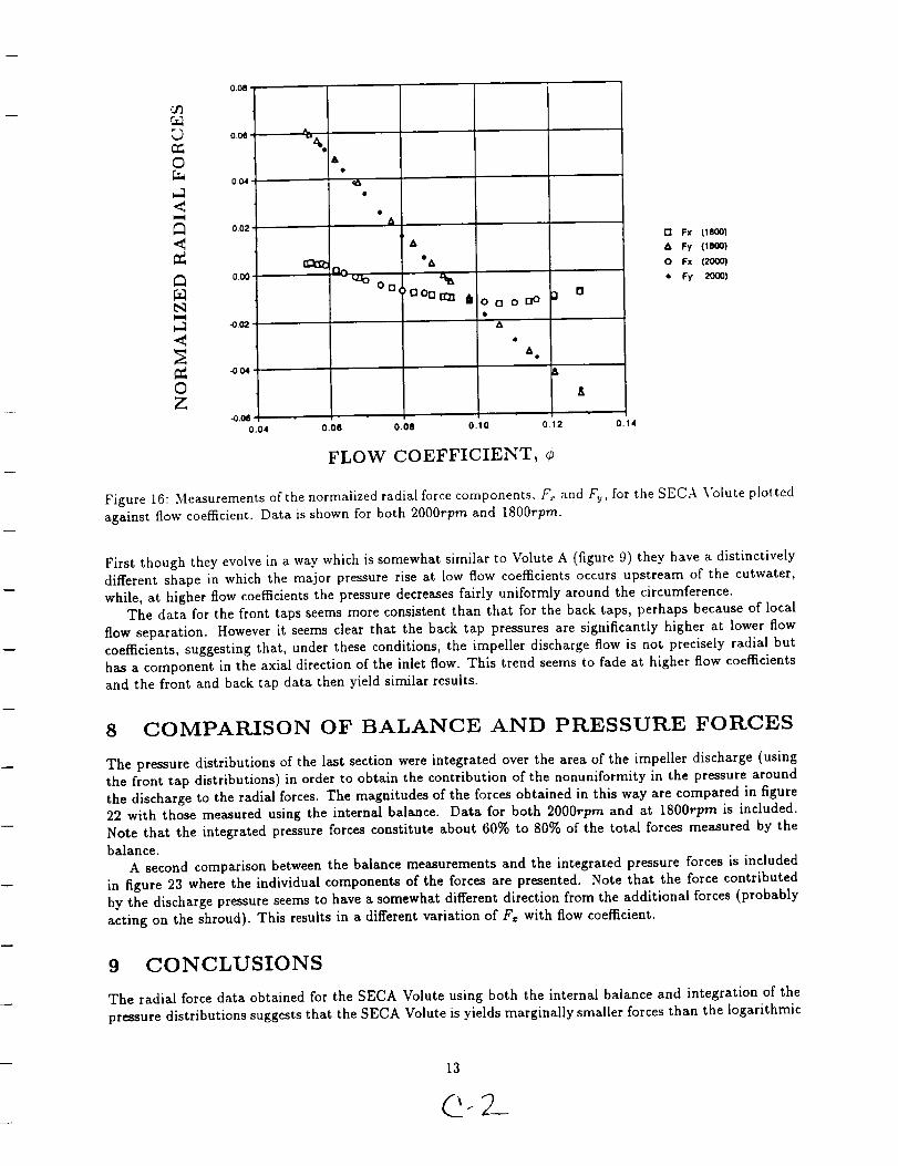
0.08 •
0.06'
©0.04¸
<
0.02
<
t_ -002
,<
-0.04
©Z
-0.0B
.04
,L
A
*A
a oo c_o iOo oD o
A o
0.06 _.08 ).10 0,12
FLOW COEFFICIENT,
0.14
r'l Fx (1000)
A Fy (1800)
O Fx (20(X)1
• Fy 2000)
Figure 16: Measurements of the normalized radial force components. F¢ and Fy, for the SECA Volute plotted
against flow coefficient. Data is shown for both 2000rpm and 1800rpm.
First though they evolve in a way which is somewhat similar to Volute A (figure 9) they have a distinctively
different shape in which the major pressure rise at low flow coefficients occurs upstream of the cutwater,
while, at higher flow coefficients the pressure decreases fairly uniformly around the circumference.The data for the front taps seems more consistent than that for the back taps, perhaps because of local
flow separation. However it seems clear that the back tap pressures are significantly higher at lower flow
coefficients, suggesting that, under these conditions, the impeller discharge flow is not precisely radial but
has a component in the axial direction of the inlet flow. This trend seems to fade at higher flow coefficientsand the front and back tap data then yield similar results.
8 COMPARISON OF BALANCE AND PRESSURE FORCES
The pressure distributions of the last section were integrated over the area of the impeller discharge (using
the front tap distributions) in order to obtain the contribution of the nonuniformity in the pressure around
the discharge to the radial forces. The magnitudes of the forces obtained in this way are compared in figure22 with those measured using the internal balance. Data for both 2000rpm and at 1800rprn is included.
Note that the integrated pressure forces constitute about 60% to 80% of the total forces measured by the
balance.A second comparison between the balance measurements and the integrated pressure forces is included
in figure 23 where the individual components of the forces are presented. Note that the force contributed
by the discharge pressure seems to have a somewhat different direction from the additional forces (probably
acting on the shroud). This results in a different variation of F_ with flow coefficient.
9 CONCLUSIONS
The radial force data obtained for the SECA Volute using both the internal balance and integration of the
pressure distributions suggests that the SECA Volute is yields marginally smaller forces than the logarithmic

1.10 "
Z1.05
0
0 loo
0
u']o.9s
m
il II mm
m •
I*
B e
0._ " "
0 100 200 300 400
ANGLE FROM CUTWATER
Figure 17: Pressure distributions for the SECA Volute operating at 1800rpm and a flow coefficient of 0.074.
1.10 •
Z:
ill
1.o6.
i-.,i
0
O.W
• •
• •
lOO
i 0 _l 0
20O
m _
elB
m_
• •
300 400
ANGLE FROM CUTWATER
Figure 18: Pressure distributions for the SECA Volute operating at 2000rpm and a flow coefficient of 0.079.
14

110 •
Z
! ,05'
©_,_ 1.00
c,n0.95
0,90
3Ii
B i •
I
me
De •
•U
100 200 300 400
ANGLE FROM CUTWATER
Figure 19: Pressure distributions for the SECA Volute operating at 1800rpm and a flow coefficient of 0.092.
1.10'
Z1.05
O 1.00
rj'j oJs
3
ill
OJO
0 100
k •
20O
• •lie,
m
Im
300 400
ANGLE FROM CUTWATER
Figure 20: Pressure distributions for the SECA Volute operating at 2000rpm and a flow coefficient of 0.098.
15

Z
1.10 '
1 05 '
©1.00'
u_0.95'
0.90'
41,1
)
100 200 300
ANGLE FROM CUTWATER
400
• Front raps
Figure 21: Pressure distributions for the SECA Volute operating at 1800rpm and a flow coefficient of 0.100.
0.04
0._
0.01
0
0.00
.01
|
0.011 0.09 O. 10 O. 11
FLOW COEFFICIENT, ¢
• Fo (2000) pmuum
• Fo('_O00) mlmce
• Fo(1800) prumme
• Fo(1800) bailance
Figure 22: Measurements of the magnitude, F0, of the radial force for the SECA Volute obtained at 2000rpm
and at 1800rpm. Both balance measurements and pressure integration measurements are shown.
16

0.03'
0.02'
©
<0.01 '
.<
o.oo.L'q),..4
.<
-0.01
0Z;
\\ a Fx I_1 (2000)
A "_'_ • Fx pmu 12000)
o FybW(2000)
• Fy press (2000)
• Fx hal (1800)
• Fx pmu (1800)
• Fy press 118001
-_:'.
0.07 0.08 0.00 0.10 0.11
FLOW COEFFICIENT, ¢
Figure 23: The components, F_ and Fy, of the radial force for the SECA Volute obtained at 2000rpm andat 1800rpm. Both balance measurements and pressure integration measurements are shown.
17

spiralVoluteA but tiledifferencesarenotlarze.
10 ACKNOWLEDGEMENTS
The authors are very grateful for the help provided by Joseph Sivo and by Christopher Hunter in conducting
the experimental measurements.
11 REFERENCES
Adkins. D.R. and Brennen. C.E. (1988). Analyses of hydrodynamic radial forces oll centrifugal pump
impellers. ASME J. Fluids Eng., 110. No. 1.20-28.
Agostinelli. A., Nobles, D. and Mockridge, C.R. (1960). An experimental investigation of radial thrust in
centrifugal pumps. ASME J. Eng. for Power. 82, 120-126.
Arndt. N. and Franz, R. (1986). Observations of hydrodynamic forces on several inducers including theSSME LPOTP. Calif. Inst. of Tech.. Div. Eng. and Appt. Sei.. Report No. E2$9.3.
Biheller. H.J. (1965). Radial force on the impeller of centrifugal pumps with volute, semi-volute and fully
concentric casings. ASME J. Eng. for Power. July 1965. 319-323.
Brennen. C.E.. Acosta. A.J., and Caughey, T.K. (1986). hnpeller fluid forces. Proc. .VASA AdvancedEarth-to-Orbit Propulsion Technology Conference. Huntswlle. AL. 2_MSA Conf. Publ. 2436, 270-295.
Chamieh. D.S., Acosta, A.J., Brennen, C.E., and Caughey, T.K. (1985). Experimental measurements of
hydrodynamic radial forces and stiffness matrices for a centrifugal pump-impeller. ASME J. Fluids
Eng., 107, No. 3,307-315.
Domm, H. and Hergt, P. (1970). Radial forces on impeller of volute casing pumps. In Flow Research on
Binding (ed: L.S. Dzung), Elsevier Publ. Co., 305-321.
Franz, R. and Arndt, N. (1986). Measurements of hydrodynamic forces on the impeller of the HPOTP of
the SSME. Calif. Inst. of Tech., Div. Eng. and Appl. Sci., Report No. E2,_9.
Franz, R., Acosta, A.J., Brennen, C.E., and Caughey, T.K. (1990). The rotordynamic forces on a centrifugal
pump impeller in the presence of cavitation. ASME J. Fluids Eng., 112,264-271.
Grabow, G. (1964). Radialdruck bei Kreiselpumpen. Pumpen und Verdichter, No. 2, 11-19.
Guinzburg, A., Brennen, C.E., Acosta, A.J., and Caughey, T.K. (1990). Measurements of the rotordynamic
shroud forces for centrifugal pumps. Proc. ASME Turbomachinery Forum, FED-96, 23-26.
Hergt, P. and Krieger, P. (1969-70). Radial forces in centrifugal pumps with guide vanes. Proc. Inst. Mech.Eng., 184, Part 3N, 101-107.
Iversen, H.W., Rolling, R.E., and Carlson, J.J. (1960). Volute pressure distribution, radial force on the
impeller and volute mixing losses of a radial flow centrifugal pump. ASME J. Eng. for Power, 82,136-144.
Jery, B., Acosta, A.J., Brennen, C.E., and Caughey, T.K. (1985). Forces on centrifugal pump impellers.
Proc. Second Int. Pump Symp., Houston, Texas, 21-32.
Lorett. J.A. and Gopalakrishnan, S. (1983). Interaction between impeller and volute of pumps at off-design
conditions. Proc. ASME Syrup. on Performance Characteristics of Hydraulic Turbines and Pumps,FED-6, 135-140.
18

SECA-FR-95-08
APPENDIX C
Operational Instructions for the
Volute Geometry Generation Code
C-1

-- SECA-FR-95-08
Discussion
The volute grid generation code that was developed as part of this contract is contained
on the UNIX tar tape VOLO1.TAP that is a part of the final documentation and deliverables.
The executable is named gdv and can be generated using the makefile - mkgdv. The input data
files required to execute the code are: Coordinate mapping file, geometry file, and a grid
stretching file. The input files contained on the tar tape that are used in this section to
demonstrate the operation of the code are: volnrn.dat, vol_bud.dat, volstr.dat, respectively.
Tables 1-3 list these three files for the sample case described in this Appendix.
The grid code is an interactive code that responds to user responses to queries by the
code. The operation of the code requires two cycles through the mapping portion of the code
which generates two files that describe the volute surface using a physical-surface coordinate
mapping natural to the spiral, discharge and tongue regions. The first mapping cycle generates
the mapping file that describes the surface of the volute except for the tongue region. The
output file for the first mapping is named by the user (in the sample case - vcp_bud.gi). This
file is subsequently used in the first grid generation cycle. The second mapping cycle defines
the tongue area surface. This cycle outputs a second user specified mapping file (sample case -
vcm_bud.gi), that is subsequently used in the second cycle through the grid generation module.
After the two mapping cycles are completed and control has returned to the top manu,
the user should exit the code since there is presently a "bug" in the code that does not allow
cycling through the grid portion until all the files are closed. The user can then re-execute the
code and proceed to perform the actual grid generation and preparation of the FDNS grid file.
The first cycle through the actual grid generation part of the code requires the user to
enter the first mapping file name (jcp_bud.gi). The code will also ask to enter a file name to
store the grid data. The user should enter a file name for this first cycle (vcp_bud.b) as this
output file can be used by the second cycle as an input file to avoid having to regenerate this
data during the second cycle. After the first cycle has been computed, the grid file generated
(vcp_bud.b) and control returned to the top menu, the user should select option b to specify the
name of the binary grid file (jcp_bud.b) in order to retrieve the previously generated grid data.
C-2

r
SECA-FR-95-08
Once this has been accomplished, the user then runs the grid generator a second time by
inputting the second mapped file name (vcm_bud.gi). Both cycles through the grid generation
have prompts for saving intermediate files for debug purposes. The user may or may not save
these files except for the second cycle where the user is asked: 'Store internal grid for
nreg=6?.' In this case, the user must respond with 'y' in order to generate the FDNS grid file.
The FDNS file is output to file vcm_bud.v6 for the sample case shown. The FDNS file will
always have as a first part of the file named the same as the first part of the second mapped file
name. The FDNS grid file is in the binary format type for FDNS.
Table A-4 lists all the prompts and responses that are required to generate an FDNS grid
for the sample case.
In order to simulate a volute flowfield, users need to run the grid generator,
/u/te/garye/volute/gridgen.ex located at tyrell.msfc.nasa.gov, to construct numerical grids.
The volute grid generator will create a file which contains the numerical grid coordinates. The
initial flowfield must be estimated directly by the user. Once the grid generation is completed,
rename (or link) the file which contains grid coordinates to fort.12, and rename (or link) the file
of initial flowfield to fort.13, which are the default Fortran units where the FDNS code reads
in the data of grid coordinates and flowfield. After the above steps are completed, users can
execute the FDNS flow solver,/u/te/garyc/volute/xfdns located at tyreU.msfc.nasa.gov. The
details of running the FDNS code are described in the FDNS user's guide (1993).
C-3

SECA-FR-95-08
Table A-1 Listing of Sample Problem Coordinate Mapping Input File - volnrn.dat
# nrng_region for grid and mapping generators# first character: #-comment
# s, t, d, nrspiral, tongue,discharge
# m,c nrmapping: theta,c
# n-quit
# s nrspiral
# 1,5,8,11,15,9,9,9,9,9
# 1,5,8,10,12,14,16,18,10,10
# 1,4,7,10,13,16,19,22,25,27
#j 1,3,0,4,7,8,9,11,10,10
#j 1,3,5,6,7,8,9,11,10,10 before inlet fillet
#s nr_spiral test inlet fillet, fillet conv
# 1,3,6,9,11,9,9,9,9,9
# 1,7,0,8,11,12,13,15,10,10
# 1,4,7,10,13,16,19,22,25,27
# spiral j should have j4-j2 > j8-j7
s nrspiral
1,3,6,9,11,9,9,9,9,9
1,3,0,7,8,0,9,10, 10,10
1,4,7,10,13,16,19,22,25,27
#mar 1,7, 0, 0,17,19, 0, 0,30,32
#j 1,3,0,7,8,0,9,11,10,10
#k 1,6, 0, 0,16,18, 0, 0,29,31
t nrtongue
1,3,6,9,11,9,9,9,9,9
1,3,3,7,9,10,10,10,10,10
1,3,6,9,11,10,10,10,10,10
d nr_discharge
1,3,6,9,11,9,9,9,9,9
1,3,6,9,11,10,10,10,10,10
1,2,2,5,7, 7, 9, 9, 9,17
#d nr_discharge ted: plot3d
# 1,3,6,9,11,9,9,9,9,9
# 1,3,6,9,11,10,10,10,10,10
# 1,5,5,10,21,21,24,24,24,27
# cheat in second mapping, replace d(10,3)= 17 with a smaller number
# to shorten straight pipeb nr blank
w
1,3,6,9,0, 11,9,9,9,9
1,2,2,2,0, 5,10,10,10,10
1,2,2,2,0, 7,10,10,10,10
#z nm_thetz theta_rv=nang
# 1,1,1,1,12, 10,10,10,10,10,10,10
# 1,9, 0,28,28,28,39,42,45,45,79,83
C-4
SECA-FR-95-08
Table A-1 Listing of Sample Problem Coordinate Mapping Input File - volnrn.datContinued
#
#
#
n
z2
# 1,2,1,10,11, 10,10,10,10,10,10,10
z nm_thetz theta_rv=nang ys 3-23-94
1,1,1,1,12, 10,10,10,10,10,10,10
1,6, 0,24,28,28,39,44,54,54,116,122
1,2,1,10,11, 10,10,10,10,10,10,10
#j recirc 1,17, 0,47,51,51,62,66,74,74,116,122
#j use 1,9, 0,24,28,28,39,44,54,54,116,122
#j 1,6, 0,24,28,28,39,44,54,54,116,122
#z nm_thetz theta_rv=nang ys 3-23-94, vol_caf shorten pipe1,1,1,1,12, 10,10,10,10,10,10,10
O, 1, O, 19,23,23,34,39,49,49,111,117
1,2,1,10,11, 10,10,10,10,10,10,10
va_yxsu before 4-22-94
1,9, 0,24,28,28,39,44,54,54,116,122
nm_thetz theta rv=nang
1,1,1,1,12, 10,10,10,10,10,10,10
1,9, 0,28,28,28,39,42,54,54,116,122
1,2,1,10,11, 10,10,10,10,10,10,10
c nm_c around tongue
1,1,1,1,10, 10,10,10,10,10
1,15,20,22,25,28,60,60,67,81
1,1,1,1,10, 10,10,10,10,10m nm thetb
1,5,7,7,13, 9,9,9,9,9
1,4,4,7,37,43,49,63, 10,10
1,1,1,1,10, 10,10,10,10,10n
d
cheat
nrdischarge
1,3,6,9,11,9,9,9,9,9
1,3,6,9,11,10,10,10,10,10
1,2,2,5,7, 7, 9, 9, 9,12
0,0,1,15,15,15,26,29,32,32,66,70nm thetz
1,1,1,1,12, 10,10,10,10,10
1,15,19,19,30,33,35,35,64,68
1,15,15,15,26,29,31,31,64,68
1,1,1,1,11, 10,10,10,10,10
C-5

SECA-FR-95-08
Table A-1 Listing of Sample Problem Coordinate Mapping Input File - volnrn.datContinued
m nm thetb
1,5,8,8,15, 9,9,9,9,9
1,4,4,7,37,44,51,65, 10,10
1,1,1,1,7, 10,10,10,10,10m nm thetb
1,8,11,21,21, 9,9,9,9,9
1,3,4,7,17,27,37,45, 10,10
1,1,1,1,10, 10,10,10,10,10#m nm theta
# 1,4,5,5,9, 9,9,9,9,9
# 1,3,4,7,17,25,27,34, 10,10
# 1,1,1,1,7, 10,10,10,I0,10
# 1,3,5,7,17,25,27,34, 10,10
c nm_c around tongue
1,1,5,5,9, 9,9,9,9,9
1,8,11,12,14,14,25,25,29,36
1,1,1,1,7, 10,10,10,10,10
n
C-6

SECA-FR-95-08
#v R2 B2 R3
# 3.1875 .62
#v R2 B2
# 3.1875 .62
v R1/R2 R2
.5 3.1875 .62
Table A-2 Listing of Sample Problem Geometry Input File - vol_bud.dat
#
# restart aw0
# baseline: spiral contour 3 pt arc NOT 1/8 inlet fillet
# rfc conv fixed with ishap91
# csectv(i,1)=hv use correct wr replaced .31 w/ .32# hv from drawing hv values wr fillet
# volute dwg rw=8.62 xv=5.8 rv(360)=5.79
# tongue from 3 point arc from drawing
# straight pipe extension 1 & m at housing chamber dwg coor, flange exitWR
3.3 .784
R3 WR
3.3 .784
B2 R3
3.3 .784 3.425 0 .125
# spiral cross-section control edges not use eccentricity yet,# use non-zero value, else kdschrg = 1 spline t0=0r
12
1 7. 1 1 1 1 1 -1 -1-1-1-1 40. 0.328
0 40. 0 0 0 0 3 0 0 0 091 40. 0.328
2 45. 4 0 4 4 0 0 -1-1 0 0 40. 0.52
0 50. 0 0 0 0 4 0 0 0 092 40. 0.520410. 0.
3 90. 7 7 7 7 7 0 3-1 051 40. 0.87
-.441070D + 00 0.140827D + 00 0.000000D + 00
4 135. 10 0 101010 0 -1-1 0 6 40. 1.18
44 1 0 0. 0. 0.
5 180. 13 13 13 13 13 51 3-1 051 40. 1.44
-. 360073D + 00 -. 199665D + 00 0.000000D + 00
6 225. 16 0161616 0 -1-1 0 6 40. 1.69
44 1 0 0. 0. 0.
7 270. 19 19 19 19 19 0 3-1 051 40. 1.89
0.150534D + 00 -. 293009D + 00 0.000000D + 00
8 315. 22 022 22 22 0 -1-1 0 6 40. 2.11
44 1 0 0. 0. 0.
9 360. 25 25 25 25 25 0 3-1 0-1 40. 2.49
0.130232D+00 0.489394D+00 0.000000D+00
10 367. 27 27 27 27 27 51 6 6 151 40. 2.5436 .2120744 34 0. 0. 5.
22 1 0 0. 0. 0.
# spiral surface splines along theta#
R4 DELRNG
3.425 0.
R4 IVLINRL RVLINRL
3.425 0 .125
WR R4 IVLINRL RVLINRL
0. 0..0625
0. 0..1875
.09004 0. .1875
.09004 0. .1875
.11114 0. .1875
.12984 0..25
.14551 0..25
.16059 0..3125
.17265 0. .3125
.18592 0. .375
.20883 0. .375
.1 .375
if use control, fix grvc nrnge(6,ned).le.kl spline spans entire region
C-7

SECA-FR-95-08
Table A-2 Listing of Sample Problem Geometry Input File - vol bud.dat
(Continued)
e
d2
e
e
fl
e
e
f2
e
e q=22
1 10
n
2
1 9 6 22 104 0 0.
9 10 6 42 103 4 5.
# t//c2//c3//c4
# c2 bc for rv(theta) spline at theta(1) n=nat bc s=specify spiral angle
# c3 tongue center, radius r=specify radius c=specify center
# fit arc between tongue and discharge edges f=fix radius e=fix endpt
# c4 tongue/discharge interface follow curve until tangent to discharge edge
# c=follow tongue circle s=circle and spiral spline = don't# before 3.72 .446 0. .12 0.0 .1875
tsrc tongue circle center (x,y,z), radius, spiral angle, rfi d3.7254 .451 0. .1246 87.27 .18"75
dl discharge exit: tongue wall
volute dwg rw = 8.62
1 5 0.244493D+01 0.826600D+01 0.000000D+00
discharge exit: casing wall
volute dwg rw = 8.62
1 4 0.580000D+01 0.637686D+01 0.000000D+00
housing dwg rw=8.625
1 5 0.575764D+01 0.860657D+01 0.000000D+00
flange exit: tongue wall
housing dwg
1 7 0.177287D+01 0.123214D+02 0.000000D+00
q =22
1 10 0.911767D+00 0.221638D+02 0.000000D+00
flange exit: casing wall
housing dwg
1 7 0.575764D+01 0.126700D +02 0.000000D+00
0.489655D +01 0.225124D +02 0.000000D +00
C-8

SECA-FR-95-08
Table A-3 Listing of Sample Problem Grid Stretching Input File - volstr.dat
# volute
# use '#' for to indicate comments
a use 'a' to indicate start of node distribution stretching parameters1 12 24 0.400000D+01 0.000000D+00
0 0 0 0.000000D+00 0.000(OOD+00
6 24 22 0._D+00 0.070000D+00
24 28 14 0.000000D+00 0.100000D+00
28 39 24 0.400000D+01 0.000000D+00
44 54 21 0.300000D+00 0.000000D+00
116 122 22 0.000000D+00 0.200000D+00
0 0 0 0.000000D+00 0.000000D+00
1 11 24 0.400000D+01 0.000000D+00
0 0 0 0.000000D+00 0.000000D+00
C-9

SECA-FR-95-08
Table C-4 Sample Execution of Volute Grid Generation Code
av310 [/usr2/ron/grid/opt] gdv
new gdv ........
c: create mapping
g: create cdr.id
b: reed existing grid data
n: execute options selected
r : reset program
q: qL_it program
select option c
Select mapping:
p: physical--surface coordinate
c : cross-section
a: Adkins' area integral defined spiral c-sections
b: Adkins' area integral along spiral region
d: discharge area integral
e: volute contour edge iges file
3: 3 point arc spiral contour
k: curvature of spiral c-sections
i: second volute mapping iges surfaces
t : psc .surface tongue reg'_on
m: Adkins' ffmpeller/vo]ute mode]
r: Adkins' model and restart flowfield file
z: mapping c zone: tongue')p
enter file for nrn data volnrn.dat
enter file for volute geo data vo]_bud.dat
enter idim (2-surface 3-volume) 2
et_ter file for mapping (don't write = ) vcp_bud.giselect option n
c: create mapping
b: read existing grid data
n : e.:',e¢'t2t,'.._ opt Ton:'; tel acted
r : reset program
q : quit r.)r'ogremselect option c
Se]ect mapping:
P=
C:
e:
b:d:e:
3:K :
t:
m:
r:
z:
:
physical--surface coordinate
cro_:s-sec t ion
Adkins' area integral defined spiral c-sections
Adkins' area integral along spiral reg_ofldischarge area integral
volute contour edge iges file
3 point arc spiral contour
curvature of spiral c-sections
second volute mapping iges surfaces
psc surface tong_Je re_'}on
Adkins' impeller/volute mode]
Adkins' model and restart flowfield file
mapping c zone: tonouG,'
C-10

- SECA-FR-95-08
Table C-4 Sample Execution of Volute Grid Generation Code (Continued)
enter node stretching file (none=) volstr.dat
enter idim (2-surtace 3--volume) 3
enter file for mapping (don't write= ) vcm_bud.gi
enter edge shape for interface 1-line, 3-arc, 8-log (center at tongue)
and (2) theta at r2,rv (deg) for interface between tongue and spiral regions8,360.,360.
add edges to pack grid near tongue
and to smooth re-entrant interface (if not line)
node distribution along spiral on r2
nr: 44 tongue 54 pack tongue 116 smooth 122 re-entrant
angle: 7.00 52.26 :_32.8!5 360.00 uniform dist
enter pack tongue and smooth angles (none=O,O) 30.,340.
add edges along r to adjust non-uniform arclength of spiral surface
in psc_surface interpolation, assume uniform spacingenter number of edges between that a 30.00 and
>0 will input there, <0 calculate equidistant
enter 4 intermediate (approx) angles (de{7)60,90,180,270
c: create mapping
g: create gr'id
b: read existing grid daten: execute options selected
r: reset program
q: quit program
select option q/
av310 [/usr2/ron/grid/opt] gdv
n_9_ odv ........
c create mappingg: create _:,id
b: read existing grid data
n: _;{_c_.{te options selectedr: reset programq: quit program
select option
select option q
enter mapping f '_.... ,¢,._ !,ud."T.,enter file to store grid data (don't= ) vcp bud.b
select optior_ n
Store edge coordinates for nre_- 2 ? {def=n) n
Store internal grid fc_ nreg= 2 ? (def=y) n
Store edge coordinates for n_g= 3 ? (def=n) nStore ffntern_ _ ,'jr_(_ _{_r ....... _- 3 ? (clef:y} n
store (r,the_a,z)? {de_r_ n
c: create mapping
g: create grid
b: read existing grid data
n: execute options selected
r: reset progr'am
q: quit program
b 340.00¢
C-ll

SECA-FR-95-08
Table C-4 Sample Execution of Volute Grid Generation Code (Continued)
select optio_ b
enter grid data file vcp_bud.b
select o_otior: n
c: create maprJing
g: create grid
b: read existing grid data
n: execute options selected
r : reset program
q: quit program
select out:io,P_ g
enter mapping file vcm bud.gi
select opt'_or_ n
Store edge coohdinates f_r nrea = 4 ? (def=n)
Store interne] a! _'+ _' .... _t;= _ _ /'.te_-:V_
Store edge coordinates re. _ .qreg = 5 ? (def=n)
Store internal grid for nreg= 6 ? (def:'y)store (r,theta,z)? (def=n)
c: create mapping
g: create Wl:'id
b: read existing grid data
n: execute options selected
r: reset program
q: quit program
select option q
ORIGINAL PAGE B
OF POORQUAI.n'Y
C-12