Seasonal variability of the equatorial undercurrent terminationand associated salinity maximum in the Gulf of Guinea

Nicolas Kolodziejczyk • Frederic Marin •

Bernard Bourles • Yves Gouriou • Henrick Berger

Received: 15 May 2013 / Accepted: 28 February 2014

� Springer-Verlag Berlin Heidelberg 2014

Abstract The termination of the Equatorial Undercurrent

(EUC) in the eastern equatorial Atlantic during boreal summer

and fall, and the fate of the associated saline water masses, are

analyzed from in situ hydrological and currents data collected

during 19 hydrographic cruises between 2000 and 2007,

complemented by observations from Argo profiling floats and

PIRATA moorings, and from a numerical simulation of the

Tropical Atlantic Ocean for the period 1993–2007. An intense

variability of the circulation and hydrological properties is

evidenced from observations in the upper thermocline

(24.5–26.2 isopycnal layer) between June and November.

During early boreal summer, saline water masses are trans-

ported eastward in the upper thermocline to the African coast

within the EUC, and recirculate westward on both sides of the

EUC. In mid-boreal summer, the EUC weakens in the upper

thermocline and the equatorial salinity maximum disappears

due to intense mixing with the surface waters during the

upwelling season. The extra-equatorial salinity maxima are

also partially eroded during the boreal summer, with a slight

poleward migration of the southern hemisphere maximum

until late boreal summer. The upper EUC reappears in Sep-

tember, feeding again the eastern equatorial Atlantic with

saline waters until boreal spring. During December–January,

numerical results suggest a second seasonal weakening of the

EUC in the Gulf of Guinea, with a partial erosion of the

associated equatorial salinity maximum.

1 Introduction

The Equatorial UnderCurrent (EUC) is the strongest zonal

flow in the tropical Atlantic Ocean, flowing eastward along

the equator within the thermocline. It is first the equatorial

branch of a large-scale meridional circulation—the Sub-

Tropical Cells (STCs)—that consists in the subduction of

saline and oxygen-enriched waters in the subtropics, and

their advection mainly within the southern thermocline to

the equatorial region, via western boundary currents and

interior ventilation (e.g., Blanke et al. 2002; Snowden and

Molinari 2003; Zhang et al. 2003; Hazeleger et al. 2003).

The EUC also contributes to the Atlantic Meridional

Overturning circulation (e.g., Lumpkin and Speer 2003;

Hazeleger and de Vries 2003; Hazeleger et al. 2003; Chang

et al. 2008). Most of EUC water masses then surface in the

This paper is a contribution to the special issue on tropical Atlantic

variability and coupled model climate biases that have been the focus

of the recently completed Tropical Atlantic Climate Experiment

(TACE), an international CLIVAR program (http://www.clivar.org/

organization/atlantic/tace). This special issue is coordinated by

William Johns, Peter Brandt, and Ping Chang, representatives of the

TACE Observations and TACE Modeling and Synthesis working

groups.

N. Kolodziejczyk (&)

Sorbonne Universites (UPMC, Univ Paris 06)-CNRS-IRD-

MNHN, LOCEAN Laboratory, 4, place Jussieu,

75252 Paris, France

e-mail: nicolas.kolodziejczyk@gmail.com

F. Marin � B. Bourles

Universite de Toulouse, UPS (OMP-PCA), Toulouse, France

F. Marin

IRD, LEGOS, Noumea, New Caledonia

B. Bourles

IRD, LEGOS, Plouzane, France

Y. Gouriou

IRD-US191, Plouzane, France

H. Berger

IFREMER, DYNECO-PYSED, Plouzane, France

123

Clim Dyn

DOI 10.1007/s00382-014-2107-7

central and eastern equatorial Atlantic (Hazeleger and de

Vries 2003; Rhein et al. 2010; Jouanno et al. 2011a, b;

Hummels et al. 2013).

The pathways of the poleward return surface flow to the

mid-latitudes is still very unclear, and float observations

(Grodsky and Carton 2002) as well as eddy-resolving

models (e.g., Hazeleger and de Vries 2003) indicate mul-

tiple recirculations and downwellings of the upwelled

waters within the inner tropics (5�S–5�N), forming the so-

called Tropical Cells (TCs) (Molinari et al. 2003; Wang

2005). Part of the EUC water masses might also exit

directly the equatorial basin through the southward Gabon-

Congo Undercurrent (GCUC) along the African coast

(Hisard and Morliere 1973; Wacongne and Piton 1992).

Recent observational studies have described the mean

properties of the EUC in the Atlantic between the western

boundary and 0�E (Schott et al. 1998; Bourles et al. 1999,

2002; Stramma and Schott 1999; Brandt et al. 2006;

Kolodziejczyk et al. 2009; Johns et al. 2014). The core of

the EUC is characterized by maximum salinity and dis-

solved oxygen concentrations, while the mean EUC

transport is seen to progressively weaken eastward from

20.9 Sv at 35�W to 9.1 Sv at 0�W (Schott et al. 1998;

Johns et al. 2014). East of 0�E, in spite of sparse recent

measurements (Hummels et al. 2013), the fate of the EUC

remains still poorly documented.

Both numerical and observational studies indicate that the

EUC is subject to a strong seasonal cycle (Arhan et al. 2006).

At 10�W, Kolodziejczyk et al. (2009) observed two maxima

of the EUC transport from individual cruises: the strongest

(up to 30.0 Sv) during boreal summer and early fall, and the

weakest (up to 14.8 Sv) during boreal winter, but the full

seasonal cycle of the EUC transport at that longitude could

not be resolved due to the absence of observations during the

boreal spring. More recently, Johns et al. (2014) confirmed

this semi-annual cycle of the EUC transport at 10�W from

current-meter moorings, but the boreal summer maximum

was found to be weaker (*18 Sv) than in Kolodziejczyk

et al. (2009), and the second maximum (*14 Sv) was

observed in boreal spring. In the central and eastern equatorial

Atlantic, the thermocline and EUC seasonal variability is

mainly associated with the basin scale adjustment to the zonal

wind forcing over the equatorial Atlantic (e.g., Katz et al.

1981; Philander and Pacanowski 1986; Wacongne 1989;

Giarolla et al. 2005; Kolodziejczyk et al. 2009; Johns et al.

2014). East of 0�E, due to sparser observations, the seasonal

variability of the EUC termination remains an open question.

Moreover, previous observations have shown a strong

seasonal variability of salinity in the thermocline in the

eastern equatorial Atlantic. From hydrological measure-

ments collected during 1982–1984, Gouriou and Reverdin

(1992) identified the presence of a tongue of high salinity

waters during boreal spring over the whole width of the

Atlantic Ocean. This tongue reached the eastern boundary,

and spread meridionally from 5�S to 5�N (Gouriou and

Reverdin 1992; their Fig. 8). Mercier et al. (2003) also

observed extra-equatorial salinity maxima around 3�S–N

within the upper thermocline during boreal spring 1995 at

3�E, associated with westward circulations surrounding the

EUC. During boreal summer, this equatorial salinity

maximum is found to weaken or even disappear (Hisard

and Morliere 1973; Verstraete 1992; Gouriou and Reverdin

1992).

The EUC additionally exhibits a year-to-year variability

over the whole equatorial Atlantic, as evidenced from

observations carried out during boreal summer of different

years (Gouriou and Reverdin 1992; Bourles et al. 2002).

Hormann and Brandt (2007) pointed out strong correlations

between the interannual variability of the EUC and the

South Equatorial Current (SEC) west of 10�W, and SST in

the eastern Atlantic Cold Tongue (ACT) during the boreal

summer. The anomalous cold (warm) SST in the ACT is

associated with a stronger (weaker) EUC and SEC trans-

ports west of 10�W. However, Hormann and Brandt (2007)

did not address explicitly the interannual variability of the

EUC east of 10�W, and observations were until recently

too sparse to document it.

In this paper, observations from recent oceanographic

cruises, during which simultaneous measurements of cur-

rents and hydrology were obtained along meridional sec-

tions between 10�W and 6�E, are analyzed to describe the

fate and seasonal variability of the EUC and its associated

salinity maximum in the Gulf of Guinea (GG; defined here

as the region extending from 15�S to 5�N and from 15�W

to 15�E). These measurements are complemented by

observations from PIRATA moorings and from ARGO

profiling floats, and by a high-resolution Ocean General

Circulation Model (OGCM) simulation of the tropical

Atlantic Ocean. Section 2 describes the data and the model

used in this study. Section 3 focuses on observations car-

ried out in June 2007. In Sect. 4, the seasonal evolution of the

salinity maximum associated with the EUC from boreal spring

to fall is addressed from observations. In Sect. 5, the obser-

vations are compared with the numerical simulation, and

explained in the light of the seasonal cycle of the EUC ter-

mination. The main results are discussed in the last section.

2 Observations and model

2.1 Data

2.1.1 Cruises

The data used in this study were collected in the Gulf of

Guinea in 2000 during EQUALANT-2000 cruise (Bourles

N. Kolodziejczyk et al.

123

et al. 2002), and from 2005 to 2007 during 6 repetitive

cruises in the framework of EGEE (Etude de la circulation

oceanique et des echanges ocean-atmosphere dans le Golfe

de Guinee) (Bourles et al. 2007) as part of the AMMA

(African Monsoon Multidisciplinary Analysis) program

(Redelsperger et al. 2006). Details about these cruises are

given in Table 1.

During these cruises, 19 meridional hydrological sec-

tions, including measurements of zonal and meridional

currents from Ship-mounted Acoustic Doppler Current

Profilers (SADCP), were carried out along 10�W, near 2�E

and along 6�E. Temperature, salinity and dissolved oxygen

measurements were collected from CTD-O2 SeaBird

probes along each section at a spatial resolution of at least

0.5� in latitude. En-route SADCP measurements cover the

depth range from 20 m down to about 150 m (EGEE1 and

EGEE2) or 350 m (other cruises). Absolute referencing

was provided by Global Positioning System (GPS) navi-

gation. SADCP data were first hourly-averaged, then lin-

early interpolated onto a regular grid with a resolution of

0.1� in latitude and 1 m in depth. The standard error of the

hourly-averaged velocities, SE ¼ STD=ffiffiffiffi

Np

(estimated as

the STD of the hourly mean velocity divided by square root

of the sample size, N, i.e. the number of data used in the

hourly mean estimates), is around 1 cm s-1 on average for

each cruise.

For validation purpose, we also used the velocity and

hydrographic data of 17 historical cruises carried out at

10�W between 1997 and 2007 and described in

Kolodziejczyk et al. (2009). Note that the 10�W sections

from EQUALANT-2000 and EGEE 1-to-6 are common to

the present paper and Kolodziejczyk et al. (2009). These

data allow a validation of the mean sections of zonal

velocity and salinity at 10�W, and of the seasonal cycle of

the transport at 10�W estimated with the model output.

2.1.2 PIRATA moorings

In the framework of the PIRATA program (Bourles et al.

2008), 2 meteo-oceanic moorings are maintained since

1997 along the equator in the eastern Atlantic, namely at

10�W and 0�E. These moorings provide daily time series of

temperature at 11 depth levels from the surface down to

500 m depth, with a 20 m resolution from the surface down

to 140 m depth; and of salinity at 6 levels from surface to

120 m depth with a 20 m resolution. The mean seasonal

cycles of temperature and salinity were calculated for each

PIRATA buoy location and for each depth from the com-

plete time series (covering the period September 1997–

August 2013). The data sets suffer from numerous gaps

(refer to http://www.brest.ird.fr/pirata/ for details on the

PIRATA datasets), but at least 7 complete years of tem-

perature and salinity data were available at most depths at

10�W and 0�E. Note however that there is only about

1 year of salinity measurements at 60 m (at 10�W and 0�E)

and at 80 m (at 0�E), and no salinity data at 80 m at 10�W.

In particular, there is no salinity measurement at these

depths in June–August at 10�W and in April at 0�E.

Table 1 Description of the

different cruises

The date of each section refers

to the date of the station at the

equator

Cruises year Longitude Date SADCP (kHz) Vessel

EQUALANT 2000 2000 10�W 31 July 75 La Thalassa

0�E 9 August

6�E 14 August

EGEE 1 2005 10�W 10 June 150 Le Suroıt

2.8�E 26 June

EGEE 2 2005 10�W 13 September 150 Le Suroıt

2.8�E 22 September

6�E 27 September

EGEE 3 2006 10�W 2 June 75 L’Atalante

2.5�E 15 June

6�E 21 June

EGEE 4 2006 10�W 21 November 75 L’Antea

2.4�E 29 November

EGEE 5 2007 10�W 30 June 75 L’Antea

2.3�E 14 June

6�E 8 June

EGEE 6 2007 10�W 23 September 75 L’Antea

0�E 11 September

6�E 5 September

Associated salinity maximum in the Gulf of Guinea

123

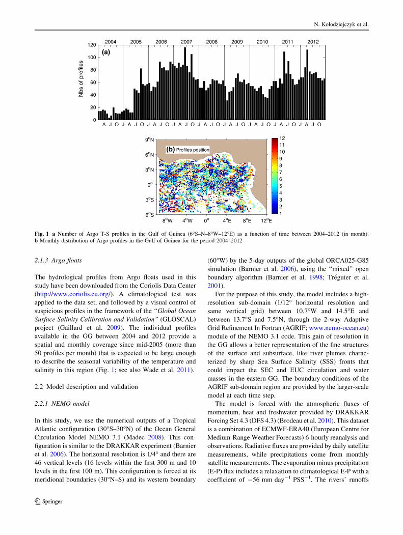
2.1.3 Argo floats

The hydrological profiles from Argo floats used in this

study have been downloaded from the Coriolis Data Center

(http://www.coriolis.eu.org/). A climatological test was

applied to the data set, and followed by a visual control of

suspicious profiles in the framework of the ‘‘Global Ocean

Surface Salinity Calibration and Validation’’ (GLOSCAL)

project (Gaillard et al. 2009). The individual profiles

available in the GG between 2004 and 2012 provide a

spatial and monthly coverage since mid-2005 (more than

50 profiles per month) that is expected to be large enough

to describe the seasonal variability of the temperature and

salinity in this region (Fig. 1; see also Wade et al. 2011).

2.2 Model description and validation

2.2.1 NEMO model

In this study, we use the numerical outputs of a Tropical

Atlantic configuration (30�S–30�N) of the Ocean General

Circulation Model NEMO 3.1 (Madec 2008). This con-

figuration is similar to the DRAKKAR experiment (Barnier

et al. 2006). The horizontal resolution is 1/4� and there are

46 vertical levels (16 levels within the first 300 m and 10

levels in the first 100 m). This configuration is forced at its

meridional boundaries (30�N–S) and its western boundary

(60�W) by the 5-day outputs of the global ORCA025-G85

simulation (Barnier et al. 2006), using the ‘‘mixed’’ open

boundary algorithm (Barnier et al. 1998; Treguier et al.

2001).

For the purpose of this study, the model includes a high-

resolution sub-domain (1/12� horizontal resolution and

same vertical grid) between 10.7�W and 14.5�E and

between 13.7�S and 7.5�N, through the 2-way Adaptive

Grid Refinement In Fortran (AGRIF; www.nemo-ocean.eu)

module of the NEMO 3.1 code. This gain of resolution in

the GG allows a better representation of the fine structures

of the surface and subsurface, like river plumes charac-

terized by sharp Sea Surface Salinity (SSS) fronts that

could impact the SEC and EUC circulation and water

masses in the eastern GG. The boundary conditions of the

AGRIF sub-domain region are provided by the larger-scale

model at each time step.

The model is forced with the atmospheric fluxes of

momentum, heat and freshwater provided by DRAKKAR

Forcing Set 4.3 (DFS 4.3) (Brodeau et al. 2010). This dataset

is a combination of ECMWF-ERA40 (European Centre for

Medium-Range Weather Forecasts) 6-hourly reanalysis and

observations. Radiative fluxes are provided by daily satellite

measurements, while precipitations come from monthly

satellite measurements. The evaporation minus precipitation

(E-P) flux includes a relaxation to climatological E-P with a

coefficient of -56 mm day-1 PSS-1. The rivers’ runoffs

A J O J A J O J A J O J A J O J A J O J A J O J A J O J A J O J A J O0

20

40

60

80

100

120

Nbs

of p

rofil

es

(a)

2004 2005 2006 2007 2008 2009 2010 2011 2012

8o oW 0oW 4 4oE 8oE 12oE 6oS

3oS

0o

3oN

6oN

9oN

(b) Profiles position

123456789101112

Fig. 1 a Number of Argo T-S profiles in the Gulf of Guinea (6�S–N–8�W–12�E) as a function of time between 2004–2012 (in month).

b Monthly distribution of Argo profiles in the Gulf of Guinea for the period 2004–2012

N. Kolodziejczyk et al.

123

are provided by the monthly climatology of Dai and Tren-

berth (2002).

The vertical turbulent mixing is parameterized using a

TKE scheme (Blanke and Delecluse 1993) with a back-

ground vertical diffusivity coefficient equal to

10-6 m2 s-1. Since convective mixing due to static insta-

bility cannot be represented in hydrostatic models, a TKE

source is added in case of density inversion in the mixed-

layer with an enhanced background vertical diffusivity

coefficient set to 10-4 m2 s-1. In the GG sub-domain

(1/12� resolution), the horizontal friction scheme is bila-

placian, applying on horizontal surfaces with a friction

coefficient equal to -1.25 9 1011 m4 s-1, while diffusion

is isopycnal and laplacian with a diffusion coefficient equal

to 100 m2 s-1.

The monthly-averaged and 5-day-averaged outputs of

the simulation for the period 1993–2007 are used in this

study. The model is started from rest on 1 January 1990.

The initial conditions for temperature and salinity were

derived from the World Ocean Atlas climatology (Antonov

et al. 2010; Locarnini et al. 2010). Only model outputs after

1993 (i.e. after 3 years of spin-up) are considered.

The present study will mostly focus of the main prop-

erties and transports within the upper thermocline (defined

as the within the rh = 24.5–26.2 isopycnal layer), where

the EUC core and the associated salinity maximum lie, or

within the thermocline (defined as the within the

rh = 24.5–26.5 isopycnal layer), where most of the EUC

transport takes place. For each 5-day output of the model,

we first determine the depths of the two isopycnals from

the linear interpolation of the vertical density profile at

each gridpoint, and then average (for mean fields) or

integrate (for transports) the model fields between these

two depths (taking into account the thickness of the vertical

grid cells). We checked that the 24.5, 26.2 and 26.5 iso-

pycnals never outcrop in the eastern equatorial Atlantic.

2.2.2 Model validation

2.2.2.1 Mean EUC Numerical results are compared with

available sections from cruises (see Tables 1 and 2) and

PIRATA moorings measurements. In order to validate the

mean state of the model, meridional sections of zonal

velocity and salinity at 10�W from the model and from the

observations described by Kolodziejczyk et al. (2009) have

been compared. It is worth noting that there were no

observations at 10�W during boreal spring in Kol-

odziejczyk et al. (2009), so the mean sections from

observations might be biased. In order to compare consis-

tently the model with the time-average of observations

from sparse sections (Fig. 2), we computed the time-

averaged sections in the model from outputs both over the

complete 1993–2007 period and at the same dates as the 17

available sections. We note that the two different ways of

averaging in the model give comparable meridional sec-

tions in zonal velocity (Fig. 2a, c) and in salinity (Fig. 2b,

d) at 10�W, indicating that an average over the 17 available

synoptic cruises is able to capture the main properties of

the circulation and of the salinity at 10�W.

In both model and observations, the mean EUC core at

10�W is located at 0.2�S around 70 m depth, within the

rh = 24.5–26.2 isopycnal layer (Fig. 2c, e); the EUC has a

larger extent in latitude in the southern hemisphere (as far

as 2�S around 50 m depth) and it extends down to at least

250 m depth. The simulated EUC has greater maximum

speed (88 cm s-1) than in observations (69 cm s-1), and

its associated eastward velocities meridional distribution is

narrower below 100 m depth. The SEC is also well com-

parable in model and observations, with maximum west-

ward velocities of about 30 cm s-1 near the surface, two

deep branches of westward velocities centered at about 3�S

and 2�N down to at least 300 m and a subsurface maximum

([10 cm s-1) in the northern deep branch of the SEC at

2�N around 100 m depth. The Guinea Current (GC) is also

present in the model, flowing eastward above 50 m depth

north of 2.5�N (Richardson and Reverdin 1987). Unfortu-

nately, there were no observations north of 2�N to validate

the model results from 2�N to the African coast.

Following Kolodziejczyk et al. (2009), two estimates of

the EUC transport are computed from the model and from

Table 2 Total (0–250 m) and upper thermocline (rh = 24.5–26.5)

EUC transports across the meridional sections of the different cruises

used in this study (Unit is Sv)

Date Section Total Transport

(Sv)

rh = 24.5–26.5

Transport (Sv)

31 July 2000 10�W 20.0 12.8

10 June 2005 10�W 20.2 14.6

13 September 2005 10�W 17.4 12.1

2 June 2006 10�W 24.4 14.6

21 November 2006 10�W 9.6 9.0

30 June 2007 10�W 9.3 8.3

23 September 2007 10�W 27.3 17.1

26 June 2005 2.8�E 11.3 8.9

22 September 2005 2.8�E 12.6 9.3

15 June 2006 2.5�E 4.3 …29 November 2006 2.4�E 11.8 9.7

14 June 2007 2.3�E 15.2 11.6

9 August 2000 0�E 11.1 5.9

11 September 2007 0�E 11.8 10.4

14 August 2000 6�E 0.0 0.0

27 September 2005 6�E 4.4 3.8

21 June 2006 6�E 1.7 1.5

8 June 2007 6�E 6.7 4.4

5 September 2007 6�E 5,6 4.3

Associated salinity maximum in the Gulf of Guinea

123

the observations (Table 2). They are defined as the integral

of eastward velocities between 2.5�S and 2�N, either in the

rh = 24.5–26.5 density range (thermocline EUC trans-

port) or in the 0–250 m depth range (total EUC transport),

for all cruises but EGEE1 and 2 cruises during which the

total EUC transport was computed only between the sur-

face and 150 m due to the limited S-ADCP depth range

(see Kolodziejczyk et al. 2009).

Despite the stronger velocity maximum in the model,

the mean total EUC transports at 10�W are comparable in

both the model (12.7 ± 7.4 Sv from individual sections;

12.8 ± 7.4 Sv with the full 15-year time series) and

observations (12.1 ± 1.9 Sv), as well as the thermocline

EUC transports from observations (8.9 ± 0.8 Sv) and from

the model (8.9 ± 3.6 Sv from individual sections;

9.3 ± 3.8 Sv with the full 15-year time series). For the

total EUC transport, this can be explained by the smaller

meridional extent of the EUC below 100 m in the model.

For the thermocline EUC transport, this results from the

smaller thickness of the thermocline layer in the model,

due to the greater mean depth of the rh = 26.5 isopycnal at

the equator in the observations (170 m) than in the model

(130 m), so that the thermocline layer (rh = 24.5–26.5

density range) encompasses a larger portion of the EUC in

the observations (Fig. 2c, e). It is worth mentioning that the

stratification below the thermocline appears to be more

diffuse in the model than in the in situ data.

The salinity maximum associated with the EUC core

reaches 36.18 in the model, and 36.00 PSS in the obser-

vations (Fig. 2d, f). This positive bias around 0.18 PSS in

the model is found to occur over the whole rh = 24.5–26.5

isopycnal range between 5�S and 2�N, indicating that

salinities are generally too strong in the simulated equa-

torial thermocline. Nevertheless, the mean latitudinal dis-

tribution of salinity within the upper thermocline agrees

qualitatively in the model and in the observations. Both

(a) (b)

(c) (d)

(e) (f)

Fig. 2 Mean meridional

sections at 10�W of zonal

currents (left) and salinity

(right) in the model (a–d) and

from observations

(e–f) (Kolodziejczyk et al.

2009; their Table 2). To

facilitate the comparison with

the observations, the time-

averaged sections from the

model have been computed

from the full 1993–2007 period

(a, b) and from the outputs at

the same dates as the 17

hydrographical sections in

Kolodziejczyk et al. (2009)

(c, d). Currents are in cm s-1.

Thick black lines refer to the

zero isotach in (a), (c) and (e),

and to 35.0, 35.5 and 36.0

isohalines in (b), (d) and (f).Isopycnals 24.5, 26.2, 26.5 and

26.8 are superimposed in solid

white lines. Black dots in

(a–d) represent the vertical grid

of the model

N. Kolodziejczyk et al.

123

sections show (i) a well-defined salinity maximum asso-

ciated with the EUC core in the upper thermocline layer

(rh = 24.5–26.2) slightly south of the equator, (ii) stronger

salinities along the rh = 24.5 isopycnal in the southern

hemisphere than north of the equator, (iii) the presence of a

second salinity maximum around 50 m depth along the

rh = 24.5 isopycnal south of 4�S, which is the signature of

subtropical waters originating from the southern hemi-

sphere (Kolodziejczyk et al. 2009), and (iv) a sharp halo-

cline around 40 m depth in the northern hemisphere, with

surface salinities lower than 35.4 PSS.

2.2.2.2 Seasonal variability at the equator

(a) Zonal velocity

In the Atlantic Ocean, the EUC exhibits a robust seasonal

cycle between 35�W and 0�E both in observations (e.g.,

Brandt et al. 2006; Kolodziejczyk et al. 2009; Johns et al.

2014) and in models (e.g., Arhan et al. 2006). In order to

get more insight into the ability of our model to reproduce

the seasonal variability of EUC velocities, we compare the

mean seasonal cycle of equatorial zonal velocities at 10�W

in the model (Fig. 3b) with the mean seasonal cycle

derived from ADCP measurements from the PIRATA

mooring between June 2003 and December 2007 (Fig. 3a).

The ADCP measurements suffer from one important gap

between June 2005 and May 2006, and were available only

in the first 100 m in 2006–2007. However, the period of

PIRATA observations encompasses at least 3 complete

years in the upper 100 m, which is likely enough to capture

the predominant features of the seasonal cycle.

In the upper 100 m, the zonal velocities are generally

stronger (of about 10–20 cm s-1) in the model than in the

PIRATA mooring, while they are somewhat less intense

below 150 m. However, the seasonal evolution and vertical

structure of the zonal velocities are qualitatively repro-

duced in the model: (i) the depth of the EUC core ranges

between 50 and 70 m depth, shallowing during the boreal

winter and spring and deepening in summer and fall; (ii)

the EUC core is encompassed throughout the year in the

upper thermocline, between rh = 24.5 and rh = 26.2 is-

opycnals; (iii) above 50 m depth, the eastward velocities

associated with the EUC extend upward to the surface

during September, in agreement with the annual weaken-

ing/reversal of the SEC (Ding et al. 2009); (iv) below

150 m depth, an annual reversal of the zonal current is

found (though of lesser amplitude in the model), with

predominantly eastward velocities from April to September

and westward velocities from October to March.

(b) Salinity and temperature

Then, we compare the mean seasonal variability of the

salinity maximum computed with the model (Fig. 4c, d)

and computed from PIRATA moorings data at 10�W–0�N

and 0�E–0�N between 1998 and 2012 (Bourles et al. 2008;

Fig. 4a, b).

At both longitudes the salinity seasonal cycle is quali-

tatively well reproduced in the model: (i) the salinity

maximum associated with the EUC is present between 40

and 80 m, and is located throughout the year between the

rh = 24.5 and rh = 26.2 isopycnals; (ii) the strong annual

cycle in surface salinity, and in the vertical gradient of

salinity between the surface and 50 m depth, is comparable

in the model and in the observations, with weakest values

in February–May and strongest values in boreal summer

and fall. (iii) this salinity maximum is subject to a semi-

annual variability, with maximum salinity in April and

October–November, but the intense weakening of the

salinity maximum in December at 10�W is not reproduced

in the model. However, as previously noted in the mean

salinity section at 10�W, there is a constant bias in salinity

in the model, the simulated salinity of the upper layer of the

equatorial GG being about 0.2 PSS saltier than the

observed one. This constant bias however does not affect

the seasonal variability of near-surface salinities in the

model.

The seasonal cycles of temperature at 10�W and 0�E in

the model (Fig. 5c, d) also display a qualitative good

−100 cm.s−1

−80

−60

−40

−20

0

20

40

60

80

100

24.5 24.5

26.2 26.2

26.5 26.5

Dep

th (

m)

(b) 10°W − U−MODEL

J F M A M J J A S O N D250

200

150

100

50

0

Dep

th (

m)

24.524.5

26.226.2

(a) 10°W − U−DATA

250

200

150

100

50

0

Fig. 3 Climatological Month-depth evolution of the zonal velocities

(in cm s-1) between 0–250 m depth at 0�N–10�W (a) from available

currentmeters data between 2003 and 2007, and (b) from NEMO

model output between 1993 and 2007. Isopycnals 24.5, 26.2, and 26.5

are superimposed in solid white lines. Black dots in (b) represent the

vertical grid of the model

Associated salinity maximum in the Gulf of Guinea

123

agreement with the seasonal cycles derived from PIRATA

moorings at 10�W and 0�E (Fig. 5a, b): (i) the 20 �C iso-

therm is located around 70 m depth during boreal winter–

spring and 40–50 m depth during the boreal summer; (ii)

the depth of the thermocline experienced a clear semi-

annual cycle, being shallower during late boreal spring and

summer, and with a lesser amplitude in December at both

longitudes; (iii) the 24.5–26.2 isopycnal layer encompasses

the strongest vertical gradient of temperature of the upper

thermocline throughout the year; (iv) at 0�E, the thermo-

cline is sharper during boreal summer in both data and

model.

As for the zonal velocities, the model thus reproduces

qualitatively well the observed water masses properties,

their vertical distribution and their seasonal variability in

the upper layers at 0�N–10�W and 0�N–0�E.

(c) EUC transport

To assess the ability of the model to reproduce realistic

EUC transports in the eastern Atlantic ocean, Fig. 6 pre-

sents scatter plots of the total and thermocline EUC

transports estimated from the available synoptic meridional

sections over the period 1999–2007 at 10�W, *1�E and

6�E, and the corresponding estimates from the model at the

same longitudes and dates. At 10�W and 1�E, the total

(Fig. 6a) and thermocline (Fig. 6b) EUC transports are

reasonably simulated for the values that are close to the

mean values (squares), i.e. for transports between 5 and

20 Sv. Nevertheless, the largest total and thermocline EUC

transports in the observations (beyond 20 Sv at 10�W and

12 Sv at *1�E, respectively) are systematically lower in

the model. Along 6�E (red circles), the EUC transports are

generally too intense in the model.

To put these estimates for the EUC transport in the

context of the seasonal variability, Fig. 7 presents the mean

monthly evolution of the total and thermocline EUC

transports (solid), their standard deviation (STD; gray

shaded) and their maximum/minimum (dashed lines) in the

model, along with the corresponding estimates from

available observations (black dots), at 10�W, 1�E and 6�E.

The standard deviation, the minimum and maximum of

EUC transports have been computed for each calendar

month from the 5-day outputs of the model over the period

1993–2007.

At 10�W (Fig. 7a, b), 17 different estimates of the EUC

transport spanning the whole year are available from

Kolodziejczyk et al. (2009) (see their Table 2 for more

details). Note however that most cruises took place from

June to September and from November to February, with

only one estimate for the total EUC transport during boreal

24.524.5

26.226.2

24.5 24.5

26.2 26.2

5

24.5 24.5

26.226.2

24.5

24.524.5

26.2

26.226.2

24.524.5

26.226.2

24.5 24.5

26.2 26.2

5

24.5 24.5

26.226.2

24.5

24.524.5

26.2

26.226.2

24.524.5

26.226.2

(b) 0°E − S−DATA

24.5 24.5

26.2 26.2

5

Dep

th (

m)

(c) 10°W − S−MODEL

J F M A M J J A S O N D120

100

80

60

40

20

0

24.5 24.5

26.226.2

(d) 0°E − S−MODEL

J F M A M J J A S O N D

33 PSS33.233.433.633.83434.234.434.634.83535.235.435.635.83636.236.436.636.837

24.5

24.524.5

26.2

26.226.2

Dep

th (

m)

(a) 10°W − S−DATA120

100

80

60

40

20

0

Fig. 4 Climatological Month-depth evolution of the salinity (in PSS)

between 0–120 m depth (a, b) from available PIRATA salinity data

between 1998 and 2013 and (c, d) from NEMO model output between

1993 and 2007, at 0�N–10�W (a–c) and 0�N–0�E (b–d). Isopycnals

24.5 and 26.2 are superimposed in solid white lines. Black dots in (c,

d) represent the vertical grid of the model

N. Kolodziejczyk et al.

123

spring (no CTD data during this cruise) and no observation

in October. The observations and the model indicate a

yearly maximum of both total and thermocline EUC

transports in August–September and a yearly minimum

during November–December, as confirmed from moored

current-meters by Johns et al. (2014). The model further

exhibits a very weak maximum during the boreal spring

that agrees with the observations by Johns et al. (2014), but

cannot be evidenced from the unique synoptic section

available during this season. The transport estimates from

observations exhibit a maximum range of variability during

boreal summer and a minimum range during November–

December that roughly agree with the minimum/maximum

transports computed from the 5-day model output (Fig. 7).

The cruise-to-cruise variability is lower in boreal fall and

winter than during boreal summer, suggesting less intra-

seasonal or interannual variability of the EUC transport

during this period.

24.524.5

26.226.2

24.5 24.5

26.2 26.2

5

24.5 24.5

26.226.2

24.524.5

26.226.2

24.524.5

26.226.2

(b) 0°E − T−DATA

24.5 24.5

26.2 26.2

5

Dep

th (

m)

(c) 10° W − T−MODEL

J F M A M J J A S O N D120

100

80

60

40

20

0

24.5 24.5

26.226.2

(d) 0°E − T−MODEL

J F M A M J J A S O N D

10° C

12

14

16

18

20

22

24

26

28

3024.524.5

26.226.2

Dep

th (

m)

(a) 10°W − T−DATA120

100

80

60

40

20

0

Fig. 5 Same as Fig. 4, except for temperature

(a) (b)

Fig. 6 Comparison of the individual a total and b thermocline

(rh = 24.5–26.5) EUC transports estimated from the different cruises

and from the model, at 10�W (black dots), 0�E (blue dots) and 6�E

(red dots). Cruises are described in Kolodziejczyk et al. (2009) and in

Table 2. The squares represent the mean values at each longitude.

The Total Root Mean Square Deviation (RMSD) and linear fit

(dashed line) are indicated in each sub-figure

Associated salinity maximum in the Gulf of Guinea

123

At 1�E and 6�E (Fig. 7c–f), observations are available

only from June to November, and in limited number. For

this period, both model and observations indicate that the

total and thermocline EUC transports weaken from 10�W

to 6�E (Fig. 6b, d, f). Note in particular that the transport

almost vanishes at 6�E during one cruise in August 2000

(see also Bourles et al. 2002). Moreover, in agreement with

observations by Johns et al. (2014), the total and thermo-

cline EUC transports in the model exhibit a seasonal

maximum in April at 1�E, but no cruise is available during

this season.

3 Evidence of a westward recirculation of the EUC

salinity maximum in June 2007

In this section, we focus on the observations of currents,

salinity and dissolved oxygen acquired in June 2007 in the

Gulf of Guinea during the EGEE5 cruise (Fig. 8). The

meridional sections of salinity along 10�W, 2.3�E and 6�E

(Fig. 8d–f) reveal, within the upper thermocline layer

(defined here between the 24.5 and 26.2 isopycnals), the

presence of high salinities (exceeding 36.0) both at the

equator and off the equator (near 3�N and 3�S at 2.3�E), as

previously evidenced by Gouriou and Reverdin (1992). At

the equator, high salinities are observed along the three

sections at the depth of the EUC core (Fig. 8d–f) and

coincide with high dissolved oxygen concentrations (up to

120 lmol kg-1; Fig. 8g–i). At 10�W, it is worth noticing

that the strong salinities that are visible south of 4.5�S

around the 24.5 isopycnal (Fig. 8a, d), in the region of the

eastward South Equatorial Undercurrent (SEUC) do not

result from the recirculation of the EUC in the eastern GG.

They are likely the signature of the subtropical water

masses from the south Atlantic advected by the SEUC

(Kolodziejczyk et al. 2009), and are thus beyond the scope

of the present study.

The EUC maximum velocity decreases eastward from

70 cm s-1 to 40 cm s-1 (Fig. 8d–f), while the thermocline

EUC transport first increases from 8.3 Sv to 11.6 Sv

between 10�W and 2.3�E, and subsequently decreases to

4.4 Sv at 6�E. Note that both eastward velocities and high

oxygen concentrations extend below rh = 26.2 (down to

the 26.5 isopycnal) at 10�W and 2.3�E, i.e. deeper than the

salinity maximum of the EUC core which is confined to the

upper thermocline (Fig. 8d, g).

At 6�E, salinities exceeding 35.9 and dissolved oxygen

concentrations greater than 150 lmol kg-1 cover the

whole latitude range of the meridional section (between

1�S to 2.5�N) in the upper thermocline (Fig. 8i), in contrast

with the EUC that remains confined between 1�N and 1�S

(Fig. 8c). Between 1�N and 2.5�N, high salinities are

associated with a westward current, which strongly sug-

gests that EUC water masses spread poleward and recir-

culate westward near that longitude.

At 2.3�E, this extra-equatorial westward recirculation of

EUC water masses is more clearly identified through the

presence of two maxima of salinity (up to 36.2) and oxygen

0

10

20

30

Sv

Total EUC transport

(a) 10°W

Thermocline EUC transport

(b) 10°W

0

5

10

15

20

Sv

(c) 1°E (d) 1°E

J F M A M J J A S O N D0

5

10

15

Sv

(e) 6°E

J F M A M J J A S O N D

(f) 6°E

Fig. 7 Seasonal variability of

the EUC transport (in Sv) in the

model: total transport

(0–250 m) (left) and

thermocline transport

(rh = 24.5–26.5) (right), at

10�W (upper), 1�E (middle) and

6�E (lower). Black curves

represent the monthly mean

transport, during the period

1993–2007. Standard deviation

for the monthly transports

(calculated from the 5-day

output) is superimposed in gray.

Dashed lines refer to maximum

and minimum values taken from

the 5-day output for each

month. Circles represent the

individual estimates from

observations in Kolodziejczyk

et al. (2009) (their Table 2) and

in this study (Table 2)

N. Kolodziejczyk et al.

123

(140 lmol kg-1) near 3�S and 3�N, with values compara-

ble with those at 6�E. Contrary to 6�E, the high salinity

cores off the equator are clearly distinct from the equatorial

salinity maximum related to the EUC core (Fig. 8e). The

total transports of these westward flows within the upper

thermocline are 5.5 and 2.0 Sv respectively north and south

of the equator, leading to a total extra-equatorial westward

transport of 7.5 Sv in the upper thermocline. These results

are comparable with the observations made in March 1995

at 3�E by Mercier et al. (2003).

At 10�W, a westward current is still found in the ther-

mocline between 1�S and 3�S (Fig. 8a). This current is still

associated with a relative maximum of oxygen (up to

120 lmol kg-1), but no longer with a local salinity maxi-

mum. However, the horizontal distribution of salinity and

oxygen in the upper thermocline at 2.3�E and 10�W around

3�S strongly suggests the continuity of the westward extra-

equatorial circulations of saline water masses originating

from the EUC.

4 Seasonal variability of the upper EUC water masses

We now focus on the time evolution of vertical average of

salinity and the zonal transport in the upper thermocline

(rh = 24.5–26.2 isopycnal range)—i.e. where the salinity

maximum associated with the EUC core is confined—as

observed from all the individual Argo profiles available

from 2004 to 2012 (Fig. 9) and seven cruises available

from June to November between 2000 and 2007 (Fig. 10).

In the GG, the coverage of Argo profiles is sufficient to

depict the climatological seasonal variability of the mean

salinity within the upper thermocline (Fig. 9). In spite of

possible intra-seasonal and inter-annual variability in the

data, a robust seasonal cycle is observed. From January–

February to May–June (Fig. 9a–c), the upper thermocline

is characterized by a tongue of high saline water masses

(up to 36.1 PSS) along the equator (within a ±1.5� latitude

band) extending over the whole GG. In the eastern GG,

these saline water masses progressively spread off the

equator, and westward along 3�N–S until May–June.

During July–August (Fig. 9d), the mean salinity in the

upper thermocline dramatically weakens down to 35.7 PSS

along the equator, while the extra equatorial maxima of

salinity remain present east of 0�E. From September–

October (Fig. 9e–f), the equatorial salinity maximum first

reforms west of 0�E, before extending again over the whole

GG in November–December (Fig. 9f), while the extra-

equatorial maxima progressively disappear during this

season.

Fig. 8 Meridional sections at 10�W (left column), 2.3�E (central

column) and 6�E (right column) of zonal velocity (upper; in cm s-1;

isotach 0 in bold), salinity (middle) and dissolved oxygen (lower; in

lmol kg-1) as measured during the EGEE5 cruise in June 2007.

Isopycnals 24.5, 26.2, 26.5 and 26.8 are superimposed in solid white

lines

Associated salinity maximum in the Gulf of Guinea

123

6oS

3oS

0o

3oN

6oN

9oN

(a) Jan/Feb

S ARGO σθ = 24.5−26.2

(b) Mar/Apr (c) May/Jun

8oW 4oW 0o 4oE 8oE 12oE 6oS

3oS

0o

3oN

6oN

9oN

(d) Jul/Aug

8oW 4oW 0o 4oE 8oE 12oE

(e) Sep/Oct

35.7 PSS

35.8

35.9

36

36.1

8oW 4oW 0o 4oE 8oE 12oE

(f) Nov/Dec

Fig. 9 Bi-monthly climatology of mean upper thermocline salinity (shaded color; in PSS) from each available Argo profiles in the GG between

2004 and 2012. Months from January/February (a) to November/December (f) are indicated in each subfigure

Fig. 10 Zonal transport per

0.5� of latitude (arrows; in Sv)

and mean salinity (color; in

PSS) in the upper thermocline

(24.5–26.2 isopycnal layer)

during each cruise. The month

and year of each cruise are

indicated in each subfigure.

Scaling for transport and

salinity is provided in the

bottom/right

N. Kolodziejczyk et al.

123

The seven cruises carried out in the GG between 2000

and 2007 allow us to describe the salinity and the associ-

ated horizontal transport distribution during the summer to

fall season. During June 2006 and 2007, the year-to-year

distribution of salinity and transport presents qualitatively

common features (Fig. 9a, b), e.g. the EUC is observed

along the equator from 10�W to 6�E with salinities greater

than 35.9. As described in the previous section, westward

recirculations are observed north and south of the equator

in June 2007 at 2.3�E and north of the equator at 6�E,

transporting salty waters with comparable salinity values as

for the EUC at the equator (Fig. 9b). A similar recircula-

tion is suggested north of the equator across 6�E and 2.5�E

in June 2006 (Fig. 10a), but there is no data for this cruise

to confirm its existence in the southern hemisphere. During

June 2006 and 2007, the salinity distribution agrees qual-

itatively well with the seasonal one given from Argo data

(Fig. 9c).

Nevertheless, during June 2005 and August 2000

(Fig. 10c, d), the salinity distribution clearly differ from the

seasonal picture given from Argo data during May–June

(Fig. 9c) and July–August (Fig. 9d), whereas the horizontal

distribution of transports are alike during June 2005 and

August 2000. During both cruises, the EUC is only present

at 10�W, but the associated salinity maximum is weaker

than the corresponding bi-monthly distribution suggested

in Argo data. At 2.3�E (in June 2005) and 0�E (in August

2000), zonal transports at the equator are weak, even

westward, suggesting that the upper EUC does not pene-

trate in the eastern GG during these two cruises. In June

2005 at 2.3�E, extra-equatorial salinity maxima are weaker

than the ones obtained in May–June from Argo data, and

associated with weak westward transports. In August 2000

at 6�E, weak extra-equatorial salinity maxima are observed

on both sides of the equator near 3�S and 3�N, associated

with eastward flows. The June 2005 and August 2000

cruises data strongly suggest that interannual variability

may strongly modulate the mean seasonal variability

deduced from Argo measurements.

In September 2005 and 2007 and November 2006

(Fig. 9e–g), the EUC is again observed in the upper ther-

mocline with a high salinity signature, in agreement with

salinity Argo distribution during this year period (Fig. 9e,

f). In early September (2007; Table 1), the upper EUC does

not reach 6�E and salinity is weaker than 35.8 near 0�E

(Fig. 10e). In contrast, in late September (2005; Table 1),

the EUC is present from 10�W to 6�E, and carries salinity

of about 35.9 at 2.3�E and 6�E (Fig. 9f). In November 2006

(Fig. 10g), the EUC is associated with salinities greater

than 36.0 at 2.3�E. This suggests a progressive eastward

penetration of the EUC and saline water masses along the

equator from late boreal summer to mid boreal fall, thus

supplying again the GG with high salinity waters of

subtropical origin. In agreement with Argo data, neither

salinity maximum nor intense westward recirculations are

observed off the equator during these three cruises.

5 Seasonal variability of the EUC termination

in the model

5.1 EUC termination and circulation of saline water

masses

To infer in more details the horizontal structure of the

upper thermocline circulation in the GG and overview its

complete seasonal cycle, we now analyze the bi-monthly

climatological horizontal distribution of mean salinity and

transports within the upper thermocline, calculated from

the 1993–2007 NEMO simulation (Fig. 11).

From May to November (Fig. 11c–f), the seasonal

evolutions of zonal transport and salinity in the upper

thermocline are qualitatively in good agreement with the

descriptions provided in the previous section: (i) the EUC

slightly weakens from May, then strongly diminishes and

disappears east of 5�E during July–August (Fig. 11c–d). It

strengthens in September–October when it is present again

until the African coast (Fig. 11e); (ii) extra-equatorial

westward transport are intensified between 2� and 3� in

both hemispheres from May to July (Fig. 11c–d); (iii) a

strong salinity maximum is present near the equator in

May–June (Fig. 11c), is largely eroded in July–August

(Fig. 11d) and reappears from the west in September

(Fig. 11e); (iv) extra-equatorial salinity maxima are

observed from May to August near 3�N and 3�S (Fig. 11c,

d). These extra-equatorial high salinities are spatially

connected to the EUC salinity maximum in May–June in

the eastern half of the GG (Fig. 11c). Then they persist in

time, despite the disappearance of the EUC salinity maxi-

mum in boreal summer, until appearing as local salinity

maxima near 4�S and 4�N in July–August. During late

summer and fall, the southern salinity maximum slightly

moves southward, probably advected by the poleward

transport (Fig. 11d–f). The close qualitative agreement

between the bi-monthly climatology from the model and

the in situ observations (Figs. 9, 10) confirms that the

model is able to reasonably reproduce the salient features

of the seasonal cycle in the upper thermocline.

The model outputs allow us also to describe the poorly

documented variability of the upper EUC termination and

salinity from November to May. During this period, the

upper EUC transports high subtropical saline waters along

the equator to the eastern GG (Fig. 11f, a–c). At the

African coast the EUC flow and its associated saline waters

bifurcate meridionally and progressively reform the extra-

equatorial maxima between 1.5–3.5�N–S. From January–

Associated salinity maximum in the Gulf of Guinea

123

May, the extra-equatorial westward flow in the upper

thermocline transports the saline waters masses westward

(Fig. 11a–c).

Note that, in the southern hemisphere a very small

poleward transport along the African coast is observed in

the upper thermocline, amounting to only 0.2 ± 0.6 Sv

across 5�S between 9�E and the coast. Between May and

August, the southward export along the African coast is

0.2 Sv while the salinity maximum is eroded in this region.

This transport along the African coast is even observed to

reverse in September–November (*0.2 Sv northward),

while the salinity is minimum. The poleward transport is

maximum during the winter (*0.4 Sv in December–Feb-

ruary), while the salinity re-increases south of the equator

along the African coast. Thus, although a direct export of

EUC water masses along the African coast found in the

model in the coastal GCUC, as previously suggested by

Wacongne and Piton (1992), it only represents a very small

part of the EUC transport. The EUC recirculates primarily

in the westward extra-equatorial branches of the SEC.

In order to better describe the seasonal evolution of the

upper thermocline in the GG, we computed the monthly

climatology of the depth of the thermocline (materialized

here by rh = 26.2 isopycnal depth), the vertically-aver-

aged salinity and the zonal transport in the upper thermo-

cline in time-latitude diagrams along 1�E in the center of

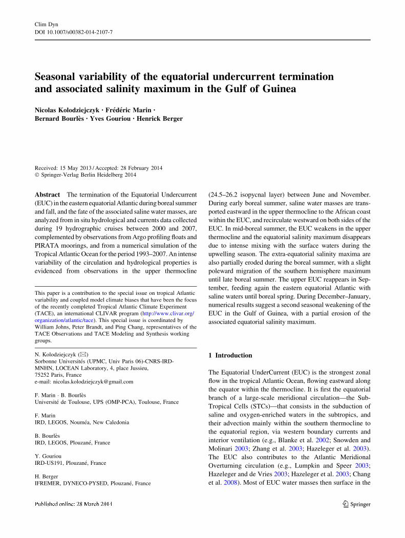
the GG (Fig. 12). At the equator, the depth of the

rh = 26.2 and the salinity both exhibit two minima during

a climatological year, with the salinity lagging the

rh = 26.2 depth by about 1 month (Fig. 12a, b). For

instance, a first strong minimum in the rh = 26.2 depth is

observed from June–July to September, while it is observed

from July to October for the salinity. The rh = 26.2 depth

experiences a second weaker minimum in December,

leading the second salinity relative minimum observed in

January (Fig. 12a, b). On the other hand, the upper EUC

transport shows only one minimum in July–August

(Fig. 12c).

Off the equator, the rh = 26.2 depth is also subject to a

semi-annual cycle, with a first strong maximum in March–

April and a second maximum of weaker amplitude in

October–November (Fig. 12a). In contrast, the extra-

equatorial salinity exhibits a dominant annual cycle, with

minimum values from September to January (Fig. 12b). At

the equator during the late spring, the salinity decreases

concomitantly to the rh = 26.2 depth and transport, and

leads the more progressive poleward erosion of the salinity

maxima. Off the equator, from December until the fol-

lowing summer, the salinity maxima are reformed around

2.5�N–S, concomitantly to the deepening of the rh = 26.2

depth and the increase of the westward transports

(Fig. 12a–c).

The cycle of these three quantities suggests different

processes for the boreal summer erosion of the salinity

maxima in the GG. At the equator, the strong shallowing of

the upper thermocline may contribute to bring its waters

near the surface and to increase the vertical shear between

the EUC and the surface westward SEC, leading to an

enhanced mixing with the surface fresher waters. On the

other hand, the dramatic weakening of the EUC transport,

starting in late boreal spring, interrupts the supply of saline

waters toward the GG. In order to get more insight into the

contribution of both advection and mixing in the erosion of

saline water, we have computed, in the next section, the

(a) Jan/Feb

MEAN σθ = 24.5−26.2

(b) Mar/Apr (c) May/Jun

8oW 4oW 0o 4oE 8oE 12oE

(d) Jul/Aug

8oW 4oW 0o 4oE 8oE 12oE

(e) Sep/Oct

35.7 PSS

35.8

35.9

36

36.1

8oW 4oW 0o 4oE 8oE 12oE

(f) Nov/Dec2 Sv/1°

Fig. 11 Bi-monthly climatology of the transport per unit of latitude/

longitude (arrows; scaling provided in the bottom/right panel) and

mean salinity (shaded color) in the 24.5–26.2 isopycnal layer in the

model. Months from January/February (a) to November/December

(f) are indicated in each subfigure

N. Kolodziejczyk et al.

123

seasonal salinity budget in the upper thermocline of the

eastern GG.

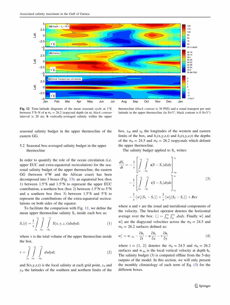
5.2 Seasonal box-averaged salinity budget in the upper

thermocline

In order to quantify the role of the ocean circulation (i.e.

upper EUC and extra-equatorial recirculation) for the sea-

sonal salinity budget of the upper thermocline, the eastern

GG (between 4�W and the African coast) has been

decomposed into 3 boxes (Fig. 13): an equatorial box (box

1) between 1.5�S and 1.5�N to represent the upper EUC

contribution, a northern box (box 2) between 1.5�N to 5�N

and a southern box (box 3) between 1.5�S and 5�S to

represent the contributions of the extra-equatorial recircu-

lations on both sides of the equator.

To facilitate the comparison with Fig. 11, we define the

mean upper thermocline salinity Sm inside each box as:

SmðtÞ ¼1

m

Z

yN

yS

Z

xE

xW

Z

�h1

�h2

Sðx; y; z; tÞdxdydz ð1Þ

where m is the total volume of the upper thermocline inside

the box.

m ¼Z

yN

yS

Z

xE

xW

Z

�h1

�h2

dxdydz ð2Þ

and S(x,y,z,t) is the local salinity at each grid point, yS and

yN the latitudes of the southern and northern limits of the

box, xW and xE the longitudes of the western and eastern

limits of the box, and h1(x,y,z,t) and h2(x,y,z,t) the depths

of the rh = 24.5 and rh = 26.2 isopycnals which delimit

the upper thermocline.

The salinity budget applied to St writes:

dSm

dt¼ � 1

m

Z

yN

yS

Z

�h1

�h2

uðS� SmÞdzdy

2

6

4

3

7

5

xE

xW

� 1

m

Z

xE

xW

Z

�h1

�h2

vðS� SmÞdzdx

2

6

4

3

7

5

yN

yS

� 1

mwc

1ðS1 � SmÞ� �

þ 1

mwc

2ðS2 � SmÞ� �

þ Res

ð3Þ

where u and v are the zonal and meridional components of

the velocity. The bracket operator denotes the horizontal

average over the box: :h i ¼R xE

xW

R yN

yS:dxdy: Finally w1

c and

w2c are the diapycnal velocities across the rh = 24.5 and

rh = 26.2 surfaces defined as:

wci ¼ w�hi

� ohi

ot� u

ohi

ox� v

ohi

oyð4Þ

where i = {1, 2} denotes the rh = 24.5 and rh = 26.2

surfaces and w-hi is the local vertical velocity at depth hi.

The salinity budget (3) is computed offline from the 5-day

outputs of the model. In this section, we will only present

the monthly climatology of each term of Eq. (3) for the

different boxes.

−4 Sv/1°−3−2−10123

Lat.

(c) Zonal Transport per unit latitude

1°E

Jan Feb Mar Apr May Jun Jul Aug Sep Oct Nov Dec Jan−5

−2.5

0

2.5

5

50 m depth

60

70

80

90

100

110

120

Lat.

(a) Depth − σθ = 26.2

1°E−5

−2.5

0

2.5

5

35.86 PSS35.935.9435.9836.0236.0636.136.1436.18

Lat.

(b) Salinity

1°E−5

−2.5

0

2.5

5

Fig. 12 Time-latitude diagrams of the mean seasonal cycle at 1�E

between 5�S–N of a rh = 26.2 isopycnal depth (in m, black contour

interval is 20 m), b vertically-averaged salinity within the upper

thermocline (black contour is 36 PSS) and c zonal transport per unit

latitude in the upper thermocline (in Sv/1�, black contour is 0 Sv/1�)

Associated salinity maximum in the Gulf of Guinea

123

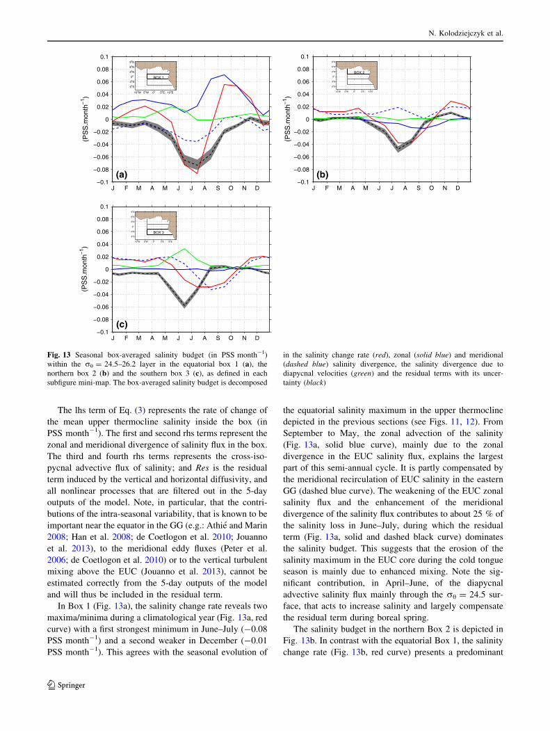
The lhs term of Eq. (3) represents the rate of change of

the mean upper thermocline salinity inside the box (in

PSS month-1). The first and second rhs terms represent the

zonal and meridional divergence of salinity flux in the box.

The third and fourth rhs terms represents the cross-iso-

pycnal advective flux of salinity; and Res is the residual

term induced by the vertical and horizontal diffusivity, and

all nonlinear processes that are filtered out in the 5-day

outputs of the model. Note, in particular, that the contri-

butions of the intra-seasonal variability, that is known to be

important near the equator in the GG (e.g.: Athie and Marin

2008; Han et al. 2008; de Coetlogon et al. 2010; Jouanno

et al. 2013), to the meridional eddy fluxes (Peter et al.

2006; de Coetlogon et al. 2010) or to the vertical turbulent

mixing above the EUC (Jouanno et al. 2013), cannot be

estimated correctly from the 5-day outputs of the model

and will thus be included in the residual term.

In Box 1 (Fig. 13a), the salinity change rate reveals two

maxima/minima during a climatological year (Fig. 13a, red

curve) with a first strongest minimum in June–July (-0.08

PSS month-1) and a second weaker in December (-0.01

PSS month-1). This agrees with the seasonal evolution of

the equatorial salinity maximum in the upper thermocline

depicted in the previous sections (see Figs. 11, 12). From

September to May, the zonal advection of the salinity

(Fig. 13a, solid blue curve), mainly due to the zonal

divergence in the EUC salinity flux, explains the largest

part of this semi-annual cycle. It is partly compensated by

the meridional recirculation of EUC salinity in the eastern

GG (dashed blue curve). The weakening of the EUC zonal

salinity flux and the enhancement of the meridional

divergence of the salinity flux contributes to about 25 % of

the salinity loss in June–July, during which the residual

term (Fig. 13a, solid and dashed black curve) dominates

the salinity budget. This suggests that the erosion of the

salinity maximum in the EUC core during the cold tongue

season is mainly due to enhanced mixing. Note the sig-

nificant contribution, in April–June, of the diapycnal

advective salinity flux mainly through the rh = 24.5 sur-

face, that acts to increase salinity and largely compensate

the residual term during boreal spring.

The salinity budget in the northern Box 2 is depicted in

Fig. 13b. In contrast with the equatorial Box 1, the salinity

change rate (Fig. 13b, red curve) presents a predominant

J F M A M J J A S O N D−0.1

−0.08

−0.06

−0.04

−0.02

0

0.02

0.04

0.06

0.08

0.1

(PS

S.m

onth

−1 )

(a)

BOX 1

10oW 5oW 0o 5oE 10oE

6oS

3oS

0o

3oN

6oN

9oN

J F M A M J J A S O N D−0.1

−0.08

−0.06

−0.04

−0.02

0

0.02

0.04

0.06

0.08

0.1

(PS

S.m

onth

−1 )

(b)

BOX 2

10oW 5oW 0o 5oE 10oE

6oS

3oS

0o

3oN

6oN

9oN

J F M A M J J A S O N D−0.1

−0.08

−0.06

−0.04

−0.02

0

0.02

0.04

0.06

0.08

0.1

(PS

S.m

onth

−1 )

(c)

BOX 3

10oW 5oW 0o 5oE 10oE

6oS

3oS

0o

3oN

6oN

9oN

Fig. 13 Seasonal box-averaged salinity budget (in PSS month-1)

within the rh = 24.5–26.2 layer in the equatorial box 1 (a), the

northern box 2 (b) and the southern box 3 (c), as defined in each

subfigure mini-map. The box-averaged salinity budget is decomposed

in the salinity change rate (red), zonal (solid blue) and meridional

(dashed blue) salinity divergence, the salinity divergence due to

diapycnal velocities (green) and the residual terms with its uncer-

tainty (black)

N. Kolodziejczyk et al.

123

annual cycle characterized by a salinity increase from

October to April (maximum 0.02 PSS month-1), and a

salinity decrease from May to October (minimum -0.04

PSS month-1). During the winter–spring season, the

salinity increase is mainly explained by the meridional

advection of salinity into the box (Fig. 13b, dashed blue

curve), while during the boreal late spring and summer, the

loss is mainly explained by the residual term (Fig. 13b,

dashed black curve), i.e. mixing. The diapycnal flux of salt

remains negligible throughout the year (Fig. 13b, green

curve).

In the southern Box 3 (Fig. 13c) as for the northern box 2,

the salinity change rate (Fig. 13c, red curve) shows a domi-

nant annual cycle with a freshening from May to October

(minimum -0.03 PSS month-1), and an increase of salinity

from September to April (maximum 0.02 PSS month-1), i.e.

in phase with the northern and equatorial boxes. The merid-

ional advection of salinity (dashed blue curve) from the EUC

recirculation explains the salinity increase from October to

April as for the two other boxes. In contrast, from August to

October, the meridional advection of salinity across 5�S is the

main contributor to the freshening. This freshening can be

explained by the southward displacement, in late summer and

fall, of the southern salinity maximum, that is observed in the

south–eastern part of the GG around 4–6�S in Fig. 11d, e. The

residual term only contributes from April to August, partic-

ipating to the erosion of the salinity maximum in boreal

summer, and is partly compensated by the cross-isopycnal

advective flux.

In summary, the strong diminution of salinity noticed

during the late spring and summer in the equatorial box 1 is

firstly explained by the residual term. This term represents the

vertical and horizontal mixing that contributes to the bulk of

erosion in the upper equatorial thermocline (about 75 %),

plus the possible effect of meridional eddy flux due to intra-

seasonal variability. The dramatic weakening of the salinity

advection by the EUC at 4�W contributes also to about 25 %

of the diminution of equatorial salinity. In the extra-equato-

rial boxes, the mixing term appears also to play a dominant

role in eroding the salinity maxima during the late spring and

summer, while meridional advection acts to supply extra-

equatorial maxima of salinity with saline waters from the

EUC in winter and spring. It is also interesting to note the

north–south asymmetry during the erosion of extra-equato-

rial salinity maxima: north of the equator, the salinity erosion

is mainly due to mixing, while south of the equator the salinity

maximum is first partially eroded by mixing (between May–

July) then advected southward.

5.3 Role of equatorial zonal wind

In this section, we diagnose the potential mechanisms that

could explain the dominant role of the mixing in the

seasonal variability of the EUC termination and associated

salinity maximum erosion in the eastern GG from the

model. As shown by several previous studies (e.g., Katz

1984; Verstraete 1992; Arhan et al. 2006; Hormann and

Brandt 2007; Ding et al. 2009; Kolodziejczyk et al. 2009;

Jouanno et al. 2011b), the equatorial zonal wind forcing

plays a leading role by driving the surface current and the

seasonal baroclinic adjustment of the upper eastern equa-

torial Atlantic, i.e. by strengthening the vertical shear

between the surface and subsurface currents.

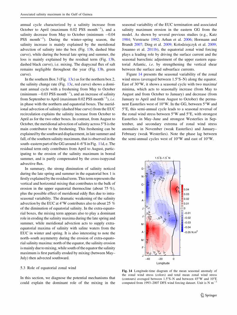
Figure 14 presents the seasonal variability of the zonal

wind stress (averaged between 1.5�S–N) along the equator.

East of 30�W, it shows a seasonal cycle with two maxima/

minima, which acts to seasonally increase (from May to

August and from October to January) and decrease (from

January to April and from August to October) the perma-

nent Easterlies west of 10�W. In the GG, between 5�W and

5�E, this semi-annual cycle leads to a seasonal reversal of

the zonal wind stress between 5�W and 5�E, with strongest

Easterlies in May–June and strongest Westerlies in Sep-

tember, and secondary extrema of zonal wind stress

anomalies in November (weak Easterlies) and January–

February (weak Westerlies). Note the phase lag between

the semi-annual cycles west of 10�W and east of 10�W.

−0.05 N.m2

−0.04

−0.03

−0.02

−0.01

0

0.01

0.02

0.03

0.04

0

00

−0.9

−0.8

−0.7

−0.7

−0.6

−0.6

−0.5

−0.5

−0.5

−0.4

−0.4

−0.4

−0.3

−0.3

−0.3

−0.3

−0.2

−0.2

−0.2

−0.

1

−0.1

−0.1

0.1

1.5°S−1.5° N

Longitude

−40 −20 0J

F

M

A

M

J

J

A

S

O

N

D

Fig. 14 Longitude-time diagram of the mean seasonal anomaly of

the zonal wind stress (colors) and total mean zonal wind stress

(contours) averaged between 1.5�S–N and between 45�W and 10�E

computed from 1993–2007 DFS wind forcing dataset. Unit is N m-2

Associated salinity maximum in the Gulf of Guinea

123

We now discuss the seasonal cycle of the EUC and its

associated saline waters in the light of the seasonal vari-

ability of the equatorial zonal wind and the surface cur-

rents. Figure 15 depicts the mean seasonal cycle for the

surface zonal currents and upper thermocline depth—

materialized by the rh = 26.2 isopycnal depth (first col-

umn; Fig. 15a, e, i), the vertically-averaged zonal veloci-

ties (second column; Fig. 15b, f, j) and salinity (third

column; Fig. 15c, g, k) in the upper thermocline, and the

vertical shear of zonal velocities computed from the sur-

face current and the upper thermocline vertically-averaged

velocities (last column; Fig. 15d, h, l).

At the equator, the semi-annual cycle of the zonal wind

stress forces a semi-annual cycle of the zonal current at the

surface, that manifests by a westward intensification in

boreal spring–summer and during November, and an

eastward reversal during early fall and winter (Fig. 15e;

color shading). The seasonal variability of the upper ther-

mocline depth anomalies also presents a semi-annual cycle

in quadrature (3-month phase lag) with the semi-annual

cycle of the surface current (Fig. 15e). This lag is charac-

teristic of the linear basin mode adjustment to the semi-

annual cycle of the equatorial wind stress described in

Cane and Moore (1981) or Ding et al. (2009). During the

late spring–summer and November–December periods, the

intensification of the surface currents and the shallowing of

the upper thermocline are concomitant with the erosion of

the EUC velocity and its associated salinity maximum

(Fig. 15f, g). Hence, as the surface current increases and

the thermocline heaves up, the vertical shear between the

EUC and the surface current is strongly enhanced at the

equator (Fig. 15h).

−0.2−0.1 0 0.1 0.2 0.3 0.4 0.5

U upper Th. (m.s−1)

(b)

35.7 35.8 35.9 36 36.1

Salinity (PSS)

(c)

−0.6 −0.4 −0.2 0 0.2 0.4 0.6

1.5° −

5° N

U Surf. (m.s−1)h

aσθ=26.2 (m)

(a)

JFMAMJJASOND

0 1 2 3 4 5 10−5

Shear2 (s−2)

(d)

(f) (g)

1.5° S

−1.

5° N

(e)

JFMAMJJASOND (h)

(j)

5W 0E 5E 10E

(k)

5W 0E 5E 10E

1.5° −

5° S

(i)

5W 0E 5E 10EJFMAMJJASOND (l)

5W 0E 5E 10E

Fig. 15 Longitude-time diagrams of mean seasonal cycle of (a) the

surface zonal velocities (in m s-1) and the seasonal anomaly of the

rh = 26.2 depth (in m; CI = 5 m; positive anomalies are in solid

line); b the EUC mean velocities in the upper thermocline (in m s-1);

c mean salinity in the upper thermocline (in PSS); and d the mean

vertical shear (in s-2) between the upper thermocline and the surface

averaged between 1.5�N–5�N. The white line at 4�W materializes the

western boundary of the boxes in Fig. 10. (e–h) same as (a–d), but

between 1.5�S–N. (i–l): same as (a–d), but between 5�s-1.5�S. The

dashed black lines represent the characteristics of the propagation

speed respectively for a Kelvin wave of the first (2.14 m s-1), second

(1.24 m s-1) and third (0.86 m s-1) baroclinic modes (e); and for

long Rossby waves of the first (0.71 m s-1), second (0.41 m s-1) and

third (0.29 m s-1) baroclinic modes (in a and i)

N. Kolodziejczyk et al.

123

North and south of the equator, the upper thermocline

depth anomalies (Fig. 15a, i) show a seasonal cycle asso-

ciated with a more marked annual component than at the

equator (Fig. 15e). In the southern hemisphere, the surface

zonal velocities exhibit a semi-annual cycle comparable

with those along the equator (Fig. 15e, i), while in the

northern part of the GG, the currents are mostly eastward

with a more marked annual cycle (Fig. 15a). The upper

thermocline depth anomalies exhibit a westward propaga-

tion visible in Fig. 15a and i, that is slower in the southern

hemisphere (between second and third baroclinic mode)

than in the northern hemisphere (less than the first baro-

clinic mode). In the upper thermocline layer, the currents

are westward on both sides of the EUC and exhibit a weak

variability (Fig. 15b, j), while the salinity experiences a

dominant annual cycle with a weakening from late spring

to winter (Fig. 15c, k). In the southern hemisphere, the

vertical shear of the zonal velocities is enhanced following

a semi-annual cycle that is in phase, though of lesser

amplitude, with the one at the equator (Fig. 15l, h). In

contrast, in the northern hemisphere, the vertical shear is

intensified during the westward intensification of the sur-

face currents during the late winter and summer (Fig. 15d).

At the equator, these diagnostics suggest that the salinity

maximum in the eastern GG is supplied by the EUC, and

that the salinity content and the EUC are subject to the

same seasonality. In the surface layer above the EUC, the

semi-annual cycle of the SEC is associated with the basin

adjustment of a second baroclinic basin mode to the semi-

annual cycle of the equatorial zonal wind (Ding et al.

2009). This adjustment manifests by the acceleration of the

SEC between 5�N–S due to the propagation of westward

Rossby waves from the eastern boundary of the GG, that

transport the saline water masses westward on the both

flanks of the EUC during the boreal late spring. The

adjustment is compatible with the propagation velocities

observed at the equator and in the southern hemisphere, but

not in the northern hemisphere. This discrepancy is prob-

ably due to the effects of the northern coast in the GG that

dramatically modifies the meridional structure of the

equatorial waves (Cane and Sarachik 1983). During the late

boreal spring and summer, the intensification of the west-

ward equatorial wind accelerates the SEC at the surface

and heaves the thermocline up at depth. The upper ther-

mocline is pinched off and the EUC saline water masses

are simultaneously eroded. It results that no more saline

waters can be advected in the eastern GG and recirculate in

the extra-equatorial branches. The decrease of EUC

transport, along with the erosion of its associated salinity

maximum, can thus be explained by the vertical mixing

induced by the stronger vertical shear between the surface

and upper thermocline currents during boreal spring and

fall, in agreement with results by Jouanno et al. (2011b).

6 Discussion and conclusion

This paper describes in a first part the time evolution of

EUC water masses during boreal summer in the eastern

equatorial Atlantic from a new set of in situ observations

including both currents and salinity measurements. It pro-

vides strong observational evidence of the existence of an

intense seasonal variability of the circulation and salinity in

the upper thermocline in the GG from boreal late spring to

fall. The more striking signature of this variability is the

presence of westward extra-equatorial recirculations of

EUC water masses in late boreal spring (early summer) and

the absence of a direct supply of EUC saline water masses

from the west in mid and late summer. This is due to (i) the

progressive weakening of the upper thermocline EUC in

the GG in boreal summer, and (ii) the concomitant erosion

of the salinity maximum west of the GG induced by the

outcropping of the thermocline in the mixed layer (Voitu-

riez 1983; Verstraete 1992) and/or by enhanced vertical

diffusion in the surface layer (Gouriou and Reverdin 1992;

Jouanno et al. 2011a). All seven cruises and Argo obser-

vations used in this study support this seasonal cycle. Some

observed differences between repeated sections however

suggest some inter-annual and/or intra-seasonal variability

(Marin et al. 2009).

In situ cruises observations used in this study were mostly

collected between June and November, thus preventing us

from analyzing the complete seasonal cycle of the upper

thermocline circulation. Therefore, in order to study the

complete seasonal variability of the termination of the EUC

and the fate of associated saline waters in the GG, we used

validated NEMO model outputs from 1993 to 2007 and

compared them with the repeated cruises sections, as previ-

ously done at 10�W by Kolodziejczyk et al. (2009).

Simulations of the upper layers of the eastern equatorial

Atlantic Ocean are known to be strongly sensitive to the

parameterization of the vertical mixing (Pacanowski and

Philander 1981; Wacongne 1989; Blanke and Delecluse

1993). Considering the high sensitivity of the EUC prop-

erties to the vertical viscosity in the models (Boning and

Kroger 2005), vertical mixing is suspected to be respon-

sible for the bias in salinity observed in the upper ther-

mocline in the model, and the discrepancy of the

stratification and EUC strength reported in the model val-

idation section. However, in boreal summer the model is

qualitatively consistent with the variability observed in our

data set but also in several previous observations in the

region (Hisard and Morliere 1973; Verstraete 1992; Gou-

riou and Reverdin 1992; Mercier et al. 2003; Bourles et al.

2002), thus confirming the seasonal cycle suggested by the

sparse observations.

The analysis of the mean seasonal variability of the

upper thermocline has established a robust seasonal cycle.

Associated salinity maximum in the Gulf of Guinea

123

The model allowed us to quantify the seasonal salinity

budget in the upper thermocline in the eastern GG. It

appears first that the amount of saline waters in the upper

thermocline of the GG is strongly dependent of the upper

EUC transport that contributes to feed the eastern GG and

extra-equatorial salinity maxima, mainly during the boreal

spring. Such a feature is consistent with the earlier obser-

vations made in 1995 by Mercier et al. (2003). A direct

poleward recirculation of the EUC water masses along the

African Coast in the coastal GCUC was suggested by

Wacongne and Piton (1992). Our observations do not allow

to sample the GCUC which remains poorly documented in

the literature (Wacongne and Piton 1992). The existence of

such an along-coast EUC continuation is also suggested in

the model. However, it only exports about 0.2 ± 0.6 Sv of

upper thermocline water masses southward, which repre-

sents only a very small part of the EUC transport.

From May to September, the upper EUC transport in the

west of the GG is minimum in the model and advects no

more saline water masses into the GG, as suggested by

previous observations (Gouriou and Reverdin 1992; Kol-

odziejczyk et al. 2009). West of 10�W, Jouanno et al.

(2011a, b, 2013) demonstrated that the enhancement of

vertical mixing during this season strongly contributes to

the cooling of the subsurface temperature at the upper

bound of the EUC. In the GG, Da-Allada et al. (2014) have

recently shown from a numerical study an increase of the

mixed layer salinity during boreal late spring and summer.

This increase results from the dominance of the vertical

diffusion of subsurface saline waters over they freshwater

surface advection originating from river run off in the

eastern GG during this period. Our study suggests that the

intensified vertical mixing also contributes to erode the

upper EUC and its salinity maximum not only west of

10�W, thus explaining the reduction of the saline waters

advected in the eastern GG, but also in the GG between 4�S

and 4�N to locally entrain waters from the upper EUC into

the surface mixed layer. The vertical mixing may contribute

to the progressive erosion of the equatorial and extra-

equatorial maxima of salinity during boreal summer, in

agreement with the enhancement of our residual term of

salinity (loss) during this season. However, in the GG, the

local vertical mixing may be not the unique mechanism

responsible for the seasonal erosion of salinity, and our

results indeed indicate that the contribution of horizontal

advection to the seasonal cycle is also important, in par-

ticular during the second part of the year (Fig. 12). Though

the vertical mixing is not as strong in the eastern as in the

western GG, it remains a dominant contributor to the mixed

layer heat budget (Jouanno et al. 2011a, b; Da-Allada et al.

2014, Berger et al. 2014) and to the upper salinity budget

(Da-Allada et al. 2013). In the GG, the contribution of

vertical mixing to the salinity budget in the eastern GG can

also be distant, through the advection of less saline waters

that have been previously freshened through turbulent

vertical mixing by surface waters in the west (between

20�W and 0�E). In the easternmost part of the GG, the

strong surface desalinization due to the rivers’ runoff is

likely to also play a significant role in the dynamical and

salinity balance of the upper GG (Hisard 1973; Jouanno

et al. 2011a; Da-Allada et al. 2013). Following model

results from Berger et al. (2014), the lateral mixing and

eddy diffusivity could also play a significant role in eroding

the EUC and extra-equatorial salinity maximum. Finally,

some intra-seasonal features like the 15-day variability

observed near the equator in the GG (Athie and Marin 2008;

de Coetlogon et al. 2010; Jouanno et al. 2013), could con-

tribute to the erosion of salt during boreal summer.

From boreal fall to winter, the EUC appears to reinforce

in the upper thermocline, bringing back saline water mas-

ses into the eastern GG, which progressively spreads along

the coast in the equatorial band and supplies again the

extra-equatorial salinity maxima. During December–Janu-

ary, the salinity and upper thermocline are slightly eroded.

This is reminiscent to the reinforcement of the surface

current and of the second weaker upwelling that is present

from November to January in the central and eastern

equatorial Atlantic, as suggested by Arhan et al. (2006),

Okumura and Xie (2006), Ding et al. (2009) or Jouanno

et al. (2011a).

Ding et al. (2009) have studied the seasonal cycle of the

sea surface height (SSH) and surface currents in equatorial

Atlantic. They have shown that the thermocline and surface

currents adjust to the semi-annual cycle of the zonal wind

over the Atlantic basin. The reinforcement of the wind

during boreal spring and fall induces the semi-annual

intensification of the surface currents and of the thermo-

cline upwelling in the GG that is in return enhanced by a

semi-annual basin mode. Some other studies (e.g.,

Houghton 1983; Hormann and Brandt 2007; Ding et al.

2009) have linked the seasonal variability in the upper

ocean in the GG to a basin scale adjustment to the seasonal

variations in easterlies. This equatorial adjustment mani-

fests in late boreal spring by the propagation of an

upwelling Kelvin wave that reflects into equatorial Rossby

waves at the African coast (Philander 1986; Ding et al.

2009). The semi-annual reinforcement of the surface cur-

rents plays a key role in the enhancement of turbulent

mixing that erodes the upper EUC in the central Atlantic

(Jouanno et al. 2011a).

An important aspect of the variability of the termination

of the EUC in the GG is the fate of its saline water masses

of subtropical origin involved in the larger meridional

circulation of STC and TC (e.g., Blanke et al. 2002;

Snowden and Molinari 2003; Zhang et al. 2003; Hazeleger

and De Vries 2003; Molinari et al. 2003; Wang 2005). The

N. Kolodziejczyk et al.

123

seasonal variability of the EUC termination and associated

salinity maximum inferred from both the observations and

the model reveals slightly different features than the STC

mean circulation picture. During the first part of the year,

the EUC water masses rather appears to join the eastern

boundary of the equatorial Atlantic and to recirculate off

the equator within the upper thermocline, without any

contact with the surface. During boreal spring and summer,

and November–December, the erosion of the upper EUC

termination and saline waters is strongly associated with

the upwelling intensity through vertical advection and

mixing. The exact contribution of this seasonal cycle for

the mean view of the STC would require further analysis.

Acknowledgments Based on a French initiative, AMMA was built

by an international scientific group and was funded by a large number

of agencies, from France, UK, US and Africa. It benefited of a major

financial contribution from the European Community’s Sixth

Framework Research Programme. Refer to: http://www.amma-inter

national.org for detailed information on this program. The authors

also thank the PIRATA program for providing for free precious data

sets to the whole scientific community. Authors do thank Jacques

Grelet, Fabrice Roubaud, Remy Chuchla and vessels’ crews who

make possible the in situ data acquisition during all EGEE/AMMA

and yearly PIRATA cruises. The Argo data are validated and kindly

provided by Fabienne Gaillard (LPO, CNRS/Ifremer/IRD/UBO,

Brest, France), and funded by the CNES-TOSCA project ‘GLO-

SCAL’. Authors do also thank Anne-Marie Treguier for valuable

discussions on NEMO simulations, and anonymous reviewers for

constructive remarks that helped to substantially improve the

manuscript.

References

Antonov JI, Seidov D, Boyer TP, Locarnini RA, Mishonov AV,

Garcia HE, Baranova OK, Zweng MM, Johnson DR (2010)

World ocean atlas 2009, volume 2: salinity. In: Levitus S (ed)

NOAA atlas NESDIS 69, U.S. Government Printing Office,

Washington, DC, 184 pp

Arhan M, Treguier AM, Bourles B, Michel S (2006) Diagnosing the

annual cycle of the equatorial undercurrent in the Atlantic Ocean

from a general circulation model. J Phys Oceanogr

36:1502–1522

Athie G, Marin F (2008) Cross-equatorial structure and temporal

modulation of intraseasonal variability at the surface of the

Tropical Atlantic Ocean. J Geophys Res 113:C08020. doi:10.

1029/2007JC004332

Barnier B, Marchesiello P, de Miranda AP, Molines JM, Coulibaly M

(1998) A sigma-coordinate primitive equation model for study-

ing the circulation in the South Atlantic. Part I: model

configuration with error estimates. Deep Sea Res 45:543–572

Barnier B, Madec G, Penduff T, Molines J-M, Treguier A-M, Le

Sommer J, Beckmann A, Biastoch A, Boning C, Dengg J, Derval

C, Durand E, Gulev S, Remy E, Talandier C, Theetten S,

Maltrud M, McClean J, De Cuevas B (2006) Impact of partial

steps and momentum advection schemes in a global ocean

circulation model at eddy permitting resolution. Ocean Dyn 4.

doi:10.1007/s10236-006-0082-1

Berger H, Treguier A-M, Perenne N, Talandier C (2014) Dynamical

contribution to sea surface salinity variations in the eastern Gulf

of Guinea base on numerical modelling. Clim Dyn (submitted)

Blanke B, Delecluse P (1993) Variability of the tropical Atlantic

Ocean simulated by a general circulation model with two

different mixed-layer physics. J Phys Oceanogr 23:1363–1388

Blanke B, Arhan M, Lazar A, Prevost G (2002) A Lagrangian

numerical investigation of the origins and fates of the salinity

maximum water in the Atlantic. J Geophys Res 107(C10):3163.

doi:10.1029/2002JC001318

Boning CW, Kroger J (2005) Seasonal variability of deep currents in

the equatorial Atlantic: a model study. Deep Sea Res I

52:99–121

Bourles B, Gouriou Y, Chuchla R (1999) On the circulation in the

upper layer of the western equatorial Atlantic. J Geophys Res

104:21151–21170

Bourles B, D’Orgeville M, Eldin G, Gouriou Y, Chuchla R, du

Penhoat Y, Arnault S (2002), On the evolution of the thermo-

cline and subthermocline eastward currents in the equatorial

Atlantic. Geophys Res Lett 29. doi:10.1029/2002GL015098

Bourles B, Brandt P, Caniaux G, Dengler M, Gouriou Y, Key E,

Lumpkin R, Marin F, Molinari RL, Schmid C (2007) African

monsoon multidisciplinary analysis (AMMA): special measure-

ments in the tropical Atlantic. CLIVAR Exch Lett 41(12):2

Bourles B, Lumpkin R, McPhaden MJ, Hernandez F, Nobre P,

Campos E, Yu L, Planton S, Busalacchi A, Moura AD, Servain J,

Trotte J (2008) The PIRATA program: history, accomplishments

and future directions. Bull Am Meteorol Soc 89:1111–1125

Brandt P, Schott FA, Provost C, Kartavtseff A, Hormann V, Bourles

B, Fischer J (2006) Circulation in the central equatorial Atlantic:

mean and intraseasonal to seasonal variability. Geophys Res Lett

33:L07609. doi:10.1029/2005GL025498

Brodeau L, Barnier B, Treguier A-M, Penduff T, Gulev S (2010) An

ERA-40-based atmospheric forcing for global ocean circulation

models. Ocean Model 31:88–104

Cane MA, Moore DW (1981) A note on low-frequency equatorial

basin modes. J Phys Oceanogr 11:1578–1584

Cane MA, Sarachik ES (1983) Equatorial oceanography. Rev

Geophys 21:1137–1148

Chang P, Zhang R, Hazeleger W, Wen C, Wan X, Ji L, Haarsma RJ,

Breugem W-P, Seidel H (2008) Oceanic link between abrupt

changes in the north Atlantic Ocean and the African monsoon.

Nature 1:444–448

Da-Allada CY, Alory G, du Penhoat Y, Kestenare E, Durand F,

Hounkonnou NM (2013) Seasonal mixed-layer salinity balance

in the tropical Atlantic Ocean: mean state and seasonal cycle.

J Geophys Res 118:332–345. doi:10.1029/2012JC008357

Da-Allada CY, du Penhoat Y, Jouanno J, Allory G, Hounkonnou NM

(2014) Mixed layer salinity balance in the Gulf of Guinea:

seasonal and interannual variability. Clim Dyn (submitted)

Dai A, Trenberth KE (2002) Estimates of freshwater discharge from

continents: latitudinal and seasonal variations. J Hydrometeorol

3:660–687

de Coetlogon G, Janicot S, Lazar A (2010) Intra-seasonal variability

of the ocean-atmosphere coupling in the Gulf of Guinea during

boreal spring and summer. Q J Roy Meteorol Soc 136:426–441

Ding H, Keenlyside NS, Latif M (2009) Seasonal cycle in the upper

equatorial Atlantic Ocean. J Geophys Res 114:C09016. doi:10.

1029/2009JC005418

Gaillard F, Autret E, Thierry V, Galaup P, Coatanoan C, Loubrieu T

(2009) Quality control of large Argo data sets. J Atmos Ocean

Technol 26(2):337–351

Giarolla E, Nobre P, Malagutti M, Pezzi LP (2005) The Atlantic

equatorial undercurrent: PIRATA observations and simulations

with GFDL modular ocean model at CPTEC. Geophys Res Let

32. doi:10.1029/2004GL022206

Gouriou Y, Reverdin G (1992) Isopycnal and diapycnal circulation of

the upper equatorial Atlantic Ocean in 1983–1984. J Geophys

Res 97:3543–3572

Associated salinity maximum in the Gulf of Guinea

123

Grodsky SA, Carton JA (2002) Surface drifter pathways originating in

the equatorial Atlantic cold tongue. Geophys Res Lett 29:2147.

doi:10.1029/2002GL015788

Han W, Webster PJ, Lin J-L, Liu WT, Fu R, Yuan D, Hu A (2008)

Dynamics of intraseasonal sea level and thermocline variability

in the equatorial Atlantic during 2002–03. J Phys Oceanogr

38:945–966

Hazeleger W, de Vries P (2003) Fate of the equatorial undercurrent in

the Atlantic. In Goni GJ, Malanotte-Rizzoli P (eds) Interhemi-

spheric water exchange in the Atlantic ocean. Amsterdam,

Elsevier, pp 175–191

Hazeleger W, de Vries P, Friocourt Y (2003) Sources of the

equatorial undercurrent in the Atlantic in a high-resolution ocean

model. J Phys Oceanogr 33:677–693

Hisard P (1973) Variations saisonnieres a l’equateur dans le Golfe de

Guinee, Cah. ORSTOM Ser Oceanogr XI: 349–358

Hisard P, Morliere A (1973), La terminaison du contre-courant

equatorial subsuperficiel atlantique (courant de Lomonosov) dans

le Golfe de Guinee, Cah. ORSTOM, Ser Oceanogr XI:455–464

Hormann V, Brandt P (2007) Atlantic Equatorial Undercurrent and

associated cold tongue variability. J Geophys Res 112:C06017.

doi:10.1029/2006JC003931

Houghton RW (1983) Seasonal variations of the subsurface thermal

structure in the Gulf of Guinea. J Phys Oceanogr 13:2070–2081

Hummels R, Dengler M, Bourles B (2013) Seasonal and regional

variability of upper ocean diapycnal heat flux in the Atlantic

Cold Tongue. Prog Oceanogr 111:52–74

Johns WE, Brandt P, Bourles B, Tantet A, Papapostolou A, Houk A

(2014) Zonal structure and seasonal variability of the atlantic

equatorial undercurrent. Clim Dyn (submitted)

Jouanno J, Marin F, du Penhoat Y, Sheinbaum J, Molines JM (2011a)

Seasonal heat balance in the upper 100 m of the Equatorial

Atlantic Ocean. J Geophys Res 116:C09003. doi:10.1029/

2010JC006912

Jouanno J, Marin F, du Penhoat Y, Molines JM, Sheinbaum J (2011b)

Seasonal modes of surface cooling in the Gulf of Guinea. J Phys

Oceanogr 41:1408–1416. doi:10.1175/JPO-D-11-031.1

Jouanno J, Marin F, du Penhoat Y, Molines JM (2013) Intraseasonal

modulation of the surface cooling in the Gulf of Guinea. J Phys

Oceanogr 43:382–401. doi:10.1175/JPO-D-12-053.1

Katz E (1984) Basin wide thermocline displacements along the

equator of the Atlantic in 1983. Geophys Res Lett 11:729–732.

doi:10.1029/GL011i008p00729

Katz E, Molinari RL, Cartwright D, Hisard P, Lass H, deMesquita A

(1981) The seasonal transport of the Equatorial Undercurrent in

the western Atlantic (during the Global Weather Experiment).

Ocean Acta 4:445–450

Kolodziejczyk N, Bourles B, Marin F, Grelet J, Chuchla R (2009)

Seasonal variability of the equatorial undercurrent at 10 W as

inferred from recent in situ observations. J Geophys Res

114:C06014. doi:10.1029/2008JC004976

Locarnini RA, Mishonov AV, Antonov JI, Boyer TP, Garcia HE,

Baranova OK, Zweng MM, Johnson DR (2010) World Ocean

Atlas 2009, Volume 1: Temperature. In: S. Levitus (ed) NOAA

Atlas NESDIS 68, U.S. Government Printing Office, Washing-

ton, DC, 184 pp

Lumpkin R, Speer K (2003) Large-scale vertical and horizontal

circulation in the North Atlantic Ocean. J Phys Oceanogr

33:1902–1920. doi:10.1175/1520-0485(2003)033\1902:LVAHC

I[2.0.CO;2

Madec G (2008) NEMO ocean engine: version3.1, Note du Pole de

modelisation de l’IPSL n�27

Marin F, Caniaux G, Giordani H, Bourles B, Gouriou Y, Key E

(2009) Why were sea surface temperatures so different in the

eastern equatorial Atlantic in June 2005 and 2006? J Phys

Oceanogr 39:1416–1431

Mercier H, Arhan M, Lutjeharms J (2003) Upper-layer circulation in

the eastern equatorial and South Atlantic Ocean in January–

March 1995. Deep Sea Res I 50:863–887

Molinari RL, Bauer S, Johnson GC, Bourles B, Gouriou Y, Mercier H

(2003) A comparison of kinematic evidence for tropical cells in

the Atlantic and Pacific oceans. In: Goni GJ, Malanotte-Rizzoli P

(eds) Interhemispheric water exchange in the Atlantic Ocean.

Elsevier, Amsterdam

Okumura Y, Xie S-P (2006) Some overlooked features of Tropical

Atlantic climate leading to a new Nino-like Phenomenon. J Clim

19:5859–5874

Pacanowski RC, Philander SGH (1981) Parameterization of vertical

mixing in numerical models of Tropicals Oceans. J Phys

Oceanogr 11:1443–1451

Peter A-C, Le Henaff M, du Penhoat Y, Menkes CE, Marin F, Vialard

J, Caniaux G, Lazar A (2006) A model study of the seasonal

mixed layer heat budget in the equatorial Atlantic. J Geophys

Res 111:C06014. doi:10.1029/2005JC003157

Philander SGH, Pacanowski R (1986) A model of the seasonal cycle

of the Tropical Atlantic ocean. J Geophys Res 91:14192–14206

Redelsperger J-L, Thorncroft CD, Diedhiou A, Lebel T, Parker DJ,

Polcher J (2006) African monsoon multidisciplinary analysis: an

international research project and field campaign. Bull Am

Meteorol Soc 87:1739–1746

Rhein M, Dengler M, Sultenfuß J, Hummels R, Huttl-Kabus S,

Bourles B (2010) Upwelling and associated heat flux in the

equatorial Atlantic inferred from helium isotope disequilibrium.

J Geophys Res 115:C08021. doi:10.1029/2009JC005772

Richardson P, Reverdin G (1987) Seasonal cycle of velocity in the

Atlantic NECC as measured by surface drifters, current meters

and ship drifts. J Geophys Res 92:3691–3708

Schott FA, Fischer J, Stramma L (1998) Transports and pathways of

the upper-layer circulation in the western tropical Atlantic.

J Phys Oceanogr 28:1904–1928

Snowden D, Molinari RL (2003), Subtropical cells in the Atlantic

ocean: an observational summary. In: Goni GJ, Malanotte-

Rizzoli P (eds) Interhemispheric water exchange in the Atlantic

Ocean. Elsevier Oceanography Series 68:287–312

Stramma L, Schott F (1999) The mean flow field of the tropical

Atlantic Ocean. Deep Sea Res II 46(1–2):279–303

Treguier A-M, Barnier B, De Miranda AP, Molines JM, Grima N, Imbard

N, Madec G, Messager C (2001) Eddy permitting model of the

Atlanticcirculation:evaluatingopenboundaryconditions. JGeophys

Res 106(C10):22115–22129. doi:10.1029/2000JC000376

Verstraete J-M (1992) The seasonal upwellings in the Gulf of Guinea.

Prog Oceanogr 29:1–60

Voituriez B (1983) Les variations saisonnieres des courants equator-

iaux a 4�W et l’upwelling equatorial du Golfe de Guinee, I. Le

sous-courant equatorial. Oceanogr Trop 18(2): 163–183

Wacongne S (1989) Dynamical regimes of fully nonlinear stratified

model of the Atlantic Equatorial Undercurrent. J Geophys Res

94(C4):4801–4815

Wacongne S, Piton B (1992) The near-surface circulation in the

northeastern corner of the South Atlantic Ocean. Deep-Sea Res

39:1273–1298

Wade M, Caniaux G, du Penhoat Y (2011) Variability of the mixed

layer heat budget in the eastern equatorial Atlantic during

2005–2007 as inferred using Argo floats. J Geophys Res

116:C08006. doi:10.1029/2010JC006683

Wang C (2005) Subthermocline tropical cells and equatorial subsur-

face countercurrents. Deep-Sea Res I 52:123–135

Zhang D, McPhaden MJ, Johns WE (2003) Observational evidence

for flow between the subtropical and tropical Atlantic: the

Atlantic subtropical cells. J Phys Oceanogr 33:1783–1797

N. Kolodziejczyk et al.

123