Seasonal changes in Fe species and soluble Fe ... · fate and oxalate originated from anthropogenic sources, ... joint project, ... pling with a reading precision of 10µg after stabilizing

Atmos. Chem. Phys., 13, 7695–7710, 2013www.atmos-chem-phys.net/13/7695/2013/doi:10.5194/acp-13-7695-2013© Author(s) 2013. CC Attribution 3.0 License.

EGU Journal Logos (RGB)

Advances in Geosciences

Open A

ccess

Natural Hazards and Earth System

Sciences

Open A

ccess

Annales Geophysicae

Open A

ccessNonlinear Processes

in Geophysics

Open A

ccess

Atmospheric Chemistry

and PhysicsO

pen Access

Atmospheric Chemistry

and Physics

Open A

ccess

Discussions

Atmospheric Measurement

Techniques

Open A

ccess

Atmospheric Measurement

Techniques

Open A

ccess

Discussions

Biogeosciences

Open A

ccess

Open A

ccess

BiogeosciencesDiscussions

Climate of the Past

Open A

ccess

Open A

ccess

Climate of the Past

Discussions

Earth System Dynamics

Open A

ccess

Open A

ccess

Earth System Dynamics

Discussions

GeoscientificInstrumentation

Methods andData Systems

Open A

ccess

GeoscientificInstrumentation

Methods andData Systems

Open A

ccess

Discussions

GeoscientificModel Development

Open A

ccess

Open A

ccess

GeoscientificModel Development

Discussions

Hydrology and Earth System

Sciences

Open A

ccess

Hydrology and Earth System

Sciences

Open A

ccess

Discussions

Ocean Science

Open A

ccess

Open A

ccess

Ocean ScienceDiscussions

Solid Earth

Open A

ccess

Open A

ccess

Solid EarthDiscussions

The Cryosphere

Open A

ccess

Open A

ccess

The CryosphereDiscussions

Natural Hazards and Earth System

Sciences

Open A

ccess

Discussions

Seasonal changes in Fe species and soluble Fe concentration in theatmosphere in the Northwest Pacific region based on the analysis ofaerosols collected in Tsukuba, Japan

Y. Takahashi1,2,3,*, T. Furukawa1, Y. Kanai4, M. Uematsu2, G. Zheng3, and M. A. Marcus5

1Department of Earth and Planetary Systems Science, Graduate School of Science, Hiroshima University, Higashi-Hiroshima,Hiroshima 739-8526, Japan2Atmosphere and Ocean Research Institute, The University of Tokyo, 5-1-5 Kashiwanoha, Kashiwa, Chiba 277-8564, Japan3Key Laboratory of Petroleum Resources, Chinese Academy of Sciences, 382 Donggang Road, Lanzhou 730000, China4Geological Survey of Japan, National Institute of Advanced Industrial Science and Technology (AIST), 1-1-1 Higashi,Tsukuba, Ibaraki 305-8567, Japan5Advanced Light Source, Lawrence Berkeley National Laboratory, Berkeley, CA 94720, USA

Correspondence to:Y. Takahashi ([email protected])

Received: 21 January 2013 – Published in Atmos. Chem. Phys. Discuss.: 20 March 2013Revised: 26 June 2013 – Accepted: 28 June 2013 – Published: 9 August 2013

Abstract. Atmospheric iron (Fe) can be a significant sourceof nutrition for phytoplankton inhabiting remote oceans,which in turn has a large influence on the Earth’s climate.The bioavailability of Fe in aerosols depends mainly on thefraction of soluble Fe (= [FeSol]/[FeTotal], where [FeSol] and[FeTotal] are the atmospheric concentrations of soluble andtotal Fe, respectively). However, the numerous factors affect-ing the soluble Fe fraction have not been fully understood. Inthis study, the Fe species, chemical composition, and solu-ble Fe concentrations in aerosols collected in Tsukuba, Japanwere investigated over a year (nine samples from Decem-ber 2002 to October 2003) to identify the factors affectingthe amount of soluble Fe supplied into the ocean. The solubleFe concentration in aerosols is correlated with those of sul-fate and oxalate originated from anthropogenic sources, sug-gesting that soluble Fe is mainly derived from anthropogenicsources. Moreover, the soluble Fe concentration is also cor-related with the enrichment factors of vanadium and nickelemitted by fossil fuel combustion. These results suggest thatthe degree of Fe dissolution is influenced by the magnitudeof anthropogenic activity, such as fossil fuel combustion.

X-ray absorption fine structure (XAFS) spectroscopy wasperformed in order to identify the Fe species in aerosols. Fit-ting of XAFS spectra coupled with micro X-ray fluorescenceanalysis (µ-XRF) showed the main Fe species in aerosols

in Tsukuba to be illite, ferrihydrite, hornblende, and Fe(III)sulfate. Moreover, the soluble Fe fraction in each samplemeasured by leaching experiments is closely correlated withthe Fe(III) sulfate fraction determined by the XAFS spec-trum fitting, suggesting that Fe(III) sulfate is the main solu-ble Fe in the ocean. Another possible factor that can controlthe amount of soluble Fe supplied into the ocean is the to-tal Fe(III) concentration in the atmosphere, which was highin spring due to the high mineral dust concentrations duringspring in East Asia. However, this factor does not contributeto the amount of soluble Fe to a larger degree than the ef-fect of Fe speciation, or more strictly speaking the presenceof Fe(III) sulfate. Therefore, based on these results, the mostsignificant factor influencing the amount of soluble Fe in theNorth Pacific region is the concentration of anthropogenicFe species such as Fe(III) sulfate that can be emitted frommegacities in Eastern Asia.

1 Introduction

Oceanic areas where phytoplankton growth is limited by iron(Fe) concentration are called “high nutrient, low chlorophyll(HNLC)” regions (Martin and Fitzwater, 1988), which ac-count for 20 % to 30 % of the world’s oceans (Martin, 1990;

Published by Copernicus Publications on behalf of the European Geosciences Union.

7696 Y. Takahashi et al.: Seasonal changes in Fe species and soluble Fe concentration

Jickells et al., 2005; Boyd and Ellwood, 2010). The con-centration of bioavailable Fe in the euphotic zone in theocean can influence the photosynthesis of phytoplankton inthe HNLC, which can consequently affect the carbon cycleon the Earth’s surface. Moreover, the amount of Fe in remoteoceans can increase the production of dimethyl sulfide and/ororganic carbon from microorganisms in the ocean, which inturn affects the radiative forcing in the atmosphere (Bishopet al., 2002; Boyd et al., 2007). Thus, understanding the pro-cesses of Fe supply and dissolution Fe from the atmosphereinto the ocean is essential in estimating the impact of Fe onthe Earth’s climate.

Previous studies have demonstrated that several sources ofFe, such as (1) atmospheric particles (Duce et al., 1991),(2) the continental shelf (Lam and Bishop, 2008), (3) is-lands in the ocean (Martinez and Maamaatuaiahutapu, 2004),(4) volcanic dust (Langmann et al., 2010), and (5) shipboardaerosol sources (Ito et al., 2013) provide significant solubleFe to phytoplankton inhabiting remote oceans. Among theseFe sources, Fe in aerosols can be an important fraction (Duceet al., 1991; Jickells and Spokes, 2001). Therefore, severalprevious studies have investigated the soluble Fe concentra-tion in the atmosphere to understand the influence of airborneFe on the Earth’s surface environment (e.g. Baker and Jick-ells, 2006; Buck et al., 2010; Sedwick et al., 2007; Aguilar-Islas et al., 2010).

However, the factors controlling soluble Fe fractions inaerosols have not been understood fully because a numberof factors are involved (Mahowald et al., 2005). Thus, the at-mospheric concentrations of total Fe ([FeTotal]) and solubleFe ([FeSol]), both in ng m−3 need to be distinguished fromsoluble Fe fractions (fsol = [FeSol]/[FeTotal]) in the aerosols.For example, the soluble Fe fraction is influenced by thesource(s) (Sedwick et al., 2007; Aguilar-Islas et al., 2010;Paris et al., 2010), aerosol size (Baker and Jickells, 2006;Ooki et al., 2009), and mineralogy (Journet et al., 2008) ofthe aerosols, as well as heterogeneous reactions with acidsin the atmosphere (Spokes and Jickells, 1996; Mackie et al.,2005; Shi et al., 2009).

The atmospheric concentration of soluble Fe (= [FeSol]),which is important in understanding the amount of bioavail-able Fe to the ocean, is the product of [FeTotal] and the solubleFe fraction (= fsol): [FeSol] = fsol× [FeTotal]. Here, [FeTotal]should also be important to consider [FeSol], which can beincreased during spring in the North Pacific region due to thesupply of mineral dust from China. On the other hand, somereports have suggested that Fe from anthropogenic sourcesis highly soluble, therefore can be a significant source ofbioavailable Fe dissolved in the ocean (Sedwick et al., 2007;Luo et al., 2008; Schroth et al., 2009; Sholkovitz et al., 2009;Kumar and Sarin, 2010).

In this study, we used X-ray absorption fine structure(XAFS), which is a powerful analytical tool to identify chem-ical species of Fe and other elements in aerosols to spe-ciate Fe in aerosols (Majestic et al., 2007; Schroth et al.,

2009; Takahashi et al., 2011; Oakes et al., 2012a, b; Fu-rukawa and Takahashi, 2011). Identifying the Fe speciesin aerosols can improve understanding of the factors con-trolling [FeSol]/[FeTotal], because this ratio is strongly re-lated to the Fe species. XAFS consists of X-ray absorptionnear edge structure (XANES) and extended X-ray absorp-tion fine structure (EXAFS) which can determine the chem-ical species of each element in aerosols. We also conductedleaching experiments with two leaching solutions to studythe relationship between the [FeSol]/[FeTotal] ratio and Fespecies. By combining atmospheric Fe concentration, XAFSanalysis, and leaching experiments, we revealed importantfactors controlling the supply of soluble Fe into the ocean.

Aerosol samples used in this study were collected throughone year (nine samples collected at different months fromDecember 2002 to October 2003; Table 1) in Tsukuba, 60 kmnortheast from Tokyo, Japan, at 36.06◦ N, 140.14◦ E. Al-though the sampling period does not cover the whole yearround, the collection of the sample from December 2002to October 2003 can give us an idea of variation of [FeSol]and [FeTotal] in the atmosphere. Tsukuba is a site suitable forcharacterizing aerosols that can be transported to the North-west Pacific by westerlies. The various sources of aerosolsin Tsukuba include (i) mineral dust from the continent,(ii) anthropogenic aerosols from megacities and industrialareas around Tokyo and from the continent, and (iii) ma-rine aerosols from the Pacific Ocean. Considering these threesources vary depending on the season, determining the sea-sonal variations in the contribution of each factor to the Fespeciation in aerosols related to the [FeSol]/[FeTotal] is im-portant.

2 Materials and methods

2.1 Aerosol samples and characterization

The total suspended particles (TSP) in the atmosphere weredetermined in this study using a high-volume air sampler(Sibata, HV-1000F, Tokyo, Japan) at Tsukuba (Latitude:36.06◦ N, Longtitude: 140.14◦ E, Height: 44 m a.s.l.) fromDecember 2002 to October 2003 as part of the Japan–Chinajoint project, “Asian Dust Experiment on Climate Impact”(Kanai et al., 2003; Table 1). This method can collect drydeposition or total suspended particles (TSP) in the atmo-sphere, whereas wet deposition samples were not collectedin this study. The flow rate of the air sampler during sam-pling was maintained at 1000 L min−1, and polyflon filters(25 cm× 20 cm; Advantec, PF40) were used for collectingaerosols. The filters were weighed before and after sam-pling with a reading precision of 10 µg after stabilizing theweight under constant humidity in a desiccator. The filterswith aerosols were preserved in a desiccator to prevent thechemical change of Fe in the aqueous phase at aerosol sur-faces. Three-dimensional air mass back trajectories were

Atmos. Chem. Phys., 13, 7695–7710, 2013 www.atmos-chem-phys.net/13/7695/2013/

Y. Takahashi et al.: Seasonal changes in Fe species and soluble Fe concentration 7697

Table 1. Periods for the collection of the TSP samples used in this study.

Start Stop TSP Total precipitation Number of rain eventsconcentration during the period (total precipitation> 5 mm)

(mg m−3) (mm)a during the perioda

December 17.12.2002 08.01.2003 29.25 50 2 (3 daysb)February 13.02.2003 24.02.2003 42.55 27 2 (2 days)March 14.03.2003 25.03.2003 41.41 8.5 2 (3 days)May 01.05.2003 12.05.2003 54.26 17.5 1 (1 day)June 11.06.2003 20.06.2003 36.55 12.5 1 (2 days)July 11.07.2003 22.07.2003 29.39 56.5 3 (4 days)August 12.08.2003 21.08.2003 14.54 199 2 (3 days)September 22.09.2003 30.09.2003 20.84 19 1 (2 days)October 10.10.2003 21.10.2003 28.17 77.5 1 (2 days)

a Data from website of Japan Meteorological Agency (http://www.jma.go.jp/jma/index.html), b Number of days covered by the rain eventsduring the period.

calculated at a height of 1000 m using the Hybrid Single-Particle Lagrangian-Integrated Trajectory model (Draxlerand Rolph, 2003).

Aerosols on the filter were digested with a mineral acidmixture (30 % HCl+ 68 % HNO3+ 38 % HF) at 160◦C for6 h, after which the acids were evaporated to near drynessat 140◦C to determine the total chemical compositions. Theresidue was dissolved in 2 % HNO3, and the total concen-trations of Na, Mg, Al, Ca, Mn, Fe, Cu, Zn, and Pb inthe aerosols were determined by inductively coupled plasmaatomic emission microscopy (ICP-AES; SII NanoTechnol-ogy, Inc., SPS3500, Chiba, Japan), and those of V, Cr, and Niby ICP-MS (Agilent 7700, Tokyo, Japan). All of the analy-ses were repeated three times to estimate the precision of ourexperiments. All of the bottles or beakers used were acid-washed before use.

2.2 Water soluble components and leachingexperiments

Bulk chemical analysis of the water-soluble components(WSCs) in the aerosol was conducted using the proceduredescribed by Furukawa and Takahashi (2011). Part of thefilter was soaked in a Teflon beaker containing 0.10 mLof ethanol and 10 mL of Milli-Q (MQ) water. WSCs wereleached by subjecting the solution to an ultrasonic treatmentfor 30 min. The WSCs were then recovered as filtrate afterfiltration through a 0.20 µm hydrophilic polytetrafluoroethy-lene (PTFE) filter. This extract was used to quantify majoranions (Cl−, NO−

3 , SO2−

4 , and C2O2−

4 ) by ion chromatog-raphy (IC7000, Yokogawa, Tokyo, Japan) equipped with aShima-pack IC-SA1/-SA1(G) column. The eluent composi-tion was 14 mM NaHCO3, and the flow rate of the eluent was1.0 mL min−1. Part of the extracted solution was also usedto determine the concentrations of water-soluble metal ions(Na, Mg, Al, Ca, Mn, Fe, and Zn) using the ICP-AES.

Furthermore, simulated seawater [0.70 M NaCl at pH 8with 0.10 mM ethylenediaminetetraacetic acid (EDTA) as ananalogue of ligands in seawater] was used to determine thefraction of Fe that can be dissolved into the ocean. Iron dis-solved in the simulated seawater at a temperature of 20◦C for24 h was determined by ICP-AES after filtration through a0.20 µm PTFE filter. The amount of Fe dissolved in MQ wa-ter was defined as MQ water-soluble Fe ([FeMQ]), whereasthat in simulated seawater as seawater-soluble Fe ([FeSW]).The use of different leaching solutions, i.e., MQ water andsimulated seawater, to determine the Fe solubility is help-ful in understanding Fe dissolution and in estimating practi-cal [FeSW] (Baker and Croot, 2010). Two results were deter-mined to examine the fraction of soluble Fe:

[FeSol]/[FeTotal] = [FeMQ]/[FeTotal] or [FeSW]/[FeTotal]

where [FeTotal] was determined by the acid digestion shownabove. All of the analyses were repeated three times. All ofthe bottles or beakers used for the analyses were acid-washedbefore the experiments.

2.3 XAFS measurements

Iron K-edge XAFS was performed at beamline12C at thePhoton Factory (Tsukuba, Japan) and the procedures ofXAFS analyses were described by Takahashi et al. (2011).Most of the XAFS data for the aerosol samples were col-lected in December 2006. To prevent changes of the Fespecies, the samples have been stored in a desiccator, sincethe reactions that can alter the species proceed in the presenceof water. Therefore, it is not likely that original Fe specieschanged during the storage. To confirm the lack of an agingeffect, we measured XANES for an aerosol sample (Febru-ary sample) in June 2013. The two spectra shown in Fig. S1were almost identical, suggesting that Fe species is not sub-ject to change during the storage. XANES reflects the va-lence and symmetry of the element, whereas EXAFS yields

www.atmos-chem-phys.net/13/7695/2013/ Atmos. Chem. Phys., 13, 7695–7710, 2013

http://www.jma.go.jp/jma/index.html


the interatomic distance and coordination number. Combin-ing the results of both XANES and EXAFS can make ourspeciation analysis more reliable (Furukawa and Takahashi,2011). Transmission and fluorescence (FL) modes were em-ployed to measure the Fe K-edge XANES and EXAFS dataof the reference materials and samples, respectively. Aerosolsamples were measured in the FL mode, where the samplewas placed at a 45◦ angle from the incident beam. The fluo-rescent X-rays were measured using a 19-element Ge solid-state detector. The fitting of the spectra of natural sampleswas conducted by linear combination fitting (LCF) of ref-erence materials using a least squares fitting method per-formed via the REX2000 software (Rigaku Co., Ltd., Japan).The goodness-of-fit for the XANES spectra was estimated bydefining theR value in the energy region for the fitting as

R =

∑(Is(E) − Ical(E))2/

∑Is(E)2,

whereE is energy andIs andIcal are the normalized absorp-tion of the samples and calculated values, respectively. En-ergy calibration was performed by defining the pre-edge peakmaximum of hematite (Fe2O3) fixed at 7111 eV, and the en-ergy range used for the fitting of the Fe K-edge XANES wasfrom 7110 eV to 7150 eV. Similarly, theR value for EXAFSspectra was defined as

R =

∑[k3χs(k) − k3χcal(k)]2/

∑[k3χs(k)]2.

The energy unit was transformed from eV toA−1 to pro-duce the EXAFS functionχ(k), wherek is the photoelectronwave vector. The range of k for the fitting of the Fe K-edgeEXAFS was from 2.0A−1 to 7.0A−1. The precision of therelative ratios of each Fe species determined by the LCF wasestimated to be better than 3 %, obtained from three indepen-dent scans and fitting procedure for the same aerosol sample(Takahashi et al., 2011). Supplementary data were also ob-tained at beamline BL01B1 using SPring-8 (Hyogo, Japan)and the spectra were identical to those measured at the Pho-ton Factory. Standard materials used for fitting in this studywere of analytical grade and were obtained from Wako PureChemical Industries, Ltd. (Osaka, Japan) or the Kanto Chem-ical Co., Inc. (Tokyo, Japan). Clay minerals were obtainedfrom the Clay Mineral Society (Chantilly, USA).

2.4 µ-XRF mapping and µ-XANES

The XRF mapping of aerosol samples using an X-ray mi-crobeam (∼ 3 µm) was conducted at beamline 10.3.2 at theAdvanced Light Source (ALS) in Lawrence Berkeley Na-tional Laboratory. The layout of beamline 10.3.2 at ALS wasdescribed by Marcus et al. (2004). The incident energy wasfixed at 10 keV. The distributions of S, Cl, K, Ca, V, Mn,Fe, and Zn were measured by mapping at a pixel size of3× 3 µm2 and a dwell time of 150 ms. This mapping pro-cedure showed us the ratios of the various elements in indi-vidual particle. These ratios are in turn related to the sol-uble Fe fraction ([Fesol]/[Fetotal]; Baker and Croot, 2010).

Based on the mapping,µ-XAFS analysis on selected parti-cles was conducted with a beam size of 3 µm× 3 µm. The en-ergy range for theµ-XAFS measurement was from 7010 eVto 7500 eV, where the energy step was 1 eV. Other detailsof the analyses are similar to those reported by Manceau etal. (2002) and Marcus et al. (2004).

3 Results and discussion

3.1 Characterization of aerosols

3.1.1 Backward trajectory analyses and concentrationof aerosols

Backward trajectory analyses suggest that the air masses inTsukuba reflected typical seasonal trends in Japan (Fig. 1).The winter (December and February) and spring (March)samples were affected by the air masses from northeast Chinaand megacities surrounding Tokyo, whereas spring (May) tosummer (July to August) samples by the air masses from Pa-cific Ocean and the megacities and industrial areas aroundTokyo. The sample in May is also affected by the air massfrom northeast China. Origins of air masses in September andOctober were variously from northeast China, Pacific Ocean,and industrial areas around Tokyo.

The concentration of aerosols at Tsukuba was high inspring (February to May) and low in summer (August andSeptember; Table 1). Considering aerosols in Tsukuba dur-ing spring are generally affected by Asian dust (Kanai et al.,2003), high aerosol concentration in spring possibly reflectedthe larger springtime contribution of Asian dust. Based on thebackward trajectory analyses and concentration of aerosols,the following are suggested: (i) the air mass at Tsukuba wasinfluenced by the anthropogenic activities around the sam-pling site throughout the year; and (ii) the ratio of anthro-pogenic aerosols relative to natural ones (Asian dust) is largerin summer.

3.1.2 Chemical compositions of aerosols

The chemical composition of the aerosols also reflected theirsources. The concentration of non-sea salt (nss) sulfates wascalculated as (Uematsu et al., 2010)

[nss-SO2−

4 ] = [total SO2−

4 ]aerosol− ([SO2−

4 ]/[Na+])seawater

× [Na+]aerosol,

where the ratio of ([SO2−

4 ]/[Na+])seawaterby Bruland and Lo-han (2003) was used. The results showed that more than 98 %of sulfate in the aerosol samples is nss sulfate, suggesting thatmost of the sulfate is of anthropogenic origin.

The sulfate and oxalate ion concentrations most likelyoriginated from anthropogenic sources (Seinfeld and Pan-dis, 2006; Furukawa and Takahashi, 2011) were high fromMarch to July. The major ion concentrations in aerosol were



Dec. Feb. Mar.

May Jun. Jul.

Aug. Sep. Oct.

Figure 1

Fig. 1.Backward trajectory analyses at Tsukuba during the sampling for this study.

normalized by TSP to estimate the magnitude of the anthro-pogenic activity. The peaks of the sulfate and oxalate ion val-ues normalized by TSP concentration were shifted to Au-gust compared with those without normalization (Fig. 2).This result suggests that the contribution of the aerosolsfrom anthropogenic origins was relatively high from July toAugust, though the absolute concentrations of the anthro-pogenic components were high from March to July. Thus,this finding and the results of backward trajectory analysescoincide.

The concentration of total Fe ([FeTotal]) was high fromMarch to June (approximately 900 ng m−3); intermediate inDecember, February, July, and October (ca. 400 ng m−3 to600 ng m−3); and low in August and September (approxi-mately 200 ng m−3; Fig. 3). Similar seasonal variations werealso observed by Var et al. (2000). The high [FeTotal] from

March to May was attributed to Asian dust coming from aridareas in Central China, such as the Gobi and Taklimakandeserts (Var et al., 2000; Kanai et al., 2003). The seasonalvariation of Al was similar to that of [FeTotal] (Fig. 3). Alu-minum comes mainly from crustal materials (Duce et al.,1980), implying that Fe in crust or soil is one of the mainsources of the atmospheric Fe.

Some studies have suggested that Fe in road dust is oneof the main sources of atmospheric Fe (e.g. Manoli et al.,2002). Pavements or asphalts in roads contain some minerals,such as quartz and hornblende, which can be released intothe atmosphere as aerosol particles as pavements or asphaltswear (Kupiainen et al., 2003, 2005). Part of Fe in aerosolsat Tsukuba possibly originated from road dust, such as pave-ment wear, as will be described in Sect. 3.2.



0

2

4

6

8

10

0

100

200

300

400

500

600

700

chloridenitratesulfateoxalate

Dec

embe

r

Febr

uary

Mar

ch

May

June

July

Aug

ust

Sept

embe

r

Oct

ober

Cl- ,

NO

3- and

SO

42- (

g/m

3 )

C2O

42- (

ng/m

3 )

0

0.1

0.2

0.3

0.4

0

10

20

Dec

embe

r

Febr

uary

Mar

ch

May

June

July

Aug

ust

Sept

embe

r

Oct

ober

chloridenitratesulfate

oxalate

Cl- ,

NO

3- and

SO

42- /

TSP

(g/g

)

C2O

42- /

TSP

(g/

g)

Figure 2

(a) (b)

Fig. 2. (a) Concentrations of major anions in aerosol collected atTsukuba;(b) concentrations of major anions at Tsukuba normal-ized by TSP concentration. The values are tabulated in Table S1.Error bars are standard deviations obtained by three independentexperiments.

3.1.3 Enrichment factor of each element

The value of enrichment factor (EF) relative to the crust ofthe earth is used to identify the source of each element. TheEF of an elementM is defined as

EF= (M/Al)aerosol/(M/Al)crust,

where (M/Al)crust is as described by Taylor (1964). The EFsof Zn, Cu, and Pb exceeded 10 for all the seasons (Fig. 4a),suggesting that these metals originated mainly from anthro-pogenic sources and that aerosols in Tsukuba were affectedby anthropogenic activities throughout the year. In particular,EFs of Zn and Cu during summer (July and August) werehigher than those for the other seasons (Fig. 4a). Thus, theinfluence of anthropogenic activities was relatively larger inthis period. This result is consistent with backward trajectoryanalyses that showed the influence of air masses from indus-trial areas surrounding Tokyo during these months.

On the other hand, the EFs of other metals (Na, Mg, Ca, V,Cr, Mn, Fe, and Ni) were relatively lower (Fig. 4a). These el-ements are presumably suspended and transported from nat-ural sources such as crust or soil. Sodium, which is abundantin sea-salt particles, has relatively higher EF values, above1, suggesting that aerosols at Tsukuba contain some sea saltcomponents (Furukawa and Takahashi, 2011).

EFs of V and Ni, which are trace elements in fossil fuelcombustion, showed a definitive seasonal trend of peak-ing during summer (Fig. 4b). This seasonal trend indicatedthat atmospheric V and Ni are emitted by oil combus-tion, particularly during summer. Some studies (Sedwick etal., 2007; Sholkovitz et al., 2010) showed that [FeSol] or[FeSol]/[FeTotal] in aerosols is related to oil combustion, de-tails of which will be described in Sect. 3.3. In Japan, oil ismainly used for the generation of electricity, and some elec-tric power plants using oil are located around Tokyo Bay,which is the pathway of air masses in Tsukuba during thesummer (Fig. 1).

3.2 XAFS results

Iron K-edge XAFS measurements were performed to iden-tify the chemical species in aerosols. Figure 5a shows theXANES spectra of aerosol samples with the fitting results,whereas the spectra of various reference materials of Fe areshown in Fig. S2a (Supplement). The fractions of Fe speciesdetermined by XANES are shown in Fig. 6. The XANESspectra of aerosol samples collected in various months aresimilar to one another. The Fe(III) fraction of the total Fein aerosol as determined by the pre-edge position around7110 keV (Wilke et al., 2001; Marcus et al., 2008) was almostconstant at approximately 70 % throughout the year. How-ever, a shift of the peak in the XANES region from 7128 eVto 7129.5 eV was observed for the sample collected, espe-cially in June, July, and August. The difference can be alsoobserved in the derivative XANES spectra (Fig. 5b), wherepositive (7133.8 eV and 7139.9 eV) and negative (7136.7 eV)peaks were clearly seen in the derivative spectra of June, July,and August (Fig. 5b). These results suggest that Fe species,or the relative ratios of various Fe species in June, July, andAugust are different from those of other months.

In the LCF analysis, the results withR values less than0.02 (%) can be assumed as good fitting (Leon et al., 2004;Shukla et al., 2004), suggesting that the end-members of Fespecies employed in the fitting are reasonable. Based on ourXANES results (Fig. 5), the main Fe species in aerosols atTsukuba were found to be illite, ferrihydrite, hornblende, andFe(III) sulfate [Fe2(SO4)3 · nH2O (n = 6 to 9)]. TheR valueof each fitting result was less than 0.010. LCF of the XANESspectra for clay minerals such as chlorite and smectite or il-lite and magnetite cannot explain the sample spectra, con-sidering theR values were relatively large (0.045 and 0.037,respectively) in the fitting (Fig. S2b and c), which reinforcesour results that the Fe main species in the aerosols are il-lite, ferrihydrite, hornblende, and Fe(III) sulfate. Significantfractions of ferrihydrite and hornblende (> 20 % of total Fe)were observed in all of the aerosol samples.

Additionally, the EXAFS fittings for all the aerosol sam-ples were conducted with the same Fe species determined byXANES (Fig. 7), for which the EXAFS spectra of the stan-dard materials shown in Fig. S3 were employed. If we couldobtain similar information on the Fe species by fitting bothby XANES and EXAFS, the speciation data can be more re-liable, because EXAFS spectra reflect different informationfrom XANES, such as neighboring atoms, interatomic dis-tances, and coordination number for the chemical species.The fitting results of EXAFS (Fig. 6) are very similar to thoseobtained with the XANES fitting, showing that the Fe speciesestimated in this study can be robust. We found that we canuse four species to fit the spectra for all the samples exam-ined, namely, illite, ferrihydrite, hornblende, and Fe(III) sul-fate.



0

200

400

600

800

1000

1200

1400

Dec

embe

r

Febr

uary

Mar

ch

May

June

July

Aug

ust

Sept

embe

r

Oct

ober

Con

cent

ratio

n (n

g/m

3 )

Na

0

50

100

150

200

250

300

350

400

Dec

embe

r

Febr

uary

Mar

ch

May

June

July

Aug

ust

Sept

embe

r

Oct

ober

Con

cent

ratio

n (n

g/m

3 )

Mg

0

200

400

600

800

1000

Dec

embe

r

Febr

uary

Mar

ch

May

June

July

Aug

ust

Sept

embe

r

Oct

ober

Con

cent

ratio

n (n

g/m

3 )

Ca

0

200

400

600

800

1000

1200

Dec

embe

r

Febr

uary

Mar

ch

May

June

July

Aug

ust

Sept

embe

r

Oct

ober

Con

cent

ratio

n (n

g/m

3 )

Al

0

2

4

6

8

10

Dec

embe

r

Febr

uary

Mar

ch

May

June

July

Aug

ust

Sept

embe

r

Oct

ober

Con

cent

ratio

n (n

g/m

3 )

V

0

1

2

3

4

5

6

Dec

embe

r

Febr

uary

Mar

ch

May

June

July

Aug

ust

Sept

embe

r

Oct

ober

Con

cent

ratio

n (n

g/m

3 )

Cr

0

5

10

15

20

25

30

35

40

Dec

embe

r

Febr

uary

Mar

ch

May

June

July

Aug

ust

Sept

embe

r

Oct

ober

Con

cent

ratio

n (n

g/m

3 )

Mn

0

200

400

600

800

1000

1200

Dec

embe

r

Febr

uary

Mar

ch

May

June

July

Aug

ust

Sept

embe

r

Oct

ober

Con

cent

ratio

n (n

g/m

3 )

Fe

0

1

2

3

4

5

6

Dec

embe

r

Febr

uary

Mar

ch

May

June

July

Aug

ust

Sept

embe

r

Oct

ober

Con

cent

ratio

n (n

g/m

3 )

Ni

0

100

200

300

400

500

Dec

embe

r

Febr

uary

Mar

ch

May

June

July

Aug

ust

Sept

embe

r

Oct

ober

Con

cent

ratio

n (n

g/m

3 )

Zn

0

5

10

15

20

25

30

35

Dec

embe

r

Febr

uary

Mar

ch

May

June

July

Aug

ust

Sept

embe

r

Oct

ober

Con

cent

ratio

n (n

g/m

3)

Cu

0

5

10

15

20

Dec

embe

r

Febr

uary

Mar

ch

May

June

July

Aug

ust

Sept

embe

r

Oct

ober

Con

cent

ratio

n (n

g/m

3)

Pb

(a)

(b)

(c)

(d) (h)

(g)

(f)

(e) (i)

(j)

(k)

(l)

Figure 3Fig. 3. Concentration of various metal ions in aerosol collected at Tsukuba.(a) sodium (Na),(b) magnesium (Mg),(c) aluminum (Al),(d)calcium (Ca),(e)vanadium (V),(f) chromium (Cr),(g) manganese (Mg),(h) iron (Fe),(i) nickel (Ni), (j) zinc (Zn),(k) copper (Cu), and(l)lead (Pb). Error bars are standard deviations obtained by three independent experiments.

The validity of the number of end members can be con-firmed by the principal component analysis (PCA; Beau-chemin et al., 2002; Seiter et al., 2008). For the PCA andtarget transformation analysis in the present study, SIXPackdata analysis software (www.ssrl.slac.stanford.edu/swebb/sixpack.htm) was used. PCA determines the minimum num-ber of significant components required to fit the sample spec-tra. The results of the PCA analysis are shown in Fig. S4, inwhich the contributions of four components were sufficientto explain the spectrum of our samples, which also supportthe fitting results above.

3.3 Main Fe species in aerosols

3.3.1 Fe(III) sulfate

Fe(III) sulfate is an important component in terms of its in-fluence on marine primary production due to its high solubil-ity (440 g/100 g water; David, 1994). Schroth et al. (2009)showed that Fe emitted from oil combustion, determinedby XAFS, is Fe(III) sulfate (72 %) and ferrihydrite (28 %)and that Fe in oil fly ash is highly soluble. The presence ofFe(III) sulfate in industrial aerosols was also implied by Xie


www.ssrl.slac.stanford.edu/swebb/sixpack.htm

www.ssrl.slac.stanford.edu/swebb/sixpack.htm


0

5

10

15

20

Dec

embe

r

Febr

uary

Mar

ch

May

June

July

Aug

ust

Sept

embe

r

Oct

ober

VCrNi

EF10-1

100

101

102

103

104D

ecem

ber

Febr

uary

Mar

ch

May

June

July

Aug

ust

Sept

embe

r

Oct

ober

NaMg

CaFe

MnZn

CuPb

EF

Figure 4

(b)(a)

Fig. 4. Enrichment factor (EF) of each element in aerosol atTsukuba for(a) Na, Mg, Ca, Fe, Mn, Zn, Cu, and Pb;(b) EFs ofV, Cr, and Ni. Error bars are standard deviations obtained by threeindependent experiments.

et al. (2005) by scanning electron microscopy and by Oakeset al. (2012b) by Fe K-edge XANES.

Thus, the Fe(III) sulfate in our aerosol samples also pos-sibly originated from oil combustion. Iron(III) sulfate wasthe main Fe species found from May to August. On the otherhand, the air mass at Tsukuba during this period was stronglyaffected by anthropogenic activities, as confirmed by (i) thebackward trajectory analyses, (ii) high concentrations of an-thropogenic ions (sulfate and oxalate), and (iii) large EFsof V and Ni which are indicators of fossil fuel combustion(Chen et al., 2004; Jang et al., 2007; Sholkovitz et al., 2009).Thus, Fe(III) sulfate is mainly found in aerosols during thepeak of anthropogenic activities, especially oil combustion.

In addition, Fe species before and after the water extrac-tion treatment for the July sample were examined by XANESfitting to confirm the presence of Fe(III) sulfate (Fig. S5).The main Fe species in aerosol before extraction were Fe(III)sulfate (23 %), ferrihydrite (48 %), and hornblende (29 %)(R = 0.009), whereas those after the extraction were ferrihy-drite (70 %) and hornblende (30 %) (R = 0.009). This changein the main Fe species with the addition of water supports thepresence of Fe(III) sulfate in aerosols, which is readily dis-solved into water. Figure S5 shows the comparison of theXANES derivative spectra for the July sample before and af-ter the water extraction. The derivative spectrum after waterextraction was slightly changed because of the selective dis-solution of Fe(III) sulfate into the solution. The spectrum af-ter water extraction was more similar to that of ferrihydrite,whereas that before extraction was similar to Fe(III) sulfate.These facts also support the presence of Fe(III) sulfate in ourJuly sample.

We measured the XANES spectra of the standard materialmixed with different mole ratios to confirm the accuracy ofthe fraction of Fe(III) sulfate determined by XANES fitting.Mole ratio of Fe(III) sulfate and ferrihydrite was adjusted to1 : 9 (A), 2 : 8 (B), and 3: 7 (C), as shown in Fig. S6a. The

7110 7120 7130 7140 7150

Sample spectra Fitting

Nor

mal

ized

abs

orpt

ion

Energy (eV)

DecemberFebruaryMarchMayJuneJulyAugustSeptemberOctober

7125 7130 7135 7140 7145Energy (eV)

DecemberFebruary

MarchMay

JuneJuly

August

SeptemberOctober

Firs

t der

ivat

ions

Figure 5

(a)(b)

Fig. 5. (a) Fitting of Fe K-edge XANES spectra for aerosols col-lected at various months and(b) their first derivative spectra.

results showed that XANES fitting is reliable in obtaining thefraction of Fe(III) sulfate within a 2 % error if it is in such abinary system. The variation in derivative spectra for mixedstandard materials with different Fe(III) sulfate/ferrihydriteratios was also measured (Fig. S7b). This variation is simi-lar to what we observed in the natural samples using waterextraction in Fig. S6.

A µ-XANES result for a spot with high signals of Fe, S,and V with a relatively low signal of K (Fig. 8) indicated thepresence of Fe(III) sulfate and ferrihydrite and the absenceof clay minerals in the spot. The high V count implies thatthe particle originated from oil combustion, which also sup-ports that Fe(III) sulfate can be of the same origin (Sedwicket al., 2007; Schroth et al., 2009). Iron sulfides such as pyrite,pyrrhotite, or mackinawite also consist of Fe and S, but theXANES spectra of Fe sulfides should have the absorptionedge at a lower energy, which are quite different from theobserved spectrum (Figs. S2a and 8). Thus, the Fe speciesin the particle containing Fe and S shown in Fig. 8 is not Fesulfide but Fe(III) sulfate, coexistent with ferrihydrite.

3.3.2 Ferrihydrite

Ferrihydrite is one of the main Fe hydroxides in soil (Jamborand Dutrizac, 1998). The source of atmospheric ferrihydritecan be the soil around the sampling site. Some ferrihydritein aerosols can also be formed by acid processing in the at-mosphere (e.g. Shi et al., 2009; Takahashi et al., 2011) espe-cially during dust storm season (spring in East Asia). How-ever, whether ferrihydrite in our aerosol samples was formedby the precipitation of ferrihydrite in aerosols resulting fromacid processing or not was unclear in this study. Most of theferrihydrite possibly originated from soil, because ferrihy-drite was found in our samples for all seasons.

Some reports using XAFS indicated that the main Fehydroxide species in aerosol are goethite, magnetite, or



Figure 6

0

0.2

0.4

0.6

0.8

1

Dec

embe

r

Febr

uary

Mar

ch

May

June

July

Aug

ust

Sept

embe

r

Oct

ober

illiteferrihydritehornblendeFe(III) sulfate

Fe sp

ecie

s

EXAFS fittingXANES fitting

0

0.2

0.4

0.6

0.8

1

illiteferrihydritehornblendeFe(III) sulfate

Dec

embe

r

Febr

uary

Mar

ch

May

June

July

Aug

ust

Sept

embe

r

Oct

ober

Fe sp

ecie

s

Fig. 6. Iron species in aerosols estimated by(a) XANES fitting and(b) EXAFS fitting.

1 2 3 4 5 6 7 8

Sample spectra Fitting

k3

(k)

k (A-1 )o

DecemberFebruary

March

May

June

July

AugustSeptemberOctober

0 2 4 6 8 10

k3

(k)

ferrihydrite

hematite

goethite

magnetite

Aug. sample

o

k (A-1)

Figure 7

(b)(a)

Fig. 7. (a) Fitting of Fe K-edge EXAFS spectra ink space foraerosols collected at various months with(b) the reference spectrafor various Fe oxide species.

hematite (Oakes et al., 2012a, b). However, Fe oxide in oursamples was suggested to be mainly ferrihydrite, thoughsmall amounts of goethite, magnetite, and hematite lowerthan the detection limit of XAFS can coexist in our sam-ples. Considering that the shape of the XANES spectrumof ferrihydrite is similar to that of goethite or hematite tosome degree, identifying the Fe oxide in aerosol, whetheras ferrihydrite or other Fe hydroxide species, is difficult byXANES fitting. Consequently, EXAFS was also employedin this study to identify the Fe hydroxide species. Ferrihy-drite is less crystalline than the other Fe oxides (Jambor andDutrizac, 1998), the degree of which is shown in the EXAFSspectra of each species (Fig. 7b). Thus, the amplitude of the

EXAFS oscillations of ferrihydrite is lower than that of, forinstance, goethite. The oscillations of the EXAFS spectra ofthe aerosol samples (Fig. 7a) were also small as we found forferrihydrite, suggesting that the Fe hydroxide in aerosol canbe mainly ferrihydrite (Jambor and Dutrizac, 1998). Similarresults were also reported in Schroth et al. (2009) and Taka-hashi et al. (2011).

3.3.3 Hornblende and illite

Hornblende is present in asphalt (Kupiainen et al., 2003,2005). Hornblende suspended from road dust may be presentin the aerosols collected in Tsukuba. Iron species in road dustcollected in a tunnel in Hiroshima Prefecture (Japan) wereidentified by XAFS fitting to demonstrate the presence ofhornblende in aerosols. Figure 9 shows the results of XAFSanalysis for the road dust aerosol samples. The result ofXANES fitting (Fig. 9a) suggest that the main Fe species inthe road dust were hornblende (35 %) and ferrihydrite (65 %;R = 0.009). Similar results (hornblende:ferrihydrite= 37 :

63) were also obtained by EXAFS analysis (Fig. 9b). Thespectra of road dust cannot be fitted by the LCF of otherend members such as ferrihydrite and illite (R = 0.057), fer-rihydrite and chlorite (R = 0.023), or ferrihydrite and mag-netite (R = 0.019) as shown in Fig. 9c. These results revealedthat hornblende can be one of the main Fe species in roaddust, supporting the suggestion above that hornblende frompavement wear is possibly one of the Fe species found inaerosols. Additionally, Fe pre-edge analyses showed that thefraction of ferrous to total Fe was approximately 30 %, which



Fig. 8. (a)Micro-XRF mapping of S, K, V, and Fe for aerosol samples dispersed in a Kapton filter for the sample collected in July and(b) FeK-edge XANES for the spot indicated with a circle in(a).

is attributed to the presence of hornblende, considering horn-blende contains ferrous ions in crystalline form (Schroth etal., 2009). The presence of hornblende is also reported inOakes et al. (2012b).

As for the fourth Fe species suggested in this study, Fe inillite is expected, given that illite is a common clay mineral insoils or desert dust and often found in atmospheric aerosolsfrom natural sources (Claquin et al., 1999; Takahashi et al.,2011). Thus, illite was likely present in our aerosol samples,as suggested by the XANES and EXAFS analysis (Figs. 5–7). In terms of the Fe content of the ocean, the amount of clayminerals such as illite in aerosols is a critical factor control-ling Fe solubility (Journet et al., 2008). However, this factormay not be important at least for our samples, as will be de-scribed in the next section.

Consequently, the spectra of Fe in our aerosol samples canbe well fitted by the linear combination of illite, ferrihydrite,hornblende, and Fe(III) sulfate, which were also employed tofit the EXAFS of our samples. The relative contributions ofthe four species determined by the EXAFS fitting (Figs. 6band 7) are similar to those obtained by XANES, showing thevalidity of our XANES and EXAFS interpretation, as indi-cated above.

3.4 Atmospheric concentrations of soluble Fe andfraction of soluble Fe

In this study, we aimed to understand the dependence of thefraction of soluble Fe on the Fe species as determined byXAFS analysis. The atmospheric concentrations, [FeMQ] and[FeSW], obtained through leaching experiments were deter-mined in this study, which showed clear seasonal variations.The former varied from 7 ng m−3 to 95 ng m−3, and the lat-ter from 52 ng m−3 to 201 ng m−3 (Fig. 10a). The soluble Feconcentrations in both solutions were high from May to July.These results confirmed the presence of Fe that is readily sol-uble even in MQ water. Furthermore, this seasonal variationwas correlated with those of concentrations of anthropogeniccomponents such as sulfate or oxalate (Fig. 11), for which thecorrelation coefficients (r2) of the concentrations of sulfateand oxalate with that of FeMQ were 0.853 and 0.905, respec-tively. This result suggests that the fraction of soluble Fe issupplied mainly by anthropogenic sources.

The fraction of soluble Fe obtained by MQ water leaching(= [FeMQ]/[FeTotal]) and SW leaching (= [FeSW]/[FeTotal])were 1.4 % to 17 % and 11 % to 34 %, respectively, for theaerosol samples in Tsukuba, which also showed seasonalvariations (Fig. 10b). The fraction of soluble Fe is high fromMay to August (especially in July and August), and relativelylower in the other months. The aerosol with a high soluble



1 2 3 4 5 6 7 8

Fitting result

k3

(k)

o

k (A-1)

hornblende

tunnel

ferrihydrite

hornblende : 35 %ferrihydrite : 65 %

sample

fitting result

Nor

mal

ized

abs

orpt

ion

hornblende : 37 %ferrihydrite : 63 %

R (%) = 0.009

7100 7110 7120 7130 7140 7150 7160

Nor

mal

ized

abs

orpt

ion

Energy (eV)

R (%) = 0.057ferrihydrite 62%illite 38%

ferrihydrite 84%chlorite 16%R (%) = 0.023

ferrihydrite 60%magnetite 40%R (%) = 0.019

(b)

(c)

(a)

Figure 9

Fig. 9. (a) Iron K-edge XANES and(b) EXAFS for the samplecollected in Yasumiyama Tunnel fitted by the spectra of hornblendeand ferrihydrite. Examples of fitting by other Fe species are shownin (c).

0

10

20

30

40

Dec

embe

r

Febr

uary

Mar

ch

May

June

July

Aug

ust

Sept

embe

r

Oct

ober

[FeSW]/[FeTotal]

Simulation[FeMQ]/[FeTotal]

Solu

ble

frac

tion

(%)

0

200

400

600

800

1000

Dec

embe

r

Febr

uary

Mar

ch

May

June

July

Aug

ust

Sept

embe

r

Oct

ober

[FeTotal]

[FeSW][FeMQ]

Iron

con

cent

ratio

n (n

g/m

3 )

Figure 10

(b)(a)

Fig. 10. (a) Concentrations of total Fe and Fe soluble in Milli-Q(MQ) water and simulated seawater (SW) noted as [FeMQ] and[FeSW], respectively. The values are tabulated in Table S2.(b) Sol-uble Fe fractions determined using the MQwater and SW extrac-tions, noted as [FeMQ]/[FeTotal] and [FeSW]/[FeTotal], respectively.Simulated results for [FeSW]/[FeTotal] assuming the apparent sol-ubilities of ferrihydrite, illite, Fe(III) sulfate, and hornblende werealso included. Error bars are standard deviations obtained by threeindependent experiments.

Fe fraction in this period is possibly related to the influenceof anthropogenic activities on the chemical characteristics ofthe aerosols (Figs. 1–4). As a result, the seasonal variation ofthe soluble Fe fraction is strongly correlated with Fe species,as determined by XAFS fitting. In fact, the fraction shown inFig. 10b is similar to the ratio of Fe(III) sulfate to total Fe

0

2

4

6

8

10

0 20 40 60 80 100

Sulfa

te (

g/m

3 )

FeMQ (ng/m3)

r2 = 0.8530

100

200

300

400

500

600

0 20 40 60 80 100

r2 = 0.905

FeMQ (ng/m3)

Oxa

late

(ng/

m3 )

Figure 11

(b)(a)

Fig. 11. Relationships of sulfate and oxalate concentrations withatmospheric soluble Fe ([FeMQ]). Error bars are standard deviationsobtained by three independent experiments.

(Fig. 6), suggesting that the presence of Fe(III) sulfate canincrease the fraction of soluble Fe. Thus, the Fe(III) sulfateconcentration is an important factor controlling the extent ofFe dissolution in seawater.

The soluble Fe fraction was simulated in synthetic sea-water to confirm the effect of sulfate. The simulation wasbased on the assumption that soluble Fe fractions in the sim-ulated seawater employed in this study for each Fe specieswere 2.6 % for ferrihydrite (Takahashi et al., 2011), 0.6 %for illite (Takahashi et al., 2011), 100 % for Fe(III) sulfate(assumption made in this study), and 0 % for hornblende (as-sumption made in this study). As a result, the trend of thesimulation curve for [FeSW]/[FeTotal] shown in Fig. 10b issimilar to that of the experimental value of [FeSW]/[FeTotal],although the absolute values of the two systems differed tosome degree. The discrepancy can be due to the differentparticle sizes of the soluble Fe species between the aerosolsamples and minerals (ferrihydrite and illite) employed in theleaching experiments. However, the similarity of the calcu-lated and experimental curves also indicated that the solublefraction is strongly affected by the Fe(III) sulfate fraction inthe aerosols (Fig. 6).

The difference between [FeMQ]/[FeTotal] and[FeSW]/[FeTotal] (8 % to 17 %) was observed in everysample (Fig. 10a). The ligand (EDTA) in simulated seawatercontributed to the increase in the amount of soluble Fe,because ferrihydrite can be dissolved into water containingligands that stabilize Fe in the aqueous phase (Kraemer,2004; Takahashi et al., 2011). Thus, the increase of the solu-bility was possibly caused by the dissolution of ferrihydrite,which was also pointed out by Aguilar-Islas et al. (2010).The presence of ferrihydrite is also important due to thereactivity of ferrihydrite with organic ligands (siderophores)in the ocean (Takahashi et al., 2011) to consider the effect ofuptake of Fe by phytoplankton. Here, we employed EDTA tosimulate the process in seawater, since the stability constantsof Fe(III)-EDTA complex are similar to those of (i) Fe-siderophore complexes (Witter et al., 2000; Hasegawa et al.,2004) and (ii) Fe-humic substance complexes (Takahashi etal., 1997) that can be present in seawater. One may think thatthe concentration of EDTA used in this experiment is too



high. However, EDTA was primarily added in the leachingwater to keep Fe in the solution and to avoid reprecipitationof Fe in the solution before measurement of the dissolvedFe. On the other hand, the amount of aerosol relative to thatof water is also very high in the experiments compared withthat in the natural system. Thus, we think that the absoluteconcentration of EDTA is not very important, but sufficientamount of EDTA is necessary to determine the amount ofsoluble Fe in the aerosols.

Oxalate leached from aerosol to MQ water can also con-tribute to the increase in [FeMQ] such as by photoreductivedissolution and complexation of oxalate with Fe (Paris etal., 2011). The effect of photoreductive dissolution cannotbe discussed here, since we did not control this factor in ourleaching experiments. If oxalate complexation can contributeto the increase in [FeMQ], the molar ratio of oxalate to FeMQshould be constant, considering that the mole concentrationsof total Fe in aerosol were higher than that of oxalate in allmonths except for August (Fig. S6). More importantly, themolar ratios of oxalate to FeMQ in the leaching solution weresystematically larger than 3.2 (Fig. S7). If oxalate complexa-tion is a dominant factor for the dissolution of Fe, the molarratio should be less than three, since the ratio of Fe-oxalatein water (= [oxalate]:[Fe]) can be from 1: 1 to 3: 1 basedon the stability constants of Fe(II)- and Fe(III)-oxalate com-plexes (Martell and Smith, 1977). Thus, oxalate complexa-tion cannot be a primarily important factor of [FeMQ], butthe correlation between [oxalate] and [FeMQ] in leaching so-lution suggests that the oxalate complexation can enhancethe dissolution of Fe to the aqueous phase.

It is also suggested that pH of the solution can be also im-portant for the dissolution of Fe into water (e.g., Desboeufset al., 1999). It was clear that pH values were low for thethree samples in this study (May, June, and July), which alsoshowed high [FeMQ], possibly due to the large amount ofacidic species such as sulfate and nitrate. The presence ofa large amount of sulfate may be related to the presenceof Fe(III) sulfate during the period. Thus, we can concludethat the speciation of Fe, which is also linked to acidity ofthe samples, can be an important controlling factor of the[FeMQ].

Anthropogenic effects on the amount of soluble Fe frac-tion found in this study were also observed in other studies(Majestic et al., 2007; Sholkovitz et al., 2009; Kumar andSarin, 2010). However, the details of the Fe speciation inaerosols were unclear in these studies. The soluble Fe frac-tion determined in this study coupled with the Fe speciationinformation allows us to prove that the relative amount ofFe(III) sulfate is responsible for the variation in the solublefraction of Fe in the aerosols.

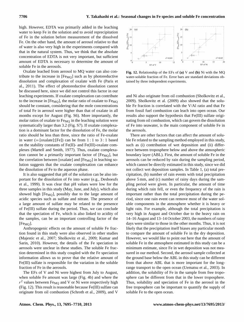
The EFs of V and Ni were highest from July to August,when soluble Fe amount was large (Fig. 4b) and where ther2 values between FeMQ and V or Ni were respectively high(Fig. 12). This result is reasonable because Fe(III) sulfate canoriginate from oil combustion (Schroth et al., 2009), and V

0

5

10

15

20

0 5 10 15

[Fe M

Q]/[

FeTo

tal]

(%)

r2=0.81

EF of V

0

5

10

15

20

0 5 10 15 20

r2=0.82

EF of Ni

[Fe M

Q]/[

FeTo

tal]

(%)

Figure 12

(b)(a)

Fig. 12. Relationship of the EFs of(a) V and (b) Ni with the MQwater-soluble fraction of Fe. Error bars are standard deviations ob-tained by three independent experiments.

and Ni also originate from oil combustion (Sholkovitz et al.,2009). Sholkovitz et al. (2009) also showed that the solu-ble Fe fraction is correlated with the V/Al ratio and that Fefrom fossil fuel combustion can leach into open ocean. Ourresults also support the hypothesis that Fe(III) sulfate origi-nating from oil combustion, which can govern the dissolutionof Fe into seawater, is the main component of soluble Fe inthe aerosols.

There are other factors that can affect the amount of solu-ble Fe related to the sampling method employed in this study,such as (i) contribution of wet deposition and (ii) differ-ence between troposphere below and above the atmosphericboundary layer (ABL). First, the amount of soluble Fe in theaerosols can be reduced by rain during the sampling period,which cannot be directly estimated in this study, since we didnot collect wet deposition samples. In Table 1, (a) total pre-cipitation, (b) number of rain events with total precipitationabove 5 mm, and (c) number of rainy days during the sam-pling period were given. In particular, the amount of timeduring which rain fell, or even the frequency of the rain isimportant rather than the total precipitation during the pe-riod, since one rain event can remove most of the water sol-uble components in the atmosphere whether it is heavy orlight rain. For example, although the total precipitation isvery high in August and October due to the heavy rain on14–16 August and 13–14 October 2003, the numbers of rainydays were similar to those in the other months. Thus, it is notlikely that the precipitation itself biases any particular monthto compare the amount of soluble Fe in the dry deposition.However, we would like to point out here that the amount ofsoluble Fe in the atmosphere estimated in this study can be aminimum estimate, since Fe in wet deposition was not mea-sured in our method. Second, the aerosol sample collected atthe ground base below the ABL in this study can be differentfrom that above ABL that is more important for the long-range transport to the open ocean (Uematsu et al., 2003). Inaddition, the solubility of Fe in the sample from free tropo-sphere can be different from that in the lower troposphere.Thus, solubility and speciation of Fe in the aerosol in thefree troposphere can be important to quantify the supply ofsoluble Fe to the open ocean.



Figure 13

(a) [FeTotal] for the year, by species (b) [FeSW] for the year, by species

Illite

HornblendeFe(III) sulfate

Ferrihydrite

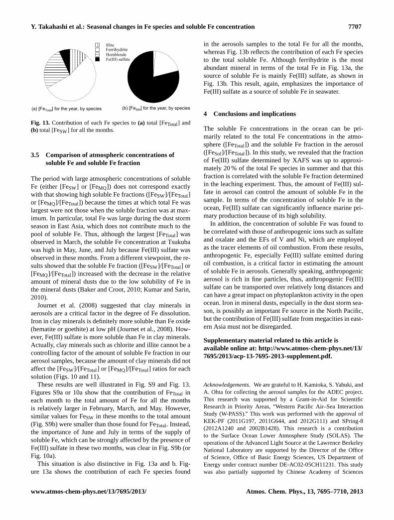
Fig. 13. Contribution of each Fe species to(a) total [FeTotal] and(b) total [FeSW] for all the months.

3.5 Comparison of atmospheric concentrations ofsoluble Fe and soluble Fe fraction

The period with large atmospheric concentrations of solubleFe (either [FeSW] or [FeMQ]) does not correspond exactlywith that showing high soluble Fe fractions ([FeSW]/[FeTotal]or [FeMQ]/[FeTotal]) because the times at which total Fe waslargest were not those when the soluble fraction was at max-imum. In particular, total Fe was large during the dust stormseason in East Asia, which does not contribute much to thepool of soluble Fe. Thus, although the largest [FeTotal] wasobserved in March, the soluble Fe concentration at Tsukubawas high in May, June, and July because Fe(III) sulfate wasobserved in these months. From a different viewpoint, the re-sults showed that the soluble Fe fraction ([FeSW]/[FeTotal] or[FeMQ]/[FeTotal]) increased with the decrease in the relativeamount of mineral dusts due to the low solubility of Fe inthe mineral dusts (Baker and Croot, 2010; Kumar and Sarin,2010).

Journet et al. (2008) suggested that clay minerals inaerosols are a critical factor in the degree of Fe dissolution.Iron in clay minerals is definitely more soluble than Fe oxide(hematite or goethite) at low pH (Journet et al., 2008). How-ever, Fe(III) sulfate is more soluble than Fe in clay minerals.Actually, clay minerals such as chlorite and illite cannot be acontrolling factor of the amount of soluble Fe fraction in ouraerosol samples, because the amount of clay minerals did notaffect the [FeSW]/[FeTotal] or [FeMQ]/[FeTotal] ratios for eachsolution (Figs. 10 and 11).

These results are well illustrated in Fig. S9 and Fig. 13.Figures S9a or 10a show that the contribution of FeTotal ineach month to the total amount of Fe for all the monthsis relatively larger in February, March, and May. However,similar values for FeSW in these months to the total amount(Fig. S9b) were smaller than those found for FeTotal. Instead,the importance of June and July in terms of the supply ofsoluble Fe, which can be strongly affected by the presence ofFe(III) sulfate in these two months, was clear in Fig. S9b (orFig. 10a).

This situation is also distinctive in Fig. 13a and b. Fig-ure 13a shows the contribution of each Fe species found

in the aerosols samples to the total Fe for all the months,whereas Fig. 13b reflects the contribution of each Fe speciesto the total soluble Fe. Although ferrihydrite is the mostabundant mineral in terms of the total Fe in Fig. 13a, thesource of soluble Fe is mainly Fe(III) sulfate, as shown inFig. 13b. This result, again, emphasizes the importance ofFe(III) sulfate as a source of soluble Fe in seawater.

4 Conclusions and implications

The soluble Fe concentrations in the ocean can be pri-marily related to the total Fe concentrations in the atmo-sphere ([FeTotal]) and the soluble Fe fraction in the aerosol([FeSol]/[FeTotal]). In this study, we revealed that the fractionof Fe(III) sulfate determined by XAFS was up to approxi-mately 20 % of the total Fe species in summer and that thisfraction is correlated with the soluble Fe fraction determinedin the leaching experiment. Thus, the amount of Fe(III) sul-fate in aerosol can control the amount of soluble Fe in thesample. In terms of the concentration of soluble Fe in theocean, Fe(III) sulfate can significantly influence marine pri-mary production because of its high solubility.

In addition, the concentration of soluble Fe was found tobe correlated with those of anthropogenic ions such as sulfateand oxalate and the EFs of V and Ni, which are employedas the tracer elements of oil combustion. From these results,anthropogenic Fe, especially Fe(III) sulfate emitted duringoil combustion, is a critical factor in estimating the amountof soluble Fe in aerosols. Generally speaking, anthropogenicaerosol is rich in fine particles, thus, anthropogenic Fe(III)sulfate can be transported over relatively long distances andcan have a great impact on phytoplankton activity in the openocean. Iron in mineral dusts, especially in the dust storm sea-son, is possibly an important Fe source in the North Pacific,but the contribution of Fe(III) sulfate from megacities in east-ern Asia must not be disregarded.

Supplementary material related to this article isavailable online at:http://www.atmos-chem-phys.net/13/7695/2013/acp-13-7695-2013-supplement.pdf.

Acknowledgements.We are grateful to H. Kamioka, S. Yabuki, andA. Ohta for collecting the aerosol samples for the ADEC project.This research was supported by a Grant-in-Aid for ScientificResearch in Priority Areas, “Western Pacific Air–Sea InteractionStudy (W-PASS).” This work was performed with the approval ofKEK-PF (2011G197, 2011G644, and 2012G111) and SPring-8(2012A1240 and 2002B1428). This research is a contributionto the Surface Ocean Lower Atmosphere Study (SOLAS). Theoperations of the Advanced Light Source at the Lawrence BerkeleyNational Laboratory are supported by the Director of the Officeof Science, Office of Basic Energy Sciences, US Department ofEnergy under contract number DE-AC02-05CH11231. This studywas also partially supported by Chinese Academy of Sciences


http://www.atmos-chem-phys.net/13/7695/2013/acp-13-7695-2013-supplement.pdf

http://www.atmos-chem-phys.net/13/7695/2013/acp-13-7695-2013-supplement.pdf


Visiting Professorship for Senior International Scientists (GrantNo. 2012T1Z0035) and National Natural Science Foundation ofChina (No. 41273112).

Edited by: A. B. Guenther

References

Aguilar-Islas, A. M., Wu, J., Rember, R., Johansen, A. M., andShank, L. M.: Dissolution of aerosol-derived iron in seawater:leach solution chemistry, aerosol type, and colloidal iron frac-tion, Mar. Chem., 120, 25–33, 2010.

Baker, A. R. and Croot, P. L.: Atmospheric and marine controls onaerosol iron solubility in seawater, Mar. Chem., 120, 4–13, 2010.

Baker, A. R. and Jickells, T. D.: Mineral particle size as a con-trol on aerosol iron solubility, Geophys. Res. Lett., 33, L17608,doi:10.1029/2006GL026557, 2006.

Beauchemin, S., Hesterberg, D., and Beauchemin, M.: Principalcomponent analysis approach for modeling sulfur K-XANESspectra of humic acids, Soil Sci. Soc. Am. J., 66, 83–91, 2002.

Bishop, J. K. B., Davis, R. E., and Sherman, J. T.: Robotic observa-tions of dust storm enhancement of carbon biomass in the NorthPacific, Science, 298, 817–821, 2002.

Boyd, P. W. and Ellwood, M. J.: The biogeochemical cycle of ironin the ocean, Nat. Geosci., 3, 675–682, 2010.

Boyd, P., Jickells, T. D., Law, C. S., Blain, S., Boyle, E. A., Bues-seler, K. O., Coale, K. H., Cullen, J. J., de Baar, H. J. W., Fol-lows, M., Harvey, M., Lancelot, C., Levasseu, M., Owens, N.,P. J., Pollard, R., Rivkin, R. B., Sarmiento, J., Schoemann, V.,Smetacek, V., Takeda, S., Tsuda, A., Turner, S., and Watson, A.J.: Mesoscale iron enrichment experiments 1993-2005: synthesisand future directions, Science, 315, 612–617, 2007.

Bruland, K. W. and Lohan, M. C.: Controls of Trace Metals in Sea-water, The Oceans and Marine Geochemistry, 6, Treatise on Geo-chemistry, Elsevier Ltd, 2003.

Buck, C. S., Landing, W. M., and Resing, J. A.: Par-ticle size and aerosol iron solubility: a high resolutionanalysis of Atlantic aerosols, Mar. Chem., 120, 14–24,doi:10.1016/j.marchem.2008.11.002, 2010.

Chen, Y. Z., Shah, N., Huggins, F. E., and Huffman, G.: Investiga-tion of the microcharacteristics of PM2.5 in residual oil fly ash byanalytical transmission electron microscopy, Environ. Sci. Tech-nol., 38, 6553–6560, 2004.

Claquin, T., Schulz, M., and Balkanski, Y.: Modeling the mineral-ogy of atmospheric dust sources, J. Geophys. Res., 104, 22243–22256, 1999.

David, R. L.: Handbook of Chemistry and Physics, 75th Edn., CRCPress, Inc., USA, 1994.

Desboeufs, K. V., Losno, R., Vimeux, F., and Cholbi, S.: The pHdependent dissolution of wind-transported Saharan dust, J. Geo-phys. Res., 104, 21287–21299, 1999.

Draxler, R. R. and Rolph, G. D.: HYSPLIT (HYbrid Single-ParticleLagrangian Integrated Trajectory) Model access via NOAAARL READY Website, available at:http://ready.arl.noaa.gov/HYSPLIT.php, NOAA Air Resources Laboratory, Silver Spring,MD, USA, 2003.

Duce, R. A., Unni, C. K. Ray, B. J., Prospero, J. M., and Merrill,J. T.: Long-range atmospheric transport of soil dust from Asia

to the tropical North Pacific: Temporal variability, Science, 209,1522–1524, 1980.

Duce, R. A., Liss, P. S., Merrill, J. T., Atlas, E. L., Buat-Menard, P.,Hicks, B. B., Miller, J. M., Prospero, J. M., Arimoto, R., Church,T. M., Ellis, W., Galloway, J. N., Hansen, L., Jickells, T. D.,Knap, A. H., Reinhardt, K. H., Schneider, B., Soudine, A., Tokos,J. J., Tsunogai, S., Wollast, R., and Zhou, M.: The atmosphericinput of trace species to the world ocean, Global Biogeochem.Cy., 5, 193–259, 1991.

Furukawa, T. and Takahashi, Y.: Oxalate metal complexes inaerosol particles: implications for the hygroscopicity of oxalate-containing particles, Atmos. Chem. Phys., 11, 4289–4301,doi:10.5194/acp-11-4289-2011, 2011.

Hasegawa, H., Maki, T., Asano, K., Ueda, K., and Ueda, K.: De-tection of iron(III)-binding ligands originating from marine phy-toplankton using cathodic stripping voltammetry, Anal. Sci., 20,89–93, 2004.

Ito, A.: Global modeling study of potentially bioavailable iron in-put from shipboard aerosol sources to the ocean, Globa. Bio-geochem. Cy., 27, 1–10, doi:10.1029/2012GB004378, 2013.

Jambor, J. L. and Dutrizac, J. E.: Occurrence and constitution of nat-ural and synthetic ferrihydrite, a widespread iron oxyhydroxide,Chem. Rev., 98, 2549–2585, 1998.

Jang, H. N., Seo, Y. C., Lee, J. H., Hwang, K. W., Yoo, J. I., Sok,C. H., and Kim, S. H.: Formation of fine particles enriched by Vand Ni from heavy oil combustion: Anthropogenic sources anddrop-tube furnace experiments, Atmos. Environ., 41, 1053–1063,2007.

Jickells, T. D. and Spokes, L. J.: Atmospheric Iron Inputs to theOceans, in: The Biogeochemistry of Iron in Seawater, edited by:Turner, D. R. and Hunter, K., SCOR/IUPAC Series, Wiley, 85–121, 2001.

Jickells, T. D., An, Z. S., Andersen, K. K., Baker, A. R., Berga-metti, G., Brooks, N., Cao, J. J., Boyd, P. W., Duce, R. A., Hunter,K. A., Kawahata, H., Kubilay, N., LaRoche, J., Liss, P. S., Ma-howald, N., Prospero, J. M., Ridgwell, A. J., Tegen, I., and Tor-res, R.: Global iron connections between desert dust, ocean bio-geochemistry, and climate, Science, 308, 67–71, 2005.

Journet, E., Desboeufs, K. V., Caquineau, S., and Colin, J. L.: Min-eralogy as a critical factor of dust iron solubility, Geophys. Res.Lett., 35, L07805, doi:10.1029/2007GL031589, 2008.

Kanai, Y., Ohta, A., Kamioka, H., Terashima, S., Imai, N., Mat-suhisa, Y., Kanai, M., Shimizu, H., Takahashi, Y., Kai, K., Xu,B., Hayashi, M., and Zhang, R.: Variation of concentrationsand physicochemical properties of aeolian dust obtained in eastChina and Japan from 2001 to 2002, Bull. Geol. Surv. Jpn., 54,251–267, 2003.

Kumar, A. and Sarin, M. M.: Aerosol iron solubility in a semiaridregion: temporal trend and impact of anthropogenic sources, Tel-lus, 62B, 125–132, 2010.

Kraemer, S. M.: Iron oxide dissolution and solubility in the presenceof siderophores, Aquat. Sci., 66, 3–18, 2004.

Kupiainen, K., Tervahattu, H., and Raisanen, M.: Experimentalstudies about the impact of traction sand on urban road dust com-position, Sci. Total Environ., 308, 175–184, 2003.

Kupiainen, K., Tervahattu, H., Raisanen, M., Makela, T., Aurela,M., and Hillamo, R.: Size and Composition of Airborne Particlesfrom Pavement Wear, Tires, and Traction Sanding, Environ. Sci.Technol., 39, 699–706, 2005.


http://dx.doi.org/10.1029/2006GL026557

http://dx.doi.org/10.1016/j.marchem.2008.11.002

http://ready.arl.noaa.gov/HYSPLIT.php

http://ready.arl.noaa.gov/HYSPLIT.php

http://dx.doi.org/10.5194/acp-11-4289-2011

http://dx.doi.org/10.1029/2012GB004378

http://dx.doi.org/10.1029/2007GL031589


Lam, P. J. and Bishop, J. K. B.: The continental margin is a keysource of iron to the HNLC North Pacific Ocean, Geophys. Res.Lett., 35, L07608, doi:10.1029/2008GL033294, 2008.

Langmann, B., Zaksek, K., Hort, M., and Duggen, S.: Volcanic ashas fertiliser for the surface ocean, Atmos. Chem. Phys., 10, 3891–3899, doi:10.5194/acp-10-3891-2010, 2010.

Leon, A., Kircher, O., Rothe, J., and Fichtner, M.: Chemical stateand local structure around titanium atoms in NaAlH4 doped withTiCl3 using X-ray absorption spectroscopy, J. Phys. Chem. B,108, 16372–16376, 2004.

Luo, C., Mahowald, N., Bond, T., Chuang, P. Y., Artaxo, P.,Siefert, R., Chen, Y., and Schauer, J.: Combustion iron distri-bution and deposition, Global Biogeochem. Cy., 22, GB1012,doi:10.1029/2007GB002964, 2008.

Mackie, D. S., Boyd, P. W., Hunter, K. A., and McTainsh, G.H.: Simulating the cloud processing of iron in Australian dust:pH and dust concentration, Geophys. Res. Lett., 32, L06809,doi:10.1029/2004GL022122, 2005.

Mahowald, N. M., Baker, A. R., Bergametti. G., Brooks, N.,Duce, R. A., Jickells, T. D., Kubilay, N., Prospero, J. M.,and Tegen, I.: Atmospheric global dust cycle and iron in-puts to the ocean, Global Biogeochem. Cy., 19, GB4025,doi:10.1029/2004GB002402, 2005.

Majestic, B. J., Schauer, J. J., and Shafer, M. M.: Application ofsynchrotron radiation for measurement of iron red-ox speciationin atmospherically processed aerosols, Atmos. Chem. Phys., 7,2475–2487, doi:10.5194/acp-7-2475-2007, 2007.

Manceau, A., Marcus, M. A., and Tamura, N.: Quantitative specia-tion of heavy metals in soils and sediments by synchrotron X-raytechniques, in: Applications of Synchrotron Radiation in Low-Temperature Geochemistry and Environmental Science, editedby: Fenter, P. and Sturchio, N. C., Reviews in Mineralogy andGeochemistry, Mineralogical Society of America, Washington,DC., 49, 341–428, 2002.

Manoli, E., Voutsa, D., and Samara, C.: Chemical characterizationand source identification/ apportionment of fine and coarse airparticles in Thessaloniki, Greece, Atmos. Environ., 36, 949–961,2002.

Marcus, M., MacDowell, A. A., Celestre, R., Manceau, A., Miller,T., Padmore, H. A., and Sublett, R. E.: Beamline 10.3.2 at ALS: ahard X-ray microprobe for environmental and materials sciences,J. Synchrotron Rad., 11, 239–247, 2004.

Marcus, M. A., Westphal, A. J., and Fakra, S. C.: Classificationof Fe-bearing species from K-edge XANES data using two-parameter correlation plots, J. Synchrotron Rad., 15, 463–468,2008.

Martell, A. E. and Smith, R. M.: Critical Stability Constants,Plenum Press, New York, 1982.

Martin, J. H.: Glacial-interglacial CO2 change: the iron hypothe-sism Paleoceanograpy, 5, 1–13, 1990.

Martin, J. H. and Fitzwater, S. E.: Iron deficiency limits phytoplank-ton growth in the north-east Pacific subarctic, Nature, 331, 341–343, 1988.

Martinez, E. and Maamaatuaiahutapu, K.: Island mass effect inthe Marquesas Islands: Time variation, Geophys. Res. Lett., 31,L18307, doi:10.1029/2004GL020682, 2004.

Oakes, M., Weber, R. J., Lai, B., Russell, A., and Ingall, E. D.:Characterization of iron speciation in urban and rural single par-ticles using XANES spectroscopy and micro X-ray fluorescence

measurements: investigating the relationship between speciationand fractional iron solubility, Atmos. Chem. Phys., 12, 745–756,doi:10.5194/acp-12-745-2012, 2012a.

Oakes, M., Ingall, E. D., Lai, B., Shafer, M. M., Hays, M. D., Liu,Z. G., Russell, A. G., and Weber, R. J.: Iron solubility relatedto particle sulfur content in source emission and ambient fineparticles, Environ. Sci. Technol., 46, 6637–6644, 2012b.

Ooki, A., Nishioka, J., Ono, T., and Noriki, S.: Size dependence ofiron solubility of Asian mineral dust particles, J. Geophys. Res.,114, D03202, doi:10.1029/2008JD010804, 2009.

Paris, R., Desboeufs, K. V., Formenti, P., Nava, S., and Chou, C.:Chemical characterisation of iron in dust and biomass burningaerosols during AMMA-SOP0/DABEX: implication for iron sol-ubility, Atmos. Chem. Phys., 10, 4273–4282, doi:10.5194/acp-10-4273-2010, 2010.

Paris, R., Desboeufs, K. V., and Journet E.: Variability of dust ironsolubility in atmospheric waters: Investigation of the role of ox-alate organic complexation, Atmos. Environ., 45, 6510–6517,2011.

Schroth, A. W., Crusius, J., Sholkovitz, E. R., and Bostick, B. C.:Iron solubility driven by speciation in dust sources to the ocean,Nat. Geosci., 2, 337–340, 2009.

Sedwick, P. N., Sholkovitz, E. R., and Church, T. M.: Impact of an-thropogenic combustion emissions on the fractional solubility ofaerosol iron: Evidence from the Sargasso Sea, Geochem. Geo-phys. Geosyst., 8, Q10Q06, doi:10.1029/2007GC001586, 2007.

Seinfeld, J. H. and Pandis, S. N.: Atmospheric Chemistry andPhysics: From Air Pollution to Climate Change, 2nd Edn., JohnWiley and Sons, NY, USA, 2006.

Seiter, J. M., Staats-Borad, K. E., Ginder-Vogel, M., and Sparks,D. L.: XANES spectroscopic analysis of phosphorus speciationin alum-amended poultry litter, J. Environ. Qual., 37, 477–485,2008.

Shi, Z., Krom, M. D., and Bonneville, S.: Formation of ironnanoparticles and increase in iron reactivity in mineral dustduring simulated cloud processing, Environ. Sci. Technol., 43,6592–6596, 2009.

Sholkovitz, E. R., Sedwick, P. N., and Church, T. M.: Influence ofanthropogenic combustion emissions on the deposition of solubleaerosol iron to the ocean: Empirical estimates for island sites inthe North Atlantic, Geochim. Cosmochim. Acta, 73, 3981–4003,2009.

Shukla, A. K., Raman, R. K., Choudhury, N. A., Priolkar, K. R., Sar-ode, P. R., Emura, S., Kumashiro, R.: Carbon-supported Pt–Fealloy as a methanol-resistant oxygen-reduction catalyst for directmethanol fuel cells, J. Electroanal. Chem., 563, 181–190, 2004.

Spokes, L. J. and Jickells, T. D.: Factors controlling the solubilityof aerosol trace metals in the atmosphere and on mixing into sea-water, Aqua. Geochem., 1, 355–374, 1996.

Takahashi, Y., Minai, Y., Ambe, S., Makide, Y., Ambe, F., andTominaga, T.: Simultaneous determination of stability constantsof humate complexes with various metal ions using multitracertechnique, Sci. Total Environ., 198, 61–71, 1997.

Takahashi, Y., Higashi, M., Furukawa, T., and Mitsunobu, S.:Change of iron species and iron solubility in Asian dust dur-ing the long-range transport from western China to Japan,Atmos. Chem. Phys., 11, 11237–11252, doi:10.5194/acp-11-11237-2011, 2011.


http://dx.doi.org/10.1029/2008GL033294


http://dx.doi.org/10.1029/2007GB002964

http://dx.doi.org/10.1029/2004GL022122

http://dx.doi.org/10.1029/2004GB002402


http://dx.doi.org/10.1029/2004GL020682


http://dx.doi.org/10.1029/2008JD010804



http://dx.doi.org/10.1029/2007GC001586




Taylor, S. R.: Abundance of chemical elements in the continentalcrust: a new table, Geochem. Cosmochim. Acta, 28, 1273–1285,1964.

Uematsu, M., Wang, Z. F., and Uno, I.: Atmospheric input of min-eral dust to the western North Pacific region based on direct mea-surements and a regional chemical transport model, Geophys.Res. Lett., 30, 1342, doi:10.1029/2002GL016645, 2003.

Uematsu, M., Hattori, H., Nakamura, T., Narita, Y., Jung, J., Mat-sumoto, K., Nakaguchi, Y., and Kumar, M. D.: Atmospherictransport and deposition of anthropogenic substances from theAsia to the East China Sea, Mar. Chem., 120, 108–115, 2010.

Var, F., Narita, Y., and Tanaka, S.: The concentration trend andseasonal variation of metals in the atmosphere in 16 Japanesecities shown by the results of National Air Surveillance Network(NASN) from 1974 to 1996, Atmos. Environ., 34, 2755–2770,2000.

Wilke, M., Farges, F., Petit, P., Brown Jr., G. E., and Martin, F.: Oxi-dation state and coordination of fe in minerals: An Fe K-XANESspectroscopic study, Am. Mineral., 86, 714–730, 2001.

Witter, A. E., Hutchins, D. A., Butler, A., and Luther, G. W.: Deter-mination of conditional stability constants and kinetic constantsfor strong model Fe-binding ligands in seawater, Mar. Chem., 69,1–17, 2000.

Xie, R. K., Seip, H. M., Leinum, J. R., Winje, T., and Xiao, J. S.:Chemical characterization of individual particles (PM10) fromambient air in Guiyang City, China, Sci. Total Environ., 343,262–272, 2005.


http://dx.doi.org/10.1029/2002GL016645

Documents

Seasonal changes in Fe species and soluble Fe ... · fate and oxalate originated from anthropogenic sources, ... joint project, ... pling with a reading precision of 10µg after stabilizing