Searching for the Tracy-Widom Distribution inNonequilibrium Processes(joint work with Herbert Spohn)

Christian B. Mendl

Stanford University, USA

October 19, 2016

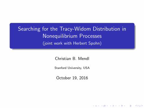
Outline and general concepts

Multiple scales:

microscopic FPU-type chains(molecular dynamics)

mesoscopic KPZ partial differentialequation

macroscopic fluid dynamics(hyperbolic conservation laws)

Uncover statistical Tracy-Widomdistribution in one-dimensional particlesystems

FPU-type anharmonic chains

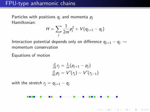
Particles with positions qj and momenta pjHamiltonian:

H =∑j

1

2mp2j + V (qj+1 − qj)

Interaction potential depends only on difference qj+1 − qj momentum conservation

Equations of motion

ddt rj = 1

m (pj+1 − pj)ddt pj = V ′(rj)− V ′(rj−1)

with the stretch rj = qj+1 − qj

FPU-type anharmonic chains

Particles with positions qj and momenta pjHamiltonian:

H =∑j

1

2mp2j + V (qj+1 − qj)

Interaction potential depends only on difference qj+1 − qj momentum conservation

Equations of motion

ddt rj = 1

m (pj+1 − pj)ddt pj = V ′(rj)− V ′(rj−1)

with the stretch rj = qj+1 − qj

FPU-type anharmonic chains: Conserved fields

Conserved fields:

~g(j) =

r jpje j

stretchmomentumenergy

with stretch r j = qj+1 − qj and energy e j = 12mp2j + V (rj)

Microscopic currents

~J (j) =

− 1mpj

−V ′(rj−1)− 1

mpjV′(rj−1)

microscopic conservation law

ddt~g(j , t) + ~J (j + 1, t)− ~J (j , t) = 0

FPU-type anharmonic chains: Conserved fields

Conserved fields:

~g(j) =

r jpje j

stretchmomentumenergy

with stretch r j = qj+1 − qj and energy e j = 12mp2j + V (rj)

Microscopic currents

~J (j) =

− 1mpj

−V ′(rj−1)− 1

mpjV′(rj−1)

microscopic conservation law

ddt~g(j , t) + ~J (j + 1, t)− ~J (j , t) = 0

Local thermodynamic equilibrium

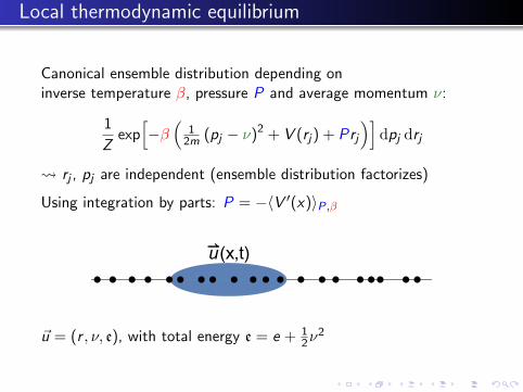
Canonical ensemble distribution depending oninverse temperature β, pressure P and average momentum ν:

1

Zexp[−β(

12m (pj − ν)2 + V (rj) + Prj

)]dpj drj

rj , pj are independent (ensemble distribution factorizes)

Using integration by parts: P = −〈V ′(x)〉P,β

u(x,t)

~u = (r , ν, e), with total energy e = e + 12ν

2

From microscopic to macroscopic conservation laws

microscopic ddt gα(j , t) + Jα(j + 1, t)− Jα(j , t) = 0

↓macroscopic ∂tuα(x , t) + ∂x jα(~u(x , t)) = 0

~u = (r , ν, e) and α = 1, 2, 3.

u(x,t)

Macroscopic Euler currents: (local) thermal averages of themicroscopic currents:

~j(r , ν, e) = 〈 ~J 〉P,ν,β =(−ν,P(r , e− 1

2ν2), νP(r , e− 1

2ν2))

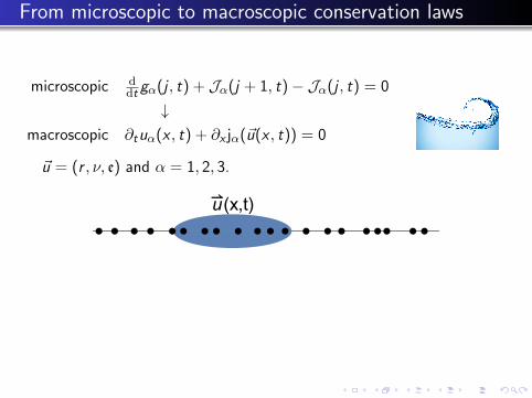
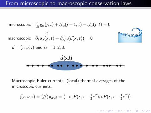
From microscopic to macroscopic conservation laws

microscopic ddt gα(j , t) + Jα(j + 1, t)− Jα(j , t) = 0

↓macroscopic ∂tuα(x , t) + ∂x jα(~u(x , t)) = 0

~u = (r , ν, e) and α = 1, 2, 3.

u(x,t)

Macroscopic Euler currents: (local) thermal averages of themicroscopic currents:

~j(r , ν, e) = 〈 ~J 〉P,ν,β =(−ν,P(r , e− 1

2ν2), νP(r , e− 1

2ν2))

From hydrodynamics to KPZ

Generic Euler equation (hyperbolic conservation law)

∂t u(x , t) + ∂x j(u(x , t)) = 0

Expand current to second order in u, add dissipation plus noise Langevin (stochastic Burgers) equation

∂tu(x , t) + ∂x(

j′(u)︸︷︷︸velocity c

u + 12 j′′(u)u2︸ ︷︷ ︸

nonlinear current

− D∂xu︸ ︷︷ ︸dissipation

+ ξ︸︷︷︸noise

)= 0,

where ξ(x , t) is space-time white noise.

Interpret as derivative of height function: u(x , t) = ∂xh(x , t) KPZ equation

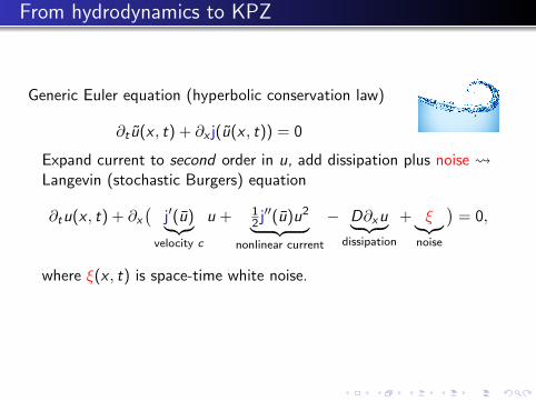
From hydrodynamics to KPZ

Generic Euler equation (hyperbolic conservation law)

∂t u(x , t) + ∂x j(u(x , t)) = 0

Expand current to second order in u, add dissipation plus noise Langevin (stochastic Burgers) equation

∂tu(x , t) + ∂x(

j′(u)︸︷︷︸velocity c

u + 12 j′′(u)u2︸ ︷︷ ︸

nonlinear current

− D∂xu︸ ︷︷ ︸dissipation

+ ξ︸︷︷︸noise

)= 0,

where ξ(x , t) is space-time white noise.

Interpret as derivative of height function: u(x , t) = ∂xh(x , t) KPZ equation

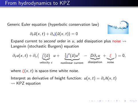
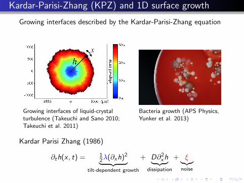
Kardar-Parisi-Zhang (KPZ) and 1D surface growth

Growing interfaces described by the Kardar-Parisi-Zhang equation

Growing interfaces of liquid-crystalturbulence (Takeuchi and Sano 2010;Takeuchi et al. 2011)

Bacteria growth (APS Physics,Yunker et al. 2013)

Kardar Parisi Zhang (1986)

∂th(x , t) = 12λ(∂xh)2︸ ︷︷ ︸

tilt-dependent growth

+ D∂2xh︸ ︷︷ ︸dissipation

+ ξ︸︷︷︸noise

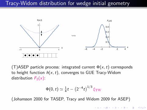
Tracy-Widom distribution for wedge initial geometry

-1 0 1x

1

h(x,t)

-6 -4 -2 2 4x

0.1

0.2

0.3

0.4

F2(x)

(T)ASEP particle process: integrated current Φ(x , t) correspondsto height function h(x , t), converges to GUE Tracy-Widomdistribution F2(x):

Φ(0, t) ' 14 t −

(2−4t

)1/3ξTW

(Johansson 2000 for TASEP, Tracy and Widom 2009 for ASEP)

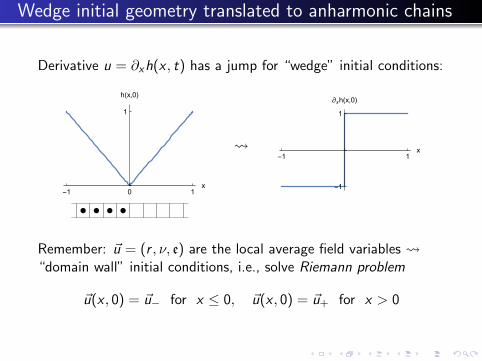
Wedge initial geometry translated to anharmonic chains

Derivative u = ∂xh(x , t) has a jump for “wedge” initial conditions:

-1 0 1x

1

h(x,0)

-1 1

x

-1

1

∂xh(x,0)

Remember: ~u = (r , ν, e) are the local average field variables “domain wall” initial conditions, i.e., solve Riemann problem

~u(x , 0) = ~u− for x ≤ 0, ~u(x , 0) = ~u+ for x > 0

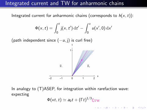
Integrated current and TW for anharmonic chains

Integrated current for anharmonic chains (corresponds to h(x , t)):

Φ(x , t) =

∫ t

0j(x , t ′) dt ′ −

∫ x

0u(x ′, 0)dx ′

(path independent since (−u, j) is curl free)

u- u

+

-2 -1 0 1 2x

1

t

In analogy to (T)ASEP, for integration within rarefaction wave:expecting

Φ(vt, t) ' a0t + (Γt)1/3ξTW

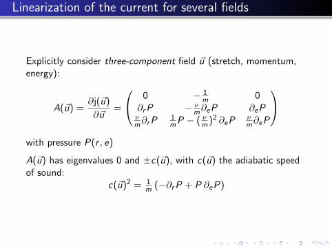
Linearization of the current for several fields

Explicitly consider three-component field ~u (stretch, momentum,energy):

A(~u) =∂j(~u)

∂~u=

0 − 1m 0

∂rP − νm∂eP ∂eP

νm∂rP

1mP − ( νm )2 ∂eP

νm∂eP

with pressure P(r , e)

A(~u) has eigenvalues 0 and ±c(~u), with c(~u) the adiabatic speedof sound:

c(~u)2 = 1m (−∂rP + P ∂eP)

Generalization to several fields

Three-component noisy Burgers equation:

∂t~u + ∂x(A~u + 1

2〈~u, ~H~u〉 − ∂x D~u + B~ξ(x , t))

= 0

Hessians: Hαγγ′ = ∂uγ∂uγ′ jα, jα = 〈Jα〉

Initial correlations: 〈uα(x , 0); uα′(x ′, 0)〉 = Cαα′ δ(x − x ′)

Diagonalization (transformation to normal modes):

~φ = R~u, RAR−1 = diag(−c , 0, c), RCRT = 1

∂tφα + ∂x(cαφα + 1

2〈~φ,Gα~φ〉 − ∂xDφα + B~ξ(x , t)

)= 0

α = 1α = -1

α = 0

-1000 -500 500 1000x

0.002

0.004

0.006

0.008

Sαα# (x,t)

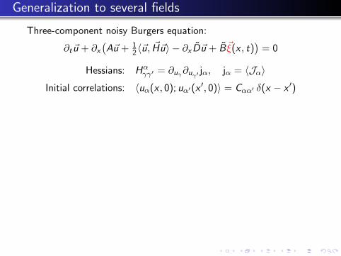
Generalization to several fields

Three-component noisy Burgers equation:

∂t~u + ∂x(A~u + 1

2〈~u, ~H~u〉 − ∂x D~u + B~ξ(x , t))

= 0

Hessians: Hαγγ′ = ∂uγ∂uγ′ jα, jα = 〈Jα〉

Initial correlations: 〈uα(x , 0); uα′(x ′, 0)〉 = Cαα′ δ(x − x ′)

Diagonalization (transformation to normal modes):

~φ = R~u, RAR−1 = diag(−c , 0, c), RCRT = 1

∂tφα + ∂x(cαφα + 1

2〈~φ,Gα~φ〉 − ∂xDφα + B~ξ(x , t)

)= 0

α = 1α = -1

α = 0

-1000 -500 500 1000x

0.002

0.004

0.006

0.008

Sαα# (x,t)

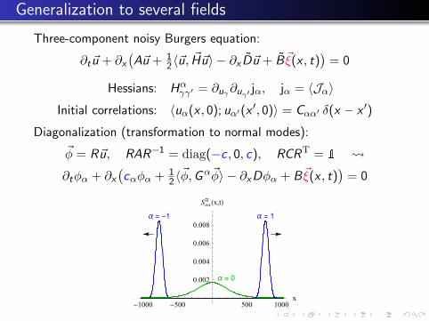
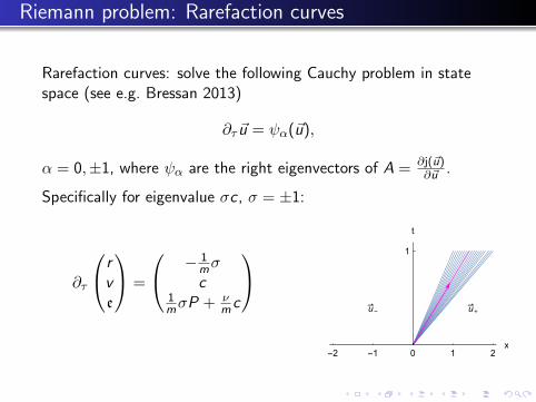
Riemann problem: Rarefaction curves

Rarefaction curves: solve the following Cauchy problem in statespace (see e.g. Bressan 2013)

∂τ ~u = ψα(~u),

α = 0,±1, where ψα are the right eigenvectors of A = ∂j(~u)∂~u .

Specifically for eigenvalue σc , σ = ±1:

∂τ

rve

=

− 1mσc

1mσP + ν

mc

u- u

+

-2 -1 0 1 2x

1

t

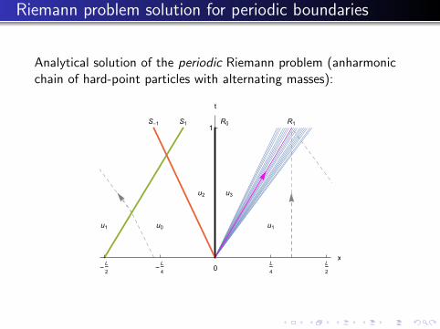
Riemann problem solution for periodic boundaries

Analytical solution of the periodic Riemann problem (anharmonicchain of hard-point particles with alternating masses):

R1S1 R0S-1

u0 u1

u2 u3

u1

-L

2-L

40

L

4

L

2

x

1

t

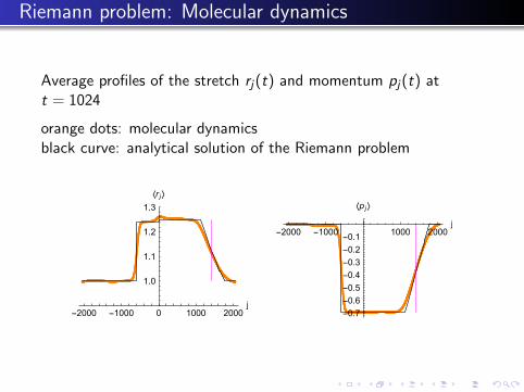
Riemann problem: Molecular dynamics

Average profiles of the stretch rj(t) and momentum pj(t) att = 1024

orange dots: molecular dynamicsblack curve: analytical solution of the Riemann problem

-2000 -1000 0 1000 2000j

1.0

1.1

1.2

1.3

⟨r j ⟩

-2000 -1000 1000 2000j

-0.7

-0.6

-0.5

-0.4

-0.3

-0.2

-0.1

⟨pj ⟩

Transformation to normal modes

Projected current components (with asymptotic value subtracted):

Φ]σ(t) =

⟨ψσ|~Φ(vt, t)− t(~j(~uv)− v~uv)

⟩with ψσ the left eigenvectors of A(~uv)

Φ]1(t) results from perturbations propagating with velocity v along

the magenta observation ray expecting

Φ]1(t) ' (Γ1t)1/3ξTW

Components σ = −1, 0 pick up samples from essentiallyindependent space-time regions central limit type behavior

Φ]σ(t) ' (Γσt)1/2ξG, σ = 0,−1,

with ξG a normalized Gaussian random variable

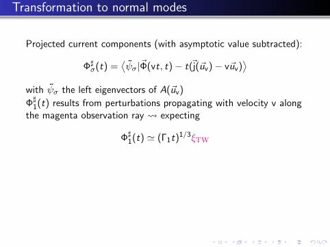
Transformation to normal modes

Projected current components (with asymptotic value subtracted):

Φ]σ(t) =

⟨ψσ|~Φ(vt, t)− t(~j(~uv)− v~uv)

⟩with ψσ the left eigenvectors of A(~uv)

Φ]1(t) results from perturbations propagating with velocity v along

the magenta observation ray expecting

Φ]1(t) ' (Γ1t)1/3ξTW

Components σ = −1, 0 pick up samples from essentiallyindependent space-time regions central limit type behavior

Φ]σ(t) ' (Γσt)1/2ξG, σ = 0,−1,

with ξG a normalized Gaussian random variable

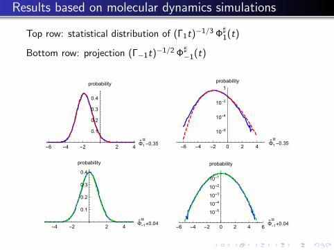
Results based on molecular dynamics simulations

Top row: statistical distribution of (Γ1t)−1/3 Φ]1(t)

Bottom row: projection (Γ−1t)−1/2 Φ]−1(t)

-6 -4 -2 2 4Φ1

#-0.35

0.1

0.2

0.3

0.4

probability

-6 -4 -2 0 2 4Φ1

#-0.35

10-6

10-4

10-2

1probability

-4 -2 2 4Φ-1

#+0.04

0.1

0.2

0.3

0.4

probability

-6 -4 -2 0 2 4 6Φ-1

#+0.04

10-510-410-310-210-1

probability

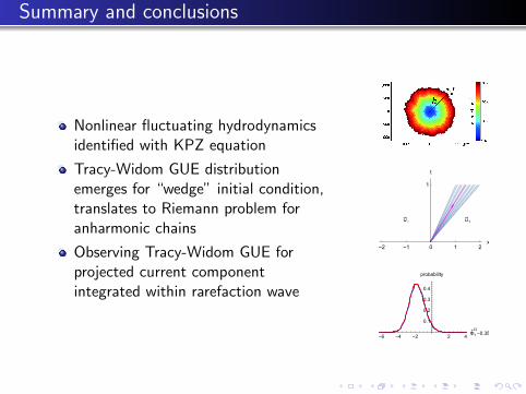
Summary and conclusions

Nonlinear fluctuating hydrodynamicsidentified with KPZ equation

Tracy-Widom GUE distributionemerges for “wedge” initial condition,translates to Riemann problem foranharmonic chains

Observing Tracy-Widom GUE forprojected current componentintegrated within rarefaction wave

u- u

+

-2 -1 0 1 2x

1

t

-6 -4 -2 2 4Φ1

#-0.35

0.1

0.2

0.3

0.4

probability

References I

Bressan, A. (2013). “Modelling and Optimisation of Flows on Networks,Cetraro, Italy 2009”. In: vol. Lecture Notes in Mathematics 2062.Springer. Chap. Hyperbolic conservation laws: An illustrated tutorial,pp. 157–245.

Johansson, K. (2000). “Shape fluctuations and random matrices”. In:Commun. Math. Phys. 209, pp. 437–476.

Mendl, C. B. and Spohn, H. (2013). “Dynamic correlators of FPU chainsand nonlinear fluctuating hydrodynamics”. In: Phys. Rev. Lett. 111,p. 230601.

– (2014). “Equilibrium time-correlation functions for one-dimensionalhard-point systems”. In: Phys. Rev. E 90, p. 012147.

– (2015). “Current fluctuations for anharmonic chains in thermalequilibrium”. In: J. Stat. Mech. 2015, P03007.

– (2016a). “Searching for the Tracy-Widom distribution innonequilibrium processes”. In: Phys. Rev. E 93, 060101(R).

– (2016b). “Shocks, rarefaction waves, and current fluctuations foranharmonic chains”. In: J. Stat. Phys.

References II

Spohn, H. (2014). “Nonlinear fluctuating hydrodynamics for anharmonicchains”. In: J. Stat. Phys. 154, pp. 1191–1227.

Takeuchi, K. A. and Sano, M. (2010). “Universal Fluctuations ofGrowing Interfaces: Evidence in Turbulent Liquid Crystals”. In: Phys.Rev. Lett. 104, p. 230601.

Takeuchi, K. A. et al. (2011). “Growing interfaces uncover universalfluctuations behind scale invariance”. In: Sci. Rep. 1, p. 34.

Tracy, C. A. and Widom, H. (2009). “Asymptotics in ASEP with stepinitial condition”. In: Commun. Math. Phys. 290, pp. 129–154.

Yunker, P. J. et al. (2013). “Effects of particle shape on growth dynamicsat edges of evaporating drops of colloidal suspensions”. In: Phys. Rev.Lett. 110 (3), p. 035501.