Searching for the Appropriate Measure of Multilateral

© 2014 Nicolaus Copernicus University. All rights reserved. http://www.dem.umk.pl/dem

D Y N A M I C E C O N O M E T R I C M O D E L S DOI: http://dx.doi.org/10.12775/DEM.2014.002 Vol. 14 (2014) 29−49

Submitted June 25, 2014 ISSN Accepted December 23, 2014 1234-3862

Natalia Drzewoszewska*

Searching for the Appropriate Measure of Multilateral Trade-Resistance Terms in the Gravity Model

of Bilateral Trade Flows

A b s t r a c t. The aim of the paper is to compare different approximations of multilateral trade-resistance in the gravity model and the influence of their use on estimation results for models of EU-trade. Three synthetic variables: for bilateral trade costs, exporter’s and import-er’s remoteness are used as an alternative for including time-varying country effects. Results indicate significant impact of those variables but not wholly compatible with the theory. Estimated coefficients of trade determinants, including Euro’s effects, have expected values in both approaches only if the FE estimator is applied.

K e y w o r d s: international trade, panel data, gravity model, multilateral trade-resistance terms, bilateral trade costs, globalization in the XXI century, Euro‘s effect

J E L Classification: F10, F14, F15, C23, C24, C26.

Introduction

The gravity model is a common tool for analyzing the flows of interna-tional trade. The characteristics of panel data allow for taking into considera-tion unit specific effects with regard to territorial units covered by the study, as well as time effects referring to the years under analysis. Therefore,

* Correspondence to: Natalia Drzewoszewska, Nicolaus Copernicus University, Depart-

ment of Statistics and Econometrics, ul. Gagarina 13a, 87-100 Toruń, e-mail: [email protected].

This paper was written during the author's research stay at the Chair of Statistics and Econometrics at Justus Liebig University Giessen. The author would like to thank Prof. Dr. Peter Winker for the work conditions, his encouragement and helpful suggestions.

Natalia Drzewoszewska

DYNAMIC ECONOMETRIC MODELS 14 (2014) 29–49

30

it assists in controlling for unobserved heterogeneity, which could not be accounted for by explanatory variables in the model, which is useful for such a macroeconomic study. An additional incentive for using the gravity model is that the necessary data is relatively easily available. Estimation results of a majority of studies described hereinafter are quite similar for the main variables in the model – differences come from the different test samples and different time periods, as well as from different estimation methods used in the research. Focusing on theoretical assumptions of the model can easily explain the inaccuracy of some empirical trade analyses based on the gravity model. According to the theory of Anderson and van Wincoop (2003), decisions about international trade essentially depend on the relative trade costs, which are however not easy to measure. One of the aims of this study is to identify the best measure of these costs, which will cover the multilateral trade-resistance, both for exporter and importer. Estimated panel gravity models include typical explanatory variables: national income, measure of bilateral distance and the set of dummy variables for common border, common lan-guage and access to the sea. Additionally, considering the utility of the gravity model by the test of trade-agreement effect, in former analysis there were the dummy variables used to describe the participation in The Econom-ic and Monetary Union (Micco et al., 2002, 2003; Maliszewska, 2004). Another purpose is the analysis of the international trade between EU countries, which create an integrated, relatively homogenous area, where such variables like tariffs or rates of exchange that do not have to be includ-ed in the model. Globalization is often defined as the growing integration of economies and societies around the world1 “mainly by free trade and free capital mobility, but also by easy or uncontrolled migration” (Daly, 1999), “leading to the notion of a borderless global or planetary economy” (Avi-nash, 2000), which makes the European Union a great example of the glob-alized economies. Globalization in the XXI century is a specific time – there are deeper and broader changes in the global economy – spread of the “New Economy” as well as the new information and communication technology (ICT), what is pointed out in recent studies (Ramos and Ballell, 2009; Farhadi et al., 2012; García-Muñiz and Vicente, 2014). Friedman describes 1999 as the year of the Internet, when the globalization started a new era, opened for outsourc-ing, offshoring and other new activities changing the global trade structure

1 Definition used by The World Bank Group, 2001.

Searching for the Appropriate Measure of Multilateral Trade-Resistance Terms…


31

(Friedman, 1999). That is the reason choosing 1999 the starting year of the analyzing time period. Three research hypotheses were put forward within the framework of the carried out objective. The first assumes that the travel time between cen-troids of countries is a good base for approximation of bilateral trade costs. Following the second hypothesis, bilateral trade flows increase if exchange partners are members of the Eurozone. The third hypothesis assumes that synthetic variables of bilateral costs and remoteness are accurate approxima-tion of multilateral trade-resistance terms for EU countries. Two first parts of the paper discuss the theoretical assumptions of the gravity model for trade flows and the problems with its estimation. The third focuses on the description of the new measures for multilateral trade-resistance terms. The final part presents the results of conducted research.

1. Theory of the Gravity Model of Bilateral Trade Flows

The first gravity equation was based only on empirical research of Tin-bergen (1962). Inspired by Newton's law of universal gravitation, author presented following “traditional” gravity equation for trade2:

,3210

oddood DXXY (1)

where: odY – volume of trade flow from country o (origin) to country d (des-

tination), do X,X – national income of countries o and d (GNP volumes),

odD – physical distance between the two countries. More generally, we can describe the gravity model by four forces: G – external (global) factors expressing “gravitational constant”, although it is only held constant in the cross-section, oS , dM – specific factors of origin

and destination factors expressing their “masses”, and od – negative factors expressing the trade costs, with the following form:

,0 oddod MSGY (2)

The gravity model with panel data structure can be written in following logarithmic form:

,,,3,2,10, todtodtdtotod εDXXY (3)

2 This equation implies that exports have a constant elasticity with respect to each of three

explanatory variables – what means that a 1 per cent increase in the GNP of country d always results in an increase of

2 per cent in the exports of the supplying country o.



32

where: Nod ,...,2,1, , tod ,Y – flow values (log) between regions o,d –

object’s number3, t=1,2,...,T – number of time period, t,oX , t,dX – explana-

tory variables values (log) respectively for origin and destination regions,

t,odD – bilateral trade costs, including distance between regions (log),

3210 ,,, – structural parameters of the model4, tod ,ε – random compo-

nent. Tinbergen (1962) also extended his model for 18 developed countries by dummy variables of common border, Commonwealth preference and Bene-lux preference and, in the second case, by the Gini coefficient of export commodity concentration. Further research of econometricians was expand-ed by additional variables and effects, like time effects or country pair ef-fects. Nevertheless, the gravity equation still needed the theoretical assump-tions, which became a key issue in the following years. The theory of gravity model was proposed by Anderson (1979), Bergstrand (1989), Deardoff (1998), Eaton-Kortum (2002) and Anderson and van Wincoop (2003). The last one was named as “the final structural gravity equation” and it passes now for the most accurate description of reality. The most important part relates to the relative trade costs, which are included in the model as multi-lateral trade-resistance (MTR) terms. Namely, these two terms measure the exporter's and importer's joint average trade resistance (in terms of trade barriers), which each of them faces to all their other potential trading part-ners. For instance, if there is a rise in trade barriers between importing coun-try d and all its other possible trading partners (inward MTR rises), the rela-tive price of the exporting country o’s products will decrease and trade flows between o and d will increase. Likewise, if outward MTR rises, overall de-mand on o’s exported products will slow down, thus reducing the price oP , which, under conditions of the constant trade barriers, will consequently increase trade flows between both countries. The new structural gravity equation takes the form of:

,1

do

odW

dood P

t

X

XXEXPORT (4)

3 In case of panel gravity models, which analyze trade flows, a pair of regions represents

an object (unit), namely d,oi . For N analyzed regions NN 2 objects are included in

the study, i.e. pairs of trading partners. 4 Prediction that 11 , 12 leads to the unit-income-elasticity model, what was often

assumed by researchers in the studies.



33

with: outward (exporter’s) multilateral trade-resistance:

,1

1Wd

o d

odo

X

X

P

t

(5)

and inward (importer’s) multilateral trade-resistance:

.1

1Wo

o o

odd

X

XtP

(6)

where: oX , dX – national income values of both trading countries, WX –

World’s income, odt – trade cost factor reflecting bilateral trade resistance between country o and d, – elasticity of substitution. The conception of multilateral trade-resistance of trading countries is intuitively convincing since all the countries have a lot of potential alterna-tive trading partners and relationships with them that influence the bilateral trade-resistance. Hence the trade impediments between countries should not be approximated only by the bilateral trade costs. Moreover, the import and export of more developed and wealthy countries should be easier, which is also expressed in the above form of gravity equation by implementing the income shares in the total World income. Omitting the theoretically motivat-ed MTR terms in the gravity models leads to the systematic bias in coeffi-cient estimates of bilateral trade-cost variables. This form of gravity model, acclaimed to be the most accurate one because of using relative differences between countries, was easily expanded to describe another foreign flows, namely migration flows (Anderson, 2011).

2. Difficulties with Empirical Research Based on the Gravity Model of Trade Flows Using Panel Data

The multiplicative nature of the gravity equation, quality of available database, characteristics of panel data or the big amount of missing data yield many potential problems with a solid empirical analysis. Among the biggest problems occurring by estimating the panel data gravity models are5: multitude of zero-observations (log-linearization is not feasible in these

cases),

5 More problems with trade data are presented in Feenstra et al. (2001). For essential ref-

erence on panel-data models see Hsiao (2003).



34

error terms in the usual log-linear form of the gravity equation are heter-oscedastic (which violates the assumption that error term should be sta-tistically independent from the regressors, using OLS-method after the log-linearization leads to inconsistent estimates of the elasticity of inter-est, the NLS estimator is in turn very inefficient, as it ignores the hetero-scedasticity),

variance of the error term is not constant (NLS estimator is not optimal) trade data are suffering from rounding errors (that leads to the bias of

estimates), MTR terms should be included in the gravity model of bilateral flows,

but they are not directly observable. There are many potential methods that can more or less overcome the foregoing problems. One way with the first problem is dropping the pairs with zero from the trade-data set, what allows for using OLS estimation method. Another way is to keep these observations by adding a constant to zero-observations, for instance ( 1ijY ) and use again OLS method, what can

be found in Martinez-Zarzoso (2007), Westerlund and Wilhelmsson (2009), or use tobit model for panel data (Soloaga and Winters, 2001; Baldwin and DiNino, 2006; Tripathi and Leitão, 2013). However, all three of these meth-ods lead to inconsistent estimates (especially by tobit models, where estima-tion results depend on the chosen constant). To avoid this problem, Santos Silva and Tenreyro (2006) proposed the use of PPML (Poisson pseudo max-imum likelihood) estimator6 in levels, which not only deals with zero-value observations, but also can be easily adapted in models with endogenous re-gressors, providing unbiased estimates in the presence of heteroske-dasticity, where all observations are weighted equally. The choice of an accurate estimation method in face of all the problems connected with the gravity model is never infallible; hence the common way is to use several estimation methods, appropriate to considering case of study. Every estimator has pros and cons7 and the inference based on the only one method is not advisable. Even using the Hausman test by pointing out the right version of model between RE and FE is not practiced since the form of both models is not the same (the lack of constant variables in FE-model) and the assumption about individual fixed effects between trading

6 Previously authors used the gamma PML (GPML), which gave good results, but is very

sensitive to measurement errors – as it gives an extra weight to the noiser observations. The PPML method was originally proposed by McCullagh and Nelder (1989).

7 Details about majority of estimation methods of gravity model are presented by Gómez-Herrera (2013).



35

pairs in this case seems to always be the right one. However, the readiness of researchers to know the coefficients by constant variables leads to imple-menting more estimation methods. The comparison of the coefficients gives an answer to the questions asked in the hypotheses of the research. Interest-ing research of Gómez-Herrera (2013) includes a comparison of many esti-mation methods (truncated OLS, OLS ( 1ijY ), tobit, probit – with Heck-

man’s approach8, RE, FE and PPML), where gravity model, despite of physical distance and dummies (common border, common language, same country and participation in trade agreements)9 among regressors, included also exporter and importer time varying effects. The results of comparison of several techniques with a dataset covering 80% of World trade induce to choose the Heckman sample selection model as the preferred estimation method within nonlinear techniques when data are heteroskedastic, but this approach is preferred when the data also contain a significant proportion of zero observations – what is natural by analyzing 80% of the World trade. The need of using MTR terms is the result of new structural gravity equation proposed by Anderson and van Wincoop (2003), which logarithmic form is following:

,,,4

,4,3,2,10,

todtd

totodtdtotod

επ

P

tXXEXPORT

(7)

where: 31 . There are two ways to take MTR on board in the gravity model: 1) creat-ing synthetic variables for both countries – remoteness10 – or: 2) including time-varying individual effects for both countries in the gravity model (the dummy variables identifying the exporter and importer) 11.

8 See Bikker and de Vos (1992), Linders and de Groot (2006), Martin and Pham (2008).

9 The formula to compute the effect of dummy-variables is following: %ibe 1001 ,

where ib is the estimated coefficient. 10 Wei (1996) defined as the log of GDP-weighted average distance to all other countries. 10 The use of simulation method allows to obtain MTR as well. However, because of the

complex calculation problem, this method is rarely taken into consideration by researchers. Anderson and van Wincoop (2003) used non-linear programming to include MTR terms, assuming that elasticity of substitution equal to 8 . However, Feenstra (2002) showed that it is possible to apply importer and exporter fixed effects to obtain approximately similar results. Alternatively, Baier and Bergstrand (2009) introduced variables of MR approxima-tions which produce consistent estimates, using Taylor approximation. This approach were used also by Behar and Nelson (2012).



36

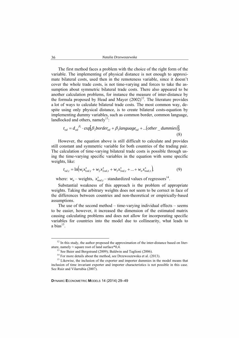
The first method faces a problem with the choice of the right form of the variable. The implementing of physical distance is not enough to approxi-mate bilateral costs, used then in the remoteness variable, since it doesn’t cover the whole trade costs, is not time-varying and forces to take the as-sumption about symmetric bilateral trade costs. There also appeared to be another calculation problems, for instance the measure of inter-distance by the formula proposed by Head and Mayer (2002)12. The literature provides a lot of ways to calculate bilateral trade costs. The most common way, de-spite using only physical distance, is to create bilateral costs-equation by implementing dummy variables, such as common border, common language, landlocked and others, namely13:

._...exp 321 dummiesotherlanguageborderdt odododod

(8)

However, the equation above is still difficult to calculate and provides still constant and symmetric variable for both countries of the trading pair. The calculation of time-varying bilateral trade costs is possible through us-ing the time-varying specific variables in the equation with some specific weights, like:

,...ln ,,33,22,11,s

tnodns

tods

tods

todtod xwxwxwxwt (9)

where: nw – weights, st,nodx – standardized values of regressors14.

Substantial weakness of this approach is the problem of appropriate weights. Taking the arbitrary weights does not seem to be correct in face of the differences between countries and non-theoretical or empirically-based assumptions. The use of the second method – time-varying individual effects – seems to be easier, however, it increased the dimension of the estimated matrix causing calculating problems and does not allow for incorporating specific variables for countries into the model due to collinearity, what leads to a bias15.

12 In this study, the author proposed the approximation of the inter-distance based on liter-

ature, namely ≈ square root of land surface*0,4. 13 See Baier and Bergstrand (2009); Baldwin and Taglioni (2006). 14 For more details about the method, see Drzewoszewska et al. (2013). 15 Likewise, the inclusion of the exporter and importer dummies in the model means that

inclusion of time invariant exporter and importer characteristics is not possible in this case. See Ruiz and Vilarrubia (2007).



37

Facing the problems above, there is no standard way to incorporate MTR in the gravity model so far. In the literature, there is a lot of research with exporter and importer effects in gravity model of bilateral trade flows, e.g. Rose and Wincoop (2001), Baltagi (2003), Ruiz and Vilarrubia (2007). The popular practise is to include country-pair effects as well, eg. Glick and Rose (2002), Baltagi (2003), Micco et al. (2003), Fratianni and Hoon-Oh (2007), Fidrmuc (2008), Bussière and Schnatz (2009). Furthermore, using time ef-fects in the gravity model is a common issue now, as it replaces global cir-cumstances, shocks, ect. Another way could be spatial modeling – in the research of FDI Fernández-Avilésa et al. (2012) proposed a simple FDI-based measure of financial distance with the use of spatial techniques. The remoteness variables for exporting and importing countries used in foregoing studies have different formulas, are both time-varying (Baldwin and Taglioni, 2006) and fixed (Fidrmuc, 2001; Ruiz and Vilarrubia, 2007). For instance, Head (2003) calculates remoteness as a country’s average weighted distance from its trading partners, where weights are the partner countries’ shares of world GDP. The physical distance between trading countries approximates bilateral trade costs since the first application of gravity model. The coefficient of this variable in estimated models is always negative in all the empirical analysis, what makes it a common measure used by researchers. However, the trade costs are created primarily by transport costs, which are depended on the quality of transport infrastructure, tariffs, prices, as well as on the distance. An alternative measure of bilateral trade costs for UE countries is prosed in the empirical part of this study.

3. A New Measure of Remoteness

The new formula of remoteness variables, proposed in this study, allows for using time-varying bilateral costs, which according to the strong assump-tion in Anderson and van Wincoop (2003) theory are symmetric. Besides, using the distance between countries to describe their bilateral costs leads to the constant remoteness, which is another unreal assumption. The formulas of three synthetic variables – bilateral costs t,odt , exporter’s remoteness

t,odREM and importer’s remoteness t,doREM – are following:

,_' ,

,tod

odtod OPENNESSSIMPORTER

DISTANCEt (10)

where:



38

._

_',

,,,

td

tdotodtod IMPORTTOTAL

EXPORTEXPORTOPENNESSSIMPORTER

(11)

Bilateral trade costs (10) became time-varying in this approach, which suits better to reality – trading costs are not constant over time and the psy-chical distance, especially in the era of globalization XXI century, does not lower the trade flows as much as 50 years ago. Here the distance between countries, measured by travel time between the centroids of trading coun-tries, is divided by share of bilateral trade exchange in the total import of importing country. Moreover, this method reflects the theoretical signifi-cance of importer’s demand in the final amount of bilateral trade flows.

Importer’s demand is also underlined by the following form of export-er’s remoteness variable:

,_, ,

,,

dok ttk

toktod INCOMEWORLDINCOME

tREMOTENESS (12)

which is the sum of bilateral costs divided by importer’s income share in the World’s total income. It is expected that a relatively richer importing country will have a larger overall demand, hence the export to this country will be relatively easy (exporter’s remoteness is smaller then). In this approach, importer’s remoteness variable includes analogously the exporter’s income share in the World’s total income as a weight in the weighted average:

._, ,

,,

dok ttk

tkdtdo INCOMEWORLDINCOME

tREMOTENESS (13)

However, the denominator of importer’s remoteness variable above un-derlines exporter’s condition, what (being still potential good weight) does not play substantial role in the demand of importing country16. Potentially better weight would be a share of bilateral export from the importer in his total export, since it better expresses importer’s condition and also reflects the interrelation with his trading partner. Hence, an alternative measure for importer’s remoteness is the following:

16 In macroeconomic theory, import is defined as a function of the domestic absorption A

(total demand for all final marketed goods and services) and the real exchange rate , taking the form of: ),A(fI . See Burda and Wyplosz (2005).



39

._, ,,

,,

dok tdtdk

tkdtdo EXPORTTOTALEXPORT

tREMOTENESS (14)

Comparison of the estimated coefficient’s sign of both above importer’s remoteness synthetic variables would give an answer if the second form, more economically justifiable, contains a better approximation of inward multilateral resistance. According to the theoretical assumptions of Anderson and van Wincoop (2003), the MTR terms should have a positive impact on bilateral trade flows. According to the theory, estimation results of models with remoteness synthetic terms and models with countries time-varying specific effects should have similar estimates of the rest of the variables. This could confirm that the created synthetic variables are a good approximation of MTR, which allows for estimation of their exact influence, also giving an opportunity to use more estimators, like PPML or HT. The model to compare has the fol-lowing form:

,,,5

,43,2,10,

todtod

todttdtotod

εX

tIIIEXPORT

(15)

where: t,dt,o ,II – time-varying individual effects, tI – time effects, t,odt –

bilateral trade costs, t,odX – set of dummies for the trading pair.

An easier way to estimate MTR can be the assumption that MTR is con-stant over time, what allows for using only fixed individual effects for both countries, with lower dimension of the estimating matrix. However, this assumption is advisable in the case of relatively short time period, so it is not considered in this study.

4. Gravity Model of Bilateral Trade Flows for EU Countries in the Period of 1999–2011 – Empirical Results

The data used in this study consists of a sample of 25 EU countries, with the following database-sources: Comtrade/OECD, WDI and Google Maps application. In order to analyze the trade in the era of globalization XXI century, the chosen time period of research is opened by “the year of the Internet” and includes the last year of available data. Variables included in the analysis are presented in Table 1. The first step of research was to look for an alternative variable that could replace the physical distance in the traditional gravity model. As a matter of fact, the physical distance is considered as a good approximation



40

of bilateral trade costs, however it does not take into account the quality of transport infrastructure, which varies over the countries and influence on the time and costs of transportation. The use of the time travel between centroids of countries became possible owing to free Google Map application, which time-data was downloaded on 14.03.201417.

Table 1. Variables included in the analysis of international trade flows

Variable Definition Measure

unit Source

EXPORT Export flows in current prices from origin country to

destination country USD

Comtrade/OECD

GNI Gross National Income in current prices18 USD WDI

DIST Great circle distance between the national centroids km Author’s calcula-

tion TRAVEL Travel time by road between the national centroids19 hour Google Maps

border 1 if two trading countries share a common border and

0 otherwise dummy variable

language 1 if two trading countries share a common language

and 0 otherwise dummy variable

sea 1 if at least one from both trading countries is not

landlocked and 0 otherwise dummy variable

OneEMU 1 if the importer belongs to The Economic and Mone-tary Union but the exporter does not and 0 otherwise

dummy variable

BothEMU 1 if both of the trading countries in the pair are mem-

bers of The Economic and Monetary Union and 0 otherwise

dummy variable

17 Generally, Google Maps application offers a route planner for traveling by foot, car, bi-

cycle (beta test), or with public transportation. It does not include the information about cur-rent traffic in its calculation (this is a property of another application - the Google Traffic). Reproducing the calculation in a short time period gives equal results of the travel time by car between two chosen locations. Google created the application in 2005, hence it is impossible to find a data with the measurement of travel time across last 13 years. However, the regular collecting of the data generated by Google Maps could be successfully used in the future research.

18 The use in the study GNI instead of GDP variable is intentional, as it measures income received by a country both domestically and from overseas. In fact, there is considered the output from the citizens and companies of a particular nation, regardless of whether they are located within its boundaries or overseas. The first empirical research provided by the author of the gravity equation – Tinbergen (1962) included similar measure, namely GNP.

19 Great circle distance algorithm was used in the calculation.



41

Table 2. Traditional gravity model of trade flows for EU-25 countries20 in 1999– –2011 with physical distance between centroids as approximation of bilat-eral trade costs – results for alternative estimation methods

Model A OLS ( 1ijY ) RE FE HT Tobit ( 1ijY ) PPML

lnGNI_o –0.13 1.30*** 1.30*** 1.30*** 1.97*** 0.76*** lnGNI_d 0.52*** 1.05*** 1.05*** 1.05*** 0.58*** 0.74*** lnDIST –1.23*** –1.50*** –1.50*** –1.51*** –0.98***

OneEMU –0.24 0.08 0.08 0.08*** –0.16* –0.15*** BothEMU 0.25** 0.14*** 0.14*** 0.14*** 0.15* –0.02

border 0.21 0.13 0.13 0.05 0.21*** language –0.38 –0.07 –0.06 –0.34 0.47***

sea 0.21 0.33*** 0.33*** 0.33* 0.08** TE Yes Yes Yes Yes Yes Yes CE Yes Yes No Yes Yes No

Constant 20.70*** –30.40*** –40.40*** –32.50*** –35.40*** –11.60*** Number of state 600 504 504 504 600 504

Observations 7800 6533 6533 6533 7800 7800 R2 0.777

Note: TE – time effects, CE – country effects (separately for exporter and importer); *** p<0.01, ** p<0.05, * p<0.1.

Table 3. Traditional gravity model of trade flows for EU-25 countries in 1999–2011 with travel time between centroids as approximation of bilateral trade costs – results for alternative estimation methods

Model B OLS ( 1ijY ) RE FE HT Tobit ( 1ijY ) PPML

lnGNI_o –0.13 1.30*** 1.30*** 1.30*** 1.96*** 0.75*** lnGNI_d 0.52*** 1.05*** 1.05*** 1.05*** 0.59*** 0.73***

lnTRAVEL –1.39*** –1.76*** –1.76*** –1.77*** –1.03*** OneEMU –0.26* 0.07 0.08 0.07*** –0.19** –0.19*** BothEMU 0.27** 0.15*** 0.14*** 0.15*** 0.17* –0.09***

border 0.21 0.09 0.09 0.01 0.19*** language –0.40 –0.13 –0.13 –0.42* 0.38***

sea 0.25 0.35*** 0.35*** 0.35** 0.09*** TE Yes Yes Yes Yes Yes Yes CE Yes Yes No Yes Yes No

Constant 16.30*** –35.40*** –40.40*** –38.30*** –40.40*** –15.00*** Number of state 600 504 504 504 600 504

Observations 7800 6533 6533 6533 7800 7800 R2 0.777


20 The sample includes all EU countries without Malta and Cyprus.



42

Validity of replacing physical distance by travel time in the gravity mod-el was checked by comparison of estimation results of two models: with distance as approximation of bilateral trade costs (Model A) and with travel time respectively (Model B). Tables 2 and 3 show that the gravity model with travel time estimated with several estimation methods – OLS ( 1ijY ), RE, FE, HT, tobit ( 1ijY )

and PPML – gives similar estimates of other variables as the model includ-ing physical distance. The influence of travel time is significant and still negative in all cases, as expected. Hence, the travel time between centroids of trading countries is replacing the physical distance in the gravity model in this study. Different results for the dummy variable describing the participation of only the importing country in EMU have different estimates, however nega-tive signs occur only by the most naïve methods – namely OLS and tobit model, where zero-export flows are replaced by the value of 1. Unexpected signs occur by PPML method, however, the estimated models do not include country effects, which can lead to the bias in estimates. Despite improving the gravity equation by introducing the variable which covers the influence of physical distance and the quality of road infra-structure, the variable of travel time remains still constant, what does not represent the whole reality. Then the second step of the research is to create a time-varying synthetic variable describing bilateral trade cost according to the formula (10) and afterwards use it in the next synthetic variables: export-er’s and importer’s remoteness, according to (12), (13) – Model 1 – and ac-cording to (12), (14) – which reflects Model 221. All synthetic variables were used in the gravity model (7), with and without fixed country effects for exporter and importer. The most similar estimates, with higher R2 coeffi-cients as well, were obtained in the models including time and country ef-fects, whose estimation results are shown in Table 4.

21 The share in World income in remoteness variable was counted in two ways: through

dividing by the total income of UE-25 countries as well as by the total World income. As expected, the estimation results in both cases were almost identical estimates, including the R2 coefficient of estimated FE-model (90%), where the only differences were exposed by the constant.



43

Table 4. The structural gravity models of trade flows for EU-25 countries in 1999– –2011 with remoteness as an approximation of MTR – results of approach-es 1 and 2 for alternative estimation methods

Model 1 RE FE HT Tobit PPML lnGNI_o 0.424*** 0.468*** 0.428*** 0.425*** 0.286*** lnGNI_d 2.259*** 2.215*** 2.256*** 2.258*** 1.449***

lnBTC_od –0.690*** –0.659*** –0.687*** –0.689*** –0.587*** lnREM_od 1.103*** 1.068*** 1.100*** 1.102*** 0.642***

lnREM_1_do –0.523*** –0.515*** –0.523*** –0.523*** –0.326*** OneEMU 0.244*** 0.238*** 0.243*** 0.243*** 0.040* BothEMU 0.257*** 0.245*** 0.256*** 0.257*** –0.015

border –0.085** –0.078*** –0.083*** 0.038* language –0.078 –0.075 –0.078 0.181***

sea 0.072* 0.076* 0.073** –0.054** Constant –53.030*** –51.680*** –53.550*** –53.040*** –25.180***

Observations 6533 6533 6533 6533 6533 Number of state 504 504 504 504

R2 0.918 Model 2 lnGNI_o 0.484*** 0.546*** 0.494*** 0.486*** 0.256*** lnGNI_d 1.845*** 1.797*** 1.838*** 1.844*** 1.735***

lnBTC_od –0.638*** –0.596*** –0.632*** –0.637*** –0.622*** lnREM_od 0.757*** 0.710*** 0.750*** 0.756*** 0.960***

lnREM_2_do –0.260*** –0.248*** –0.259*** –0.260*** –0.457*** OneEMU 0.256*** 0.248*** 0.255*** 0.256*** 0.018 BothEMU 0.292*** 0.275*** 0.290*** 0.292*** –0.031**

border –0.005 0.008 –0.002 –0.066*** language –0.036 –0.029 –0.034 0.145***

sea 0.159*** 0.169*** 0.161*** 0.087*** Constant –42.910*** –42.350*** –41.310*** –42.910*** –33.890***

Observations 5441 5441 5441 5441 5441 Number of state 420 420 420 420 420

R2 0.900 TE Yes Yes Yes Yes Yes CE Yes No Yes Yes No


Table 4 does not show the fully expected results. Mainly, the coefficient of importer’s remoteness variable remains negative in all cases, although, due to the Anderson and van Wincoop’s theory, it covers trade barriers be-tween importing country and all its other potential trading partners, so it is expected to have a positive influence on bilateral import flows from the one considering importer’s partner. The construction of synthetic remoteness variable as weighted average of bilateral costs of trade with other partners is, however specific – not such strongly connected with relative prices as in the



44

theoretical approach. In the case of the importer this remoteness could be interpreted more as the importer’s ability to import from other countries, which is not so opposite to the ability to bilateral import, seeing that trading goods are differentiated not only by their place of origin22 and the bilateral trade costs are not symmetric. According to Table 4, none of border coefficients are positive, despite the PPML approach, which results in negative influence of sea access in-stead. Model 2 with importer’s remoteness variable calculated with the for-mula (14), gives more similar estimates for the most of coefficients by using different estimation methods, including PPML. However the weakness of Model 2 is a smaller number of state, caused by the importer’s remoteness synthetic formula, which dropped the observations with zero export values. Due to calculation problems in Stata software, the estimation of PPML mod-el was possible only without the country effects, so the results remain biased, which can be the reason of the negative influence of BothEMU and border dummy variables. The different estimates of national incomes (comparing with empirical models of the traditional gravity equation) are the result of synthetic variables formulas, they remain however significantly positive.

Table 5. The structural gravity model of trade flows for EU-25 countries in 1999– –2011 with time-varying country effects as an approximation of MTR terms (Model 3)

Model 3 RE FE HT lnBTC_od –1.000*** –1.000*** –1.000*** OneEMU –0.030*** 0.177*** –0.260*** BothEMU –0.030*** 0.177*** –0.260***

border –0.845*** –0.839*** language –0.843** –0.489

sea 1.008*** 1.070*** TE Yes Yes Yes

CE (time-varying) Yes Yes Yes Constant 27.10*** 26.25*** 25.78***

Observations 6533 6533 6533 Number of state 504 504 504

R2 0.999 Note: TE – time effects, CE – country effects (separately for exporter and importer); *** p<0.01, ** p<0.05, * p<0.1.

22 Anderson and van Wincoop (2003) assume that each country specializes in the produc-

tion of one good in the derivation to follow. As a matter of fact, in reality good specific trade resistance varies depending on the product class under consideration, what by estimation of model with aggregated data, like this used in the study, causes a large bias. See Anderson and van Wincoop (2004), Anderson and Yotow (2011).



45

In order to check if the created remoteness synthetic variables can be a good approximation of multilateral trade-resistance, the estimates of the models should be in phase with the estimates of models including time-varying countries effects, which is the next step of study. The estimation results are presented below in Table 5. The complexity of calculation (using Stata software) of the model with time-varying countries effects (Model 3) does allow only for the use of RE, FE and HT estimators. The FE-model gives the estimates only for time-varying and non-specific country variables, however it seems to be the most accurate method since its extremely high coefficient of determination and the additional use of time-invariant pair effects, which absorb all time-invariant determinants of bilateral trade costs, leading to relative small bias in the estimates. Furthermore, as the only one estimator, FE results with the same coefficients’ signs in all considering cases. According to these results, bilateral trade costs synthetic variable has a negative influence on the bilat-eral and the EMU-effects are positive.

Table 6. Results of Hausman test, Sargan-Hansen test of overidentifying restrictions and the test for time effects

Hausman test Chi-square p-value TE (time effects)

CE (const)

CE (time-varying)*

result

Model 1 746.92 0.00 + – – FE Model 2 475.79 0.00 + – – FE Model 3 –16165.56 – + – + FE Model 3 760.99 0.00 + – – No answer**

Test of overidentifying restrictions

S-H statistic

Model 1 2308.25 0.00 + – – FE Model 1 588.20 0.00 + + – Model 2 5195.58 0.00 + – – FE Model 2 4791.49 0.00 + + – Model 3 2597.88 0.00 + + – FE Model 3 2134.06 0.00 + – – FE

Test for time effects F statistic Model 1 286.85 0.00 + – – TE Model 2 158.96 0.00 + – – TE Model 3 2.6e+13 0.00 + – + TE

Note: * Test of overidentifying restrictions (fixed vs random effects) for model with time effects (TE) and time-varying country effects (CE) is not feasible due to permanent presence of collinearity; ** “No answer” occurs when the matrix was not positive definite.

The results of Hausman test (Table 6), conducted for all three models, show that FE estimators is more preferred than RE. However, including time-varying country effects results in negative chi-square statistic. Due to



46

the investigation of Schreiber (2008), this result can happen only if H1 of the test is true – FE is consistent and preferred. Moreover, the results of Sargan-Hansen test of overidentifying restrictions confirm the choice of FE estima-tor.

Conclusions

The purpose of this paper was to analyze the structural gravity model of trade flows with alternative approximations of multilateral trade-resistance terms. The empirical results of two synthetic variables – bilateral trade costs and exporter’s remoteness give significant and expected signs of coeffi-cients. The sign of third created synthetic variable – importer’s remoteness – remains a problematic issue, since the estimates of importer’s remoteness do not respond to the theory of gravity model in any case. The theory of struc-tural gravity equation assumes however symmetric trade barriers and lower differentiation of trade than is observed in the researching sample of EU countries, especially under conditions of globalization in the XXI century. Based on the estimation results for statistically preferred FE-model only, it can be concluded that the proposed synthetic remoteness variables are good measures of MTR since including them in the model gives similar results as the model with time-varying country effects. However, it did not allow for unequivocal verification of the third hypothesis. All the results with alternative estimation methods provided grounds for the first research hypothesis verification, confirming the accuracy of using the bilateral trade costs synthetic variable, based on the travel time between country centroids and importer’s openness. The conducted analysis did not allow for verification of the second re-search hypothesis, according to which bilateral trade flows increase if ex-change partners are members of Eurozone. Different signs of estimated dummies describing the membership in EMU, especially in models includ-ing time-varying country effects, do not establish the accurate euro effect on the export flows between UE countries in the last 15 years. The specificity of researched sample and time period has definitely in-fluence the deviation from the theoretical suspicions. Among the problems still left open for consideration, the following should be mentioned: the ex-tension of the research sample by other global-leading countries, the use of spatial effects and the use of synthetic trade costs and remoteness variables in the model with disaggregated data.



47

References

Anderson, J. (1979), A Theoretical Foundation for the Gravity Equation, The American Eco-nomic Review, 69(1), 106–116.

Anderson, J. E., van Wincoop, E. (2003), Gravity with Gravitas: A Solution to the Border Puzzle, The American Economic Review, 93(1), 170–192,

DOI: http://dx.doi.org/10.1257/000282803321455214. Anderson, J. E., Van Wincoop, E. (2004), Trade Costs, Journal of Economic Literature,

42(3), 691–751, DOI: http://dx.doi.org/10.1257/0022051042177649. Anderson, J. (2011), The Gravity Model, The Annual Review of Economics, 3(1), 133–160, DOI: http://dx.doi.org/10.1146/annurev-economics-111809-125114. Anderson, J. E., Yotov, Y. V. (2012), Gold Standard Gravity, Working Paper 17835, NBER. Avinash, J. (2000), Background to Globalisation, Bombay: Center for Education and Docu-

mentation. Baier, S. L., Bergstrand, J. H. (2009), Bonus vetus OLS: a Simple Method for Approximating

International Trade Cost Effects Using the Gravity Equation, Journal of International Economics, 77(1), 77–85, DOI: http://dx.doi.org/10.1016/j.jinteco.2008.10.004.

Baldwin, R., DiNino, V. (2006), Euros and Zeros: The Common Currency Effect on Trade in New Goods, HEI Working Paper, 21/2006.

Baldwin, R. and Taglioni, D. (2006), Gravity for Dummies and Dummies for Gravity Equa-tions, National Bureau of Economic Research Working Paper, 12516, NBER, Cam-bridge .

Baltagi, B.H., Egger, P., Pfaffermayr, M. (2003), A Generalized Design for Bilateral Trade Flow Models, Economics Letters, 80, 391–397,

DOI: hhttp://dx.doi.org/10.1016/S0165-1765(03)00115-0. Behar, A., Nelson, B. D (2012), Trade Flows, Multilateral Resistance, and Firm Heterogenei-

ty, IMF Working Paper, WP/12/297. Bergstrand, J. H. (1989), The Generalized Gravity Equation, Monopolistic Competition and

the Factor-Proportions Theory in International Trade, The Review of Economics and Statistics, 71(1), 143–53, DOI: http://dx.doi.org/10.2307/1928061.

Bikker, J.A., De Vos, A. F. (1992), An International Trade Flow Model with Zero Observa-tions: an Extension of the Tobit Model, Brussels Economic Review, 135, 379-404.

Burda, M., Wyplosz, Ch. (2005), Macroeconomics: A European Text, Fourth Edition, Oxford University Press.

Bussière, M., Schnatz, B. (2009), Evaluating China’s Integration in World Trade with a Grav-ity Model Based Benchmark, Open Economies Review, Springer, 20(1), 85–111

Daly, H.E. (1999), Globalization Versus Internationalization: Some Implications, Global Policy Forum.

Deardoff, A. V. (1998), Determinants of Bilateral Trade: Does Gravity Work in a Neoclassi-cal World?, in Jeffrey A. Frankel (Ed.), The Regionalization of the World Economy, Chicago, University Press, 7–22.

Drzewoszewska, N., Pietrzak, M. B., Wilk, J. (2013), Gravity Model of Trade Flows between European Union Countries in the Era of Globalization, Roczniki Kolegium Analiz Ekonomicznych, 30, 187–202.

Eaton, J., Kortum, S. (2002), Technology, Geography, and Trade, Econometrica, 70(5): 1741–79, DOI: http://dx.doi.org/10.1111/1468-0262.00352.

Farhadi M, Ismail R, Fooladi M. (2012), Information and Communication Technology Use and Economic Growth, PLoS ONE 7(11),

DOI: http://dx.doi.org/10.1371/journal.pone.0048903.



48

Feenstra, R.C. (2002), Border Effects and the Gravity Equation: Consistent Methods for Estimation, Scottish Journal of Political Economy, 49(5), 491–506,

DOI: http://dx.doi.org/10.1111/1467-9485.00244. Fernández-Avilés G., Montero J.M., Orlov A. (2012), Spatial Modeling of Stock Market

Comovements, Finance Research Letters, 9(4), 202–212, DOI: http://dx.doi.org/10.1016/j.frl.2012.05.002. Fidrmuc, J., Fidrmuc, J. (2001), Disintegration and Trade, ZEI Working Papers B, 24, ZEI –

Center for European Integration Studies, University of Bonn. Fidrmuc, J. (2009), Gravity Models in Integrated Panels, Empirical Economics, 37, 435–446, DOI: http://dx.doi.org/10.1007/s00181-008-0239-5. Fiedman, T. (1999), The Lexus and the Olive Tree, New York: Farrar, Straus and Giroux. Fratianni, M., Hoon Oh, Ch. (2007), On the Relationship between RTA Expansion and Open-

ness, Kelley School of Business, DOI: http://dx.doi.org/10.2139/ssrn.995298. García-Muñiz, A. S., Vicente, M.R. (2014), ICT Technologies in Europe: A Study of Techno-

logical Diffusion and Economic Growth under Network Theory, Telecommunications Policy, 38(4), 360–370, DOI: http://dx.doi.org/10.1016/j.telpol.2013.12.003.

Glick, R., Rose, A. K. (2002), Does a Currency Union Affect Trade? The Time-Series Evi-dence, European Economic Review, 46 (6), 1125–1151,

DOI: http://dx.doi.org/10.1016/S0014-2921(01)00202-1. Gómez-Herrera, E. (2013), Comparing Alternative Methods to Estimate Gravity Models of

Bilateral Trade, Empirical Economics, 44 (3), 1087–1111. Head, K., Mayer, T. (2002), Illusory Border Effects: Distance Mismeasurement Inflates Esti-

mates of Home Bias in Trade, CEPII, Working Paper, 01. Head, K. (2003), Gravity for Beginners, Mimeo, University of British Columbia. Hsiao, C. (2003), Analysis of Panel Data, Second Edition, Cambridge University Press. Linders, G. M., de Groot, H. L. (2006), Estimation of the gravity equation in the presence of

zero flows, Tinbergen Institute Discussion Paper, 072/3, DOI: http://dx.doi.org/10.2139/ssrn.924160. Maliszewska, M. A. (2004), New Member States Trading Potential Following EMU Acces-

sion: A Gravity Approach, Studies and Analyses, CASE – Center for Social and Eco-nomic Research, 286, DOI: http://dx.doi.org/10.2139/ssrn.1441179.

Martin, W., Pham, C.S. (2008), Estimating the Gravity Model When Zero Trade Flows are Frequent, Economics Series Deakin University, Faculty of Business and Law, School of Accounting, Economics and Finance.

Martínez-Zarzoso, I., Felicitas Nowak-Lehmann, D., Vollmer, S. (2007), The Log of Gravity Revisited, Center for European, Governance and Economic Development Research, Discussion Papers 64.

Márquez-Ramos, L., Martínez-Zarzoso, I., Suárez-Burguet, C.( 2007), The Role of Distance in Gravity Regressions: Is There Really a Missing Globalisation Puzzle?, The B.E. Journal of Economic Analysis & Policy, 7(1),

DOI: http://dx.doi.org/10.2202/1935-1682.1557. Micco, A., Stein, E., Ordonez, G. (2002), Should the UK Join EMU?, Washington: Inter-

American Development Bank. Micco, A., Stein, E., Ordoñez, G. (2003), The Currency Union Effect on Trade: Early Evi-

dence from EMU, Economic Policy, 18(37), 315–356, DOI: http://dx.doi.org/10.1111/1468-0327.00109_1. Ramos, J., Ballell,P. (2009), Globalisation, New Technologies (ICT‘s) and Dual Labour Mar-

kets: the Case of Europe, Journal of Information, Communication and Ethics in Socie-ty, 7 (4), 258–279.



49

Rose, A., van Wincoop, E. (2001), National Money as a Barrier to International Trade: the Real Case for Currency Union, American Economic Review, 91(2), 386–90,

DOI: http://dx.doi.org/10.1257/aer.91.2.386. Ruiz, J., Vilarrubia, J. M. (2007), The Wise Use of Dummies in Gravity Models: Export Po-

tentials in the Euromed Region, Banco de Espana Working Papers 0720, DOI: http://dx.doi.org/10.2139/ssrn.997992. Santos Silva, J., Tenreyro, S. (2006), The Log of Gravity, The Review of Economics and

Statistics, 88(4), 641–658, DOI: http://dx.doi.org/10.2139/ssrn.380442. Schreiber, S. (2008), The Hausman Test Statistic can be Negative even Asymptotically, Jour-

nal of Economics and Statistics, 228(4), 394–405. Soloaga, I., Winters, A. (2001), Regionalism in the Nineties: What Effect on Trade?", North

American Journal of Economics and Finance, 12, 1–29, DOI: http://dx.doi.org/10.1016/S1062-9408(01)00042-0. Tinbergen, J. (1962), Shaping the World Economy: Suggestions for an International Econom-

ic Policy, Twentieth Century Fund, New-York. Tripathi, S., Leitão, N. C. (2013), India’s Trade and Gravity Model: A Static and Dynamic

Panel Data, MPRA Paper, 45502. Wei, S. J. (1996), Intra-National versus International Trade: How Stubborn are Nations

inGlobal Integration?, National Bureau of Economic Research, Working Paper, 5531 Westerlund, J., Wilhelmsson, F. (2006), Estimating the Gravity Model without Gravity Using

Panel Data, Nationalekonomiska Institutionen Department of Economics, Working Paper, DOI: http://dx.doi.org/10.1080/00036840802599784.

Problem właściwego pomiaru multilateralnego oporu wobec handlu w panelowym modelu grawitacji

Z a r y s t r e ś c i. Celem artykułu jest porównanie różnych metod aproksymacji multilate-ralnego oporu wobec wymiany międzynarodowej w modelu grawitacyjnym. Analizie podda-ny jest także ich wpływ na wyniki różnych metod estymacji modelu bilateralnych przepły-wów handlowych w Unii Europejskiej w latach 1999-2011. Jako alternatywę dla zastosowa-nia w modelu zmiennych w czasie indywidualnych efektów dla kraju importera i eksportera, proponowane są trzy zmienne syntetyczne opisujące bilateralne koszty handlu, opór eksporte-ra oraz opór importera. Tradycyjna miara odległości w modelu grawitacji, jaką jest dystans fizyczny, zastąpiony został czasem trwania podróży pomiędzy centroidami państw. Wyniki estymacji wskazują na istotny statystycznie wpływ proponowanych zmiennych, jednakże znak oceny parametru oporu importera nie odpowiada założeniom teoretycznym modelu grawitacji. Wpływ pozostałych zmiennych, w tym efekt strefy euro, jest w pełni zgodny z oczekiwaniami jedynie w przypadku zastosowania estymatora FE.

S ł o w a k l u c z o w e: wymiana międzynarodowa, dane panelowe, model grawitacji, multi-lateralny opór wobec handlu, koszty handlu bilateralnego, globalizacja XXI wieku, strefa euro.

Documents

Searching for the Appropriate Measure of Multilateral