Seamless Modeling from Creek to Ocean on Unstructured Grids

Day 1: Introduction to SCHISM modeling system; physical formulation; numerical formulation

Day 2Morning: simple set-up and grid generationAfternoon: tutorial for barotropic model

Day 3Morning: model set-up for baroclinic modelAfternoon: tutorial for baroclinic model set-up

Day 4Morning: advanced topics (LSC2 grid; eddying options) Afternoon: tutorial for LSC2 and cross-scale model set-up

Joseph Zhang

Virginia Institute of Marine Science

Course outline

1

Introduction to seamless cross-scale modeling:go small, go big

Matter of scales in GFD (Geophysical Fluid Dynamics)

c/o: Luke van Roeke

Most GFD processes are multi-scale in nature

3

4

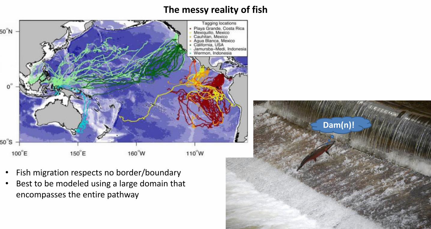
The messy reality of fish

Dam(n)!

5

• Fish migration respects no border/boundary• Best to be modeled using a large domain that

encompasses the entire pathway

Can we build a baroclinic

unstructured-grid model from river to

ocean?

Baroclinic circulation is still mostly done using SG models with grid nesting

UG models: “complex geometry, simple flow”

SG models: “simple geometry, complex flow”

The great disappearing act of UG models

500m

Coos Bay

50km

500m

500m

Grays Harbor

Columbia River

Tsunami

Storm surge(Westerink et al. 2008)

UG models are ‘natural’ for multi-scale processes…. but so far are mostly used for barotropicprocesses

(Oey et al. 2013)

6

Progress in the large-scale UG modeling…

Skamarock et al. (2012)

MPAS o on Spherical Centroidal Voronoi Tessellations (SCVT),

Arakawa-C grid (orthogonal), globalo FV formulation (vector invariant)o Mostly free of spurious numerical ‘modes’o Ocean, seaice, landice, atmosphere…

FESOM2 o on hybrid triangle-quadso FV formulation

ICONo on orthogonal triangleso FV formulation

However, significant challenges remain from deep ocean into shallow waters o Part of these challenges are due to physics (e.g., scale

differences =>different parameterizations)o Scale-aware parameterization is an active research areao However, underlying numerics are lacking even if we

restrict ourselves to hydrostatic regime

7

MPAS-OI: a nearshore component of global MPAS-Ocean Funded by US Dept. of Energy to bridge the

gap between global ocean model and rivers o Both SCHISM and MPAS-OI will be fully

coupled to MPAS-O Formulation based on the subgrid, FV solver of

UnTRIM (Casulli 2009), but with MPAS’ approach for conservation of mass, energy and potential vorticity (Thuburn et al. 2009)

The core is a semi-implicit, nonlinear solver for coupled continuity and momentum equationo The convergence of the nonlinear solver

is always guaranteedo Enables mass conservative wetting and

drying with any time step used Subgrid capability for better representation of

bathymetry

MPAS-OI: inundation test on a parabolic bowl

Rotated symmetric bowl to test robustness

Days

Vo

lum

e r

atio

Analytical

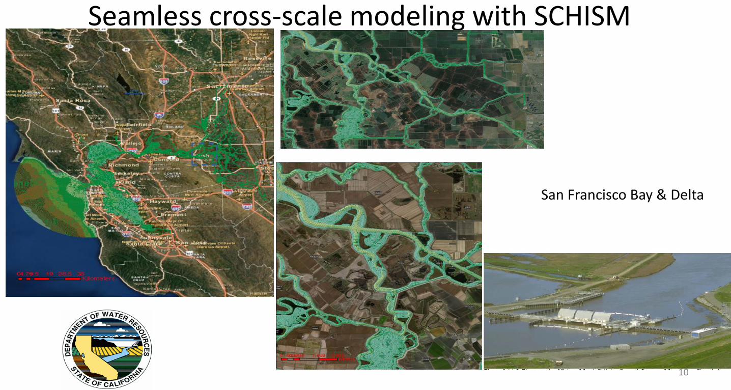
Seamless cross-scale modeling with SCHISM

10

San Francisco Bay & Delta

Seamless cross-scale modeling with SCHISM

11

• Bridge crossings on James River, Chesapeake Bay• Bridge pilings of 1-2m in diameter• ~1840 pilings located in the middle of salt

intrusion path

SCHISM: Semi-implicit Cross-scale Hydroscience Integrated System Model

A derivative product of SELFE v3.1, distributed with open-source Apache v2 license

Substantial differences now exist between the two models

Free svn access to release branch for general public

Galerkin finite-element and finite-volume approach: generic unstructured triangular gridsELCIRC (Zhang et al. 2005), UnTRIM (Casulli 1990; 2010), SUNTANS (Fringer 2006): finite-difference/volume approach orthogonal grid

Hydrostatic or non-hydrostatic options

Semi-implicit time stepping: no mode splitting large time step and no splitting errors

Eulerian-Lagrangian method (ELM) for momentum advection more efficiency & robustness

Major differences from SELFE v3.1

Apache license

Mixed grids (tri-quads)

LSC2 vertical grid (Zhang et al. 2015)

Implicit TVD transport (TVD2) & WENO3

Higher-order ELM with ELAD

Bi-harmonic viscosity

Eddying regime (Zhang et al. 2016)

visit schism.wiki

SELF

ESC

HIS

M

12

c/o Karinna Nunez 13

Why SCHISM?

Major differentiators from peer models

No bathymetry smoothing or manipulation necessary: faithful representation of bathymetry is key in nearshore regime

Implicit FE solvers superior stability very tolerant of bad-quality meshes (at least in non-eddying regime)

Accurate yet efficient: implicit + low inherent numerical dissipation; flexible gridding system

Need for grid nesting is minimized

Well-benchmarked; certified inundation scheme for wetting and drying (NTHMP)

Fully parallelized with domain decomposition (MPI+openMP) with strong scaling (via PETSc solver)

Operationally tested and proven (DWR, NOAA, CWB …)

Open source, with wider community support (210+ registered user groups)14

Underlying numerics matter! Explicit ‘mode-splitting’ models

Solves the hydrostatic equations in external and internal mode separately (splitting errors)

Easy to implement (with possible exception of filters), and well understood

99% of the existing models

Subject to CFL constraints (severe in shallow water)

Structured and unstructured grids

Excellent parallel scaling

Implicit models: the cross-scale models?

Solve the HS equations in one time step (no mode splitting errors)

Difficult to formulate (and parallelize)

No CFL constraints; superior stability

Mostly on unstructured grids

Parallel scaling not as good

Numerical diffusion needs to be controlled

15

UnTRIM

SHYFEM

SUNTANS ELCIRC

SELFE/SCHISM

ECOM-si

Underlying bathymetry matters even more: respect the bathymetry!

Faithful representation of bathymetry is of fundamental importance especially in nearshoreTwo types of bathymetric errors

Type I: Finite grid resolution; bathymetry survey errors; smoothing of DEM for unresolved sub-grid scales - not a convergence issueType II: Smoothing or other manipulations (e.g. as in terrain-following coordinate models) - a divergence error as refining grid generally makes it worse!

SCHISM’s representation of the bathymetry is piece-wise linearVery skew elements are allowed in non-eddying regime; implicit scheme guarantees stability

Facilitates feature-tracking in grid generation There is no need for bathymetry smoothing to stabilize the model

16

Detrimental effects of bathymetry smoothing

Cross-channel transect with deep center channel

Volume is conserved during smoothing

Smoothing in a critical region where the center

channel constricts and bends, with multi-channel

configurations

17

Larger sub-tidal volume flux

Smaller amplitude of tidal volume flux:

smoothed = 79% original

Focusing on the cross transect on

the west part of the main stem, the

smoothing effects include:

More salt, about +1 PSU in the smoothed

region, 2-3 PSU upstream

CB5.4

Vertic

al d

iffusiv

ity [lo

g10

(m2

s-1)]

Time averaged

Original

Smoothed

The effect of smoothing on turbulent mixing: less

mixing overall and less contrast between shoal

and channel

Bathymetry smoothing effectively masks true numerical dissipation!

18

Sensitivity test 1: mid-Bay smoothing

Cross-sectional salinity distribution

Original

bathymetry

Smoothed

bathymetrySaltier

Less channel-shoal difference

19

Sensitivity test 2: whole-Bay smoothing

Stratification

Original

Bathymetry

Smoothed

Bathymetry

More stratified due to stronger gravitational circulation

Channelized intrusionUniform intrusion

20

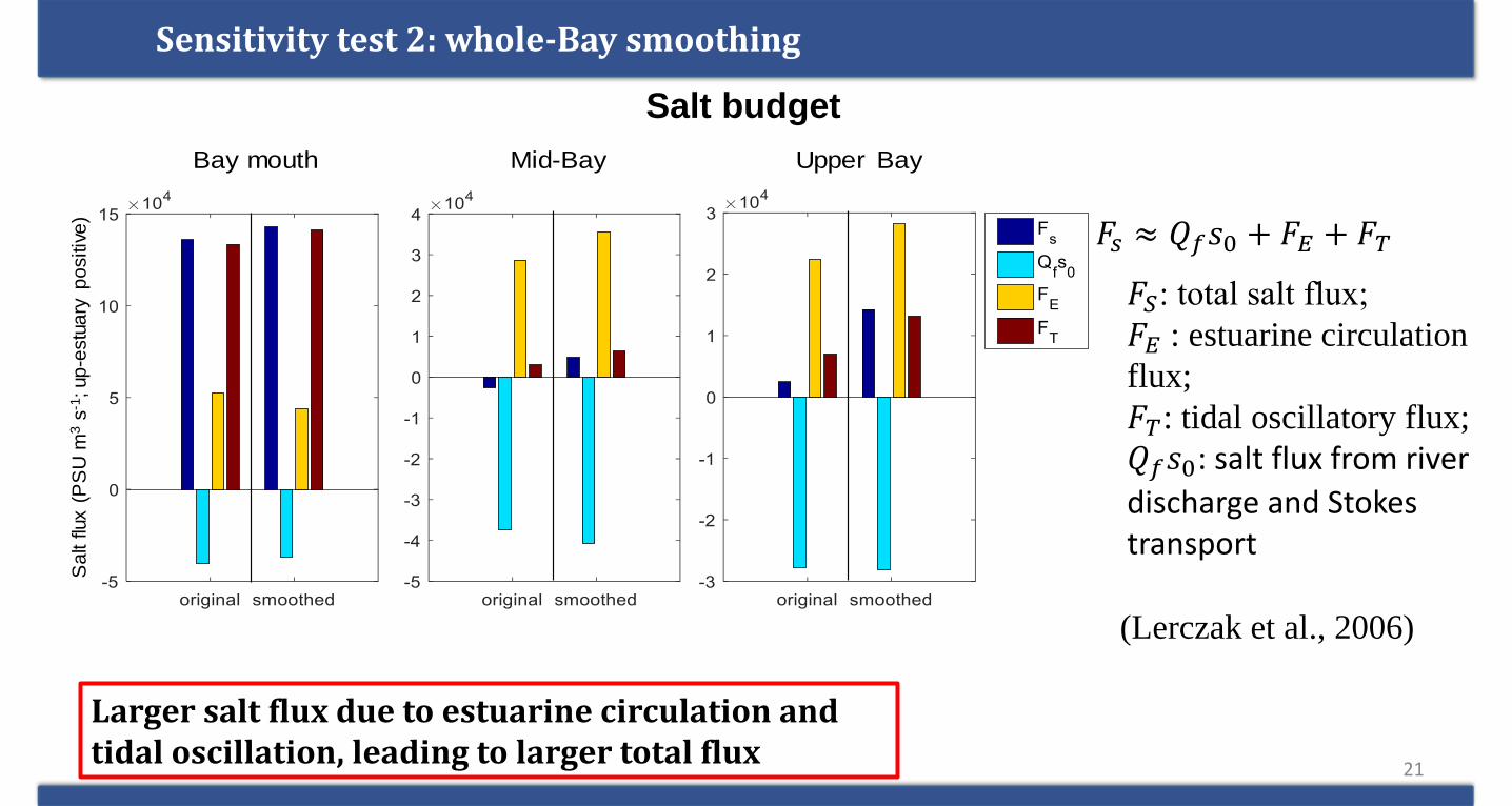
Sensitivity test 2: whole-Bay smoothing

Bay mouth Lower Bay Mid-Bay Upper mid-Bay Upper BayBay mouth Lower Bay Mid-Bay Upper mid-Bay Upper BayBay mouth Lower Bay Mid-Bay Upper mid-Bay Upper BayBay mouth Lower Bay Mid-Bay Upper mid-Bay Upper Bay

Sa

lt flu

x (P

SU

m3

s-1

; up

-estu

ary

p

ositiv

e)

Salt budget

𝐹𝑆: total salt flux;𝐹𝐸 : estuarine circulation

flux;

𝐹𝑇: tidal oscillatory flux;

𝑄𝑓𝑠0: salt flux from river

discharge and Stokes transport

Larger salt flux due to estuarine circulation and tidal oscillation, leading to larger total flux

𝐹𝑠 ≈ 𝑄𝑓𝑠0 + 𝐹𝐸 + 𝐹𝑇

(Lerczak et al., 2006)

21

Grid generation in SCHISM: less numerics, more physics

Channel Shoal

Tidal range

Skew elements

Channel representation

22

How skew can you go??

23

Extreme case #1: skew elements are a boon in nearshore applications

In the non-eddying regime, skew elements can save a lot of computational cost!Fringing marshes need fine resolution (1m cross, 15m along)The implicit FE formulation in SCHISM makes it very tolerant of ‘bad’ meshesFully coupled SCHISM-SED-WWM-Marsh model runs stably on this type of meshesMarsh migration in 30 years, with 4mm/yr sea-level riseFlow/wave impedance by marsh vegetation is incorporated in the implicit solver

Smooth-transitioning grid would be 10x larger!

Fringing marshes

24

Applications c/o: SCHISM users

5

2

1

3 4

10

6

8

7

11

12 13

9 14

15

16

1 23

45

10

6

78911

1213

14

1516

25

Columbia River Forecast

http://tidesandcurrents.noaa.gov/ofs/creofs/creofs.htmlNOAA COOPS 26

San Francisco Bay & Delta

27

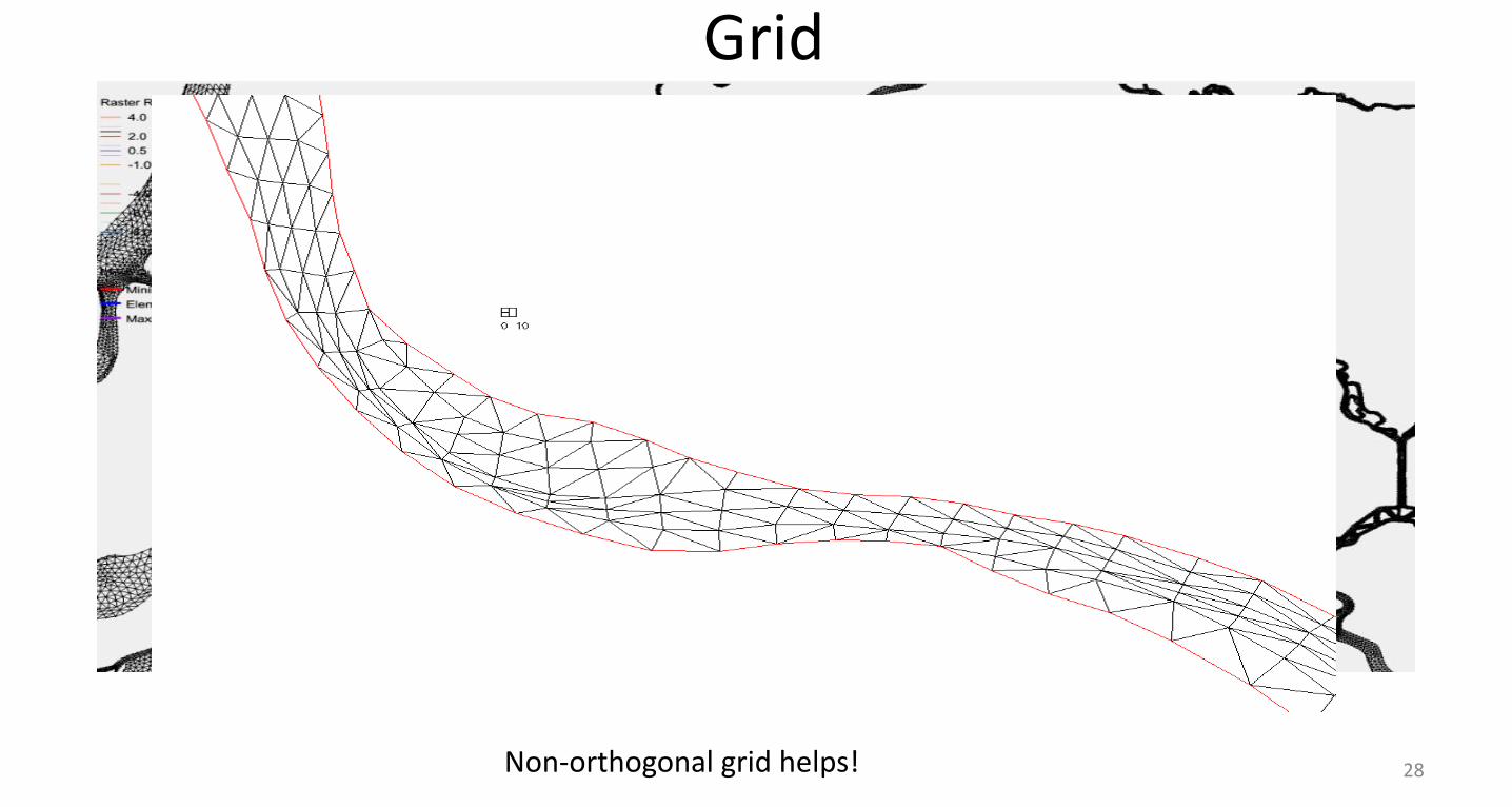
Grid

Non-orthogonal grid helps! 28

Extend the model to large scale: from estuary to shelf and beyond

29

Main motivation is the errors & uncertainties at the ocean boundary often strongly influence the solution interiorNumerical challenges for cross-scale processes

Efficiency: mainly related to higher-order transport solver (explicit TVD)Performance in eddying regime (baroclinic instability): PGE, spurious numerical modes/mixing….

UG models make some old issues more urgentGrid transition in SG models is always smoothCoarser resolution in SG models masks issues with steep bathymetry

Strategy (for eddying and non-eddying regimes)Reduce inherent numerical dissipation by combining the FE (dispersive) and implicit scheme (diffusive)Make the higher-order transport solver implicit (in the vertical), without introducing excessive numerical diffusionMake the grid system flexible (good for shallow depths also!)Rework momentum advection and viscosity schemes to control dissipation

Model polymorphism

1

2

P

QR

A

B

Zhang et al. (2015)30

Polymorphism in action

S(PSU)

S(PSU)

0

0.15

The stratified Bay is represented by 3D gridThe shallow Delta region is mostly represented as 2DThere are only ~10 layers on average

31

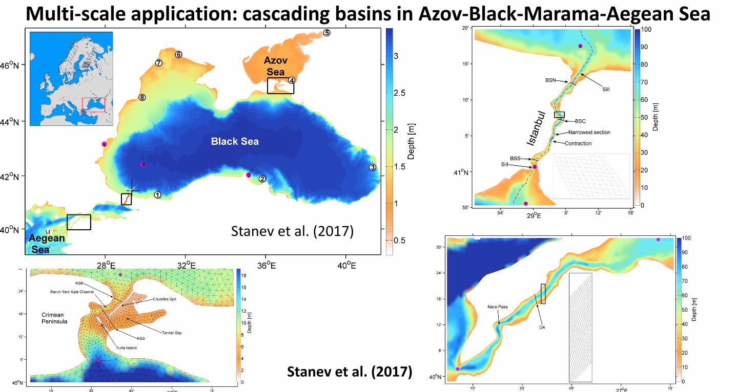
Multi-scale application: cascading basins in Azov-Black-Marama-Aegean Sea

Stanev et al. (2017)

32Stanev et al. (2017)

An extreme case…

Bosphorus Strait Marmara Sea Black Sea

Either Z or terrain-following grid will have issues here…

Bosphorus Strait

33

Black Sea: eddying activity

08-Oct-2008

12-Nov-2008

22-Jan-2009

Relative vorticity/fSSTSSH

Stanev et al. (2017) 34

Black Sea: overflow

Salinity

West East South North

Distance along transect (km)

South North South North

‘Negative plume’

(Bosphorous) (Black Sea)

Stanev et al. (2017) 35

Multi-scale application: Northwestern Pacific around TaiwanModel set-up

Horizontal grid: 480K nodes, 960K elements. Quasi-uniform resolution in open seas (5-9km), 100-200m around Taiwan, 50m nearshore, 5m min resolution (in ports/harbors)Vertical grid: LSC2, max 41 layers (@10km depth), average 29 layersNo bathymetry smoothing/clipping (c/o LSC2)Dt=120s, bi-harmonic viscosityI.C. and B.C. from HYCOM

Model performance: 120x RT on 480 Intel cores

Bathymetry

Zheng et al. (2006)

Yu et al. (2017)36

Large-scale skill: Kuroshio(Zhang et al. 2017)

SST SSS

SSH

37

Nearshore skillM2

M2 amplitude

M2 phase

Stations

DATA HYCOM SCHISM_tide SCHISM_notide

Days after April 1, 2013

T (o

C)

1

2

3

4

5

6

Yu et al. (2017)38

Importance of higher-order scheme in eddying regime: Gulf Stream meandering

3rd order WENO2nd order TVD

SST(oC) SST(oC)

Grid resolution: 2~7 km; 388K nodes and 766K elements; 27 LSC2 vertical levels on

average

Time step=150 seconds

No bathymetry smoothing 39

SCHISM web

40

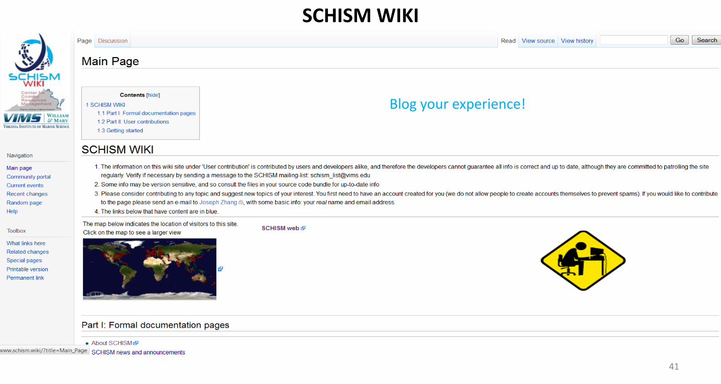
SCHISM WIKI

41

Blog your experience!

Summary: how far can we push the cross-scale model?

We have made good progress on seamless cross-scale modelling during the past 17 yearsSeamless cross-scale modeling can be effectively done with unstructured grids and

implicit time steppingBesides accuracy consideration, efficiency, flexibility and robustness are also important factors in this endeavorBalance between lower- and higher-order schemes is importantA seamless platform with 1D/2D/3D capability leads to efficiencySCHISM is well demonstrated for nearshore and estuarine applicationsWe have extended SCHISM to large scale, in order to better handle the boundary condition

How far can we go?Nearshore: upstream rivers/creeksOffshore: regional scaleUltimate goal is to build a model that covers ocean-shelf-estuary-river-creek system without nesting (or at least minimize its use)