GLOBEFISH RESEARCH PROGRAMME

Food and Agriculture Organization of the United NationsFishery Industries Division

Viale delle Terme di Caracalla00100 Rome, Italy

Tel.: +39 06 5705 5074Fax: +39 06 5705 5188

www.globefish.org

Seafood Price Indices

Volume 78

SEAFOOD PRICE INDICES

by

Sigbjorn Tveteras Consultant, GLOBEFISH

April 2005

The GLOBEFISH Research Programme is an activity initiated by FAO's Fishery Industries Division, Rome, Italy and financed jointly by: - NMFS (National Marine Fisheries Service), Washington, DC, USA - FROM, Ministerio de Agricultura, Pesca y Alimentación, Madrid, Spain - Ministry of Food, Agriculture and Fisheries, Copenhagen, Denmark - European Commission, Directorate General for Fisheries, Brussels, EU - Norwegian Seafood Export Council, Tromsoe, Norway - OFIMER (Office National Interprofessionnel des Produits de la Mer et de l’Aquaculture), Paris, France - SHILAT, Iranian Fisheries, Iran - VASEP, Viet Nam Association of Seafood Exporters and Producers, Viet Nam

Food and Agriculture Organization of the United Nations, GLOBEFISH, Fishery Industries Division Viale delle Terme di Caracalla, 00100 Rome, Italy – Tel.: (39) 06570 56313/06570 54759 - E-mail:

GLOBEFISH@fao.org - Fax: (39) 0657055188 – http//:www.globefish.org

The designation employed and the presentation of material in this publication do not imply the expression of any opinion whatsoever on the part of the Food and Agriculture Organization of the United Nations concerning the legal status of any country, territory, city or area or of its authorities, or concerning the delimitation of its frontiers or boundaries.

Photographs on cover page courtesy of Norwegian Seafood Export Council

Tveteras, S. Seafood Price Indices GLOBEFISH Research Programme, Vol.78. Rome, FAO. 2005. 44p.

Due to the different species, commodities and preservation methods it was considered difficult to give indications in general on the development of prices for seafood. The import price indices developed in this report are based on unit values and it is shown that unit values reflect closely the development of actual prices. The reason why unit values are used is described and a detailed description of the scientific base for the construction of indices is given. The result shows that prices for the majority of fish products remain either stable or mostly decreased.

ISSN 1014-9546

All rights reserved. No part of this publication may be reproduced, stored in a retrieval system, or transmitted in any means, electronic, mechanical, photocopying or otherwise, without the prior permission of the copyright owner. Applications for such permission, with a statement of the purpose and extent of the reproduction, should be addressed to the Director, Information Division, Food and Agriculture Organization of the United Nations, Viale delle Terme di Caracalla, 00100 Rome, Italy.

© FAO 2005

iii

TABLE OF CONTENTS 1 INTRODUCTION ................................................................................................................. 1 2 METHODOLOGY ................................................................................................................ 4 2.1 Price Index Theory ........................................................................................................... 4 2.2 Index Formulas................................................................................................................. 5 2.3 Base Period....................................................................................................................... 6 2.4 Missing Observations....................................................................................................... 6 2.5 Seasonal Movements........................................................................................................ 7 2.6 Currency ........................................................................................................................... 7 2.7 Revisions in Trade Statistics’ Product Categories ........................................................... 7 2.8 Market Integration and Aggregation ................................................................................ 7 3 EMPIRICAL EVIDENCE – THE FAO SEAFOOD IMPORT PRICE INDICES ....... 11 3.1 . Frozen Shrimp ................................................................................................................ 11 3.2 . Frozen Groundfish.......................................................................................................... 13 3.3 . Canned Tuna .................................................................................................................. 15 3.4 . Fresh Salmon.................................................................................................................. 17 4 PERFORMANCE OF THE FAO SEAFOOD IMPORT PRICE INDICES ................. 20 5 SEAFOOD IMPORT PRICE TRENDS............................................................................ 23 5.1 . Price Trends for Aquaculture Versus Wild-caught Seafood Products ........................... 23 5.2 . Seafood Versus Meat Prices........................................................................................... 26 5.3 . Import Seafood Prices Versus Consumer Prices............................................................ 28 Reference................................................................................................................................... 30 6 APPENDICES...................................................................................................................... 31 6.1 Johansen Multivariate Cointegration............................................................................... 31 6.2 Testing for Leading Prices............................................................................................... 32 6.3 Construction of a Shrimp Price Index ............................................................................. 33 6.4 Actual Prices from Different Sources as Reported and Collected in the GLOBEFISH Databank and the GLOBEFISH Commodity Updates ............................. 38 FIGURES AND TABLES Figure 1.1 Seafood Exports from Developing and Developed Countries, 1976 to 2002

(FAO) Figure 1.2. Seafood import value to the EU and USA, 1976-2002 (FAO) Figure 3.1. Apparent Shrimp Consumption in EU and USA (FAO Fishstat Database) Figure 3.2. FAO Shrimp Price Indices for EU and USA (Base: 1997-1999 = 100) Figure 3.3. Global Pollock, Cod, Hake, Haddock, and Saithe Catches (FAO Fishstat

Database)

iv

Figure 3.4. Apparent Consumption of Frozen Groundfish in EU and USA (FAO Fishstat Database)

Figure 3.5. FAO Price Indices for Cod, Frozen Fillet, EU and USA (Base: 1997- 1999 = 100)

Figure 3.6. FAO Price Indices for Alaska Pollock and Saithe, Frozen Fillet, EU and USA (Base: 1997-1999 = 100)

Figure 3.7. Global Tuna Catches By Species (FAO Fishstat Database) Figure 3.8. EU Tuna Imports by Product Group (FAO Fishstat Database) Figure 3.9. US Tuna Imports by Product Group (FAO Fishstat Database) Figure 3.10. FAO Price Indices for Canned Tuna, EU and USA (Base: 1997-1999 = 100) Figure 3.11. Salmon Aquaculture and Capture Fisheries Production (FAO Fishstat Database) Figure 3.12. EU Salmon Imports by Major Product Groups (FAO Fishstat Database) Figure 3.13. US Salmon Imports by Major Product Groups (FAO Fishstat Database) Figure 3.14. FAO Price Indices for Salmon, Fresh Whole and Fillet, EU and USA

(Base: 1997-1999 = 100) Figure 4.1. Shrimp Price Indices Based on Unit Values (black) and Prices (grey) Figure 4.2. Cod Price Indices Based on Unit Values (black) and Prices (grey) Figure 4.3. Alaska Pollock Price Indices Based on Unit Values (black) and Prices (grey) Figure 4.4. Tuna Price Indices Based on Unit Values (black) and Prices (grey) Figure 5.1. US Import Price Trends for Frozen Groundfish Fillets, Frozen Shrimp and Fresh

Salmon Figure 5.2. EU Import Price Trends for Frozen Groundfish Fillets, Frozen Shrimp and Fresh

Salmon Figure 5.3. US Imports of Atlantic Cod and Alaska Pollock Frozen Fillets (NMFS) Figure 5.4. US Import Price Trends for Fresh and Frozen Tilapia Fillets and Frozen

Groundfish Fillets Figure 5.5. Price Trends for US Imports of Frozen Shrimp by Size Grade Figure 5.6. Price Trends for Meat Products and Frozen Groundfish Figure 5.7. Price Trends for Poultry, Pig, Salmon and Shrimp Figure 5.8. CPI-adjusted US Import Price Trends for Frozen Groundfish Fillets, Frozen

Shrimp and Fresh Salmon Figure A.1. The NMFS Website for Monthly Trade Statistics Figure A.2 The Shrimp Statistics As a Raw Data Sheet Figure A.3. The Shrimp Statistics in a Pivot Sheet Figure A.4. The Shrimp Statistics from the Pivot Sheet -Pasted into a New Sheet Figure A.5. The Shrimp Price Index Figure A.6. The Shrimp Price Index Table 2.1. Some Commodity Used Index Measures

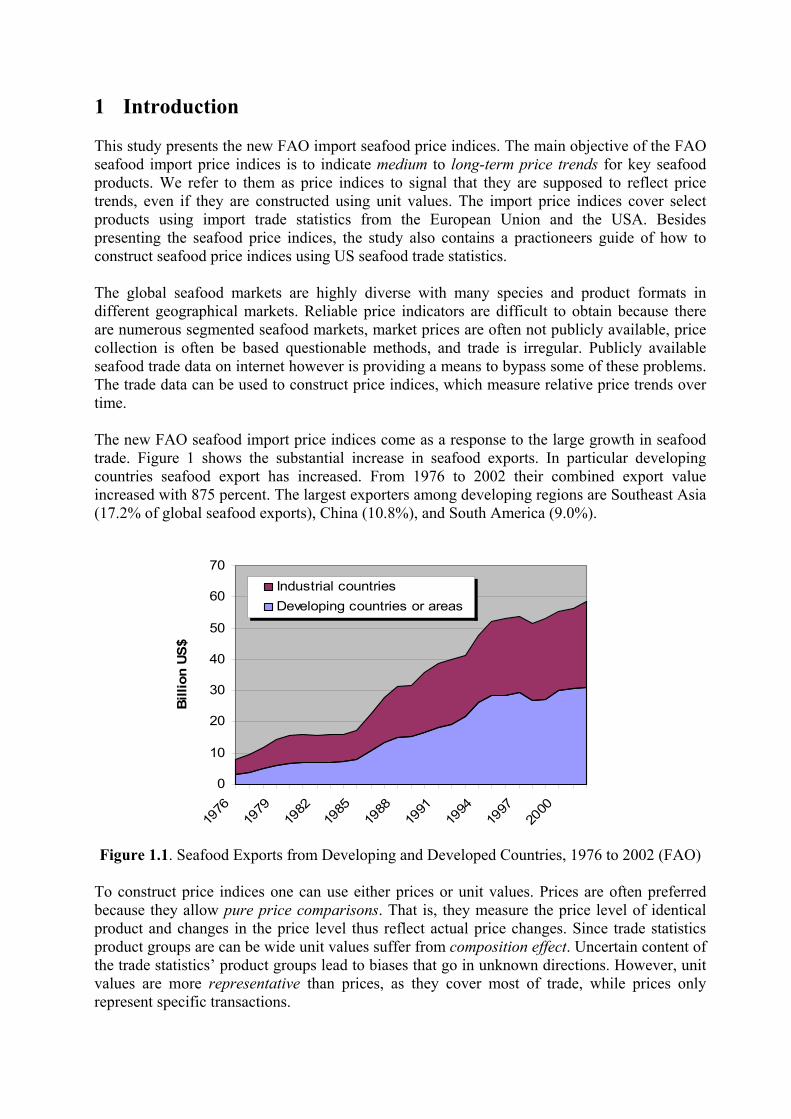
1 Introduction This study presents the new FAO import seafood price indices. The main objective of the FAO seafood import price indices is to indicate medium to long-term price trends for key seafood products. We refer to them as price indices to signal that they are supposed to reflect price trends, even if they are constructed using unit values. The import price indices cover select products using import trade statistics from the European Union and the USA. Besides presenting the seafood price indices, the study also contains a practioneers guide of how to construct seafood price indices using US seafood trade statistics. The global seafood markets are highly diverse with many species and product formats in different geographical markets. Reliable price indicators are difficult to obtain because there are numerous segmented seafood markets, market prices are often not publicly available, price collection is often be based questionable methods, and trade is irregular. Publicly available seafood trade data on internet however is providing a means to bypass some of these problems. The trade data can be used to construct price indices, which measure relative price trends over time. The new FAO seafood import price indices come as a response to the large growth in seafood trade. Figure 1 shows the substantial increase in seafood exports. In particular developing countries seafood export has increased. From 1976 to 2002 their combined export value increased with 875 percent. The largest exporters among developing regions are Southeast Asia (17.2% of global seafood exports), China (10.8%), and South America (9.0%).

0

10

20

30

40

50

60

70

1976

1979

1982

1985

1988

1991

1994

1997

2000

Billi

on U

S$

Industrial countriesDeveloping countries or areas

Figure 1.1. Seafood Exports from Developing and Developed Countries, 1976 to 2002 (FAO)

To construct price indices one can use either prices or unit values. Prices are often preferred because they allow pure price comparisons. That is, they measure the price level of identical product and changes in the price level thus reflect actual price changes. Since trade statistics product groups are can be wide unit values suffer from composition effect. Uncertain content of the trade statistics’ product groups lead to biases that go in unknown directions. However, unit values are more representative than prices, as they cover most of trade, while prices only represent specific transactions.

2

The problems with available price series are several. The most serious problem is the time span and discontinuities. Most price series available to us have a shorter span than ten years and usually many observations are missing. Further, no transacted quantities are associated with the prices, so it is uncertain whether high or low price levels are due to general market movements or due to large or small volumes associated with the specific transactions. Finally, quoted prices from key markets and key exporting countries are missing, making the alternative prices less representative for the task as a price index. It is controversial to use unit values as a proxy for prices. For example the FAO seafood import price indices will unavoidably suffer from composition effects. Within a product group there might be several quality grades, size grades, product formats, and seafood species. The severity of the composition effects depends on how wide is the relevant product categories in the trade statistics. Another issue is the time lag from a transaction is made to a product physically crosses the border or is reported to the authorities. The time lag implies that monthly trade statistics includes transactions from preceding weeks and months. These aggregation issues can mask the ‘true’ market price trend. We have decided to report monthly indices despite the time lag aggregation issue, as the monthly variation may still contain useful information. The price indices are nevertheless better understood as reflecting quarterly and annual price trends. Most of the FAO seafood import price indices consist of a single product category in order to avoid further aggregation biases besides the composition and temporal effects. Overall, the biases are judged to be within acceptable limits for FAO’s purposes, partly because the product formats of widely traded seafood products have remained similar over the years and partly because the main objective is to represent long-term market trends. Fresh salmon, frozen shrimp, frozen cod and canned tuna products in the EU and the US markets are targeted for the price indices. Most indices start from January 1989 or early 1990s. The selection covers two of the largest seafood markets (Japanese seafood imports are larger than the US in value, but is disregarded because of less accessible internet databases for trade statistics). Likewise, the products are in terms of value among the most important in international seafood trade. There are clear advantages of focusing on such products: (1) because of their importance in seafood trade, they can be indicative for the price of a number of related seafood products, (2) more reliable and consistent data are available for these products compared with many other seafood products, and (3) by limiting the selection to a few key products and key markets the work will be kept at manageable proportions. The FAO seafood price indices are representative for a limited number of species and markets. Even if it would be desirable to cover more of seafood trade, the extra workload is currently outside the scope of FAO. Thus we have decided to present a manual, of sorts, on how to construct price indices using seafood trade data, to assist those interested in constructing price indices for other products and markets.

3

0

5

10

15

20

25

1976

1978

1980

1982

1984

1986

1988

1990

1992

1994

1996

1998

2000

2002

Billi

on U

S$

in E

U

0

2

4

6

8

10

12

Billi

on U

S$ in

USA

European UnionUSA

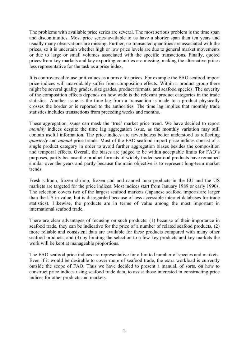
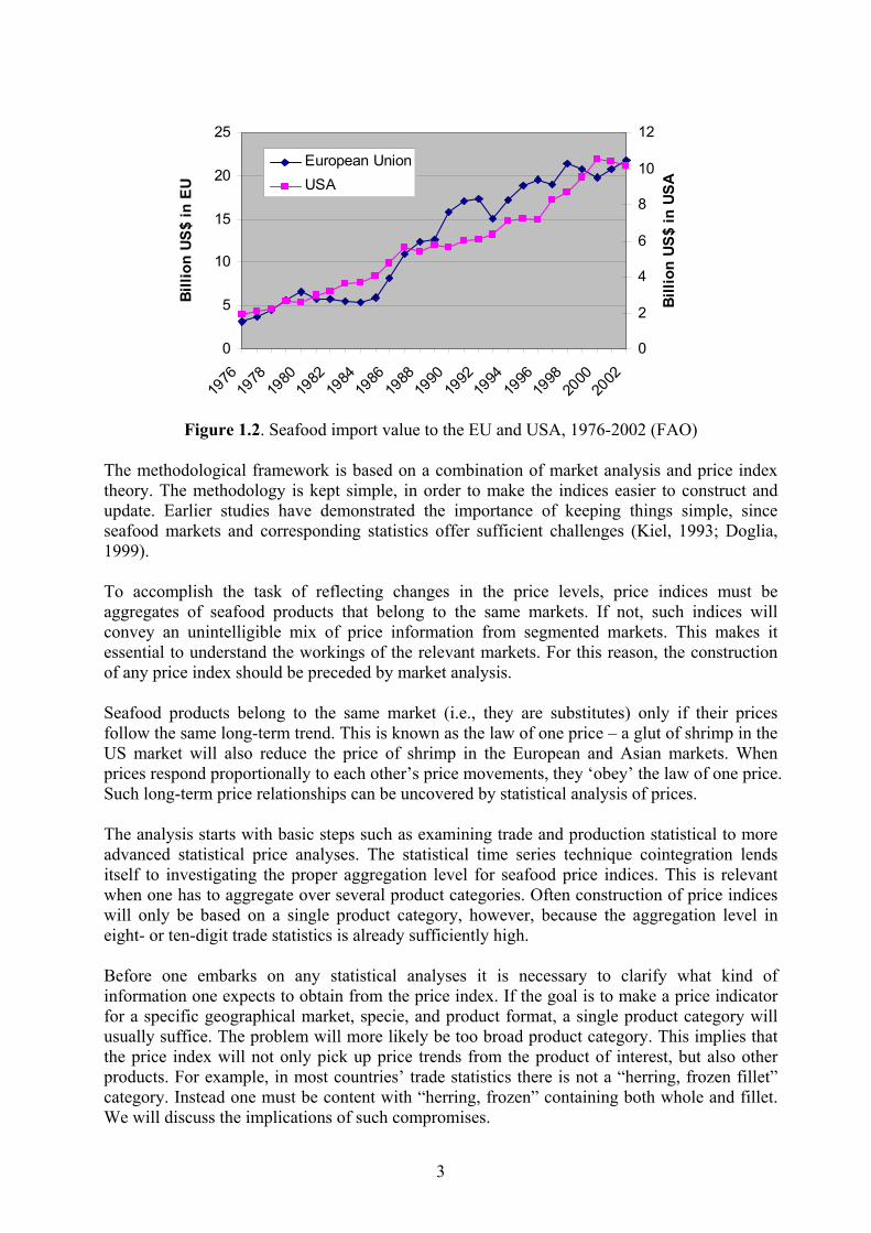
Figure 1.2. Seafood import value to the EU and USA, 1976-2002 (FAO)

The methodological framework is based on a combination of market analysis and price index theory. The methodology is kept simple, in order to make the indices easier to construct and update. Earlier studies have demonstrated the importance of keeping things simple, since seafood markets and corresponding statistics offer sufficient challenges (Kiel, 1993; Doglia, 1999). To accomplish the task of reflecting changes in the price levels, price indices must be aggregates of seafood products that belong to the same markets. If not, such indices will convey an unintelligible mix of price information from segmented markets. This makes it essential to understand the workings of the relevant markets. For this reason, the construction of any price index should be preceded by market analysis. Seafood products belong to the same market (i.e., they are substitutes) only if their prices follow the same long-term trend. This is known as the law of one price – a glut of shrimp in the US market will also reduce the price of shrimp in the European and Asian markets. When prices respond proportionally to each other’s price movements, they ‘obey’ the law of one price. Such long-term price relationships can be uncovered by statistical analysis of prices. The analysis starts with basic steps such as examining trade and production statistical to more advanced statistical price analyses. The statistical time series technique cointegration lends itself to investigating the proper aggregation level for seafood price indices. This is relevant when one has to aggregate over several product categories. Often construction of price indices will only be based on a single product category, however, because the aggregation level in eight- or ten-digit trade statistics is already sufficiently high. Before one embarks on any statistical analyses it is necessary to clarify what kind of information one expects to obtain from the price index. If the goal is to make a price indicator for a specific geographical market, specie, and product format, a single product category will usually suffice. The problem will more likely be too broad product category. This implies that the price index will not only pick up price trends from the product of interest, but also other products. For example, in most countries’ trade statistics there is not a “herring, frozen fillet” category. Instead one must be content with “herring, frozen” containing both whole and fillet. We will discuss the implications of such compromises.

4

2 Methodology This section presents the methodology for the new FAO seafood import price indices. The first subsections deals with index number theory, which deals with issues like how to represent many prices with one index, choice of base period, and missing observations. Products or geographical markets for identical products should only be represented by a common price index if they belong in the same market. The last section deals with economic theory, which can guide us to choose a proper aggregation level. This is in particular when using price data, because they are much more disaggregated than trade statistics. Products that belong to the same market can be aggregated into one price index. Since seafood markets are diverse we use some space on this subject with extensions in the Appendices A1 and A2. 2.1 Price Index Theory A price index is a comparative or relative measure over time. Usually, it is two periods compared with each other.1 The two main uses of a price index are either as a deflator or as a price level measurement. Here the price index is used as a measurement of the import price level for seafood. When constructing a price index one encounters the index number problem, which, simply put, is how to represent a large number of prices and quantities with only one price index. This question is particular relevant for seafood markets where the product diversity is formidable. Diewert formulates the index number problem formally (1987),

(2.1) ∑=

⋅≡⋅=N

iitittttt qpqpQP

1 for .,...,1 Tt =

tP is the price index for period t (or unit i) and tQ is the corresponding quantity index. tP is

supposed to be representative of all of the prices itp , Ni ,...,1= in some sense while tQ is supposed to be similarly representative of all of the quantities itq , Ni ,...,1= . In what precise sense tP and tQ represent the individual prices and quantities is not immediately evident and it is this ambiguity that leads to different approaches to index number theory. Representativeness and pure price comparison are two sought after characteristics of a price index. Representiativeness refers to how typical is the price determination process for the market. For example, if prices are collected from a specific producer there may be many characteristics of the producer and the transactions which are not representative for the ‘average’ or typical transactions in the market. The advantage of trade statistics is that it covers the majority of transactions in trade, export and import (given that trade flows are reported to the authorities). Pure price comparison, on the other hand, is concerned with identifying the conditions for transactions that are similar (except for time or location). A pure price comparison in seafood trade would be, say, if you compared exactly the same product, e.g., black tiger shrimps, frozen, tail on, 21/60 count per pound, origin Thailand, 4 pound packs, equivalent traded volume in the same location, etc. So in addition to the product specifications 1 As most of the price indices use only a single product category in import trade statistics (i.e., a single variable), some may find it more useful to express the product with the price level instead of as a price index, as is done here.

5

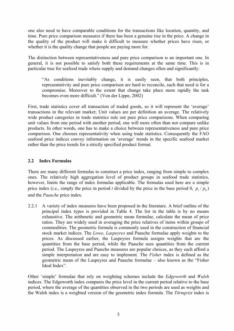
one also need to have comparable conditions for the transactions like location, quantity, and time. Pure price comparison measures if there has been a genuine rise in the price. A change in the quality of the product will make it difficult to measure whether prices have risen, or whether it is the quality change that people are paying more for. The distinction between representativeness and pure price comparison is an important one. In general, it is not possible to satisfy both these requirements at the same time. This is in particular true for seafood trade where supply and demand changes often and significantly: “As conditions inevitably change, it is easily seen, that both principles, representativity and pure price comparison are hard to reconcile, such that need is for a compromise. Moreover to the extent that change take place more rapidly the task becomes even more difficult.” (Von der Lippe, 2002) First, trade statistics cover all transaction of traded goods, so it will represent the ‘average’ transactions in the relevant market; Unit values are per definition an average. The relatively wide product categories in trade statistics rule out pure price comparisons. When comparing unit values from one period with another period, one will more often than not compare unlike products. In other words, one has to make a choice between representativeness and pure price comparison. One chooses representativity when using trade statistics. Consequently the FAO seafood price indices convey information on ‘average’ trends in the specific seafood market rather than the price trends for a strictly specified product format. 2.2 Index Formulas There are many different formulas to construct a price index, ranging from simple to complex ones. The relatively high aggregation level of product groups in seafood trade statistics, however, limits the range of index formulas applicable. The formulas used here are a simple price index (i.e., simply the price in period t divided by the price in the base period 0, 0/ ppt ) and the Paasche price index. 2.2.1 A variety of index measures have been proposed in the literature. A brief outline of the

principal index types is provided in Table 4. The list in the table is by no means exhaustive. The arithmetic and geometric mean formulae, calculate the mean of price ratios. They are widely used in averaging the price relatives of items within groups of commodities. The geometric formula is commonly used in the construction of financial stock market indices. The Lowe, Laspeyres and Paasche formulae apply weights to the prices. As discussed earlier, the Laspeyres formula assigns weights that are the quantities from the base period, while the Paasche uses quantities from the current period. The Laspeyres and Paasche measures are popular choices, as they each afford a simple interpretation and are easy to implement. The Fisher index is defined as the geometric mean of the Laspeyres and Paasche formulae – also known as the “Fisher Ideal Index”.

Other ‘simple’ formulae that rely on weighting schemes include the Edgeworth and Walsh indices. The Edgeworth index compares the price level in the current period relative to the base period, where the average of the quantities observed in the two periods are used as weights and the Walsh index is a weighted version of the geometric index formula. The Törnqvist index is

6

similar to the Walsh index, except that the value shares of each commodity in the base and current periods are averaged. Table 2.1: Some Commonly Used Index Measures Index Type Index Formula

Arithmetic Mean ( )01 /it i

i

p pn∑

Laspeyres 0 0 0/it i i ii i

p q p q∑ ∑

Paasche 0/it it i iti i

p q p q∑ ∑

Fisher 1/ 2

0 0 0 0/ /it i i i it it i iti i i i

p q p q p q p q ∑ ∑ ∑ ∑

Note: The following notation applies to each formula. For commodity i (i =1,…n) p is the price, q is the weight applied to the price, and the subscripts t and 0 refer to the current time period and base period respectively. 2.3 Base Period The choice of base year or base period can have great impact on the behaviour of the price index, as it determines the relative weighting scheme among the products. The base period should be a normal year in respect of production and trade. The base year should be as recent as possible so that by the time the revised series is released it has not outlived its utility. It is common practice to rebase Laspeyres indices after a few years, say, every three years or every 5 years. The time for the reweighting can exactly be defined by running a Laspeyres index in parallel to a Paasche index and drawing current comparisons between them both: when their divergence becomes to large, the Lasperres type has to be rebased. Rebasing means repetition of a large part of the work that to be done before an index run is started for the first time (von der Lippe, 1985; UN, 1977). A rebased Laspeyres run will show a price increase smaller than the old run, if prices and quantities are negatively correlated, or vice versa (Allen, 1976, pp 27-33, 156-163). Therefore the often mentioned argument that a Paasche index is more difficult to interpret do not hold. It also requires less work to update the index. 2.4 Missing Observations Index numbers are supposed to show continuous information about movements of a set of variables. Situations often arise when data are not available at either a point in time or over period of time. This problem is less prevalent when using trade data, however, due to the large number of transactions involved. When encountering missing data two different categories of imputational methods can be used. Unconditional imputation uses some sort of weighted mean of the available observations. One may use e.g. the mean value of the available observations (mean substitution) or the mean value of the two adjacent observations (non-parametric interpolation). In general, such an approach will lead to an underestimation of the variance in the data series. The other main category of imputation techniques is conditional imputation. That is, techniques that condition the missing value on other values. Covariates, such as prices of closely related products, may provide information for missing values. Regression based on

7

observed data for a given variable is constructed. The estimated value is then used to replace the missing value. 2.5 Seasonal Movements Volatility in price and production within a year is sometimes caused by external forces such as weather, regulated fishing seasons, and consumption pattern (e.g. high demand for some seafood in holiday seasons). This is a problem since it masks the underlying price trend. If, on the other hand, the price indices are reported annually seasonality will be limited to more large-scale changes in external conditions, either temporal or permanent. El Niño is an example of such a temporal annual event, amongst other, inflating fishmeal prices, while a new regulatory fisheries regime may reflect a more permanent change. The new FAO price indices are not adjusted for seasonal price movements. The price indices function as price indicators and it is therefore also important to pick up seasonal movements. However, the indices should be reported as time series (in figures or tables), so that both short- and long-term trends appear. By comparing the same month between years one can also detect long-term trends, but this is not advisable with unit values because of biased monthly values. 2.6 Currency Changing the base currency of a price index will influence the fluctuations of the index. The FAO import price indices are reported in their home currencies (USD and EUR), but in this report the European import indices have been converted to USD for comparison between price trends in EU and USA. The nominal unit values are converted with the following formula: (2.2) )(, ttEURt USDEURp ⋅ Importers will typically be most interested in the domestic market currency price and exporters in their own currency. 2.7 Revisions in Trade Statistics’ Product Categories Revisions in trade statistics may cause product categories to alter, split into several categories, or disappear altogether. A price index that runs over several years is likely to run into product category alterations. If the revisions lead to more disaggregated product categories there are three options: (1) aggregate the new categories so they correspond to the prior, (2) expand the weighting scheme for the subsequent observations to include the new range of categories, and (3) construct a new and more disaggregated price index. Options (2) and (3) are preferred as they both utilize the more disaggregated information and will have a less problem with composition effects. 2.8 Market Integration and Aggregation Aggregation over products is often an issue in when constructing a price index. It is well known that if goods are aggregated inappropriately, this may introduce serious biases (see e.g.

8

Deaton and Muellbauer, 1980 and Lewbel, 1996). Economic theory can guide us in our choices of which products and geographical markets to include in a price index. This is a question of aggregating products that belong to the same market. Relationships between prices have been operationalized for empirical analyses by Lewbel (1996) in his generalized composite commodity theorem (GCCT). Moreover, Asche, Bremnes and Wessells (1999) show that one can obtain information on aggregation from only prices. When there is market integration with the law of one price it is valid to aggregate over a group of goods. The observation that certain prices seem to move together is known as the law of one price in its strictest sense. More generally, this feature carries important information concerning the underlying market structures. Stigler’s definition of the market is probably the best known definition concerning the extent of the market. He characterised the market as “the area within which the price of a good tends to uniformity, allowance being made for transportation costs” (Stigler, 1969). Hence, if two products reside in the same market their prices will be interrelated in the long run, although they can differ in the short run. The reason why there can exist a long-run relationship between prices is the assumption that agents substitute between different suppliers (or goods) if there are possibilities of arbitrage. If a sufficient number of sellers and buyers are present, his definition implies perfect competition. Cournot provided a definition that preceded Stigler’s “It is evident that an article capable of transportation must flow from the market where its value is less to the market where its value is greater, until difference in value, from one market to the other, represents no more than the cost of transportation” (Cournot, 1971), The two definitions refer to selling a homogenous product in a market place where the product meets different transportation costs depending on the distance to the market place. The definitions determine the spatial extent of the market, which here means the geographical area that the market encompasses. The real interest should be to unveil if markets interact with each other or not. The point to make here is that even though markets are not perfectly integrated there may exist strong causal links between them. After having reviewed some definitions of market integration, the next step is to see how market integration hypothesis can be implemented empirically. Since integration implies that the goods’ prices in a market influence each other, econometric testing of market integration usually refers to testing for relationship between prices. A common way to formulate a hypothesis of market integration is through the equation (2.3) P Pt t1 2= α β . The subscript t of the prices indicates the relevant period. The size of β marks the degree of integration, where the closer it is 1 the closer they are integrated, and if it is 0 there is no integration at all. α accounts for the price differential by functioning as a scaling parameter. Hence if the price of good 1 P1t is considered twice as large as P2t in a long-term relationship α would be equal to 2. Such a price differential could be generated by transportation costs or quality differences among others. By taking the logarithms of the prices in (3.9) the model can be reformulated as a linear relationship

9

(2.4) p pt t1 0 2= +α β where p Pt t1 1= ln , p Pt t2 2= ln and α α0 = ln . Market integration requires that β ≠ 0 and, furthermore, the LOP hypothesis implies that β = 1. Although α0 do not have interpretation as a scaling parameter anymore, it is still used to account for any price differential. Hence, the role of the parameter is to allow other than homogenous goods to be integrated by allowing for a price differential to enter the relationship. The law of one price hypothesis may be tested using cointegration techniques. Interested readers are referred to Appendix A1 for information on multivariate cointegration tests. One can also expand this framework to include empirical tests for a leading price, as is shown in Appendix A2. We now turn to the conditions for proper aggregation over goods. The composite commodity theorem (CCT) of Hicks (1936) and Leontief (1936) provides a condition that is consistent with utility maximization for the relationships between prices under which it possible to represent a group of goods with a single price and quantity index. Following Deaton and Muellbauer (1980), the CCT holds for two goods when (2.5) P Pt t1 10= θ and P Pt t2 20= θ , Since the common trend given by θt determines all values of both prices, this implies that the CCT holds when prices are proportional. This relationship holds for any number of good as long as all prices from a base period is determined by the common trend θt , which is a representation of the groups price index. The relationship that θt describes between the prices is strictly deterministic. It is evident that finding such relationship between prices in empirical analysis is near impossible. Real life prices do not exhibit deterministic relationships no matter if they are close substitutes since there always will be some kind of noise influencing the fluctuations. Unfortunately, these arbitrary errors are nontrivial when it comes to aggregation (Lewbel, 1996). However, Lewbel provides a generalization of the CCP that is empirically useful, the GCCT. Define ρi as the ratio of the price of good i to the price index of group I. (2.6) )/log( Iii Pp=ρ Here, ρi is the ratio of the price of good i to the price index of group I. Let ii pr ln= and

II PR ln= . Thus, we can the define the relative price according to Lewbel as (2.7) IiIii RrPp −== )ln(ρ Lewbel shows that for nonstationary prices the criteria for aggregation is that the price ratio ρi has to be independent of the group index PI. This will be true if the prices are nonstationary and ut in equation (2.4) is stationary, since ρi and the group index I then are I(0) and I(1) respectively. This is equivalent to stating that the relative price ρi is not cointegrated with PI. A problem often encountered is that only price data is available in testing for aggregation. The GCCT requires the use of a group index, but the construction of these indexes need both price and quantity data, i.e. like the Paasche index or Laspeyres index. However, as noted by Asche,

10

Bremnes and Wessells (1999), since θt can be regarded as the price index for the group, this will be nonstationary when the prices are nonstationary. If the prices are proportional with the exception of a stationary deviation, the relative price ρi will be stationary. Moreover, any of the prices will be a scaled representation of θt , because this is the stochastic trend. Since the order of integration then is different from the group index, the relative price and the price index cannot be cointegrated and the GCCT holds. However, although one can confirm that aggregation is valid with this procedure, one cannot reject the GCCT, since the relative price ρi can be nonstationary and the GCCT may still hold. However, then one needs a different price index for the group. Asche, Bremnes and Wessells (1999) use their results to argue that the Law of One Price is sufficient for the GCCT to hold. However, their results also indicate that one can investigate whether the GCCT holds by investigating whether the ratio of nonstationary prices are stationary by running Dickey-Fuller tests. Asche, Guttormsen, and Tveterås (2001) generalize their results in Lewbel’s framework of GCCT so that a price index may be constructed using only price data. When testing for cointegration using Dickey-Fuller tests, a constant term should be included either in the cointegrating relation or in test for stationarity of the residuals (MacKinnon, 1991). Since Asche, Guttormsen, and Tveterås (2001) impose proportionality in the cointegration relationship, when constructing the relative price a constant term must be included in the Dickey-Fuller test. The test for the GCCT using only prices is then performed by testing whether the relative price ρi is stationary given that the prices are I(1).

11

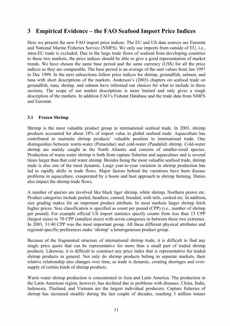
3 Empirical Evidence – the FAO Seafood Import Price Indices Here we present the new FAO import price indices. The EU and US data sources are Eurostat and National Marine Fisheries Service (NMFS). We only use imports from outside of EU, i.e., intra-EU trade is excluded. Due to the large trade flows of seafood from developing countries to these two markets, the price indices should be able to give a good representation of market trends. We have chosen the same base period and the same currency (US$) for all the price indices so they are comparable. The base period is an average of the unit values from Jan 1997 to Dec 1999. In the next subsections follow price indices for shrimp, groundfish, salmon, and tuna with short descriptions of the markets. Anderson’s (2003) chapters on seafood trade on groundfish, tuna, shrimp, and salmon have informed our choices for what to include in these sections. The scope of our market descriptions is more limited and only gives a rough description of the markets. In addition FAO’s Fishstat Database and the trade data from NMFS and Eurostat. 3.1 Frozen Shrimp Shrimp is the most valuable product group in international seafood trade. In 2003, shrimp products accounted for about 18% of import value in global seafood trade. Aquaculture has contributed to maintain shrimp products’ valuable position in international trade. One distinguishes between warm-water (Penaeidae) and cold-water (Pandalid) shrimp. Cold-water shrimp are mainly caught in the North Atlantic and consists of smaller-sized species. Production of warm water shrimp is both from capture fisheries and aquaculture and is several times larger than that cold water shrimp. Besides being the most valuable seafood trade, shrimp trade is also one of the most dynamic. Large year-to-year variation in shrimp production has led to rapidly shifts in trade flows. Major factors behind the variations have been disease problems in aquaculture, exasperated by a boom and bust approach to shrimp farming. Duties also impact the shrimp trade flows. A number of species are involved like black tiger shrimp, white shrimp, Northern prawn etc. Product categories include peeled, headless, canned, breaded, with tails, cooked etc. In addition, size grading makes for an important product attribute. In most markets larger shrimp fetch higher prices. Size classification is specified as count per pound (CPP) (i.e., number of shrimp per pound). For example official US import statistics specify counts from less than 15 CPP (largest sizes) to 70 CPP (smallest sizes) with seven categories in between these two extremes. In 2003, 31/40 CPP was the most important group. All these different physical attributes and regional-specific preferences make ‘shrimp’ a heterogeneous product group. Because of the fragmented structure of international shrimp trade, it is difficult to find any single price quote that can be representative for more than a small part of traded shrimp products. Likewise, it is difficult to construct any price index that is representative for traded shrimp products in general. Not only do shrimp products belong to separate markets, their relative relationship also changes over time, as trade is dynamic, creating shortages and over-supply of certain kinds of shrimp products. Warm water shrimp production is concentrated in Asia and Latin America. The production in the Latin American region, however, has declined due to problems with diseases. China, India, Indonesia, Thailand, and Vietnam are the largest individual producers. Capture fisheries of shrimp has increased steadily during the last couple of decades, reaching 3 million tonnes

12

in 2002. Shrimp aquaculture is of a new date and accounts for a growing share of global shrimp production. In 2002, 30.3% of global shrimp supply came from aquaculture. Aquaculture production is vulnerable to weather and disease outbreaks and sustainable production has proved a challenge. This has lead to large year-to-year variations in production.

0

100

200

300

400

500

600

1976

1978

1980

1982

1984

1986

1988

1990

1992

1994

1996

1998

2000

2002

1000

tonn

es

EUUSA

Figure 3.1. Apparent Shrimp Consumption in EU and USA (FAO Fishstat Database)

Figure 3.2 shows the import price indices for shrimp for EU and USA. It is difficult to construct two directly comparable price indices for shrimp between EU and USA because of different product groupings in their trade statistics. For frozen shrimp, EU distinguishes between Parapenaeus Longirostris, Penaeidae, Pandalid, and other shrimp (although, before 1997 the Eurostat only distinguish between Pandalid and other frozen shrimp) while the US distinguishes by size grading. The EU price index consists of all frozen shrimp and the US price index consists of five out of nine size grading – from 21 to 60 CPP.

0.00

0.20

0.40

0.60

0.80

1.00

1.20

1.40

1990

-7

1991

-4

1992

-1

1992

-10

1993

-7

1994

-4

1995

-1

1995

-10

1996

-7

1997

-4

1998

-1

1998

-10

1999

-7

2000

-4

2001

-1

2001

-10

2002

-7

2003

-4

2004

-1

SHRIMP EU frozen

SHRIMP US frozen

Figure 3.2. FAO Shrimp Price Indices for EU and USA (Base: 1997-1999 = 100)

13

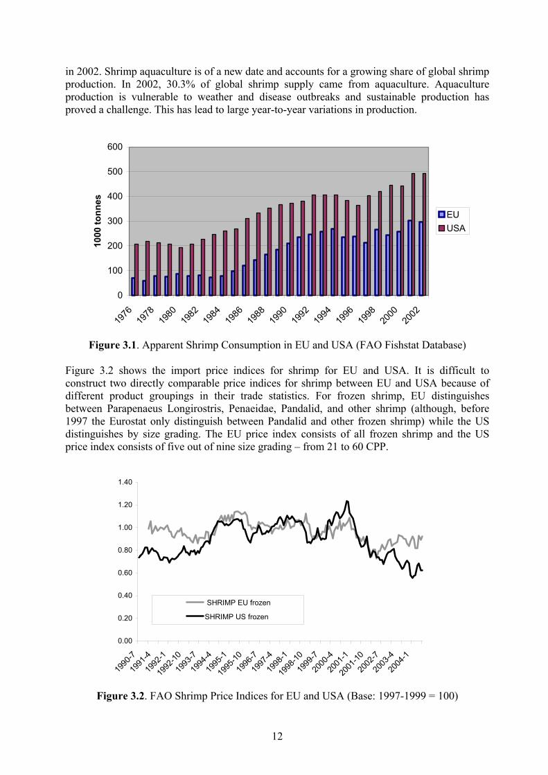
The EU shrimp prices were higher than in the USA until 1994, after which the shrimp prices have followed a similar trend in the EU and the US. From the end of 2000 both the EU and US prices fell markedly, but while the US prices have continued to fall, the EU prices started to rice again in the mid-2002. For the period as a whole, EU shrimp prices has trended slightly downward. Since shrimp supply to EU has increased substantially (as shown in figure 4), the modest reduction in prices must imply that the market has grown during this period. For the US the annual imports have fallen since the beginning of 1996. 3.2 Frozen Groundfish Groundfish is a composite of different species. In international trade the dominant species look similar, at least superficially, but are differently valued in the markets. These are cod, hake, haddock, pollock and saithe. Cod has one of the longest historical records in seafood trade, beginning from the 1500s with Basque fisheries outside of Newfoundland and onwards to current times where cod is still one of the most important traded groundfish, in particular Atlantic cod. Almost the entire groundfish production is from capture fisheries. Norway has experimented with cod aquaculture, hoping to make a commercial breakthrough with large-scale cod farming. This has yet to come. The top ten producers of cod, hake, haddock, pollock and saithe in 2002 were USA, Russian Federation, Norway, Island, Argentina, Faeroe Islands, Chile, Japan, New Zealand, and Denmark. They accounted for 84% of the global production of these groundfish species. Figure 3.3 shows that capture production of key groundfish species has shifted during the last decades due to overfishing. Atlantic cod, which entirely dominated trade until the 1970s, has been replaced by Alaska pollock as the leading species. Although Alaska pollock is still the dominating groundfish, the production has decreased during the last decade also due to overfishing.

0

2

4

6

8

10

12

14

16

1950

1955

1960

1965

1970

1975

1980

1985

1990

1995

2000

Mill

ion

tonn

es

Other groundfish

Haddock

Cape hakes

Pacif ic cod

Saithe(=Pollock)

Argentine hake

Atlantic cod

Blue w hiting(=Poutassou)

Alaska pollock(=Walleye poll)

Figure 3.3. Global Pollock, Cod, Hake, Haddock, and Saithe Catches (FAO Fishstat Database) Frozen groundfish consumption is much higher in the EU than in USA. Figure 3.4 shows a marked increase in the consumption of frozen groundfish in EU and a slight increase in USA.

14

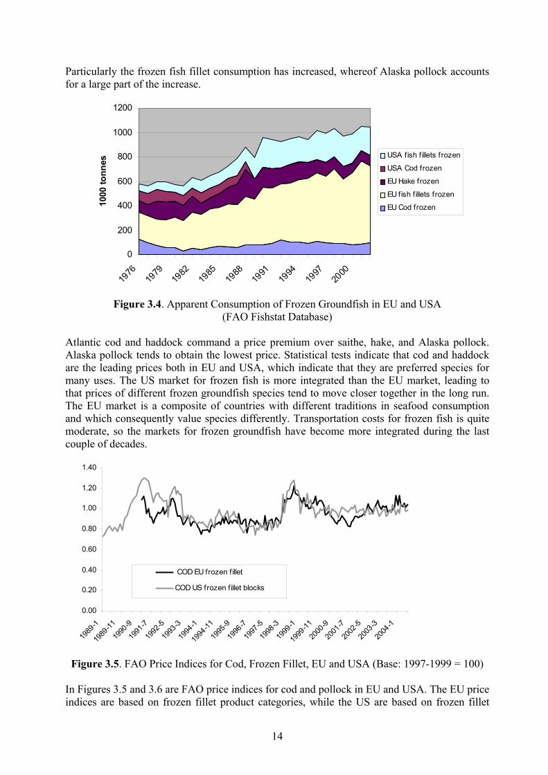
Particularly the frozen fish fillet consumption has increased, whereof Alaska pollock accounts for a large part of the increase.

0

200

400

600

800

1000

1200

1976

1979

1982

1985

1988

1991

1994

1997

2000

1000

tonn

es

USA fish f illets frozen

USA Cod frozen

EU Hake frozen

EU fish f illets frozen

EU Cod frozen

Figure 3.4. Apparent Consumption of Frozen Groundfish in EU and USA

(FAO Fishstat Database)

Atlantic cod and haddock command a price premium over saithe, hake, and Alaska pollock. Alaska pollock tends to obtain the lowest price. Statistical tests indicate that cod and haddock are the leading prices both in EU and USA, which indicate that they are preferred species for many uses. The US market for frozen fish is more integrated than the EU market, leading to that prices of different frozen groundfish species tend to move closer together in the long run. The EU market is a composite of countries with different traditions in seafood consumption and which consequently value species differently. Transportation costs for frozen fish is quite moderate, so the markets for frozen groundfish have become more integrated during the last couple of decades.

0.00

0.20

0.40

0.60

0.80

1.00

1.20

1.40

1989

-1

1989

-11

1990

-9

1991

-7

1992

-5

1993

-3

1994

-1

1994

-11

1995

-9

1996

-7

1997

-5

1998

-3

1999

-1

1999

-11

2000

-9

2001

-7

2002

-5

2003

-3

2004

-1

COD EU frozen f illet

COD US frozen f illet blocks

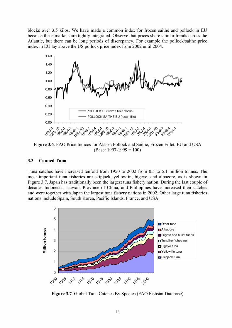
Figure 3.5. FAO Price Indices for Cod, Frozen Fillet, EU and USA (Base: 1997-1999 = 100)

In Figures 3.5 and 3.6 are FAO price indices for cod and pollock in EU and USA. The EU price indices are based on frozen fillet product categories, while the US are based on frozen fillet

15

blocks over 3.5 kilos. We have made a common index for frozen saithe and pollock in EU because these markets are tightly integrated. Observe that prices share similar trends across the Atlantic, but there can be long periods of discrepancy. For example the pollock/saithe price index in EU lay above the US pollock price index from 2002 until 2004.

0.00

0.20

0.40

0.60

0.80

1.00

1.20

1.40

1.60

1989

-1

1989

-10

1990

-7

1991

-4

1992

-1

1992

-10

1993

-7

1994

-4

1995

-1

1995

-10

1996

-7

1997

-4

1998

-1

1998

-10

1999

-7

2000

-4

2001

-1

2001

-10

2002

-7

2003

-4

2004

-1

POLLOCK US frozen fillet blocks

POLLOCK SAITHE EU frosen fillet

Figure 3.6. FAO Price Indices for Alaska Pollock and Saithe, Frozen Fillet, EU and USA

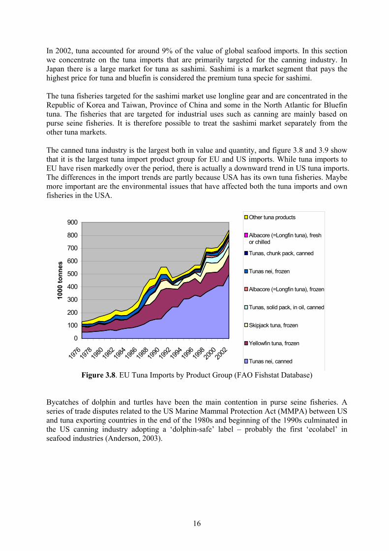
(Base: 1997-1999 = 100) 3.3 Canned Tuna Tuna catches have increased tenfold from 1950 to 2002 from 0.5 to 5.1 million tonnes. The most important tuna fisheries are skipjack, yellowfin, bigeye, and albacore, as is shown in Figure 3.7. Japan has traditionally been the largest tuna fishery nation. During the last couple of decades Indonesia, Taiwan, Province of China, and Philippines have increased their catches and were together with Japan the largest tuna fishery nations in 2002. Other large tuna fisheries nations include Spain, South Korea, Pacific Islands, France, and USA.

0

1

2

3

4

5

6

1950

1955

1960

1965

1970

1975

1980

1985

1990

1995

2000

Mill

ion

tonn

es

Other tuna

Albacore

Frigate and bullet tunas

Tunalike f ishes nei

Bigeye tuna

Yellow fin tuna

Skipjack tuna

Figure 3.7. Global Tuna Catches By Species (FAO Fishstat Database)

16

In 2002, tuna accounted for around 9% of the value of global seafood imports. In this section we concentrate on the tuna imports that are primarily targeted for the canning industry. In Japan there is a large market for tuna as sashimi. Sashimi is a market segment that pays the highest price for tuna and bluefin is considered the premium tuna specie for sashimi. The tuna fisheries targeted for the sashimi market use longline gear and are concentrated in the Republic of Korea and Taiwan, Province of China and some in the North Atlantic for Bluefin tuna. The fisheries that are targeted for industrial uses such as canning are mainly based on purse seine fisheries. It is therefore possible to treat the sashimi market separately from the other tuna markets. The canned tuna industry is the largest both in value and quantity, and figure 3.8 and 3.9 show that it is the largest tuna import product group for EU and US imports. While tuna imports to EU have risen markedly over the period, there is actually a downward trend in US tuna imports. The differences in the import trends are partly because USA has its own tuna fisheries. Maybe more important are the environmental issues that have affected both the tuna imports and own fisheries in the USA.

0

100

200

300

400

500

600

700

800

900

1976

1978

1980

1982

1984

1986

1988

1990

1992

1994

1996

1998

2000

2002

1000

tonn

es

Other tuna products

Albacore (=Longfin tuna), freshor chilled

Tunas, chunk pack, canned

Tunas nei, frozen

Albacore (=Longfin tuna), frozen

Tunas, solid pack, in oil, canned

Skipjack tuna, frozen

Yellowfin tuna, frozen

Tunas nei, canned

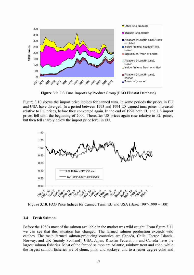
Figure 3.8. EU Tuna Imports by Product Group (FAO Fishstat Database) Bycatches of dolphin and turtles have been the main contention in purse seine fisheries. A series of trade disputes related to the US Marine Mammal Protection Act (MMPA) between US and tuna exporting countries in the end of the 1980s and beginning of the 1990s culminated in the US canning industry adopting a ‘dolphin-safe’ label – probably the first ‘ecolabel’ in seafood industries (Anderson, 2003).

17

0

50

100

150

200

250

300

350

400

1976

1978

1980

1982

1984

1986

1988

1990

1992

1994

1996

1998

2000

2002

1000

tonn

esOther tuna products

Skipjack tuna, frozen

Albacore (=Longfin tuna), freshor chilledYellow fin tuna, headsoff, etc,frozenBigeye tuna, fresh or chilled

Albacore (=Longfin tuna),frozenYellow fin tuna, fresh or chilled

Albacore (=Longfin tuna),cannedTunas nei, canned

Figure 3.9. US Tuna Imports by Product Group (FAO Fishstat Database)

Figure 3.10 shows the import price indices for canned tuna. In some periods the prices in EU and USA have diverged. In a period between 1993 and 1994 US canned tuna prices increased relative to EU prices, before they converged again. In the end of 1998 both EU and US import prices fell until the beginning of 2000. Thereafter US prices again rose relative to EU prices, but then fell sharply below the import price level in EU.

0.00

0.20

0.40

0.60

0.80

1.00

1.20

1.40

1989

-1

1989

-10

1990

-7

1991

-4

1992

-1

1992

-10

1993

-7

1994

-4

1995

-1

1995

-10

1996

-7

1997

-4

1998

-1

1998

-10

1999

-7

2000

-4

2001

-1

2001

-10

2002

-7

2003

-4

2004

-1

US TUNA NSPF OQ atc

EU TUNA NSPF conserved

Figure 3.10. FAO Price Indices for Canned Tuna, EU and USA (Base: 1997-1999 = 100)

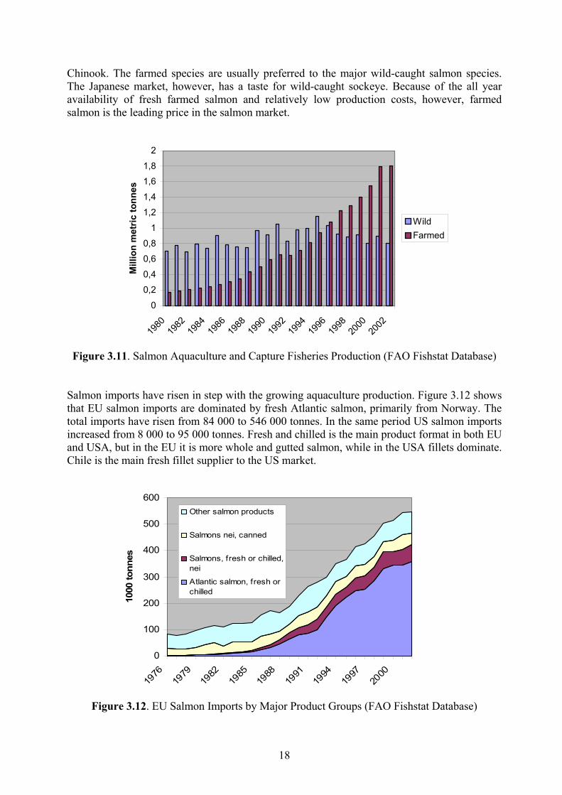
3.4 Fresh Salmon Before the 1980s most of the salmon available in the market was wild caught. From figure 3.11 we can see that this situation has changed. The farmed salmon production exceeds wild catches. The main farmed salmon-producing countries are Canada, Chile, Faeroe Islands, Norway, and UK (mainly Scotland). USA, Japan, Russian Federation, and Canada have the largest salmon fisheries. Most of the farmed salmon are Atlantic, rainbow trout and coho, while the largest salmon fisheries are of chum, pink, and sockeye, and to a lesser degree coho and

18

Chinook. The farmed species are usually preferred to the major wild-caught salmon species. The Japanese market, however, has a taste for wild-caught sockeye. Because of the all year availability of fresh farmed salmon and relatively low production costs, however, farmed salmon is the leading price in the salmon market.

0

0,2

0,4

0,6

0,8

1

1,2

1,4

1,6

1,8

2

1980

1982

1984

1986

1988

1990

1992

1994

1996

1998

2000

2002

Mill

ion

met

ric to

nnes

WildFarmed

Figure 3.11. Salmon Aquaculture and Capture Fisheries Production (FAO Fishstat Database)

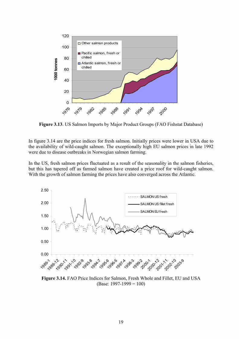
Salmon imports have risen in step with the growing aquaculture production. Figure 3.12 shows that EU salmon imports are dominated by fresh Atlantic salmon, primarily from Norway. The total imports have risen from 84 000 to 546 000 tonnes. In the same period US salmon imports increased from 8 000 to 95 000 tonnes. Fresh and chilled is the main product format in both EU and USA, but in the EU it is more whole and gutted salmon, while in the USA fillets dominate. Chile is the main fresh fillet supplier to the US market.

0

100

200

300

400

500

600

1976

1979

1982

1985

1988

1991

1994

1997

2000

1000

tonn

es

Other salmon products

Salmons nei, canned

Salmons, fresh or chilled,nei

Atlantic salmon, fresh orchilled

Figure 3.12. EU Salmon Imports by Major Product Groups (FAO Fishstat Database)

19

0

20

40

60

80

100

120

1976

1979

1982

1985

1988

1991

1994

1997

2000

1000

tonn

es

Other salmon products

Pacif ic salmon, fresh orchilled

Atlantic salmon, fresh orchilled

Figure 3.13. US Salmon Imports by Major Product Groups (FAO Fishstat Database)

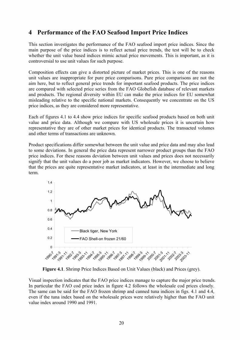
In figure 3.14 are the price indices for fresh salmon. Initially prices were lower in USA due to the availability of wild-caught salmon. The exceptionally high EU salmon prices in late 1992 were due to disease outbreaks in Norwegian salmon farming. In the US, fresh salmon prices fluctuated as a result of the seasonality in the salmon fisheries, but this has tapered off as farmed salmon have created a price roof for wild-caught salmon. With the growth of salmon farming the prices have also converged across the Atlantic.

0.00

0.50

1.00

1.50

2.00

2.50

1989

-1

1989

-12

1990

-11

1991

-10

1992

-9

1993

-8

1994

-7

1995

-6

1996

-5

1997

-4

1998

-3

1999

-2

2000

-1

2000

-12

2001

-11

2002

-10

2003

-9

SALMON US fresh

SALMON US fillet fresh

SALMON EU fresh

Figure 3.14. FAO Price Indices for Salmon, Fresh Whole and Fillet, EU and USA

(Base: 1997-1999 = 100)

20

4 Performance of the FAO Seafood Import Price Indices This section investigates the performance of the FAO seafood import price indices. Since the main purpose of the price indices is to reflect actual price trends, the test will be to check whether the unit value based indices mimic actual price movements. This is important, as it is controversial to use unit values for such purpose. Composition effects can give a distorted picture of market prices. This is one of the reasons unit values are inappropriate for pure price comparisons. Pure price comparisons are not the aim here, but to reflect general price trends for important seafood products. The price indices are compared with selected price series from the FAO Globefish database of relevant markets and products. The regional diversity within EU can make the price indices for EU somewhat misleading relative to the specific national markets. Consequently we concentrate on the US price indices, as they are considered more representative. Each of figures 4.1 to 4.4 show price indices for specific seafood products based on both unit value and price data. Although we compare with US wholesale prices it is uncertain how representative they are of other market prices for identical products. The transacted volumes and other terms of transactions are unknown. Product specifications differ somewhat between the unit value and price data and may also lead to some deviations. In general the price data represent narrower product groups than the FAO price indices. For these reasons deviation between unit values and prices does not necessarily signify that the unit values do a poor job as market indicators. However, we choose to believe that the prices are quite representative market indicators, at least in the intermediate and long term.

0

0.2

0.4

0.6

0.8

1

1.2

1.4

1990

-7

1991

-3

1991

-11

1992

-7

1993

-3

1993

-11

1994

-7

1995

-3

1995

-11

1996

-7

1997

-3

1997

-11

1998

-7

1999

-3

1999

-11

2000

-7

2001

-3

2001

-11

2002

-7

2003

-3

2003

-11

Black tiger, New York

FAO Shell-on frozen 21/60

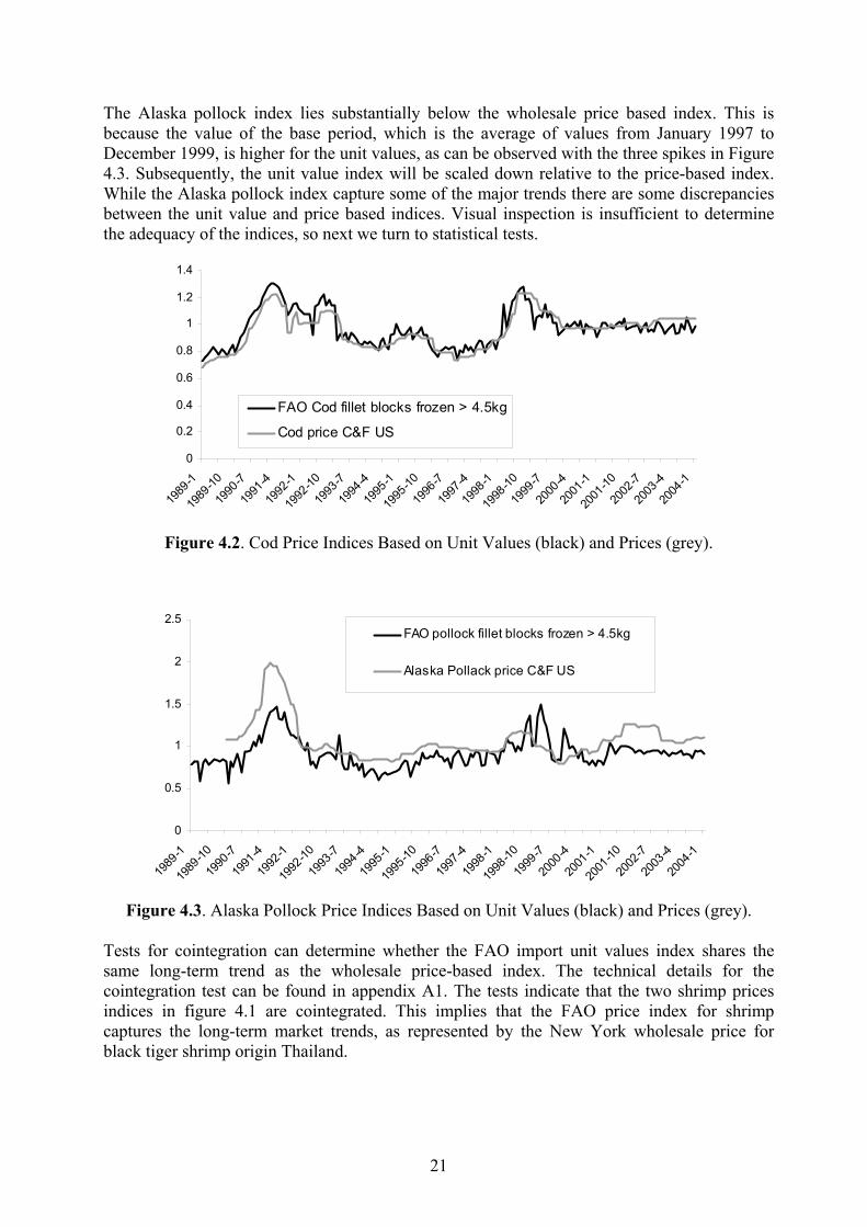
Figure 4.1. Shrimp Price Indices Based on Unit Values (black) and Prices (grey).

Visual inspection indicates that the FAO price indices manage to capture the major price trends. In particular the FAO cod price index in figure 4.2 follows the wholesale cod prices closely. The same can be said for the FAO frozen shrimp and canned tuna indices in figs. 4.1 and 4.4, even if the tuna index based on the wholesale prices were relatively higher than the FAO unit value index around 1990 and 1991.

21

The Alaska pollock index lies substantially below the wholesale price based index. This is because the value of the base period, which is the average of values from January 1997 to December 1999, is higher for the unit values, as can be observed with the three spikes in Figure 4.3. Subsequently, the unit value index will be scaled down relative to the price-based index. While the Alaska pollock index capture some of the major trends there are some discrepancies between the unit value and price based indices. Visual inspection is insufficient to determine the adequacy of the indices, so next we turn to statistical tests.

0

0.2

0.4

0.6

0.8

1

1.2

1.4

1989

-1

1989

-10

1990

-7

1991

-4

1992

-1

1992

-10

1993

-7

1994

-4

1995

-1

1995

-10

1996

-7

1997

-4

1998

-1

1998

-10

1999

-7

2000

-4

2001

-1

2001

-10

2002

-7

2003

-4

2004

-1

FAO Cod fillet blocks frozen > 4.5kg

Cod price C&F US

Figure 4.2. Cod Price Indices Based on Unit Values (black) and Prices (grey).

0

0.5

1

1.5

2

2.5

1989

-1

1989

-10

1990

-7

1991

-4

1992

-1

1992

-10

1993

-7

1994

-4

1995

-1

1995

-10

1996

-7

1997

-4

1998

-1

1998

-10

1999

-7

2000

-4

2001

-1

2001

-10

2002

-7

2003

-4

2004

-1

FAO pollock fillet blocks frozen > 4.5kg

Alaska Pollack price C&F US

Figure 4.3. Alaska Pollock Price Indices Based on Unit Values (black) and Prices (grey).

Tests for cointegration can determine whether the FAO import unit values index shares the same long-term trend as the wholesale price-based index. The technical details for the cointegration test can be found in appendix A1. The tests indicate that the two shrimp prices indices in figure 4.1 are cointegrated. This implies that the FAO price index for shrimp captures the long-term market trends, as represented by the New York wholesale price for black tiger shrimp origin Thailand.

22

0

0.2

0.4

0.6

0.8

1

1.2

1.4

1989

-1

1989

-10

1990

-7

1991

-4

1992

-1

1992

-10

1993

-7

1994

-4

1995

-1

1995

-10

1996

-7

1997

-4

1998

-1

1998

-10

1999

-7

2000

-4

2001

-1

2001

-10

2002

-7

2003

-4

2004

-1

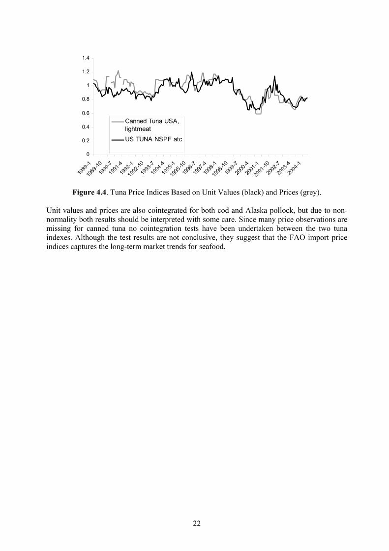
Canned Tuna USA,lightmeatUS TUNA NSPF atc

Figure 4.4. Tuna Price Indices Based on Unit Values (black) and Prices (grey).

Unit values and prices are also cointegrated for both cod and Alaska pollock, but due to non-normality both results should be interpreted with some care. Since many price observations are missing for canned tuna no cointegration tests have been undertaken between the two tuna indexes. Although the test results are not conclusive, they suggest that the FAO import price indices captures the long-term market trends for seafood.

23

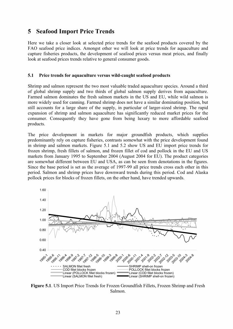
5 Seafood Import Price Trends Here we take a closer look at selected price trends for the seafood products covered by the FAO seafood price indices. Amongst other we will look at price trends for aquaculture and capture fisheries products, the development of seafood prices versus meat prices, and finally look at seafood prices trends relative to general consumer goods. 5.1 Price trends for aquaculture versus wild-caught seafood products Shrimp and salmon represent the two most valuable traded aquaculture species. Around a third of global shrimp supply and two thirds of global salmon supply derives from aquaculture. Farmed salmon dominates the fresh salmon markets in the US and EU, while wild salmon is more widely used for canning. Farmed shrimp does not have a similar dominating position, but still accounts for a large share of the supply, in particular of larger-sized shrimp. The rapid expansion of shrimp and salmon aquaculture has significantly reduced market prices for the consumer. Consequently they have gone from being luxury to more affordable seafood products. The price development in markets for major groundfish products, which supplies predominantly rely on capture fisheries, contrasts somewhat with the price development found in shrimp and salmon markets. Figure 5.1 and 5.2 show US and EU import price trends for frozen shrimp, fresh fillets of salmon, and frozen fillet of cod and pollock in the EU and US markets from January 1995 to September 2004 (August 2004 for EU). The product categories are somewhat different between EU and USA, as can be seen from denotations in the figures. Since the base period is set as the average of 1997-99 all price trends cross each other in this period. Salmon and shrimp prices have downward trends during this period. Cod and Alaska pollock prices for blocks of frozen fillets, on the other hand, have trended upwards.

0.40

0.60

0.80

1.00

1.20

1.40

1.60

1995

-1

1995

-6

1995

-11

1996

-4

1996

-9

1997

-2

1997

-7

1997

-12

1998

-5

1998

-10

1999

-3

1999

-8

2000

-1

2000

-6

2000

-11

2001

-4

2001

-9

2002

-2

2002

-7

2002

-12

2003

-5

2003

-10

2004

-3

2004

-8

SALMON fillet fresh SHRIMP shell-on frozenCOD fillet blocks frozen POLLOCK fillet blocks frozenLinear (POLLOCK fillet blocks frozen) Linear (COD fillet blocks frozen)Linear (SALMON fillet fresh) Linear (SHRIMP shell-on frozen)

Figure 5.1. US Import Price Trends for Frozen Groundfish Fillets, Frozen Shrimp and Fresh

Salmon.

24

0.4

0.6

0.8

1

1.2

1.4

1.6

1995

-01

1995

-07

1996

-01

1996

-07

1997

-01

1997

-07

1998

-01

1998

-07

1999

-01

1999

-07

2000

-01

2000

-07

2001

-01

2001

-07

2002

-01

2002

-07

2003

-01

2003

-07

2004

-01

2004

-07

SHRIMP frozen POLLOCK SAITHE frosen f illet COD frozen fillet SALMON freshLinear ( SALMON fresh) Linear ( SHRIMP frozen)Linear ( POLLOCK SAITHE frosen f illet) Linear ( COD frozen fillet)

Figure 5.2. EU Import Price Trends for Frozen Groundfish Fillets, Frozen Shrimp and Fresh

Salmon. Frozen cod imports peaked in the early 1990s and have decreased since, dropping from the position as one of the most valuable seafood imports in the US. Lower catches of cod, in particular Atlantic cod, have negatively impacted the import quantities. Increasing Alaska pollock imports may have compensated somewhat the downfall in cod imports, as they are substitutes in some uses, albeit not perfect ones, since Alaska pollock is considered inferior to Atlantic cod. The import volumes of frozen fillets of Alaska pollock have exceeded that of cod since the mid-nineties as shown in figure 5.3. A similar development to that in USA is found in the imports of cod and Alaska pollock to the EU.

0

20

40

60

80

100

120

140

160

180

1990 1991 1992 1993 1994 1995 1996 1997 1998 1999 2000 2001 2002 2003

1000

tons

ATLANTIC COD ALASKA POLLOCK

Figure 5.3. US Imports of Atlantic Cod and Alaska Pollock Frozen Fillets (NMFS)

25

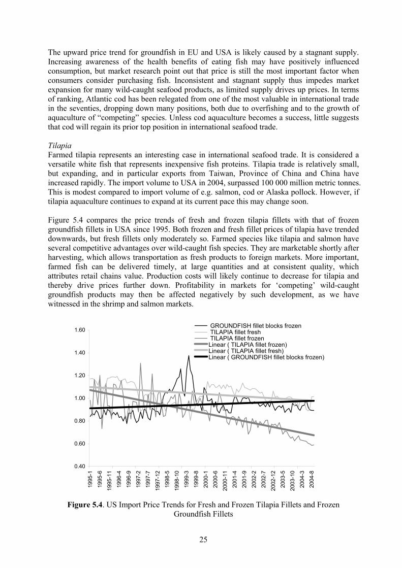
The upward price trend for groundfish in EU and USA is likely caused by a stagnant supply. Increasing awareness of the health benefits of eating fish may have positively influenced consumption, but market research point out that price is still the most important factor when consumers consider purchasing fish. Inconsistent and stagnant supply thus impedes market expansion for many wild-caught seafood products, as limited supply drives up prices. In terms of ranking, Atlantic cod has been relegated from one of the most valuable in international trade in the seventies, dropping down many positions, both due to overfishing and to the growth of aquaculture of “competing” species. Unless cod aquaculture becomes a success, little suggests that cod will regain its prior top position in international seafood trade. Tilapia Farmed tilapia represents an interesting case in international seafood trade. It is considered a versatile white fish that represents inexpensive fish proteins. Tilapia trade is relatively small, but expanding, and in particular exports from Taiwan, Province of China and China have increased rapidly. The import volume to USA in 2004, surpassed 100 000 million metric tonnes. This is modest compared to import volume of e.g. salmon, cod or Alaska pollock. However, if tilapia aquaculture continues to expand at its current pace this may change soon. Figure 5.4 compares the price trends of fresh and frozen tilapia fillets with that of frozen groundfish fillets in USA since 1995. Both frozen and fresh fillet prices of tilapia have trended downwards, but fresh fillets only moderately so. Farmed species like tilapia and salmon have several competitive advantages over wild-caught fish species. They are marketable shortly after harvesting, which allows transportation as fresh products to foreign markets. More important, farmed fish can be delivered timely, at large quantities and at consistent quality, which attributes retail chains value. Production costs will likely continue to decrease for tilapia and thereby drive prices further down. Profitability in markets for ‘competing’ wild-caught groundfish products may then be affected negatively by such development, as we have witnessed in the shrimp and salmon markets.

0.40

0.60

0.80

1.00

1.20

1.40

1.60

1995

-1

1995

-6

1995

-11

1996

-4

1996

-9

1997

-2

1997

-7

1997

-12

1998

-5

1998

-10

1999

-3

1999

-8

2000

-1

2000

-6

2000

-11

2001

-4

2001

-9

2002

-2

2002

-7

2002

-12

2003

-5

2003

-10

2004

-3

2004

-8

GROUNDFISH fillet blocks frozen TILAPIA fillet fresh TILAPIA fillet frozenLinear ( TILAPIA fillet frozen)Linear ( TILAPIA fillet fresh)Linear ( GROUNDFISH fillet blocks frozen)

Figure 5.4. US Import Price Trends for Fresh and Frozen Tilapia Fillets and Frozen

Groundfish Fillets

26

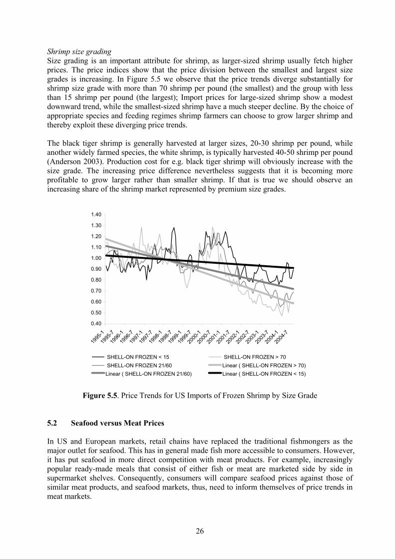
Shrimp size grading Size grading is an important attribute for shrimp, as larger-sized shrimp usually fetch higher prices. The price indices show that the price division between the smallest and largest size grades is increasing. In Figure 5.5 we observe that the price trends diverge substantially for shrimp size grade with more than 70 shrimp per pound (the smallest) and the group with less than 15 shrimp per pound (the largest); Import prices for large-sized shrimp show a modest downward trend, while the smallest-sized shrimp have a much steeper decline. By the choice of appropriate species and feeding regimes shrimp farmers can choose to grow larger shrimp and thereby exploit these diverging price trends. The black tiger shrimp is generally harvested at larger sizes, 20-30 shrimp per pound, while another widely farmed species, the white shrimp, is typically harvested 40-50 shrimp per pound (Anderson 2003). Production cost for e.g. black tiger shrimp will obviously increase with the size grade. The increasing price difference nevertheless suggests that it is becoming more profitable to grow larger rather than smaller shrimp. If that is true we should observe an increasing share of the shrimp market represented by premium size grades.

0.40

0.50

0.60

0.70

0.80

0.90

1.00

1.10

1.20

1.30

1.40

1995

-1

1995

-7

1996

-1

1996

-7

1997

-1

1997

-7

1998

-1

1998

-7

1999

-1

1999

-7

2000

-1

2000

-7

2001

-1

2001

-7

2002

-1

2002

-7

2003

-1

2003

-7

2004

-1

2004

-7

SHELL-ON FROZEN < 15 SHELL-ON FROZEN > 70 SHELL-ON FROZEN 21/60 Linear ( SHELL-ON FROZEN > 70)Linear ( SHELL-ON FROZEN 21/60) Linear ( SHELL-ON FROZEN < 15)

Figure 5.5. Price Trends for US Imports of Frozen Shrimp by Size Grade

5.2 Seafood versus Meat Prices In US and European markets, retail chains have replaced the traditional fishmongers as the major outlet for seafood. This has in general made fish more accessible to consumers. However, it has put seafood in more direct competition with meat products. For example, increasingly popular ready-made meals that consist of either fish or meat are marketed side by side in supermarket shelves. Consequently, consumers will compare seafood prices against those of similar meat products, and seafood markets, thus, need to inform themselves of price trends in meat markets.

27

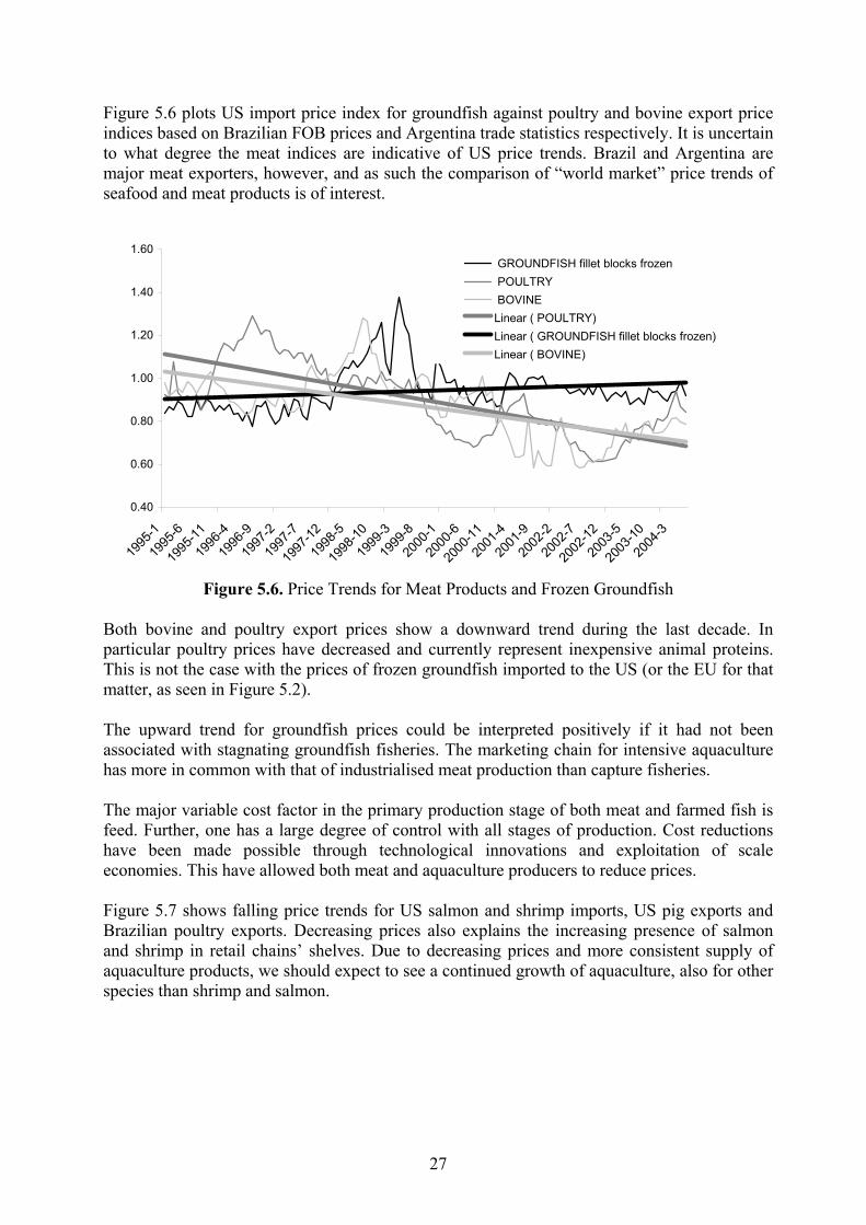
Figure 5.6 plots US import price index for groundfish against poultry and bovine export price indices based on Brazilian FOB prices and Argentina trade statistics respectively. It is uncertain to what degree the meat indices are indicative of US price trends. Brazil and Argentina are major meat exporters, however, and as such the comparison of “world market” price trends of seafood and meat products is of interest.

0.40

0.60

0.80

1.00

1.20

1.40

1.60

1995

-1

1995

-6

1995

-11

1996

-4

1996

-9

1997

-2

1997

-7

1997

-12

1998

-5

1998

-10

1999

-3

1999

-8

2000

-1

2000

-6

2000

-11

2001

-4

2001

-9

2002

-2

2002

-7

2002

-12

2003

-5

2003

-10

2004

-3

GROUNDFISH fillet blocks frozen POULTRY BOVINELinear ( POULTRY)Linear ( GROUNDFISH fillet blocks frozen)Linear ( BOVINE)

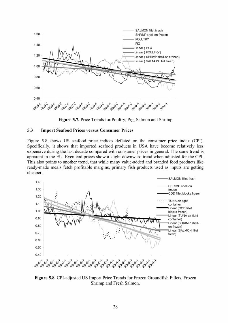
Figure 5.6. Price Trends for Meat Products and Frozen Groundfish Both bovine and poultry export prices show a downward trend during the last decade. In particular poultry prices have decreased and currently represent inexpensive animal proteins. This is not the case with the prices of frozen groundfish imported to the US (or the EU for that matter, as seen in Figure 5.2). The upward trend for groundfish prices could be interpreted positively if it had not been associated with stagnating groundfish fisheries. The marketing chain for intensive aquaculture has more in common with that of industrialised meat production than capture fisheries. The major variable cost factor in the primary production stage of both meat and farmed fish is feed. Further, one has a large degree of control with all stages of production. Cost reductions have been made possible through technological innovations and exploitation of scale economies. This have allowed both meat and aquaculture producers to reduce prices. Figure 5.7 shows falling price trends for US salmon and shrimp imports, US pig exports and Brazilian poultry exports. Decreasing prices also explains the increasing presence of salmon and shrimp in retail chains’ shelves. Due to decreasing prices and more consistent supply of aquaculture products, we should expect to see a continued growth of aquaculture, also for other species than shrimp and salmon.

28

0.40

0.60

0.80

1.00

1.20

1.40

1.60

1995

-1

1995

-7

1996

-1

1996

-7

1997

-1

1997

-7

1998

-1

1998

-7

1999

-1

1999

-7

2000

-1

2000

-7

2001

-1

2001

-7

2002

-1

2002

-7

2003

-1

2003

-7

2004

-1

SALMON fillet fresh SHRIMP shell-on frozen POULTRY PIGLinear ( PIG)Linear ( POULTRY)Linear ( SHRIMP shell-on frozen)Linear ( SALMON fillet fresh)

Figure 5.7. Price Trends for Poultry, Pig, Salmon and Shrimp

5.3 Import Seafood Prices versus Consumer Prices Figure 5.8 shows US seafood price indices deflated on the consumer price index (CPI). Specifically, it shows that imported seafood products in USA have become relatively less expensive during the last decade compared with consumer prices in general. The same trend is apparent in the EU. Even cod prices show a slight downward trend when adjusted for the CPI. This also points to another trend, that while many value-added and branded food products like ready-made meals fetch profitable margins, primary fish products used as inputs are getting cheaper.

0.40

0.50

0.60

0.70

0.80

0.90

1.00

1.10

1.20

1.30

1.40

1995

-1

1995

-7

1996

-1

1996

-7

1997

-1

1997

-7

1998

-1

1998

-7

1999

-1

1999

-7

2000

-1

2000

-7

2001

-1

2001

-7

2002

-1

2002

-7

2003

-1

2003

-7

2004

-1

2004

-7

SALMON fillet fresh

SHRIMP shell-onfrozenCOD fillet blocks frozen

TUNA air tightcontainerLinear (COD filletblocks frozen)Linear (TUNA air tightcontainer)Linear (SHRIMP shell-on frozen)Linear (SALMON filletfresh)

Figure 5.8. CPI-adjusted US Import Price Trends for Frozen Groundfish Fillets, Frozen Shrimp and Fresh Salmon.

29

Higher profit margins in agrifood and seafood industries are increasingly related to value-added processing. The challenge for fishermen and fish farmers who are not involved in later processing stages, thus, is to remain competitive by keeping costs low and providing high-quality products. Requirements for more efficient seafood distribution, however, is seeing more and more primary producers getting integrated in seafood supply chains, e.g. large seafood companies that produce, process, and distribute final consumer products. This trend will likely continue, as such arrangements better satisfy retail chains requirements.

30

Reference:

Allen, R. G. D. 1975. Index Numbers in Theory and Practice. Macmillan. London.

Anderson, James L. 2003. The International Seafood Trade. Woodhead Publishing Ltd. Cambridge, England.

Asche, F., H. Bremnes, and C. R. Wessells. 1999. “Product Aggregation, Market Integration and Relationships Between Prices: An Application to World Salmon Markets.” American Journal of Agricultural Economics, 81, 568-581.

Asche, Frank, Guttormsen, Atle, og Sigbjørn Tveterås. 2001. ”Aggregation over different qualities: Are there generic commodities?” Economics Bulletin, 3(13).

Cournot, A. A. 1971. Researches into the Mathematical Principles of the Theory of Wealth, New York. A. M. Kelly.

Diewert, W. Erwin 1987, 'Index Numbers' in Eatwell, J., M. Milgate, and P. Newman, eds The New Palgrave: A Dictionary of Economics, London: The Macmillan Press, 1987, pp. 767-80.

Doglia, Marco. 1999. Seafood Price Indices. Fishery Industries Division, Special Series no.6. Food and Agriculture Organization of the United Nations, Rome.

FAO. 2002. Construction of a New FAO Export Price on Rice. Unpublished document. Food and Agriculture Organization of the United Nations, Rome.

Hicks, J. R. Value and capital. Oxford: Oxford University Press 1936.

Kiel, Frank. 1993. FAO Import Price Indices for Major International Fishery Products. FAO Fisheries Circular No. 860. Food and Agriculture Organization of the United Nations, Rome.

Leontief, W. 1936. Composite Commodities and the Problem of Index Numbers. Econometrica, 4:39-59.

Lewbel, A. 1996. “Aggregation without Separability: A Generalized Composite Commodity Theorem.” American Economic Review, 86, 524-561.

MacKinnon, J. 1991. Critical values for co-integration tests, in R.F Engle and C.W.J. Granger (eds.). Long-Run Economic Relationships. Oxford University Press. Oxford.

Stigler, G. J. 1969. The Theory of Price. Macmillan Company. London.

United Nations. 1977. Guidelines on principles of a system of price and quantity statistics. Statistical papers, series M, no. 59, UN. New York.

Von der Lippe, P. 1985. Wirtschaftstatistik. Fisher, Stutgart, New York. Pp. 248-297.

Von der Lippe, P. 2002. TES Course on Price Statistics and Price Index Theory. < http://www.vwl.uni-essen.de/dt/stat/dokumente/tes/preb11.pdf >

31

6 Appendices 6.1 Johansen Multivariate Cointegration

We will investigate the relationships between prices using the Johansen test (1991). The Johansen test is based on a VAR system. A vector, xt, containing the N variables to be tested for cointegration, is assumed to be generated by an unrestricted kth order vector autoregression in the levels of the variables; x x xt t k t k t tD e= + + + + +− −Π Π Φ1 1 ... µ (3) where each Πi is a (N × N) matrix of parameters, µ a constant term and εt∼niid(0,Ω). The VAR system of equations in (4) written in error correction form (ECM) is;

∆ Γ ∆ Πx x xt ii

k

t i K t k te= + + +=

−

− −∑1

1

µ (4)

with ,...1 ii I Π++Π+−=Γ 1,...,1 −= ki and Π Π ΠK kI= − + + +1 ... . Hence, ΠK is the long-run 'level solution' to (3). If xt is a vector of I(1) variables, the left-hand side and the first (k-1) elements of (4) are I(0), and the last element of (4) is a linear combination of I(1) variables. Given the assumption on the error term, this last element must also be I(0); Π K t kx − ∼I(0). Hence, either xt contains a number of cointegration vectors, or ΠK must be a matrix of zeros. The rank of ΠK, r, determines how many linear combinations of xt are stationary. If r = N, the variables in levels are stationary; if r = 0 so that ΠK =0, none of the linear combinations are stationary. When 0 < r < N, there exist r cointegration vectors - or r stationary linear combinations of xt. In this case one can factorise ΠK; − = ′ΠK αβ , where both α and β are (N × r) matrices, and β contains the cointegration vectors (the error correcting mechanism in the system) and α the factor loadings. Two asymptotically equivalent tests exist in this framework, the trace test and the maximum eigenvalue test. In our empirical applications, the xt vector contains three data series, the two prices and the exchange rate. We will expect to find one cointegration vector if there is a relationship between the two markets. The Johansen procedure allows hypothesis testing on the coefficients α and β , using likelihood ratio tests (Johansen and Juselius, 1990). Provided that the data series are cointegrated and we find one cointegration vector, the rank of βα ′=Π is equal to 1 and α and β are (3 × 1) vectors. A test of full exchange rate pass-through is then a test of whether β'=(1,-b,b)' and is distributed as χ2(1), while a test for the ‘law of one price’ is a test of whether β'=(1,-1,-1)' and is distributed as χ2(2). The factor loadings α are of interest as they contain information about exogeneity (Johansen and Juselius, 1990), and therefore also about leading prices or central markets. If a row in α contains only zeros (or in our case one element since α is a column vector), the price in question will be weakly exogenous, or decided outside of the system. Hence, if the factor loading parameter in the equation for the exchange rate is zero, the data indicate that the exchanges rate is decided outside of the system. Furthermore, if the factor loading parameter associated with one of the prices is zero, this price will be determined outside of the system, and will therefore be the leading price. With one cointegration vector, at least one factor loading parameter must be different from zero (Johansen and Juselius, 1990). Also note that only in the case when just one factor loading parameter is different from zero will there be no simultaneity problems if a system is represented with a single equation specification (normalised on the correct variable). On this background we may now proceed with two case studies with application of the market integration framework.

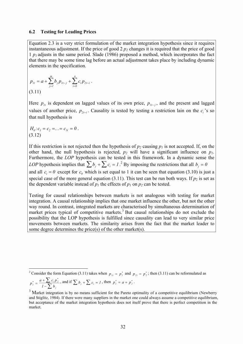
32

6.2 Testing for Leading Prices Equation 2.3 is a very strict formulation of the market integration hypothesis since it requires instantaneous adjustment. If the price of good 2 p2 changes it is required that the price of good 1 p1 adjusts in the same period. Slade (1986) proposed a method, which incorporates the fact that there may be some time lag before an actual adjustment takes place by including dynamic elements in the specification.

p a b p c pt jj

m

t j i t ii

n

11

1 20

= + +=

− −=

∑ ∑ .

(3.11) Here p t1 is dependent on lagged values of its own price, p t j1 − , and the present and lagged values of another price, p t i2 − . Causality is tested by testing a restriction lain on the ci ’s so that null hypothesis is H c c cN0 1 2 0: ...= = = = . (3.12) If this restriction is not rejected then the hypothesis of p2 causing p1 is not accepted. If, on the other hand, the null hypothesis is rejected, p2 will have a significant influence on p1. Furthermore, the LOP hypothesis can be tested in this framework. In a dynamic sense the LOP hypothesis implies that b cj i+ =∑∑ 1 .2 By imposing the restrictions that all bj = 0 and all ci = 0 except for c0 which is set equal to 1 it can be seen that equation (3.10) is just a special case of the more general equation (3.11). This test can be run both ways. If p2 is set as the dependent variable instead of p1 the effects of p1 on p2 can be tested. Testing for causal relationships between markets is not analogous with testing for market integration. A causal relationship implies that one market influence the other, but not the other way round. In contrast, integrated markets are characterised by simultaneous determination of market prices typical of competitive markets.3 But causal relationships do not exclude the possibility that the LOP hypothesis is fulfilled since causality can lead to very similar price movements between markets. The similarity arises from the fact that the market leader to some degree determines the price(s) of the other market(s).

2 Consider the form Equation (3.11) takes when p pt1 1= * and p pt2 2= * ; then (3.11) can be reformulated as

pa c p

bi

j1

2

1*

*

=+

−∑∑

, and if b cj i+ =∑∑ 1 , then p a p1 2* *= + .

3 Market integration is by no means sufficient for the Pareto optimality of a competitive equilibrium (Newberry and Stiglitz, 1984). If there were many suppliers in the market one could always assume a competitive equilibrium, but acceptance of the market integration hypothesis does not itself prove that there is perfect competition in the market.

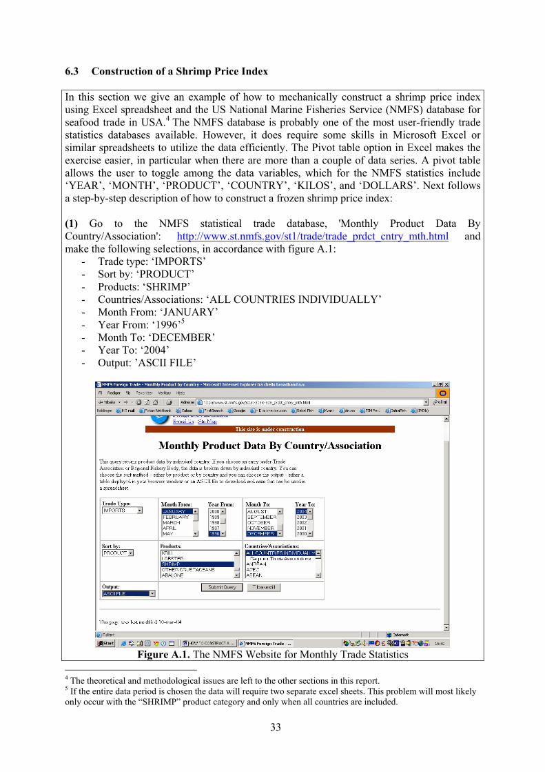
33

6.3 Construction of a Shrimp Price Index In this section we give an example of how to mechanically construct a shrimp price index using Excel spreadsheet and the US National Marine Fisheries Service (NMFS) database for seafood trade in USA.4 The NMFS database is probably one of the most user-friendly trade statistics databases available. However, it does require some skills in Microsoft Excel or similar spreadsheets to utilize the data efficiently. The Pivot table option in Excel makes the exercise easier, in particular when there are more than a couple of data series. A pivot table allows the user to toggle among the data variables, which for the NMFS statistics include ‘YEAR’, ‘MONTH’, ‘PRODUCT’, ‘COUNTRY’, ‘KILOS’, and ‘DOLLARS’. Next follows a step-by-step description of how to construct a frozen shrimp price index: (1) Go to the NMFS statistical trade database, 'Monthly Product Data By Country/Association': http://www.st.nmfs.gov/st1/trade/trade_prdct_cntry_mth.html and make the following selections, in accordance with figure A.1:

- Trade type: ‘IMPORTS’ - Sort by: ‘PRODUCT’ - Products: ‘SHRIMP’ - Countries/Associations: ‘ALL COUNTRIES INDIVIDUALLY’ - Month From: ‘JANUARY’ - Year From: ‘1996’5 - Month To: ‘DECEMBER’ - Year To: ‘2004’ - Output: ’ASCII FILE’

Figure A.1. The NMFS Website for Monthly Trade Statistics

4 The theoretical and methodological issues are left to the other sections in this report. 5 If the entire data period is chosen the data will require two separate excel sheets. This problem will most likely only occur with the “SHRIMP” product category and only when all countries are included.

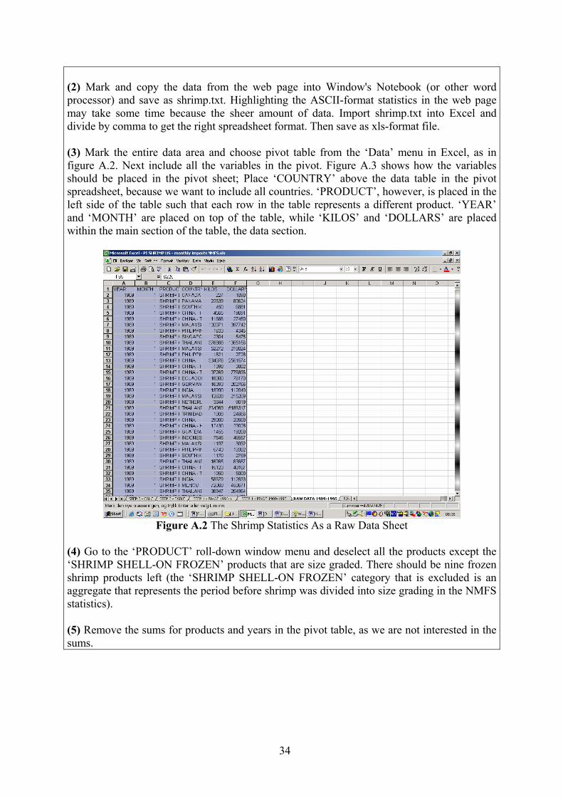
34

(2) Mark and copy the data from the web page into Window's Notebook (or other word processor) and save as shrimp.txt. Highlighting the ASCII-format statistics in the web page may take some time because the sheer amount of data. Import shrimp.txt into Excel and divide by comma to get the right spreadsheet format. Then save as xls-format file. (3) Mark the entire data area and choose pivot table from the ‘Data’ menu in Excel, as in figure A.2. Next include all the variables in the pivot. Figure A.3 shows how the variables should be placed in the pivot sheet; Place ‘COUNTRY’ above the data table in the pivot spreadsheet, because we want to include all countries. ‘PRODUCT’, however, is placed in the left side of the table such that each row in the table represents a different product. ‘YEAR’ and ‘MONTH’ are placed on top of the table, while ‘KILOS’ and ‘DOLLARS’ are placed within the main section of the table, the data section.

Figure A.2 The Shrimp Statistics As a Raw Data Sheet

(4) Go to the ‘PRODUCT’ roll-down window menu and deselect all the products except the ‘SHRIMP SHELL-ON FROZEN’ products that are size graded. There should be nine frozen shrimp products left (the ‘SHRIMP SHELL-ON FROZEN’ category that is excluded is an aggregate that represents the period before shrimp was divided into size grading in the NMFS statistics). (5) Remove the sums for products and years in the pivot table, as we are not interested in the sums.

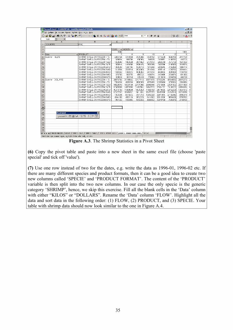
35

Figure A.3. The Shrimp Statistics in a Pivot Sheet

(6) Copy the pivot table and paste into a new sheet in the same excel file (choose 'paste special' and tick off 'value'). (7) Use one row instead of two for the dates, e.g. write the data as 1996-01, 1996-02 etc. If there are many different species and product formats, then it can be a good idea to create two new columns called ‘SPECIE’ and ‘PRODUCT FORMAT’. The content of the ‘PRODUCT’ variable is then split into the two new columns. In our case the only specie is the generic category ‘SHRIMP’, hence, we skip this exercise. Fill all the blank cells in the ‘Data’ column with either “KILOS” or “DOLLARS”. Rename the ‘Data’ column ‘FLOW’. Highlight all the data and sort data in the following order: (1) FLOW, (2) PRODUCT, and (3) SPECIE. Your table with shrimp data should now look similar to the one in Figure A.4.

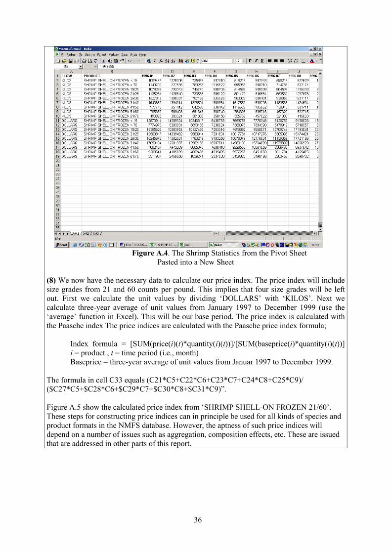
36

Figure A.4. The Shrimp Statistics from the Pivot Sheet

Pasted into a New Sheet (8) We now have the necessary data to calculate our price index. The price index will include size grades from 21 and 60 counts per pound. This implies that four size grades will be left out. First we calculate the unit values by dividing ‘DOLLARS’ with ‘KILOS’. Next we calculate three-year average of unit values from January 1997 to December 1999 (use the ‘average’ function in Excel). This will be our base period. The price index is calculated with the Paasche index The price indices are calculated with the Paasche price index formula; Index formula = [SUM(price(i)(t)*quantity(i)(t))]/[SUM(baseprice(i)*quantity(i)(t))] i = product , t = time period (i.e., month) Baseprice = three-year average of unit values from Januar 1997 to December 1999. The formula in cell C33 equals (C21*C5+C22*C6+C23*C7+C24*C8+C25*C9)/ ($C27*C5+$C28*C6+$C29*C7+$C30*C8+$C31*C9)”. Figure A.5 show the calculated price index from ‘SHRIMP SHELL-ON FROZEN 21/60’. These steps for constructing price indices can in principle be used for all kinds of species and product formats in the NMFS database. However, the aptness of such price indices will depend on a number of issues such as aggregation, composition effects, etc. These are issued that are addressed in other parts of this report.

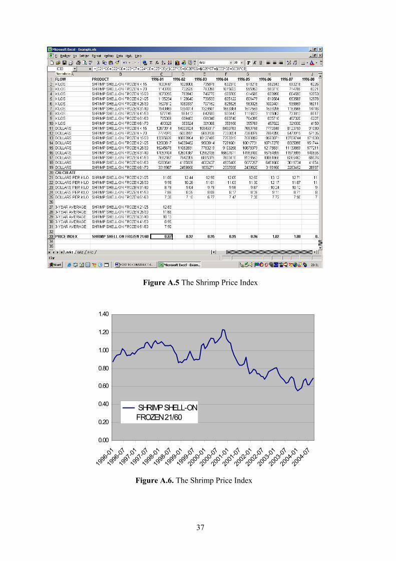
37

Figure A.5 The Shrimp Price Index

0.00

0.20

0.40

0.60

0.80

1.00

1.20

1.40

1996

-01

1996

-07

1997

-01

1997

-07

1998

-01

1998

-07

1999

-01

1999

-07

2000

-01

2000

-07

2001

-01

2001

-07

2002

-01

2002

-07

2003

-01

2003

-07

2004

-01

2004

-07

SHRIMP SHELL-ONFROZEN 21/60

Figure A.6. The Shrimp Price Index

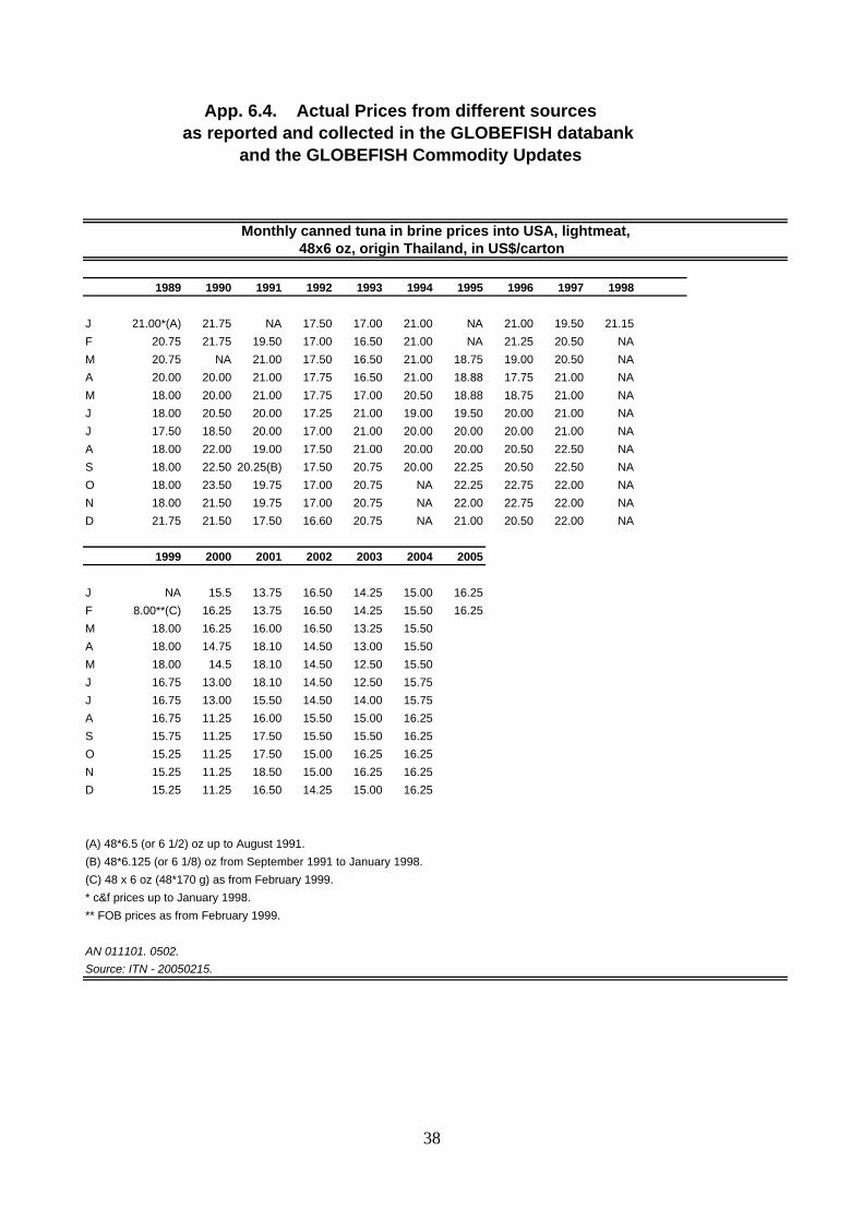
App. 6.4. Actual Prices from different sources as reported and collected in the GLOBEFISH databank

and the GLOBEFISH Commodity Updates

1989 1990 1991 1992 1993 1994 1995 1996 1997 1998

J 21.00*(A) 21.75 NA 17.50 17.00 21.00 NA 21.00 19.50 21.15

F 20.75 21.75 19.50 17.00 16.50 21.00 NA 21.25 20.50 NA

M 20.75 NA 21.00 17.50 16.50 21.00 18.75 19.00 20.50 NA

A 20.00 20.00 21.00 17.75 16.50 21.00 18.88 17.75 21.00 NA

M 18.00 20.00 21.00 17.75 17.00 20.50 18.88 18.75 21.00 NA

J 18.00 20.50 20.00 17.25 21.00 19.00 19.50 20.00 21.00 NA

J 17.50 18.50 20.00 17.00 21.00 20.00 20.00 20.00 21.00 NA

A 18.00 22.00 19.00 17.50 21.00 20.00 20.00 20.50 22.50 NA

S 18.00 22.50 20.25(B) 17.50 20.75 20.00 22.25 20.50 22.50 NA

O 18.00 23.50 19.75 17.00 20.75 NA 22.25 22.75 22.00 NA

N 18.00 21.50 19.75 17.00 20.75 NA 22.00 22.75 22.00 NA

D 21.75 21.50 17.50 16.60 20.75 NA 21.00 20.50 22.00 NA

1999 2000 2001 2002 2003 2004 2005

J NA 15.5 13.75 16.50 14.25 15.00 16.25

F 18.00**(C) 16.25 13.75 16.50 14.25 15.50 16.25

M 18.00 16.25 16.00 16.50 13.25 15.50

A 18.00 14.75 18.10 14.50 13.00 15.50

M 18.00 14.5 18.10 14.50 12.50 15.50

J 16.75 13.00 18.10 14.50 12.50 15.75

J 16.75 13.00 15.50 14.50 14.00 15.75

A 16.75 11.25 16.00 15.50 15.00 16.25

S 15.75 11.25 17.50 15.50 15.50 16.25

O 15.25 11.25 17.50 15.00 16.25 16.25

N 15.25 11.25 18.50 15.00 16.25 16.25

D 15.25 11.25 16.50 14.25 15.00 16.25

(A) 48*6.5 (or 6 1/2) oz up to August 1991.

(B) 48*6.125 (or 6 1/8) oz from September 1991 to January 1998.

(C) 48 x 6 oz (48*170 g) as from February 1999.

* c&f prices up to January 1998.

** FOB prices as from February 1999.

AN 011101. 0502.Source: ITN - 20050215.

Monthly canned tuna in brine prices into USA, lightmeat,48x6 oz, origin Thailand, in US$/carton

38

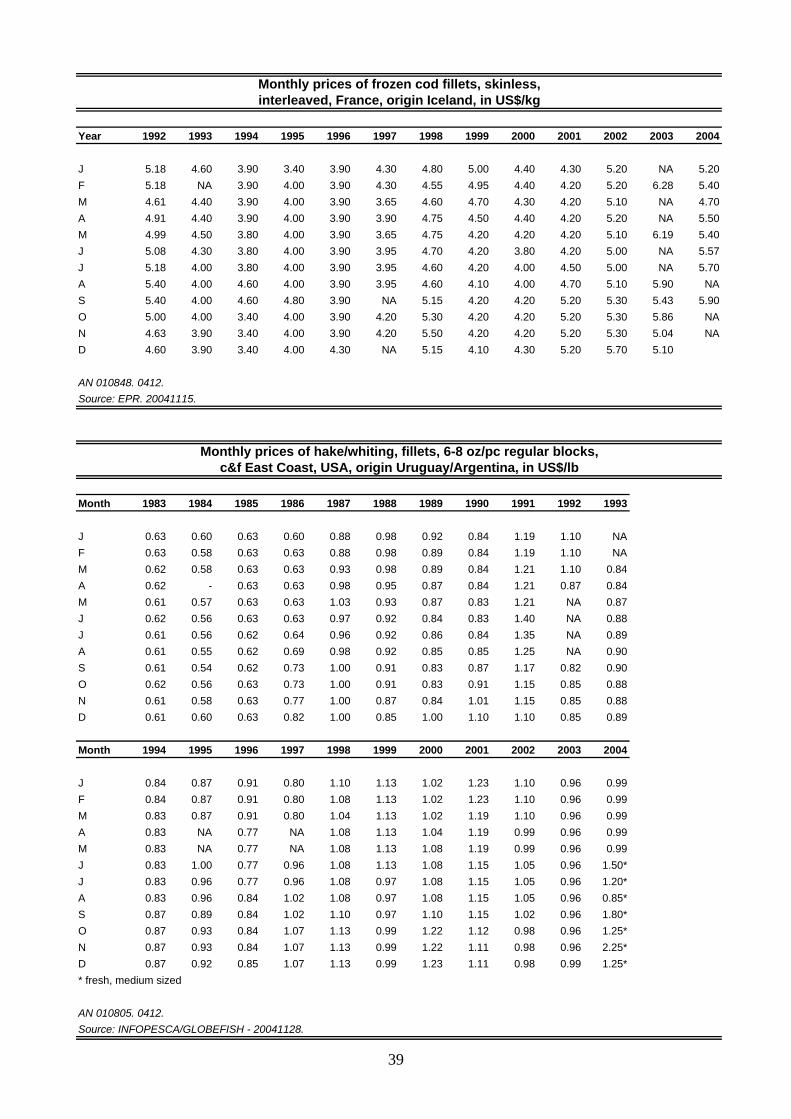
Year 1992 1993 1994 1995 1996 1997 1998 1999 2000 2001 2002 2003 2004

J 5.18 4.60 3.90 3.40 3.90 4.30 4.80 5.00 4.40 4.30 5.20 NA 5.20

F 5.18 NA 3.90 4.00 3.90 4.30 4.55 4.95 4.40 4.20 5.20 6.28 5.40

M 4.61 4.40 3.90 4.00 3.90 3.65 4.60 4.70 4.30 4.20 5.10 NA 4.70

A 4.91 4.40 3.90 4.00 3.90 3.90 4.75 4.50 4.40 4.20 5.20 NA 5.50

M 4.99 4.50 3.80 4.00 3.90 3.65 4.75 4.20 4.20 4.20 5.10 6.19 5.40

J 5.08 4.30 3.80 4.00 3.90 3.95 4.70 4.20 3.80 4.20 5.00 NA 5.57

J 5.18 4.00 3.80 4.00 3.90 3.95 4.60 4.20 4.00 4.50 5.00 NA 5.70

A 5.40 4.00 4.60 4.00 3.90 3.95 4.60 4.10 4.00 4.70 5.10 5.90 NA

S 5.40 4.00 4.60 4.80 3.90 NA 5.15 4.20 4.20 5.20 5.30 5.43 5.90

O 5.00 4.00 3.40 4.00 3.90 4.20 5.30 4.20 4.20 5.20 5.30 5.86 NA

N 4.63 3.90 3.40 4.00 3.90 4.20 5.50 4.20 4.20 5.20 5.30 5.04 NA

D 4.60 3.90 3.40 4.00 4.30 NA 5.15 4.10 4.30 5.20 5.70 5.10

Source: EPR. 20041115.

Month 1983 1984 1985 1986 1987 1988 1989 1990 1991 1992 1993

J 0.63 0.60 0.63 0.60 0.88 0.98 0.92 0.84 1.19 1.10 NA

F 0.63 0.58 0.63 0.63 0.88 0.98 0.89 0.84 1.19 1.10 NA

M 0.62 0.58 0.63 0.63 0.93 0.98 0.89 0.84 1.21 1.10 0.84

A 0.62 - 0.63 0.63 0.98 0.95 0.87 0.84 1.21 0.87 0.84

M 0.61 0.57 0.63 0.63 1.03 0.93 0.87 0.83 1.21 NA 0.87

J 0.62 0.56 0.63 0.63 0.97 0.92 0.84 0.83 1.40 NA 0.88

J 0.61 0.56 0.62 0.64 0.96 0.92 0.86 0.84 1.35 NA 0.89

A 0.61 0.55 0.62 0.69 0.98 0.92 0.85 0.85 1.25 NA 0.90

S 0.61 0.54 0.62 0.73 1.00 0.91 0.83 0.87 1.17 0.82 0.90

O 0.62 0.56 0.63 0.73 1.00 0.91 0.83 0.91 1.15 0.85 0.88

N 0.61 0.58 0.63 0.77 1.00 0.87 0.84 1.01 1.15 0.85 0.88

D 0.61 0.60 0.63 0.82 1.00 0.85 1.00 1.10 1.10 0.85 0.89

Month 1994 1995 1996 1997 1998 1999 2000 2001 2002 2003 2004

J 0.84 0.87 0.91 0.80 1.10 1.13 1.02 1.23 1.10 0.96 0.99

F 0.84 0.87 0.91 0.80 1.08 1.13 1.02 1.23 1.10 0.96 0.99

M 0.83 0.87 0.91 0.80 1.04 1.13 1.02 1.19 1.10 0.96 0.99

A 0.83 NA 0.77 NA 1.08 1.13 1.04 1.19 0.99 0.96 0.99

M 0.83 NA 0.77 NA 1.08 1.13 1.08 1.19 0.99 0.96 0.99

J 0.83 1.00 0.77 0.96 1.08 1.13 1.08 1.15 1.05 0.96 1.50*

J 0.83 0.96 0.77 0.96 1.08 0.97 1.08 1.15 1.05 0.96 1.20*

A 0.83 0.96 0.84 1.02 1.08 0.97 1.08 1.15 1.05 0.96 0.85*

S 0.87 0.89 0.84 1.02 1.10 0.97 1.10 1.15 1.02 0.96 1.80*

O 0.87 0.93 0.84 1.07 1.13 0.99 1.22 1.12 0.98 0.96 1.25*

N 0.87 0.93 0.84 1.07 1.13 0.99 1.22 1.11 0.98 0.96 2.25*

D 0.87 0.92 0.85 1.07 1.13 0.99 1.23 1.11 0.98 0.99 1.25*

* fresh, medium sized

AN 010805. 0412.Source: INFOPESCA/GLOBEFISH - 20041128.

Monthly prices of frozen cod fillets, skinless,interleaved, France, origin Iceland, in US$/kg

AN 010848. 0412.

Monthly prices of hake/whiting, fillets, 6-8 oz/pc regular blocks,c&f East Coast, USA, origin Uruguay/Argentina, in US$/lb

39

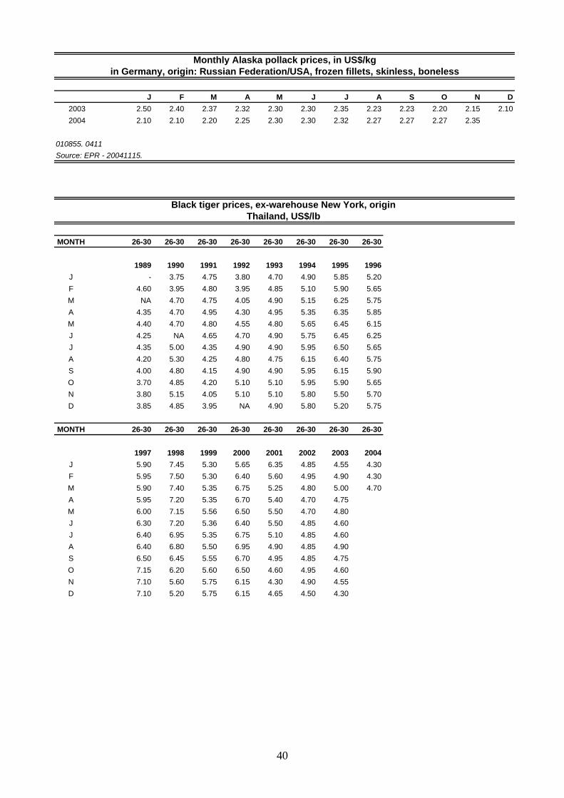
J F M A M J J A S O N D

2003 2.50 2.40 2.37 2.32 2.30 2.30 2.35 2.23 2.23 2.20 2.15 2.10

2004 2.10 2.10 2.20 2.25 2.30 2.30 2.32 2.27 2.27 2.27 2.35

Source: EPR - 20041115.

MONTH 26-30 26-30 26-30 26-30 26-30 26-30 26-30 26-30

1989 1990 1991 1992 1993 1994 1995 1996

J - 3.75 4.75 3.80 4.70 4.90 5.85 5.20

F 4.60 3.95 4.80 3.95 4.85 5.10 5.90 5.65

M NA 4.70 4.75 4.05 4.90 5.15 6.25 5.75

A 4.35 4.70 4.95 4.30 4.95 5.35 6.35 5.85

M 4.40 4.70 4.80 4.55 4.80 5.65 6.45 6.15

J 4.25 NA 4.65 4.70 4.90 5.75 6.45 6.25

J 4.35 5.00 4.35 4.90 4.90 5.95 6.50 5.65

A 4.20 5.30 4.25 4.80 4.75 6.15 6.40 5.75

S 4.00 4.80 4.15 4.90 4.90 5.95 6.15 5.90

O 3.70 4.85 4.20 5.10 5.10 5.95 5.90 5.65

N 3.80 5.15 4.05 5.10 5.10 5.80 5.50 5.70

D 3.85 4.85 3.95 NA 4.90 5.80 5.20 5.75

MONTH 26-30 26-30 26-30 26-30 26-30 26-30 26-30 26-30

1997 1998 1999 2000 2001 2002 2003 2004

J 5.90 7.45 5.30 5.65 6.35 4.85 4.55 4.30

F 5.95 7.50 5.30 6.40 5.60 4.95 4.90 4.30

M 5.90 7.40 5.35 6.75 5.25 4.80 5.00 4.70

A 5.95 7.20 5.35 6.70 5.40 4.70 4.75

M 6.00 7.15 5.56 6.50 5.50 4.70 4.80

J 6.30 7.20 5.36 6.40 5.50 4.85 4.60

J 6.40 6.95 5.35 6.75 5.10 4.85 4.60

A 6.40 6.80 5.50 6.95 4.90 4.85 4.90

S 6.50 6.45 5.55 6.70 4.95 4.85 4.75

O 7.15 6.20 5.60 6.50 4.60 4.95 4.60

N 7.10 5.60 5.75 6.15 4.30 4.90 4.55

D 7.10 5.20 5.75 6.15 4.65 4.50 4.30

Monthly Alaska pollack prices, in US$/kgin Germany, origin: Russian Federation/USA, frozen fillets, skinless, boneless

010855. 0411

Black tiger prices, ex-warehouse New York, origin Thailand, US$/lb

40

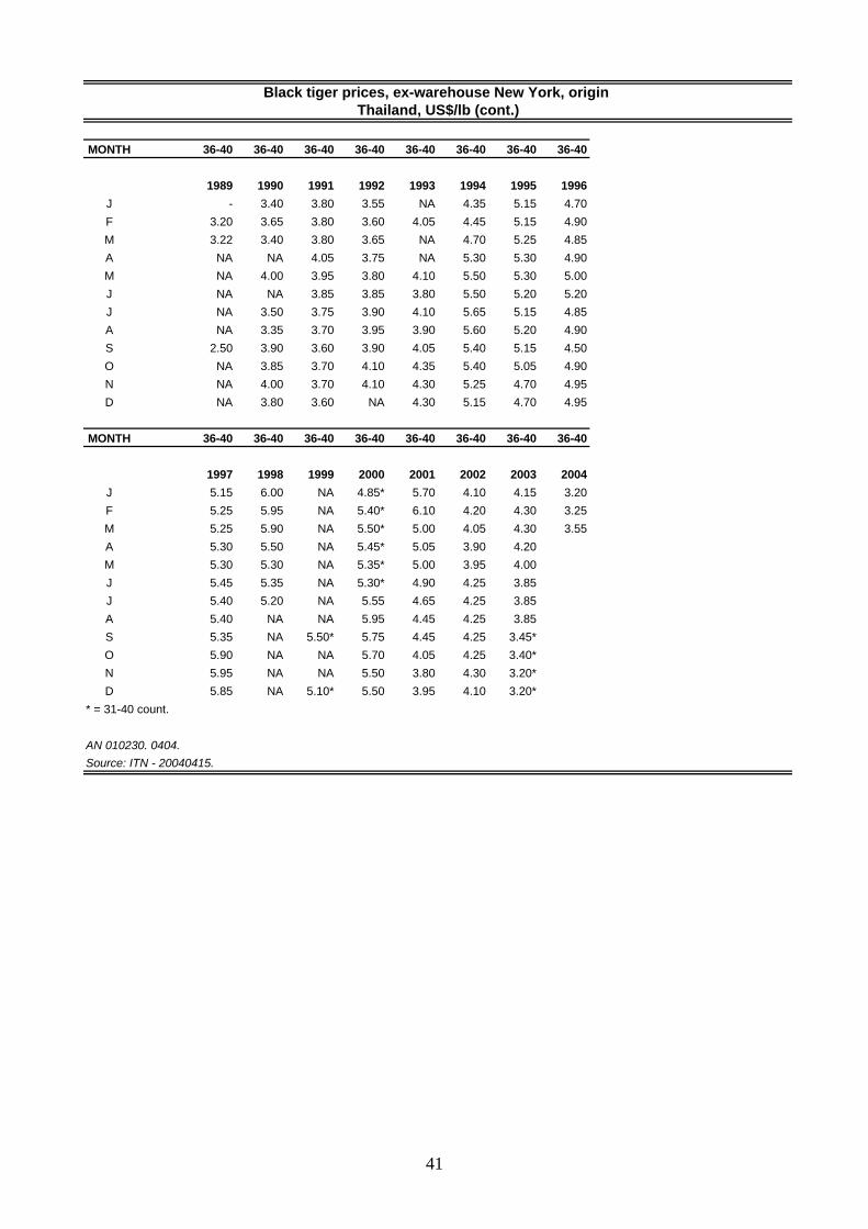
MONTH 36-40 36-40 36-40 36-40 36-40 36-40 36-40 36-40

1989 1990 1991 1992 1993 1994 1995 1996

J - 3.40 3.80 3.55 NA 4.35 5.15 4.70

F 3.20 3.65 3.80 3.60 4.05 4.45 5.15 4.90

M 3.22 3.40 3.80 3.65 NA 4.70 5.25 4.85

A NA NA 4.05 3.75 NA 5.30 5.30 4.90

M NA 4.00 3.95 3.80 4.10 5.50 5.30 5.00

J NA NA 3.85 3.85 3.80 5.50 5.20 5.20

J NA 3.50 3.75 3.90 4.10 5.65 5.15 4.85

A NA 3.35 3.70 3.95 3.90 5.60 5.20 4.90

S 2.50 3.90 3.60 3.90 4.05 5.40 5.15 4.50

O NA 3.85 3.70 4.10 4.35 5.40 5.05 4.90

N NA 4.00 3.70 4.10 4.30 5.25 4.70 4.95

D NA 3.80 3.60 NA 4.30 5.15 4.70 4.95

MONTH 36-40 36-40 36-40 36-40 36-40 36-40 36-40 36-40

1997 1998 1999 2000 2001 2002 2003 2004

J 5.15 6.00 NA 4.85* 5.70 4.10 4.15 3.20

F 5.25 5.95 NA 5.40* 6.10 4.20 4.30 3.25

M 5.25 5.90 NA 5.50* 5.00 4.05 4.30 3.55

A 5.30 5.50 NA 5.45* 5.05 3.90 4.20

M 5.30 5.30 NA 5.35* 5.00 3.95 4.00

J 5.45 5.35 NA 5.30* 4.90 4.25 3.85

J 5.40 5.20 NA 5.55 4.65 4.25 3.85

A 5.40 NA NA 5.95 4.45 4.25 3.85

S 5.35 NA 5.50* 5.75 4.45 4.25 3.45*

O 5.90 NA NA 5.70 4.05 4.25 3.40*

N 5.95 NA NA 5.50 3.80 4.30 3.20*

D 5.85 NA 5.10* 5.50 3.95 4.10 3.20*

* = 31-40 count.

AN 010230. 0404.Source: ITN - 20040415.

Black tiger prices, ex-warehouse New York, origin Thailand, US$/lb (cont.)

41

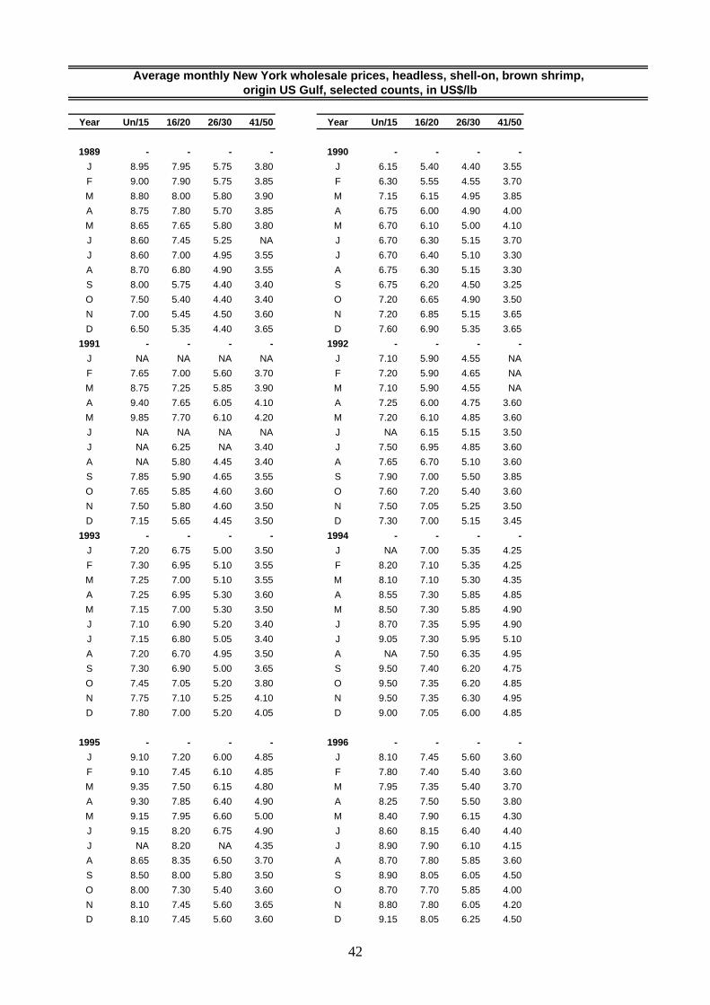
Year Un/15 16/20 26/30 41/50 Year Un/15 16/20 26/30 41/50

1989 - - - - 1990 - - - -

J 8.95 7.95 5.75 3.80 J 6.15 5.40 4.40 3.55

F 9.00 7.90 5.75 3.85 F 6.30 5.55 4.55 3.70

M 8.80 8.00 5.80 3.90 M 7.15 6.15 4.95 3.85

A 8.75 7.80 5.70 3.85 A 6.75 6.00 4.90 4.00

M 8.65 7.65 5.80 3.80 M 6.70 6.10 5.00 4.10

J 8.60 7.45 5.25 NA J 6.70 6.30 5.15 3.70

J 8.60 7.00 4.95 3.55 J 6.70 6.40 5.10 3.30

A 8.70 6.80 4.90 3.55 A 6.75 6.30 5.15 3.30

S 8.00 5.75 4.40 3.40 S 6.75 6.20 4.50 3.25

O 7.50 5.40 4.40 3.40 O 7.20 6.65 4.90 3.50

N 7.00 5.45 4.50 3.60 N 7.20 6.85 5.15 3.65

D 6.50 5.35 4.40 3.65 D 7.60 6.90 5.35 3.65

1991 - - - - 1992 - - - -

J NA NA NA NA J 7.10 5.90 4.55 NA

F 7.65 7.00 5.60 3.70 F 7.20 5.90 4.65 NA

M 8.75 7.25 5.85 3.90 M 7.10 5.90 4.55 NA

A 9.40 7.65 6.05 4.10 A 7.25 6.00 4.75 3.60

M 9.85 7.70 6.10 4.20 M 7.20 6.10 4.85 3.60

J NA NA NA NA J NA 6.15 5.15 3.50

J NA 6.25 NA 3.40 J 7.50 6.95 4.85 3.60

A NA 5.80 4.45 3.40 A 7.65 6.70 5.10 3.60

S 7.85 5.90 4.65 3.55 S 7.90 7.00 5.50 3.85

O 7.65 5.85 4.60 3.60 O 7.60 7.20 5.40 3.60

N 7.50 5.80 4.60 3.50 N 7.50 7.05 5.25 3.50

D 7.15 5.65 4.45 3.50 D 7.30 7.00 5.15 3.45

1993 - - - - 1994 - - - -

J 7.20 6.75 5.00 3.50 J NA 7.00 5.35 4.25

F 7.30 6.95 5.10 3.55 F 8.20 7.10 5.35 4.25

M 7.25 7.00 5.10 3.55 M 8.10 7.10 5.30 4.35

A 7.25 6.95 5.30 3.60 A 8.55 7.30 5.85 4.85

M 7.15 7.00 5.30 3.50 M 8.50 7.30 5.85 4.90

J 7.10 6.90 5.20 3.40 J 8.70 7.35 5.95 4.90

J 7.15 6.80 5.05 3.40 J 9.05 7.30 5.95 5.10

A 7.20 6.70 4.95 3.50 A NA 7.50 6.35 4.95

S 7.30 6.90 5.00 3.65 S 9.50 7.40 6.20 4.75

O 7.45 7.05 5.20 3.80 O 9.50 7.35 6.20 4.85

N 7.75 7.10 5.25 4.10 N 9.50 7.35 6.30 4.95

D 7.80 7.00 5.20 4.05 D 9.00 7.05 6.00 4.85

1995 - - - - 1996 - - - -

J 9.10 7.20 6.00 4.85 J 8.10 7.45 5.60 3.60

F 9.10 7.45 6.10 4.85 F 7.80 7.40 5.40 3.60

M 9.35 7.50 6.15 4.80 M 7.95 7.35 5.40 3.70

A 9.30 7.85 6.40 4.90 A 8.25 7.50 5.50 3.80

M 9.15 7.95 6.60 5.00 M 8.40 7.90 6.15 4.30

J 9.15 8.20 6.75 4.90 J 8.60 8.15 6.40 4.40

J NA 8.20 NA 4.35 J 8.90 7.90 6.10 4.15

A 8.65 8.35 6.50 3.70 A 8.70 7.80 5.85 3.60

S 8.50 8.00 5.80 3.50 S 8.90 8.05 6.05 4.50

O 8.00 7.30 5.40 3.60 O 8.70 7.70 5.85 4.00

N 8.10 7.45 5.60 3.65 N 8.80 7.80 6.05 4.20D 8.10 7.45 5.60 3.60 D 9.15 8.05 6.25 4.50

Average monthly New York wholesale prices, headless, shell-on, brown shrimp, origin US Gulf, selected counts, in US$/lb

42

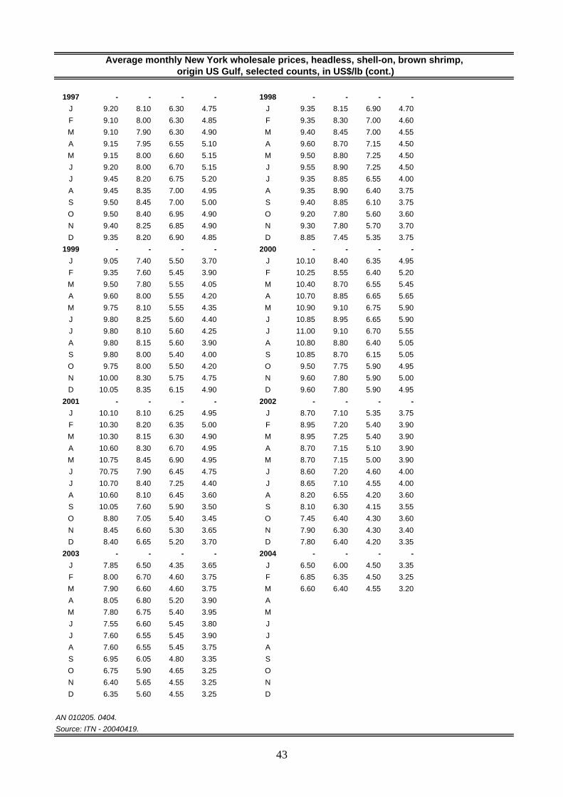
1997 - - - - 1998 - - - -

J 9.20 8.10 6.30 4.75 J 9.35 8.15 6.90 4.70

F 9.10 8.00 6.30 4.85 F 9.35 8.30 7.00 4.60

M 9.10 7.90 6.30 4.90 M 9.40 8.45 7.00 4.55

A 9.15 7.95 6.55 5.10 A 9.60 8.70 7.15 4.50

M 9.15 8.00 6.60 5.15 M 9.50 8.80 7.25 4.50

J 9.20 8.00 6.70 5.15 J 9.55 8.90 7.25 4.50

J 9.45 8.20 6.75 5.20 J 9.35 8.85 6.55 4.00

A 9.45 8.35 7.00 4.95 A 9.35 8.90 6.40 3.75

S 9.50 8.45 7.00 5.00 S 9.40 8.85 6.10 3.75

O 9.50 8.40 6.95 4.90 O 9.20 7.80 5.60 3.60

N 9.40 8.25 6.85 4.90 N 9.30 7.80 5.70 3.70

D 9.35 8.20 6.90 4.85 D 8.85 7.45 5.35 3.75

1999 - - - - 2000 - - - -

J 9.05 7.40 5.50 3.70 J 10.10 8.40 6.35 4.95

F 9.35 7.60 5.45 3.90 F 10.25 8.55 6.40 5.20

M 9.50 7.80 5.55 4.05 M 10.40 8.70 6.55 5.45

A 9.60 8.00 5.55 4.20 A 10.70 8.85 6.65 5.65

M 9.75 8.10 5.55 4.35 M 10.90 9.10 6.75 5.90

J 9.80 8.25 5.60 4.40 J 10.85 8.95 6.65 5.90

J 9.80 8.10 5.60 4.25 J 11.00 9.10 6.70 5.55

A 9.80 8.15 5.60 3.90 A 10.80 8.80 6.40 5.05

S 9.80 8.00 5.40 4.00 S 10.85 8.70 6.15 5.05

O 9.75 8.00 5.50 4.20 O 9.50 7.75 5.90 4.95

N 10.00 8.30 5.75 4.75 N 9.60 7.80 5.90 5.00

D 10.05 8.35 6.15 4.90 D 9.60 7.80 5.90 4.95

2001 - - - - 2002 - - - -

J 10.10 8.10 6.25 4.95 J 8.70 7.10 5.35 3.75

F 10.30 8.20 6.35 5.00 F 8.95 7.20 5.40 3.90

M 10.30 8.15 6.30 4.90 M 8.95 7.25 5.40 3.90

A 10.60 8.30 6.70 4.95 A 8.70 7.15 5.10 3.90

M 10.75 8.45 6.90 4.95 M 8.70 7.15 5.00 3.90

J 70.75 7.90 6.45 4.75 J 8.60 7.20 4.60 4.00

J 10.70 8.40 7.25 4.40 J 8.65 7.10 4.55 4.00

A 10.60 8.10 6.45 3.60 A 8.20 6.55 4.20 3.60

S 10.05 7.60 5.90 3.50 S 8.10 6.30 4.15 3.55

O 8.80 7.05 5.40 3.45 O 7.45 6.40 4.30 3.60

N 8.45 6.60 5.30 3.65 N 7.90 6.30 4.30 3.40

D 8.40 6.65 5.20 3.70 D 7.80 6.40 4.20 3.35

2003 - - - - 2004 - - - -

J 7.85 6.50 4.35 3.65 J 6.50 6.00 4.50 3.35

F 8.00 6.70 4.60 3.75 F 6.85 6.35 4.50 3.25

M 7.90 6.60 4.60 3.75 M 6.60 6.40 4.55 3.20

A 8.05 6.80 5.20 3.90 A

M 7.80 6.75 5.40 3.95 M

J 7.55 6.60 5.45 3.80 J

J 7.60 6.55 5.45 3.90 J

A 7.60 6.55 5.45 3.75 A

S 6.95 6.05 4.80 3.35 S

O 6.75 5.90 4.65 3.25 O

N 6.40 5.65 4.55 3.25 N

D 6.35 5.60 4.55 3.25 D

AN 010205. 0404.Source: ITN - 20040419.

Average monthly New York wholesale prices, headless, shell-on, brown shrimp, origin US Gulf, selected counts, in US$/lb (cont.)

43

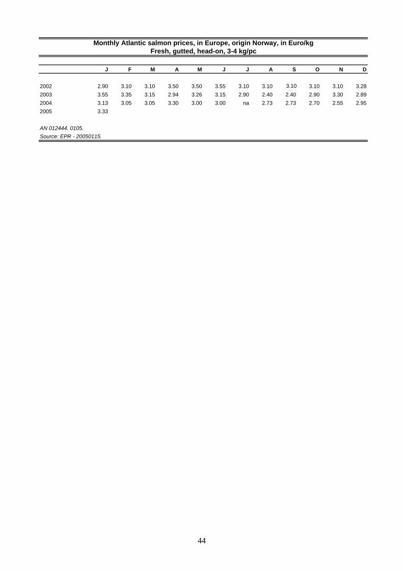
J F M A M J J A S O N D

2002 2.90 3.10 3.10 3.50 3.50 3.55 3.10 3.10 3.10 3.10 3.10 3.28

2003 3.55 3.35 3.15 2.94 3.26 3.15 2.90 2.40 2.40 2.90 3.30 2.89

2004 3.13 3.05 3.05 3.30 3.00 3.00 na 2.73 2.73 2.70 2.55 2.95

2005 3.33

AN 012444. 0105.Source: EPR - 20050115.

Monthly Atlantic salmon prices, in Europe, origin Norway, in Euro/kgFresh, gutted, head-on, 3-4 kg/pc

44

GLOBEFISH MARKET RESEARCH PROGRAMME

This activity is part of the services provided by the Fish Marketing and Utilization Service (FIIU) of the Fisheries Department of the Food and Agriculture Organization of the United Nations.

Issued

Language

€

No. of copies

Vol.63 The World Market for Herring (96p.)................................................. ..... Mar 2000 Eng 30 --

Vol.64 World Trade in Mackerel and Horse Mackerel (98p.).........................……….April 2000 Eng 30 --

Vol.65 Effect of World Trade Organization’s Regulation on World Fish Trade (87p.)…..Mar 2000 Eng 30 --

Vol.66 European Union Standards for Fishery Products (including EU duties) (248p.)…..June 2000 Eng 30 --

Vol.67 The Ornamental Fish Market (91p.)..........................................................Oct 2000 Eng 30 --

Vol.68 The World Market for Frog Legs (44p.) ........................................... …… ..June 2001 Eng 30 --

Vol.69 Fishery Industry Profile – Thailand (76p.) ................................................ Nov 2001 Eng 30 --

Vol.70 The Fishery Industry in Greece (59p.)...................................................... Nov 2001 Eng 30 --

Vol.71 The German Market for Fish and Seafood (116p.)........................................ Jan 2002 Eng 30 --

Vol.72 Fish Roe in Europe: Supply and Demand Conditions (47p.).......................... …Nov 2002 Eng 30 --

Vol.73 Salmon – A Study of Global Supply and Demand (151p.).……………………….. …. July 2003 Eng 30 --

Vol.74 World Tuna markets (135p.)...................................................................May 2004 Eng 30 --

Vol.75 Fishery Industry Profile – Viet Nam (57p.)..................................................July 2004 Eng 30 --

Vol.76 Fishery Industry in China (74p.)...............................................................Sept 2004 Eng 30 --

Vol.77 Overview of Organic Markets: an Opportunity for Aquaculture Products?(98p.).....Jan 2005 Eng 30 --

Vol.78 Seafood Price Indices (44p.).…………………………………………………………………Apr 2005 Eng 30 --

1) Prices include air mail delivery

……………………………………………………………………………………………………………………………………………………. ORDER FORM

COPIES ARE AVAILABLE FROM:

FAO GLOBEFISH - Fish Utilization and Marketing Service, Fishery Industries Division Viale delle Terme di Caracalla, 00100 Rome, Italy Tel.: (39-06)570 56313 - Fax: (39-06) 570 55188 - E-mail: GLOBEFISH@fao.org – http//:www.globefish.org 20% DISCOUNT IS OFFERED ON ORDERS FOR MORE THAN TWO COPIES I should like to order _____ copy(ies) of those volume number(s) as indicated above for a total of € _____ ? By bank cheque/draft in € __________ payable to GLOBEFISH (see address above) ? By credit card: Card No.: ____________________________________ ? Diners/Visa ? Euro/Master Card ? American Express Expiry date: __________________________________ Signature: ____________________________ ? Bank transfer to: FAO/UN Trust Fund US$ Account 490650/67/72 with the IntesaBCI, FAO Branch (Swift Code BCIT IT MM 700), ABI: 03069, CAB: 03356; IBAN IT24N03693356004906507681; Viale delle Terme di Caracalla – 00100 Rome, making reference to FAO Account Code TFAA970089102 (GLOBEFISH) for € _________________ Name: ______________________________________ Company: _______________________________________

Street Address: _________________________________________________________________________________________

City and Postcode: ______________________________ Country: ________________________________________

Tel:_____________________Fax: _________________ E-mail: _________________________________________

GLOBEFISH RESEARCH PROGRAMME

Food and Agriculture Organization of the United NationsFishery Industries Division

Viale delle Terme di Caracalla00100 Rome, Italy

Tel.: +39 06 5705 5074Fax: +39 06 5705 5188

www.globefish.org

Seafood Price Indices

Volume 78