Technical Report NOS CO-OPS 053

SEA LEVEL VARIATIONS OF THE UNITED STATES 1854-2006

Silver Spring, Maryland December 2009

noaa National Oceanic and Atmospheric Administration

U.S. DEPARTMENT OF COMMERCE National Ocean Service Center for Operational Oceanographic Products and Services

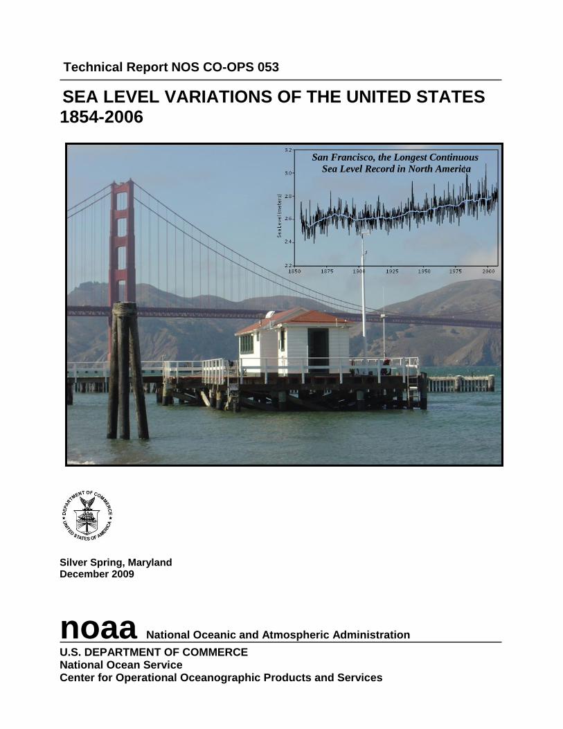
San Francisco, the Longest Continuous

Sea Level Record in North America

Center for Operational Oceanographic Products and Services

National Ocean Service

National Oceanic and Atmospheric Administration

U.S. Department of Commerce

The National Ocean Service (NOS) Center for Operational Oceanographic Products and Services

(CO-OPS) provides the National infrastructure, science, and technical expertise to collect and

distribute observations and predictions of water levels and currents to ensure safe, efficient and

environmentally sound maritime commerce. The Center provides the set of water level and tidal

current products required to support NOS’ Strategic Plan mission requirements, and to assist in

providing operational oceanographic data/products required by NOAA’s other Strategic Plan

themes. For example, CO-OPS provides data and products required by the National Weather Service

to meet its flood and tsunami warning responsibilities. The Center manages the National Water

Level Observation Network (NWLON), a national network of Physical Oceanographic Real-Time

Systems (PORTS) in major U. S. harbors, and the National Current Observation Program consisting

of current surveys in near shore and coastal areas utilizing bottom mounted platforms, subsurface

buoys, horizontal sensors and quick response real time buoys. The Center: establishes standards for

the collection and processing of water level and current data; collects and documents user

requirements which serve as the foundation for all resulting program activities; designs new and/or

improved oceanographic observing systems; designs software to improve CO-OPS’ data processing

capabilities; maintains and operates oceanographic observing systems; performs operational data

analysis/quality control; and produces/disseminates oceanographic products.

Cover photo of the San Francisco Sea Level Station maintained by NOAA’s Center for Operational Oceanographic

Products and Services.

NOAA Technical Report NOS CO-OPS 053

SEA LEVEL VARIATIONS OF THE UNITED STATES 1854-2006

Chris Zervas

December 2009

U.S. DEPARTMENT OF COMMERCE Gary Locke, SecretaryNational Oceanic and Atmospheric Administration

Dr. Jane Lubchenco, Undersecretary of Commerce for Oceans and Atmosphere and NOAA Administrator National Ocean Service John H. Dunnigan, Assistant Administrator

Center for Operational Oceanographic Products and Services Michael Szabados, Director

NOTICE

Mention of a commercial company or product does not constitute an

endorsement by NOAA. Use for publicity or advertising purposes of

information from this publication concerning proprietary products or the

results of the tests of such products is not authorized.

iii

FOREWARD

The United States National Water Level Network (NWLON) was established in the 19th

Century to ensure the Nation’s nautical charts, shoreline maps, and elevations relative to homes,

levees, and other coastal infrastructure were accurately referenced to sea level. In support of this

mission, NOAA’s Center for Operational Oceanographic Products and Services and its

predecessors have determined sea level for the United States since the mid 19th

Century. While

climate change was not a concern during the mid-1800s, the accurate determination of sea level

was critical for navigation and marine boundary determination. To meet these important

requirements, technology, procedures, and processes were developed to the highest scientific and

engineering standards.

At the turn of the 20th

Century it was realized that there was a need to account for a rise in

sea level and the first National Tidal Datum Epoch was established. Today this Epoch is updated

every 20 to 25 years. The Supreme Court recognized these standards and procedures in the

landmark 1936 case of Borax, Ltd v. City of Los Angeles when legally defining sea level. Due to

those initial efforts and the continued dedication of those charged with the responsibility for

monitoring sea level for the United States, we can accurately determine relative (local) mean sea

level along the Nation’s coastline today. These observations also play an important role in

monitoring change in global sea level.

As we monitor change in sea level into the 21st Century, the statement made by Alexander

Dallas Bache, the Second Superintendent of the Coast Survey, is as relevant today as when it was

stated more than 150 years ago, “It seems a very simple task to make correct tidal observations;

but, in all my experience, I have found no observations which require such constant care and

attention” (1854).

Michael Szabados

Director, Center for Operational Oceanographic Products and Services

iv

v

TABLE OF CONTENTS

FOREWARD ............................................................................................................................ iii

LIST OF FIGURES .................................................................................................................. vii

LIST OF TABLES .................................................................................................................... ix

LIST OF ACRONYMS ............................................................................................................ xi

EXECUTIVE SUMMARY ...................................................................................................... xiiii

INTRODUCTION .................................................................................................................... 1

WATER LEVEL STATIONS .................................................................................................. 5

DERIVATION OF MEAN SEA LEVEL TRENDS ................................................................ 15

LINEAR MEAN SEA LEVEL TRENDS ................................................................................ 19

AVERAGE SEASONAL MEAN SEA LEVEL CYCLE ........................................................ 37

VARIABILITY OF RESIDUAL MONTHLY MEAN SEA LEVEL ...................................... 47

DISCUSSION ........................................................................................................................... 59

CONCLUSION ......................................................................................................................... 67

ACKNOWLEDGMENTS ........................................................................................................ 71

REFERENCES ......................................................................................................................... 73

APPENDICES .......................................................................................................................... 77

APPENDIX I. National Water Level Observation Network Stations ............................ A-1

APPENDIX II. Time series of monthly mean sea level after removal of the average

seasonal cycle showing the derived linear trend .............................................................. B-1

APPENDIX III. Average seasonal cycle of monthly mean sea level with 95% confidence

intervals ............................................................................................................................ C-1

APPENDIX IV. Comparison of Sa and Ssa tidal constituents derived from average

seasonal cycles with the accepted tidal constituents used for CO-OPS tide predictions . D-1

APPENDIX V. Linear trends for 50-year periods of mean sea level data ..................... E-1

vi

vii

LIST OF FIGURES

Figure 1. Long-term NWLON stations on the U.S. east coast and Bermuda ................................ 9

Figure 2. Long-term NWLON stations on the U.S. west coast with major earthquake indicated

by its magnitude. ........................................................................................................................... 10

Figure 3. Long-term NWLON stations in the eastern Gulf of Mexico and Caribbean. .............. 11

Figure 4. Long-term NWLON stations in the western Gulf of Mexico....................................... 11

Figure 5. Long-term NWLON stations in Alaska with major earthquakes indicated by

magnitude. ..................................................................................................................................... 12

Figure 6. Long-term NWLON stations in the eastern Pacific with major earthquake indicated by

its magnitude. ................................................................................................................................ 12

Figure 7. . Long-term NWLON stations in the western Pacific with major earthquake indicated

by its magnitude. ........................................................................................................................... 13

Figure 8. Partial autocorrelation functions of residual time series versus lag in months. Values

above or ......................................................................................................................................... 16

Figure 9. MSL trends with 95% confidence intervals (mm/yr) for all monthly data up to 2006 for

U.S. east coast stations. ................................................................................................................. 25

Figure 10. MSL trends with 95% confidence intervals (mm/yr) for all monthly data up to 2006

for U.S. west coast stations and Alaska. ....................................................................................... 26

Figure 11. MSL trends and 95% confidence intervals (mm/yr) for all monthly data up to 2006 for

Gulf of Mexico, tropical Pacific, Bermuda, and Caribbean stations. ........................................... 27

Figure 12. Autoregressive coefficient with 95% confidence interval for U.S. east coast stations. .. 28

Figure 13. Autoregressive coefficient with 95% confidence interval for U.S. west coast and

Alaska stations. ............................................................................................................................. 29

Figure 14. Autoregressive coefficient with 95% confidence interval for Gulf of Mexico, tropical

Pacific, Bermuda, and Caribbean stations. ................................................................................... 30

Figure 15. Monthly MSL data for Yakutat after removal of the average seasonal cycle.

Calculated trends are shown with 95% confidence intervals. Possible MSL trends for Yakutat

are a) a single trend of -6.44 +/- 0.47 mm/yr or b) a February 1979 offset and change in trend

from -4.81 +/- 0.89 mm/yr to -11.53 +/- 1.46 mm/yr. .................................................................. 32

Figure 16. Monthly MSL data for Freeport after removal of the average seasonal cycle. The

trend of 4.35 +/- 1.12 mm/yr was calculated with an apparent datum shift of 0.190 m on January

1972 and is shown with its 95% confidence interval. ................................................................... 33

Figure 17. Monthly MSL data for San Francisco after removal of the average seasonal cycle.

The trends before and after an apparent datum shift of 0.075 m on September 1897 are 2.05 +/-

0.85 mm/yr and 2.01 +/- 0.21 mm/yr. The time of the April 1906 earthquake is shown by the

solid vertical line. .......................................................................................................................... 34

Figure 18. Monthly MSL data for San Francisco after removal of the average seasonal cycle and

removal of an apparent datum shift of 0.037 m on September 1897. The total trend is 1.73 +/-

0.13 mm/yr. The time of the April 1906 earthquake is shown by the solid vertical line............. 35

viii

Figure 19. Monthly MSL data for Sausalito after removal of the average seasonal cycle. The

total trend is 0.96 +/- 0.54 mm/yr. The time of the April 1906 earthquake is shown by the solid

vertical line.................................................................................................................................... 36

Figure 20. Comparison of derived and accepted long-term tidal constituent amplitudes (top) and

phases (bottom) for northern U.S. east coast stations. .................................................................. 40

Figure 21. Comparison of derived and accepted long-term tidal constituent amplitudes (top) and

phases (bottom) for southern U.S. east coast stations. .................................................................. 41

Figure 22. Comparison of derived and accepted long-term tidal constituent amplitudes (top) and

phases (bottom) for southern U.S. west coast stations.................................................................. 42

Figure 23. Comparison of derived and accepted long-term tidal constituent amplitudes (top) and

phases (bottom) for northern U.S. west coast and Alaska stations. .............................................. 43

Figure 24. Comparison of derived and accepted long-term tidal constituent amplitudes (top) and

phases (bottom) for Gulf of Mexico stations. ............................................................................... 44

Figure 25. Comparison of derived and accepted long-term tidal constituent amplitudes (top) and

phases (bottom) for tropical Pacific, Bermuda, and Caribbean stations. ...................................... 45

Figure 26. Comparison between the monthly mean sea level residual for San Diego (solid line)

and the Oceanic Niño Index (dashed line). The ONI has been divided by a factor of 10 to show

the correlation; its units are in degrees. ........................................................................................ 49

Figure 27. Comparison between the monthly mean sea level residual for Kwajalein (solid line)

and the Oceanic Niño Index (dashed line). The ONI has been divided by a factor of 10 to show

the correlation; its units are in degrees. ........................................................................................ 49

Figure 28. +/- 95% confidence interval of linear MSL trends (mm/yr) versus year range of data. 59

Figure 29. +/- 95% confidence interval of linear MSL trends (mm/yr) versus year range of data.

The least squares fitted line is also shown. ................................................................................... 60

Figure 30. 95% confidence interval for linear MSL trend (mm/yr) versus year range of data

based on equation 8. ...................................................................................................................... 61

Figure 31. 50-year MSL trends with 95% confidence intervals at The Battery. Horizontal line is

the MSL trend from all the data since 1856 (2.77 +/- 0.09 mm/yr). ............................................. 62

Figure 32. San Francisco 50-year MSL trends with 95% confidence intervals for the (a) original

time series and (b) adjusted time series. Horizontal line is the MSL trend from all the data since

1897 (2.01 +/- 0.21 mm/yr). ......................................................................................................... 63

Figure 33. Mean sea level for 2002-2006 relative to the 1983-2001 MSL datum for stations that

have not been updated to a 5-year MSL datum due to rapid relative sea level trends. ................. 65

Figure 34. Estimated absolute MSL change for 12 and 22 years after the establishment of an

NTDE as a function of the rate of sea level change. ..................................................................... 66

Figure 35. Comparison of the atmospheric carbon dioxide record at Mauna Loa, Hawaii since

1958 (from http://www.esrl.noaa.gov/gmd/ccgg/trends/co2_data_mlo.html ) and monthly mean

sea levels at eight NWLON stations with record lengths of over 100 years. ............................... 69

ix

LIST OF TABLES

Table 1. Major Earthquakes near NWLON Stations ...................................................................... 5

Table 2. Combined Stations ............................................................................................................ 7

Table 3. Effect of serial correlation of time series residuals on standard errors ........................... 17

Table 4. Linear MSL trends for all monthly data up to 2006 ....................................................... 21

Table 5. Periods of suspect data .................................................................................................... 47

Table 6. Number of months with extreme residual water levels for Atlantic stations. ................. 51

Table 7. Number of months with extreme residual water levels for Pacific stations. .................. 55

x

xi

LIST OF ACRONYMS

CO-OPS Center for Operational Oceanographic Products and Services

ENSO El Niño/Southern Oscillation

MSL Mean Sea Level

MTDE Modified Tidal Datum Epoch

NOAA National Oceanographic and Atmospheric Administration

NOS National Ocean Service

NTDE National Tidal Datum Epoch

NWLON National Water Level Observation Network

TCOON Texas Coastal Ocean Observation Network

xii

xiii

EXECUTIVE SUMMARY

Monthly mean sea level (MSL) data for 128 long-term National Water Level Observation

Network (NWLON) stations of the Center for Operational Oceanographic Products and Services

(CO-OPS) are analyzed in this report. All available data up to the end of 2006 are used to

determine linear trends, average seasonal cycles, and interannual variability including estimated

errors. The stations are located on the U.S. Atlantic and Pacific coasts, the Gulf of Mexico,

Hawaii, Alaska, and on islands in the Atlantic and Pacific Oceans.

The linear trends obtained are relative MSL trends which are a combination of the absolute

global rate of sea level rise (1.7 +/- 0.5 mm/yr in the 20th

century) and the rate of any local

vertical land motion. The variation in vertical land motion, ranging from rapid subsidence in

Louisiana and eastern Texas to rapid uplift in Alaska, is primarily responsible for the regional

differences in MSL trends and for the differing rates within regions. Separate pre- and post-

seismic trends were calculated for some stations in Alaska and Guam with apparent seismic

offsets in 1957, 1964, or 1993.

Time series plots of the monthly MSL data with the seasonal cycle removed are located in the

appendices along with the 12-month average seasonal cycle for each station. The average

seasonal cycles are used to derive the two tidal constituents that represent the regular seasonal

variation which are then compared to the tidal constituents routinely used by CO-OPS to make

the official tide predictions. The residual time series after the seasonal cycles and trends are

removed represent the regional oceanic interannual variability, which is highly correlated from

station to station. Using a 5-month running average of the residual, thresholds of +0.1 and -0.1

meters are defined for positive and negative anomalies.

Each calculated linear trend has an associated 95% confidence interval that is primarily

dependent on the year range of data for each station. A derived inverse power relationship

indicates that 50-60 years of data are required to obtain a trend with a 95% confidence interval of

+/- 0.5 mm/yr. This dependence on record length is caused by the interannual variability in the

observations. A series of 50-year segments were used to obtain linear MSL trends for the

stations with over 80 years of data. None of the stations showed consistently increasing or

decreasing 50-year MSL trends, although there was statistically significant multidecadal

variability on the U.S. east coast with higher rates in the 1930s, 1940s and 1950s and lower rates

in the 1960s and 1970s.

The long-term MSL changes at NWLON stations require that CO-OPS periodically introduce a

new 19-year National Tidal Datum Epoch (NTDE) every 20-25 years to keep the datums up-to-

date. In specific areas with rapid rates of vertical land motion, CO-OPS has adopted special 5-

year Modified Tidal Datum Epochs (MTDEs) to prevent the datum elevations from becoming

obsolete before the next nationwide update. In this report, it is recommended that CO-OPS

xiv

implement a rule that when a 5-year averaged MSL differs by at least 0.1 meters from a

previously-established datum, a new 5-year MTDE should be adopted for that station.

1

INTRODUCTION

The initial motivation for measuring water level variations over time was to study the tide.

Although the tide-producing forces were understood in general, each coastal location responds to

the forcing differently, requiring a series of hourly observations to derive its unique tidal

constituents. A month to a year of observations was sufficient to resolve the tidal constituents

needed to make accurate tide predictions for navigational purposes; however, scientists began to

see other phenomena in the records, including storm surges, seiches, tsunamis, and interannual

variations in the seasonal cycle. Therefore, observations were continued at some locations even

though the tidal constituents were already well known. Eventually, after several decades of

measurements had accumulated, long-term trends in the mean level of the oceans began to

emerge.

Because the water level measurements were tied to a continuously-maintained local station

datum on land (Gill and Schultz 2001), the observed trends were relative; an observed trend

could be due to vertical motion of the land or the ocean or both. Gradually, it became apparent

that most stations around the world showed rising sea levels with only regions of active tectonic

activity or glacial isostatic rebound recording falling sea levels. This led to the conclusion that

the absolute level of the global oceans had been slowly rising since the mid-1800s. The vital

importance of continuing to record long-term water level series for all coastal regions became

clear.

In the United States, the national water level network has been operated and maintained by the

Center for Operational Oceanographic Products and Services (CO-OPS) of NOAA’s National

Ocean Service (NOS) and its predecessor agencies for over 150 years. The National Water

Level Observation Network (NWLON) has expanded over the years to presently consist of 205

permanent stations. The stations are located in all 24 coastal states and the District of Columbia,

on the Great Lakes, and on U.S. island territories and possessions in the Atlantic and Pacific

Oceans. Bermuda and Kwajalein are the only CO-OPS stations presently operating in foreign

countries.

Sea level trends and variations at NWLON stations were previously published by NOS using

data from 44 stations (Hicks and Shofnos 1965), 50 stations (Hicks and Crosby 1974), 67

stations (Hicks, Debaugh and Hickman 1983), 78 stations (Lyles, Hickman and Debaugh 1988),

and 117 stations (Zervas 2001). The Permanent Service for Mean Sea Level (PSMSL), the

global data bank for sea level data from tide stations, maintains a listing of sea level trends at

hundreds of stations worldwide (http://www.pol.ac.uk/psmsl/datainfo/rlr.trends). The CO-OPS

website contains a section (http://tidesandcurrents.noaa.gov/sltrends/) that provides sea level

analyses at all the long-term NWLON stations and at a selected set of non-U.S. stations that were

analyzed using data obtained from PSMSL.

2

This report is an update of NOAA Technical Report NOS CO-OPS 36 (Zervas 2001) including

seven additional years of data. The variations computed are the linear trends, the average

seasonal cycles, and the interannual variations. Stations with a 30-year data range were used

because, in the previous report, the trends that were calculated with only a 25-year data range

had wide error bars and, in some cases, differed noticeably from longer-term stations in the

vicinity. The report now includes analyses for 128 NWLON stations.

The data to be analyzed are monthly MSLs, which are the arithmetic average of all the hourly

data for each complete calendar month. The data are relative to the mean sea level datum of

each station as established by CO-OPS for the most recent National Tidal Datum Epoch (NTDE)

of 1983-2001. An NTDE consists of 19 years to take into account variations in tidal range due to

the 18.6-year cycle of the moon’s angle of obliquity. Previous NTDEs were 1924-1942, 1941-

1959, and 1960-1978. CO-OPS has a policy of updating the NTDE every 20-25 years to account

for the effect of long-term sea level change. The datums for the most recent NTDE went into

effect in 2003 and will likely remain in effect until sometime after 2020.

For a few stations in Louisiana, Texas, and Alaska, with rapid rates of relative sea level change,

CO-OPS has introduced revised datums based on 5 years of MSL data. Some of these 5-year

Modified Tidal Datum Epochs (MTDEs) were 1990-1994, 1994-1998, 1997-2001, and 2002-

2006. These datums are considered for revision every 5 years for each station, based on how

much sea level has changed at a station since the last update.

Because a relative sea level trend measured by a water level station includes land motion as well

as absolute sea level changes, there are major differences in the trend from location to location.

At some coastal locations sea levels are rising while at others sea levels are falling. Although

there may be some small multidecadal regional differences in the absolute sea level trends, most

of the variation in the relative sea level trends is due to differential vertical land motion caused

by glacial isostatic adjustment (GIA), tectonic movement (seismic and interseismic), sedimentary

basin subsidence, soil compaction, and fluid withdrawal. Except for tectonic activity and fluid

withdrawal, these movements are expected to be essentially linear over any period of

instrumentally-recorded water level measurements.

GIA is the delayed response of the lithosphere to the melting of the North American and

Fennoscandian ice sheets including both the rise of the previously-glaciated regions and the fall

of the peripheral compensating bulge (Sella et al. 2007). A smaller-scale example of GIA, with

extremely rapid uplift, has been occurring in southeast Alaska following the collapse of the

Glacier Bay Icefield beginning in the late 1700s (Larsen et al. 2004, Larsen et al. 2005).

Tectonic activity includes both instantaneous seismic displacement, as well as long-term

interseismic deformation which can become nonlinear immediately before or after the greatest

magnitude earthquakes. Therefore, offsets and differing pre- and post-seismic rates may be

possible at NWLON stations near plate boundaries in California, Oregon, Washington, and

3

Alaska (Cohen and Freymueller 2001, Larsen et al. 2003, Burgette, Weldon and Schmidt 2009).

Subsidence, soil compaction, and fluid withdrawal can all have varying effects on relative sea

level trends in coastal Louisiana and Texas (Dokka, Sella and Dixon 2006, Ivins, Dokka and

Blom 2007).

Various methods have been employed over the years to account for vertical land motion in order

to determine a global absolute sea level rate (e.g. Douglas (1991)). The lastest IPCC report gives

a global sea level rise of 1.7 +/- 0.5 mm/yr for the 20th

century (Solomon 2007). This value is in

good agreement with most previous studies (Douglas 1997).

The 20th

century rate of sea level rise could not have been sustained over the previous

millennium without noticeable widespread consequences, which prompted a search for a

detectable acceleration in global sea level records (Woodworth et al. 2009). Earlier research

using data up to the 1980s found no statistically significant acceleration in the 20th

century

(Woodworth 1990, Douglas 1992); however, investigators have combined the global spatial

coverage of the satellite altimetry record (only since 1993), with the temporal coverage of the

long-term water level stations using an empirical orthogonal function analysis. When globally

reconstructed time series are extended back into the 19th

century (Church and White 2006), a

small acceleration is detected. A recent study has extended the reconstruction back into the 18th

century using a different analysis method (Jevrejeva et al. 2008).

Satellite altimetry indicates a global sea level trend of over 3 mm/yr since 1993 (Nerem,

Leuliette and Cazenave 2006). The latest satellite altimetry trends can be found at

http://ibis.grdl.noaa.gov/SAT/slr/. The recent global trend raises the question of whether there

has been a recent acceleration over the 20th

century rate or if the recent trend is part of a

multidecadal global fluctuation in the longer-period rate of 1.7 mm/yr. Some studies have found

that the present-day global rate may have been equaled or exceeded for short periods of time

earlier in the 20th

century (Jevrejeva et al. 2006, Holgate 2007).

Satellite altimetry has also revealed large regional differences in the absolute sea level trends

since 1993 (Cazenave and Nerem 2004), with some regions such as the western Pacific showing

extremely rapid rises contrasted with negative trends along much of the U.S. west coast and

Alaska. These short-term trends are very different from the longer-term trends measured by

water level stations in those areas indicating significant shorter-term regional variability. Using

empirical orthogonal function analysis, Church et al. (2004) reconstructed the regional variation

in sea level trends for the period 1950-2000 and found a completely different pattern of regional

absolute sea level trends. Sea level trends near both U.S. Atlantic and Pacific NWLON stations

were between 2 and 3 mm/yr, which is slightly above the global average trend. It has also been

observed that the mean of near-coast sea level trends from satellite altimetry since 1993 has been

greater than the global average trend (Holgate and Woodworth 2004); however, reconstructed

sea level trends over the period 1950-2000 indicate that there have been periods when the near-

4

coast trends have been both above and below the global ocean average trend (White, Church and

Gregory 2005).

5

WATER LEVEL STATIONS

The historical CO-OPS database was used to compile monthly mean sea levels for a total of 128

NWLON stations that had a data range of at least 30 years. More historical data documented on

paper forms were examined and, if the station datum could be verified, were used to extend some

of the measurements further back in time, beyond the records in the electronic database. Twelve

stations are analyzed in addition to those in the previous technical report (Zervas 2001). These

new stations are: Reedy Point, DE; Ocean City, MD; Chesapeake City, MD; Oregon Inlet

Marina, NC; Southport, NC; Daytona Beach Shores, FL; Redwood City, CA; Port Chicago, CA;

North Spit, CA; Port Orford, OR; Garibaldi, OR; and Lime Tree Bay, VI.

Most of the stations have fairly complete records with only a few sporadic years of missing data.

A few stations were not operational for longer periods; however, the range of time from the

beginning to the end of the series is the most important factor in producing MSL trends with

reasonable error bars that are consistent with nearby stations having more complete records.

The 128 NWLON water level stations analyzed in this report are listed in Appendix I which

gives the station number, latitude, longitude, first year of data, last year of data, year range,

station name, and state or territory. The locations of the stations are shown on the maps in

Figures 1-7. The size of the marker indicates the length of each data set. The epicenters of the

large magnitude earthquakes (magnitude > 7.5) listed in Table 1 are also shown. Three of these

earthquakes in 1957, 1964, and 1993 resulted in discernable offsets and/or changes in trend at

some of the nearest water level stations.

Table 1. Major Earthquakes near NWLON Stations

Date State or Territory Longitude Latitude Magnitude

04/18/1906 California -122.480 37.670 7.7

03/09/1957 SW Alaska -175.630 51.290 8.8

07/10/1958 SE Alaska -136.520 58.340 8.3

03/28/1964 South Alaska -147.730 61.040 9.2

07/30/1972 SE Alaska -135.690 56.820 7.6

11/29/1975 Hawaii -155.000 19.340 7.5

02/28/1979 South Alaska -141.600 60.640 7.6

05/07/1986 SW Alaska -174.750 51.330 8.0

11/30/1987 SE Alaska -142.790 58.680 7.9

03/06/1988 SE Alaska -143.030 56.950 7.7

08/08/1993 Guam 144.801 12.982 8.0

06/10/1996 SW Alaska -177.630 51.560 7.9

6

Stations with a year range of at least 30 years were selected. With the 25-year criterion used in

the previous technical report (Zervas 2001), the stations with the shortest length of data had

trends that had wide error bars and sometimes differed noticeably from other nearby stations.

Two stations used in the previous report, New Rochelle and Rincon Island, still do not have 30

years of data because they have been discontinued.

The previous trend at New Rochelle, NY was based on only 25 years of data from 1957 to 1981

and was substantially lower than the trend at the nearby long-term station at Willets Point, NY.

A trend calculated using only 1957-1981 Willets Point data is also much lower than the long-

term Willets Point trend. Since no new data were collected at New Rochelle in the intervening

years, the station is not included in this report.

The previous trend at Rincon Island, CA was calculated with 29 years of data from 1962 to 1990.

Even though it is 1 year less that the 30-year criterion, it has been included in this report;

however, its trend is substantially higher than other nearby station trends. Because Rincon Island

is a small artificial island built about 1 kilometer offshore for oil and gas production, its trend

may not be representative of a larger area.

Some of the other stations analyzed are not presently in operation. These stations and their last

year of data are: Johnston Atoll (2003); Chuuk (1995); Seavey Island (2001); Port Jefferson

(1992); Colonial Beach (2003); Gloucester Point (2003); Portsmouth (1987); Daytona Beach

Shores (1983); Miami Beach (1981); Eugene Island (1974); Newport Beach (1993); and

Guantanamo Bay (1971).

Occasionally, various circumstances have required the relocation of a station. If the old and new

stations are tied to some of the same bench marks, the old station’s series can be continued at the

new location. At the stations listed in Table 2, data from two or more locations were combined.

Sometimes, the two stations were operated in tandem for a period to confirm the similarity of

their tidal signals. In other cases, such as when a pier was destroyed in a storm, collecting a

period of overlapping data was not possible. All of the stations that were combined were placed

on a common datum on the basis of a direct leveling connection to common bench marks except

for the Willets Point / Kings Point, NY series; however, these two stations were both in operation

from November 1998 to December 2000 and had nearly identical hourly time series, so it was

decided to combine them, making the assumption that there is no mean sea level difference

between them.

CO-OPS stopped collecting data from Padre Island in 1994 and from Port Mansfield in 1997.

The Texas Coastal Ocean Observation Network (TCOON) had installed a station very close to

the NWLON Padre Island station in 1993. The two stations had some bench marks in common

and were both operating in tandem for a year from May 1993 to April 1994. TCOON also

reinstalled the Port Mansfield station in 1998 and has operated it since then. For these two

7

stations, monthly mean sea levels from the TCOON website were downloaded

(http://lighthouse.tamucc.edu/TCOON/HomePage), adjusted to the NWLON MSL datums, and

appended to the NWLON data.

Table 2. Combined Stations

Station Number Station Name Data Periods

2695535

2695540

Bermuda Biological Station

Bermuda Esso Pier

Bermuda Biological Station

Bermuda Esso Pier

1932-1937

1939-1943

1944-1992

1988-2006

8419870 Seavey Island, Navy Yard

Seavey Island, Back Channel

Seavey Island, Berth 2

1926-1969

1969-1973

1973-2001

8443970

Boston, Commonwealth Pier #5

Boston, Appraisers Wharf

1921-1939

1939-2006

8516990

8516945

Willets Point

Kings Point

1931-2000

1998-2006

8518750 Governors Island

Fort Hamilton

The Battery

1856-1878

1893-1933

1920-2006

8534720 Atlantic City, Million Dollar Pier

Atlantic City, Steel Pier

Ventnor City

Atlantic City, Steel Pier

1911-1920

1922-1985

1985-1991

1991-2006

8545530

8545240

Philadelphia, Chestnut Street Pier

Philadelphia, Pier 9 North

Philadelphia, Pier 11 North

Philadelphia, USCG Station

1900-1920

1922-1962

1962-1989

1989-2006

8551910

Reedy Point

Reedy Point Fishing Pier

1956-1965

1973-2006

8557380

Lewes, Fort Miles

Lewes

1919-1939

1947-2006

8570280

8570283

Ocean City Fishing Pier

Ocean City Inlet

1975-1991

1997-2006

8571890

8571892

Cambridge, Yacht Basin

Cambridge, Marine Terminal

1943-1980

1980-2006

8575512 Annapolis, Naval Academy

Annapolis, Naval Station

Annapolis, Naval Academy

1928-1970

1970-1978

1978-2006

8656495

8656483

Morehead City

Beaufort

1953-1962

1964-2006

8661000

8661070

Myrtle Beach

Springmaid Pier

1957-1977

1977-2006

8720220

8720218

Mayport

Bar Pilots Dock

1928-2000

2001-2006

8

Table 2. Combined Stations

Station Number Station Name Data Periods

8721020

8721120

Daytona Beach

Daytona Beach Shores

1925-1950

1966-1983

8724580

Key West, Curry’s Wharf

Key West, Naval Base

1913-1926

1926-2006

8761720

8761724

Grand Isle, Bayou Rigaud

Grand Isle, East Point

1947-1980

1980-2006

8770590

8770570

Sabine Pass

Sabine Pass North

1958-1985

1985-2006

8778490

TCOON-017

Port Mansfield

Port Mansfield

1963-1997

1998-2006

8779750

TCOON-051

Padre Island

South Padre Island

1958-1994

1993-2006

9410170 San Diego, Quarantine Station

San Diego, Municipal Pier #1

1906-1926

1926-2006

9412110

Avila Beach

Port San Luis

1945-1970

1971-2006

9414290

San Francisco, Fort Point

Sausalito

San Francisco, Presidio

San Francisco, Presidio (Crissy Field)

1854-1877

1877-1897

1897-1927

1927-2006

9457292

9457283

9457292

Kodiak Harbor, Womens Bay

Kodiak, St. Pauls Harbor

Kodiak Harbor, Womens Bay

1949-1964

1964-1984

1984-2006

9462611

9462620

Dutch Harbor

Unalaska

1934-1955

1955-2006

9755371 San Juan, Naval Base

San Juan, USCG Base

1962-1975

1977-2006

9

Figure 1. Long-term NWLON stations on the U.S. east coast and Bermuda

10

Figure 2. Long-term NWLON stations on the U.S. west coast with major earthquake indicated by its magnitude.

11

Figure 3. Long-term NWLON stations in the eastern Gulf of Mexico and Caribbean.

Figure 4. Long-term NWLON stations in the western Gulf of Mexico.

12

Figure 5. Long-term NWLON stations in Alaska with major earthquakes indicated by magnitude.

Figure 6. Long-term NWLON stations in the eastern Pacific with major earthquake indicated by its magnitude.

13

Figure 7. Long-term NWLON stations in the western Pacific with major earthquake indicated by its magnitude.

14

15

DERIVATION OF MEAN SEA LEVEL TRENDS

Mean sea level trends are often calculated by fitting a simple line to a series of annual mean sea

levels, although more information can be obtained by working with monthly mean sea levels.

Often stations have additional partial years of monthly data available that were not sufficient to

compute an annual mean. The monthly data can also be used to obtain the average seasonal

cycle represented as 12 mean values. The residual time series after the trend has been removed

contains valuable information about the correlation of the interannual variability between

stations, which is better defined by a monthly residual series than by an annual residual series.

Trends derived from monthly MSL data also have smaller standard errors as was shown in

Zervas (2001).

A least squares solution can be obtained for the slope b of a fitted linear trend and for the 12

monthly values mj representing the average seasonal cycle as

yi = bti + mj + εi

(1)

where yi are the monthly MSLs, ti represents the time in fractional years and εi is the residual or

error times series. The slope or trend b can be expressed as

b = [ ∑ (ti –T)(yi –Y) ] / [ ∑ (ti –T)2 ]

(2)

where T is the mean ti and Y is the mean yi. The standard error of the trend sb can be expressed

as

sb = [ ∑ (yi –Y)2 – b ∑ (ti –T)(yi –Y) ]

1/2 / [ (n-2) ∑ (ti –T)

2 ]

1/2

(3)

where n is the number of data points.

Least squares linear regression will give an accurate MSL trend b but it can substantially

underestimate the standard error or uncertainty of that trend sb. The reason is that, for sea level

data, the residual time series εi is serially autocorrelated even after the average seasonal cycle is

removed. Each month is partially correlated with the value of the previous month and the value

of the following month. Therefore, there are actually fewer independent points contributing to

the standard error of a linear regression, which assumes a series of independent data.

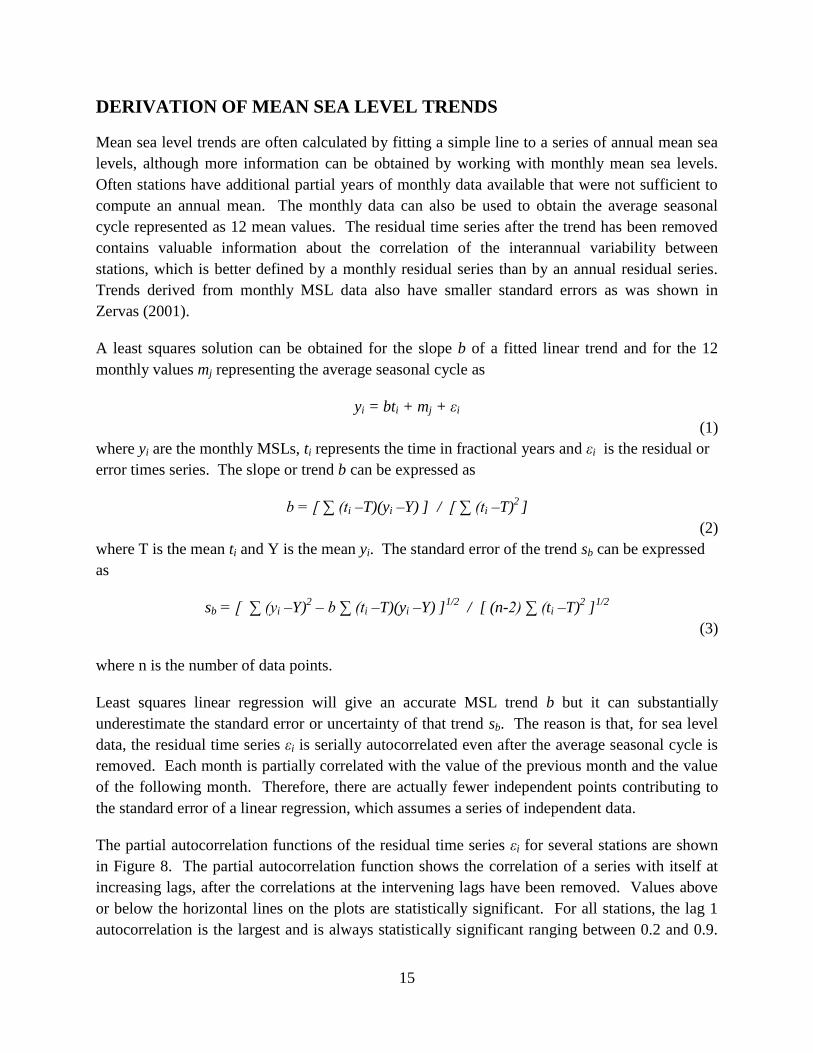
The partial autocorrelation functions of the residual time series εi for several stations are shown

in Figure 8. The partial autocorrelation function shows the correlation of a series with itself at

increasing lags, after the correlations at the intervening lags have been removed. Values above

or below the horizontal lines on the plots are statistically significant. For all stations, the lag 1

autocorrelation is the largest and is always statistically significant ranging between 0.2 and 0.9.

16

At many stations, none of the higher lags are statistically significant; at other stations, some

higher lags are marginally significant but less than the lag 1 autocorrelation.

Figure 8. Partial autocorrelation functions of residual time series versus lag in months. Values above or

below the horizontal lines are statistically significant.

Therefore, following Zervas (2001), the monthly MSL data yi are characterized as an autoregres-

sive process of order 1 as

yi = bti + mj + ρ1 (yi-1 – bti-1 – mj-1) + εi

(4)

where ρ1 is the lag 1 autoregressive coefficient representing the part of the time series predictable

from the previous month’s residual, and εi is the error representing the random unpredictable part

of the residual. ρ1 ranges between -1 and +1 with 0 meaning the next value is completely

17

unpredictable (i.e., the residual is a random time series) and +1 meaning that the best guess for

the next residual is the current residual.

Since an extra parameter ρ1 is being solved for with the same amount of data, the uncertainty of

the solution is greater. The amount that the standard error of the trend sb is increased when using

the autoregressive solution instead of the linear regression solution can be approximated by the

square root of the variance inflation factor (Storch and Zwiers 2001, Wilks 2006) as

sb(autoregression) / sb(linear regression) = [ (1 + ρ1) / (1 – ρ1) ]1/2

(5)

The effect of increasing serial correlation on the standard error is shown in Table 3. A larger

standard error results in wider error bars associated with the derived parameter. Therefore, for

example, if the lag 1 autoregressive coefficient is 0.6, the correct standard error should be 2

times the standard error that would be obtained by applying a simple linear regression.

For some of the stations, there was an apparent datum shift or a seismic offset in the time series.

For an apparent datum shift, the trend should be the same before and after the shift. For an

earthquake, there may be a detectable seismic offset and/or the trend has the possibility of being

different before and after the earthquake. It can be assumed that the average seasonal cycle does

not change as a result of these events.

To incorporate an unknown datum shift at a known time into the solution, the equation solved for

is

yi = bti + mj + dfi + ρ1 (yi-1 – bti-1 – mj-1 – dfi-1) + εi

(6)

where d is the magnitude of the datum shift and fi is a step function with a value of 1 before the

shift and 0 after the shift.

Table 3. Effect of serial correlation of time series residuals on standard errors

Autoregressive

Coefficient

Variance

Inflation Factor

Ratio of

Standard Errors

0 1.0 1.0

0.2 1.5 1.225

0.4 2.333 1.528

0.6 4.0 2.0

0.8 9.0 3.0

18

To incorporate an earthquake at a known time into the solution, the equation solved for is

yi = b1fiti + b2(1-fi)ti + mj + dfi + ρ1 (yi-1 – b1fi-1ti-1 – b2(1-fi-1)ti-1 – mj-1 – dfi-1) + εi

(7)

where d is the magnitude of the seismic offset, b1 is the trend before the earthquake, b2 is the

trend after the earthquake, and fi is a step function with a value of 1 before the offset and 0 after

the offset.

19

LINEAR MEAN SEA LEVEL TRENDS

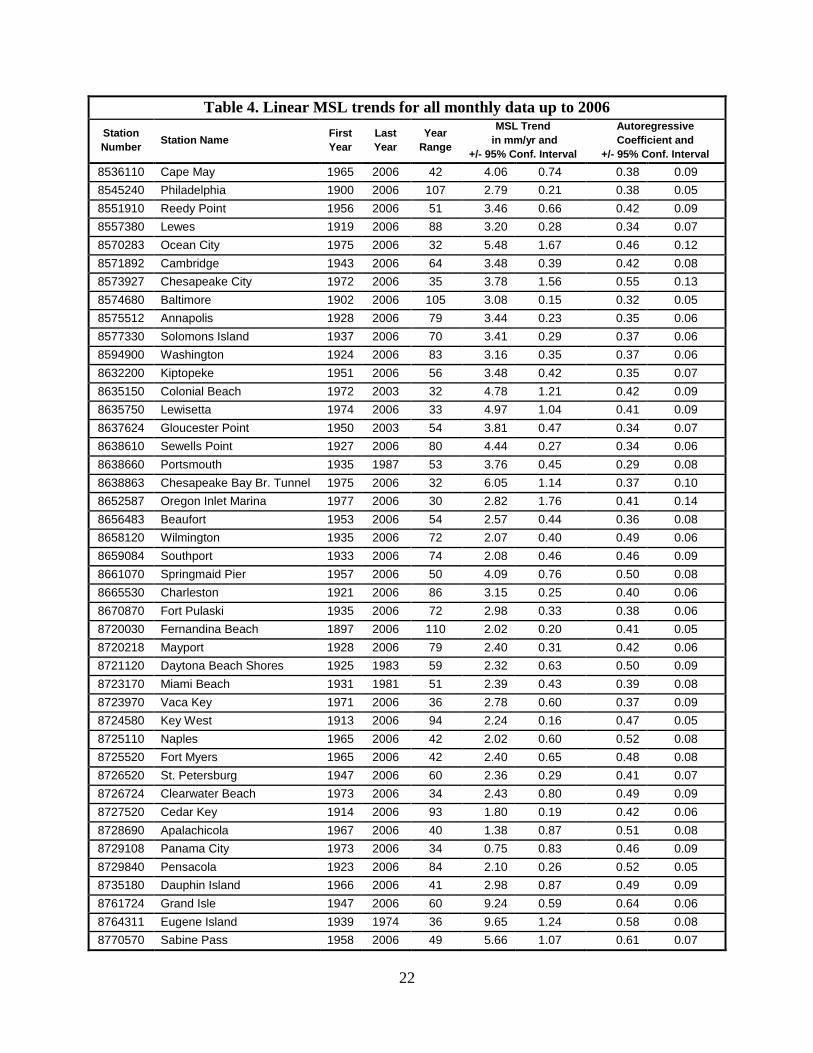
The 128 selected NWLON stations were analyzed using the methods described in the previous

section and the resulting MSL trends are listed in Table 4, which gives the first year and last year

of data, the year range, the linear trend with its 95% confidence interval, and the autoregressive

coefficient with its 95% confidence interval. The 95% confidence intervals are 1.96 times the

standard error above and below the derived value. The 95% confidence intervals are narrowest

for the stations with the longest year range of data. If a seismic offset and an associated change

in trend are included in the analysis, both pre-seismic and post-seismic trends are given in Table

4. Appendix II contains plots of the monthly MSLs after the average seasonal cycle has been

removed, the calculated trend line, and its 95% confidence interval. A 5-month running average

is also displayed to smooth out month-to-month variability and focus more attention on longer-

term anomalies. Solid vertical lines indicate the times of any nearby major earthquakes. Periods

of questionable data that appear to be offset are bracketed by dashed vertical lines.

The monthly MSL data plotted in Appendix II are relative to the MSL datum presently in effect.

For most stations, it is the MSL datum for the NTDE of 1983-2001. This is apparent in the plots,

as the calculated trends appear to cross zero around 1992, the middle year of the NTDE. For

stations where sea level has been rapidly rising or falling, CO-OPS has created special 5-year

MSL datums. For those station’s plots, the calculated trends cross zero near the middle of those

periods. The Galveston Pier 21, Galveston Pleasure Pier, Freeport, Anchorage, and Unalaska

MSL datums are for 1997-2001. The Grand Isle, Rockport, Juneau, Skagway, Yakutat, Seldovia,

Nikiski, and Kodiak Island MSL datums are for 2002-2006. Eugene Island has no recent data so

it is presented on its old 1960-1978 MSL datum. Guantanamo Bay has no established datum so

it is presented on its own arbitrary station datum.

The main difference between the trends in Table 4 and the trends in the previous report (Zervas

2001), is the reduction in the widths of the 95% confidence intervals achieved by using seven

additional years of data. Many of the shortest-period U.S. west coast stations have slightly lower

trends using data up to 2006 compared to trends using data up to 1999. The reason is that the

high water levels in 1997-1998 due to a strong El Niño event resulted in a small upward bias in

the previously calculated trends, although none of the differences are statistically significant at

the 95% confidence level. Only five stations have a new trend that is outside of the 95%

confidence intervals previously calculated in Zervas (2001). These stations are Springmaid Pier,

Freeport, Yakutat, Cordova, and Valdez and all have lower trends than in Zervas (2001).

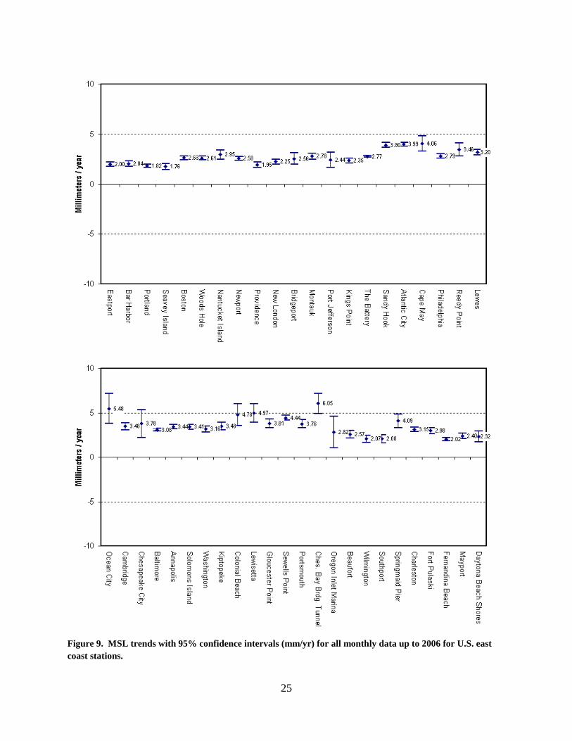
Most of the U.S. east coast stations that are compared in Figure 9 have been in operation for

many decades, making it possible to detect statistically significant differences in trends among

the stations. All of the trends are above the global 20th

century average of 1.7 mm/yr indicating

that some land subsidence is included in most of the trends. There are higher trends in the mid-

Atlantic coastal region from New Jersey to Virginia than in the regions to the north or to the

20

south. This pattern is often attributed to the ongoing collapse of the peripheral bulge that was

formed as a result of visco-elastic lithospheric compensation during the previous ice age, due to

the weight of the ice sheet (Douglas 1991, Davis and Mitrovica 1996). The highest east coast

trend is 6.05 mm/yr at the Chesapeake Bay Bridge Tunnel station which is located on a man-

made structure and therefore, its rate may not be representative of a wider area.

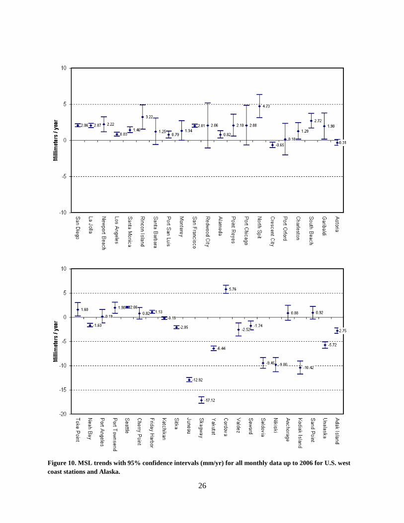
The MSL trends at the U.S. west coast and Alaska stations compared in Figure 10 are much

more spatially variable due to tectonic activity at plate boundaries. There are also more shorter-

period stations with correspondingly wider 95% confidence intervals. Most of the trends are

close to or below the global 20th

century rate of 1.7 mm/yr with the exceptions of Rincon Island,

North Spit, South Beach, and Cordova where some localized land subsidence is likely to be

occurring. Rapidly falling sea levels indicate substantial uplift at Juneau and Skagway due to

localized glacial melting, and at Seldovia, Nikiski, Kodiak Island, and Unalaska due to post-

seismic tectonic processes. Both processes may be occurring at Yakutat. Smaller rates of

vertical land uplift are apparent at various other locations in Alaska and in Washington, Oregon,

and California. The most negative MSL trend at any NWLON station is -17.12 mm/yr at

Skagway located at the upper end of a glacial fjord.

Most of the station trends for the tropical Pacific, Bermuda, the Gulf of Mexico, and the

Caribbean, compared in Figure 11, are reasonably close to the global 20th

century rate with the

exception of the stations in Louisiana and Texas where substantial subsidence is occurring. The

western part of the U.S. Gulf coast has been experiencing sediment loading, soil compaction, and

high rates of oil, gas, and groundwater extraction. The highest MSL trends are at Grand Isle and

Eugene Island in Louisiana. The trend at Hilo is somewhat higher than the trends at the other

Hawaiian stations perhaps from crustal subsidence due to active volcanic loading of the Pacific

plate. The negative trend at Guam is only for the period before the 1993 8.0-magnitude

earthquake when a 10-cm offset is apparent in the detided hourly water level record. Since 1993,

Guam has experienced a large positive MSL trend.

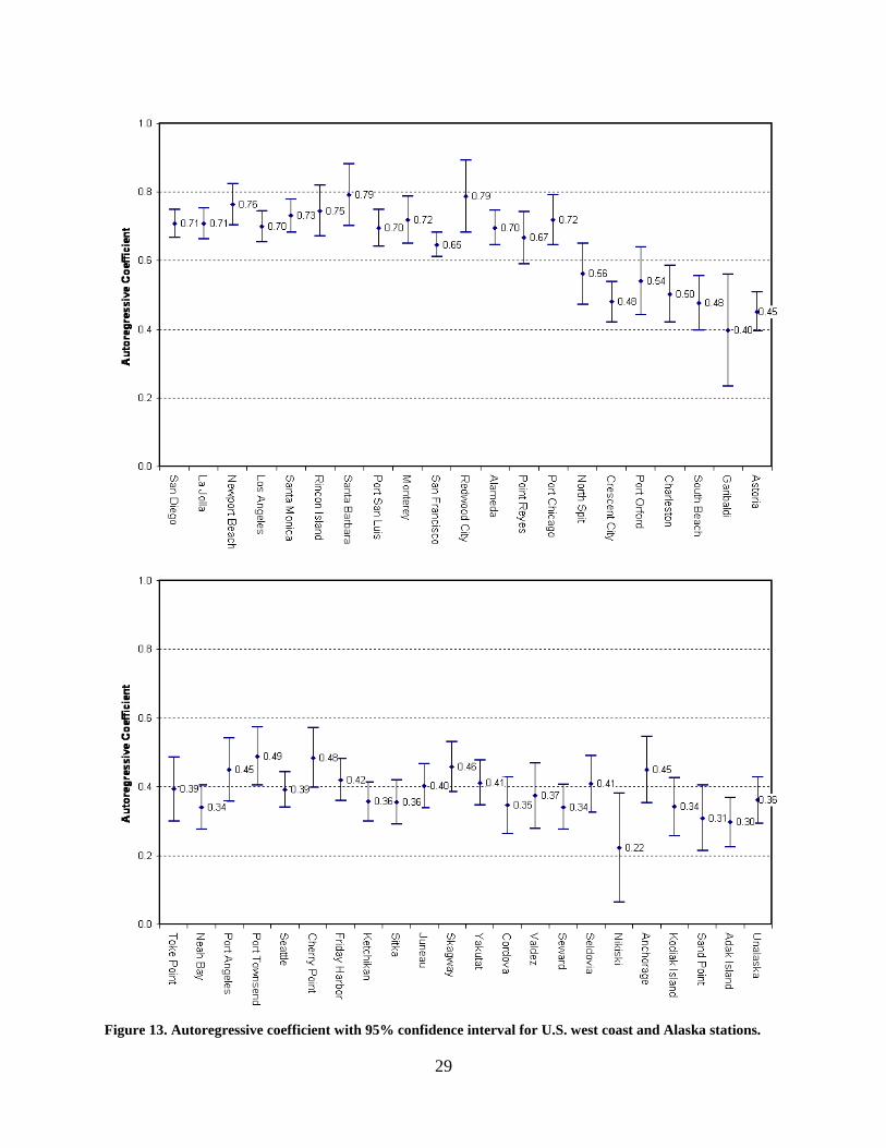
The autoregressive coefficients for all the stations are compared in Figures 12-14. The

autoregressive coefficient can range between -1 and +1 and indicates how predictable a monthly

MSL residual is from the previous month’s MSL residual. Values near +1 indicate that if one

month’s residual is positive, the next month’s residual is also highly likely to be positive; values

near -1 indicate that if one month’s residual is positive, the next month’s residual is highly likely

to be negative. The highest positive values are found at stations dominated by the El Niño

Southern Oscillation (ENSO) with very little month-to-month variability. The characteristic

effects of ENSO on Pacific Ocean water level variability will be discussed later in this report.

The autoregressive coefficients for U.S. east coast stations range between 0.3 and 0.5. For U.S.

west coast stations, autoregressive coefficients are near 0.7 at stations from San Diego to the San

Francisco Bay area which are dominated by the ENSO signal. They fall back to the 0.3-0.5

21

range for northern California, Oregon, Washington, and Alaska stations which also contain

ENSO forcing but have substantial month-to-month variability. Most of the Gulf coast stations

have autoregressive coefficients varying between 0.4 and 0.6 with values slightly increasing

from east to west. The Hawaiian and Caribbean autoregressive coefficients are clustered around

0.7, while Johnston Atoll, Midway Atoll, Wake Island, and Bermuda have smaller values near

0.5 due to greater month-to-month variability. The highest autoregressive coefficients, over 0.8,

are found at the west and south Pacific stations (Guam, Pago Pago, Kwajalein, and Chuuk) that

are dominated by the ENSO signal, as will be demonstrated later in this report.

Table 4. Linear MSL trends for all monthly data up to 2006

Station

Number Station Name

First

Year

Last

Year

Year

Range

MSL Trend

in mm/yr and

+/- 95% Conf. Interval

Autoregressive

Coefficient and

+/- 95% Conf. Interval

1611400 Nawiliwili 1955 2006 52 1.53 0.59 0.65 0.06

1612340 Honolulu 1905 2006 102 1.50 0.25 0.74 0.04

1612480 Mokuoloe 1957 2006 50 1.31 0.72 0.71 0.06

1615680 Kahului 1947 2006 60 2.32 0.53 0.75 0.05

1617760 Hilo 1927 2006 80 3.27 0.35 0.63 0.05

1619000 Johnston Atoll 1947 2003 57 0.75 0.56 0.43 0.07

1619910 Midway Atoll 1947 2006 60 0.70 0.54 0.57 0.06

1630000 Guam (Pre EQ) 1948 1993 46 -1.05 1.72 0.86 0.04

1630000 Guam (Post EQ) 1993 2006 14 8.58 8.93

1770000 Pago Pago 1948 2006 59 2.07 0.90 0.82 0.04

1820000 Kwajalein 1946 2006 61 1.43 0.81 0.84 0.04

1840000 Chuuk 1947 1995 49 0.60 1.78 0.85 0.05

1890000 Wake Island 1950 2006 57 1.91 0.59 0.47 0.07

2695540 Bermuda 1932 2006 75 2.04 0.47 0.45 0.06

8410140 Eastport 1929 2006 78 2.00 0.21 0.45 0.06

8413320 Bar Harbor 1947 2006 60 2.04 0.26 0.34 0.07

8418150 Portland 1912 2006 95 1.82 0.17 0.45 0.05

8419870 Seavey Island 1926 2001 76 1.76 0.30 0.37 0.07

8443970 Boston 1921 2006 86 2.63 0.18 0.39 0.06

8447930 Woods Hole 1932 2006 75 2.61 0.20 0.39 0.06

8449130 Nantucket Island 1965 2006 42 2.95 0.46 0.33 0.08

8452660 Newport 1930 2006 77 2.58 0.19 0.35 0.06

8454000 Providence 1938 2006 69 1.95 0.28 0.47 0.07

8461490 New London 1938 2006 69 2.25 0.25 0.39 0.06

8467150 Bridgeport 1964 2006 43 2.56 0.58 0.39 0.08

8510560 Montauk 1947 2006 60 2.78 0.32 0.35 0.07

8514560 Port Jefferson 1957 1992 36 2.44 0.76 0.39 0.09

8516945 Kings Point / Willets Point 1931 2006 76 2.35 0.24 0.32 0.06

8518750 The Battery 1856 2006 151 2.77 0.09 0.33 0.05

8531680 Sandy Hook 1932 2006 75 3.90 0.25 0.32 0.06

8534720 Atlantic City 1911 2006 96 3.99 0.18 0.30 0.06

22

Table 4. Linear MSL trends for all monthly data up to 2006

Station

Number Station Name

First

Year

Last

Year

Year

Range

MSL Trend

in mm/yr and

+/- 95% Conf. Interval

Autoregressive

Coefficient and

+/- 95% Conf. Interval

8536110 Cape May 1965 2006 42 4.06 0.74 0.38 0.09

8545240 Philadelphia 1900 2006 107 2.79 0.21 0.38 0.05

8551910 Reedy Point 1956 2006 51 3.46 0.66 0.42 0.09

8557380 Lewes 1919 2006 88 3.20 0.28 0.34 0.07

8570283 Ocean City 1975 2006 32 5.48 1.67 0.46 0.12

8571892 Cambridge 1943 2006 64 3.48 0.39 0.42 0.08

8573927 Chesapeake City 1972 2006 35 3.78 1.56 0.55 0.13

8574680 Baltimore 1902 2006 105 3.08 0.15 0.32 0.05

8575512 Annapolis 1928 2006 79 3.44 0.23 0.35 0.06

8577330 Solomons Island 1937 2006 70 3.41 0.29 0.37 0.06

8594900 Washington 1924 2006 83 3.16 0.35 0.37 0.06

8632200 Kiptopeke 1951 2006 56 3.48 0.42 0.35 0.07

8635150 Colonial Beach 1972 2003 32 4.78 1.21 0.42 0.09

8635750 Lewisetta 1974 2006 33 4.97 1.04 0.41 0.09

8637624 Gloucester Point 1950 2003 54 3.81 0.47 0.34 0.07

8638610 Sewells Point 1927 2006 80 4.44 0.27 0.34 0.06

8638660 Portsmouth 1935 1987 53 3.76 0.45 0.29 0.08

8638863 Chesapeake Bay Br. Tunnel 1975 2006 32 6.05 1.14 0.37 0.10

8652587 Oregon Inlet Marina 1977 2006 30 2.82 1.76 0.41 0.14

8656483 Beaufort 1953 2006 54 2.57 0.44 0.36 0.08

8658120 Wilmington 1935 2006 72 2.07 0.40 0.49 0.06

8659084 Southport 1933 2006 74 2.08 0.46 0.46 0.09

8661070 Springmaid Pier 1957 2006 50 4.09 0.76 0.50 0.08

8665530 Charleston 1921 2006 86 3.15 0.25 0.40 0.06

8670870 Fort Pulaski 1935 2006 72 2.98 0.33 0.38 0.06

8720030 Fernandina Beach 1897 2006 110 2.02 0.20 0.41 0.05

8720218 Mayport 1928 2006 79 2.40 0.31 0.42 0.06

8721120 Daytona Beach Shores 1925 1983 59 2.32 0.63 0.50 0.09

8723170 Miami Beach 1931 1981 51 2.39 0.43 0.39 0.08

8723970 Vaca Key 1971 2006 36 2.78 0.60 0.37 0.09

8724580 Key West 1913 2006 94 2.24 0.16 0.47 0.05

8725110 Naples 1965 2006 42 2.02 0.60 0.52 0.08

8725520 Fort Myers 1965 2006 42 2.40 0.65 0.48 0.08

8726520 St. Petersburg 1947 2006 60 2.36 0.29 0.41 0.07

8726724 Clearwater Beach 1973 2006 34 2.43 0.80 0.49 0.09

8727520 Cedar Key 1914 2006 93 1.80 0.19 0.42 0.06

8728690 Apalachicola 1967 2006 40 1.38 0.87 0.51 0.08

8729108 Panama City 1973 2006 34 0.75 0.83 0.46 0.09

8729840 Pensacola 1923 2006 84 2.10 0.26 0.52 0.05

8735180 Dauphin Island 1966 2006 41 2.98 0.87 0.49 0.09

8761724 Grand Isle 1947 2006 60 9.24 0.59 0.64 0.06

8764311 Eugene Island 1939 1974 36 9.65 1.24 0.58 0.08

8770570 Sabine Pass 1958 2006 49 5.66 1.07 0.61 0.07

23

Table 4. Linear MSL trends for all monthly data up to 2006

Station

Number Station Name

First

Year

Last

Year

Year

Range

MSL Trend

in mm/yr and

+/- 95% Conf. Interval

Autoregressive

Coefficient and

+/- 95% Conf. Interval

8771450 Galveston Pier 21 1908 2006 99 6.39 0.28 0.53 0.05

8771510 Galveston Pleasure Pier 1957 2006 50 6.84 0.81 0.54 0.07

8772440 Freeport 1954 2006 53 4.35 1.12 0.50 0.07

8774770 Rockport 1948 2006 59 5.16 0.67 0.54 0.07

8778490 Port Mansfield 1963 2006 44 1.93 0.97 0.54 0.08

8779751 Padre Island 1958 2006 49 3.48 0.75 0.55 0.08

8779770 Port Isabel 1944 2006 63 3.64 0.44 0.50 0.06

9410170 San Diego 1906 2006 101 2.06 0.20 0.71 0.04

9410230 La Jolla 1924 2006 83 2.07 0.29 0.71 0.05

9410580 Newport Beach 1955 1993 39 2.22 1.04 0.76 0.06

9410660 Los Angeles 1923 2006 84 0.83 0.27 0.70 0.04

9410840 Santa Monica 1933 2006 74 1.46 0.40 0.73 0.05

9411270 Rincon Island 1962 1990 29 3.22 1.66 0.75 0.07

9411340 Santa Barbara 1973 2006 34 1.25 1.82 0.79 0.09

9412110 Port San Luis 1945 2006 62 0.79 0.48 0.70 0.05

9413450 Monterey 1973 2006 34 1.34 1.35 0.72 0.07

9414290 San Francisco 1854 1897 44 2.05 0.85 0.65 0.04

9414290 San Francisco 1897 2006 110 2.01 0.21

9414523 Redwood City 1974 2006 33 2.06 3.12 0.79 0.11

9414750 Alameda 1939 2006 68 0.82 0.51 0.70 0.05

9415020 Point Reyes 1975 2006 32 2.10 1.52 0.67 0.08

9415144 Port Chicago 1976 2006 31 2.08 2.74 0.72 0.07

9418767 North Spit 1977 2006 30 4.73 1.58 0.56 0.09

9419750 Crescent City 1933 2006 74 -0.65 0.36 0.48 0.06

9431647 Port Orford 1977 2006 30 0.18 2.18 0.54 0.10

9432780 Charleston 1970 2006 37 1.29 1.15 0.50 0.08

9435380 South Beach 1967 2006 40 2.72 1.03 0.48 0.08

9437540 Garibaldi 1970 2006 37 1.98 1.82 0.40 0.16

9439040 Astoria 1925 2006 82 -0.31 0.40 0.45 0.06

9440910 Toke Point 1973 2006 34 1.60 1.38 0.39 0.09

9443090 Neah Bay 1934 2006 73 -1.63 0.36 0.34 0.06

9444090 Port Angeles 1975 2006 32 0.19 1.39 0.45 0.09

9444900 Port Townsend 1972 2006 35 1.98 1.15 0.49 0.08

9447130 Seattle 1898 2006 109 2.06 0.17 0.39 0.05

9449424 Cherry Point 1973 2006 34 0.82 1.20 0.48 0.09

9449880 Friday Harbor 1934 2006 73 1.13 0.33 0.42 0.06

9450460 Ketchikan 1919 2006 88 -0.19 0.27 0.36 0.06

9451600 Sitka 1924 2006 83 -2.05 0.32 0.36 0.06

9452210 Juneau 1936 2006 71 -12.92 0.43 0.40 0.06

9452400 Skagway 1944 2006 63 -17.12 0.65 0.46 0.07

9453220 Yakutat 1940 2006 67 -6.44 0.47 0.41 0.06

9453220 Yakutat (Pre EQ) 1940 1979 40 -4.81 0.89 0.32 0.07

9453220 Yakutat (Post EQ) 1979 2006 28 -11.53 1.46

24

Table 4. Linear MSL trends for all monthly data up to 2006

Station

Number Station Name

First

Year

Last

Year

Year

Range

MSL Trend

in mm/yr and

+/- 95% Conf. Interval

Autoregressive

Coefficient and

+/- 95% Conf. Interval

9454050 Cordova (Pre EQ) 1949 1961 13 5.01 10.92 0.35 0.08

9454050 Cordova (Post EQ) 1964 2006 43 5.76 0.87

9454240 Valdez 1973 2006 34 -2.52 1.36 0.37 0.10

9455090 Seward (Pre EQ) 1925 1964 40 -0.11 1.08 0.34 0.06

9455090 Seward (Post EQ) 1964 2006 43 -1.74 0.91

9455500 Seldovia 1964 2006 43 -9.45 1.10 0.41 0.08

9455760 Nikiski 1973 2006 34 -9.80 1.50 0.22 0.16

9455920 Anchorage 1972 2006 35 0.88 1.54 0.45 0.10

9457292 Kodiak Island (Pre EQ) 1949 1964 16 1.19 3.70 0.34 0.09

9457292 Kodiak Island (Post EQ) 1975 2006 32 -10.42 1.33

9459450 Sand Point 1972 2006 35 0.92 1.32 0.31 0.10

9461380 Adak Island (Pre EQ) 1943 1957 15 2.45 3.61 0.30 0.07

9461380 Adak Island (Post EQ) 1957 2006 50 -2.75 0.54

9462620 Unalaska (Pre EQ) 1934 1957 24 -0.57 2.16 0.36 0.07

9462620 Unalaska (Post EQ) 1957 2006 50 -5.72 0.67

9731158 Guantanamo Bay 1937 1971 35 1.64 0.80 0.65 0.08

9751401 Lime Tree Bay 1977 2006 30 1.74 1.20 0.65 0.09

9751639 Charlotte Amalie 1975 2006 32 1.20 0.96 0.72 0.07

9755371 San Juan 1962 2006 45 1.65 0.52 0.66 0.07

9759110 Magueyes Island 1955 2006 52 1.35 0.37 0.68 0.06

25

Figure 9. MSL trends with 95% confidence intervals (mm/yr) for all monthly data up to 2006 for U.S. east

coast stations.

26

Figure 10. MSL trends with 95% confidence intervals (mm/yr) for all monthly data up to 2006 for U.S. west

coast stations and Alaska.

27

Figure 11. MSL trends and 95% confidence intervals (mm/yr) for all monthly data up to 2006 for Gulf of

Mexico, tropical Pacific, Bermuda, and Caribbean stations.

28

Figure 12. Autoregressive coefficient with 95% confidence interval for U.S. east coast stations.

29

Figure 13. Autoregressive coefficient with 95% confidence interval for U.S. west coast and Alaska stations.

30

Figure 14. Autoregressive coefficient with 95% confidence interval for Gulf of Mexico, tropical Pacific,

Bermuda, and Caribbean stations.

31

At six of the NWLON stations, there was clear evidence of a seismic offset and, for these

stations, an offset and a change in trend are included in the analyses. These events are the August

1993 earthquake affecting Guam, the March 1964 earthquake affecting Cordova, Seward, and

Kodiak Island, and the March 1957 earthquake affecting Unalaska and Adak Island. For Guam,

the high post-seismic trend of 8.58 +/- 8.93 mm/yr is based on only 14 years of data and,

therefore, has a large uncertainty. Satellite altimetry measurements since 1993 show

comparatively high sea level trends in the western Pacific region (Cazenave and Nerem 2004),

which suggests that the rate at Guam may be due to rapid absolute sea level rise rather than rapid

post-seismic land subsidence. For Cordova, Kodiak Island, Unalaska, and Adak Island, the pre-

seismic trends are based on only 13 to 24 years of data and therefore are highly uncertain. None

of these trends are statistically different from zero at the 95% confidence level. The pre-seismic

trend at Seward is based on 40 years of data and is therefore better determined, but it is also not

statistically different from zero. All of the post-seismic trends for the Alaskan stations are based

on 32 to 50 years of data and are statistically different from zero.

The record at the Yakutat station appears to be a special case. When a single line is fitted to the

entire time series, a trend of -6.44 mm/yr is obtained. Examination of the residual time series

and comparisons with residuals at nearby stations strongly suggest the possibility of nonlinearity

at Yakutat. One possible cause is increasing glacial melting in the region around Yakutat,

leading to increasing elastic rebound of the lithosphere and more rapidly falling sea levels.

Another possible cause is regional tectonic activity. There were four major earthquakes in the

region in July 1958, February 1979, November 1987, and March 1988, and it is possible that

offsets or changes in trends may be associated with one or more of these events. Yakutat is at

the border between the seismic zones of the 1958 and 1979 earthquakes. It is possible that there

was a steeper trend before the 1958 earthquake, a flatter trend between 1958 and either the 1979

or the 1987-1988 events, and then a steeper trend up to the present.

In order to avoid over-fitting the Yakutat time series with a series of short, highly uncertain

trends, only one alternative is presented to fitting the entire series with a single line. One offset

and a change in trend are modeled at the time of the February 1979 earthquake. The time series

further west at the Cordova and Valdez stations also suggest a possibility of a change in trend at

that time or at the time of the 1987-1988 earthquakes. When two trends are modeled at Yakutat,

the pre-1979 trend is -4.81 mm/yr and the post-1979 trend is -11.53 mm/yr (Figure 15).

32

a)

b)

Figure 15. Monthly MSL data for Yakutat after removal of the average seasonal cycle. Calculated trends are

shown with 95% confidence intervals. Possible MSL trends for Yakutat are a) a single trend of -6.44 +/- 0.47

mm/yr or b) a February 1979 offset and change in trend from -4.81 +/- 0.89 mm/yr to -11.53 +/- 1.46 mm/yr.

In the previous report (Zervas 2001), comparisons of the Freeport time series with nearby

stations showed that there may have been an apparent datum shift on January 1972. Further

examination of the station differences, indicates that there could have been either an

instantaneous shift or a short period of extremely rapid subsidence in 1969-1971. There has been

measureable subsidence in the Freeport area due to groundwater withdrawal (Sandeen and

Wesselman 1973). The series at Freeport is again modeled with an offset at January 1972 and

no associated change in trend (Figure 16). The resulting trend is 4.35 mm/yr and the resulting

offset is 0.190 m.

33

Figure 16. Monthly MSL data for Freeport after removal of the average seasonal cycle. The trend of 4.35 +/-

1.12 mm/yr was calculated with an apparent datum shift of 0.190 m on January 1972 and is shown with its

95% confidence interval.

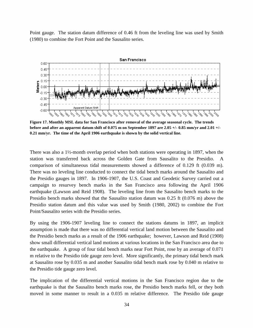
In the previous report (Zervas 2001), the long continuous time series for San Francisco was

initially fitted with a single trend; however, it seemed more likely that there was some non-

linearity in the time series, with a greater trend discernable in the 20th

century than in the 19th

century and apparently falling sea levels in the 50-year period centered around 1900. The station

is only 8 km from the San Andreas Fault which slipped in a major earthquake in April 1906.

Although there was no discernable offset at the time of the earthquake (Lawson and Reid 1908),

the series was fitted with a lower pre-seismic and a higher post-seismic trend implying a tectonic

cause for the change in trend (Zervas 2001).

Further investigation of the residual time series has shown that there was a discernable offset in

1897. The entire San Francisco series (Smith 1980, Smith 2002) had been put together by

combining data collected from three locations at Fort Point (1854-1877), Sausalito (1877-1897),

and the Presidio (since 1897). The timing of the apparent offset coincided with the time when

the station was moved back across the Golden Gate from Sausalito to the Presidio, which raises a

question about the accuracy of the connection between the two series. In this report, the series is

modeled with an apparent datum shift in September 1897 and separate trends before and after

that date, instead of with a seismic offset in April 1906. The trends before and after the apparent

datum shift are nearly identical (Figure 17).

Since the timing of the apparent offset coincided with the time when the station was moved

across the Golden Gate, the method used to link the three series together was re-examined. At

each location, measurements were recorded on an arbitrary tide gauge zero level known as the

station datum. There was a 9-month overlap period in 1877 while the station was first

transferred from Fort Point to Sausalito. Six months of simultaneous tidal measurements showed

a difference of 0.42 ft (0.128 m). A leveling line across the Golden Gate in 1877 showed that the

station datum of the Sausalito gauge was 0.46 ft (0.140 m) above the station datum of the Fort

34

Point gauge. The station datum difference of 0.46 ft from the leveling line was used by Smith

(1980) to combine the Fort Point and the Sausalito series.

Figure 17. Monthly MSL data for San Francisco after removal of the average seasonal cycle. The trends

before and after an apparent datum shift of 0.075 m on September 1897 are 2.05 +/- 0.85 mm/yr and 2.01 +/-

0.21 mm/yr. The time of the April 1906 earthquake is shown by the solid vertical line.

There was also a 1½-month overlap period when both stations were operating in 1897, when the

station was transferred back across the Golden Gate from Sausalito to the Presidio. A

comparison of simultaneous tidal measurements showed a difference of 0.129 ft (0.039 m).

There was no leveling line conducted to connect the tidal bench marks around the Sausalito and

the Presidio gauges in 1897. In 1906-1907, the U.S. Coast and Geodetic Survey carried out a

campaign to resurvey bench marks in the San Francisco area following the April 1906

earthquake (Lawson and Reid 1908). The leveling line from the Sausalito bench marks to the

Presidio bench marks showed that the Sausalito station datum was 0.25 ft (0.076 m) above the

Presidio station datum and this value was used by Smith (1980, 2002) to combine the Fort

Point/Sausalito series with the Presidio series.

By using the 1906-1907 leveling line to connect the stations datums in 1897, an implicit

assumption is made that there was no differential vertical land motion between the Sausalito and

the Presidio bench marks as a result of the 1906 earthquake; however, Lawson and Reid (1908)

show small differential vertical land motions at various locations in the San Francisco area due to

the earthquake. A group of four tidal bench marks near Fort Point, rose by an average of 0.071

m relative to the Presidio tide gauge zero level. More significantly, the primary tidal bench mark

at Sausalito rose by 0.035 m and another Sausalito tidal bench mark rose by 0.040 m relative to

the Presidio tide gauge zero level.

The implication of the differential vertical motions in the San Francisco region due to the

earthquake is that the Sausalito bench marks rose, the Presidio bench marks fell, or they both

moved in some manner to result in a 0.035 m relative difference. The Presidio tide gauge

35

recorded water levels before, during, and after the earthquake without a break and actually

recorded a small negative tsunami immediately after the earthquake; yet when the time series for

1906 is detided, no seismic offset can be discerned. Lawson and Reid (1908) also examined the

Presidio monthly mean sea levels from 1897 to 1907 and could find no evidence of a seismic

offset, although an offset as small as 0.035 m would be difficult to observe in the water level

time series given the non-tidal oceanographic variability.

Therefore, the station datum difference of 0.076 m used by Smith (1980) to combine the Fort

Point/Sausalito series with the Presidio series may include a seismic offset, which is introduced

into the combined series in 1897 by using a post-seismic leveling line to make a pre-seismic

connection. If the 0.035 m seismic movement of the Sausalito primary bench mark relative to

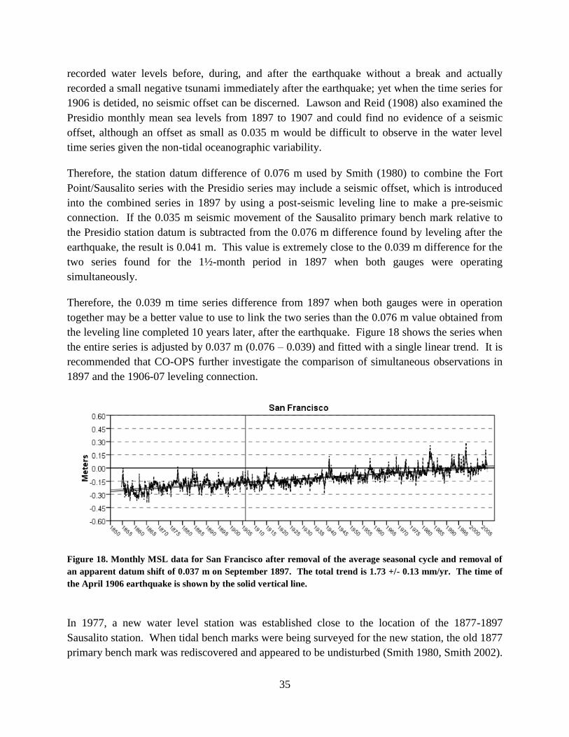
the Presidio station datum is subtracted from the 0.076 m difference found by leveling after the

earthquake, the result is 0.041 m. This value is extremely close to the 0.039 m difference for the

two series found for the 1½-month period in 1897 when both gauges were operating

simultaneously.

Therefore, the 0.039 m time series difference from 1897 when both gauges were in operation

together may be a better value to use to link the two series than the 0.076 m value obtained from

the leveling line completed 10 years later, after the earthquake. Figure 18 shows the series when

the entire series is adjusted by 0.037 m (0.076 – 0.039) and fitted with a single linear trend. It is

recommended that CO-OPS further investigate the comparison of simultaneous observations in

1897 and the 1906-07 leveling connection.

Figure 18. Monthly MSL data for San Francisco after removal of the average seasonal cycle and removal of

an apparent datum shift of 0.037 m on September 1897. The total trend is 1.73 +/- 0.13 mm/yr. The time of

the April 1906 earthquake is shown by the solid vertical line.

In 1977, a new water level station was established close to the location of the 1877-1897

Sausalito station. When tidal bench marks were being surveyed for the new station, the old 1877

primary bench mark was rediscovered and appeared to be undisturbed (Smith 1980, Smith 2002).

36

Data were collected for 2½ years until 1979 on a new station datum which was 2.72 ft (0.829 m)

above the old Sausalito station datum. Using this information, the 1877-1897 data can be

adjusted to the new station datum and a linear trend of 0.96 mm/yr is derived (Figure 19).

Figure 19. Monthly MSL data for Sausalito after removal of the average seasonal cycle. The total trend is

0.96 +/- 0.54 mm/yr. The time of the April 1906 earthquake is shown by the solid vertical line.

Fitting a single trend to the Sausalito data ignores the possibility of any seismic offset in 1906,

but it is not possible to reasonably model the magnitude of an offset without any data

immediately before and after the offset. If there was no seismic offset or even with a small offset

of only 0.035 m, the trend is significantly lower than the 2.01 +/- 0.21 mm/yr trend at the

Presidio since 1897. This is certainly possible due to differential tectonic uplift in between the

multiple fault lines throughout the San Francisco Bay region. The station at Alameda about 15

km to the east was established in 1939, and has a trend of only 0.82 +/- 0.51 mm/yr, which is a

statistically significant difference relative to the San Francisco trend.

37

AVERAGE SEASONAL MEAN SEA LEVEL CYCLE

By using monthly MSL data to derive the linear trends discussed in the previous section, twelve

calendar monthly means are also obtained that define the average seasonal cycle. These monthly

values for each station are listed in Table B in Appendix III and are also plotted in Appendix III

with their 95% confidence intervals. The average seasonal cycle can be considered as the

regular, repeatable variation over the course of a year which becomes more precisely defined as

more years of data are accumulated.

The average seasonal cycles for coastal water levels are caused by a combination of the effects of

the average seasonal cycles of air pressure, wind, water temperature, salinity, ocean currents, and

river discharge. For many stations, the average seasonal cycle is mainly driven by the steric

effect, which is the change in the volume of seawater caused by changes in water density due to

temperature and salinity variations. Water levels tend to be highest in late summer/early fall at

the end of the heating season and lowest in the late winter/early spring at the end of the cooling

season.

Pago Pago and Eastport have essentially no seasonal cycle with no monthly values significantly

higher or lower than any other month. The largest seasonal cycles are at Fernandina Beach and

Toke Point with a range over 0.3 meters. Philadelphia has continuously high water levels from

April to September, caused by a combination of higher river flow in the spring and the steric

effect in the summer.

The Atlantic coast stations from South Carolina to northern Florida and the Gulf of Mexico

stations from Alabama to Texas have a double-peaked average seasonal cycle. They generally

rise from their lowest winter level in January to a secondary peak in May or June, fall to a

secondary low in July, before rising to their highest level in September or October. On the

Atlantic coast, this modification of the usual steric seasonal cycle has been attributed to the

dynamic effect of seasonal variations in the speed of the Gulf Stream (Noble and Gelfenbaum

1992, Blaha 1984). The mass transport of the Florida Current, which connects the Loop Current

in the Gulf of Mexico to the Gulf Stream in the Atlantic, is lowest in January and peaks in July

(Baringer and Larsen 2001), although it is highly variable from year to year.

The dynamic effect of the California Current has a strong influence on the average seasonal

cycles of stations in northern California, Oregon, and Washington which have their lowest levels

in spring and summer when the wind-driven southward current is usually strongest, causing the

upwelling of cold water along the coast. The seasonal cycles for Alaskan stations also reach

their lowest levels in spring or early summer, influenced by variation in the strength of the

northwest-flowing Alaska Current.

Traditional tide prediction is accomplished by summing a series of sinusoidal curves at a limited

number of frequencies known as the tidal harmonic constituents (Schureman 1958). The

38

constituents are primarily diurnal and semidiurnal, but they also include the solar annual

constituent Sa and the solar semiannual constituent Ssa. Although there is a small astronomical

tide-producing force at these frequencies, most of the water level variation found by harmonic

analysis at these frequencies is the climate-driven average seasonal cycle. As a result, Sa and

Ssa are sometimes referred to as meteorological constituents (Center for Operational

Oceanographic Products and Services 1999). It is important to include them in tide predictions;

without them, observations will appear to be noticeably higher or lower than the predicted tide at

various times of the year.

CO-OPS, which is charged with making the official tide predictions for the United States,

derives a unique set of tidal constituents classified as “accepted” for each station. For long-term

stations, the tidal constituents from as many as five 1-year harmonic analyses are usually

averaged to obtain the diurnal and semidiurnal tidal constituents; however, the Sa and the Ssa

constituents are usually derived by averaging the results of as many as 19 years (a tidal epoch) of

1-year harmonic analyses. If they are generally consistent in amplitude and phase for each year,

they are accepted and included in the set of constituents used for tide prediction. If they are not

very consistent from year to year, they are not included in the accepted set of tide constituents for

that station. For some shorter-term stations such as Chesapeake City and Redwood City, the Sa

and Ssa constituents of a nearby longer-term station have been adopted. The accepted tidal

constituents can be found on the CO-OPS website

(http://tidesandcurrents.noaa.gov/station_retrieve.shtml?type=Harmonic+Constituents)

For this report, the twelve monthly values of the average seasonal cycles in Table B of Appendix

III have been used to derive the amplitudes and phases of the Sa and Ssa tidal constituents using

the CO-OPS tidal harmonic analysis program (Zervas 1999). The results are listed in Table C of

Appendix IV. The values of the accepted tidal constituents that CO-OPS uses to make the

official tide predictions are also listed for comparison. The amplitudes and phases of Sa and Ssa

are also compared by region in Figures 20 to 25. The values derived for this report are indicated

by the filled symbols while the accepted CO-OPS tide constituents are indicated by the unfilled

symbols. If CO-OPS has no accepted set of constituents, there are blank spaces in Table C and

no symbols are plotted on the figures. If CO-OPS has a set of accepted constituents that doesn’t

include Sa or Ssa, there are zeros in Table C and the unfilled symbols on the figures are plotted

at zero.

It is apparent from Figures 20 to 25 that for most stations the CO-OPS accepted values for Sa

and Ssa closely correspond with the values derived from the average seasonal cycle which is

based on the entire record at each station instead of 19 years or fewer. It is also apparent that the

constituents vary smoothly in amplitude and phase from one station to the next along each

coastline. The Sa amplitude is usually larger than the Ssa amplitude. The exceptions are at

Eastport, Port Chicago, and at all the stations in Texas where Ssa is stronger than Sa.

39

At some stations, the weaker Ssa constituent has been zeroed out while only the stronger Sa

constituent is used in CO-OPS tide predictions. Comparisons with derived values at neighboring

stations indicate that the Ssa amplitudes and phases are highly consistent along a coastline and

Ssa values could be used in the predictions. At Wilmington and Port Chicago, the Sa constituent

is zeroed out while only the Ssa constituent is used in the official tide predictions.

At Bar Harbor, Ocean City, Southport, Eugene Island, Garibaldi, Mokuoloe, Guam, Pago Pago,

and Kwajalein, both Sa and Ssa are set to zero in the accepted set of constituents, so no seasonal

cycles are used in the CO-OPS tide predictions. Guam, Pago Pago, and Kwajalein are strongly

influenced by the interannual ENSO forcing. Therefore, any Sa or Ssa obtained by harmonic

analysis of a year affected by a strong El Niño or La Niña event will be very different from those

obtained by harmonic analysis of ENSO-neutral years. However, tide predictions without Sa or

Ssa will not reflect the seasonal cycle even in ENSO-neutral years.

Although at most stations the accepted constituents compare very well with the constituents

derived from the average seasonal cycles, there are some differences. At Montauk and

Philadelphia, the accepted Sa and Ssa amplitudes appear to be twice the amplitudes derived from

the average seasonal cycle. At Anchorage, the accepted Ssa amplitude is greater than the Sa

amplitude which doesn’t correspond with its average seasonal cycle or with the Ssa amplitude at

any of the other Alaskan stations. At Newport and Fernandina Beach, there appears to be a

problem with the accepted phase of Sa. It is recommended that CO-OPS investigate these

discrepancies and update the constituents as necessary.

40

0

0.02

0.04

0.06

0.08

0.1

0.12

0.14

0.16

0.18

Eastp

ort

Bar H

arb

or

Portla

nd

Seavey Is

land

Bosto

n

Woods H

ole

Nantu

cket Is

land

New

port

Pro

vid

ence

New

London

Brid

geport

Monta

uk

Port J

effe

rson

Kin

gs P

oin

t

The B

atte

ry

Sandy H

ook

Atla

ntic

City

Cape M

ay

Phila

delp

hia

Reedy P

oin

t

Lew

es

Mete

rs

Sa Derived

Ssa Derived

Sa Accepted

Ssa Accepted

0

30

60

90

120

150

180

210

240

270

300

330

360

Ea

stp

ort

Ba

r Ha

rbo

r

Po

rtland

Se

ave

y Is

land

Bo

sto

n

Wo

ods H

ole

Na

ntu

cket Is

land

Ne

wp

ort

Pro

vid

en

ce

Ne

w L

on

do

n

Brid

ge

po

rt

Mo

nta

uk

Po

rt Je

ffers

on

Kin

gs P

oin

t

The

Ba

ttery

Sa

nd

y H

oo

k

Atla

ntic

City

Ca

pe

Ma

y

Ph

ilade

lphia

Re

ed

y P

oin

t

Lew

es

Deg

rees

Sa Derived

Ssa Derived

Sa Accepted

Ssa Accepted

Figure 20. Comparison of derived and accepted long-term tidal constituent amplitudes (top) and phases

(bottom) for northern U.S. east coast stations.

41

0

0.02

0.04

0.06

0.08

0.1

0.12

0.14

0.16

0.18

Ocean C

ity

Cam

brid

ge

Chesapeake C

ity

Baltim

ore

Annapolis

Solo

mons Is

land

Washin

gto

n

Colo

nia

l Beach

Lew

isetta

Kip

topeke

Glo

uceste

r Poin

t

Sew

ells

Poin

t

Ports

mouth

Ches B

ay B

ridge T

unnel

Ore

gon In

let M

arin

a

Beaufo

rt

Wilm

ingto

n

South

port

Sprin

gm

aid

Pie

r

Charle

sto

n

Fort P

ula

ski

Fern

andin

a B

each

Mayport

Dayto

na B

each S

hore

s

Mete

rs

Sa Derived

Ssa Derived

Sa Accepted

Ssa Accepted

0

30

60

90

120

150

180

210

240

270

300

330

360

Oce

an

City

Ca

mb

ridge

Ch

esa

pe

ake

City

Ba

ltimo

re

An

na

po

lis

So

lom

on

s Is

land

Wa

sh

ingto

n

Co

lonia

l Be

ach

Lew

ise

tta

Kip

top

eke

Glo

uce

ste

r Po

int

Se

we

lls P

oin

t

Po

rtsm

outh

Ch

es B

ay B

ridg

e T

un

ne

l

Ore

go

n In

let M

arin

a

Be

au

fort

Wilm

ingto

n

So

uth

po

rt

Sp

ring

ma

id P

ier

Ch

arle

sto

n

Fort P

ula

ski

Fern

an

din

a B

each

Ma

ypo

rt

Da

yto

na

Bea

ch S

hore

s

Deg

rees

Sa Derived

Ssa Derived

Sa Accepted

Ssa Accepted

Figure 21. Comparison of derived and accepted long-term tidal constituent amplitudes (top) and phases

(bottom) for southern U.S. east coast stations.

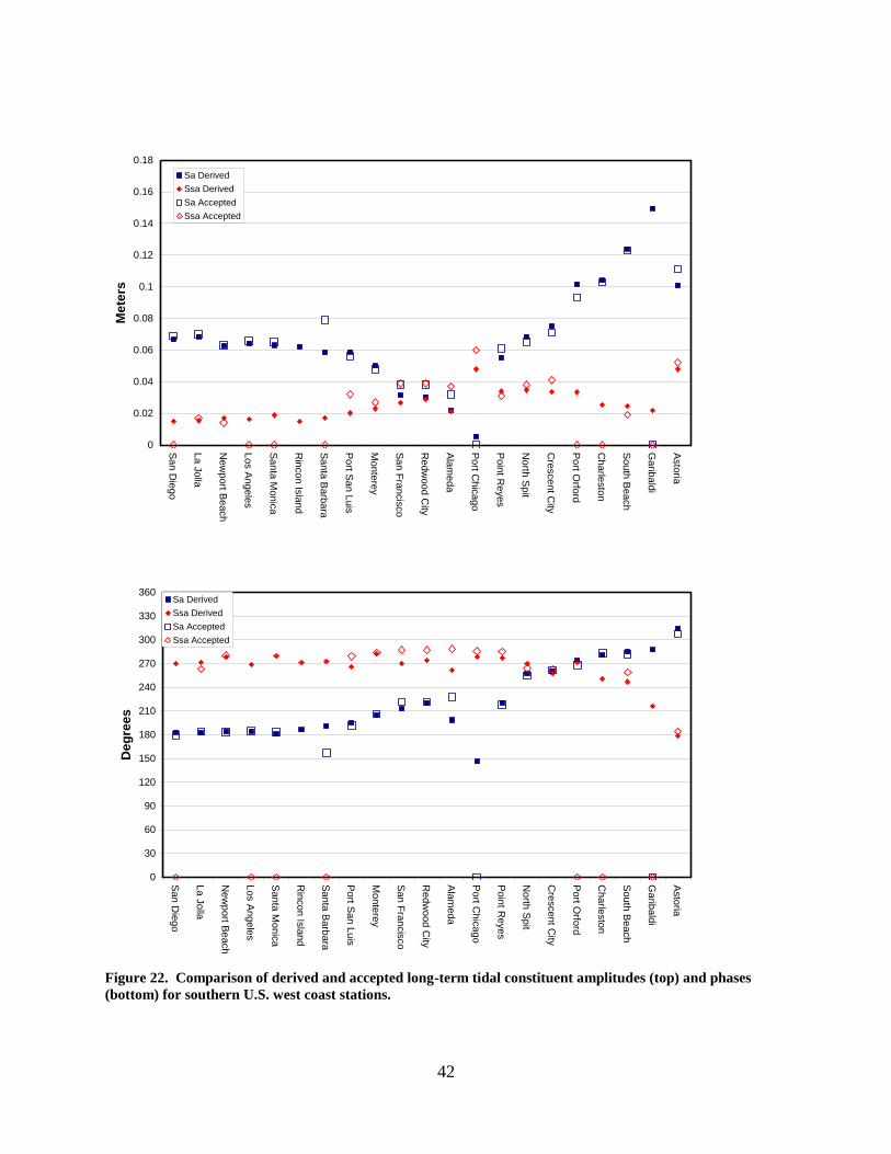
42

0

0.02

0.04

0.06

0.08

0.1

0.12

0.14

0.16

0.18

San D

iego

La J

olla

New

port B

each

Los A

ngele

s

Santa

Monic

a

Rin

con Is

land

Santa

Barb

ara

Port S

an L

uis

Monte

rey

San F

rancis

co

Redw

ood C

ity

Ala

meda

Port C

hic

ago

Poin

t Reyes

North

Spit

Cre

scent C

ity

Port O

rford

Charle

sto

n

South

Beach

Garib

ald

i

Asto

ria

Mete

rs

Sa Derived

Ssa Derived

Sa Accepted

Ssa Accepted

0

30

60

90

120

150

180

210

240

270

300

330

360

Sa

n D

iego

La J

olla

Ne

wp

ort B

each

Los A

nge

les

Sa

nta

Mo

nic

a

Rin

con

Isla

nd

Sa

nta

Ba

rba

ra

Po

rt Sa

n L

uis

Mo

nte

rey

Sa

n F

ran

cis

co

Re

dw

ood

City

Ala

me

da

Po

rt Ch

ica

go

Po

int R

eyes

No

rth S

pit

Cre

scen

t City

Po

rt Orfo

rd

Ch

arle

sto

n

So

uth

Be

ach

Ga

riba

ldi

Asto

ria

Deg

rees

Sa Derived

Ssa Derived

Sa Accepted

Ssa Accepted

Figure 22. Comparison of derived and accepted long-term tidal constituent amplitudes (top) and phases

(bottom) for southern U.S. west coast stations.

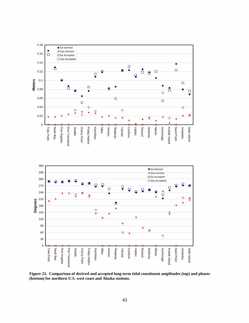
43

0

0.02

0.04

0.06

0.08

0.1

0.12

0.14

0.16

0.18

Toke P

oin

t

Neah B

ay

Port A

ngele

s

Port T

ow

nsend

Seattle

Cherry

Poin

t

Frid

ay H

arb

or

Ketc

hik

an

Sitk

a

Juneau

Skagw

ay

Yakuta

t

Cord

ova

Vald

ez

Sew

ard

Seld

ovia

Nik

iski

Anchora

ge

Kodia

k Is

land

Sand P

oin

t

Unala

ska

Adak Is

land

Mete

rs

Sa Derived

Ssa Derived

Sa Accepted

Ssa Accepted

0

30

60

90

120

150

180

210

240

270

300

330

360

Toke

Po

int

Ne

ah

Ba

y

Po

rt An

ge

les

Po

rt Tow

nsen

d

Se

attle

Ch

erry

Po

int

Frid

ay H

arb

or

Ke

tch

ika

n

Sitk

a

Ju

ne

au

Ska

gw

ay

Ya

kuta

t

Co

rdo

va

Va

ldez

Se

wa

rd

Se

ldovia

Nik

iski

An

cho

rag

e

Ko

dia

k Is

land

Sa

nd

Po

int

Un

ala

ska

Ad

ak Is

land

Deg

rees

Sa Derived

Ssa Derived

Sa Accepted

Ssa Accepted

Figure 23. Comparison of derived and accepted long-term tidal constituent amplitudes (top) and phases

(bottom) for northern U.S. west coast and Alaska stations.

44

0

0.02

0.04

0.06

0.08

0.1

0.12

0.14

0.16

0.18

Mia

mi B

each

Vaca K

ey

Key W

est

Naple

s

Fort M

yers

St. P

ete

rsburg

Cle

arw

ate

r Beach

Cedar K

ey

Apala

chic

ola

Panam

a C

ity

Pensacola

Dauphin

Isla

nd

Gra

nd Is

le

Eugene Is

land

Sabin

e P

ass

Galv

esto

n P

ier 2

1

Galv

Ple

asure

Pie

r

Fre

eport

Rockport

Port M

ansfie

ld

Padre

Isla

nd

Port Is

abel

Mete

rs

Sa Derived

Ssa Derived

Sa Accepted

Ssa Accepted

0

30

60

90

120

150

180

210

240

270

300

330

360

Mia

mi B

ea

ch

Va

ca K

ey

Ke

y W

est

Na

ple

s

Fort M

ye

rs

St. P

ete

rsb

urg

Cle

arw

ate

r Be

ach

Ce

da

r Ke

y

Ap

ala

chic

ola

Pa

na

ma

City

Pe

nsa

cola

Da

up

hin

Isla

nd

Gra

nd

Isle

Eu

ge

ne

Isla

nd

Sa

bin

e P

ass

Ga

lve

sto

n P

ier 2

1

Ga

lv P

leasu

re P

ier

Fre

epo

rt

Ro

ckpo

rt

Po

rt Ma

nsfie

ld

Pa

dre

Isla

nd

Po

rt Isa

be

l

Deg

rees

Sa Derived

Ssa Derived

Sa Accepted

Ssa Accepted

Figure 24. Comparison of derived and accepted long-term tidal constituent amplitudes (top) and phases

(bottom) for Gulf of Mexico stations.

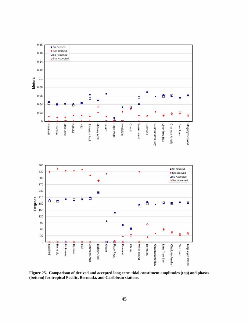
45

0

0.02

0.04

0.06

0.08

0.1

0.12

0.14

0.16

0.18

Naw

iliwili

Honolu

lu

Mokuolo

e

Kahulu

i

Hilo

Johnsto

n A

toll

Mid

way A

toll

Guam

Pago P

ago

Kw

aja

lein

Chuuk

Wake Is

land

Berm

uda

Guanta

nam

o B

ay

Lim

e T

ree B

ay

Charlo

tte A

malie

San J

uan

Magueyes Is

land

Mete

rs

Sa Derived

Ssa Derived

Sa Accepted

Ssa Accepted

0

30

60

90

120

150

180

210

240

270

300

330

360

Na

wiliw

ili

Ho

no

lulu

Mo

kuo

loe

Ka

hu

lui

Hilo

Jo

hn

sto

n A

toll

Mid

wa

y A

toll

Gu

am

Pa

go

Pa

go

Kw

aja

lein

Ch

uu

k

Wa

ke

Isla

nd

Be

rmu

da

Gu

an

tan

am

o B

ay

Lim

e T

ree B

ay

Ch

arlo

tte A

ma

lie

Sa

n J

uan

Ma

gu

eye

s Is

land

Deg

rees

Sa Derived

Ssa Derived

Sa Accepted

Ssa Accepted

Figure 25. Comparison of derived and accepted long-term tidal constituent amplitudes (top) and phases

(bottom) for tropical Pacific, Bermuda, and Caribbean stations.

46

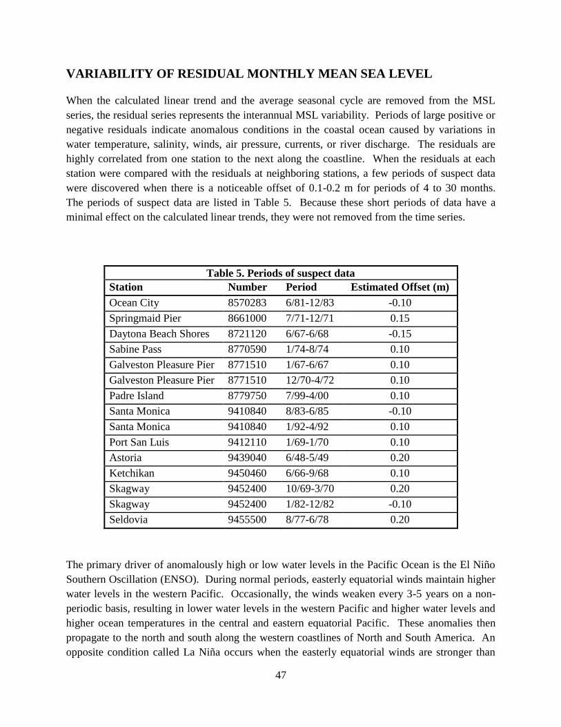
47

VARIABILITY OF RESIDUAL MONTHLY MEAN SEA LEVEL

When the calculated linear trend and the average seasonal cycle are removed from the MSL

series, the residual series represents the interannual MSL variability. Periods of large positive or

negative residuals indicate anomalous conditions in the coastal ocean caused by variations in

water temperature, salinity, winds, air pressure, currents, or river discharge. The residuals are

highly correlated from one station to the next along the coastline. When the residuals at each

station were compared with the residuals at neighboring stations, a few periods of suspect data

were discovered when there is a noticeable offset of 0.1-0.2 m for periods of 4 to 30 months.

The periods of suspect data are listed in Table 5. Because these short periods of data have a

minimal effect on the calculated linear trends, they were not removed from the time series.

Table 5. Periods of suspect data

Station Number Period Estimated Offset (m)

Ocean City 8570283 6/81-12/83 -0.10

Springmaid Pier 8661000 7/71-12/71 0.15

Daytona Beach Shores 8721120 6/67-6/68 -0.15

Sabine Pass 8770590 1/74-8/74 0.10

Galveston Pleasure Pier 8771510 1/67-6/67 0.10

Galveston Pleasure Pier 8771510 12/70-4/72 0.10

Padre Island 8779750 7/99-4/00 0.10

Santa Monica 9410840 8/83-6/85 -0.10

Santa Monica 9410840 1/92-4/92 0.10

Port San Luis 9412110 1/69-1/70 0.10

Astoria 9439040 6/48-5/49 0.20

Ketchikan 9450460 6/66-9/68 0.10

Skagway 9452400 10/69-3/70 0.20

Skagway 9452400 1/82-12/82 -0.10

Seldovia 9455500 8/77-6/78 0.20

The primary driver of anomalously high or low water levels in the Pacific Ocean is the El Niño

Southern Oscillation (ENSO). During normal periods, easterly equatorial winds maintain higher

water levels in the western Pacific. Occasionally, the winds weaken every 3-5 years on a non-

periodic basis, resulting in lower water levels in the western Pacific and higher water levels and

higher ocean temperatures in the central and eastern equatorial Pacific. These anomalies then

propagate to the north and south along the western coastlines of North and South America. An

opposite condition called La Niña occurs when the easterly equatorial winds are stronger than

48

normal leading to unusually high water levels in the western Pacific and low water levels and

temperatures in the central and eastern equatorial Pacific. During stronger ENSO events, the

effects are not confined to the Pacific basin but can propagate throughout the world via

atmospheric teleconnections.

The high correlation between ENSO and coastal water levels in the Pacific are demonstrated in

Figures 26 and 27. The Oceanic Niño Index (ONI) has become the standard method that

NOAA’s Climate Prediction Center uses in defining ENSO episodes (Climate Prediction Center

1999). It is based on a 3-month running mean of sea surface temperature in degrees in the Niño

3.4 region (5°N-5°S, 120°W-170°W) relative to a 1971-2000 base period. It has been divided by

a factor of 10 in Figures 26-27 for comparison with the water level residuals.

San Diego and most U.S. west coast and Alaska stations are highly correlated with the ONI.

Kwajalein in the western equatorial Pacific Ocean is also highly correlated with the ONI, but has

an opposite sign; when the ONI is high, Kwajalein has low water levels and when the ONI is

low, Kwajalein has high water levels. The Pacific island stations at Guam, Pago Pago, and

Chuuk are also inversely correlated with the ONI. In contrast, the Hawaiian stations, Johnston

Atoll, Midway Atoll, and Wake Island are not correlated with the ONI.

Since residual MSLs are highly correlated from station to station along a coastline, they

represent regional anomalous conditions in the coastal ocean. In order to highlight extremes in

coastal ocean conditions and to determine the geographical extent of such events, an anomaly

threshold of 0.1 m was applied to the 5-month average of the monthly MSL residuals (Zervas

2001). A positive anomaly was defined to occur when the 5-month average is above 0.1 m; a

negative anomaly was defined to occur when the 5-month average is below -0.1 m.

The number of months each year with extreme residual MSLs are listed in Table 6 for the

Atlantic stations and Table 7 for the Pacific stations. The years with monthly residuals above 0.1

m are positive and are shaded red. The years with monthly residuals below -0.1 m are negative

and are shaded blue. Years with no extreme monthly residuals are indicated by a zero. Years

without data are blank. The periods of suspect data in Table 5 are not included in Tables 6 and 7.

Tables 6 and 7 indicate the time periods and the regional extent of MSL anomalies for the past

100 years.

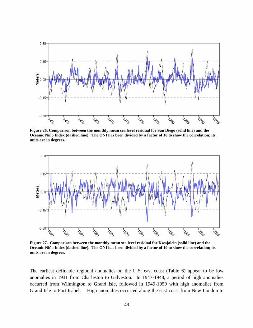
49

Figure 26. Comparison between the monthly mean sea level residual for San Diego (solid line) and the

Oceanic Niño Index (dashed line). The ONI has been divided by a factor of 10 to show the correlation; its

units are in degrees.

Figure 27. Comparison between the monthly mean sea level residual for Kwajalein (solid line) and the

Oceanic Niño Index (dashed line). The ONI has been divided by a factor of 10 to show the correlation; its

units are in degrees.

The earliest definable regional anomalies on the U.S. east coast (Table 6) appear to be low

anomalies in 1931 from Charleston to Galveston. In 1947-1948, a period of high anomalies

occurred from Wilmington to Grand Isle, followed in 1949-1950 with high anomalies from

Grand Isle to Port Isabel. High anomalies occurred along the east coast from New London to

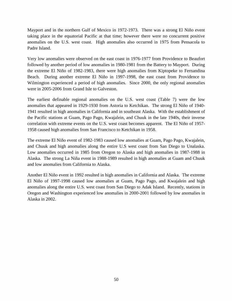
50

Mayport and in the northern Gulf of Mexico in 1972-1973. There was a strong El Niño event

taking place in the equatorial Pacific at that time; however there were no concurrent positive

anomalies on the U.S. west coast. High anomalies also occurred in 1975 from Pensacola to

Padre Island.

Very low anomalies were observed on the east coast in 1976-1977 from Providence to Beaufort

followed by another period of low anomalies in 1980-1981 from the Battery to Mayport. During

the extreme El Niño of 1982-1983, there were high anomalies from Kiptopeke to Fernandina

Beach. During another extreme El Niño in 1997-1998, the east coast from Providence to

Wilmington experienced a period of high anomalies. Since 2000, the only regional anomalies

were in 2005-2006 from Grand Isle to Galveston.

The earliest definable regional anomalies on the U.S. west coast (Table 7) were the low

anomalies that appeared in 1929-1930 from Astoria to Ketchikan. The strong El Niño of 1940-

1941 resulted in high anomalies in California and in southeast Alaska. With the establishment of

the Pacific stations at Guam, Pago Pago, Kwajalein, and Chuuk in the late 1940s, their inverse

correlation with extreme events on the U.S. west coast becomes apparent. The El Niño of 1957-

1958 caused high anomalies from San Francisco to Ketchikan in 1958.

The extreme El Niño event of 1982-1983 caused low anomalies at Guam, Pago Pago, Kwajalein,

and Chuuk and high anomalies along the entire U.S west coast from San Diego to Unalaska.

Low anomalies occurred in 1985 from Oregon to Alaska and high anomalies in 1987-1988 in

Alaska. The strong La Niña event in 1988-1989 resulted in high anomalies at Guam and Chuuk

and low anomalies from California to Alaska.

Another El Niño event in 1992 resulted in high anomalies in California and Alaska. The extreme

El Niño of 1997-1998 caused low anomalies at Guam, Pago Pago, and Kwajalein and high

anomalies along the entire U.S. west coast from San Diego to Adak Island. Recently, stations in

Oregon and Washington experienced low anomalies in 2000-2001 followed by low anomalies in

Alaska in 2002.

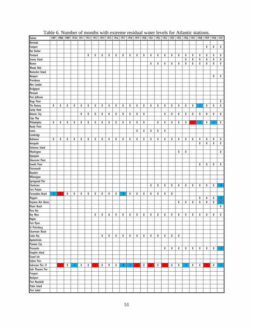
51

Table 6. Number of months with extreme residual water levels for Atlantic stations. Station 1907 1908 1909 1910 1911 1912 1913 1914 1915 1916 1917 1918 1919 1920 1921 1922 1923 1924 1925 1926 1927 1928 1929 1930 1931

Bermuda

Eastport 0 0 0

Bar Harbor

Portland 0 0 0 0 0 0 0 0 0 0 0 0 0 0 0 0 0 0 0 0

Seavey Island 0 0 0 0 0 0

Boston 0 0 0 0 0 0 0 0 0 0 0

Woods Hole

Nantucket Island

Newport 0 0

Providence

New London

Bridgeport

Montauk

Port Jefferson

Kings Point 0

The Battery 0 0 0 0 0 0 0 0 0 0 0 0 0 0 0 0 0 0 0 0 0 -1 0 0 0

Sandy Hook

Atlantic City 0 0 0 0 0 0 0 0 0 0 0 0 0 0 0 0 0 0 0

Cape May

Philadelphia 0 0 0 0 0 0 0 0 0 0 0 0 0 0 0 0 0 0 0 1 -1 0 -1 0

Reedy Point

Lewes 0 0 0 0 0

Cambridge

Baltimore 0 0 0 0 0 0 0 0 0 0 0 0 0 0 0 0 0 0 0 0 0 0 0 0 0

Annapolis 0 0 0 0

Solomons Island

Washington 0 0 0

Kiptopeke

Gloucester Point

Sewells Point 0 0 0 0

Portsmouth

Beaufort

Wilmington

Springmaid Pier

Charleston 0 0 0 0 0 0 0 0 0 0 -4

Fort Pulaski

Fernandina Beach -2 2 0 0 0 0 0 0 0 0 -4 0 0 0 0 0 0 0

Mayport 0 0 0 -4

Daytona Bch Shores 0 0 0 0 0 0 -1

Miami Beach 0

Vaca Key

Key West 0 0 0 0 0 0 0 0 0 0 0 0 0 0 0 0 0 0 0

Naples

Fort Myers

St Petersburg

Clearwater Beach

Cedar Key 0 0 0 0 0 0 0 0 0 0 0 0

Apalachicola

Panama City

Pensacola 0 0 0 0 0 0 0 0 -3

Dauphin Island

Grand Isle

Sabine Pass

Galveston Pier 21 2 0 -1 0 0 1 0 0 0 -4 -1 1 0 6 0 2 0 0 -1 0 0 2 0 -7

Galv Pleasure Pier

Freeport

Rockport

Port Mansfield

Padre Island

Port Isabel

52

Table 6. Number of months with extreme residual water levels for Atlantic stations. Station 1932 1933 1934 1935 1936 1937 1938 1939 1940 1941 1942 1943 1944 1945 1946 1947 1948 1949 1950 1951 1952 1953 1954 1955 1956

Bermuda 0 0 0 0 0 0 0 0 0 -1 -3 0 0 0 0 0 0 0 0 4 1

Eastport 0 0 0 0 0 0 0 0 0 0 0 0 0 0 0 0 0 0 0 0 0 0 0 0 0

Bar Harbor 0 0 0 0 0 0 0 0 0 0

Portland 0 0 0 0 0 0 0 0 0 0 0 0 0 0 0 0 0 0 0 0 0 0 0 0 0

Seavey Island 0 0 0 0 0 0 0 0 0 0 0 0 0 0 0 0 0 0 0

Boston 0 0 0 0 0 0 0 0 0 0 0 0 0 0 0 0 0 0 0 0 0 0 0 0 0

Woods Hole 0 0 0 0 0 0 0 0 0 0 0 0 0 0 0 0 0 0 0 0 0 0 0 0 0

Nantucket Island

Newport 0 0 0 0 0 0 0 0 0 0 0 0 0 0 0 0 0 0 0 0 0 0 0 0 0

Providence 0 0 0 0 0 0 0 0 0 0

New London 0 0 0 0 0 0 0 0 0 0 0 0 0 0 0 0 0 0 0

Bridgeport

Montauk 0 0 0 0 0 0 0 0 0 0

Port Jefferson

Kings Point 0 0 0 0 0 0 0 0 0 0 0 0 0 0 0 0 0 0 0 0 0 0 0 0 0

The Battery 0 0 0 0 0 0 0 0 0 0 0 0 0 0 0 0 0 0 0 0 0 0 0 0 0

Sandy Hook 0 0 0 0 0 0 0 0 0 0 0 0 0 0 0 0 0 0 0 0 0 0 0 0

Atlantic City 0 0 0 0 0 0 0 0 0 0 0 0 0 0 0 0 0 0 0 0 0 0 0 0 0

Cape May

Philadelphia 0 0 0 0 1 0 0 0 0 0 0 0 0 0 0 0 1 0 0 0 0 2 0 0 0

Reedy Point 0

Lewes 0 0 0 0 0 0 0 0 0 0 0 0

Cambridge 0 0 0 0 0 0 0 0 0

Baltimore 0 0 0 0 0 0 0 0 0 0 0 0 0 0 0 0 0 0 0 0 0 0 0 0 0

Annapolis 0 0 0 0 0 0 0 0 0 0 0 0 0 0 0 0 0 0 0 0 0 0 0 0 0

Solomons Island 0 0 0 0 0 0 0 0 0 0 0 0 0 0 0 0 0 0 0

Washington 0 0 0 0 2 0 0 0 0 0 0 0 0 0 0 0 2 0 -1 0 0 0 0 0 0

Kiptopeke 0 0 0 0 0 0

Gloucester Point 0 0 0 0 0 0 0

Sewells Point 0 0 0 0 0 0 0 0 0 0 0 0 0 0 0 0 0 0 0 0 0 0 0 0 0

Portsmouth 0 0 0 0 0 0 0 0 0 0 0 0 0 0 0 0 0 0 0 0 0 0

Beaufort 0 0 0 0

Wilmington 0 0 1 0 0 0 -3 0 0 0 4 0 3 5 0 0 0 0 0 0 1 0

Springmaid Pier

Charleston 0 0 0 0 0 0 0 0 0 0 0 0 0 0 0 3 8 0 0 0 0 0 0 0 0

Fort Pulaski 0 0 0 0 0 0 0 0 0 0 0 0 4 5 0 0 0 0 0 0 0 0

Fernandina Bch 0 0 0 0 0 0 0 0 3 4 0 0 0 0 0 0 0 0

Mayport 0 0 0 0 0 0 0 0 0 0 0 0 0 0 0 3 6 0 0 0 0 0 0 0 0

Daytona Bch Shores 0 0 0 0 0 0 0 0 0 0 3 6 0 0

Miami Beach 0 0 0 0 0 0 0 0 0 0 0 0 0 0 0 2 6 0 0 0 0 0

Vaca Key

Key West 0 0 0 0 0 0 0 0 0 0 0 0 0 0 0 1 3 0 0 0 0 0 0 0 0

Naples

Fort Myers

St Petersburg 0 4 0 0 0 0 0 0 0 0

Clearwater Beach

Cedar Key 0 0 0 0 0 0 0 0 0 0 4 1 0 0 0 0 0 0 0

Apalachicola

Panama City

Pensacola 0 0 0 0 0 0 0 0 0 0 0 0 0 0 0 0 5 0 0 0 0 0 0 0 0

Dauphin Island

Grand Isle 0 2 1 1 0 0 0 0 0 0

Sabine Pass

Galveston Pier 21 0 0 0 0 0 0 0 -2 -6 0 0 0 0 1 3 0 0 2 3 0 0 0 0 0 0

Galv Pleasure Pier

Freeport -3 -1 0

Rockport 0 2 3 0 0 0 0

Port Mansfield

Padre Island

Port Isabel 0 0 3 0 1 0 1 0 0 0 0 0 0

53

Table 6. Number of months with extreme residual water levels for Atlantic stations. Station 1957 1958 1959 1960 1961 1962 1963 1964 1965 1966 1967 1968 1969 1970 1971 1972 1973 1974 1975 1976 1977 1978 1979 1980 1981

Bermuda 4 2 0 0 2 5 0 0 0 0 0 0 -1 -6 -3 0 -2 3 3 1 0 0 0 0 0

Eastport 0 0 0 0 0 0 0 0 0 0 0 1 0 2 0 0 0 0 0 0 0 0 0

Bar Harbor 0 0 0 0 0 0 0 0 0 0 0 0 0 0 0 0 0 0 0 0 0 0

Portland 0 0 0 0 0 0 0 0 0 0 0 0 0 3 2 0 0 0 0 0 0 0 0 0 0

Seavey Island 0 0 0 0 0 0 0 0 0 0 0 0 0 0 0 0 0 0 0 0 0 0 0 0 0

Boston 0 1 0 0 0 0 0 0 0 0 0 0 0 0 0 0 0 0 0 0 0 0 0 0 0

Woods Hole 0 0 0 0 0 0 0 0 0 0 0 0 0 0 0 0 0 0 0 0 0 0 0

Nantucket Island 0 0 0 0 0 0 0 0 0 0 0 0 0 0 0 0 0

Newport 0 0 0 0 0 0 0 0 0 0 0 0 0 0 0 0 0 0 0 0 0 0 0 0 0

Providence 0 0 0 0 0 0 0 0 0 0 0 0 0 0 0 0 0 0 -1 -2 0 0 0 0

New London 0 0 0 0 0 0 0 0 0 0 0 0 0 0 0 0 1 0 0 0 0 0 -1 0

Bridgeport 0 0 0 0 0 0 0 2 0 0 -2 -2 0 0 0 0

Montauk 0 2 0 0 0 0 0 0 0 0 0 0 0 0 0 0 0 0 0 0 0 0 0 0

Port Jefferson 0 0 0 0 0 0 0 0 0 0 0 0 0 0 0 0 0 0 0 -2 -2 0 0 0 0

Kings Point 0 0 0 0 0 0 0 0 0 0 0 0 0 0 0 1 3 0 0 -2 -2 0 0 0 0

The Battery 0 0 0 0 0 0 0 0 0 0 0 0 0 0 0 0 1 0 0 -2 -3 0 0 -2 -1

Sandy Hook 0 0 0 0 0 0 0 0 0 0 0 0 0 0 0 1 3 0 0 -2 -3 0 0 0 0

Atlantic City 0 0 0 0 0 0 0 0 0 0 0 0 0 0 1 3 0 0 0 -1 0 0 -2 -1

Cape May 0 0 0 1 3 0 0 0 0 0 0 0

Philadelphia 0 0 0 0 0 0 0 0 0 0 0 0 0 0 1 4 0 0 -2 -3 0 0 -3 -2

Reedy Point -1 0 0 4 0 0 0 0 0 0 -2 -3

Lewes 0 0 0 0 0 0 0 0 0 0 0 0 0 0 0 2 4 0 0 -2 -4 0 0 0 0

Cambridge 0 0 2 0 0 0 0 0 0 0

Baltimore 0 0 0 0 0 0 0 0 0 0 0 0 0 0 0 0 2 0 0 -2 -3 0 0 -2 0

Annapolis 0 0 0 0 0 0 0 0 0 0 0 0 0 0 0 0 1 0 0 -2 0 0 0 0

Solomons Island 0 0 0 0 0 0 0 0 0 0 0 0 0 0 0 0 1 0 0 -2 0 0 -2 -2

Washington 0 0 0 0 0 0 0 0 0 0 0 0 0 0 0 7 3 0 0 -1 -4 0 0 -2 -5

Kiptopeke 0 0 0 0 0 0 0 0 0 0 0 0 0 0 0 0 1 0 0 -2 -4 0 0 0 0

Gloucester Point 0 0 0 0 0 0 0 0 0 0 0 0 0 0 1 2 0 0 -2 -4 0 0 -1 -1

Sewells Point 0 0 0 0 0 0 0 0 0 0 0 0 0 0 0 2 3 0 0 -2 -4 0 0 -2 -1

Portsmouth 0 0 0 0 0 0 0 0 0 0 0 0 0 0 0 1 2 0 0 -2 -4 0 0 -1 -1

Beaufort 0 0 0 0 0 0 0 0 0 0 0 0 -1 -2 0 0 -1 0

Wilmington 0 0 0 0 0 0 0 0 0 0 0 0 0 0 0 1 4 0 0 0 0 0 0 -4 -2

Springmaid Pier 0 0 0 0 0 0 0 0 0 0 0 1 1 0 0 0 0 0 0

Charleston 0 0 0 0 0 0 0 0 0 0 0 0 0 0 0 1 3 0 0 0 0 0 0 0 0

Fort Pulaski 0 0 0 0 0 0 0 0 0 0 0 0 0 0 0 0 0 0 0 0 0 0 0

Fernandina Bch 0 0 0 0 0 0 0 0 0 0 0 0 0 0 0 0 2 0 0 0 0 0 0 -1 0

Mayport 0 0 0 1 0 0 0 0 0 0 0 0 0 0 0 0 2 0 0 0 0 0 0 -5 0

Daytona Bch Shores 0 0 0 0 1 0 0 0 0 0 0 0

Miami Beach 0 0 0 0 0 0 0 0 0 0 0 0 0 0 0 0 0 0 0 0 0 0 0 0 0

Vaca Key 0 0 0 0 0 0 0 0 0 0 0

Key West 0 0 0 0 0 0 0 0 0 0 0 0 0 0 0 0 0 0 0 0 0 0 0 0 0

Naples 0 0 0 0 0 0 0 0 0 0 0 0 0 0 0 0 0

Fort Myers 0 0 0 0 0 0 0 0 0 0 0 0 0 0 0 0 0

St Petersburg 0 0 0 0 0 0 0 0 0 0 0 0 0 0 0 0 0 0 0 0 0 0 0 0 0

Clearwater Beach 0 0 0 0 0 0 0 0 0

Cedar Key 0 0 0 0 1 1 0 0 0 0 0 0 0 0 0 0 0 0 0 0 0 0 0 0 0

Apalachicola 0 0 0 0 0 4 0 0 0 0 0 0 0

Panama City 0 0 0 0 0 0 0 0 0

Pensacola 0 0 0 0 0 0 0 0 0 0 0 0 0 0 0 0 2 0 5 0 0 0 0 0 0

Dauphin Island 0 0 0 0 0 0 0 -1 0 0 0 0 0

Grand Isle 0 0 0 0 0 0 -3 -2 0 0 0 0 0 0 0 0 2 0 5 0 0 0 0 0

Sabine Pass 0 0 0 0 0 -7 -5 -3 0 0 0 0 -1 1 2 2 7 0 0 0

Galveston Pier 21 0 0 0 0 2 0 -4 -3 0 0 0 0 0 0 -2 0 1 0 5 -1 0 0 3 0 0

Galv Pleasure Pier 0 0 0 0 1 0 -1 -9 0 0 0 0 0 1 0 0 -7 -1

Freeport 0 0 0 0 2 0 0 -1 0 0 0 0 0 0 2 0 0 0 3 -4 0 0 0 0 0

Rockport -1 -4 0 0 0 0 0 0 1 0 0 0 4 0 0 0 0 -2 0

Port Mansfield -1 0 -1 1 2 5 0 0 5 0 0 0 0 -1 0

Padre Island 0 0 0 0 0 -1 0 0 0 0 0 0 0 0 0 0 5 -3 0 0

Port Isabel 0 0 0 0 1 0 0 -1 0 0 0 0 0 0 0 0 0 0 0 0 0 0 0 0

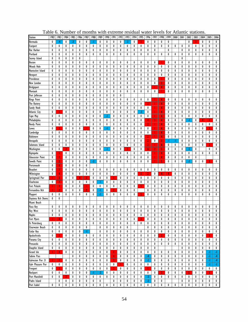
54

Table 6. Number of months with extreme residual water levels for Atlantic stations. Station 1982 1983 1984 1985 1986 1987 1988 1989 1990 1991 1992 1993 1994 1995 1996 1997 1998 1999 2000 2001 2002 2003 2004 2005 2006

Bermuda 0 -4 0 -2 0 0 -1 0 0 0 0 -3 0 2 0 0 0 0 0 3 0 0 0

Eastport 0 0 0 0 0 0 0 0 0 0 0 0 0 0 0 0 0 0 0 0 0 0 0 0 0

Bar Harbor 0 0 0 0 0 0 0 0 0 0 0 0 0 0 0 0 0 0 0 0 0 0 0

Portland 0 0 0 0 0 0 0 0 0 0 0 0 0 0 0 0 0 0 0 0 0 0 0 0 0

Seavey Island 0 0 0 0 0 0

Boston 0 0 0 0 0 0 0 0 0 0 0 0 0 0 0 0 1 0 0 0 0 0 0 0 0

Woods Hole 0 0 0 0 0 0 0 0 0 0 0 0 0 0 0 0 0 0 0 0 0 0 0 0 0

Nantucket Island 0 0 0 0 0 0 0 0 0 0 0 0 0 0 0 0 0 0 0 0 0 0 0 0 0

Newport 0 0 0 0 0 0 0 0 0 0 0 0 0 0 0 0 0 0 0 0 0 0 0 0 0

Providence 0 0 0 0 0 0 0 0 0 0 0 0 0 0 0 0 1 0 0 0 0 0 0 0 0

New London 0 0 0 0 0 0 0 0 0 0 0 0 0 0 0 0 3 0 0 0 0 0 0 0 0

Bridgeport 0 0 0 0 0 0 0 0 0 0 0 0 0 0 0 1 4 0 0 0 0 0 0 0 0

Montauk 0 0 0 0 0 0 0 0 0 0 0 0 0 0 0 0 1 0 0 0 0 0 0 0 0

Port Jefferson 0 0 0 0 0 0 0 0 0 0 0

Kings Point 0 0 0 0 0 0 0 0 0 0 0 0 0 0 0 1 4 0 0 0 0 0 0 0 0

The Battery 0 0 0 0 0 0 0 0 0 0 0 0 0 0 2 1 4 0 0 0 0 0 0 0 0

Sandy Hook 0 0 0 0 0 0 0 0 0 0 0 0 0 0 0 1 4 0 0 0 0 0 0 0 0

Atlantic City 0 1 0 0 0 0 0 0 0 0 0 0 0 -3 0 1 4 0 0 0 0 0 0 0 0

Cape May 0 0 0 0 0 0 0 0 -1 0 0 0 0 0 0 1 4 0 0 0 0 0 0 0 0

Philadelphia 0 0 0 0 0 0 0 0 0 0 0 0 0 0 4 3 4 0 0 0 -1 0 4 3 0

Reedy Point 0 0 0 0 0 0 0 0 0 0 0 0 0 0 2 1 4 0 0 0 0 0 0 0 0

Lewes 0 1 0 0 0 1 0 0 -1 0 0 0 0 0 0 1 4 0 0 0 0 0 0 1 0

Cambridge 0 0 0 0 0 0 0 0 0 0 0 0 0 0 0 1 4 0 0 0 0 0 0 0 0

Baltimore 0 0 0 0 0 0 0 0 0 0 0 0 0 0 2 1 4 0 0 0 0 0 0 0 0

Annapolis 0 0 0 0 0 0 0 0 0 0 0 0 0 0 2 0 3 -1 -1 0 0 0 0 0 0

Solomons Island 0 0 0 0 0 0 0 0 0 0 0 0 0 0 2 1 4 0 0 0 0 0 0 2 0

Washington 0 0 2 0 0 0 0 0 -1 0 0 2 0 0 6 2 5 0 0 0 -5 0 0 0

Kiptopeke 0 1 0 0 0 0 0 0 0 0 0 0 0 0 0 1 4 0 0 0 0 0 0 0 0

Gloucester Point 0 1 0 0 0 0 0 0 0 0 0 0 0 0 0 1 4 0 0 0 0 0

Sewells Point 0 2 0 0 0 0 -3 0 0 0 0 0 0 0 0 1 5 0 0 0 -1 0 0 1 0

Portsmouth 0 4 0 0 0 0

Beaufort 0 2 0 0 0 0 0 0 0 0 0 0 0 0 0 0 0 0 0 0 0 0 0 0 0

Wilmington 0 4 0 0 0 0 0 0 0 0 0 0 0 1 2 0 4 4 0 0 0 0 0 0 0

Springmaid Pier 1 2 0 0 4 3 0 0 0 1 0 0 0 0 0 0 0 0 0 0 0 0 0 0 0

Charleston 0 2 0 0 0 0 0 -1 0 0 0 0 0 0 0 0 0 0 0 0 0 0 0 0 0

Fort Pulaski 1 2 0 0 0 1 0 0 0 0 0 0 0 5 0 0 0 0 0 0 0 0 0 0 0

Fernandina Bch 1 2 0 0 0 2 0 -1 0 2 0 0 0 0 0 0 0 0 0 0 0 0 0 0

Mayport 0 0 0 0 0 0 0 -1 0 0 0 0 0 5 0 0 0 0 0 0 0 0 0 0 0

Daytona Bch Shores 0 0

Miami Beach

Vaca Key 0 0 0 0 0 0 0 0 0 0 0 0 0 0 0 0 0 0 0 0 0 0 0 0 0

Key West 0 0 0 0 0 0 0 0 0 0 0 0 0 0 0 0 0 0 0 0 0 0 0 0 0

Naples 0 0 0 0 0 0 0 0 0 0 0 0 0 0 0 0 0 0 0 0 0 0 0 0 0

Fort Myers 1 4 0 0 0 0 0 0 0 0 0 0 0 3 0 0 0 0 0 0 0 0 0 0 0

St Petersburg 0 0 0 0 0 0 0 0 0 0 0 0 0 0 0 0 0 0 0 0 0 0 0 0 0

Clearwater Beach 0 0 0 0 0 0 0 0 0 0 0 0 0 0 0 0 0 0 0 0 0 0

Cedar Key 0 0 0 0 0 -1 0 0 0 0 0 0 0 0 0 0 0 0 0 0 0 0 0 0

Apalachicola 0 1 0 0 0 0 0 0 0 0 0 0 0 0 0 0 3 0 0 0 0 0 0 1 0

Panama City 0 0 0 0 0 0 0 0 0 0 0 0 0 0 0 0 0 0 0 0 0 0 0 0 0

Pensacola 0 0 0 0 0 0 0 0 0 0 0 0 0 0 0 0 0 0 0 0 0 0 0 0 0

Dauphin Island 0 0 0 0 0 0 0 0 0 0 0 0 0 0 0 0 0 0 0 0 0 0

Grand Isle 1 3 0 0 0 0 0 0 0 1 0 0 0 0 0 0 0 0 0 0 0 0 0 -1 -1

Sabine Pass 0 0 0 0 0 0 4 0 0 0 0 -4 0 0 0 0 0 0 0 0 -1 -4

Galveston Pier 21 1 1 0 0 0 0 0 0 0 3 0 0 0 0 -1 0 0 0 0 0 0 0 0 -1 -4

Galv Pleasure Pier 0 0 0 0 0 0 0 0 0 0 1 0 0 0 0 0 0 0 0 0 0 0 0 -1 -1

Freeport 0 1 0 0 0 0 0 0 0 3 0 0 0 0 1 0 0 0 0 0 0 0 0 0 0

Rockport 0 0 0 0 0 0 -1 -2 0 0 0 0 0 0 0 0 3 0 0 0 5 0 0 1 0

Port Mansfield 0 0 2 0 0 0 0 0 0 0 0 0 0 0 -3 0 0 0 0 0 0 0 0 0 0

Padre Island 0 0 0 0 0 0 0 0 0 0 0 0 -2 0 0 0 0 0 0 0 0

Port Isabel 0 0 0 0 0 0 0 0 0 0 0 0 0 0 0 0 0 0 0 0 0 0 0 0 0

55

Table 7. Number of months with extreme residual water levels for Pacific stations. Station 1907 1908 1909 1910 1911 1912 1913 1914 1915 1916 1917 1918 1919 1920 1921 1922 1923 1924 1925 1926 1927 1928 1929 1930 1931

Nawiliwili

Honolulu 0 0 -6 -2 0 0 0 0 2 0 0 0 0 7 0 0 0 0 0 0 0 0 0 0 0

Mokuoloe

Kahului

Hilo 0 0 0 0 0

Johnston Atoll

Midway Atoll

Guam

Pago Pago

Kwajalein

Chuuk

Wake Island

San Diego 0 0 0 0 0 0 0 0 0 0 0 0 0 0 0 0 0 0 0 0 0 0 0 0 0

La Jolla 0 0 0 0 0 0 0

Newport Beach

Los Angeles 0 0 0 0 0 0 0 0

Santa Monica

Rincon Island

Santa Barbara

Port San Luis

Monterey

San Francisco 0 0 0 0 0 0 0 1 2 0 0 0 0 0 0 0 0 0 0 0 0 0 0 0 0

Redwood City

Alameda

Point Reyes

Port Chicago

North Spit

Crescent City

Port Orford

Charleston

South Beach

Garibaldi

Astoria 0 0 2 -1 -6 -1 0

Toke Point

Neah Bay

Port Angeles

Port Townsend

Seattle 0 0 0 0 0 0 0 0 0 0 0 0 0 0 0 0 0 0 0 0 0 0 -4 -1 0

Cherry Point

Friday Harbor

Ketchikan -1 0 0 0 0 0 0 1 0 0 -2 -1 3

Sitka 0 0 0

Juneau

Skagway

Yakutat

Cordova

Valdez

Seward 0 5 0 0 0 1 3

Seldovia

Nikiski

Anchorage

Kodiak Island

Sand Point

Unalaska

Adak Island

56

Table 7. Number of months with extreme residual water levels for Pacific stations. Station 1932 1933 1934 1935 1936 1937 1938 1939 1940 1941 1942 1943 1944 1945 1946 1947 1948 1949 1950 1951 1952 1953 1954 1955 1956

Nawiliwili -1 0

Honolulu 0 0 0 0 0 0 0 0 0 0 0 1 0 0 0 0 0 0 0 0 0 0 0 -3 0

Mokuoloe

Kahului 0 0 0 0 0 0 0 -2 0

Hilo 0 0 0 0 0 0 0 0 0 0 0

Johnston Atoll 0 0 0 0 0 0 0 0

Midway Atoll 0 0 0 0 1 0 0 0 0 0

Guam 0 0 1 0 0 2 3 0 0

Pago Pago 0 0 0 0 0 0 0 2

Kwajalein 0 0 0 0 0 0 0 0 0 0 0

Chuuk 0 0 0 0 3 1

Wake Island 0 0 1 4 0 0 0

San Diego 0 0 0 0 0 0 0 0 0 0 0 0 0 0 0 0 0 0 0 0 0 0 0 0 0

La Jolla 0 0 0 0 0 0 0 0 0 0 0 0 0 0 0 0 0 0 0 0 0 0 0 0

Newport Beach 0 0

Los Angeles 0 0 0 0 0 0 0 0 0 2 0 0 0 0 0 0 0 0 0 0 0 0 0 0 0

Santa Monica -1 0 0 0 0 0 0 0 2 0 0 0 0 0 0 0 0 0 0 0 0 0 0 0

Rincon Island

Santa Barbara

Port San Luis 0 -1 0 0 0 0 0 0 0 0 0 0

Monterey

San Francisco 0 0 0 0 0 0 0 0 1 4 0 0 0 0 0 0 0 0 0 0 0 0 0 0 0

Redwood City

Alameda 0 1 5 0 0 0 0 0 0 0 0 0 0 0 0 0 0 0

Point Reyes

Port Chicago

North Spit

Crescent City 0 0 0 0 0 -1 -2 1 4 0 0 0 0 0 0 0 0 0 0 0 0 0

Port Orford

Charleston

South Beach

Garibaldi

Astoria 0 1 0 0 -3 -1 -1 -2 0 0 0 0 -5 -1 0 0 1 0 0 0 0 -1 -2

Toke Point

Neah Bay 0 0 -3 -1 0 -2 0 0 0 0 0 0 0 0 0 0 0 0 0 0 0 0 -1

Port Angeles

Port Townsend

Seattle 0 0 0 0 -2 0 0 -2 0 0 0 0 0 0 0 0 0 0 0 0 0 0 0 0 0

Cherry Point

Friday Harbor 0 0 0 0 0 -1 0 1 0 0 0 0 0 0 0 0 0 0 0 0 0 0 0

Ketchikan 0 0 0 0 0 0 0 0 2 1 0 0 0 0 0 0 0 0 0 0 0 0 0 0 -1

Sitka 0 0 2 1 0 0 0 0 -1 -1 0 0 0 0 0 0 0 0 -2

Juneau 0 0 0 2 2 0 0 -1 -1 0 0 0 0 0 0 0 0 -3

Skagway 0 0 -1 0 0 0 -1 -3 2 2 0 -2 -4

Yakutat 0 0 0 0 0 0 -2 -1 0 0 0 0 0 0 0 -1 -4

Cordova 0 0 0

Valdez

Seward 0 0 0 0 -1 0 0 0 0 0 0 0 0 0 0 3 2 0 -1 -2

Seldovia

Nikiski

Anchorage

Kodiak Island 0 0 0 1 0 0 -2

Sand Point

Unalaska 0 0 0 -2 0 0 0 0 0 0 0 0 2 3 0 0 0

Adak Island 0 0 0 0 0 0 0 0 0 0 0 0 0 0

57

Table 7. Number of months with extreme residual water levels for Pacific stations. Station 1957 1958 1959 1960 1961 1962 1963 1964 1965 1966 1967 1968 1969 1970 1971 1972 1973 1974 1975 1976 1977 1978 1979 1980 1981

Nawiliwili 0 0 0 0 0 0 0 0 0 0 0 0 0 0 0 0 0 0 0 0 0 0 0 0 0

Honolulu 0 0 0 0 0 0 0 0 0 0 0 0 0 0 0 0 0 0 0 0 0 0 0 0 0

Mokuoloe 0 0 0 0 0 0 0 0 0 0 0 0 0 0 0

Kahului 0 0 0 0 2 0 0 0 0 0 0 0 0 0 0 0 0 0 0 0 0 0 0 0

Hilo 0 0 0 0 4 0 0 0 0 0 0 0 0 0 0 0 0 0 0 0 0 0 0 0 0

Johnston Atoll 1 0 0 0 4 0 0 0 0 0 0 0 0 1 0 0 0 0 0 0 0 -1 -2 0 0

Midway Atoll 0 0 0 0 0 0 0 2 0 0 0 0 -2 0 0 0 0 -1 0 0 -2 0 0 -3

Guam 0 0 -1 0 0 0 0 0 0 0 -1 -3 -2 5 6 -7 0 1 0 0 0 0 0 4

Pago Pago 0 -1 0 0 0 0 0 0 0 0 0 0 0 0 4 0 0 0 0 0 0 -1 0 0 0

Kwajalein -2 -1 0 0 0 0 0 0 0 0 0 0 0 0 0 -1 0 0 0 0 0 0 0 0 0

Chuuk -3 -2 0 0 0 0 -1 0 -4 -1 0 0 0 0 1 -7 2 0 1 0 0 0 0 0 0

Wake Island 0 0 0 1 0 0 0 0 0 -2 0 0 0 0 0 0 0 0 0 0 0 0

San Diego 0 0 0 0 0 0 0 0 0 0 0 0 0 0 0 0 0 0 0 0 0 0 0 0 0

La Jolla 0 0 0 0 0 0 0 0 0 0 0 0 0 0 0 0 0 0 0 0 0 0 0 0 0

Newport Beach 0 0 0 0 0 0 0 0 0 0 0 0 0 0 0 0 0 0 0 0 0 0 0 0 0

Los Angeles 0 0 0 0 0 0 0 0 0 0 0 0 0 0 0 0 0 0 0 0 0 0 0 0 0

Santa Monica 0 1 0 0 0 0 0 0 0 0 0 0 0 0 0 0 0

Rincon Island 0 0 0 0 0 0 0 0 0 0 0 0 0 0 0 0 0 0

Santa Barbara 0 0 0 0 0 0 0

Port San Luis 0 0 0 0 0 0 0 0 0 0 0 0 0 0 0 0 0 0 0 0 0 0

Monterey 0 0 0 0 0 0 0 0

San Francisco 0 3 0 0 0 0 0 0 0 0 0 0 0 0 0 1 0 0 0 0 -3 0 0 0 0

Redwood City 0 0

Alameda 0 3 0 0 0 0 0 0 0 0 0 0 0 0 0 0 0 0 -2 -2 -2 0 0 0 0

Point Reyes 0 -1 0 0 0 0 0

Port Chicago -4 0 0 0 0

North Spit 0 0 0 0

Crescent City 1 4 0 0 0 0 0 -2 0 0 0 0 0 0 0 0 0 0 0 -2 0 1 0 0 0

Port Orford 1 0

Charleston 0 0 0 0 0 0 0 1 2 0 0 0

South Beach 0 1 0 0 0 0 0 0 0 0 -3 0 0 0 0

Garibaldi 0 0 0 0 0 0 -1 -2 0 0 0

Astoria -1 2 0 0 -2 -1 0 -2 0 0 0 1 1 -2 0 2 -4 2 0 -1 -6 -2 -1 0 0

Toke Point 0 0 -2 -1 0 0

Neah Bay 0 3 0 0 -1 0 0 -1 2 1 0 1 0 0 0 0 0 0 0 0 0 0 0 0

Port Angeles 0 0 0 0 0 0 0

Port Townsend 0 0 0 0 0 -1 0 0 0 0

Seattle 0 1 0 0 0 0 0 -1 0 0 0 1 1 0 0 0 0 0 0 0 0 0 0 0 0

Cherry Point 0 0 0 0 0 0 0 0 0

Friday Harbor 0 3 0 0 -2 -3 -1 0 0 0 0 0 0 0 0 0 0 0 0 0 0 0 0 0

Ketchikan -2 1 0 0 0 0 1 0 -1 0 1 0 0 0 0 0 0 0 0 0 0

Sitka -3 0 0 0 0 0 1 0 0 0 0 0 0 0 0 0 0 0 0 0 0 0 0 0 0

Juneau -3 0 0 0 0 0 3 0 0 0 0 0 0 -2 -3 -1 0 0 0 4 0 0 0 0 0

Skagway -2 0 0 1 0 -2 0 0 1 0 0

Yakutat -3 0 0 0 0 -4 1 0 0 0 0 0 0 0 0 0 0 0 0 2 3 0 0 1 0

Cordova 0 -3 0 -1 0 0 0 0 0 0 0 0 0 0 0 0

Valdez 0 -1 0 0 -1 -2 0 0

Seward 0 0 0 0 1 0 0 0 -3 0 0 -1 -2 -3 0 0 0 0 0 0

Seldovia 0 0 0 0 0 -3 -5 -1 0 0 4 4 0 0 0

Nikiski 0 0 0

Anchorage -3 -2 -1 0 2 0

Kodiak Island 0 0 0 0 -2 -2 0 0 0 0

Sand Point -1 0 0 2 0 0 0 0 1

Unalaska 1 3 2 1 0 0 0 0 0 0 0 0 1 2 -2 -3 -1 0 0 0 0 0 0 1

Adak Island 2 1 0 0 -1 0 0 0 0 0 0 0 0 0 0 0 0 0 0 0

58

Table 7. Number of months with extreme residual water levels for Pacific stations. Station 1982 1983 1984 1985 1986 1987 1988 1989 1990 1991 1992 1993 1994 1995 1996 1997 1998 1999 2000 2001 2002 2003 2004 2005 2006

Nawiliwili 0 0 0 0 0 -2 0 0 0 0 0 0 0 0 0 0 0 0 0 0 0 0 0 0 0

Honolulu 0 0 0 0 0 0 0 0 0 0 0 0 0 0 0 0 0 0 0 0 0 0 0 0 0

Mokuoloe 0 0 0 0 0 0 0 0 0 0 0 0 0 0 0 0 0 0 0 0 0 0 0 0 0

Kahului 0 0 0 0 0 0 0 0 0 0 0 0 0 0 0 0 0 0 0 0 0 0 0 0 0

Hilo 0 0 0 0 0 0 0 0 0 0 0 0 0 0 0 0 0 0 -2 0 0 0 0 0 0

Johnston Atoll 0 0 0 0 0 0 5 -1 0 -1 0 0 0 0 0 0 0 0 0 0 0

Midway Atoll 0 0 0 0 0 0 0 0 0 0 0 0 0 0 0 0 0 0 0 0 2 1 0 0 0

Guam -4 -6 9 2 0 -2 4 3 0 0 0 0 0 -1 0 -8 -7 3 0 0 -3 -2 -1 -2 0

Pago Pago 0 -9 0 0 0 -3 0 0 0 0 0 0 0 0 0 0 -11 0 0 0 0 0 0 0 0

Kwajalein -6 -3 0 0 0 0 0 0 0 -2 -3 0 0 0 0 -6 -2 0 0 0 0 0 0 1 2

Chuuk -7 -2 0 2 0 -2 5 2 0 -4 0

Wake Island 0 0 6 0 -1 0 0 -2 0 0 -2 0 0 0 0 0 0 0 3 0 0 0 1 -1 -1

San Diego 3 7 0 0 0 0 0 0 0 0 3 0 0 0 0 4 1 0 0 0 0 0 0 0 0

La Jolla 2 3 0 0 0 0 0 0 0 0 3 0 0 0 0 5 1 0 0 0 0 0 0 0 0

Newport Beach 2 5 0 0 0 0 -2 -1 0 0 0 0

Los Angeles 2 3 0 0 0 0 -1 0 0 0 2 0 0 0 0 4 1 0 0 0 0 0 0 0 0

Santa Monica 1 0 0 -1 -1 0 0 0 0 0 4 1 0 0 0 0 0 0 0 0

Rincon Island 2 7 0 0 0 0 0 0 0

Santa Barbara 0 0 0 0 0 0 2 -1 -2

Port San Luis 2 4 0 0 0 0 0 0 0 0 2 0 0 0 0 4 1 0 0 0 0 0 0 0 0

Monterey 2 9 0 0 0 0 0 0 0 0 3 0 0 0 0 3 2 0 0 0 0 0 0 0 0

San Francisco 3 11 0 0 0 0 -1 -1 0 0 0 0 0 0 0 3 4 0 0 0 0 0 0 0 0

Redwood City 1 0 1 4 0 0 0 0 0 0 0 0

Alameda 3 11 0 0 0 0 -1 -2 0 0 0 0 0 1 0 4 4 0 0 0 0 0 0 0 0

Point Reyes 2 10 0 0 0 0 -2 -2 0 0 3 0 0 0 0 3 3 0 0 0 0 0 0 0 0

Port Chicago 5 12 0 0 0 0 -5 -3 -4 -1 0 0 0 4 0 2 5 0 -1 -2 -2 0 0 0 5

North Spit 2 5 0 0 0 0 -1 -1 0 0 1 0 0 0 0 4 4 0 0 0 0 0 0 0 0

Crescent City 2 7 0 0 0 0 -2 -1 0 0 4 2 0 0 0 3 3 0 0 0 0 0 0 0 0

Port Orford 3 7 0 -3 0 0 -3 -3 -3 0 1 0 0 0 0 4 3 0 0 0 0 0 0

Charleston 3 4 0 -1 0 0 -1 0 -1 0 0 0 0 1 0 4 3 0 0 -1 0 0 0 0 0

South Beach 2 6 0 -2 0 0 -1 0 0 0 0 4 0 0 0 6 3 0 -1 -3 0 0 0 0 0

Garibaldi 0 0

Astoria 4 6 0 -1 0 0 0 0 0 0 0 0 0 1 3 10 3 1 -1 -7 0 0 0 0 0

Toke Point 3 6 0 -2 0 0 -1 -1 0 0 0 2 0 0 0 6 3 1 -1 -2 0 0 0 0 0

Neah Bay 2 6 0 -2 0 0 -1 0 0 0 0 0 0 0 0 6 3 0 -1 -2 0 0 0 0 0

Port Angeles 2 5 0 -2 0 0 -1 0 0 0 0 1 0 0 0 6 3 0 0 -2 0 0 0 0 0

Port Townsend 2 6 0 -2 0 0 0 0 0 0 0 0 0 0 0 5 3 0 0 -1 0 0 0 0 0

Seattle 2 5 0 0 0 0 0 0 0 0 0 0 0 0 0 5 3 0 0 -2 0 0 0 0 0

Cherry Point 3 6 0 0 0 0 -1 0 0 0 1 0 0 0 0 5 3 0 -1 -2 0 0 0 0 0

Friday Harbor 3 5 0 0 0 0 -1 0 0 0 0 0 0 0 0 5 3 0 -1 -2 0 0 0 0 0

Ketchikan 1 5 0 -1 0 0 0 0 0 1 3 -1 0 0 0 3 2 0 0 0 -3 0 0 0 0

Sitka 0 3 0 -2 0 0 0 -1 0 0 3 0 0 0 0 2 3 0 0 0 0 0 0 0 0

Juneau 1 4 1 -2 0 1 0 0 0 1 4 0 0 0 -1 1 2 0 0 0 -4 0 0 0 0

Skagway 1 2 -2 1 6 5 0 0 1 4 0 0 -3 -2 1 2 0 0 0 -2 0 0 0 -1

Yakutat 2 5 2 0 0 6 0 -1 0 0 3 -2 0 0 0 1 1 0 0 0 -5 0 -2 -2 -1

Cordova 1 3 1 -1 0 3 2 0 0 1 3 0 0 0 0 2 2 0 0 0 -3 0 0 0 0

Valdez 0 2 0 -2 0 5 5 0 0 1 3 0 0 0 0 2 2 0 0 0 -3 0 0 0 0

Seward 1 3 0 -2 1 4 5 -1 -1 0 3 0 0 0 -2 1 2 0 0 0 -3 0 0 0 0

Seldovia 0 3 0 -2 0 4 0 -4 -2 -2 2 0 0 0 0 1 3 0 0 0 -1 1 0 0 0

Nikiski 0 -1 1 2 0 0 0 -3 0 0 0 0

Anchorage 0 2 0 1 4 4 0 0 2 4 3 0 0 0 1 2 0 0 0 -4 0 0 0 0

Kodiak Island 0 2 0 0 0 0 0 -4 -2 -1 0 0 0 0 0 1 3 0 0 0 0 0 0 0 0

Sand Point 1 4 0 -1 0 3 -1 -4 -2 -1 0 0 0 0 0 1 2 0 0 0 1 1 1 0 0

Unalaska 0 4 0 0 0 0 0 -1 -1 -1 0 0 0 0 0 1 3 0 0 0 2 1 0 0 0

Adak Island 0 0 0 0 0 1 1 0 0 0 0 0 0 0 0 0 1 0 0 0 1 0 0 0 0

59

DISCUSSION

Linear MSL trends have been calculated for all NWLON stations that have a data range of over

30 years. They have a wide range of confidence intervals primarily determined by the length of

data. In Figure 28, the +/- 95% confidence intervals of the trends are plotted versus the year

range of data. Seven of the stations which have large data gaps are not included in the plot since

they have slightly larger error bars than the stations with nearly complete data records. The

seven stations, which have less than 50% data availability between their first and last years, are

Chesapeake City, Oregon Inlet Marina, Southport, Santa Barbara, Redwood City, Garibaldi, and

Nikiski, although trends with reasonable error bars were obtained for these stations because of

their year range of data (Table 4).

0.0

0.2

0.4

0.6

0.8

1.0

1.2

1.4

1.6

1.8

2.0

2.2

2.4

2.6

2.8

3.0

0 20 40 60 80 100 120 140 160 180

Year Range of Data

+/-

95

% C

on

fid

en

ce

In

terv

al

of

Tre

nd

(m

m/y

r)

Atlantic, Eastern Gulf of Mexico, and Caribbean

Pacific, Western Gulf of Mexico, and Bermuda

Figure 28. +/- 95% confidence interval of linear MSL trends (mm/yr) versus year range of data.

When Figure 28 is transformed into a log-log plot (Figure 29), it is apparent that there is an

inverse power relationship between the +/- 95% confidence interval and the year range of data.

The best fit regression line is

y = 395.5 x -1.643

(8)

60

where y is the +/- 95% confidence interval and x is the year range of data. There are three

outliers. Guam and Chuuk have nearly 50 years of data but their 95% confidence intervals are

equivalent to those that might be achieved with only 25 years of data elsewhere. This is because

of the large amplitude of the ENSO events in the western Pacific. Port Chicago, in Suisun Bay,

is the station with the widest error bars and is occasionally influenced by river discharge which

results in enhanced water levels during ENSO events (Ryan and Noble 2007).

0.01

0.10

1.00

10.00

10 100 1000

Year Range of Data

+/-

95

% C

on

fid

en

ce

In

terv

al

of

Tre

nd

(m

m/y

r)

Atlantic, Eastern Gulf of Mexico, and Caribbean

Pacific, Western Gulf of Mexico, and Bermuda

Best Fit Line y = 395.5 / ( x**1.6431 )

Figure 29. +/- 95% confidence interval of linear MSL trends (mm/yr) versus year range of data. The least

squares fitted line is also shown.

It is also apparent from Figures 28 and 29 that for the same year range of data, the Pacific,

western Gulf of Mexico, and Bermuda stations have wider error bars than stations in the

Atlantic, eastern Gulf of Mexico, and the Caribbean. The Pacific stations have a greater

interannual variability due to the influence of ENSO events on the U.S. west coast and Alaska.

The western Gulf of Mexico stations appear to alternate between periods of higher and lower

rates of sea level rise in contrast to the steadier rates seen in the eastern Gulf of Mexico.

The width of the 95% confidence intervals according to the derived relationship in equation 8 is

plotted in Figure 30 as a function of the year range of available data. It can be seen that to get a

61

linear trend with a confidence interval of 1 mm/yr requires about 50-60 years of data. In

contrast, when using only 20 years of data, the confidence interval will have a width of nearly 6

mm/yr.

-3.0

-2.5

-2.0

-1.5

-1.0

-0.5

0.0

0.5

1.0

1.5

2.0

2.5

3.0

0 20 40 60 80 100 120 140 160 180 200

Year Range of Data

Es

tim

ate

d 9

5%

Co

nfi

de

nc

e I

nte

rva

l (m

m/y

r)

Figure 30. 95% confidence interval for linear MSL trend (mm/yr) versus year range of data based on

equation 8.

Although MSL data sets that are unaffected by tectonic activity nearly always appear linear to

first approximation, it is worth investigating whether there is any evidence of small changes in

the trend over time. Often a time series is broken into subsets and a linear trend is calculated for

each segment. Figure 30 indicates that if the subsets are too short, their trend uncertainties will

be very large. In order to investigate small multidecadal variation in trends, the time series for

25 of the longest data sets (over 80 years of data) are divided into multiple 50-year segments

each shifted by 5 years. The linear trends for every 50-year segment are listed in Table D in

Appendix V. Plots of the multidecadal variation of the 50-year linear trends along with their

95% confidence intervals are also shown in Appendix V. A solid horizontal line on each plot

shows the trend calculated from the entire time series for that station.

For most of the stations, the 95% confidence intervals of all the 50-year trends overlap,

indicating no statistically significant variation in the long-term MSL rates. None of the long-

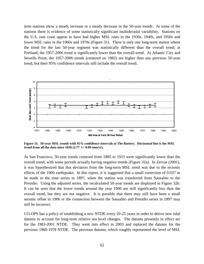
62

term stations show a steady increase or a steady decrease in the 50-year trends. At some of the

stations there is evidence of some statistically significant multidecadal variability. Stations on

the U.S. east coast appear to have had higher MSL rates in the 1930s, 1940s, and 1950s and

lower MSL rates in the 1960s and 1970s (Figure 31). There is only one long-term station where

the trend for the last 50-year segment was statistically different than the overall trend; at

Portland, the 1957-2006 trend is significantly lower than the overall trend. At Atlantic City and

Sewells Point, the 1957-2006 trends (centered on 1982) are higher than any previous 50-year

trend, but their 95% confidence intervals still include the overall trend.

Figure 31. 50-year MSL trends with 95% confidence intervals at The Battery. Horizontal line is the MSL

trend from all the data since 1856 (2.77 +/- 0.09 mm/yr).

At San Francisco, 50-year trends centered from 1885 to 1915 were significantly lower than the

overall trend, with some periods actually having negative trends (Figure 32a). In Zervas (2001),

it was hypothesized that this deviation from the long-term MSL trend was due to the tectonic

effects of the 1906 earthquake. In this report, it is suggested that a small correction of 0.037 m

be made to the time series in 1897, when the station was transferred from Sausalito to the

Presidio. Using the adjusted series, the recalculated 50-year trends are displayed in Figure 32b.

It can be seen that the lower trends around the year 1900 are still significantly less than the

overall trend, but they are not negative. It is possible that there may still have been a small

seismic offset in 1906 or the connection between the Sausalito and Presidio series in 1897 may

still be incorrect.

CO-OPS has a policy of establishing a new NTDE every 20-25 years in order to derive new tidal

datums to account for long-term relative sea level changes. The datums presently in effect are

for the 1983-2001 NTDE. They went into effect in 2003 and replaced the datums for the

previous 1960-1978 NTDE. The previous datums, which roughly represented the level of MSL

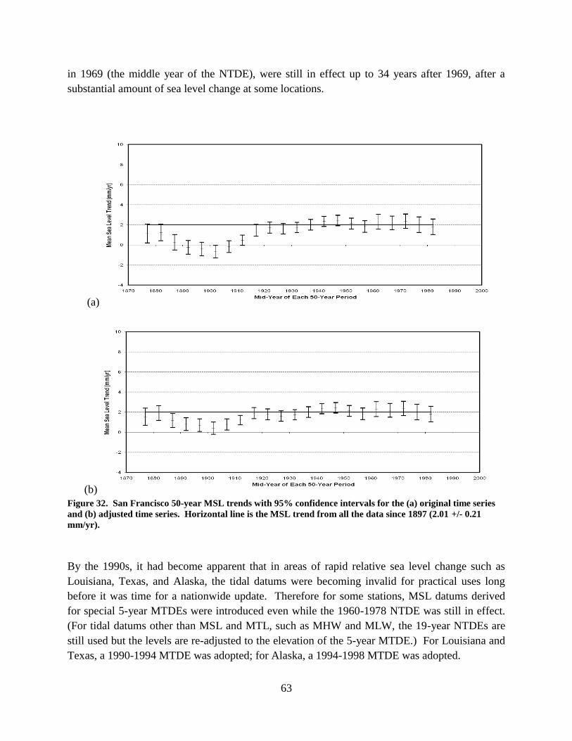
63

in 1969 (the middle year of the NTDE), were still in effect up to 34 years after 1969, after a

substantial amount of sea level change at some locations.

(a)

(b)

Figure 32. San Francisco 50-year MSL trends with 95% confidence intervals for the (a) original time series

and (b) adjusted time series. Horizontal line is the MSL trend from all the data since 1897 (2.01 +/- 0.21

mm/yr).

By the 1990s, it had become apparent that in areas of rapid relative sea level change such as

Louisiana, Texas, and Alaska, the tidal datums were becoming invalid for practical uses long

before it was time for a nationwide update. Therefore for some stations, MSL datums derived

for special 5-year MTDEs were introduced even while the 1960-1978 NTDE was still in effect.

(For tidal datums other than MSL and MTL, such as MHW and MLW, the 19-year NTDEs are

still used but the levels are re-adjusted to the elevation of the 5-year MTDE.) For Louisiana and

Texas, a 1990-1994 MTDE was adopted; for Alaska, a 1994-1998 MTDE was adopted.

64

When the 1983-2001 NTDE was introduced, the regions with trends greater than 6 mm/yr were

given MSL datums representing only the last 5 years of the new epoch (1997-2001). It was

expected that these stations would require updates every 5 years because they would have

changed by at least 0.030 m. When the 2002-2006 period was analyzed, due to the effects of

interannual variability on the long-term trend, some of these stations had changed by less than

0.030 m while some other stations with smaller trends had changed by over 0.030 m.

Since CO-OPS will continue to use 5-year periods as an option to update datums in regions of

rapid sea level change, a rule should be established for when to change to a new 5-year datum. It

would be advantageous not to change the datums more often than necessary. It should also be

kept in mind that if global sea level rise should accelerate in the future, more frequent updates

would be required at many more stations.

For all the stations that have not been selected for a 5-year datum, Figure 33 shows the mean sea

level for 2002-2006 relative to the 1983-2001 MSL datum still in effect. This 5-year period is

centered on 2004 and represents roughly 12 years of MSL change since 1992. The values in

Figure 33 are also affected by interannual variations and any small multidecadal changes in

trend. Although some stations have changed little, many others have changed by more than

0.030 m. Therefore, not all currently accepted MSL datums reflect present-day MSL.

The next two 5-year datum periods will be 2007-2011 and 2012-2016, which will correspond to

17 years and 22 years after 1992, the center year of the current NTDE. CO-OPS will evaluate

the changes in MSL and decide which stations will require a datum update in advance of the next

nationwide update due sometime after 2020. Given current sea level trends, it is likely that most

stations will be even further from the established NTDE datum than the values in Figure 33. If

too many stations were to be switched to a 5-year datum to make them accurate to 0.030 m, the

concept of a NTDE becomes obsolete. Therefore, the 0.030 m threshold may be too narrow of a

tolerance in practice.

The absolute amounts of MSL change that can be expected 12 and 22 years after the center year

of the NTDE, due solely to the relative MSL trends in Table 4, are plotted in Figure 34. If 0.l00

m were selected as the threshold for requiring a datum update, after 12 years (2002-2006) only

the stations with trends above 8 mm/yr would likely require a new datum. After 22 years (2012-

2016), only the stations with trends above 4.5 mm/yr would be likely to require a new datum

when using a 0.100 m threshold.

All of the stations with trends above 6 mm/yr plus Freeport, Rockport, Anchorage, and Unalaska

are already on a 5-year datum. Therefore, it is suggested that 0.100 m be adopted as a threshold

for a 5-year datum update. When the MSL for a 5-year period is compared to the NTDE datum

or to a previous 5-year MSL datum and the change is greater than 0.100 m, a new datum should

be adopted. Because 19 out of 128 stations have trends above 4.5 mm/yr, only 15% of the long-

term stations would have 5-year datums before a nationwide update is due. With a 0.100 m

65

threshold for a datum update, only Skagway, the station with the greatest rate, will need to be

updated every 5 years. The other stations with trends above 4.5 mm/yr will be able to remain on

the same MSL datum for periods of 10 or even 15 years before requiring an update.

Figure 33. Mean sea level for 2002-2006 relative to the 1983-2001 MSL datum for stations that have not been

updated to a 5-year MSL datum due to rapid relative sea level trends.

66

Figure 34. Estimated absolute MSL change for 12 and 22 years after the establishment of an NTDE as a

function of the rate of sea level change.

67

CONCLUSION

This report is a re-analysis of mean sea level variations in the United States using monthly MSL

data from long-term NWLON stations with a data range of at least 30 years. The report follows

the format of Zervas (2001) with seven additional years of data and presents results for 12

additional stations. A total of 128 stations were analyzed for linear trends, autoregressive

coefficients, average seasonal cycles, and interannual variability along with their 95%

confidence intervals. The stations are located on the U.S. east and west coasts, the Gulf of

Mexico, Alaska, Hawaii, Bermuda, the Caribbean, and on islands in the Pacific Ocean (Figures

1-7, Appendix I). The two oldest stations, The Battery and San Francisco, have records

beginning in the 1850s. The maintenance of these long-term time series depends on the

continued monitoring of tidal bench marks. The reference elevations of the station datums have

been preserved despite the occasionally-required relocations of some of the stations.

Linear MSL trends were calculated using linear regression with an autoregressive coefficient of

order 1 in order to obtain accurate error estimates. This method was used because of the serial

correlation of the residual time series due to interannual variability caused by the effects of

ENSO and other driving forces on coastal oceanic water temperatures, salinities, winds, air

pressures, and currents. The linear trends range from 9.65 mm/yr at Eugene Island to -17.12 at

Skagway (Table 4, Figures 9-11). The calculated trends are relative trends which are comprised

of the absolute change in the level of the ocean and the vertical motion of the land. The global

rate of sea level rise in the 20th

century was 1.7 +/- 0.5 mm/yr (Solomon 2007). Although there

were probably some smaller regional multidecadal variations in absolute sea level trends, most of

the variation in relative sea level trends from station to station is due to local vertical land motions.

Time series plots for each station of the monthly MSL data with the average seasonal cycle

removed are shown in Appendix II. The times of any major earthquakes in the vicinity are noted

on the plots as a solid vertical line, because a seismic offset and/or a change in trend are possible.

Separate pre-seismic and post-seismic trends were calculated at Guam, Yakutat, Cordova, Seward,

Kodiak Island, Adak Island, and Unalaska due to observed seismic offsets in 1957, 1964, or 1993.

Post-seismic trends usually indicate more rapid vertical land motion than pre-seismic trends.

The average seasonal cycles represented by twelve monthly values are plotted in Appendix III

for each station, indicating the regular, repeatable variation in water levels over the course of a

year. This variation is incorporated into the CO-OPS tidal predictions via two tidal constituents,

Sa and Ssa. The twelve monthly values for each station’s average seasonal cycle are used to

derive values for Sa and Ssa which are listed in Appendix IV and compared to the accepted CO-

OPS tidal constituents used for the official tide tables.

When the linear trend and the average seasonal cycle are removed from the monthly MSLs, the

residual time series, representing regional oceanic interannual variability, are highly correlated

from station to station. A 5-month running average of the residual time series is used to define

68

times of unusually high or low water levels. When the 5-month running average is above 0.1 m

or below -0.1 m, a positive or negative anomaly is defined. A table of the number of months

with positive or negative anomalies each year (Tables 6 and 7), shows the timing and regional

extent of anomalous water levels along a coastline. The major driver of anomalies on the U.S.

west coast and in the western Pacific Ocean is ENSO variability. East coast and Gulf coast

anomalies appear to be caused by multiple driving forces without any single dominant forcing.

Each derived linear trend has an associated uncertainty represented by error bars showing the 95%

confidence interval. The 95% confidence intervals of the MSL trends can be related to the year

range of data by an inverse power relationship. This empirically-derived relationship indicates

how poorly-defined a linear trend derived from only 20 years of data can be. In contrast, a trend

derived from 50-60 years of data is more precisely defined since it is much less affected by the

interannual variability found in MSL time series. In general, for a given length of data, error bars

are wider for Pacific Ocean and western Gulf of Mexico stations than for Atlantic Ocean and

eastern Gulf of Mexico stations due to the different amplitudes of interannual variability.

Since trends derived from 50 years of MSL data have relatively small error bars, a long-term

time series can be divided up into 50-year segments and an examination of their trends and

associated confidence intervals can determine whether there is a statistically significant

multidecadal variation in the time series. The 25 stations with the longest time series (over 80

years of data) have been divided into series of 50-year segments each offset by 5 years to

determine how the MSL trends change over time. Most stations showed no long-term increase

or decrease in the 50-year trends, but some Atlantic coast stations had statistically significant

multidecadal variability with slightly higher trends in the 1930s, 1940s, and 1950s and slightly

lower trends in the 1960s and 1970s. The greatest multidecadal variability was found in the

longest NWLON series at San Francisco, where 50-year trends centered near the year 1900 were

actually negative. A re-examination of the history of the San Francisco time series, which was

put together with data from 3 separate locations, indicated the possibility of an error in the

connection between the Sausalito and the Presidio series occurring in 1897. When the time

series is adjusted and the 50-year trends are recalculated, the 50-year trends around 1900 are still

significantly lower than the overall trend but they are not negative.

One of the consequences of changing sea levels is that most datums defined by CO-OPS become

obsolete after several decades. The concept of a 19-year NTDE, introduced to define a MSL

datum for a specific time period, requires a nationwide change to a new NTDE after 20-25 years

when a sufficient amount of sea level change has taken place at most stations. In some regions,

extremely rapid rates of relative sea level change required the introduction of special 5-year MSL

datums. Some NWLON stations are currently on a 1997-2001 MTDE and some are on a 2002-

2006 MTDE. Furthermore, some of the stations on the 1983-2001 NTDE are gradually drifting

away from their established MSL datum. In this report, it is proposed that a new datum be

introduced when MSL at a station, calculated over a 5-year period, has changed by over 0.100 m

69

from its previously established datum. If this rule is adopted, only about 15% of the NWLON

stations with the highest MSL trends would be on 5-year datums after 20-25 years, when a new

NTDE can be established.

Eight NWLON stations now have data spanning periods of over 100 years. These stations are

The Battery, Philadelphia, Baltimore, Fernandina Beach, San Diego, San Francisco, Seattle, and

Honolulu. Figure 35 graphically summarizes these CO-OPS data sets and demonstrates the

value of continuous, long-term sea level measurements. Together, these series represent the

effect of globally-rising sea levels on most of the U.S. coastline. Although there is a small

amount of subsidence at The Battery, Philadelphia, and Baltimore (about 1 mm/yr), the other

five stations have negligible vertical land motion and therefore have been recording the absolute

global 20th

century sea level rise of 1.7 mm/yr (Douglas, 1991). As shown in Figure 35, the

importance of the demonstrated global sea level rise derived from the long-term sea level

observations is analogous to the importance of the atmospheric CO2 observations to the global

climate system.

Figure 35. Comparison of the atmospheric carbon dioxide record at Mauna Loa, Hawaii since 1958 (from

http://www.esrl.noaa.gov/gmd/ccgg/trends/co2_data_mlo.html ) and monthly mean sea levels at eight

NWLON stations with record lengths of over 100 years.

70

71

ACKNOWLEDGMENTS

The high quality of the United States sea level database is a result of the sustained operation and

maintenance of a nationwide water level observation network since the 1850s and the processing,

analysis, and archiving of the data accomplished by the efforts of numerous employees of the

Center for Operational Oceanic Products and Services and its predecessor agencies. The

extraction of the data set used for this analysis was assisted by Tom Huppmann. This report was

reviewed by Stephen Gill, William Sweet, Kathleen Egan, and John Boon who provided many

useful suggestions for improving the document. This report was prepared for publication by

Brenda Via.

72

73

REFERENCES

Baringer, M. O. & J. C. Larsen (2001) Sixteen years of Florida Current transport at 27 degrees

N. Geophysical Research Letters, 28, 3179-3182.

Blaha, J. P. (1984) Fluctuations of monthly sea-level as related to the intensity of the Gulf-

Stream from Key West to Norfolk. Journal of Geophysical Research-Oceans, 89, 8033-

8042.

Burgette, R. J., R. J. Weldon & D. A. Schmidt (2009) Interseismic uplift rates for western

Oregon and along-strike variation in locking on the Cascadia subduction zone. Journal of

Geophysical Research-Solid Earth, 114, 24.

Cazenave, A. & R. S. Nerem (2004) Present-day sea level change: Observations and causes.

Reviews of Geophysics, 42.

Center for Operational Oceanographic Products and Services. 1999. Tide and current glossary.

[Silver Spring, Md.: U.S. Dept. of Commerce, National Oceanic and Atmospheric

Administration, National Ocean Service, Center for Operational Oceanographic Products

and Services.

Church, J. A. & N. J. White (2006) A 20th century acceleration in global sea-level rise.

Geophysical Research Letters, 33.

Church, J. A., N. J. White, R. Coleman, K. Lambeck & J. X. Mitrovica (2004) Estimates of the

regional distribution of sea level rise over the 1950-2000 period. Journal of Climate, 17,

2609-2625.

Climate Prediction Center. 1999. Climate Prediction Center (CPC) : El Niño and La Niña

advisories, climate outlooks and data, and stratospheric ozone. U.S. Dept. of Commerce,

National Oceanic and Atmospheric Administration, National Weather Service, National

Center for Environmental Prediction, Climate Prediction Center.

http://www.cpc.ncep.noaa.gov/index.php (last accessed.

Cohen, S. C. & J. T. Freymueller (2001) Crustal uplift in the south central Alaska subduction

zone: New analysis and interpretation of tide gauge observations. Journal of Geophysical

Research-Solid Earth, 106, 11259-11270.

Davis, J. L. & J. X. Mitrovica (1996) Glacial isostatic adjustment and the anomalous tide gauge

record of eastern North America. Nature, 379, 331-333.

Dokka, R. K., G. F. Sella & T. H. Dixon (2006) Tectonic control of subsidence and southward

displacement of southeast Louisiana with respect to stable North America. Geophysical

Research Letters, 33.

Douglas, B. C. (1991) Global sea-level rise. Journal of Geophysical Research-Oceans, 96, 6981-

6992.

--- (1992) Global sea-level acceleration. Journal of Geophysical Research-Oceans, 97, 12699-

12706.

--- (1997) Global sea rise: A redetermination. Surveys in Geophysics, 18, 279-292.

Gill, S. K. & J. R. Schultz. 2001. Tidal datums and their applications. Silver Spring, MD:

National Oceanic and Atmospheric Administration.

74

Hicks, S. D. & J. E. Crosby. 1974. Trends and variability of yearly mean sea-level, 1893-1972.

Rockville, Md.: U.S. Dept. of Commerce, National Oceanic and Atmospheric

Administration, National Ocean Survey.

Hicks, S. D., H. A. Debaugh & L. E. Hickman. 1983. Sea level variations for the United States,

1855-1980. Rockville, Md.: U.S. Dept. of Commerce, National Oceanic and Atmospheric

Administration, National Ocean Service.

Hicks, S. D. & W. Shofnos (1965) Yearly sea level variations for the United States. Journal

Name: J. Hydraul. Div., Am. Soc. Civ. Eng.; (United States); Journal Volume: 5:4468,

Medium: X; Size: Pages: 23-32.

Holgate, S. J. (2007) On the decadal rates of sea level change during the twentieth century.

Geophysical Research Letters, 34.

Holgate, S. J. & P. L. Woodworth (2004) Evidence for enhanced coastal sea level rise during the

1990s. Geophysical Research Letters, 31.

Ivins, E. R., R. K. Dokka & R. G. Blom (2007) Post-glacial sediment load and subsidence in

coastal Louisiana. Geophysical Research Letters, 34.

Jevrejeva, S., A. Grinsted, J. C. Moore & S. Holgate (2006) Nonlinear trends and multiyear

cycles in sea level records. Journal of Geophysical Research-Oceans, 111, 11.

Jevrejeva, S., J. C. Moore, A. Grinsted & P. L. Woodworth (2008) Recent global sea level

acceleration started over 200 years ago? Geophysical Research Letters, 35.

Larsen, C. F., K. A. Echelmeyer, J. T. Freymueller & R. J. Motyka (2003) Tide gauge records of

uplift along the northern Pacific-North American plate boundary, 1937 to 2001. Journal

of Geophysical Research-Solid Earth, 108.

Larsen, C. F., R. J. Motyka, J. T. Freymueller, K. A. Echelmeyer & E. R. Ivins (2004) Rapid

uplift of southern Alaska caused by recent ice loss. Geophysical Journal International,

158, 1118-1133.

--- (2005) Rapid viscoelastic uplift in southeast Alaska caused by post-Little Ice Age glacial

retreat. Earth and Planetary Science Letters, 237, 548-560.

Lawson, A. C. & H. F. Reid. 1908. The California earthquake of April 18, 1906 : report of the

State Earthquake Investigation Commission in two volumes and atlas. Washington, D.C.:

Carnegie Institution of Washington.

Lyles, S. D., L. E. Hickman & H. A. Debaugh. 1988. Sea level variations for the United States,

1855-1986. [Rockville, Md.]: U.S. Dept. of Commerce, National Oceanic and

Atmospheric Administration, National Ocean Service, Office of Oceanography and

Marine Assessment.

Nerem, R. S., E. Leuliette & A. Cazenave (2006) Present-day sea-level change: A review.

Comptes Rendus Geoscience, 338, 1077-1083.

Noble, M. A. & G. R. Gelfenbaum (1992) Seasonal fluctuations in sea-level on the South-

Carolina shelf and their relationship to the Gulf-Stream. Journal of Geophysical

Research-Oceans, 97, 9521-9529.

75

Ryan, H. F. & M. A. Noble (2007) Sea level fluctuations in central California at subtidal to

decadal and longer time scales with implications for San Francisco Bay, California.

Estuarine Coastal and Shelf Science, 73, 538-550.

Sandeen, W. M. & J. B. Wesselman. 1973. Ground-Water Resources of Brazoria County, Texas.

Texas Water Development Board.

Schureman, P. 1958. Manual of harmonic analysis and prediction of tides. Washington:

Department of Commerce ; U.S. G.P.O.

Sella, G. F., S. Stein, T. H. Dixon, M. Craymer, T. S. James, S. Mazzotti & R. K. Dokka (2007)

Observation of glacial isostatic adjustment in "stable" North America with GPS.

Geophysical Research Letters, 34.

Smith, R. A. (1980) Golden Gate Tidal Measurements: 1854-1978. Journal of the Waterway

Port Coastal and Ocean Division, 106, 407-409.

---. 2002. Historical Golden Gate Tidal Series. In NOAA Technical Report NOS CO-OPS. Silver

Spring, MD: U.S. Department of Commerce, National Oceangraphic and Atmospheric

Administration, National Ocean Service.

Solomon, S. 2007. Climate change 2007 : the physical science basis : contribution of Working

Group I to the Fourth Assessment Report of the Intergovernmental Panel on Climate

Change. Cambridge ; New York: Cambridge University Press.

Storch, H. v. & F. W. Zwiers. 2001. Statistical analysis in climate research. Cambridge, UK ;

New York: Cambridge University Press.

White, N. J., J. A. Church & J. M. Gregory (2005) Coastal and global averaged sea level rise for

1950 to 2000. Geophysical Research Letters, 32.

Wilks, D. S. 2006. Statistical methods in the atmospheric sciences. Burlington, Mass.: Academic

Press.

Woodworth, P. L. (1990) A search for accelerations in records of European mean sea-level.

International Journal of Climatology, 10, 129-143.

Woodworth, P. L., N. J. White, S. Jevrejeva, S. J. Holgate, J. A. Church & W. R. Gehrels (2009)

Evidence for the accelerations of sea level on multi-decade and century timescales.

International Journal of Climatology, 29, 777-789.

Zervas, C. E. 1999. Tidal Current Analysis Procedures and Associated Computer Programs.

Silver Spring, Md.: U.S. Dept. of Commerce, National Oceanic and Atmospheric

Administration, National Ocean Service.

---. 2001. Sea level variations of the United States, 1854-1999. Silver Spring, Md.: U.S. Dept. of

Commerce, National Oceanic and Atmospheric Administration, National Ocean Service.

76

77

APPENDICES

APPENDIX I

National Water Level Observation Network Stations

APPENDIX II

Time series of monthly mean sea level after removal of the average seasonal cycle showing

the derived linear trend

APPENDIX III

Average seasonal cycle of monthly mean sea level with 95% confidence intervals

APPENDIX IV

Comparison of Sa and Ssa tidal constituents derived from average seasonal cycles with the

accepted tidal constituents used for CO-OPS tide predictions

APPENDIX V

Linear trends for 50-year periods of mean sea level data

78

 

A-1

 

 

 

 

Appendix I.

National Water Level Observation Network Stations  

 

 

 

 

 

 

 

 

 

 

 

 

 

 

 

 

 

 

 

A-2

 

Table A. NWLON Stations

Station Number

Latitude Longitude First Year

Last Year

Year Range

Station Name State or Territory

1611400 21.955 -159.357 1955 2006 52 Nawiliwili Hawaii

1612340 21.307 -157.867 1905 2006 102 Honolulu Hawaii

1612480 21.437 -157.793 1957 2006 50 Mokuoloe Hawaii

1615680 20.898 -156.472 1947 2006 60 Kahului Hawaii

1617760 19.73 -155.057 1927 2006 80 Hilo Hawaii

1619000 16.738 -169.53 1947 2003 57 Johnston Atoll

1619910 28.212 -177.36 1947 2006 60 Midway Atoll

1630000 13.442 144.653 1948 1993 46 Guam Marianas Is.

1770000 -14.28 -170.69 1948 2006 59 Pago Pago American Samoa

1820000 8.737 167.738 1946 2006 61 Kwajalein Marshall Is.

1840000 7.447 151.847 1947 1995 49 Chuuk Caroline Is.

1890000 19.29 166.618 1950 2006 57 Wake Island

2695535 2695540

32.373 -64.703 1932 2006 75 Bermuda

8410140 44.903 -66.985 1929 2006 78 Eastport Maine

8413320 44.392 -68.205 1947 2006 60 Bar Harbor Maine

8418150 43.657 -70.247 1912 2006 95 Portland Maine

8419870 43.08 -70.742 1926 2001 76 Seavey Island Maine

8443970 42.355 -71.052 1921 2006 86 Boston Massachusetts

8447930 41.523 -70.672 1932 2006 75 Woods Hole Massachusetts

8449130 41.285 -70.097 1965 2006 42 Nantucket Island Massachusetts

8452660 41.505 -71.327 1930 2006 77 Newport Rhode Island

8454000 41.807 -71.402 1938 2006 69 Providence Rhode Island

8461490 41.355 -72.087 1938 2006 69 New London Connecticut

8467150 41.173 -73.182 1964 2006 43 Bridgeport Connecticut

8510560 41.048 -71.96 1947 2006 60 Montauk New York

8514560 40.95 -73.077 1957 1992 36 Port Jefferson New York

8516990 8516945

40.81 -73.765 1931 2006 76 Willets Point / Kings Point New York

8518750 40.7 -74.015 1856 2006 151 The Battery New York

8531680 40.467 -74.01 1932 2006 75 Sandy Hook New Jersey

8534720 39.355 -74.418 1911 2006 96 Atlantic City New Jersey

8536110 38.968 -74.96 1965 2006 42 Cape May New Jersey

8505530 8545240

39.933 -75.142 1900 2006 107 Philadelphia Pennsylvania

8551910 39.558 -75.573 1956 2006 51 Reedy Point Delaware

8557380 38.782 -75.12 1919 2006 88 Lewes Delaware

8570280 8570283

38.328 -75.092 1975 2006 32 Ocean City Maryland

8571890 8571892

38.573 -76.068 1943 2006 64 Cambridge Maryland

8573927 39.527 -75.81 1972 2006 35 Chesapeake City Maryland

8574680 39.267 -76.578 1902 2006 105 Baltimore Maryland

8575512 38.983 -76.48 1928 2006 79 Annapolis Maryland

8577330 38.317 -76.452 1937 2006 70 Solomons Island Maryland

8594900 38.873 -77.022 1924 2006 83 Washington D. C.

 

A-3

 

Table A. NWLON Stations

Station Number

Latitude Longitude First Year

Last Year

Year Range

Station Name State or Territory

8632200 37.167 -75.988 1951 2006 56 Kiptopeke Virginia

8635150 38.252 -76.96 1972 2003 32 Colonial Beach Virginia

8635750 37.995 -76.465 1974 2006 33 Lewisetta Virginia

8637624 37.247 -76.5 1950 2003 54 Gloucester Point Virginia

8638610 36.947 -76.33 1927 2006 80 Sewells Point Virginia

8638660 36.822 -76.293 1935 1987 53 Portsmouth Virginia

8638863 36.967 -76.113 1975 2006 32 Chesapeake Bay Bridge Tunnel Virginia

8652587 35.795 -75.548 1977 2006 30 Oregon Inlet Marina North Carolina

8656495 8656483

34.72 -76.67 1953 2006 54 Beaufort North Carolina

8658120 34.227 -77.953 1935 2006 72 Wilmington North Carolina

8659084 33.915 -78.018 1933 2006 74 Southport North Carolina

8661000 8661070

33.655 -78.918 1957 2006 50 Springmaid Pier South Carolina

8665530 32.782 -79.925 1921 2006 86 Charleston South Carolina

8670870 32.033 -80.902 1935 2006 72 Fort Pulaski Georgia

8720030 30.672 -81.465 1897 2006 110 Fernandina Beach Florida

8720220 8720218

30.397 -81.43 1928 2006 79 Mayport Florida

8721020 8721120

29.147 -80.963 1925 1983 59 Daytona Beach Shores Florida

8723170 25.768 -80.132 1931 1981 51 Miami Beach Florida

8723970 24.712 -81.105 1971 2006 36 Vaca Key Florida

8724580 24.553 -81.808 1913 2006 94 Key West Florida

8725110 26.13 -81.807 1965 2006 42 Naples Florida

8725520 26.647 -81.872 1965 2006 42 Fort Myers Florida

8726520 27.76 -82.627 1947 2006 60 St. Petersburg Florida

8726724 27.978 -82.832 1973 2006 34 Clearwater Beach Florida

8727520 29.135 -83.032 1914 2006 93 Cedar Key Florida

8728690 29.727 -84.982 1967 2006 40 Apalachicola Florida

8729108 30.152 -85.667 1973 2006 34 Panama City Florida

8729840 30.403 -87.212 1923 2006 84 Pensacola Florida

8735180 30.25 -88.075 1966 2006 41 Dauphin Island Alabama

8761720 8761724

29.263 -89.957 1947 2006 60 Grand Isle Louisiana

8764311 29.372 -91.385 1939 1974 36 Eugene Island Louisiana

8770590 8770570

29.73 -93.87 1958 2006 49 Sabine Pass Texas

8771450 29.31 -94.793 1908 2006 99 Galveston Pier 21 Texas

8771510 29.285 -94.788 1957 2006 50 Galveston Pleasure Pier Texas

8772440 28.948 -95.308 1954 2006 53 Freeport Texas

8774770 28.022 -97.047 1948 2006 59 Rockport Texas

8778490 26.565 -97.43 1963 2006 44 Port Mansfield Texas

8779750 26.068 -97.152 1958 2006 49 Padre Island Texas

8779770 26.06 -97.215 1944 2006 63 Port Isabel Texas

9410170 32.713 -117.173 1906 2006 101 San Diego California

9410230 32.867 -117.258 1924 2006 83 La Jolla California

 

A-4

 

Table A. NWLON Stations

Station Number

Latitude Longitude First Year

Last Year

Year Range

Station Name State or Territory

9410580 33.603 -117.883 1955 1993 39 Newport Beach California

9410660 33.72 -118.272 1923 2006 84 Los Angeles California

9410840 34.008 -118.5 1933 2006 74 Santa Monica California

9411270 34.348 -119.443 1962 1990 29 Rincon Island California

9411340 34.408 -119.685 1973 2006 34 Santa Barbara California

9412110 35.177 -120.76 1945 2006 62 Port San Luis California

9413450 36.605 -121.888 1973 2006 34 Monterey California

9414290 37.807 -122.465 1897 2006 110 San Francisco California

9414523 37.507 -122.21 1974 2006 33 Redwood City California

9414750 37.772 -122.298 1939 2006 68 Alameda California

9415020 37.997 -122.975 1975 2006 32 Point Reyes California

9415144 38.057 -122.038 1976 2006 31 Port Chicago California

9418767 40.767 -124.217 1977 2006 30 North Spit California

9419750 41.745 -124.183 1933 2006 74 Crescent City California

9431647 42.74 -124.497 1977 2006 30 Port Orford Oregon

9432780 43.345 -124.322 1970 2006 37 Charleston Oregon

9435380 44.625 -124.043 1967 2006 40 South Beach Oregon

9437540 45.555 -123.912 1970 2006 37 Garibaldi Oregon

9439040 46.208 -123.767 1925 2006 82 Astoria Oregon

9440910 46.708 -123.965 1973 2006 34 Toke Point Washington

9443090 48.368 -124.617 1934 2006 73 Neah Bay Washington

9444090 48.125 -123.44 1975 2006 32 Port Angeles Washington

9444900 48.112 -122.758 1972 2006 35 Port Townsend Washington

9447130 47.605 -122.338 1898 2006 109 Seattle Washington

9449424 48.863 -122.758 1973 2006 34 Cherry Point Washington

9449880 48.547 -123.01 1934 2006 73 Friday Harbor Washington

9450460 55.333 -131.625 1919 2006 88 Ketchikan Alaska

9451600 57.052 -135.342 1924 2006 83 Sitka Alaska

9452210 58.298 -134.412 1936 2006 71 Juneau Alaska

9452400 59.45 -135.327 1944 2006 63 Skagway Alaska

9453220 59.548 -139.735 1940 2006 67 Yakutat Alaska

9454050 60.558 -145.753 1964 2006 43 Cordova Alaska

9454240 61.125 -146.362 1973 2006 34 Valdez Alaska

9455090 60.12 -149.427 1964 2006 43 Seward Alaska

9455500 59.44 -151.72 1964 2006 43 Seldovia Alaska

9455760 60.683 -151.398 1973 2006 34 Nikiski Alaska

9455920 61.238 -149.89 1972 2006 35 Anchorage Alaska

9457292 9457283

57.732 -152.512 1975 2006 32 Kodiak Island Alaska

9459450 55.337 -160.502 1972 2006 35 Sand Point Alaska

9461380 51.863 -176.632 1957 2006 50 Adak Island Alaska

9462611 9462620

53.88 -166.537 1957 2006 50 Unalaska Alaska

9731158 19.907 -75.147 1937 1971 35 Guantanamo Bay Cuba

 

A-5

 

Table A. NWLON Stations

Station Number

Latitude Longitude First Year

Last Year

Year Range

Station Name State or Territory

9751401 17.697 -64.753 1977 2006 30 Lime Tree Bay Virgin Islands

9751639 18.335 -64.92 1975 2006 32 Charlotte Amalie Virgin Islands

9755371 18.458 -66.117 1962 2006 45 San Juan Puerto Rico

9759110 17.972 -67.047 1955 2006 52 Magueyes Island Puerto Rico

 

 

A-6

 

 

 

B-1

 

 

 

 

APPENDIX II

Time series of monthly mean sea level after removal of the average seasonal cycle

showing the derived linear trend  

 

 

 

 

 

 

 

 

 

 

 

 

 

Note: Dashed line indicates the monthly MSL and solid line indicates the 5‐month average.  Derived 

linear trends and 95% confidence intervals for the trends are also shown.  Vertical solid lines indicate 

times of major earthquakes.  Dashed vertical lines indicate beginning and end of periods of suspect data.  

The zero value on the vertical axis represents the elevation of the MSL datum for the National Tidal 

Datum Epoch (1983‐2001) or the special 5‐year Modified Tidal Datum Epoch, as appropriate. 

 

B-2

 

 

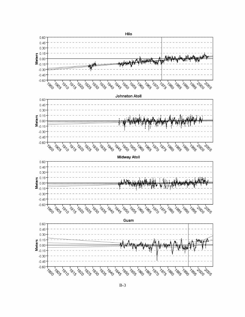
B-3

 

 

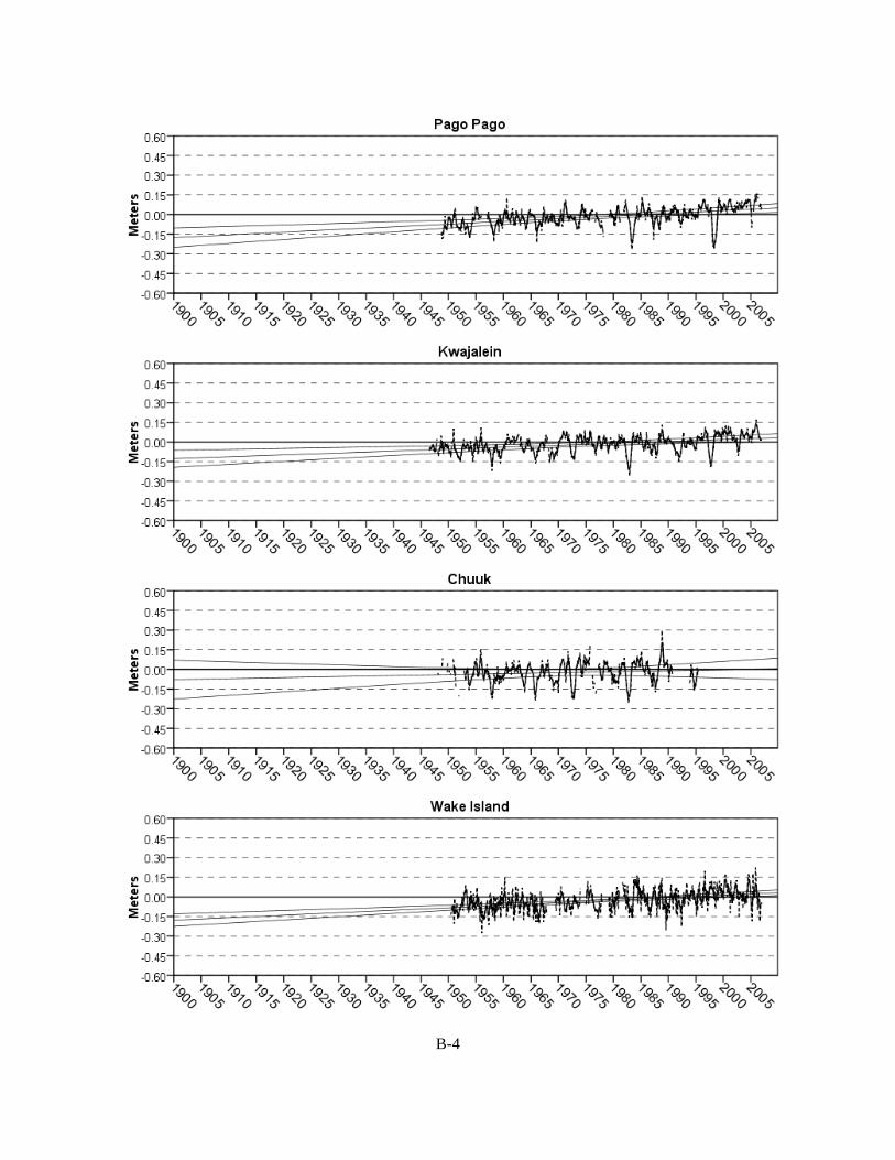
B-4

 

 

B-5

 

 

B-6

 

 

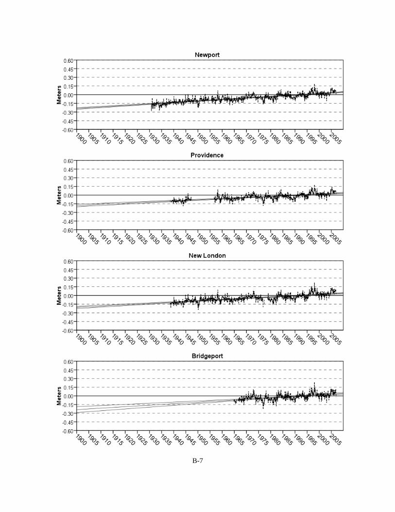
B-7

 

 

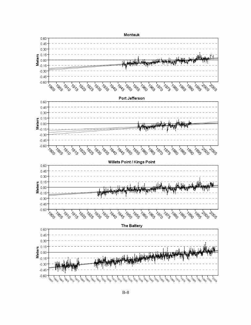
B-8

 

 

B-9

 

 

B-10

 

 

B-11

 

 

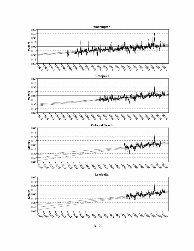
B-12

 

 

B-13

 

 

B-14

 

 

B-15

 

 

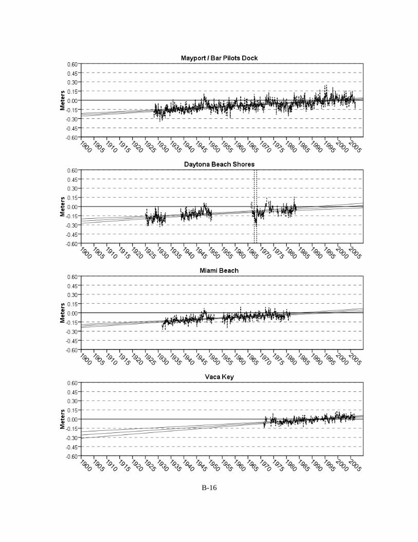
B-16

 

 

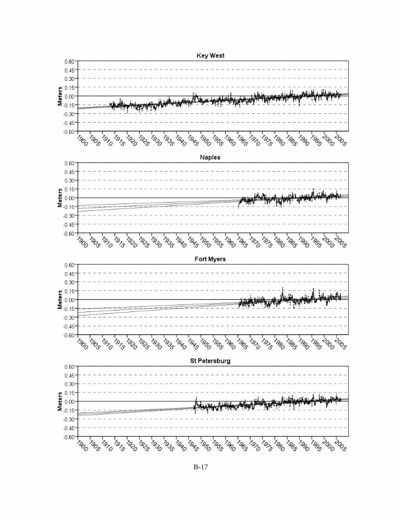
B-17

 

 

B-18

 

 

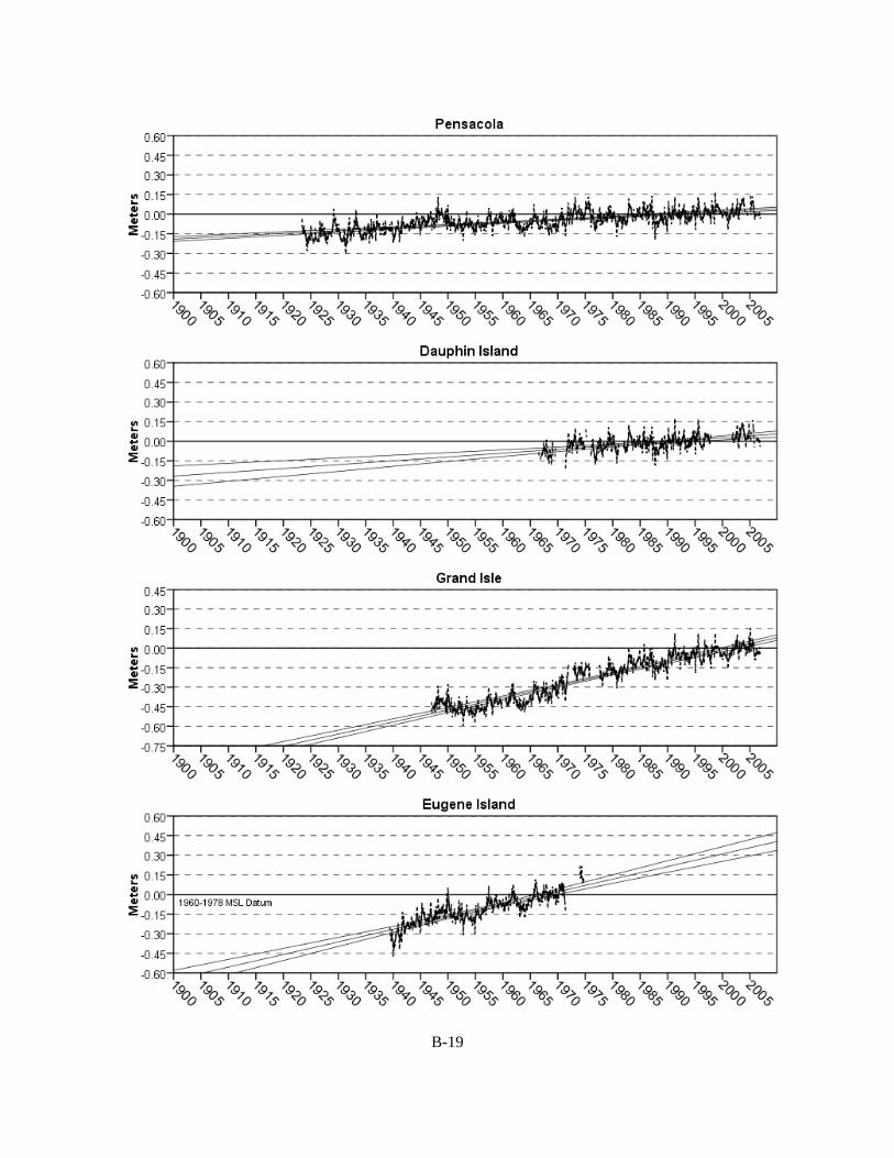
B-19

 

 

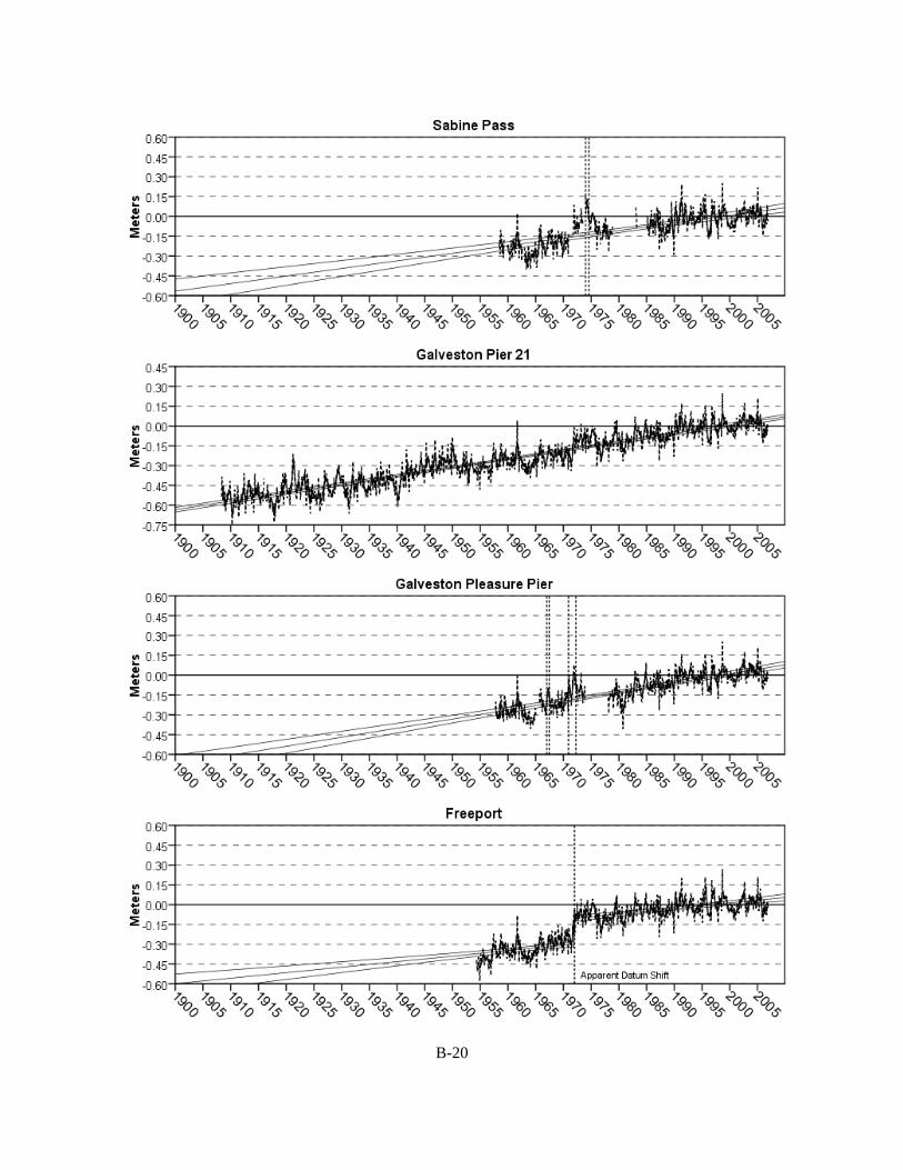
B-20

 

 

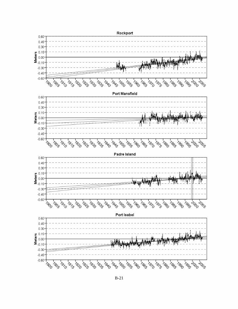
B-21

 

 

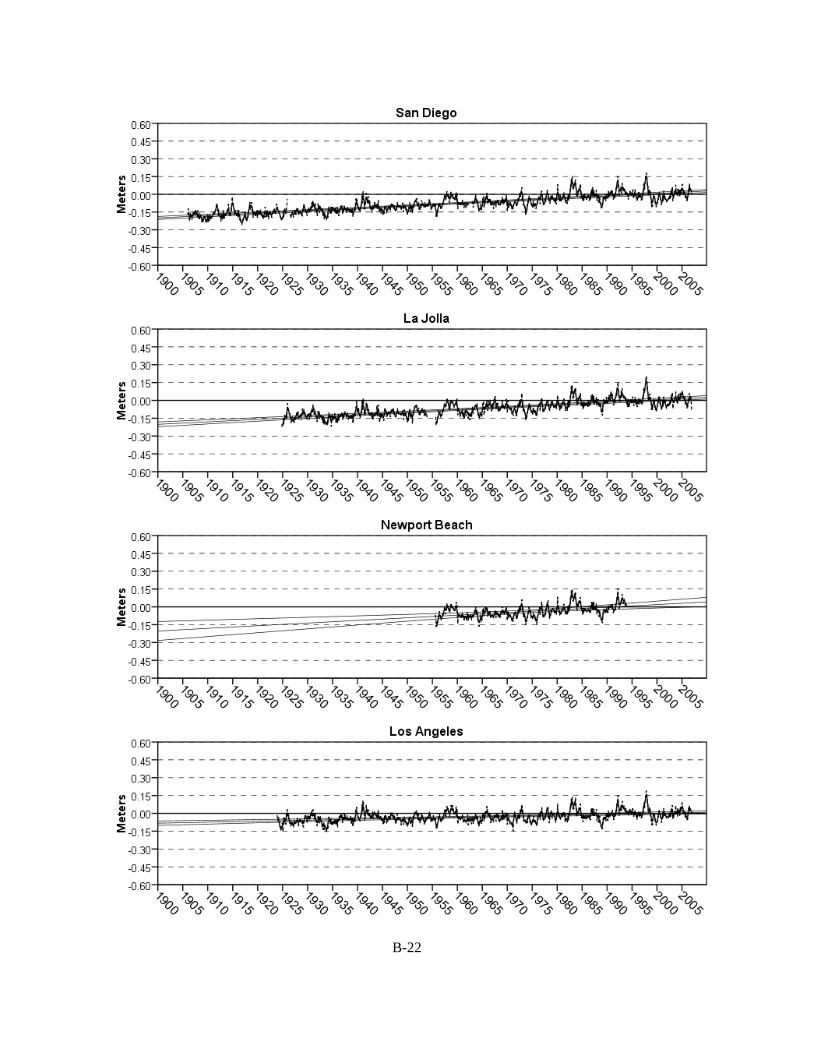
B-22

 

 

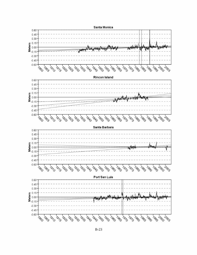
B-23

 

 

B-24

 

 

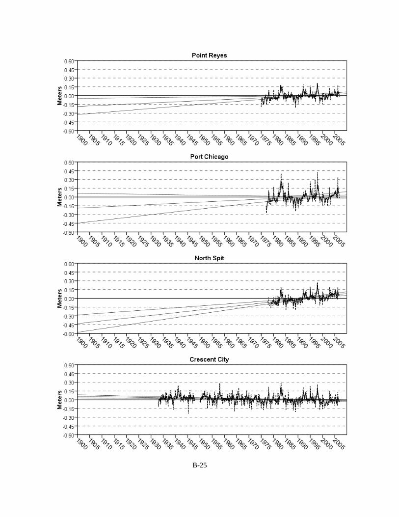
B-25

 

 

B-26

 

 

B-27

 

 

B-28

 

 

B-29

 

 

B-30

 

 

B-31

 

 

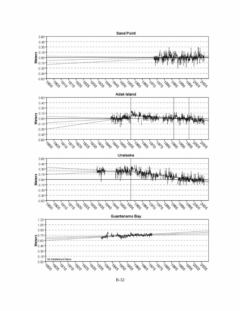
B-32

 

 

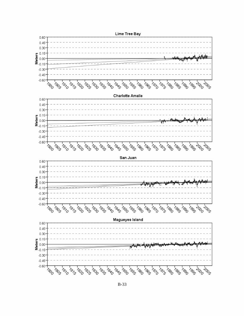
B-33

 

 

 

B-34

 

 

 

 

 

 

 

 

 

 

 

 

 

 

 

 

 

 

 

 

 

 

 

 

 

 

 

C-1

 

 

 

 

Appendix III

Average seasonal cycle

of monthly mean sea level

with 95% confidence intervals  

 

 

 

 

 

 

 

 

 

 

 

 

 

 

 

Note: The average of the monthly mean sea levels equals zero. 

 

C-2

 

 

Table B. Average seasonal mean sea level cycle (meters) Station  Jan  Feb  Mar  Apr May Jun Jul Aug Sep  Oct  Nov DecAdak Island  

0.079  0.060  ‐0.006  ‐0.065  ‐0.045  ‐0.045  ‐0.056  ‐0.040  ‐0.011  0.001  0.041  0.087 

Alameda  

0.028  0.030  ‐0.013  ‐0.061  ‐0.053  ‐0.021  0.009  0.021  0.040  0.014  ‐0.005  0.011 

Anchorage  

0.038  ‐0.027  ‐0.073  ‐0.093  ‐0.100  ‐0.054  0.004  0.039  0.069  0.074  0.056  0.068 

Annapolis  

‐0.124  ‐0.114  ‐0.063  ‐0.001  0.042  0.066  0.062  0.082  0.103  0.061  ‐0.012  ‐0.101 

Apalachicola  

‐0.106  ‐0.084  ‐0.026  ‐0.003  0.008  0.022  0.031  0.061  0.112  0.063  0.001  ‐0.079 

Astoria  

0.114  0.095  0.038  ‐0.015  ‐0.003  0.007  ‐0.081  ‐0.121  ‐0.112  ‐0.070  0.034  0.113 

Atlantic City  

‐0.077  ‐0.071  ‐0.046  ‐0.018  0.007  0.027  0.023  0.055  0.083  0.067  0.008  ‐0.059 

Baltimore  

‐0.134  ‐0.126  ‐0.073  ‐0.004  0.048  0.079  0.075  0.092  0.107  0.062  ‐0.021  ‐0.106 

Bar Harbor  

‐0.021  ‐0.024  ‐0.017  0.000  0.009  0.021  0.012  0.006  0.000  0.008  0.014  ‐0.009 

Beaufort  

‐0.075  ‐0.073  ‐0.054  ‐0.035  0.001  0.010  ‐0.009  0.030  0.104  0.114  0.033  ‐0.046 

Bermuda  

‐0.037  ‐0.046  ‐0.049  ‐0.061  ‐0.051  ‐0.022  0.011  0.045  0.070  0.087  0.049  0.003 

Boston  

‐0.041  ‐0.040  ‐0.022  0.001  0.015  0.027  0.014  0.014  0.016  0.022  0.016  ‐0.023 

Bridgeport  

‐0.087  ‐0.070  ‐0.045  ‐0.002  0.025  0.036  0.038  0.049  0.060  0.042  0.003  ‐0.051 

Cambridge  

‐0.109  ‐0.091  ‐0.056  ‐0.010  0.029  0.049  0.046  0.068  0.095  0.060  0.003  ‐0.084 

Cape May  

‐0.075  ‐0.065  ‐0.045  ‐0.007  0.012  0.018  0.016  0.042  0.083  0.062  0.008  ‐0.049 

Cedar Key  

‐0.115  ‐0.111  ‐0.066  ‐0.026  0.021  0.050  0.067  0.086  0.107  0.061  0.001  ‐0.076 

Charleston, OR 

0.114  0.097  0.038  ‐0.057  ‐0.089  ‐0.095  ‐0.082  ‐0.054  ‐0.028  ‐0.012  0.063  0.106 

Charleston, SC 

‐0.091  ‐0.080  ‐0.070  ‐0.046  0.006  0.013  ‐0.036  0.018  0.131  0.152  0.049  ‐0.044 

Charlotte Amalie 

‐0.035  ‐0.050  ‐0.050  ‐0.037  ‐0.035  ‐0.020  0.013  0.031  0.066  0.079  0.045  ‐0.007 

Cherry Point  

0.080  0.063  0.020  ‐0.055  ‐0.070  ‐0.051  ‐0.033  ‐0.021  ‐0.027  ‐0.023  0.048  0.070 

Ches Bay Brdg Tunnel 

‐0.081  ‐0.054  ‐0.037  ‐0.007  0.013  0.004  ‐0.007  0.034  0.099  0.082  0.009  ‐0.055 

Chesapeake City 

‐0.116  ‐0.098  ‐0.057  ‐0.016  0.055  0.073  0.054  0.065  0.103  0.050  ‐0.021  ‐0.093 

Chuuk  

‐0.054  ‐0.007  0.035  0.049  0.034  0.012  ‐0.002  ‐0.007  ‐0.002  0.011  ‐0.012  ‐0.056 

Clearwater Beach 

‐0.101  ‐0.096  ‐0.068  ‐0.032  0.013  0.031  0.039  0.059  0.111  0.077  0.031  ‐0.066 

Colonial Beach 

‐0.122  ‐0.094  ‐0.048  ‐0.001  0.048  0.053  0.046  0.075  0.107  0.052  ‐0.026  ‐0.090 

Cordova  

0.069  0.033  ‐0.027  ‐0.085  ‐0.117  ‐0.111  ‐0.098  ‐0.040  0.031  0.113  0.120  0.112 

Crescent City  

0.085  0.068  ‐0.001  ‐0.080  ‐0.087  ‐0.077  ‐0.037  ‐0.009  0.014  0.005  0.038  0.081 

Dauphin Island 

‐0.105  ‐0.098  ‐0.048  ‐0.004  0.025  0.022  0.000  0.045  0.126  0.086  0.018  ‐0.065 

 

C-3

 

Table B. Average seasonal mean sea level cycle (meters) Station  Jan  Feb  Mar  Apr May Jun Jul Aug Sep  Oct  Nov DecDaytona Bch Shores 

‐0.067  ‐0.060  ‐0.085  ‐0.066  ‐0.026  ‐0.019  ‐0.074  ‐0.029  0.130  0.187  0.109  0.000 

Eastport  

‐0.008  ‐0.014  ‐0.005  0.001  0.006  0.011  0.004  ‐0.009  ‐0.011  0.004  0.018  0.004 

Eugene Island 

‐0.119  ‐0.094  ‐0.040  0.031  0.062  0.055  ‐0.005  0.027  0.118  0.076  ‐0.019  ‐0.091 

Fernandina Beach 

‐0.091  ‐0.087  ‐0.081  ‐0.051  ‐0.004  ‐0.005  ‐0.073  ‐0.017  0.157  0.209  0.081  ‐0.038 

Fort Myers  

‐0.097  ‐0.097  ‐0.060  ‐0.034  ‐0.001  0.037  0.049  0.076  0.112  0.069  0.011  ‐0.065 

Fort Pulaski  

‐0.098  ‐0.094  ‐0.080  ‐0.047  0.012  0.013  ‐0.048  0.017  0.148  0.172  0.053  ‐0.049 

Freeport  

‐0.106  ‐0.095  ‐0.058  0.005  0.046  0.014  ‐0.060  ‐0.013  0.149  0.137  0.045  ‐0.065 

Friday Harbor 

0.089  0.070  0.021  ‐0.049  ‐0.069  ‐0.058  ‐0.047  ‐0.039  ‐0.037  ‐0.021  0.045  0.095 

Galveston Pier 21 

‐0.111  ‐0.095  ‐0.054  0.011  0.056  0.030  ‐0.047  ‐0.012  0.141  0.126  0.022  ‐0.068 

GalvPleasure Pier 

‐0.123  ‐0.101  ‐0.058  0.008  0.052  0.019  ‐0.047  0.000  0.153  0.134  0.032  ‐0.071 

Garibaldi  

0.147  0.118  0.070  ‐0.044  ‐0.104  ‐0.121  ‐0.129  ‐0.108  ‐0.064  ‐0.035  0.101  0.169 

Gloucester Point 

‐0.091  ‐0.074  ‐0.032  ‐0.010  0.021  0.021  0.000  0.046  0.100  0.083  0.004  ‐0.068 

Grand Isle  

‐0.106  ‐0.091  ‐0.053  ‐0.010  0.029  0.026  ‐0.008  0.036  0.137  0.097  0.013  ‐0.071 

Guam  

‐0.065  ‐0.034  ‐0.004  0.022  0.032  0.053  0.067  0.052  0.022  ‐0.018  ‐0.053  ‐0.073 

Guantanamo Bay 

‐0.047  ‐0.053  ‐0.043  ‐0.039  ‐0.019  ‐0.011  0.002  0.035  0.074  0.080  0.037  ‐0.017 

Hilo  

‐0.005  ‐0.022  ‐0.025  ‐0.035  ‐0.044  ‐0.036  ‐0.003  0.039  0.052  0.045  0.030  0.003 

Honolulu  

‐0.010  ‐0.019  ‐0.026  ‐0.037  ‐0.035  ‐0.024  0.003  0.030  0.049  0.043  0.026  0.003 

Johnston Atoll 

0.016  ‐0.020  ‐0.046  ‐0.055  ‐0.065  ‐0.058  ‐0.002  0.041  0.057  0.062  0.044  0.025 

Juneau  

0.028  ‐0.006  ‐0.045  ‐0.078  ‐0.083  ‐0.038  ‐0.036  ‐0.023  0.004  0.085  0.096  0.097 

Kahului  

‐0.005  ‐0.015  ‐0.025  ‐0.039  ‐0.043  ‐0.024  0.000  0.031  0.056  0.044  0.024  ‐0.004 

Ketchikan  

0.085  0.048  ‐0.010  ‐0.058  ‐0.087  ‐0.072  ‐0.085  ‐0.084  ‐0.045  0.061  0.119  0.128 

Key West  

‐0.062  ‐0.077  ‐0.069  ‐0.048  ‐0.020  ‐0.015  ‐0.011  0.029  0.091  0.127  0.072  ‐0.017 

Kings Point  

‐0.083  ‐0.078  ‐0.039  ‐0.002  0.022  0.039  0.038  0.053  0.065  0.047  0.004  ‐0.066 

Kiptopeke  

‐0.078  ‐0.065  ‐0.037  ‐0.019  0.008  0.013  0.000  0.039  0.096  0.085  0.017  ‐0.058 

Kodiak Island 

0.061  0.020  ‐0.032  ‐0.054  ‐0.079  ‐0.071  ‐0.066  ‐0.026  0.023  0.061  0.074  0.088 

Kwajalein  

‐0.057  ‐0.012  0.026  0.035  0.029  0.016  0.016  0.008  0.006  0.010  ‐0.023  ‐0.053 

La Jolla  

‐0.014  ‐0.037  ‐0.065  ‐0.078  ‐0.053  ‐0.015  0.036  0.063  0.079  0.050  0.025  0.009 

Lewes  

‐0.080  ‐0.062  ‐0.039  ‐0.011  0.016  0.022  0.013  0.040  0.079  0.067  0.010  ‐0.057 

Lewisetta  

‐0.109  ‐0.084  ‐0.053  ‐0.007  0.035  0.039  0.036  0.066  0.107  0.061  ‐0.012  ‐0.080 

 

C-4

 

Table B. Average seasonal mean sea level cycle (meters) Station  Jan  Feb  Mar  Apr May Jun Jul Aug Sep  Oct  Nov DecLime Tree Bay 

‐0.036  ‐0.052  ‐0.060  ‐0.047  ‐0.027  ‐0.013  0.015  0.035  0.068  0.075  0.047  ‐0.004 

Los Angeles  

‐0.010  ‐0.028  ‐0.061  ‐0.078  ‐0.053  ‐0.014  0.034  0.056  0.073  0.049  0.022  0.009 

Magueyes Island 

‐0.038  ‐0.048  ‐0.048  ‐0.046  ‐0.037  ‐0.019  0.019  0.041  0.061  0.075  0.048  ‐0.007 

Mayport  

‐0.078  ‐0.081  ‐0.083  ‐0.065  ‐0.024  ‐0.021  ‐0.075  ‐0.008  0.151  0.211  0.092  ‐0.020 

Miami Beach  

‐0.055  ‐0.067  ‐0.073  ‐0.057  ‐0.019  ‐0.023  ‐0.043  ‐0.005  0.083  0.164  0.100  ‐0.006 

Midway Atoll 

0.041  0.023  ‐0.022  ‐0.064  ‐0.056  ‐0.046  ‐0.029  0.024  0.050  0.030  0.022  0.028 

Mokuoloe  

‐0.005  ‐0.017  ‐0.024  ‐0.041  ‐0.044  ‐0.024  ‐0.001  0.027  0.049  0.042  0.031  0.005 

Montauk  

‐0.058  ‐0.055  ‐0.034  ‐0.016  0.005  0.021  0.029  0.037  0.048  0.041  0.016  ‐0.035 

Monterey  

0.015  0.005  ‐0.033  ‐0.073  ‐0.060  ‐0.032  0.013  0.035  0.062  0.039  0.017  0.013 

Nantucket Island 

‐0.032  ‐0.036  ‐0.038  ‐0.021  ‐0.008  0.009  0.016  0.017  0.031  0.037  0.026  0.000 

Naples  

‐0.088  ‐0.091  ‐0.064  ‐0.038  ‐0.004  0.016  0.023  0.054  0.106  0.095  0.037  ‐0.046 

Nawiliwili  

‐0.004  ‐0.018  ‐0.031  ‐0.042  ‐0.043  ‐0.035  0.005  0.032  0.053  0.048  0.027  0.009 

Neah Bay  

0.130  0.102  0.048  ‐0.041  ‐0.091  ‐0.106  ‐0.112  ‐0.090  ‐0.065  ‐0.007  0.090  0.139 

New London  

‐0.067  ‐0.064  ‐0.033  ‐0.005  0.014  0.032  0.032  0.040  0.043  0.039  0.013  ‐0.045 

Newport  

‐0.056  ‐0.059  ‐0.040  ‐0.022  ‐0.001  0.028  0.035  0.041  0.047  0.042  0.019  ‐0.036 

Newport Beach 

‐0.008  ‐0.027  ‐0.060  ‐0.072  ‐0.053  ‐0.018  0.033  0.056  0.077  0.047  0.021  0.003 

Nikiski  

0.072  0.023  ‐0.052  ‐0.098  ‐0.102  ‐0.087  ‐0.060  ‐0.017  0.047  0.080  0.086  0.108 

North Spit  

0.079  0.063  0.002  ‐0.075  ‐0.088  ‐0.076  ‐0.031  ‐0.002  0.025  0.012  0.026  0.064 

Ocean City  

‐0.070  ‐0.058  ‐0.048  ‐0.007  0.004  0.026  0.021  0.046  0.076  0.071  0.003  ‐0.064 

Oregon Inlet Marina 

‐0.063  ‐0.066  ‐0.054  ‐0.019  0.002  0.021  0.018  0.026  0.097  0.070  0.011  ‐0.043 

Padre Island  

‐0.063  ‐0.067  ‐0.042  ‐0.010  0.006  ‐0.027  ‐0.082  ‐0.037  0.112  0.144  0.079  ‐0.012 

Pago Pago  

‐0.013  ‐0.007  ‐0.005  0.004  ‐0.003  0.000  0.009  0.008  0.011  0.004  0.000  ‐0.006 

Panama City  

‐0.119  ‐0.108  ‐0.062  ‐0.029  0.014  0.030  0.034  0.071  0.131  0.085  0.026  ‐0.073 

Pensacola  

‐0.114  ‐0.101  ‐0.057  ‐0.016  0.015  0.029  0.023  0.065  0.129  0.090  0.008  ‐0.071 

Philadelphia  

‐0.111  ‐0.113  ‐0.014  0.051  0.059  0.060  0.041  0.052  0.063  0.033  ‐0.029  ‐0.092 

Point Reyes  

0.035  0.029  ‐0.023  ‐0.089  ‐0.079  ‐0.048  0.007  0.032  0.059  0.033  0.017  0.027 

Port Angeles  

0.110  0.094  0.042  ‐0.036  ‐0.072  ‐0.086  ‐0.080  ‐0.060  ‐0.052  ‐0.023  0.068  0.094 

Port Chicago  

0.028  0.049  0.022  ‐0.058  ‐0.036  ‐0.007  0.036  0.034  0.030  ‐0.018  ‐0.051  ‐0.028 

Port Isabel  

‐0.066  ‐0.064  ‐0.036  ‐0.005  0.014  ‐0.026  ‐0.083  ‐0.032  0.118  0.145  0.064  ‐0.029 

 

C-5

 

Table B. Average seasonal mean sea level cycle (meters) Station  Jan  Feb  Mar  Apr May Jun Jul Aug Sep  Oct  Nov DecPort Jefferson 

‐0.083  ‐0.061  ‐0.030  ‐0.009  0.009  0.034  0.031  0.047  0.058  0.046  0.011  ‐0.054 

Port Mansfield 

‐0.115  ‐0.101  ‐0.047  0.033  0.085  0.029  ‐0.062  ‐0.043  0.104  0.132  0.050  ‐0.065 

Port Orford  

0.117  0.091  0.034  ‐0.063  ‐0.106  ‐0.113  ‐0.073  ‐0.031  ‐0.004  0.001  0.051  0.096 

Port San Luis  

0.008  ‐0.012  ‐0.053  ‐0.082  ‐0.059  ‐0.020  0.025  0.044  0.067  0.046  0.021  0.016 

Port Townsend 

0.100  0.086  0.045  ‐0.035  ‐0.065  ‐0.070  ‐0.063  ‐0.053  ‐0.051  ‐0.034  0.053  0.086 

Portland  

‐0.038  ‐0.037  ‐0.024  0.004  0.019  0.030  0.021  0.015  0.010  0.013  0.010  ‐0.022 

Portsmouth  

‐0.071  ‐0.057  ‐0.031  ‐0.023  0.002  0.009  ‐0.016  0.026  0.099  0.101  0.026  ‐0.064 

Providence  

‐0.071  ‐0.065  ‐0.040  ‐0.010  0.012  0.039  0.045  0.044  0.042  0.036  0.010  ‐0.044 

Redwood City 

‐0.003  0.011  ‐0.019  ‐0.061  ‐0.045  ‐0.006  0.031  0.045  0.063  0.013  ‐0.014  ‐0.015 

Reedy Point  

‐0.130  ‐0.108  ‐0.045  0.019  0.051  0.059  0.051  0.076  0.095  0.054  ‐0.021  ‐0.102 

Rincon Island 

‐0.008  ‐0.024  ‐0.062  ‐0.073  ‐0.051  ‐0.016  0.029  0.051  0.073  0.047  0.025  0.008 

Rockport  

‐0.111  ‐0.101  ‐0.049  0.019  0.070  0.026  ‐0.053  ‐0.029  0.124  0.138  0.034  ‐0.068 

Sabine Pass  

‐0.109  ‐0.091  ‐0.039  0.019  0.056  0.036  ‐0.037  ‐0.007  0.132  0.105  0.011  ‐0.077 

San Diego  

‐0.013  ‐0.035  ‐0.062  ‐0.077  ‐0.054  ‐0.013  0.037  0.057  0.077  0.051  0.023  0.009 

San Francisco 

0.024  0.021  ‐0.019  ‐0.061  ‐0.048  ‐0.022  0.014  0.026  0.039  0.016  ‐0.002  0.013 

San Juan  

‐0.033  ‐0.041  ‐0.042  ‐0.037  ‐0.035  ‐0.023  0.007  0.031  0.061  0.079  0.045  ‐0.012 

Sand Point  

0.138  0.074  ‐0.005  ‐0.085  ‐0.109  ‐0.107  ‐0.120  ‐0.095  ‐0.003  0.063  0.103  0.147 

Sandy Hook  

‐0.087  ‐0.081  ‐0.039  0.002  0.024  0.040  0.035  0.051  0.068  0.051  0.004  ‐0.068 

Santa Barbara 

0.000  ‐0.017  ‐0.047  ‐0.087  ‐0.048  ‐0.017  0.022  0.047  0.067  0.050  0.021  0.009 

Santa Monica 

‐0.012  ‐0.029  ‐0.055  ‐0.076  ‐0.053  ‐0.012  0.037  0.058  0.080  0.046  0.015  0.000 

Seattle  

0.095  0.074  0.025  ‐0.035  ‐0.055  ‐0.052  ‐0.052  ‐0.050  ‐0.047  ‐0.028  0.039  0.087 

Seavey Island 

‐0.037  ‐0.035  ‐0.004  0.015  0.020  0.030  0.012  0.008  0.001  0.006  0.010  ‐0.027 

Seldovia  

0.068  0.038  ‐0.028  ‐0.071  ‐0.103  ‐0.104  ‐0.112  ‐0.051  0.032  0.105  0.109  0.118 

Seward  

0.059  0.029  ‐0.038  ‐0.092  ‐0.116  ‐0.106  ‐0.093  ‐0.043  0.030  0.126  0.121  0.122 

Sewells Point 

‐0.079  ‐0.063  ‐0.036  ‐0.012  0.010  0.015  ‐0.008  0.034  0.103  0.090  0.011  ‐0.066 

Sitka  

0.094  0.054  0.000  ‐0.050  ‐0.091  ‐0.099  ‐0.106  ‐0.084  ‐0.032  0.068  0.114  0.131 

Skagway  

‐0.024  ‐0.053  ‐0.084  ‐0.099  ‐0.076  0.001  0.030  0.036  0.053  0.101  0.061  0.053 

Solomons Island 

‐0.111  ‐0.099  ‐0.053  ‐0.007  0.035  0.050  0.043  0.070  0.104  0.066  ‐0.005  ‐0.093 

South Beach  

0.134  0.114  0.051  ‐0.048  ‐0.096  ‐0.109  ‐0.105  ‐0.074  ‐0.044  ‐0.020  0.069  0.127 

 

C-6

 

Table B. Average seasonal mean sea level cycle (meters) Station  Jan  Feb  Mar  Apr May Jun Jul Aug Sep  Oct  Nov DecSouthport  

‐0.075  ‐0.072  ‐0.061  ‐0.032  0.001  0.014  ‐0.004  0.014  0.094  0.115  0.049  ‐0.044 

Springmaid Pier 

‐0.102  ‐0.098  ‐0.075  ‐0.053  0.005  0.015  ‐0.016  0.034  0.134  0.145  0.055  ‐0.044 

St. Petersburg 

‐0.095  ‐0.097  ‐0.064  ‐0.038  0.005  0.036  0.043  0.068  0.107  0.073  0.019  ‐0.058 

The Battery  

‐0.088  ‐0.089  ‐0.049  0.007  0.031  0.044  0.040  0.057  0.064  0.047  ‐0.003  ‐0.063 

Toke Point  

0.171  0.140  0.074  ‐0.037  ‐0.096  ‐0.128  ‐0.156  ‐0.135  ‐0.085  ‐0.021  0.113  0.159 

Unalaska  

0.084  0.067  ‐0.017  ‐0.064  ‐0.047  ‐0.050  ‐0.070  ‐0.061  ‐0.011  0.017  0.054  0.099 

Vaca Key  

‐0.052  ‐0.070  ‐0.060  ‐0.056  ‐0.028  ‐0.023  ‐0.019  0.020  0.088  0.124  0.085  ‐0.008 

Valdez  

0.064  0.015  ‐0.044  ‐0.095  ‐0.112  ‐0.079  ‐0.067  ‐0.025  0.043  0.109  0.095  0.096 

Wake Island  

‐0.028  ‐0.026  ‐0.022  ‐0.026  ‐0.043  ‐0.018  0.025  0.044  0.048  0.037  0.015  ‐0.007 

Washington  

‐0.111  ‐0.091  ‐0.023  0.024  0.056  0.058  0.037  0.061  0.087  0.044  ‐0.031  ‐0.112 

Wilmington  

‐0.065  ‐0.038  ‐0.008  ‐0.008  0.000  0.008  ‐0.006  0.019  0.081  0.075  0.004  ‐0.061 

Woods Hole  

‐0.049  ‐0.056  ‐0.043  ‐0.022  ‐0.002  0.026  0.032  0.036  0.042  0.043  0.023  ‐0.030 

Yakutat  

0.078  0.035  ‐0.018  ‐0.069  ‐0.109  ‐0.104  ‐0.102  ‐0.066  0.000  0.105  0.120  0.128 

 

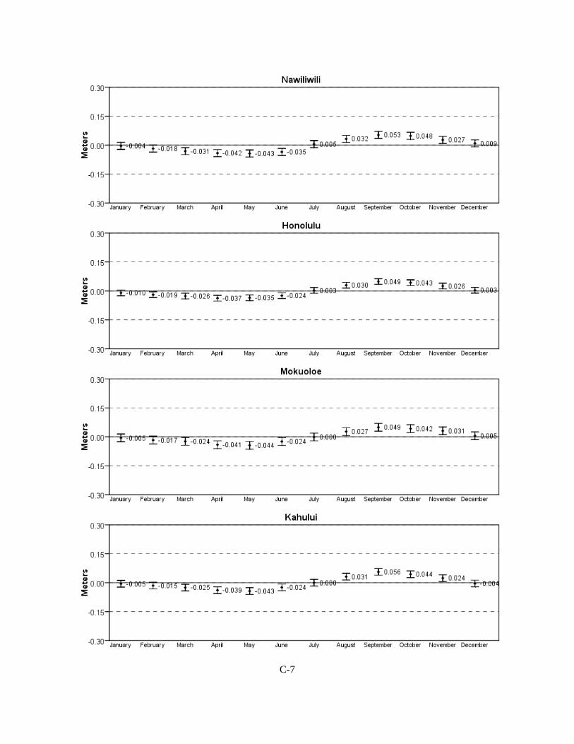
C-7

 

 

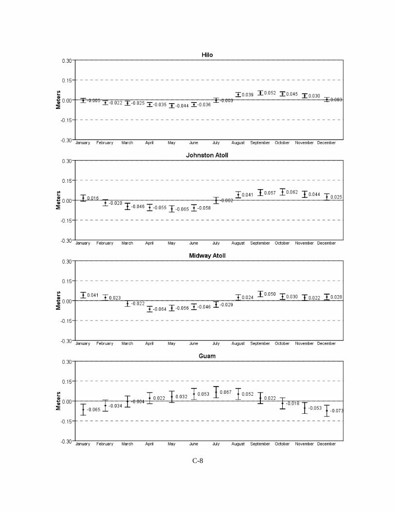
C-8

 

 

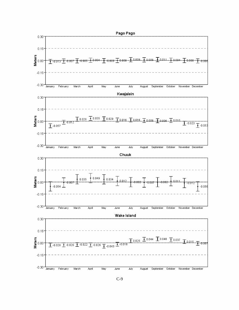
C-9

 

 

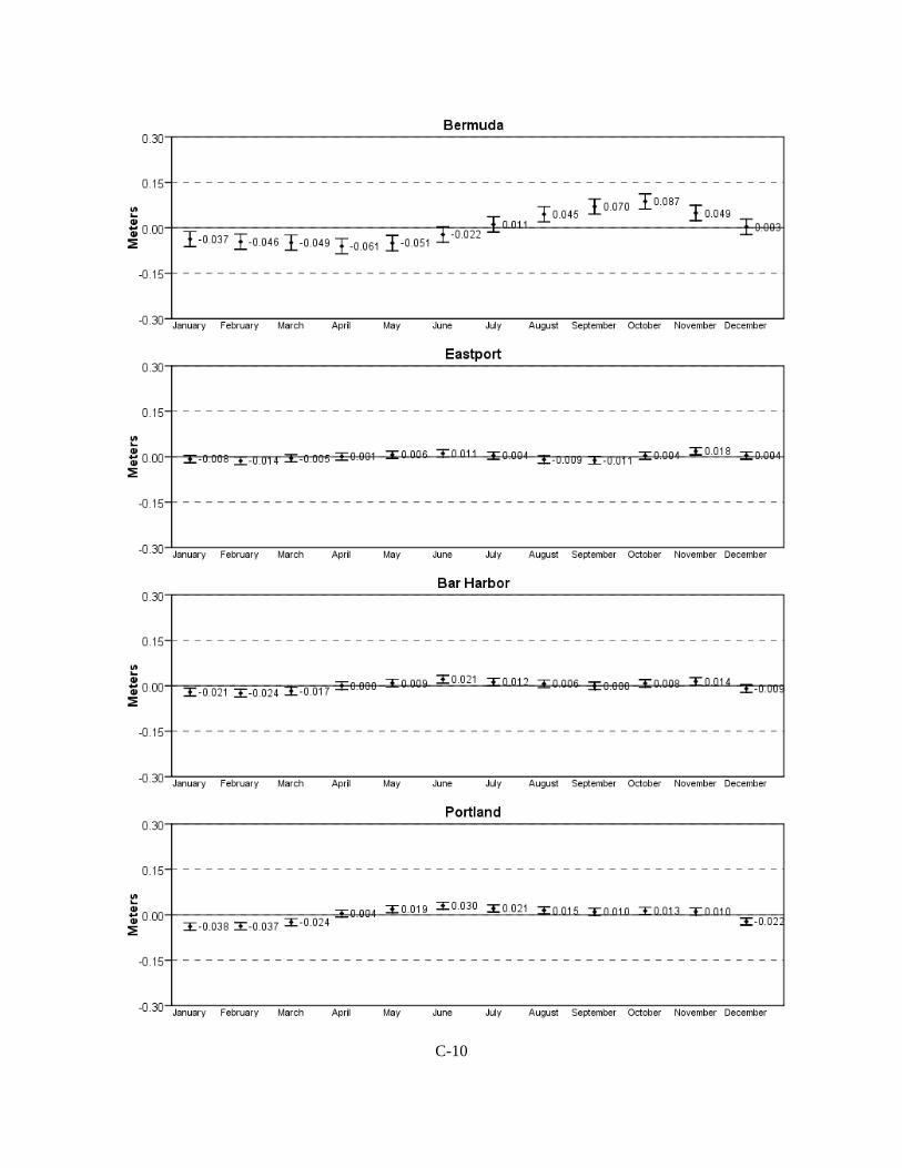
C-10

 

 

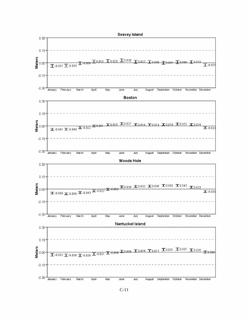
C-11

 

 

C-12

 

 

C-13

 

 

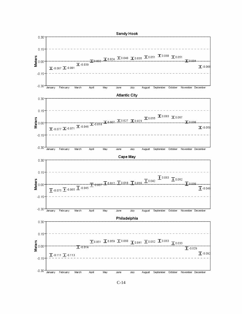
C-14

 

 

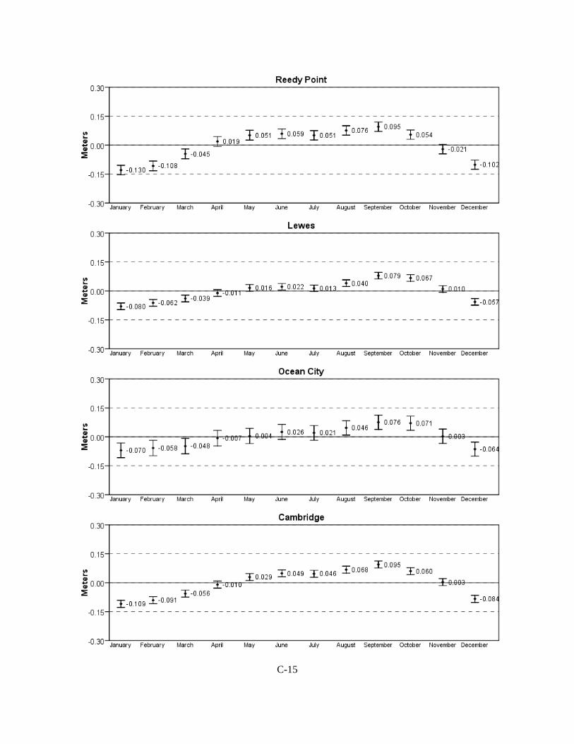
C-15

 

 

C-16

 

 

C-17

 

 

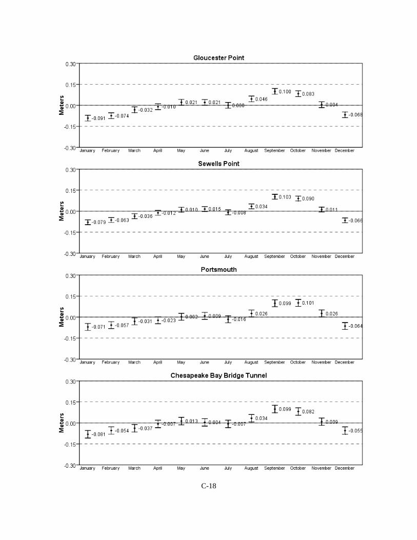
C-18

 

 

C-19

 

 

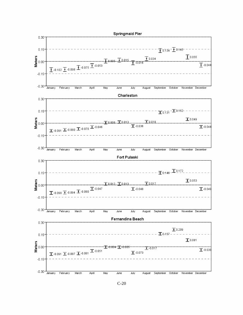
C-20

 

 

C-21

 

 

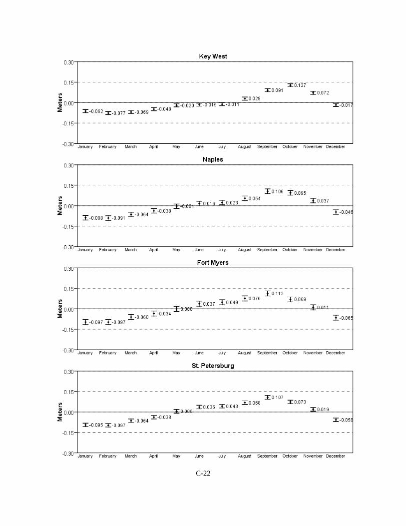
C-22

 

 

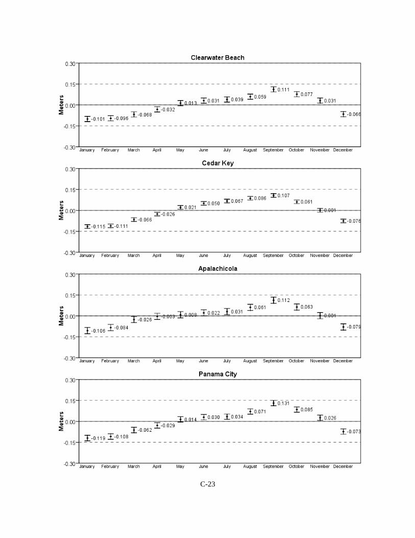
C-23

 

 

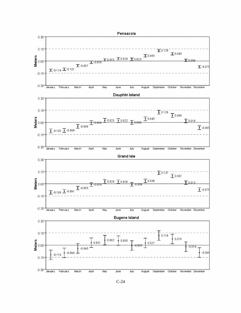
C-24

 

 

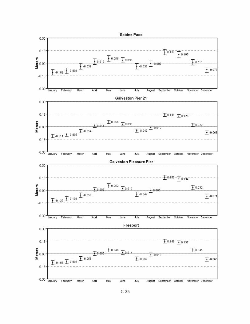
C-25

 

 

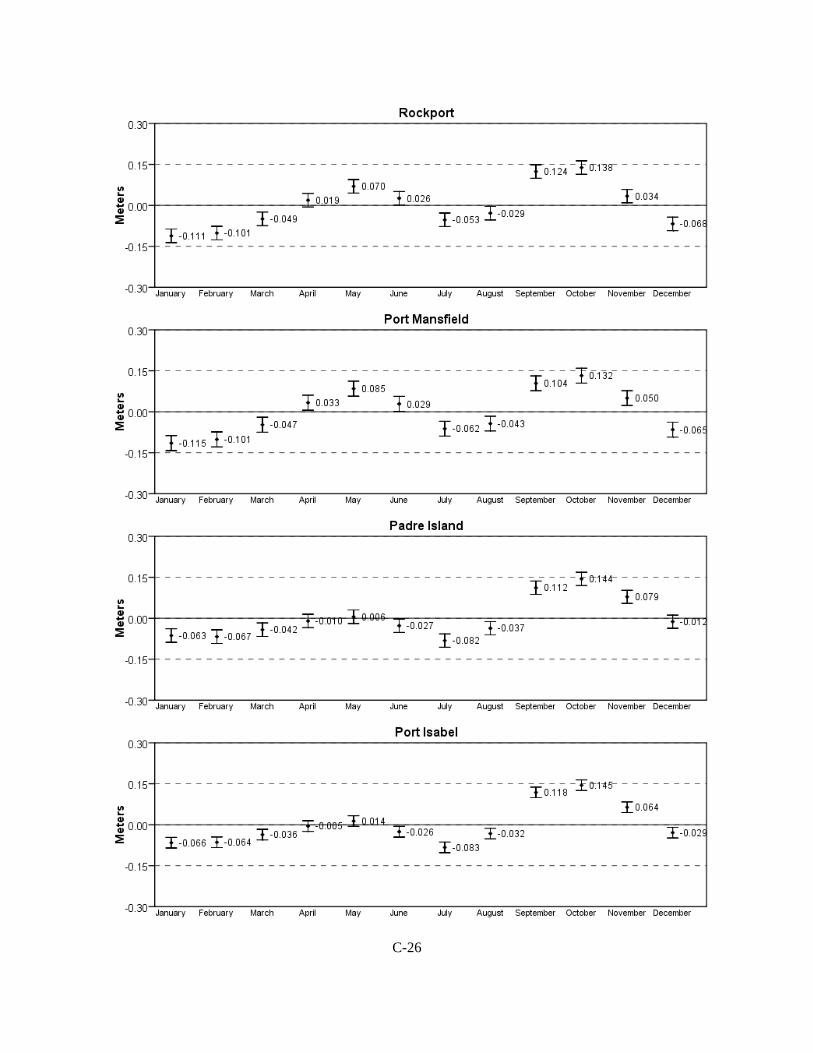
C-26

 

 

C-27

 

 

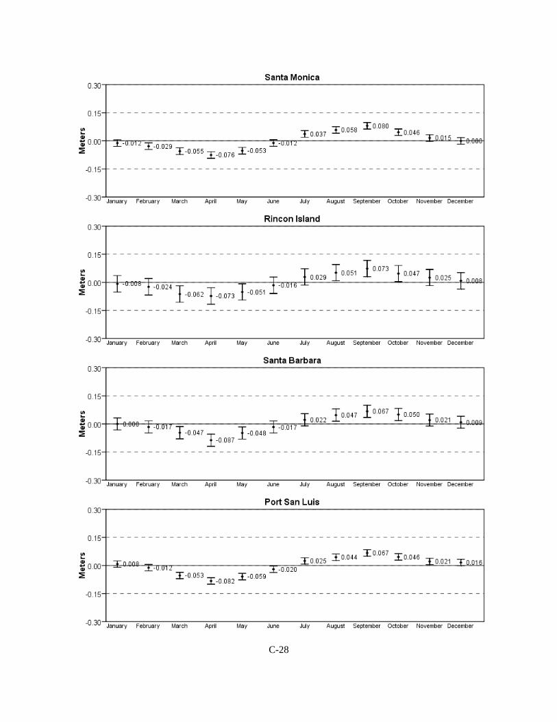
C-28

 

 

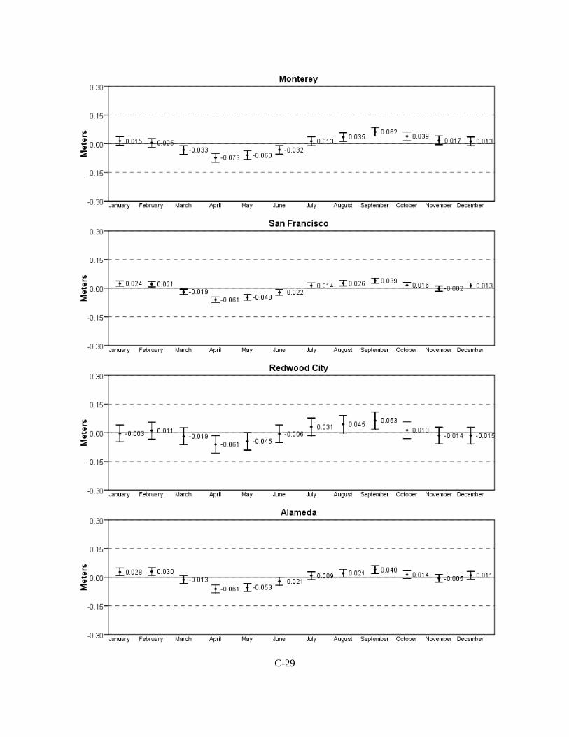
C-29

 

 

C-30

 

 

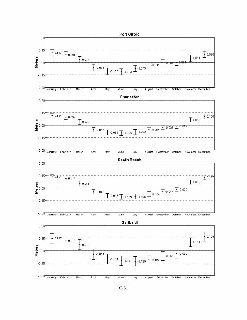
C-31

 

 

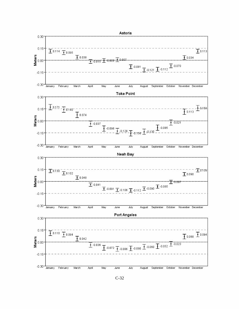
C-32

 

 

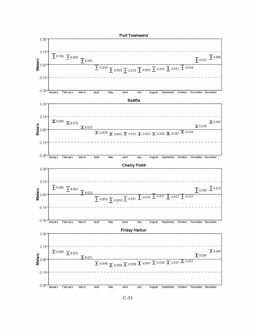
C-33

 

 

C-34

 

 

C-35

 

 

C-36

 

 

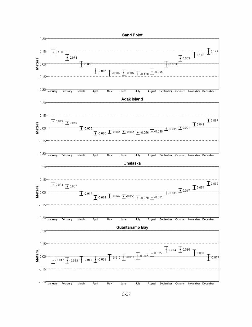
C-37

 

 

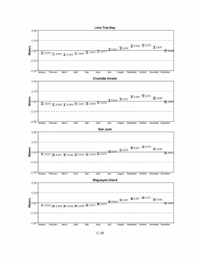
C-38

 

 

D-1

APPENDIX IV

Comparison of Sa and Ssa tidal constituents

derived from average seasonal cycles

with the accepted tidal constituents

used for CO-OPS tide predictions

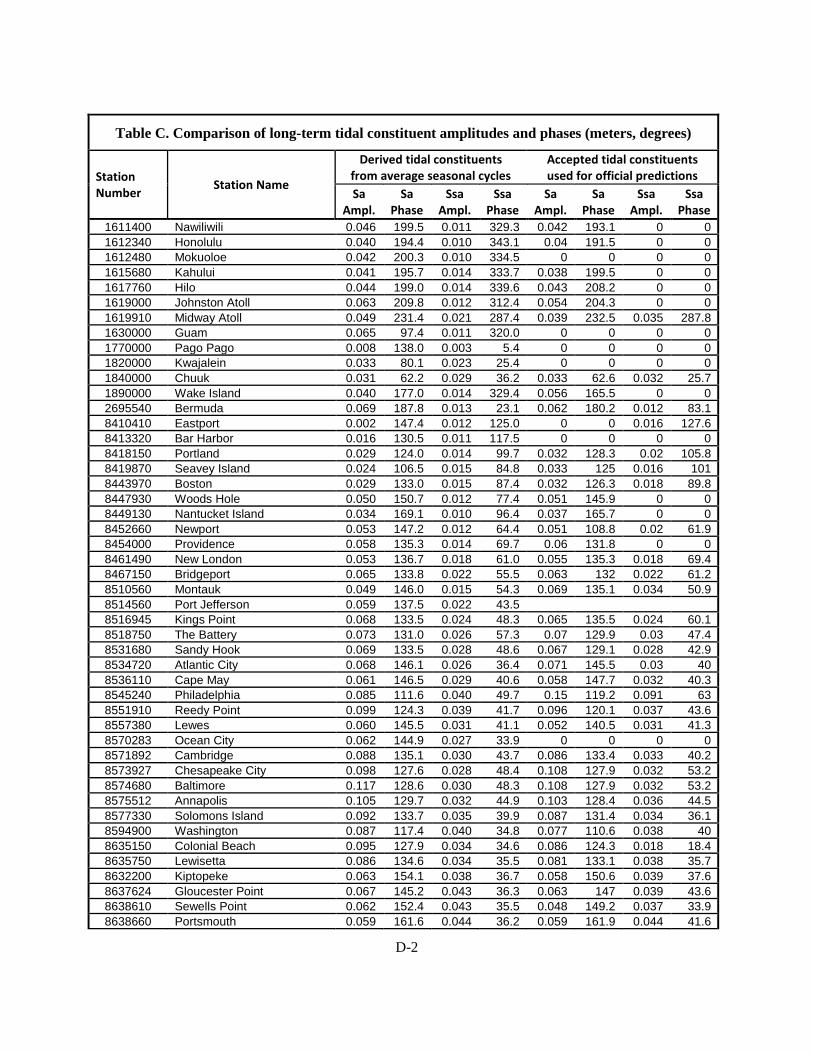
D-2

Table C. Comparison of long-term tidal constituent amplitudes and phases (meters, degrees)

Station Number

Station Name

Derived tidal constituents from average seasonal cycles

Accepted tidal constituents used for official predictions

Sa Ampl.

Sa Phase

Ssa Ampl.

Ssa Phase

Sa Ampl.

Sa Phase

Ssa Ampl.

Ssa Phase

1611400 Nawiliwili 0.046 199.5 0.011 329.3 0.042 193.1 0 0

1612340 Honolulu 0.040 194.4 0.010 343.1 0.04 191.5 0 0

1612480 Mokuoloe 0.042 200.3 0.010 334.5 0 0 0 0

1615680 Kahului 0.041 195.7 0.014 333.7 0.038 199.5 0 0

1617760 Hilo 0.044 199.0 0.014 339.6 0.043 208.2 0 0

1619000 Johnston Atoll 0.063 209.8 0.012 312.4 0.054 204.3 0 0

1619910 Midway Atoll 0.049 231.4 0.021 287.4 0.039 232.5 0.035 287.8

1630000 Guam 0.065 97.4 0.011 320.0 0 0 0 0

1770000 Pago Pago 0.008 138.0 0.003 5.4 0 0 0 0

1820000 Kwajalein 0.033 80.1 0.023 25.4 0 0 0 0

1840000 Chuuk 0.031 62.2 0.029 36.2 0.033 62.6 0.032 25.7

1890000 Wake Island 0.040 177.0 0.014 329.4 0.056 165.5 0 0

2695540 Bermuda 0.069 187.8 0.013 23.1 0.062 180.2 0.012 83.1

8410410 Eastport 0.002 147.4 0.012 125.0 0 0 0.016 127.6

8413320 Bar Harbor 0.016 130.5 0.011 117.5 0 0 0 0

8418150 Portland 0.029 124.0 0.014 99.7 0.032 128.3 0.02 105.8

8419870 Seavey Island 0.024 106.5 0.015 84.8 0.033 125 0.016 101

8443970 Boston 0.029 133.0 0.015 87.4 0.032 126.3 0.018 89.8

8447930 Woods Hole 0.050 150.7 0.012 77.4 0.051 145.9 0 0

8449130 Nantucket Island 0.034 169.1 0.010 96.4 0.037 165.7 0 0

8452660 Newport 0.053 147.2 0.012 64.4 0.051 108.8 0.02 61.9

8454000 Providence 0.058 135.3 0.014 69.7 0.06 131.8 0 0

8461490 New London 0.053 136.7 0.018 61.0 0.055 135.3 0.018 69.4

8467150 Bridgeport 0.065 133.8 0.022 55.5 0.063 132 0.022 61.2

8510560 Montauk 0.049 146.0 0.015 54.3 0.069 135.1 0.034 50.9

8514560 Port Jefferson 0.059 137.5 0.022 43.5

8516945 Kings Point 0.068 133.5 0.024 48.3 0.065 135.5 0.024 60.1

8518750 The Battery 0.073 131.0 0.026 57.3 0.07 129.9 0.03 47.4

8531680 Sandy Hook 0.069 133.5 0.028 48.6 0.067 129.1 0.028 42.9

8534720 Atlantic City 0.068 146.1 0.026 36.4 0.071 145.5 0.03 40

8536110 Cape May 0.061 146.5 0.029 40.6 0.058 147.7 0.032 40.3

8545240 Philadelphia 0.085 111.6 0.040 49.7 0.15 119.2 0.091 63

8551910 Reedy Point 0.099 124.3 0.039 41.7 0.096 120.1 0.037 43.6

8557380 Lewes 0.060 145.5 0.031 41.1 0.052 140.5 0.031 41.3

8570283 Ocean City 0.062 144.9 0.027 33.9 0 0 0 0

8571892 Cambridge 0.088 135.1 0.030 43.7 0.086 133.4 0.033 40.2

8573927 Chesapeake City 0.098 127.6 0.028 48.4 0.108 127.9 0.032 53.2

8574680 Baltimore 0.117 128.6 0.030 48.3 0.108 127.9 0.032 53.2

8575512 Annapolis 0.105 129.7 0.032 44.9 0.103 128.4 0.036 44.5

8577330 Solomons Island 0.092 133.7 0.035 39.9 0.087 131.4 0.034 36.1

8594900 Washington 0.087 117.4 0.040 34.8 0.077 110.6 0.038 40

8635150 Colonial Beach 0.095 127.9 0.034 34.6 0.086 124.3 0.018 18.4

8635750 Lewisetta 0.086 134.6 0.034 35.5 0.081 133.1 0.038 35.7

8632200 Kiptopeke 0.063 154.1 0.038 36.7 0.058 150.6 0.039 37.6

8637624 Gloucester Point 0.067 145.2 0.043 36.3 0.063 147 0.039 43.6

8638610 Sewells Point 0.062 152.4 0.043 35.5 0.048 149.2 0.037 33.9

8638660 Portsmouth 0.059 161.6 0.044 36.2 0.059 161.9 0.044 41.6

D-3

Table C. Comparison of long-term tidal constituent amplitudes and phases (meters, degrees)

Station Number

Station Name

Derived tidal constituents from average seasonal cycles

Accepted tidal constituents used for official predictions

Sa Ampl.

Sa Phase

Ssa Ampl.

Ssa Phase

Sa Ampl.

Sa Phase

Ssa Ampl.

Ssa Phase

8638863 Ches Bay Bridge Tunnel 0.058 152.7 0.041 34.5 0.055 152 0.042 34

8652587 Oregon Inlet Marina 0.062 154.2 0.026 45.0 0.046 158.9 0.026 10.5

8656483 Beaufort 0.071 165.8 0.041 46.4 0.066 166 0.036 57.1

8658120 Wilmington 0.044 151.1 0.038 25.7 0 0 0.051 24.9

8659084 Southport 0.070 167.6 0.042 57.2 0 0 0 0

8661070 Springmaid Pier 0.094 168.3 0.053 53.9 0.083 170.9 0.053 50.1

8665530 Charleston 0.084 172.3 0.057 51.9 0.078 176.3 0.053 50.5

8670870 Fort Pulaski 0.093 172.7 0.066 52.9 0.084 176 0.06 51.8

8720030 Fernandina Beach 0.098 186.2 0.079 55.0 0.086 119.6 0.07 54.7

8720218 Mayport 0.105 192.9 0.073 53.9 0.115 190.2 0.077 55.4

8721120 Daytona Beach Shores 0.097 200.2 0.065 62.3 0.104 197.5 0.077 52.4

8723170 Miami Beach 0.084 196.5 0.053 66.5 0.088 198.8 0.062 68.7

8723970 Vaca Key 0.079 190.2 0.038 59.0 0.083 196.1 0.033 70.5

8724580 Key West 0.080 182.6 0.039 58.4 0.08 187.8 0.041 56.5

8725110 Naples 0.083 159.4 0.032 47.8 0.075 167.9 0.03 66.7

8725520 Fort Myers 0.092 146.6 0.024 32.1 0.082 150.7 0 0

8726520 St. Petersburg 0.090 149.0 0.025 44.6 0.092 150.8 0.033 41

8726724 Clearwater Beach 0.089 149.3 0.032 49.3 0.091 151.9 0.037 48.2

8727520 Cedar Key 0.102 138.6 0.024 41.9 0.096 136.4 0 0

8728690 Apalachicola 0.078 139.9 0.041 24.9 0.075 145.1 0.036 28.7

8729108 Panama City 0.098 148.1 0.040 41.4 0.095 150.6 0.034 48.9

8729840 Pensacola 0.091 146.6 0.043 37.8 0.087 148.3 0.048 43.2

8735180 Dauphin Island 0.079 147.8 0.050 44.2 0.08 156.3 0.05 51.3

8761724 Grand Isle 0.080 148.9 0.053 42.9 0.087 149.7 0.06 49.7

8764311 Eugene Island 0.079 126.1 0.057 47.3 0 0 0 0

8770570 Sabine Pass 0.065 141.5 0.071 51.5 0.065 135.7 0.077 52

8771450 Galveston Pier 21 0.069 150.7 0.076 54.3 0.066 155.7 0.086 55.6

8771510 Galveston Pleasure Pier 0.077 153.9 0.081 52.1 0.077 157.4 0.09 55.2

8772440 Freeport 0.070 161.9 0.081 54.1 0.057 173.5 0.074 64.3

8774770 Rockport 0.063 151.0 0.085 59.7 0.061 161 0.09 69.9

8778490 Port Mansfield 0.055 147.5 0.093 64.9

8779750 Padre Island 0.063 199.1 0.072 57.3 0.081 206.6 0.085 56.2

8779770 Port Isabel 0.058 193.9 0.074 52.5 0.055 196.1 0.069 58.8

9410170 San Diego 0.067 183.1 0.015 269.7 0.069 179.3 0 0

9410230 La Jolla 0.069 182.6 0.015 271.8 0.07 184.3 0.017 263.2

9410580 Newport Beach 0.063 184.1 0.017 278.5 0.063 183.4 0.014 280.2

9410660 Los Angeles 0.064 184.4 0.016 268.9 0.066 184.4 0 0

9410840 Santa Monica 0.063 180.8 0.019 279.3 0.065 183.2 0 0

9411270 Rincon Island 0.062 186.2 0.015 271.1

9411340 Santa Barbara 0.059 191.0 0.017 272.5 0.079 156.8 0 0

9412110 Port San Luis 0.059 194.9 0.020 265.7 0.056 191.9 0.032 279.1

9413450 Monterey 0.050 204.8 0.023 282.2 0.048 206 0.027 283.9

9414290 San Francisco 0.032 212.7 0.027 270.1 0.038 221.4 0.039 286.9

9414523 Redwood City 0.030 220.0 0.029 274.0 0.038 221.4 0.039 286.9

9414750 Alameda 0.022 198.6 0.021 261.6 0.032 227.8 0.037 288.3

9415144 Port Chicago 0.005 146.2 0.048 278.6 0 0 0.06 285.7

9415020 Point Reyes 0.055 220.7 0.034 277.0 0.061 217.7 0.031 285.3

9418767 North Spit 0.069 257.5 0.035 269.8 0.065 255 0.038 264.1

D-4

Table C. Comparison of long-term tidal constituent amplitudes and phases (meters, degrees)

Station Number

Station Name

Derived tidal constituents from average seasonal cycles

Accepted tidal constituents used for official predictions

Sa Ampl.

Sa Phase

Ssa Ampl.

Ssa Phase

Sa Ampl.

Sa Phase

Ssa Ampl.

Ssa Phase

9419750 Crescent City 0.075 260.7 0.034 257.2 0.071 261.4 0.041 262.1

9431647 Port Orford 0.102 273.5 0.033 271.9 0.093 268 0 0

9432780 Charleston 0.104 280.5 0.025 250.8 0.103 283.3 0 0

9435380 South Beach 0.124 285.2 0.025 247.0 0.123 281.6 0.019 258.7

9437540 Garibaldi 0.150 287.4 0.022 216.5 0 0 0 0

9439040 Astoria 0.101 314.2 0.048 178.3 0.111 307.2 0.052 184.1

9440910 Toke Point 0.167 290.2 0.018 201.6 0.158 289.8 0 0

9443090 Neah Bay 0.130 285.0 0.018 210.6 0.126 289.9 0 0

9444090 Port Angeles 0.100 287.4 0.020 236.5 0.101 287.6 0 0

9444900 Port Townsend 0.087 290.7 0.024 236.0 0.082 292 0 0

9447130 Seattle 0.076 289.8 0.027 222.3 0.077 292.9 0.033 231.1

9449424 Cherry Point 0.065 277.1 0.029 238.5 0.05 280.1 0.023 236.5

9449880 Friday Harbor 0.076 281.5 0.028 228.1 0.085 280.4 0.039 221

9450460 Ketchikan 0.108 266.4 0.026 146.6 0.115 273.7 0.031 161.1

9451600 Sitka 0.119 267.6 0.018 125.9 0.121 274.8 0 0

9452210 Juneau 0.082 235.8 0.021 145.1 0.08 255.6 0 0

9452400 Skagway 0.086 194.2 0.015 168.7 0.059 190 0 0

9453220 Yakutat 0.122 255.6 0.016 100.9 0.122 265.1 0.033 59.8

9454050 Cordova 0.123 248.1 0.010 56.1 0.131 254.2 0 0

9454240 Valdez 0.108 239.6 0.002 128.5 0.112 243.1 0 0

9455090 Seward 0.125 245.5 0.012 80.7 0.118 253.3 0 0

9455500 Seldovia 0.119 251.6 0.014 67.0 0.116 251.4 0.017 70.8

9455760 Nikiski 0.105 240.7 0.009 221.1 0.12 243.7 0 0

9455920 Anchorage 0.088 213.6 0.017 245.0 0.054 230.2 0.072 45.6

9457292 Kodiak Island 0.083 249.1 0.004 143.4 0.078 262.1 0.015 151.7

9459450 Sand Point 0.137 266.7 0.014 182.2 0.123 272.3 0 0

9462620 Unalaska 0.080 271.4 0.020 193.4 0.094 277.7 0.039 216.2

9461380 Adak Island 0.068 272.1 0.022 214.5 0.076 269.4 0.021 206.2

9731158 Guantanamo Bay 0.058 176.9 0.023 40.2

9751401 Lime Tree Bay 0.062 181.0 0.013 57.4 0.059 184.9 0.015 60

9751639 Charlotte Amalie 0.059 183.4 0.017 43.0 0.061 181.8 0.019 47.2

9755371 San Juan 0.055 185.9 0.018 32.3 0.055 186.9 0.021 37.1

9759110 Magueyes Island 0.061 182.3 0.013 37.8 0.062 184.2 0.016 42.6

E-1

Appendix V

Linear trends for 50-year periods

of mean sea level data

Note Derived 50-year linear trends and 95% confidence intervals of the trends are shown for stations with over 80 years of data. Solid horizontal line shows linear trend derived from station’s entire data set.

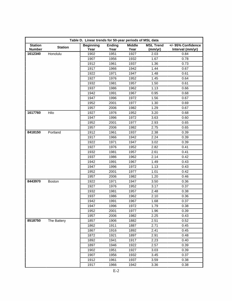
E-2

Table D. Linear trends for 50-year periods of MSL data

Station Number

Station Beginning

Year Ending

Year Middle Year

MSL Trend (mm/yr)

+/- 95% Confidence Interval (mm/yr)

1612340 Honolulu 1902 1951 1927 2.03 0.84

1907 1956 1932 1.67 0.78

1912 1961 1937 1.36 0.73

1917 1966 1942 1.44 0.67

1922 1971 1947 1.48 0.61

1927 1976 1952 1.45 0.64

1932 1981 1957 1.50 0.61

1937 1986 1962 1.13 0.66

1942 1991 1967 0.95 0.68

1947 1996 1972 1.56 0.67

1952 2001 1977 1.30 0.69

1957 2006 1982 1.29 0.67

1617760 Hilo 1927 1976 1952 3.20 0.68

1947 1996 1972 3.63 0.60

1952 2001 1977 2.93 0.65

1957 2006 1982 2.75 0.65

8418150 Portland 1912 1961 1937 2.38 0.39

1917 1966 1942 2.24 0.39

1922 1971 1947 3.02 0.39

1927 1976 1952 2.82 0.41

1932 1981 1957 2.61 0.41

1937 1986 1962 2.14 0.42

1942 1991 1967 1.49 0.43

1947 1996 1972 1.13 0.43

1952 2001 1977 1.01 0.42

1957 2006 1982 1.20 0.46

8443970 Boston 1922 1971 1947 3.50 0.36

1927 1976 1952 3.17 0.37

1932 1981 1957 2.48 0.38

1937 1986 1962 2.10 0.36

1942 1991 1967 1.68 0.37

1947 1996 1972 1.79 0.38

1952 2001 1977 1.96 0.39

1957 2006 1982 2.25 0.43

8518750 The Battery 1857 1906 1882 2.51 0.52

1862 1911 1887 2.71 0.45

1867 1916 1892 2.41 0.45

1872 1921 1897 2.91 0.48

1892 1941 1917 2.23 0.40

1897 1946 1922 2.57 0.39

1902 1951 1927 3.03 0.39

1907 1956 1932 3.45 0.37

1912 1961 1937 3.59 0.38

1917 1966 1942 3.36 0.38

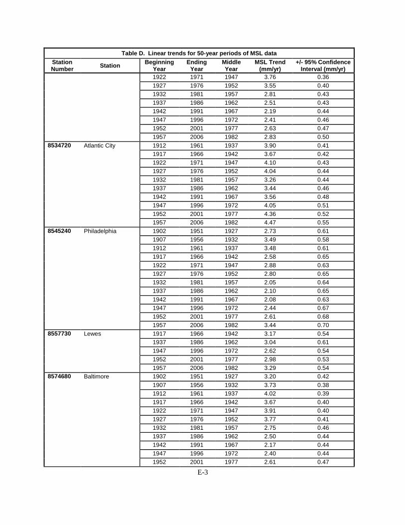
E-3

Table D. Linear trends for 50-year periods of MSL data

Station Number

Station Beginning

Year Ending

Year Middle Year

MSL Trend (mm/yr)

+/- 95% Confidence Interval (mm/yr)

1922 1971 1947 3.76 0.36

1927 1976 1952 3.55 0.40

1932 1981 1957 2.81 0.43

1937 1986 1962 2.51 0.43

1942 1991 1967 2.19 0.44

1947 1996 1972 2.41 0.46

1952 2001 1977 2.63 0.47

1957 2006 1982 2.83 0.50

8534720 Atlantic City 1912 1961 1937 3.90 0.41

1917 1966 1942 3.67 0.42

1922 1971 1947 4.10 0.43

1927 1976 1952 4.04 0.44

1932 1981 1957 3.26 0.44

1937 1986 1962 3.44 0.46

1942 1991 1967 3.56 0.48

1947 1996 1972 4.05 0.51

1952 2001 1977 4.36 0.52

1957 2006 1982 4.47 0.55

8545240 Philadelphia 1902 1951 1927 2.73 0.61

1907 1956 1932 3.49 0.58

1912 1961 1937 3.48 0.61

1917 1966 1942 2.58 0.65

1922 1971 1947 2.88 0.63

1927 1976 1952 2.80 0.65

1932 1981 1957 2.05 0.64

1937 1986 1962 2.10 0.65

1942 1991 1967 2.08 0.63

1947 1996 1972 2.44 0.67

1952 2001 1977 2.61 0.68

1957 2006 1982 3.44 0.70

8557730 Lewes 1917 1966 1942 3.17 0.54

1937 1986 1962 3.04 0.61

1947 1996 1972 2.62 0.54

1952 2001 1977 2.98 0.53

1957 2006 1982 3.29 0.54

8574680 Baltimore 1902 1951 1927 3.20 0.42

1907 1956 1932 3.73 0.38

1912 1961 1937 4.02 0.39

1917 1966 1942 3.67 0.40

1922 1971 1947 3.91 0.40

1927 1976 1952 3.77 0.41

1932 1981 1957 2.75 0.46

1937 1986 1962 2.50 0.44

1942 1991 1967 2.17 0.44

1947 1996 1972 2.40 0.44

1952 2001 1977 2.61 0.47

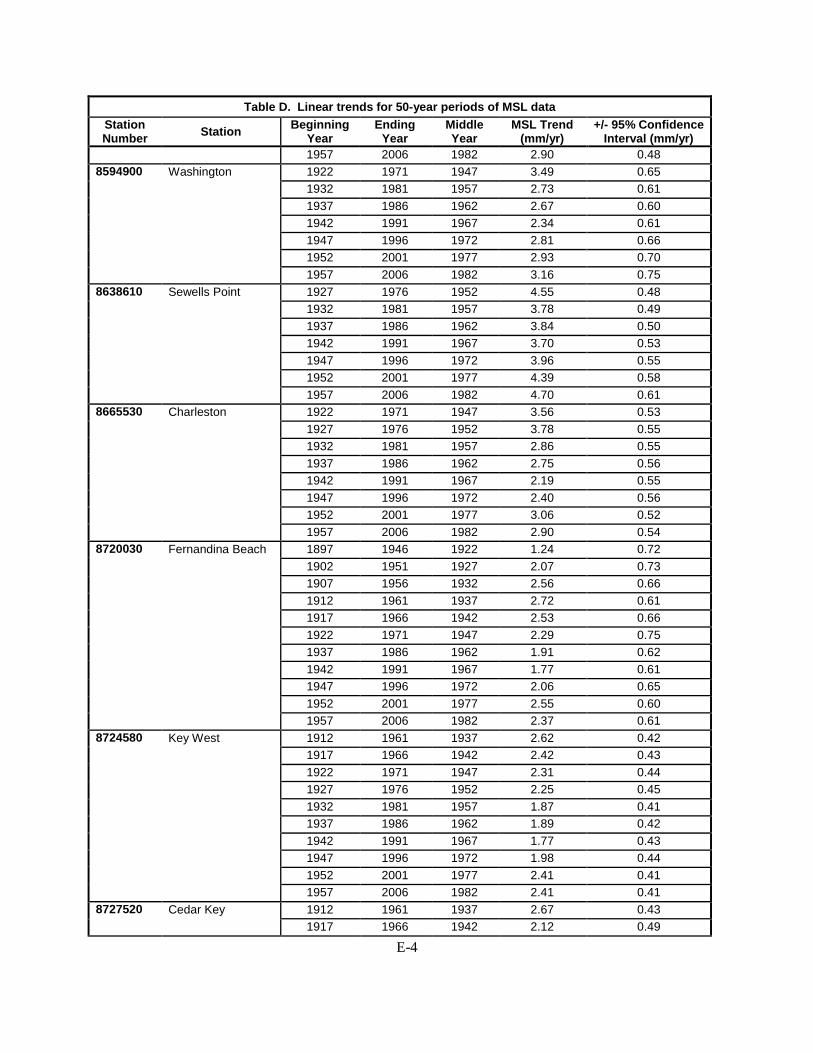
E-4

Table D. Linear trends for 50-year periods of MSL data

Station Number

Station Beginning

Year Ending

Year Middle Year

MSL Trend (mm/yr)

+/- 95% Confidence Interval (mm/yr)

1957 2006 1982 2.90 0.48

8594900 Washington 1922 1971 1947 3.49 0.65

1932 1981 1957 2.73 0.61

1937 1986 1962 2.67 0.60

1942 1991 1967 2.34 0.61

1947 1996 1972 2.81 0.66

1952 2001 1977 2.93 0.70

1957 2006 1982 3.16 0.75

8638610 Sewells Point 1927 1976 1952 4.55 0.48

1932 1981 1957 3.78 0.49

1937 1986 1962 3.84 0.50

1942 1991 1967 3.70 0.53

1947 1996 1972 3.96 0.55

1952 2001 1977 4.39 0.58

1957 2006 1982 4.70 0.61

8665530 Charleston 1922 1971 1947 3.56 0.53

1927 1976 1952 3.78 0.55

1932 1981 1957 2.86 0.55

1937 1986 1962 2.75 0.56

1942 1991 1967 2.19 0.55

1947 1996 1972 2.40 0.56

1952 2001 1977 3.06 0.52

1957 2006 1982 2.90 0.54

8720030 Fernandina Beach 1897 1946 1922 1.24 0.72

1902 1951 1927 2.07 0.73

1907 1956 1932 2.56 0.66

1912 1961 1937 2.72 0.61

1917 1966 1942 2.53 0.66

1922 1971 1947 2.29 0.75

1937 1986 1962 1.91 0.62

1942 1991 1967 1.77 0.61

1947 1996 1972 2.06 0.65

1952 2001 1977 2.55 0.60

1957 2006 1982 2.37 0.61

8724580 Key West 1912 1961 1937 2.62 0.42

1917 1966 1942 2.42 0.43

1922 1971 1947 2.31 0.44

1927 1976 1952 2.25 0.45

1932 1981 1957 1.87 0.41

1937 1986 1962 1.89 0.42

1942 1991 1967 1.77 0.43

1947 1996 1972 1.98 0.44

1952 2001 1977 2.41 0.41

1957 2006 1982 2.41 0.41

8727520 Cedar Key 1912 1961 1937 2.67 0.43

1917 1966 1942 2.12 0.49

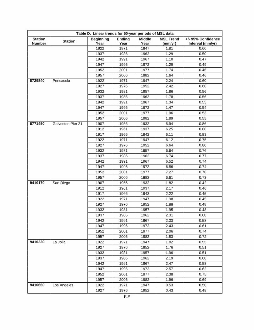
E-5

Table D. Linear trends for 50-year periods of MSL data

Station Number

Station Beginning

Year Ending

Year Middle Year

MSL Trend (mm/yr)

+/- 95% Confidence Interval (mm/yr)

1922 1971 1947 1.81 0.60

1937 1986 1962 1.29 0.50

1942 1991 1967 1.10 0.47

1947 1996 1972 1.29 0.49

1952 2001 1977 1.74 0.46

1957 2006 1982 1.64 0.46

8729840 Pensacola 1922 1971 1947 2.24 0.60

1927 1976 1952 2.42 0.60

1932 1981 1957 1.86 0.56

1937 1986 1962 1.78 0.56

1942 1991 1967 1.34 0.55

1947 1996 1972 1.47 0.54

1952 2001 1977 1.96 0.53

1957 2006 1982 1.89 0.55

8771450 Galveston Pier 21 1907 1956 1932 5.94 0.86

1912 1961 1937 6.25 0.80

1917 1966 1942 6.11 0.83

1922 1971 1947 6.12 0.75

1927 1976 1952 6.64 0.80

1932 1981 1957 6.64 0.76

1937 1986 1962 6.74 0.77

1942 1991 1967 6.52 0.74

1947 1996 1972 6.86 0.74

1952 2001 1977 7.27 0.70

1957 2006 1982 6.61 0.73

9410170 San Diego 1907 1956 1932 1.82 0.42

1912 1961 1937 2.17 0.46

1917 1966 1942 2.22 0.45

1922 1971 1947 1.98 0.45

1927 1976 1952 1.88 0.48

1932 1981 1957 1.95 0.48

1937 1986 1962 2.31 0.60

1942 1991 1967 2.33 0.58

1947 1996 1972 2.43 0.61

1952 2001 1977 2.06 0.74

1957 2006 1982 1.83 0.72

9410230 La Jolla 1922 1971 1947 1.82 0.55

1927 1976 1952 1.76 0.51

1932 1981 1957 1.96 0.51

1937 1986 1962 2.19 0.60

1942 1991 1967 2.47 0.58

1947 1996 1972 2.57 0.62

1952 2001 1977 2.38 0.75

1957 2006 1982 1.96 0.69

9410660 Los Angeles 1922 1971 1947 0.53 0.50

1927 1976 1952 0.43 0.48

E-6

Table D. Linear trends for 50-year periods of MSL data

Station Number

Station Beginning

Year Ending

Year Middle Year

MSL Trend (mm/yr)

+/- 95% Confidence Interval (mm/yr)

1932 1981 1957 0.48 0.48

1937 1986 1962 0.54 0.54

1942 1991 1967 0.57 0.52

1947 1996 1972 1.07 0.56

1952 2001 1977 0.97 0.66

1957 2006 1982 0.94 0.64

9414290 San Francisco 1852 1901 1877 1.14 0.94

1857 1906 1882 1.24 0.82

1862 1911 1887 0.26 0.77

1867 1916 1892 -0.24 0.68

1872 1921 1897 -0.40 0.66

1877 1926 1902 -0.67 0.63

1882 1931 1907 -0.17 0.59

1887 1936 1912 0.47 0.51

1892 1941 1917 1.46 0.59

1897 1946 1922 1.72 0.55

1902 1951 1927 1.60 0.53

1907 1956 1932 1.74 0.51

1912 1961 1937 2.01 0.54

1917 1966 1942 2.34 0.50

1922 1971 1947 2.43 0.52

1927 1976 1952 2.12 0.54

1932 1981 1957 1.84 0.58

1937 1986 1962 2.31 0.74

1942 1991 1967 2.18 0.68

1947 1996 1972 2.37 0.71

1952 2001 1977 2.01 0.78

1957 2006 1982 1.80 0.77

9439040 Astoria 1922 1971 1947 -0.10 0.81

1927 1976 1952 -0.16 0.77

1932 1981 1957 -0.76 0.79

1937 1986 1962 -0.34 0.87

1942 1991 1967 -0.89 0.86

1947 1996 1972 -0.96 0.84

1952 2001 1977 -0.30 0.87

1957 2006 1982 -0.19 0.84

9447130 Seattle 1897 1946 1922 1.06 0.50

1902 1951 1927 1.25 0.46

1907 1956 1932 1.65 0.46

1912 1961 1937 2.31 0.47

1917 1966 1942 2.57 0.47

1922 1971 1947 2.82 0.46

1927 1976 1952 2.57 0.47

1932 1981 1957 2.39 0.48

1937 1986 1962 2.60 0.56

1942 1991 1967 2.32 0.54

E-7

Table D. Linear trends for 50-year periods of MSL data

Station Number

Station Beginning

Year Ending

Year Middle Year

MSL Trend (mm/yr)

+/- 95% Confidence Interval (mm/yr)

1947 1996 1972 2.26 0.56

1952 2001 1977 2.09 0.62

1957 2006 1982 1.95 0.60

9450460 Ketchikan 1917 1966 1942 -0.29 0.62

1922 1971 1947 0.08 0.62

1927 1976 1952 -0.33 0.62

1932 1981 1957 -0.40 0.59

1937 1986 1962 -0.10 0.64

1942 1991 1967 0.06 0.61

1947 1996 1972 -0.02 0.64

1952 2001 1977 -0.27 0.68

1957 2006 1982 -0.38 0.69

9451600 Sitka 1922 1971 1947 -2.15 0.75

1937 1986 1962 -2.16 0.56

1942 1991 1967 -2.00 0.53

1947 1996 1972 -2.02 0.55

1952 2001 1977 -2.09 0.59

1957 2006 1982 -1.96 0.60

E-8

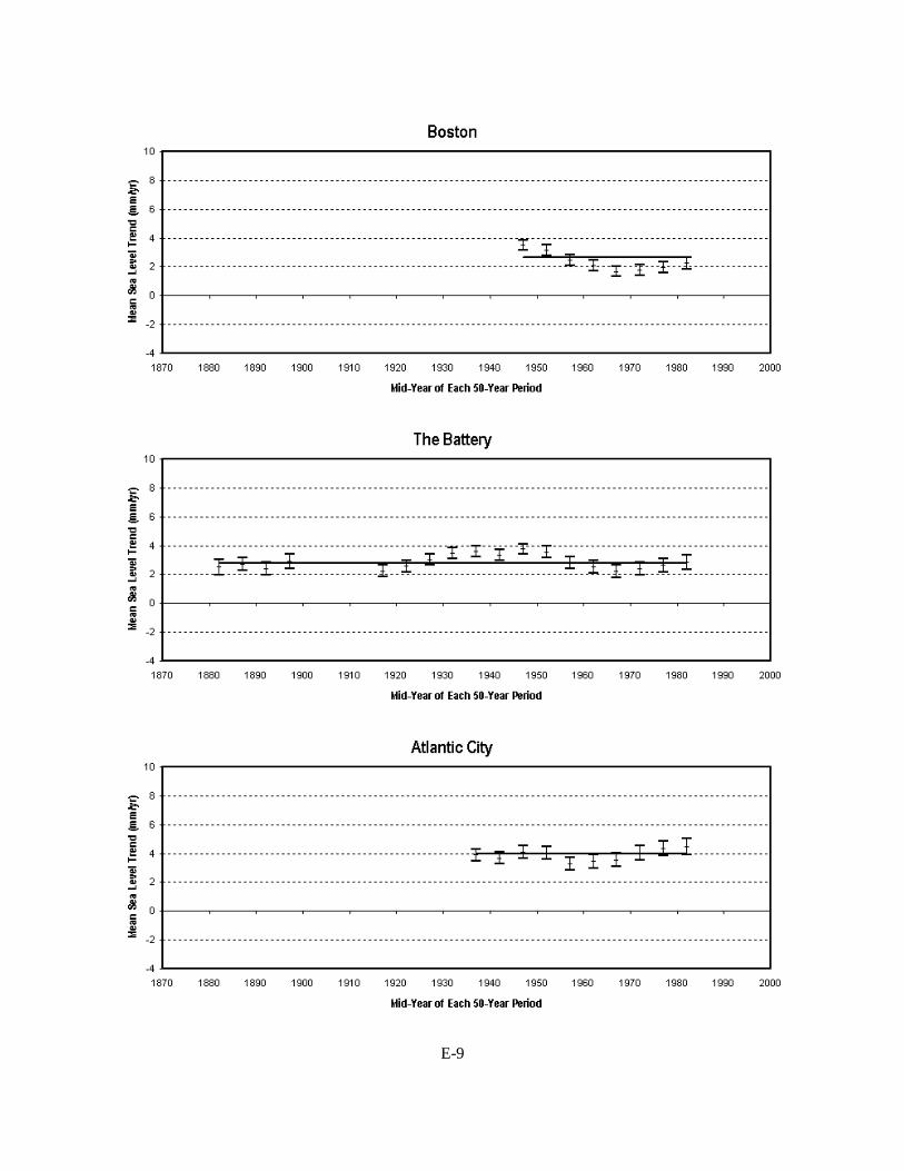
E-9

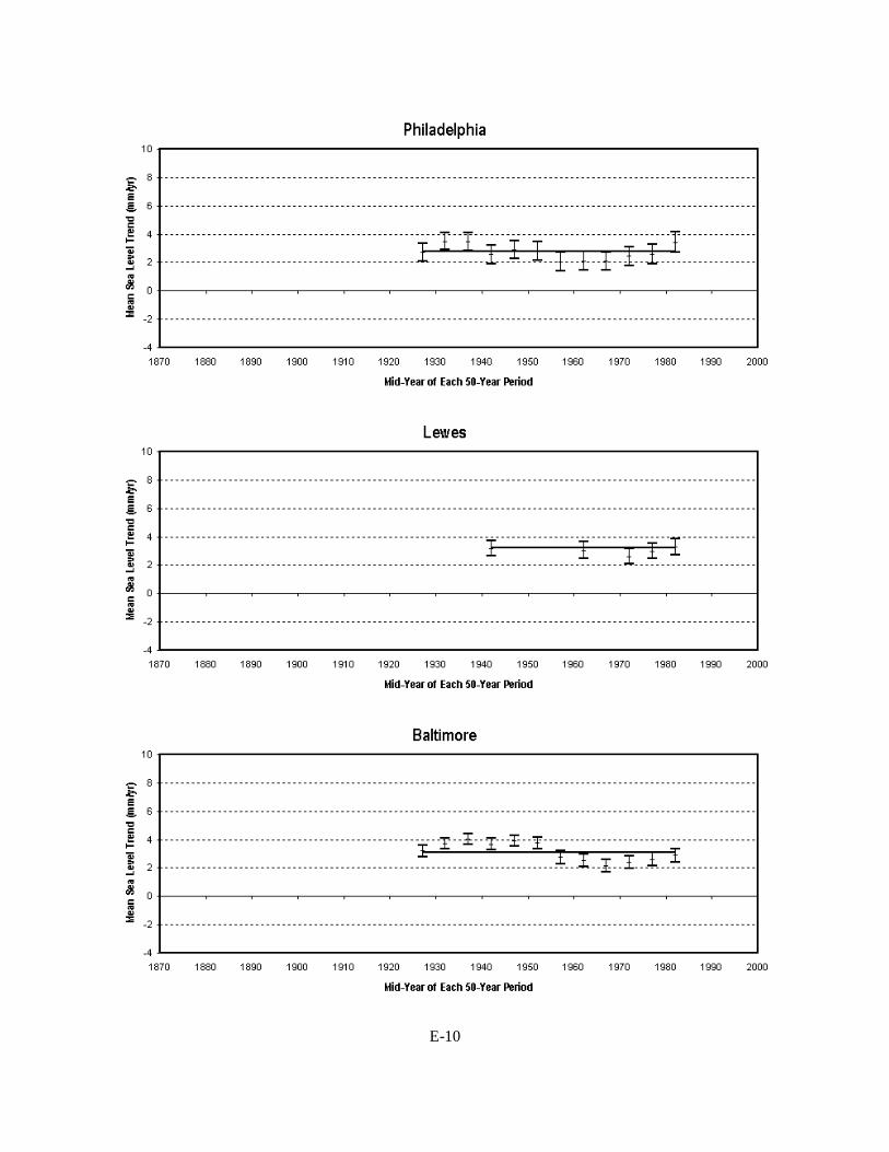
E-10

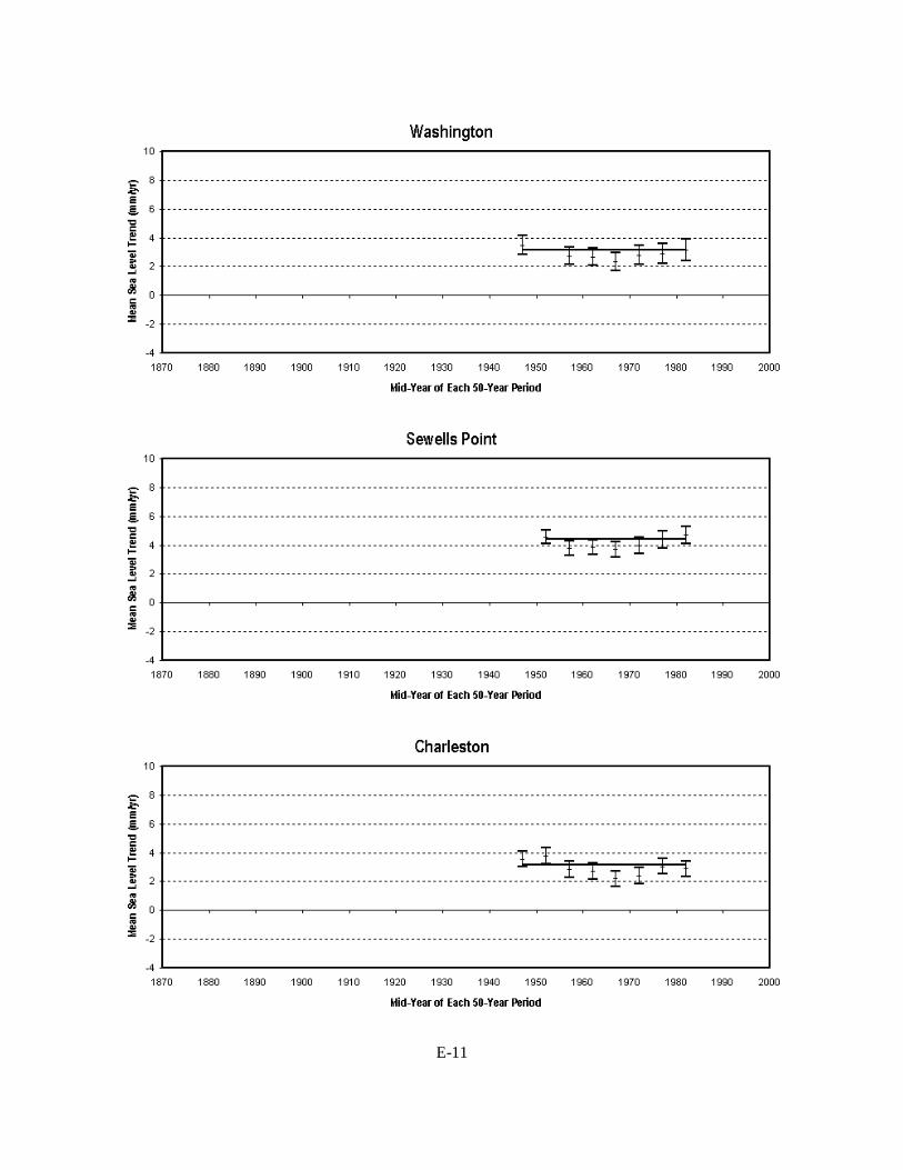
E-11

E-12

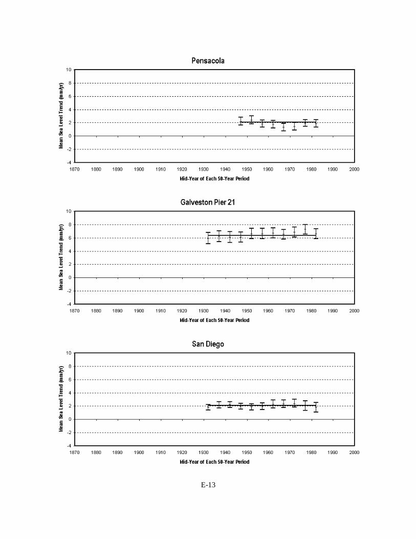
E-13

E-14

E-15

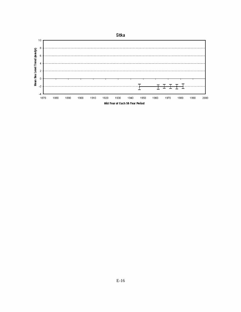
E-16

79

http://www.tidesandcurrents.noaa.gov/