Embed Size (px)
Citation preview

Sea Around UsResearch Protocol:
Catch reconstructions
June 30 2019


SEA AROUND US RESEARCH PROTOCOL: CATCH RECONSTRUCTIONS
Brittany Derrick,
Dirk Zeller,
Daniel Pauly
and
Maria. L.D. Palomares,
A report prepared by the Sea Around Us for the Minderoo Foundation
June 30, 2019
SEA AROUND US RESEARCH PROTOCOL: CATCH RECONSTRUCTIONS
B. Derrick, D. Zeller and D. Pauly and M.L.D. Palomares1
CITE AS: Derrick B, Zeller D, Pauly D and Palomares MLD (2019) Sea Around Us Research Protocol: Catch Reconstructions. A report prepared by the Sea Around Us for the Minderoo Foundation. The University of British Columbia, Vancouver, 74 p. Corresponding author: [email protected].
1 Sea Around Us, Institute for the Oceans and Fisheries, University of British Columbia, 2202 Main Mall, Vancouver BC V6T1Z4 Canada
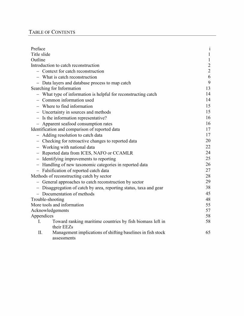
TABLE OF CONTENTS
Preface i Title slide 1 Outline 1 Introduction to catch reconstruction 2
− Context for catch reconstruction 2 − What is catch reconstruction 6 − Data layers and database process to map catch 9
Searching for Information 13 − What type of information is helpful for reconstructing catch 14 − Common information used 14 − Where to find information 15 − Uncertainty in sources and methods 15 − Is the information representative? 16 − Apparent seafood consumption rates 16
Identification and comparison of reported data 17 − Adding resolution to catch data 17 − Checking for retroactive changes to reported data 20 − Working with national data 22 − Reported data from ICES, NAFO or CCAMLR 24 − Identifying improvements to reporting 25 − Handling of new taxonomic categories in reported data 26 − Falsification of reported catch data 27
Methods of reconstructing catch by sector 28 − General approaches to catch reconstruction by sector 29 − Disaggregation of catch by area, reporting status, taxa and gear 38 − Documentation of methods 45
Trouble-shooting 48 More tools and information 55 Acknowledgements 57 Appendices 58
I. Toward ranking maritime countries by fish biomass left in their EEZs
58
II. Management implications of shifting baselines in fish stock assessments
65

i
PREFACE This report is a first product of a collaboration between the Minderoo Foundation and the Sea Around Us in view of the creation of a Global Fisheries Index (GFI). This report consists, in the main, the reproduction of a PowerPoint presentation (PPT) detailing how the Sea Around Us is currently (in 2019) updating the catch reconstruction that it assembled for all maritime countries of the world and their overseas territories for the year 1950 to 2010.
These reconstructions, in the last years, were summarily updated to 2014. However, for the purposes of the GFI, a thorough revision of all our procedures and specific catch reconstruction is warranted, and is being performed in the wake of an update to 2016. The PPT presented in this report documents how this updating and the concomitant review of our catch reconstructions will be proceeding.
Two appendices complete the report. The first is a paper presented at the Global Fishing Index Internal Project Review Meeting held at the Forrest Hall, UWA (Perth, Australia) on 13-15 May 2019. This meeting brought together the Minderoo Foundation, Sea Around Us and other groups. This paper presented the rationale for the contribution of the Sea Around Us to the GFI, and is included because the contribution was largely agreed upon, and thus, can serve as a guide to the further work by the Sea Around Us. The second appendix is based on a small study by a member of the Sea Around Us, Ms Rebecca Schijns, who demonstrated that the key method to be used by the Sea Around Us for the assessments that will form the basis of the GFI, the CMSY method, is extremely sensitive to the integrity of the catch time series used. This paper concludes and reiterates that the catch time series must not be truncated. This sensitivity is a property that the CMSY method shares with most ‘data rich’ stock assessment methods. Thus, when presenting the GFI, care will have to be taken to explain why the Sea Around Us prefers using long catch time series (i.e., 1950-2016), rather than the short time series used in most ‘official’ assessments.
We invite readers to contact any of authors if they have questions about the contents of this report.

1
Catch Reconstruction Protocol
Developed by the Sea Around Us, Sea Around Us – Indian Ocean, and Q-quatics
Written by Brittany Derrick, Dirk Zeller, Daniel Pauly and Maria L.D. Palomares
email of corresponding author: [email protected]
Outline
1. Introduction to catch reconstruction;2. Searching for information;3. Identification and comparison of reported data;4. Methods of reconstructing catch by sector;5. Troubleshooting;6. More tools and information.
2

2
1. Introduction to catch reconstruction1a. Context for catch reconstruction;1b. What is a catch reconstruction?1c. Data layers and database process to map catch.
3
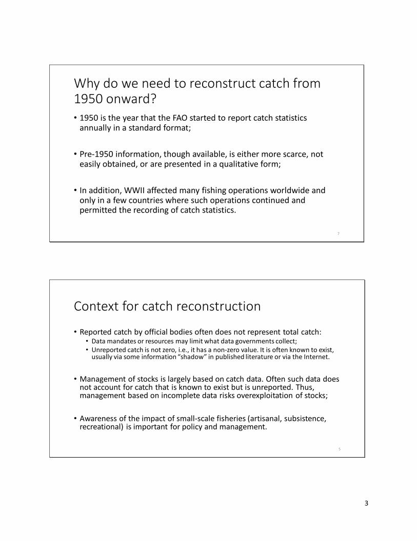
1a. Context for catch reconstructionContext for catch reconstruction;Why do we need a time series?Why do we need to reconstruct catch from 1950 onward?What components do we include in reconstructed catch data?What spatial location data is assigned to catch?What is our catch data used for?
4
3
Why do we need to reconstruct catch from 1950 onward?• 1950 is the year that the FAO started to report catch statistics
annually in a standard format;
• Pre-1950 information, though available, is either more scarce, not easily obtained, or are presented in a qualitative form;
• In addition, WWII affected many fishing operations worldwide and only in a few countries where such operations continued and permitted the recording of catch statistics.
7
Context for catch reconstruction
• Reported catch by official bodies often does not represent total catch:• Data mandates or resources may limit what data governments collect;• Unreported catch is not zero, i.e., it has a non-zero value. It is often known to exist,
usually via some information “shadow” in published literature or via the Internet.
• Management of stocks is largely based on catch data. Often such data does not account for catch that is known to exist but is unreported. Thus, management based on incomplete data risks overexploitation of stocks;
• Awareness of the impact of small-scale fisheries (artisanal, subsistence, recreational) is important for policy and management.
5
4
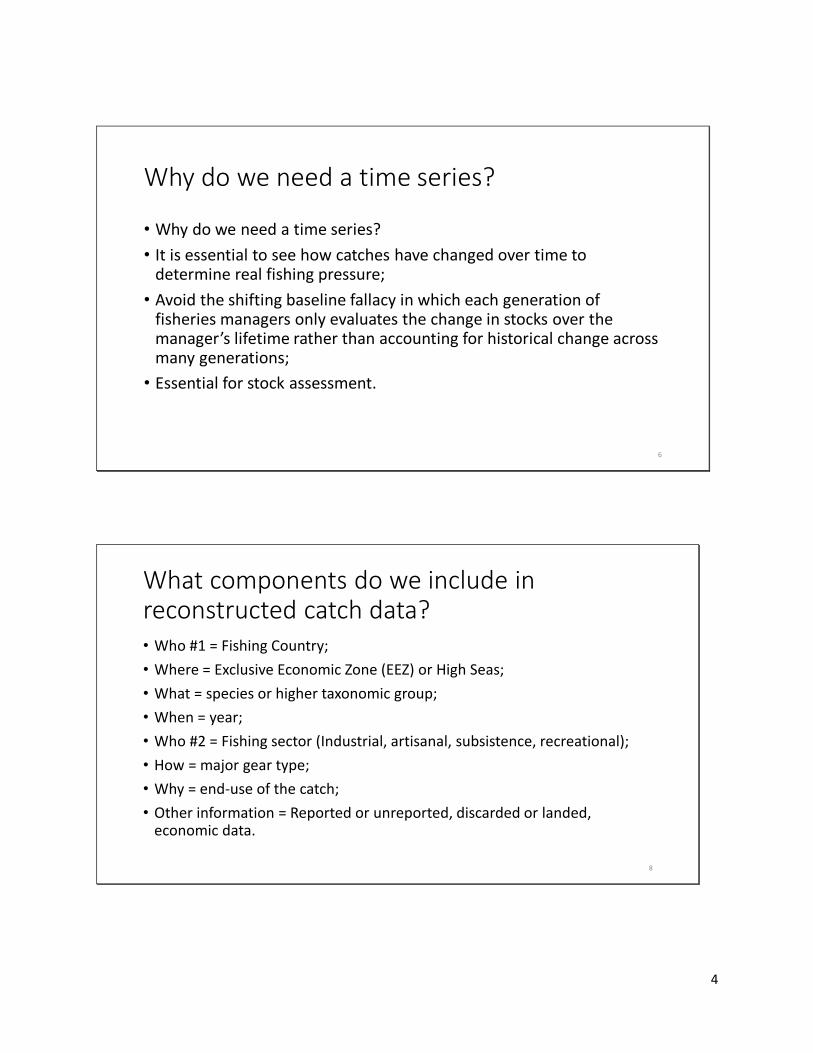
Why do we need a time series?
• Why do we need a time series?• It is essential to see how catches have changed over time to
determine real fishing pressure;• Avoid the shifting baseline fallacy in which each generation of
fisheries managers only evaluates the change in stocks over the manager’s lifetime rather than accounting for historical change across many generations;
• Essential for stock assessment.
6
What components do we include in reconstructed catch data?• Who #1 = Fishing Country;• Where = Exclusive Economic Zone (EEZ) or High Seas;• What = species or higher taxonomic group;• When = year;• Who #2 = Fishing sector (Industrial, artisanal, subsistence, recreational);• How = major gear type;• Why = end-use of the catch;• Other information = Reported or unreported, discarded or landed,
economic data.
8
5
What spatial location data is assigned to catch?• Large Marine Ecosystems;• FAO areas;• EEZs (max. 200 nm from shore):
• Shelf area;• Inshore Fishing Area (50 km offshore or 200 m depth contour) for
inhabited areas with local fisheries.• ICES areas, NAFO areas, CCAMLR areas if applicable;• High Seas areas by FAO area;• Sub regional areas like province/state/island/coast (if applicable);• Locations of coral reefs, seamounts, and primary production.
9
What is our catch data used for?
• Analysis of catch trends over time in globally standardized units;
• Stock Assessment = Bayesian Catch Maximum Sustainable Yield (CMSY)1;
• Stock Status assessment;• Marine Trophic Index;• Multinational footprint;
• Mean temperature of the catch;• Economic analysis;• Spatial mapping of catch;• Outside use of our data by the
United Nations Sustainable Development Goals, Environmental Performance Index, Ocean Health Index, Global Slavery Index, Human Development Index, and Small-Scale Fisheries Records (ISSF).
1 Froese et al. 2017. Fish & Fisheries 18: 506-526 10

6
1b. What is a catch reconstruction?What components of catch are often not reported?Seven basic steps of catch reconstruction;What taxa are included in the reconstructed catch?
11
What is a catch reconstruction?
• Reported
• Catch data reported by a country to an official reporting body (the FAO, ICES, NAFO, CCAMLR) or sometimes nationally reported data for countries with multiple coastlines or islands;
• Reported data has uncertainty associated with it, as most reported data are based on estimations and data collected with measurement and other errors;
• Reconstructed
• Catch data not reported by a country to any official body leading to FAO data, but is known to exist based on national or other data, literature and discussions with local experts;
• Unreported catch estimated based on available information;
• Higher uncertainty than reported catch. However, an estimate with greater uncertainty is better than assuming no catch at all, which results in an erroneous “0” catch in official data.
Total reconstructed catch = reported catch + reconstructed unreported catch
12

7
What components of catch are often not reported?• Sectors: subsistence, recreational and sometimes artisanal, or parts
thereof. Some industrial catch may also be missing due to reporting infrastructure gaps or illegal activities or quota busting;
• Catch types: unregulated fisheries (e.g. subsistence, recreational), or illegal or poached catches or landed by-catch;
• Discarded by-catch;• Official data reported to FAO is also not reported by sector or at the
management-relevant spatial level of EEZs. It is sometimes also reported in broader taxonomic categories than the underlying national or sub-national data. This loss in taxonomic resolution is a substantial degradation of data quality.
13
Seven basic steps of catch reconstruction from Zeller et al. (2016)2
1. Identification, sourcing and comparison of baseline reported catch times series:a. FAO (or other international reporting entities) reported landings data by
FAO statistical areas, fishing country, taxon and year; and b. National and/or sub-national data series by area, taxon, year and any other
available data parameters. Emphasis is placed on capturing total reported catch tonnages in cases of spatial confidentiality rules.
2. Identification of sectors (e.g., subsistence, recreational) or other fisheries components, time periods, taxa, gears etc., not covered by (1), i.e., missing data components. This is conducted via extensive literature searches and consultations with local experts.
2 Zeller et al. 2016. Marine Policy 70: 145-152 14
8
Seven basic steps of catch reconstruction from Zeller et al. (2016)2
3. Sourcing of available alternative information and secondary data sources on missing components identified in (2), via extensive searches of the literature (peer-reviewed and grey, both online and in hard copies) and consultations with local experts. Information sources can also include social science studies (anthropology, economics, etc.), reports, colonial archives, data sets and expert knowledge;
4. Development of data ‘anchor points’ in time for each missing data component, and careful expansion of anchor point data to country-wide catch estimates.
2 Zeller et al. 2016. Marine Policy 70: 145-152 15
Seven basic steps of catch reconstruction from Zeller et al. (2016)2
5. Interpolation for time periods between data anchor points, either linearly or assumption-based for commercial fisheries, and generally via per capita (or per-fisher) catch rates for non-commercial sectors. Important societal and socio-economic (e.g., wars, economic collapse, civil unrest) and environmental impacts (e.g., tsunamis, destructive storms) to be taken into account;
6. Estimation of total catch times series, combining reported catches (1) and interpolated, country-wide expanded missing data series of unreported catches (5);
7. Quantifying the uncertainty associated with each reconstruction (see module 4c).
2 Zeller et al. 2016. Marine Policy 70: 145-152 16

9
What taxa are included in the reconstructed catch?INCLUDED• Marine, brackish, and
anadromous/catadromous fishes and invertebrates;
• Unwanted discard-only taxa;• Taxa used for production of bait or
fishmeal/oil only;• Roe/shark fins/conch meat/etc.
converted to whole weight of individual taxa (including shell weight);
NOT INCLUDED• Aquaculture (*separate
mariculture database);• Freshwater taxa;• Taxa for aquarium trade or
“curiosities”/jewelry/decoration purposes;
• Reptiles, marine mammals, plants/algae, corals; and
• Portion of catch and release fisheries where individuals survived.
17
1c. Data layers and database process to map catchProcess from raw catch data to spatially allocated catch and to web data;What categories are essential for mapping?Fishing outside the home EEZ;Industrial catches of tunas and other large pelagic and associated by-catch and discards;Data Layer 3 species.
18

10
Process of catch from raw data to web data
Raw catch data in Excel working files in database format INT DB– integration database
Merlin – processing database. This is where catch is spatially allocated using other information
Web DB – spatially allocated web database
Database that supports web products that are also available for external download.
19
Mapping catch data: the Geospatial database
• Global oceans subdivided into 150,000 sea-ice free GIS grid cells of ½ degree Latitude by ½ degree Longitude resolution;
• Each grid cell has numerous data parameters associated with it:
• % water versus land;• Mean water depth;• Broad habitat types, e.g., % of seamounts, % of
estuaries, % of coral;• Affiliation with other geospatial entities, such as EEZs,
FAO area, LMEs, Marine Ecoregions, climatic zones etc.
20

11
What categories are essential for mapping?
• Taxon3;• Fishing country ;• EEZ, FAO area;
• Any catch pre-assigned to areas outside an EEZ is allocated to half degree cells based on the area assigned, the fishing access database, and the taxon distribution database and presented on the web in map and graph form.
www.seaaroundus.org
3 The term taxon is applied to species or species groups (genus, family, order, class or ‘nei’ 21
Domestic fishing inside the home EEZ
Data Layer 1• Fishing by a fishing country inside its own home EEZ is assigned to
layer 1. This is the core product of most catch reconstructions;• Catch can be reported or reconstructed landings and/or discards;• Can be industrial, artisanal, subsistence and recreational sectors;• Can be in one of several home EEZs “owned” by the country in
question, e.g., France’s EEZ in Atlantic Ocean versus Mediterranean Sea. These are usually derived from separate reconstructions, as reconstructions are based on EEZs.
22

12
Fishing outside the home EEZ
Data Layer 2• Fishing by a fishing country outside their home EEZ is assigned to layer 2;• Catch can be reported or reconstructed landings and/or discards;• All fishing outside a home EEZ is consider to be from the industrial sector
only;• Fishing can be in another country’s EEZ, a high seas area, or a general
“outside of EEZ” if unknown:• “Outside of EEZ” is allocated to EEZs or high seas areas based on:
FAO area + fishing access data + taxon distribution
23
Industrial catches of tunas and other large pelagic taxa, and associated bycatch and discardsData Layer 3• Tuna Regional Fisheries Management Organizations (RFMOs) provide catch data for tuna
and other large pelagic species, and some information on associated bycatch/discards;• Non-industrial components (i.e., artisanal), if reported by RFMOs, are excluded from
layer 3, but harmonized with layer 1 and 2 data whenever possible. Conservative approach, to avoid possibility of double counting;
• Some RFMO data subsets (not all catch) are available at a variety of higher spatial resolution than only FAO area (i.e., 1ox1o – 20ox20o “tuna cell” resolution);
• This data is pre-processed to “tuna cells”3 and added into the Sea Around Us spatial allocation process separately from layer 1 and 2 reconstructed data;
• Thus, such industrial tuna catches need to be excluded from national or FAO reported baseline data (and associated by-catch and discard estimations) during reconstruction of layer 1 and 2 data, or they need to be marked as layer 3 in final dataset for removal by allocation data team from layer 1 and layer 2 data to avoid double counting.
4 Le Manach et al. 2016. Chapter 3 in: Global Atlas of Marine Fisheries: A critical appraisal of catches and ecosystem impacts; and Coulter et al. in review
24

13
Data Layer 3 species5
5Does not include bycatch species 25
2. Searching for informationWhat type of information is helpful for reconstructing catch?Common information used;Where to find information?Uncertainty in sources and methods;Is the information representative?Apparent seafood consumption rates.
26
14
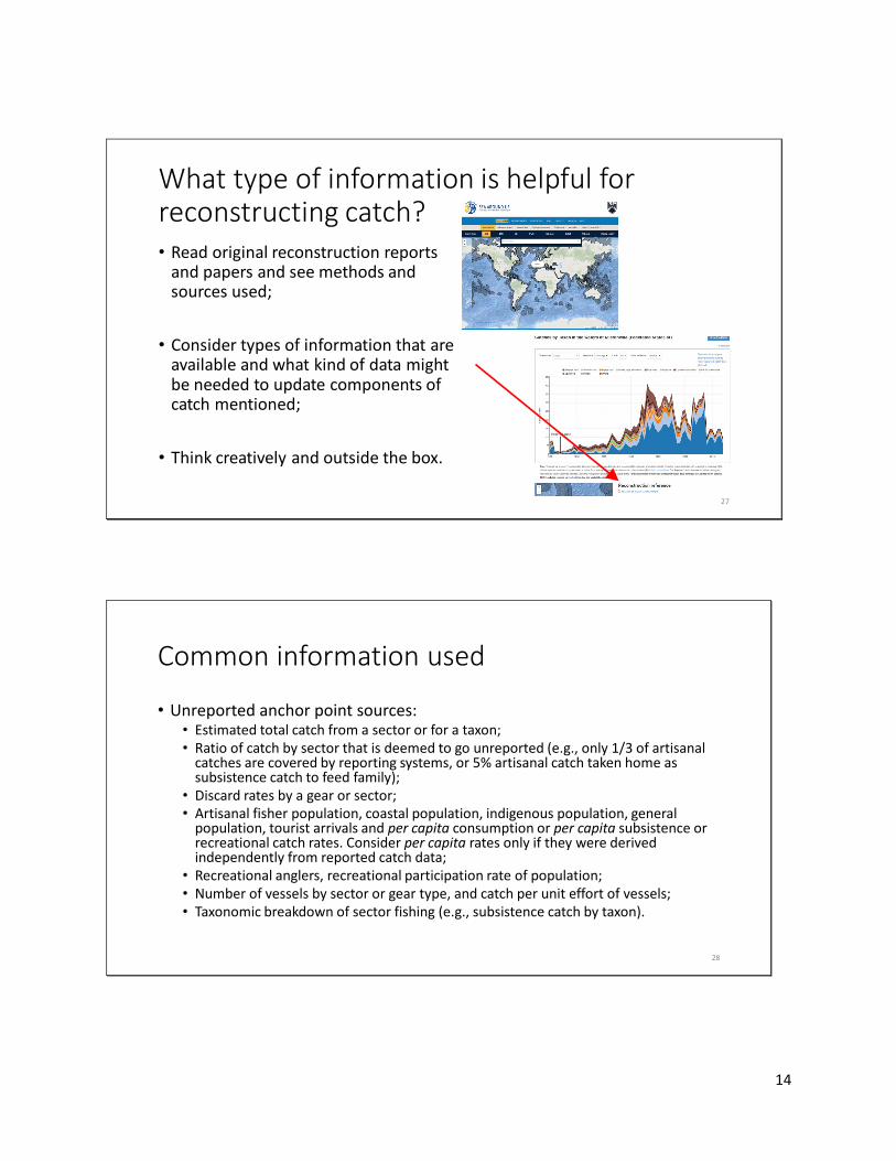
What type of information is helpful for reconstructing catch?• Read original reconstruction reports
and papers and see methods and sources used;
• Consider types of information that are available and what kind of data might be needed to update components of catch mentioned;
• Think creatively and outside the box.
27
Common information used
• Unreported anchor point sources:• Estimated total catch from a sector or for a taxon;• Ratio of catch by sector that is deemed to go unreported (e.g., only 1/3 of artisanal
catches are covered by reporting systems, or 5% artisanal catch taken home as subsistence catch to feed family);
• Discard rates by a gear or sector;• Artisanal fisher population, coastal population, indigenous population, general
population, tourist arrivals and per capita consumption or per capita subsistence or recreational catch rates. Consider per capita rates only if they were derived independently from reported catch data;
• Recreational anglers, recreational participation rate of population;• Number of vessels by sector or gear type, and catch per unit effort of vessels;• Taxonomic breakdown of sector fishing (e.g., subsistence catch by taxon).
28
15
Where to find information?
• Scientific literature;• National Fisheries Ministry website;• National statistical office (census, etc.);• Regional fisheries management bodies and working groups, including FAO;• NGO/non-profit reports and stock assessment working groups;• Socioeconomic studies (GDP, changes in meat consumption, subsistence);• Google news for country;• Google specific sectors or fishing statistics using the primary language of
country and see what sources come up;• Grey literature (trip advisor, tourism websites);• Communication with local experts.
29
Uncertainty in sources and methods
• Some sources of data come from ‘less certain’ sources of information. Keep track of the level of trust in such data sources for later use in estimating the uncertainty of reconstructed data (see module 4c);
• In some countries, there may not be a lot of information from official sources. This might mean that more grey literature sources and assumptions are required to reconstruct missing components of the catch, thus increasing the level of uncertainty;
• Such information is still useful. The uncertainty score for the data and methods per sector (see module 4c) is used to reflect the quality of such information.
30
16
Is the information found representative?
• Consider whether the study accurately reflects the area, sector or fisheries component to be represented;
• What assumptions would be made to use it?
• A study of one port or landing site may not reflect an entire country;• A study of seafood consumption in rural coastal regions of the country may
not represent the seafood consumption rate of urban populations;• A study of participation in recreational fishing in a country may include
freshwater sport fishing.
31
Apparent seafood consumption rates
• FAO (and some other sources) provides estimates of per capita seafood consumption rates based on total population and catch reported to FAO;
• Per capita seafood consumption rates derived from reported catch is known as apparent seafood consumption;
• For the purposes of reconstructions in cases where we are trying to derive total catch based on consumption rates (e.g., subsistence fisheries), we need estimates of per capita seafood consumption that is derived independently from reported catch data;
• Estimating catch using apparent seafood consumption rates results in a circular logic and needs to be avoided.
32

17
3. Identification and comparison of reported data3a. Adding resolution to reported catch data;3b. Checking for retroactive changes to reported data;3c. Working with national data;3d. Reported data from ICES, NAFO, or CCAMLR;3e. Identifying improvements to reporting;3f. Handling of new taxonomic categories in reported data;3g. Falsification of reported catch data.
33
3a. Adding resolution to reported catch dataReported baseline;Limitations of FAO reported data;Reported baseline resolution;Reported baseline and layer 3;Reported baseline and multiple FAO areas.
34

18
Reported baseline
• All maritime countries that are FAO member countries report catch to the FAO annually upon request, or their catches are estimated by FAO in cases of non-reporting (currently over 25% of countries do not report annually). The FAO estimation method is not publicly documented.
• The FAO compiles this information and makes it available for download in standardized units and species names.
35
Limitations of FAO reported data
• FAO reported as caught from broad ocean areas (FAO statistical areas);
• Often reported in broad taxonomic groups (e.g., Marine fishes nei6);
• Not separated by fishing sector (industrial, artisanal etc.);
• Consists of landed catches only, discarded catches are explicitly excluded from FAO data.
www.fao.org
6not elsewhere identified 36

19
Reported baseline resolution• We take the reported
information from FAO and:• Allocate reported catch by FAO
area to EEZs and/or high seas;• Provide more resolution to
taxonomic information for FAO taxonomic groups based on literature information;
• Allocate FAO data to the fishing sectors that are catching each taxon.
FAO data
Sea Around Us reported data
37
Reported baseline and layer 3
• Layer 3 (= industrial tuna landings and associated bycatch and discards) is accounted for by a separate process (see section 1: slides 17-18). Thus, it is NOT part of the raw catch sets from reconstructions (but it is integrated and allocated to ½ degree cells and thus part of the data accessible from the web database);
• This is marked as layer 3 in the layer column or removed from the final raw reconstructed catch data file so as to avoid double-counting.
38

20
Reported baseline and multiple FAO areas
• Some countries report catch for multiple FAO areas. This may be because a country has EEZs in more than one FAO area (e.g., India) and/or a country is fishing in other ocean basins using distant-water fleets;
• A set of methods may include some or all of the catch reported to FAO for all of the FAO areas where that country is fishing;
• Some reconstructions will cover any/all fishing countries within that country’s EEZ, thus producing not only layer 1 data, but also components of layer 2. Or they might cover some/every EEZ where a particular fishing country is fishing or some combination in order to cover all catch that is reported;
• Only update the FAO area data included in a particular reconstruction methods unless a country is newly fishing in an FAO area and is not covered elsewhere or previously.
39
3b. Checking for retroactive changes to reported dataRetroactive changes to reported baseline;Compare reported baseline in reconstruction with FAO data.
40

21
Retroactive changes to reported baseline
• FAO releases annual updated catch statistics. Sometimes, reported catch by species is revised for years earlier in the time period based on updated information;
• Check for these retroactive changes by comparing, for each FAO area separately, the totals per taxon per year of the last FAO data version used in the Sea Around Us Integration database and the most recent version of the updated FAO database. Look for which FAO taxon names cause the difference:
• Are there new taxa added or were taxa disaggregated or pooled between FAO data versions?
• Are there retroactive changes to catch amounts in earlier years?
41
Compare reported baseline in reconstruction with FAO data• Compare versions of FAO data to
identify new taxonomic groups and retroactive changes to catch;
• Then compare FAO data to the reported landings in the reconstructed database to identify where retroactive changes may be required:
• Include only same taxa (exclude layer 3) and area when comparing;
• Use the column ‘original_fao_name’ to compare totals per FAO taxonomic group.
42
22
3c. Working with national dataWhy is national data sometimes used in place of FAO?Why national data may not be equal to reported FAO data?Comparing national data with FAO.
43
Why is national data sometimes used in place of FAO?• If and only if national data is approximately equivalent to the data
reported to FAO, national data is sometimes used in place of FAO to reflect higher resolution in national data such as:
• Subareas – coasts, provinces, states, islands;• Sectors catching reported data;• Catch reported by gear; and• Increased taxonomic resolution in nationally reported data.
44

23
Why national data may not be equal to reported FAO data?• Errors in data transfer as catch is combined and assembled from various
locations/reporting systems may result in missed catch or different identification of taxa;
• Different units (product weight versus whole weight, pounds vs tonnes, number of animals instead of whole weight etc.);
• One source may include catches landed in a country by foreign fleets, and report these as domestic catches;
• FAO receives and harmonizes various data sources, e.g., from tuna RFMOs. Some of these RFMO data may not be in the data reported by national authorities to FAO;
• FAO might have used conversions from product weight to whole weight etc.
45
Comparing national data with FAO
FAO > National
If FAO data is substantially larger than nationally reported data for the same area, after accounting for tuna RFMO data, Sea Around Us assumes that national reported data largely reflects catch within its home EEZ, unless information exists to the contrary. This key assumption is crucial to verify during reconstruction. Such excess catch reported to FAO in a given FAO area is assumed to be taken outside of the home EEZ, i.e., becomes part of layer 2 data.
National > FAO
If national data is larger than reported to FAO, Sea Around Us considers the excess catch to be unreported catch with respect to international accounting via FAO. This needs close attention and verification during reconstruction. Yes, it’s reported nationally, but not internationally reported to officially recognized inter-governmental bodies of the UN, namely FAO.
46

24
3d. Reported data from ICES, NAFO, or CCAMLRDifferences when baseline area from ICES, NAFO, CCAMLR data?
47
Differences when baseline are from ICES, NAFO, CCAMLR data?• Include catch reported to smaller spatial subareas other than the FAO
fishing areas. These subareas must be included in the corresponding column of the raw catch data table to contribute to the mapping process:
• CCAMLR – catch data recorded for Southern Antarctic Ocean;• Discards may be reported;• Older data may not be presented by calendar year, but by fishing season (July-June). This
needs converting.• NAFO – Northwest Atlantic Ocean:
• Catch reported at statistical sub-areas, e.g., ‘Area 6b’;• Some areas may include ICES and NAFO areas.
• ICES – catch data and stock assessment from Northeast Atlantic Ocean:• Catch reported at statistical sub-areas of ICES areas, e.g., ‘27.xiv.b2’;• Sometimes reported as sub-area ‘n-k’ (not-known). Must be tracked to get total catch.
48
25
3e. Identifying improvements to reportingHow to identify improvements to reporting;Presentist bias.
49
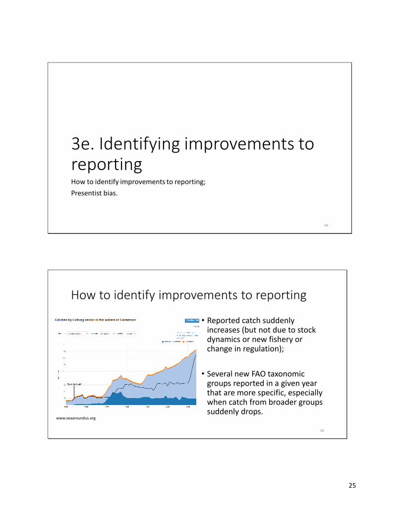
How to identify improvements to reporting
• Reported catch suddenly increases (but not due to stock dynamics or new fishery or change in regulation);
• Several new FAO taxonomic groups reported in a given year that are more specific, especially when catch from broader groups suddenly drops.
www.seaaroundus.org
50

26
Presentist bias
• Improvements in catch reporting due to improved data collection systems lead to rapid increases in reported catches without corresponding past catches being fully corrected retroactively;
• Problem: catch does not reflect true exploitation of stocks and contributes to shifting baselines.
Zeller D and Pauly D (2018). The ’presentist bias’ in time-series data: implications for fisheries science and policy. Marine Policy 90: 14-19. 51
3f. Handling of new taxonomic categories in reported data
52
27
How to handle new FAO taxonomic categories introduced to reported data1. Has this species or a higher taxonomic category (e.g., family) been
fished previously? Has the species/broader group been reported previously? Has catch for this higher group dropped?a. If yes, likely need to adjust taxonomic breakdowns. See module 5.
2. Is this a new fishery? Is this a species that could not have been accessed previously due to technological requirements, etc.?a. If yes, include the species on the year the fishery began.
53
3g. Falsification of reported catch data
54

28
How to identify falsification of data• Political pressure or standard government
policies can cause officials to deliberately or accidentally falsify catch data to meet catch targets, e.g., China and Myanmar:
• Catch increases exponentially from year to year.
• In cases where data falsification occurs, total catch must be reconstructed from available information and an adjustment factor is applied to reported catch to lower catch to the reconstructed amount.
Watson R and Pauly D (2001) Systematic distortions in world fisheries catch trends. Nature 414: 534-536.
55
4. Methods of reconstructing catch by sector
4a. General approaches to catch reconstruction by sector;4b. Disaggregation of catch by area, reporting status, taxa and gear;4c. Documentation of methods.
56

29
4a. General approaches to catch reconstruction by sectorHow to approach catch reconstruction;Two major approaches reconstructing sectors;Interpolating between anchor points;Common methods by sector.
57
How to approach catch reconstruction• Always reconstruct FAO areas, fishing entities, EEZs, sectors, subsectors
separately. Pivot tables and pivot table graphs in excel can help visualize data and are a crucial tool.
58
30
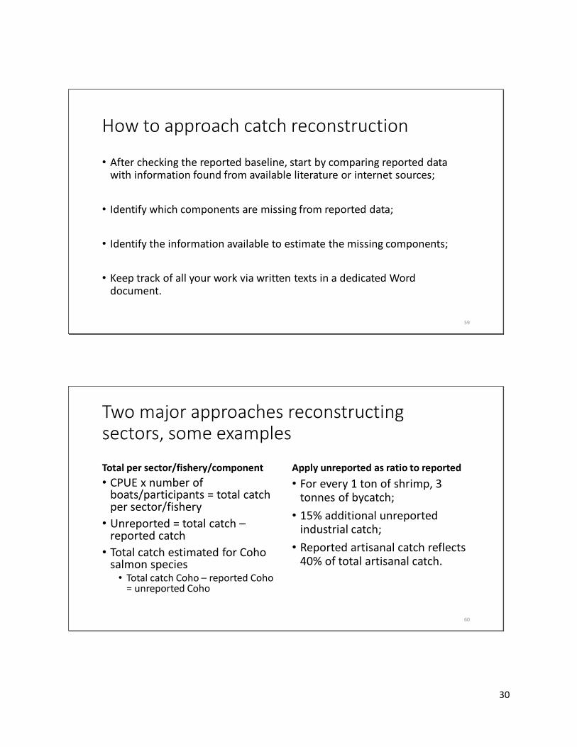
How to approach catch reconstruction
• After checking the reported baseline, start by comparing reported data with information found from available literature or internet sources;
• Identify which components are missing from reported data;
• Identify the information available to estimate the missing components;
• Keep track of all your work via written texts in a dedicated Word document.
59
Two major approaches reconstructing sectors, some examples
Total per sector/fishery/component• CPUE x number of
boats/participants = total catch per sector/fishery
• Unreported = total catch –reported catch
• Total catch estimated for Coho salmon species
• Total catch Coho – reported Coho = unreported Coho
Apply unreported as ratio to reported• For every 1 ton of shrimp, 3
tonnes of bycatch;• 15% additional unreported
industrial catch;• Reported artisanal catch reflects
40% of total artisanal catch.
60

31
Interpolating between anchor points
• Anchors may not be available for every year;• The slope between anchor points can be assumed to reflect the most likely change when
additional information is not available;• Interpolations need to take key socio-economic (economic collapse = increased subsistence
demand), political (civil war) and environmental effects (tsunami) into account.
0
10
20
30
40
50
60
70
2006 2007 2008 2009 2010 2011 2012 2013 2014 2015 2016
Per Capita Consumption Rate (kg/person)
Per Capita Consumption Rate (kg/person)
Total domestic catch = Population x per capita consumption rate
Interpolation
61
Common methods: Industrial fisheries
• Most likely sector to have reported data;• Includes catch by large-scale commercial vessels;• Unreported industrial landings often calculated either by:
• Ratio of unreported catch to reported landings of given taxa or fishery;• Total catch for a taxon caught by industrial gears reported by the country
minus FAO reported catch for that taxon;• Catch per unit effort (CPUE) applied to number of vessels and associated
effort.
62
32
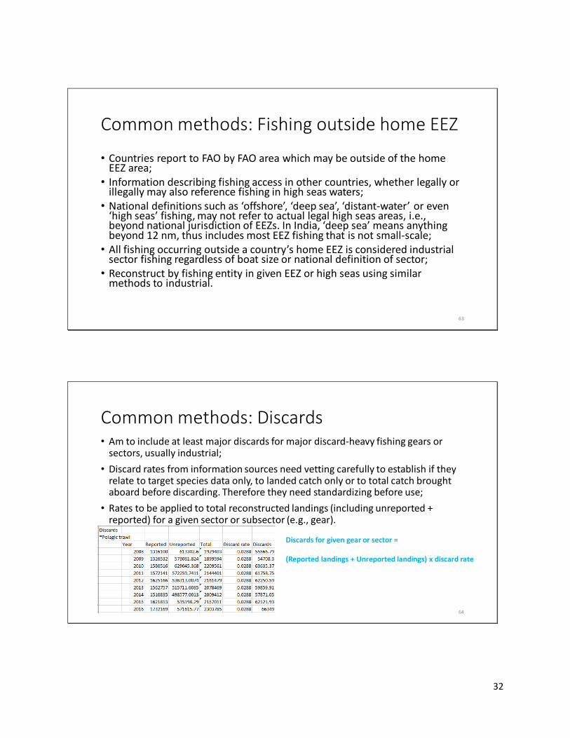
Common methods: Fishing outside home EEZ
• Countries report to FAO by FAO area which may be outside of the home EEZ area;
• Information describing fishing access in other countries, whether legally or illegally may also reference fishing in high seas waters;
• National definitions such as ‘offshore’, ‘deep sea’, ‘distant-water’ or even ‘high seas’ fishing, may not refer to actual legal high seas areas, i.e., beyond national jurisdiction of EEZs. In India, ‘deep sea’ means anything beyond 12 nm, thus includes most EEZ fishing that is not small-scale;
• All fishing occurring outside a country’s home EEZ is considered industrial sector fishing regardless of boat size or national definition of sector;
• Reconstruct by fishing entity in given EEZ or high seas using similar methods to industrial.
63
Common methods: Discards• Am to include at least major discards for major discard-heavy fishing gears or
sectors, usually industrial;• Discard rates from information sources need vetting carefully to establish if they
relate to target species data only, to landed catch only or to total catch brought aboard before discarding. Therefore they need standardizing before use;
• Rates to be applied to total reconstructed landings (including unreported + reported) for a given sector or subsector (e.g., gear).
Discards for given gear or sector =
(Reported landings + Unreported landings) x discard rate
64

33
Common methods: Artisanal
• This sector is the next most likely to have reported data;• Sea Around Us defines this as catches by smaller, less capital intensive vessels, or fishing
from shore. Primary purpose of artisanal fishing is the sale of the majority of the catch;• Use primarily passive or static fishing gears;• Artisanal fisheries only occur within a country’s home EEZ;• Trawl fisheries and any gear dragged across sea floor or intensively through water
column using engine power are always considered industrial by Sea Around Us, no matter the vessel size;
• Unreported artisanal landings often calculated either by:• Ratio of unreported catch to reported landings of given taxon, gear or fishery;• Total catch for a taxon caught by artisanal gears reported by the country minus FAO reported catch
for that taxon;• Catch per unit effort (CPUE) applied to number of vessels or number of fishers and associated
effort measure.
65
Common methods: Subsistence
• Take home catch from commercial fisheries (usually artisanal only) for family consumption:
• % take home catch x commercial (artisanal) catch;• Per capita take home catch x number of commercial (artisanal) fishers.
• Consumption or catch rate:• Per capita subsistence seafood consumption rate x coastal or total population;• Per subsistence fisher catch rate x population participating in subsistence
fishing;• Population may be for specific select group (urban, rural, particular islands,
indigenous groups, coastal population, etc.).
66
34
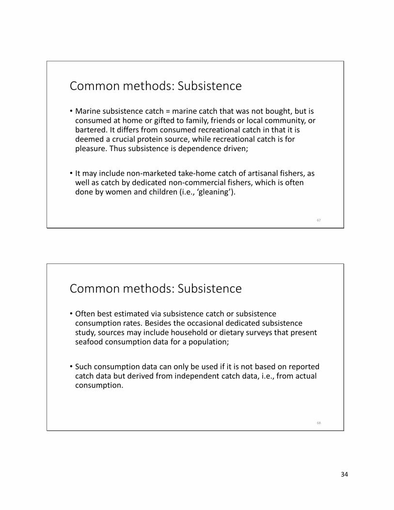
Common methods: Subsistence
• Marine subsistence catch = marine catch that was not bought, but is consumed at home or gifted to family, friends or local community, or bartered. It differs from consumed recreational catch in that it is deemed a crucial protein source, while recreational catch is for pleasure. Thus subsistence is dependence driven;
• It may include non-marketed take-home catch of artisanal fishers, as well as catch by dedicated non-commercial fishers, which is often done by women and children (i.e., ‘gleaning’).
67
Common methods: Subsistence
• Often best estimated via subsistence catch or subsistence consumption rates. Besides the occasional dedicated subsistence study, sources may include household or dietary surveys that present seafood consumption data for a population;
• Such consumption data can only be used if it is not based on reported catch data but derived from independent catch data, i.e., from actual consumption.
68

35
Common methods: Subsistence
• Guard carefully against inclusion of freshwater catches, as sometimes freshwater fish are included in the category ‘fish and invertebrates’ in consumption data for a country that is not specific to marine fisheries;
• Thus, such data might differ from a marine fish consumption rate;• Estimate a marine consumption rate from overall fish consumption
rate if information for freshwater/aquaculture production of fish and invertebrate and import/export information. Calculate subsistence once the commercial sectors are subtracted.
69
Common methods: Subsistence
• In practice, this is often not possible, and if no dedicated subsistence studies exist for the country, area or region, we use conservative assumptions. Derive conservative subsistence catch rates (e.g., g/day per coastal population) or assume a fraction of total household consumption being marine subsistence for total coastal population;
• Use the coastal population databases from, e.g., the World Bank.
70
36
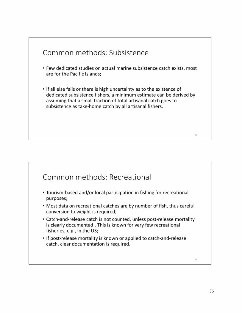
Common methods: Subsistence
• Few dedicated studies on actual marine subsistence catch exists, most are for the Pacific Islands;
• If all else fails or there is high uncertainty as to the existence of dedicated subsistence fishers, a minimum estimate can be derived by assuming that a small fraction of total artisanal catch goes to subsistence as take-home catch by all artisanal fishers.
71
Common methods: Recreational
• Tourism-based and/or local participation in fishing for recreational purposes;
• Most data on recreational catches are by number of fish, thus careful conversion to weight is required;
• Catch-and-release catch is not counted, unless post-release mortality is clearly documented . This is known for very few recreational fisheries, e.g., in the US;
• If post-release mortality is known or applied to catch-and-release catch, clear documentation is required.
72

37
Common methods: Recreational
• Note: subsistence and recreational catch overlap as fishers consume recreational catch. Careful not to double-count;
• There is also a gradual shift over time from subsistence fishing to recreational fishing with increased economic development in a country. This applies especially to emerging economies, with increasing disposable incomes and reduced reliance on subsistence;
• On the other hand, economic collapses and political turmoil that leads to strong downturns or collapse of economies may lead to increased subsistence focus and increased subsistence catch.
73
Common methods: Recreational
Recreational catch is often estimated using the following methods:• Tourism arrivals x per capita participation rate in recreational fishing7
x per capita recreational catch = recreational catch• Number of recreational licenses x per capita recreational catch =
recreational catch• One of the methods above for total recreational catch targeted x % catch and release x % mortality from catch and release = recreational catch
7 If no location specific study exist, consider Cisneros-Montemayorand Sumaila (2010) Journal of Bioeconomics 12: 245-268. 74

38
4b. Disaggregation of catch by area, reporting status, taxa and gear Disaggregate catch using breakdowns;Disaggregate catch: FAO area, EEZ, subareas;Disaggregate catch: Reported vs Unreported;Disaggregate catch: Reported catch by sector.
75
Disaggregate catch using breakdowns
• Each row of data in the final reconstructed data set that will be integrated into the Sea Around Us Integration database represents unique information. Each component of catch needs a separate row;
• Some reconstructions make use of the notes column to help keep track of separate subcomponents.
76

39
Disaggregate catch: FAO area, EEZ, subareas
www.seaaroundus.org 77
Disaggregate catch: Reported vs Unreported
• Depending on the methods used, in general:
1. Separate reported catch data into sectors and then add on unreported components to each sectors; or
2. Separate total reconstructed catch into reported and unreported components by sector. ‘Total catch – Reported = Unreported’
78

40
Disaggregate catch: Reported catch by sector
• Reported catch allocated to sectors based on species caught or other relevant data for countries, such as data on catch by gear type;
• This method is used when certain species are entirely or mainly caught by one sector;
• Data of national catch by sector may be helpful for allocating the reported tonnage for a species by sector;
• If all species are caught by multiple sectors, the overall proportion between sectors to split total reported catch between sectors might be the best option.
79
Disaggregate reported catch: original FAO name
• Total by FAO taxon name must match what is reported for that category to FAO or other reporting body.
80

41
Disaggregate reported catch: taxonomic breakdowns• Broad taxonomic groups at family or higher levels are disaggregated
where possible based on information from literature.
Taxonomic breakdown
FAO name “Penaeus shrimps nei” disaggregated by species
81
Disaggregate unreported catch: taxonomic breakdowns
Unreported components taxonomic breakdown may be based on: a. The reported species
breakdown;b. Taxonomic breakdown
derived from catch by species (in weight) anchors in literature.
82

42
Disaggregate catch: original taxon name
• More specific taxonomic information may be provided in the column ‘original_taxon_name or taxon_notes’ if there is no available distribution at species level;
• If the taxon name has been updated, the previous name may be maintained in the column ‘original_taxon_name’;
• These additional information regarding catch must be maintained.
83
Disaggregate catch: industrial gear
• Tim Cashion produced a report5 detailing his sources and assumptions for gear;
• Catch for individual taxa were assigned a gear breakdown for each EEZ based on gear data for a country’s catch if available or most likely gears used;
• Unless other information is available, maintain gear breakdown by taxon as for previous years.
5 Cashion et al. (2018) Fisheries Research 206: 57-64. 84

43
Disaggregate catch: artisanal gear
• Artisanal gear was assigned to catch using a regional breakdown8:
• The top 3 artisanal catch producing countries per geographic region were analysed and assigned gear types in order to represent artisanal gear breakdown by taxon in the region. This average artisanal gear breakdown was applied across countries in that geographic region;
• Again, unless other information is available, maintain the species gear breakdown for artisanal catch at the last year’s data.
8 Cashion et al. (2018) Fisheries Research 206: 57-64.85
Disaggregated catch in database format
• Check that totals per year per component of catch in the final database file as they are in the working-files used for calculations;
• Plot totals by area and by sector and by taxon to check for catch patterns that raise red flags;
• These steps are part of basic data back checking.
86

44
Assumptions that can be made in updating catch in the absence of other data• Taxa are caught by the sector they have been assigned to in a
previous year. If these are exclusively caught by industrial sector and there is nothing that suggests that a new artisanal fishery is now catching this taxon, assume that it is still exclusively caught by industrial sector. If caught by two or more sectors and not proportioned out based on reconstructed total catch by sector, assume the same proportion of reported catch per sector;
• If catch trend over time is not increasing over the last few years, use the proportion of unreported components to reported components as described in the methods when methods use a ratio.
87
Assumptions that can be made in updating catch in the absence of other data• The same methods as the last year calculated in the original report as
long as information is updated (e.g., population/boats/fishers/rates);
• Ensure that the trend in catch is maintained or have information to explain why that trend changed;
• The taxonomic breakdown for components and gear by taxa breakdowns are the same as in the last year with data unless otherwise specified information.
88
45
4c. Documentation of methods
89
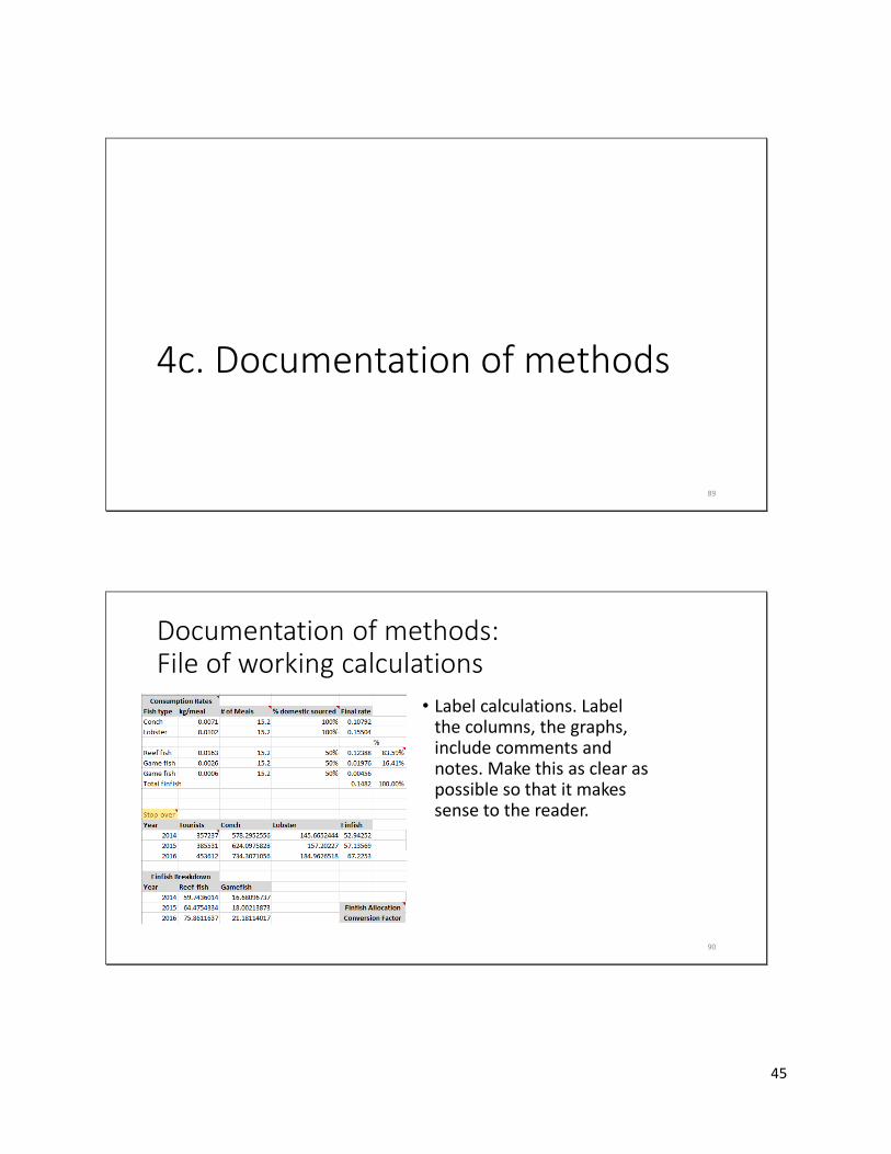
Documentation of methods: File of working calculations
• Label calculations. Label the columns, the graphs, include comments and notes. Make this as clear as possible so that it makes sense to the reader.
90

46
Documentation of methods: File of working notes• A word document that describes methods followed by each
component of catch, including whether retroactive changes were made, assumptions made, etc. Can be in bullet point format, as long as this is understandable to the reader, i.e., the next person who will update the reconstructions;
• Document also needs to clearly describe, list and reference all data and information sources used, especially any new and updated data and information sources;
• Local expert sources and contacts that contributed or answered queries should also be listed, complete with contact details, affiliations and position.
91
Documentation of methods: Addendum• An updated addendum that describes the methods used for this update of
the reconstruction, from the last year of reconstruction or review to current year of data used, e.g., from 2011-2016 (*incorporate the previous addendum and/or update it if new methods are used). This will be published on the Sea Around Us website;
• Cite sources;
• Plot catch from 2000 onward or earlier if retroactive changes were made.
92

47
Documentation of methods: Uncertainty scores9
Scores assigned per sector (industrial, artisanal, subsistence, recreational) and for discarding, per EEZ, per 20 year periods:
1950-19691970-19891990-20092010-2029
Table S1. Scoring system for deriving uncertainty ranges for the quality of time series data of reconstructed catches.
Score +/-%a Corresponding IPCC criteriab
4 Very high 10 High agreement & robust evidence
3 High 20 High agreement & medium evidence or medium agreement & robust evidence
2 Low 30 High agreement & limited evidence or medium agreement & medium evidence or low agreement & robust evidence.
1 Very low 50 Less than high agreement & less than robust evidencea Percentage uncertainty derived from Monte-Carlo simulations.b “Confidence increases” (and hence percentage ranges are reduced) “when there are multiple, consistent independent lines of high-quality evidence”.
9See Supplementary Materials in Zeller et al. (2016). Marine Policy 70:145-152. 93
Documentation of methods:Checklist
1) Final database formatted file;2) Working calculations file (annotated);3) Working notes on data, methods and assumptions:
• Include uncertainty scores per sector and discards, per time period.
4) Addendum of methods including retroactive changes made;5) Saved copies of any sources including screenshots of webpages.
94

48
5. Trouble-shooting
95
Troubleshooting
• Every reconstruction is different;
• New information can mean retroactive changes need to be made. Determine how far back necessary to avoid presentist bias;
• Lack of available new/recent information can make updating difficult and requires more assumptions.
96

49
Troubleshooting: Unlikely catch patterns• Spikes, crashes, or unlikely rises;• Spikes:
• Applying a rate to a catch that spikes or rapidly rises will magnify in unreported. May or may not be accurate.
• Crash/no longer reported:• Research whether fishing still occurs
and reconstruct as unreported if so.• Unlikely steep rise in catch:
• Ex: Methods driven by population demand or tourist demand for low resilient species can be unlikely. May need alternative method;
• Could indicate major change in data system in a country – requires detailed investigation.
97
Improved reporting affects unreported catch• If reporting has improved, carry forward method should not employ an unreported rate.
• Requires examination for potential presentist bias versus actual fisheries changes (e.g., foreign reflagging)
98
50
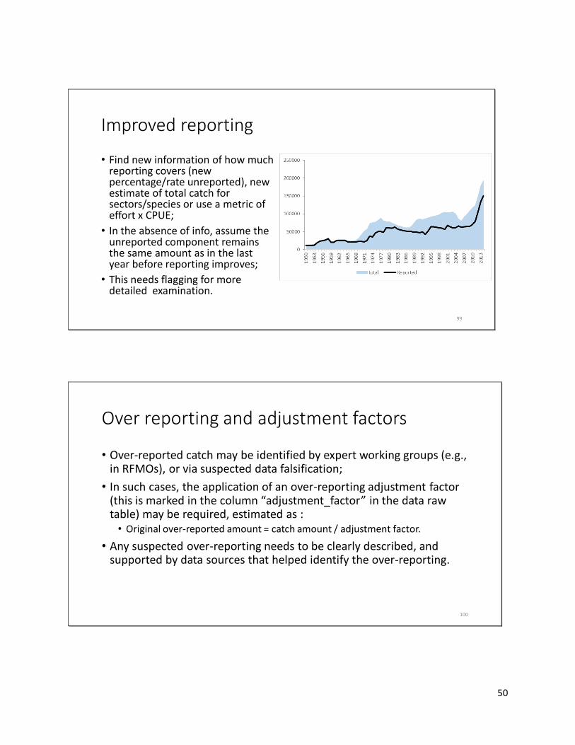
Improved reporting
• Find new information of how much reporting covers (new percentage/rate unreported), new estimate of total catch for sectors/species or use a metric of effort x CPUE;
• In the absence of info, assume the unreported component remains the same amount as in the last year before reporting improves;
• This needs flagging for more detailed examination.
99
Over reporting and adjustment factors
• Over-reported catch may be identified by expert working groups (e.g., in RFMOs), or via suspected data falsification;
• In such cases, the application of an over-reporting adjustment factor (this is marked in the column “adjustment_factor” in the data raw table) may be required, estimated as :
• Original over-reported amount = catch amount / adjustment factor.
• Any suspected over-reporting needs to be clearly described, and supported by data sources that helped identify the over-reporting.
100

51
Improving taxonomic breakdownsOver time, catch reporting systems have improved to include greater portions of catch but also to identify catch to more specific taxonomic groups;
Species are not always reported earlier in time series and are not always disaggregated retroactively;
If this is not a species that has never been targeted, try to match with catch for family or broader taxonomic group.
101
Improving taxonomic breakdowns
1) Identify the family of each species and sort by sector, reporting status, catch type and family to identify the species to use for disaggregating a broader category into for earlier years;
2) Take the average proportion of species for the first five years of detailed reporting out of the catch for this family if information is not available to disaggregate;
3) Apply proportions to catch currently at family for all years preceding catch disaggregated to species level.102
52
Original methods no longer apply and cannot be used to carry forward catch• This may be due to information no longer available, fundamentally
changed data reporting or methods resulting in unlikely catch (unreasonable steep increase in lobster, etc.);
• Survey literature and consult local experts and see what information is available that could be used in recent years.
103
Cyclones/Epidemics/Wars/Economic meltdowns/no take MPAs• These events or others can affect catch patterns by:
• New no-take MPAs been established at such a scale that it impacts catches at EEZ scale, and seems reliably enforced;
• Large enough that catch declines or stops.• Cyclone/hurricane/typhoon or other major storm event resulted in loss of
boats/infrastructure and fewer tourists fishing recreationally;• Economic or political instability or epidemic resulted in more/less subsistence
fishing, more/less coastal migration etc;• Research how given event has affected fisheries and consider whether/how
to adjust catch. News reports and NGO reports can be helpful sources.
104
53
Changes in subsistence seafood consumption rate• In general, per capita subsistence seafood consumption rates have been
declining over time in many countries;• As a country’s GDP improves and families get more disposable income,
people are more likely to purchase protein if they have the means as it requires less effort than subsistence fishing;
• If no updated information can be found, but it is certain that subsistence fishing is declining:
• A) extrapolate the current trend in consumption rate;• B) assume a 1% decline in consumption rate per year.
• Document this assumption and change clearly, including any information sources you base your assumption of change on.
105
When can a rate be carried forward?
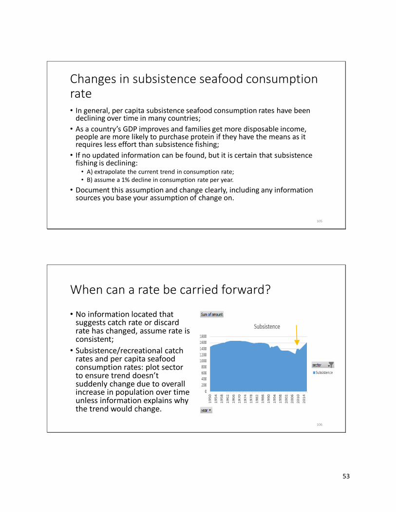
• No information located that suggests catch rate or discard rate has changed, assume rate is consistent;
• Subsistence/recreational catch rates and per capita seafood consumption rates: plot sector to ensure trend doesn’t suddenly change due to overall increase in population over time unless information explains why the trend would change.
106

54
Population data revised
0
1000000
2000000
3000000
4000000
5000000
6000000
7000000
8000000
9000000
10000000
1950
1953
1956
1959
1962
1965
1968
1971
1974
1977
1980
1983
1986
1989
1992
1995
1998
2001
2004
2007
2010
2013
2016
Population revised
previous population data new population data
0
1000000
2000000
3000000
4000000
5000000
6000000
7000000
8000000
9000000
10000000
1950
1953
1956
1959
1962
1965
1968
1971
1974
1977
1980
1983
1986
1989
1992
1995
1998
2001
2004
2007
2010
2013
2016
Population
• Check population trend to make sure no unexplained sudden rise in catch due to revised population data;• Make retroactive changes to catch data at point where versions of population data diverge.
107
National data is no longer available
• Compare national with FAO data:• If FAO data are similar to previous national data, use FAO totals for years to be
updated:• Maintain the reported taxonomic breakdown from the last year of national data; or• If species seem to align, use FAO taxonomic information and match to national taxa.
• If FAO > national data for overlapping years:• Apply adjustment factors to total FAO data so totals match national data amounts.
108

55
Cannot locate any updated information for sector• Some options are:
• Maintain the ratio of unreported to reported catch. Only if catch is not increasing by much (e.g., reporting is not increasing and causing the increase in catch), catch is constant or is in decline;
• If reported catch is increasing, maintain unreported landings at the same tonnage amount (i.e., do not apply the rate) as the last year with data. This will cause a smaller and smaller proportion of catch to be unreported as catch increases while avoiding spikes when catch reporting systems could be increasing;
• Maintain the catch at the amount of the last reconstructed year with data. This is known as flat-lining catch and is the last resort. Note this method is commonly used by FAO for countries that do not report in some years.
• Use the taxonomic and gear breakdowns from the last year with catch.
109
More tools and information
110

56
What other tools are available at seaaroundus.org ?• Some examples are:
• Mapped catch;• End use of catch;• CMSY stock assessments for species that
make up 90% of species identified catch from a marine ecoregion;
• Mariculture database;• Marine Trophic Index;• Stock Status Plots;• Sea bird database;• Estuaries database;• Fisheries subsidies database;• Multinational footprint;• CORU use our catch data with their
parameters for their climate models;• FERU use our data in partnership with
theirs for economic models.
• Soon to be added:• Mean temperature of the catch;• Fishing effort;• Bait;• Transects of catch EEZs.
111
Where to find more information
• Please see the following link on our website: http://www.seaaroundus.org/sea-around-us-methods-index/
• We welcome feedback, and appreciate being informed if factual data errors are detected and communicated to us directly, ideally with:
• The relevant data and information sources that allow correction of such factual errors during the next round of data updates;
• An offer to work with us to correct these errors.
112

57
Acknowledgements… • All Sea Around Us and Sea Around Us – Indian Ocean research is supported by the Minderoo Foundation, the Oak Foundation, the
Marisla Foundation, the Paul M. Angell Family Foundation, the David and Lucile Packard Foundation, Oceana, Bloomberg Philanthropic through RARE, and the MAVA Foundation. Thank you also to previous funding sources: FAO, US Western Pacific Fisheries Management Council, EU-Parliament, UNEP, BOBLME, Rockefeller Foundation.
• Thanks to all members of the Sea Around Us, past and present… visit us at www.seaaroundus.org
And to our research collaborators
113

58
APPENDIX I: TOWARD RANKING MARITIME COUNTRIES BY THE FISH BIOMASS LEFT IN THEIR EEZS2 Abstract The approaches are presented that the Sea Around Us plans to use to rank countries by the biomass of major exploited species that is left in their Exclusive Economic Zones (EEZs), relative to unexploited biomass of each of these species. These approaches are structured around the use of several data-limited stock assessment methods, notably the previously reviewed, tested and published CMSY, BSM and LBB methods. This suite of methods will be applied to fisheries catches reconstructed for the 1950-2016 period, and complemented by stock assessments performed previously by others. The results of most of these ‘other’ assessments can be used either in lieu of our data-limited method assessment results or as informative priors for our assessments. The case is made that countries should be ranked only by their ‘biomass left’, with other (process) variables used for interpretation of the resulting ranking.
Introduction With the development, peer-reviewed testing and increasing availability of the suite of data-limited stock assessment methods developed by the Sea Around Us research partner, Rainer Froese and colleagues (i.e., CMSY and BSM: Froese et al. 2017; LBB: Froese et al. 2018)3 it has become relatively easy to perform stock assessments (i.e., deriving biomass time series of exploited fish4 populations) for any species for which a reasonably long time series of catch, length frequency (L/F) and/or catch per unit effort (CPUE) data are available (e.g., Froese et al. 2018b; Palomares et al. 2018, 2019).
So far, most of these data-limited assessments have been performed for previously defined stocks5 (Froese et al. 2018b) or for species-specific data at the scale of Marine Ecoregions (ME; Spalding et al. 2007), whose CMSY assessments were summarized in Palomares et al. (2018, 2019). The latter is made possible by the unique spatial allocation of fisheries catch data to half degree latitude/longitude cells by the Sea Around Us (Zeller et al. 2016; Palomares et al. 2016), which are then regrouped to conform to any desired geographical entities, e.g. the Exclusive Economic Zones of countries (EEZs), or Large Marine Ecosystems (LME) or the already mentioned MEs (see
2 Drafted by Daniel Pauly, Dirk Zeller, Jessica Meeuwig, Rainer Froese and M.L. ‘Deng’ Palomares in April 2019, for the Minderoo Foundation/Sea Around Us workshop held on 13th – 14th May 2019, in Perth, Western Australia. 3 Another method, AMSY, focused on assessment based mainly on catch/effort (i.e., CPUE) time series is in the final stage of testing and may also be used where appropriate. 4 Here ‘fish’ include teleosts, elasmobranchs and marine invertebrates. 5 ‘Stock’ is here defined as the exploited part of a fish population. Outside of Europe, North America, Australia and New Zealand, exploited ‘stocks’ are generally not well defined (but see Mendo 2018). Thus the use of Marine Ecoregions (ME) to assemble catch date that pertains to geographically and ecologically well-defined entities as a proxy for ‘stock’ areas.

59
www.seaaroundus.org). No other global dataset on marine fisheries has this level of spatial detail or geographical flexibility.
Thus, for large countries or other entities with large EEZs, it is straightforward to estimate how much fish is left in their EEZs, relative to the unexploited state, given that their EEZs will comprise either one complete ME or, more commonly several MEs whose major stocks will have been assessed. For example, the Australian EEZ contains 17 MEs (www.seaaroundus.org/data/#/meow), each with their own sets of assessments. The situation is different for countries with smaller EEZs, and whose marine fisheries are bound to mainly or exclusively exploit stocks shared with neighboring countries. This contribution provides tentative solutions to this quandary and to related issues, i.e., regarding the temporal baseline of the assessments, and their use to derive a single indicator of the biomass left in the waters of each maritime country.
The ‘biomass left’ concept Numerous indicators of fisheries management success have been proposed, and several of them are being used in various countries. However, many of these indicators unhelpfully quantify the management process, or the management effort, but few address what should be the key variable driving management outcomes, i.e., how much fish is left or remains in the sea relative to what was originally there. The classic example of this overemphasis on process is assessments by the Marine Stewardship Council, which is increasingly criticized because of this (Gulbrandsen 2009; Kalfagianni and Pattberg 2013; Hadjimichael and Hegland 2016).
Based on the United Nations Convention on the Law of the Sea (UNCLOS), we take the position that the biomass that should be left in the ocean is that which will generate Maximum Sustainable Yield (shorthand: BMSY), which itself is half the unexploited biomass (Bo, or carrying capacity). Thus, the fraction of current biomass (B) left, for any stock is, according to Schaefer (1954, 1957), B/Bo, or B/(2*BMSY)6.
We view the concept of ‘biomass left’ with reference to the unexploited biomass as inherently easier to convey to the public than biomass-at-MSY (B/BMSY), or even F/FMSY, namely the current fishing mortality with reference to fishing mortality at MSY, which is often used to express the results of stock assessments, but which can be understood only by stock assessment and fisheries management specialists.
The CMSY and other stock assessment methods
The principle of the CMSY method is that multiple biomass trajectories of the biomass of the stock in question are traced using a Monte Carlo approach, and only those the parameters are retained that generate the biomass trajectory (or trajectories) that is (are) compatible with the time series of catches, and a number of constraints (Froese et al. 2017). Here, ‘compatible’ means that, among other things, the stock does not crash, i.e., its biomass drops to zero.
The CSMY method is based on the logic of the surplus-production model of Schaefer (1954, 1957), and thus, it assumes that from one year (t) to the next (t+1), the biomass (Bt) follows the equation:
6 These are some models (notably LBB) which assume that B0 is slightly higher than 2·BMSY; this will be consider on a case-by-case basis.
60
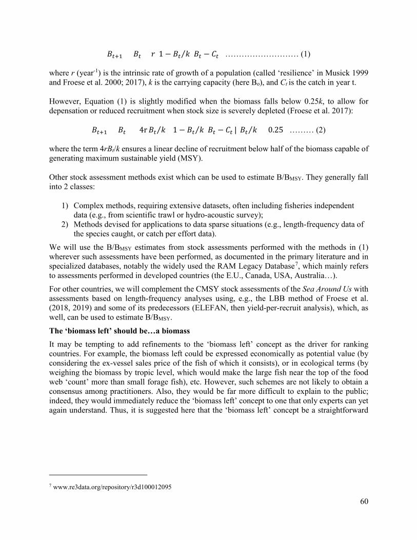
𝐵𝐵𝑡𝑡+1 = 𝐵𝐵𝑡𝑡 + 𝑟𝑟(1 − 𝐵𝐵𝑡𝑡 𝑘𝑘⁄ )𝐵𝐵𝑡𝑡 − 𝐶𝐶𝑡𝑡 ……………………… (1)
where r (year-1) is the intrinsic rate of growth of a population (called ‘resilience’ in Musick 1999 and Froese et al. 2000; 2017), k is the carrying capacity (here Bo), and Ct is the catch in year t.
However, Equation (1) is slightly modified when the biomass falls below 0.25k, to allow for depensation or reduced recruitment when stock size is severely depleted (Froese et al. 2017):
𝐵𝐵𝑡𝑡+1 = 𝐵𝐵𝑡𝑡 + (4r𝐵𝐵𝑡𝑡 𝑘𝑘⁄ )(1− 𝐵𝐵𝑡𝑡 𝑘𝑘⁄ )𝐵𝐵𝑡𝑡 − 𝐶𝐶𝑡𝑡 | 𝐵𝐵𝑡𝑡 𝑘𝑘 < 0.25⁄ ……… (2)
where the term 4rBt/k ensures a linear decline of recruitment below half of the biomass capable of generating maximum sustainable yield (MSY).
Other stock assessment methods exist which can be used to estimate B/BMSY. They generally fall into 2 classes:
1) Complex methods, requiring extensive datasets, often including fisheries independent data (e.g., from scientific trawl or hydro-acoustic survey);
2) Methods devised for applications to data sparse situations (e.g., length-frequency data of the species caught, or catch per effort data).
We will use the B/BMSY estimates from stock assessments performed with the methods in (1) wherever such assessments have been performed, as documented in the primary literature and in specialized databases, notably the widely used the RAM Legacy Database7, which mainly refers to assessments performed in developed countries (the E.U., Canada, USA, Australia…).
For other countries, we will complement the CMSY stock assessments of the Sea Around Us with assessments based on length-frequency analyses using, e.g., the LBB method of Froese et al. (2018, 2019) and some of its predecessors (ELEFAN, then yield-per-recruit analysis), which, as well, can be used to estimate B/BMSY.
The ‘biomass left’ should be…a biomass It may be tempting to add refinements to the ‘biomass left’ concept as the driver for ranking countries. For example, the biomass left could be expressed economically as potential value (by considering the ex-vessel sales price of the fish of which it consists), or in ecological terms (by weighing the biomass by tropic level, which would make the large fish near the top of the food web ‘count’ more than small forage fish), etc. However, such schemes are not likely to obtain a consensus among practitioners. Also, they would be far more difficult to explain to the public; indeed, they would immediately reduce the ‘biomass left’ concept to one that only experts can yet again understand. Thus, it is suggested here that the ‘biomass left’ concept be a straightforward
7 www.re3data.org/repository/r3d100012095

61
expression of the biomass of all (exploitable) fish, relative to the estimated carrying capacity of the ecosystems in which they occur8.
The ‘biomass left’ in countries with stock assessments There are a few, mostly large countries or other entities with large EEZs, encompassing several MEs that independently assess a large fraction of the fish stocks exploited in their waters using a variety of stock assessment methods, all generally deriving B/BMSY estimates. Prominent among them are Australia, the EU, Canada, and the USA.
For these countries, it is proposed that we compare the results of independent assessments (as published in the scientific literature, government literature and/or in the RAM Legacy Stock Assessment Database) with our stock assessments performed using the data-limited suite of methods. This could lead to several outcomes:
i) The ‘other’ assessments, if they are deemed of sufficient quality (e.g., peer-reviewed and well documented) and if they assess the performance of the stock over a sufficient time period, can be used in lieu of our data-limited assessments as the measure of B/BMSY for the given stock that will be used for the GFI. This may also assist in increased buy-in from the stock assessment experts and general scientific community in these countries;
ii) The ‘other’ assessments, if they pertain to species for which our data-limited assessments can be performed, could provide informative ‘priors’ for the data-limited assessments undertaken, which will thus be improved;
iii) When catch data do not exist in the Sea Around Us database for a species with ‘other’ assessment, the estimate of B/BMSY from the ‘other’ assessment for the species in question can be incorporated into the ‘biomass left’ average for the country in question, weighted by (a) the contribution to the total catch of the assessed species, and (b) the length of the assessment period considered.
Also, it is proposed that all ‘other’ assessments considered should be based on data sampled for at least one year in the 21st century. Or, put differently: time series of catch, CPUE or length-frequency data should end in 2000 or later, such as to avoid old assessments to have an undue influence on our results. All assessments (some weighted as suggested above) should pertain to species jointly contributing to at least 80% of the current catches taken in a given EEZ9.
It will be then assumed that the unassessed taxa, jointly contributing less than 20% of the catches in each EEZ, have been reduced as suggested by the resulting mean B/Bo (i.e., B/(2*BMSY) of the assessed stocks accounting for 80%. Thus, we assume that unassessed taxa experience the same biomass trend as the average of assessed taxa.
8 There will be cases in which that carrying capacity has changed, e.g., due to changes in the frequency of El Niño events in Peru. Such cases will have to be identified, and weighted such that they do not massively influence what should be an index reflecting the success of fisheries management. 9 When a country has several EEZ ‘chunks’ (such as Canada’s East, West and Arctic Coasts), it will be necessary to derive a mean B/BMSY of all the chunks, weighted by the contribution of the catches in each chunk to the total catches in all the EEZs of that country.
62
For EU countries, given the stock sharing resulting from the EU Common Fisheries Policy, the mix of species caught in their EEZs will determine which available B/BMSY values (as estimated earlier by ICES, or recently by Froese et al. 2018) will be used to compute their mean B/Bo
10.
For other countries that have little choice but to provide access to their EEZs to foreign fleets11 which then contribute to overfishing the resources therein, the low B/Bo that will be estimated will be an expression of their political and economic weakness, not necessarily of their management performance per se12.
Estimating the biomass left in countries without stock assessments Some countries, e.g., Albania or Gambia have coastlines so short that they cannot be expected to encompass more than a minute fraction of the distribution ranges of the fish stocks exploited in their small EEZs13. As these countries usually do not perform stock assessments, the mean B/BMSY per stock they exploit will be computed, weighted by the contribution of each species to the catch made within their EEZ.
For example, if a country currently features in its catch mainly wide-ranging species with a low B/BMSY, this country will have a lower mean B/Bo than a country which catches mainly species with a higher B/BMSY.
Argument for using the year 1950 as a baseline When dealing with changes, e.g., the changes inflicted by fishing onto the oceans, it is appropriate to study or use data from as long a period as possible, such that even small changes can be perceived.
The Sea Around Us considered 1950 as the best year to start its time series of reconstructed catches because 1950 was:
1) The first year for which FAO began to publish annual statistics of maritime fish landings for every country in the world;
2) The first year of a decade that saw the rebuilding and beginning of the geographic expansion of post WWII industrial fisheries in the world; and
10 The resulting country-specific B/Bo estimates will thus reflect the ‘deals’ agreed between EU countries, some of them having ‘traded’ certain stocks they do not care about against others they value more. 11 For example, West African countries with rich demersal resources, or small island states in the Pacific, with rich tuna resources. 12 This is where governance or other variables not related to stock abundance will be most useful for interpretation: to explain why a country may have a low B/Bo although it may have the best intentions in the world, but has to accept non-sustainable fishing in its EEZ because it is politically weak and/or economically vulnerable. 13 This does not apply to heavily localized, sedentary stocks of, e.g., bivalves exploited by subsistence fisheries; however, their catch is often very small in overall terms and hence will not influence the results, even for very small countries.

63
3) The first year of the last decade in which Europe and some other countries controlled colonies in Africa, the Caribbean, Asia and the Pacific, thus providing a strong contrast between historic periods.
While detailed accounts of fisheries and catch statistics were sometimes hard to locate for the 1950s and the following decades, they were not necessarily less reliable than more recent statistics and accounts. In fact, the increasing tendency to misreport catch and landings, which grew with the imposition of quotas in more recent decades, and the fact that, in recent years, governments spend decreasing amounts of resources on monitoring their fisheries, will tend to compensate for the relative security of detailed data from 50 years ago.
Thus our CMSY assessments, which cover the years 1950 to the near-present, benefit immensely from being anchored in early catch data, which usually lead to better estimates of carrying capacity Bo (see Appendix).
In contrast, even analytically extremely complex stock assessments (see above), if performed with truncated time series data will tend to underestimate MSY levels and carrying capacity in all cases where a strong industrial fishery operated in the period preceding the sampling program producing the data considered by the assessment. Thus, we consider the unfortunately common practice by stock assessment experts of truncating available catch time series to be at times biased and potentially questionable, as described in the Appendix.
One last thing The Sea Around Us can and will be able to provide mean B/BMSY estimates for all maritime countries of the world in timely fashion, i.e., estimates of the biomass that is left in their water (i.e., B/Bo). With these estimates, it will be straightforward for staff of the Minderoo Foundation to rank all countries of the world by what is unquestionably a standardized and fully comparable measure of their success at managing their fisheries based on the core principles agreed upon by the global community via UNCLOS, namely MSY, which is a measure directly related to B/Bo. It will be tempting to link separate or additional indicators of management success and a host of other indicators to B/Bo, e.g., capturing some aspect of the management process.
We think that such additional indicator(s) should be only used to interpret the country ranking based on B/Bo, but should not be used as a variable impacting the ranking itself, as that would automatically generate a composite indicator, which has been shown numerous times to be nearly impossible to easily interpret and understand (see, e.g., Ocean Health Index). Our focus on “biomass left” is analogous to the use of the prevalence of slavery used to rank countries in the Global Slavery Index, with additional dimensions (i.e. inequality) informing the issue of vulnerability (Minderoo Foundation 2018). Whatever the additional variable(s) may be, if they were to be used jointly with B/Bo to generate a composite ranking, the result would not be a ranking by ‘biomass left’ in the oceans.
Please note that we are not suggesting that additional indicators, such as governance would not be helpful. What is suggested is that they would be most helpful in (i) interpreting the B/Bo ranking, and (ii) providing suggested levers for countries to improve their rank. It is our understanding that item (ii) is the ultimate goal and purpose of the GFI.
We are very interested in the success of the GFI, which will depend on its transparency and simplicity. This is the reason why we suggest to define it in a simple and transparently singular

64
manner, namely as ‘biomass left’, and why we should use process and other variables only for interpretive purposes.
References Froese, R., H. Winker, G. Coro, N. Demirel, A.C. Tsikliras, D. Dimarchopoulou, G. Scarcella, M. Quaas and N. Matz-
Lück. 2018. Status and rebuilding of European fisheries. Marine Policy. 93:159-70. Froese, R., N. Demirel,G. Coro, K.M. Kleisner, and H. Winker. 2017. Estimating fisheries reference points from catch
and resilience. Fish and Fisheries 18:506-526. Gulbrandsen, L.H., 2009. The emergence and effectiveness of the Marine Stewardship Council. Marine Policy 33(4):
654-660. Hadjimichael, M., Hegland, T.J., 2016. Really sustainable? Inherent risks of eco-labeling in fisheries. Fisheries
Research 174: 129–135. Kalfagianni, A., Pattberg, P., 2013. Global fisheries governance beyond the State: unraveling the effectiveness of the
Marine Stewardship Council. Journal of Environmental Studies and Science 3:184–193.
Mendo, J. 2018. Electrophoretic studies of Peruvian anchoveta, Engraulis ringens confirm the existence of distinct North/Central and Southern Socks, p. 16-26 In: Pauly D. and V. Ruiz-Leotaud (eds.), Marine and Freshwater Miscellanea. Fisheries Centre Research Reports 26(2). Institute for the Oceans and Fisheries, University of British Columbia.
Minderoo Foundation. 2018. The Global Slavery Index. Perth, 276 p.
Palomares, M.L.D., J. Woroniak, S.-L. Nöel, G. Tsui, B. Derrick and D. Pauly. 2019. Preliminary stock assessments of small pelagic fish in West Africa. A report prepared by the Sea Around Us for the MAVA Foundation, 29 p.
Palomares, M.L.D., R. Froese, B. Derrick, S.-L. Nöel, G. Tsui, J. Woroniak and D. Pauly. 2018. A preliminary global assessment of the status of exploited marine fish and invertebrate populations. A report prepared by the Sea Around Us for OCEANA, 64 p.
Palomares, M.L.D., W.W.L Cheung, W.W.L. Lam, and D. Pauly. 2016. The distribution of exploited marine biodiversity. pp. 46-58 In Pauly D and Zeller D (eds.), Global Atlas of Marine Fisheries: A critical appraisal of catches and ecosystem impacts. Island Press, Washington, D.C.
Schaefer, M.B. 1954. Some aspects of the dynamics of populations important to the management of the commercial marine fisheries. Bulletin of the Inter-American Tropical Tuna Commission 1:27-56.
Schaefer, M.B. 1957. A study of the dynamics of populations of the fishery for yellowfin tuna in the eastern tropical Pacific Ocean. Bulletin of the Inter-American Tropical Tuna Commission 2:227-268.
Spalding, M.D., H.E. Fox,G.R. Allen, N. Davidson, Z.A. Ferdaña, M. Finlayson, B.S. Halpern, M.A. Jorge, A. Lombana, S.A. Lourie, K.D. Martin, E. McManus, J. Molnar, C.A. Recchia and J. Robertson. 2007. Marine Ecoregions of the World: A Bioregionalization of Coastal and Shelf Areas. Bioscience 57:573-583.

65
APPENDIX II: MANAGEMENT IMPLICATIONS OF SHIFTING BASELINES IN FISH STOCK ASSESSMENTS14
Rebecca Schijns,
Sea Around Us, Institute for the Oceans and Fisheries, University of British Columbia, Vancouver, B.C., Canada.
Introduction
Marine resources are subject to overexploitation all across the globe, and we continue to fish harder and catch less and less fish. In this day and age of rapid, anthropogenic change, we can observe the booms and busts of resources within a single generation. At the same time, change can occur over many generations, where each generation considers the initial existing conditions to be the standard ‘healthy’ baseline. Both of these types of overexploitation are dangerous, however the slow decrease in abundance of a species can go undetected and undervalued until it is too late. This is the phenomenon of ‘shifting baselines’ (Pauly 1995), which can have critical implications for the management and conservation of exploited marine resources.
In the current state of the world’s fisheries, nations and international organizations are calling for better management of fish stocks in order to secure this economically, ecologically, and culturally valuable resource for future generations. In 1982, the United Nations Convention on the Law of the Sea (UN National Assembly 1982) established Exclusive Economic Zones, areas which extend 200 nautical miles from the coast, and announced that measures must be taken to conserve marine resources so that they are capable of producing maximum sustainable yield (MSY). Although the concept of MSY provides the framework for which most fisheries management is now built upon, the majority of fished stocks have no MSY estimates available (Martell and Froese 2013). Therefore, there is a strong need to utilize new methods which open the doors to conduct stock assessments on as many exploited stocks as possible in order to gain a wider understanding of the status of global fisheries and how to move forward with management decisions.
A fisheries stock assessment is a tool used to describe the past and current conditions of a fish stock through examination of the effects of fishing and various factors. Stock assessments are integral to fisheries management and can be used to make predictions about how a fish stock may respond to different management scenarios. Stock assessments require catch, abundance, and biological information over a time series in order to analyze the current stock status with respect to sustainable yields. However, the beginning of a time series is often chosen based on the quality of data record keeping, which in many cases is poor or non-existent, even if fishing was taking place. Therefore, assessments may use a truncated time series, where the starting point chosen not account for relevant historical dynamics. Truncation can mask important trends including historical spawning stock biomass maximum, reduction of population abundance variability, and past recoveries (Prefontaine 2009). The results of such assessments can implicate harmful
14 This report is based on a term paper submitted by a MSc student of Daniel Pauly on March 22, 2019, and added here as an appendix as it wonderfully demonstrates the biasing effect of short time series of catch in assessing MSY and carrying capacity.

66
management decisions, such as setting quotas too high and endangering the ability of the stock to replenish its exploited population. For that reason, it is important to address the phenomenon of shifting baselines as it presents itself in stock assessments and compare it with more robust time series in order to reveal the true status of marine resources. By using the longest time series possible, past trends are exposed and can be used to inform better management decisions.
Methods Utilizing a new method developed by Martell and Froese (2013, updated in 2017) called
Catch Maximum Sustainable Yield (CMSY) allows reference points to be estimated from catch, resilience, and stock status information on data-limited stocks. This can be especially useful for fisheries managers to make informed decisions concerning the status of a stock, in the absence of the variety of other data requirements used by alternative stock assessments. When compared to MSY estimates from full stock assessments, this method shows comparable results and thus can be seen as a good alternative method in data-poor situations (Martell and Froese 2013). In addition, a Bayesian-Schaefer Model (BSM) complements the CMSY model when a time series of relative biomass is available. CMSY analysis is used in this study on selected stocks within the RAM Legacy Stock Assessment Database (RAMLSAD 2018) that exhibit truncated time series (Prefontaine 2009). These stocks were analyzed twice, first with the truncated catch time series, and then again with the updated and expanded catch baseline. The results are shown in stock status plots revealing time series of catch, biomass, exploitation, and the relative stock size versus relative exploitation. As well, the results of the analysis provide fisheries reference points such as MSY, FMSY, and BMSY, which can be useful for fisheries management.
Results The first stock selected in the RAM Legacy Stock Assessment Database is Atlantic herring,
Clupea harengus, in the North Sea. ICES assessed this stock with the stock identifier HERRNS-IIIa-VIId. Two stock assessments were chosen, the first with a catch time series covering the years 1960-2011 and the second from 1947-2017. Therefore, the first stock assessment is truncated by 13 years. In this case, truncation conceals a historical biomass maximum (Prefontaine 2009). However, this concealment does not seem to have implications for management. As seen in Figure 1, the MSY and BMSY results for management use both fall within a similar range where the truncated time series (Figure 1a) experiences MSY at approximately 652,000 tonnes per year and BMSY of 1,910,000 tonnes, while the expanded baseline (Figure 2a) experiences MSY around 693,000 tonnes per year and BMSY of 1,917,000 tonnes.
Yellowtail flounder, Limanda ferruginea, stock in the Cape Cod/Gulf of Maine region represents the second stock examined by CMSY and BSM analysis. The Northeast Fisheries Science Center (NEFSC) assessed this stock under the identifier YELLCODGOM. The truncated assessment of this stock, shown in Figure 2a, uses the catch time series of 1985-2014, while the expanded baseline, shown in Figure 2b, uses a time series of 1935-2007. In this case, the truncation of 50 years has serious implications for management and conceals historical biomass maximum as well as a steep decline in biomass. As a result, the truncated time series estimates MSY around 1740 tonnes per year and BMSY of 3850 tonnes, while the expanded baseline estimates MSY at 3430 tonnes year and BMSY around 8170 tonnes. Therefore, concealment of historical trends leads to sustainable yield estimates doubling when historical time series are extended. As well, the lower right panels of both Figure 2a and 2b show the estimate of relative biomass (B/BMSY). The truncated stock is perceived to be in the healthy range in recent years while the more robust

67
assessment shows the stock is being overfished. This is due to the narrow scope that the truncated assessment uses to provide a lower estimation of MSY and BMSY, which in turn allows the stock to look healthier than the reality.
The final stock chosen is Atlantic herring, Clupea harengus, in the North Irish Sea, assessed by ICES under the stock identifier HERRNIRS. The time series experiencing a 19-year truncation is shown by the 1980-2017 assessment of the stock (Figure 3a), while the 1961-2015 assessment (Figure 3b) exhibits an expanded baseline. As seen in the upper right panel in Figure 3b, this stock experiences a recovery from low initial biomass, historical biomass maximum, and another depletion before the next truncated time series begins. The truncated assessment estimates MSY at 6500 tonnes per year and BMSY at 21600 tonnes, while the expanded assessment estimates MSY around 12100 tonnes per year and BMSY at 50,000 tonnes. In addition, the lower right panel in Figure 3a and 3b shows the differences between stock status perceptions, as the truncated stock is shown in the healthy range, while the expanded stock presents as overfished. In summation, both fisheries reference points and stock status perceptions are affected by truncation.
Discussion Fishing has been occurring for thousands of years and now, we have reached a critical point
in history where the majority of global fisheries are overexploited and in need of management measures to protect and rebuild stocks before they reach depletion. Unfortunately, fishing is poorly represented in historical records, where oftentimes records and assessments select a starting point that does not represent the full scale of change. This truncation has direct influence on how we view ecosystems in terms of “healthy” and “unhealthy”. Therefore, we must demand a reset of baselines for those that have shifted, and reconstruct historical catches where records are lacking, as we do not have the luxury of time or resource security to continue to accept progressively unhealthy fish stocks (Pauly 1995).
As shown by Prefontaine (2009), truncations appear in many stock assessments by various fisheries management bodies, and this effect conceals patterns of recoveries, low abundance levels, fluctuations, historical spawning stock biomass maxima, and other dynamics. Using the CMSY method to analyze three stocks, which exhibited truncated time series, shows that there are differences between using truncated or extended time series, and this can have implications for fisheries reference points used by management. Stocks that undergo similar patterns of biomass fluctuations in both lengthened and shortened time series, such as the North Sea herring stock, may not be affected by truncation. However, assessed truncated stocks which discount historical biomass declines, such as the Irish North Sea herring stock and yellowtail flounder stock in Cape Cod/Gulf of Maine, can shift the baseline of MSY and produce reference points that are ill-informed and narrow in scope. This ultimately can create a false perception of stock health, from which conservation initiatives and management can build upon, further diluting the misconception that a stock may be ‘healthy’ or ‘unhealthy’.
We have become accustomed to setting our standards lower each generation that we accept the extractive practices conducted in the ocean without taking a second to step back and reassess what a ‘healthy’ ecosystem should look like. Therefore, it is useful and necessary to use extended time series wherever possible in combination with approaches such as the CMSY method to allow for data-poor stocks to be assessed. Through building our understanding on the history of human’s impact on marine ecosystems around the world, we can better comprehend how marine resources respond to fishing pressures and create management frameworks to improve their status.

68
References Froese, R., Demirel, N., Coro, G., Kleisner, K. M., & Winker, H. (2017). Estimating fisheries
reference points from catch and resilience. Fish and Fisheries 18(3):506-526.
Martell, S., & Froese, R. (2013). A simple method for estimating MSY from catch and resilience. Fish and Fisheries 14(4):504-514.
Pauly, D. (1995). Anecdotes and the shifting baseline syndrome of fisheries. Trends in Ecology & Evolution 10(10):430.
Prefontaine, R. (2009). Shifting baselines in marine fish assessments: implications for perception of management and conservation status. Honours Bachelor Thesis, Dalhousie University, Halifax.
RAM Legacy Stock Assessment Database. 2018. Version 4.44-assessment-only. Released 2018-12-22. Accessed [2019-03-15]. Retrieved from DOI:10.5281/zenodo.2542919.
UN General Assembly, Convention on the Law of the Sea, 10 December 1982, available at: http://www.un.org/depts/los/convention_agreements/texts/unclos/closindx.htm [accessed 20 March 2019]

69
Figure 1a. Summary report for truncated time series of Atlantic herring (1960-2011), Clupea harengus, in the North Sea, which presents results for management use. Grey areas indicate 95% confidence limits in the upper panels and lower left graph. The lower right panel shows the trajectory of relative stock size (B/BMSY) as a function of fishing pressure (F/FMSY). The “banana” shape around the assessment of the final year triangle indicates uncertainty with yellow for 50%, grey for 80% and dark grey for 95% confidence levels.

70
Figure 1b: Summary report for Atlantic herring (1947-2017), Clupea harengus, in the North Sea, which presents results for management use. Grey areas indicate 95% confidence limits in the upper panels and lower left graph. The lower right panel shows the trajectory of relative stock size (B/BMSY) as a function of fishing pressure (F/FMSY). The “banana” shape around the assessment of the final year triangle indicates uncertainty with yellow for 50%, grey for 80% and dark grey for 95% confidence levels.

71
Figure 2a: Summary report for truncated time series of Yellowtail flounder (1985-2014), Limanda ferruginea, in Cape Cod/The Gulf of Maine, which presents results for management use. Grey areas indicate 95% confidence limits in the upper panels and lower left graph. The lower right panel shows the trajectory of relative stock size (B/BMSY) as a function of fishing pressure (F/FMSY). The “banana” shape around the assessment of the final year triangle indicates uncertainty with yellow for 50%, grey for 80% and dark grey for 95% confidence levels.

72
Figure 2b: Summary report for Yellowtail flounder (1935-2007), Limanda ferruginea, in Cape Cod/The Gulf of Maine, which presents results for management use. Grey areas indicate 95% confidence limits in the upper panels and lower left graph. The lower right panel shows the trajectory of relative stock size (B/BMSY) as a function of fishing pressure (F/FMSY). The “banana” shape around the assessment of the final year triangle indicates uncertainty with yellow for 50%, grey for 80% and dark grey for 95% confidence levels.

73
Figure 3a: Summary report for truncated time series of Atlantic herring (1980-2017), Clupea harengus, in the North Irish Sea, which presents results for management use. Grey areas indicate 95% confidence limits in the upper panels and lower left graph. The lower right panel shows the trajectory of relative stock size (B/BMSY) as a function of fishing pressure (F/FMSY). The “banana” shape around the assessment of the final year triangle indicates uncertainty with yellow for 50%, grey for 80% and dark grey for 95% confidence levels.

74
Figure 3b: Summary report for Atlantic herring (1960-2015), Clupeid harengus, in the North Irish Sea, which presents results for management use. Grey areas indicate 95% confidence limits in the upper panels and lower left graph. The lower right panel shows the trajectory of relative stock size (B/BMSY) as a function of fishing pressure (F/FMSY). The “banana” shape around the assessment of the final year triangle indicates uncertainty with yellow for 50%, grey for 80% and dark grey for 95% confidence levels.


OTHER TITLES IN THIS SERIES Pauly D (2005) Sea Around Us: A Five-Year Retrospective 1999 to 2004. Sea Around Us project, Fisheries Centre,
University of British Columbia, Vancouver, 56 p.
Pauly D, Booth S, Christensen V, Cheung WL, Close C, Kitchingman A, Palomares MLD, Watson R, Zeller D (2005). On the exploitation of elasmobranchs, with emphasis on cowtail stingray Pastinachus sephen (Family Dasyatidae). A report of the Sea Around Us Project to the Pew Charitable Trusts. University of British Columbia, Vancouver, 37 p.
Pauly D (2010) Sea Around Us: A Ten-Year Retrospective, 1999 to 2009. Sea Around Us project, Fisheries Centre, University of British Columbia, Vancouver, 57 p.
Biery L, Palomares MLD, Morissette L, Cheung WWL, Harper S, Jacquet J, Zeller D and Pauly D (2011) Sharks in the seas around us: How the Sea Around Us Project is working to shape our collective understanding of global shark fisheries. A report prepared for the Pew Environment Group by the Sea Around Us Project. The University of British Columbia, Vancouver, 53 p.
Cheung WWL, Zeller D and Pauly D (2011) Projected species shift due to climate change in the Canadian Marine Ecoregions. A report of the Sea Around Us Project to Environment Canada. University of British Columbia, Vancouver, 46 p.
Palomares MLD, Chaitanya D, Harper S, Zeller D and Pauly D (2011) The marine biodiversity and fisheries catches of the Pitcairn Group. A report prepared for the Global Ocean Legacy project of the Pew Environment Group by the Sea Around Us Project, Fisheries Centre, University of British Columbia, Vancouver, 42 p.
Kleisner K, Coll M, Christensen V, Boonzaier L, McCrea- Strub A, Zeller D, Pauly D (2012) Towards increasing fisheries’ contribution to food security. Part II: The potentials of 25 fishing countries. A report of the Sea Around Us Project to Oceana and the Bloomberg and Rockefeller Foundations. University of British Columbia, Vancouver, 148 p.
Palomares MLD, Harper S, Zeller D and Pauly D, editors (2012) The marine biodiversity and fisheries catches of the Kermadec island group. A report prepared for the Global Ocean Project of the Pew Environment Group by the Sea Around Us Project. University of British Columbia, Vancouver. 47 p.
Pauly D, Kleisner K, Bhathal B, Boonzaier L, Freire K, Greer K, Hornby C, Lam V, Palomares MLD, McCrea- Strub A, van der Meer L, Zeller D (2012) Towards increasing fisheries’ contribution to food security. Part I: The potentials of Brazil, Chile, India and the Philippines. A report of the Sea Around Us Project to Oceana and the Bloomberg and Rockefeller Foundations. University of British Columbia, Vancouver, 109 p
Kleisner K, Pauly D, Zeller D, Palomares MLD, Knip D, Tavakolie A, Boonzaier L and Cisneros Montemayor A (2013) Country performance in living marine resources exploitation and governance: a foundation for decision-making. A report of the Sea Around Us project to The Rockefeller Foundation. Fisheries Centre, University of British Columbia, Vancouver. 91 p.
Pauly D, Zeller D (Editors) (2014) So long, and thanks for all the fish: the Sea Around Us, 1999-2014 – a fifteen-year retrospective. A Sea Around Us Report to The Pew Charitable Trusts, University of British Columbia, Vancouver. 171 p.
Ruiz-Leotaud, V. and D. Pauly. 2018. The fisheries in and around Coiba National Park, Panama. A Sea Around Us report to UNESCO. 44 p. [Distribution restricted].
Palomares MLD, Froese R, Derrick B, Nöel S-L, Tsui G, Woroniak J, Pauly D (2018) A preliminary global assessment of the status of exploited marine fish and invertebrate populations. A report prepared by the Sea Around Us for OCEANA. The University of British Columbia, Vancouver, p. 64.
Palomares MLD, Derrick B, Nöel S-L, Tsui G, Woroniak J, Pauly D (2019) Preliminary stock assessments of small pelagic fish populations off West Africa. A report prepared by the Sea Around Us for the MAVA Foundation. January 23 2019. The University of British Columbia, Vancouver, p. 39.

www.seaaroundus.org
Sea Around UsInstitute for the Oceans and FisheriesUniversity of British Columbia2202 Main Mall, Vancouver BCV6T1Z4 Canada