Embed Size (px)
Citation preview

scVI DocumentationRelease 0.6.4
Romain Lopez
May 22, 2020


CONTENTS
1 Installation 3
2 Tutorials 5
3 Contributed tutorials 115
4 Contributing 137
5 History 141
6 References 145
7 scvi.dataset package 147
8 scvi.inference package 167
9 scvi.models package 199
10 scvi.models.modules package 215
11 Indices and tables 223
Bibliography 225
Python Module Index 227
Index 229
i

ii

scVI Documentation, Release 0.6.4
Key contributors
scVI graph | # = maintainer, = diverse contributions
• Romain Lopez: scVI lead, , #
• Adam Gayoso: totalVI lead, LDVAE, , #
• Pierre Boyeau: differential expression, , #
• Jeffrey Regier: initial scVI package,
• Chenling Xu : scANVI,
• Valentine Svensson: LDVAE,
• Oscar Clivio : AutoZI,
• Achille Nazaret : gimVI, GeneExpressionDataset,
• Gabriel Misrachi : autotune, GeneExpressionDataset,
• Yining Liu : data loading, preprocessing,
• Jules Samaran : gimVI,
• Maxime Langevin : gimVI,
• Edouard Mehlman : code infrastructure, scANVI,
scVI is a package for end-to-end analysis of single-cell omics data. The package is composed of several deep genera-tive models for omics data analysis, namely:
• scVI for analysis of single-cell RNA-seq data [Lopez18]
• scANVI for cell annotation of scRNA-seq data using semi-labeled examples [Xu19]
• totalVI for analysis of CITE-seq data [Gayoso19]
• gimVI for imputation of missing genes in spatial transcriptomics from scRNA-seq data [Lopez19]
• AutoZI for assessing gene-specific levels of zero-inflation in scRNA-seq data [Clivio19]
• LDVAE for an interpretable linear factor model version of scVI [Svensson20]
These models are able to simultaneously perform many downstream tasks such as learning low-dimensional cellrepresentations, harmonizing datasets from different experiments, and identifying differential expressed features[Boyeau19]. By levaraging advances in stochastic optimization, these models scale to millions of cells. We inviteyou to explore these models in our tutorials.
• If you find a model useful for your research, please consider citing the corresponding publication.
CONTENTS 1

scVI Documentation, Release 0.6.4
2 CONTENTS

CHAPTER
ONE
INSTALLATION
1.1 Prerequisites
1. Install Python 3.7. We typically use the Miniconda Python distribution and Linux.
2. Install PyTorch. If you have an Nvidia GPU, be sure to install a version of PyTorch that supports it – scVI runsmuch faster with a discrete GPU.
1.2 scVI installation
Install scVI in one of the following ways:
Through conda:
conda install scvi -c bioconda -c conda-forge
Through pip:
pip install scvi
Through pip with packages to run notebooks. This installs scanpy, etc.:
pip install scvi[notebooks]
Nightly version - clone this repo and run:
pip install .
For development - clone this repo and run:
pip install -e .[test,notebooks]
If you wish to use multiple GPUs for hyperparameter tuning, install MongoDb.
3

scVI Documentation, Release 0.6.4
4 Chapter 1. Installation

CHAPTER
TWO
TUTORIALS
The easiest way to get familiar with scVI is to follow along with our tutorials! The tutorials are accessible on thesidebar to the left. Some are designed to work seamlessly in Google Colab, a free cloud computing platform. Thesetutorials have a Colab badge in their introduction.
To download the tutorials:
1. Click the Colab badge below
2. Open the tutorial
3. Download it with the option in the file menu.
4. When you execute the notebook yourself, please set your own save_path.
Also, please pardon the code at the beginning of tutorials that is used for testing our notebooks. Testing the notebooksis important so we do not introduce any bugs!
2.1 Introduction to single-cell Variational Inference (scVI)
In this introductory tutorial, we go through the different steps of a scVI workflow
1. Loading the data
2. Training the model
3. Retrieving the latent space and imputed values
4. Visualize the latent space with scanpy
5. Perform differential expression
6. Correcting batch effects with scVI
7. Miscenalleous information
[ ]: # If running in Colab, navigate to Runtime -> Change runtime type# and ensure you're using a Python 3 runtime with GPU hardware accelerator# Installation of scVI in Colab can take several minutes
[ ]: import sysIN_COLAB = "google.colab" in sys.modules
(continues on next page)
5

scVI Documentation, Release 0.6.4
(continued from previous page)
def allow_notebook_for_test():print("Testing the basic tutorial notebook")
show_plot = Truetest_mode = Falsesave_path = "data/"
if not test_mode:save_path = "../../data"
if IN_COLAB:!pip install --quiet git+https://github.com/yoseflab/scvi@stable
→˓#egg=scvi[notebooks]
[ ]: import osimport numpy as npimport pandas as pdimport matplotlib.pyplot as pltfrom scvi.dataset import CortexDataset, RetinaDatasetfrom scvi.models import VAEfrom scvi.inference import UnsupervisedTrainer, load_posteriorfrom scvi import set_seedimport torch
# Control UMAP numba warningsimport warnings; warnings.simplefilter('ignore')
if IN_COLAB:%matplotlib inline
# Sets torch and numpy random seeds, run after all scvi importsset_seed(0)
2.1.1 Loading data
Let us first load the CORTEX dataset described in Zeisel et al. (2015). scVI has many “built-in” datasets as well assupport for loading arbitrary .csv, .loom, and .h5ad (AnnData) files. Please see our data loading Jupyter notebook formore examples of data loading.
• Zeisel, Amit, et al. “Cell types in the mouse cortex and hippocampus revealed by single-cell RNA-seq.” Science347.6226 (2015): 1138-1142.
[ ]: gene_dataset = CortexDataset(save_path=save_path, total_genes=None)gene_dataset.subsample_genes(1000, mode="variance")# we make the gene names lower case just for this tutorial# scVI datasets preserve the case of the gene names as they are in the source filesgene_dataset.make_gene_names_lower()
[2020-01-29 07:41:10,549] INFO - scvi.dataset.dataset | File /data/expression.bin→˓already downloaded[2020-01-29 07:41:10,553] INFO - scvi.dataset.cortex | Loading Cortex data[2020-01-29 07:41:19,357] INFO - scvi.dataset.cortex | Finished preprocessing Cortex→˓data[2020-01-29 07:41:19,790] INFO - scvi.dataset.dataset | Remapping labels to [0,N][2020-01-29 07:41:19,792] INFO - scvi.dataset.dataset | Remapping batch_indices to [0,→˓N]
(continues on next page)
6 Chapter 2. Tutorials

scVI Documentation, Release 0.6.4
(continued from previous page)
[2020-01-29 07:41:21,050] INFO - scvi.dataset.dataset | Downsampling from 19972 to→˓1000 genes[2020-01-29 07:41:21,078] INFO - scvi.dataset.dataset | Computing the library size→˓for the new data[2020-01-29 07:41:21,090] INFO - scvi.dataset.dataset | Filtering non-expressing→˓cells.[2020-01-29 07:41:21,101] INFO - scvi.dataset.dataset | Computing the library size→˓for the new data[2020-01-29 07:41:21,106] INFO - scvi.dataset.dataset | Downsampled from 3005 to 3005→˓cells[2020-01-29 07:41:21,107] INFO - scvi.dataset.dataset | Making gene names lower case
[ ]: # Representation of the dataset objectgene_dataset
GeneExpressionDataset object with n_cells x nb_genes = 3005 x 1000gene_attribute_names: 'gene_names'cell_attribute_names: 'local_vars', 'local_means', 'batch_indices', 'precise_
→˓labels', 'labels'cell_categorical_attribute_names: 'labels', 'batch_indices'
In this demonstration and for this particular dataset, we use only 1000 genes as this dataset contains only 3005 cells.Furthermore, we select genes that have high variance across cells. By default, scVI uses an adapted version of theSeurat v3 vst gene selection and we recommend using this default mode.
Here are few practical rules for gene filtering with scVI:
• If many cells are available, it is in general better to use as many genes as possible. Of course, it might be ofinterest to remove ad-hoc genes depending on the downstream analysis or the application.
• When the dataset is small, it is usually better to filter out genes to avoid overfitting. In the original scVIpublication, we reported poor imputation performance for when the number of cells was lower than the numberof genes. This is all empirical and in general, it is hard to predict what the optimal number of genes will be.
• Generally, we advise relying on scanpy (and anndata) to load and preprocess data and then import the unnor-malized filtered count matrix into scVI (see data loading tutorial). This can be done by putting the raw countsin adata.raw, or by using layers.
2.1.2 Training
• n_epochs: Number of epochs (passes through the entire dataset) to train the model. The number of epochsshould be set according to the number of cells in your dataset. For example, 400 epochs is generally fine for< 10,000 cells. 200 epochs or fewer for greater than 10,000 cells. One should monitor the convergence of thetraining/test loss to determine the number of epochs necessary. For very large datasets (> 100,000 cells) youmay only need ~10 epochs.
• lr: learning rate. Set to 0.001 here.
• use_cuda: Set to true to use CUDA (GPU required)
[ ]: n_epochs = 400lr = 1e-3use_cuda = True
We now create the model and the trainer object. We train the model and output model likelihood every 5 epochs. Inorder to evaluate the likelihood on a test set, we split the datasets (the current code can also do train/validation/test,
2.1. Introduction to single-cell Variational Inference (scVI) 7

scVI Documentation, Release 0.6.4
if a test_size is specified and train_size + test_size < 1, then the remaining cells get placed into avalidation_set).
If a pre-trained model already exist in the save_path then load the same model rather than re-training it. This isparticularly useful for large datasets.
train_size: In general, use a train_size of 1.0. We use 0.9 to monitor overfitting (ELBO on held-out data)
[ ]: vae = VAE(gene_dataset.nb_genes)trainer = UnsupervisedTrainer(
vae,gene_dataset,train_size=0.90,use_cuda=use_cuda,frequency=5,
)
[ ]: trainer.train(n_epochs=n_epochs, lr=lr)
training: 100%|| 400/400 [01:53<00:00, 3.51it/s]
Plotting the likelihood change across the 500 epochs of training: blue for training error and orange for testingerror.
[ ]: elbo_train_set = trainer.history["elbo_train_set"]elbo_test_set = trainer.history["elbo_test_set"]x = np.linspace(0, 400, (len(elbo_train_set)))plt.plot(x, elbo_train_set, label="train")plt.plot(x, elbo_test_set, label="test")plt.ylim(1500, 3000)plt.legend()
<matplotlib.legend.Legend at 0x7fa4f35a3b00>
8 Chapter 2. Tutorials

scVI Documentation, Release 0.6.4
2.1.3 Obtaining the posterior object and sample latent space as well as imputationfrom it
The posterior object contains a model and a gene_dataset, as well as additional arguments that for Pytorch’sDataLoader. It also comes with many methods or utilities querying the model, such as differential expression,imputation and differential analyisis.
To get an ordered output result, we use the .sequential() posterior method, which returns another instance ofposterior (with shallow copy of all its object references), but where the iteration is in the same ordered as its indicesattribute.
[ ]: full = trainer.create_posterior(trainer.model, gene_dataset, indices=np.→˓arange(len(gene_dataset)))# Updating the "minibatch" size after training is useful in low memory configurationsfull = full.update({"batch_size":32})latent, batch_indices, labels = full.sequential().get_latent()batch_indices = batch_indices.ravel()
Similarly, it is possible to query the imputed values via the imputation method of the posterior object.
Imputation is an ambiguous term and there are two ways to perform imputation in scVI. The first way is to querythe mean of the negative binomial distribution modeling the counts. This is referred to as sample_rate in thecodebase and can be reached via the imputationmethod. The second is to query the normalized mean of the samenegative binomial (please refer to the scVI manuscript). This is referred to as sample_scale in the codebase andcan be reached via the get_sample_scale method. In differential expression for example, we of course rely onthe normalized latent variable which is corrected for variations in sequencing depth.
[ ]: imputed_values = full.sequential().imputation()normalized_values = full.sequential().get_sample_scale()
The posterior object provides an easy way to save an experiment that includes not only the trained model, but also theassociated data with the save_posterior and load_posterior tools.
Saving and loading results
[ ]: # saving step (after training!)save_dir = os.path.join(save_path, "full_posterior")if not os.path.exists(save_dir):
full.save_posterior(save_dir)
[ ]: # loading step (in a new session)retrieved_model = VAE(gene_dataset.nb_genes) # uninitialized modelsave_dir = os.path.join(save_path, "full_posterior")
retrieved_full = load_posterior(dir_path=save_dir,model=retrieved_model,use_cuda=use_cuda,
)
2.1. Introduction to single-cell Variational Inference (scVI) 9

scVI Documentation, Release 0.6.4
2.1.4 Visualizing the latent space with scanpy
scanpy is a handy and powerful python library for visualization and downstream analysis of single-cell RNA sequenc-ing data. We show here how to feed the latent space of scVI into a scanpy object and visualize it using UMAP asimplemented in scanpy. More on how scVI can be used with scanpy on this notebook. Note to advanced users: Thecode get_latent() returns only the mean of the posterior distribution for the latent space. However, we recover afull distribution with our inference framework. Let us keep in mind that the latent space visualized here is a practicalsummary of the data only. Uncertainty is needed for other downstream analyses such as differential expression.
[ ]: import scanpy as scimport anndata
[ ]: post_adata = anndata.AnnData(X=gene_dataset.X)post_adata.obsm["X_scVI"] = latentpost_adata.obs['cell_type'] = np.array([gene_dataset.cell_types[gene_dataset.→˓labels[i][0]]
for i in range(post_adata.n_obs)])sc.pp.neighbors(post_adata, use_rep="X_scVI", n_neighbors=15)sc.tl.umap(post_adata, min_dist=0.3)
[ ]: fig, ax = plt.subplots(figsize=(7, 6))sc.pl.umap(post_adata, color=["cell_type"], ax=ax, show=show_plot)
... storing 'cell_type' as categorical
The user will note that we imported curated labels from the original publication. Our interface with scanpy makes iteasy to cluster the data with scanpy from scVI’s latent space and then reinject them into scVI (e.g., for differentialexpression). We discuss this in the scanpy tutorial.
10 Chapter 2. Tutorials

scVI Documentation, Release 0.6.4
2.1.5 Differential Expression
From the trained VAE model we can sample the gene expression rate for each gene in each cell. For the two populationsof interest, we can then randomly sample pairs of cells, one from each population to compare their expression ratefor a gene. The degree of differential expression is measured by logit 𝑝
(1−𝑝) where p is the probability of a cell frompopulation A having a higher expression than a cell from population B. We can form the null distribution of the DEvalues by sampling pairs randomly from the combined population.
The following example is implemented for the cortext dataset, vary cell_types and genes_of_interest for otherdatasets.
1. Set population A and population B for comparison
[ ]: cell_types = gene_dataset.cell_typesprint(gene_dataset.cell_types)# oligodendrocytes (#4) VS pyramidal CA1 (#5)couple_celltypes = (4, 5) # the couple types on which to study DE
print("\nDifferential Expression A/B for cell types\nA: %s\nB: %s\n" %tuple((cell_types[couple_celltypes[i]] for i in [0, 1])))
cell_idx1 = gene_dataset.labels.ravel() == couple_celltypes[0]cell_idx2 = gene_dataset.labels.ravel() == couple_celltypes[1]
['astrocytes_ependymal' 'endothelial-mural' 'interneurons' 'microglia''oligodendrocytes' 'pyramidal CA1' 'pyramidal SS']
Differential Expression A/B for cell typesA: oligodendrocytesB: pyramidal CA1
2. Define parameters * n_samples: the number of times to sample px_scales from the vae model for each gene ineach cell. * M_permutation: Number of pairs sampled from the px_scales values for comparison.
[ ]: n_samples = 100M_permutation = 100000
[ ]: de_res = full.differential_expression_score(cell_idx1,cell_idx2,n_samples=n_samples,M_permutation=M_permutation,
)
3. Print out the differential expression value * bayes_factor: The bayes factor for cell type 1 having a higherexpression than cell type 2 * proba_m1: The numerator of the bayes_factor quotient, the probability cell type 1has higher expression than cell type 2 * proba_m2: The denominator of the bayes_factor quotient, equal to 1 minusproba_m1 * raw_meani: average UMI counts in cell type i * non_zeros_proportioni: proportion of non-zero expressionin cell type i * raw_normalized_meani: average UMI counts in cell type i normalized by cell size * scalei: averagescVI imputed gene expression scale in cell type i
[ ]: genes_of_interest = ["thy1", "mbp"]de_res.filter(items=genes_of_interest, axis=0)
proba_m1 proba_m2 ... raw_normalized_mean1 raw_normalized_mean2thy1 0.01084 0.98916 ... 0.089729 1.444312mbp 0.99060 0.00940 ... 8.840034 0.298456
(continues on next page)
2.1. Introduction to single-cell Variational Inference (scVI) 11

scVI Documentation, Release 0.6.4
(continued from previous page)
[2 rows x 11 columns]
9. Visualize top 10 most expressed genes per cell types
[ ]: per_cluster_de, cluster_id = full.one_vs_all_degenes(cell_labels=gene_dataset.labels.→˓ravel(), min_cells=1)
markers = []for x in per_cluster_de:
markers.append(x[:10])markers = pd.concat(markers)
genes = np.asarray(markers.index)expression = [x.filter(items=genes, axis=0)['raw_normalized_mean1'] for x in per_→˓cluster_de]expression = pd.concat(expression, axis=1)expression = np.log10(1 + expression)expression.columns = gene_dataset.cell_types
HBox(children=(FloatProgress(value=0.0, max=7.0), HTML(value='')))
[ ]: plt.figure(figsize=(20, 20))im = plt.imshow(expression, cmap='viridis', interpolation='none', aspect='equal')ax = plt.gca()ax.set_xticks(np.arange(0, 7, 1))ax.set_xticklabels(gene_dataset.cell_types, rotation='vertical')ax.set_yticklabels(genes)ax.set_yticks(np.arange(0, 70, 1))ax.tick_params(labelsize=14)plt.colorbar(shrink=0.2)
<matplotlib.colorbar.Colorbar at 0x7fa49b3e3f28>
12 Chapter 2. Tutorials

scVI Documentation, Release 0.6.4
2.1. Introduction to single-cell Variational Inference (scVI) 13

scVI Documentation, Release 0.6.4
2.1.6 Correction for batch effects
We now load the RETINA dataset that is described in Shekhar et al. (2016) for an example of batch-effect correction.For more extensive utilization, we encourage the users to visit the harmonization as well as the annotation notebookwhich explain in depth how to deal with several datasets (in an unsupervised or semi-supervised fashion).
• Shekhar, Karthik, et al. “Comprehensive classification of retinal bipolar neurons by single-cell transcriptomics.”Cell 166.5 (2016): 1308-1323.
[ ]: retina_dataset = RetinaDataset(save_path=save_path)
[2020-01-29 07:43:41,162] INFO - scvi.dataset.dataset | File /data/retina.loom→˓already downloaded[2020-01-29 07:43:41,163] INFO - scvi.dataset.loom | Preprocessing dataset[2020-01-29 07:43:49,676] INFO - scvi.dataset.loom | Finished preprocessing dataset[2020-01-29 07:43:51,455] INFO - scvi.dataset.dataset | Remapping labels to [0,N][2020-01-29 07:43:51,461] INFO - scvi.dataset.dataset | Remapping batch_indices to [0,→˓N]
[ ]: retina_dataset
GeneExpressionDataset object with n_cells x nb_genes = 19829 x 13166gene_attribute_names: 'gene_names'cell_attribute_names: 'labels', 'batch_indices', 'local_vars', 'local_means'cell_categorical_attribute_names: 'labels', 'batch_indices'
[ ]: # Notice that the dataset has two batchesretina_dataset.batch_indices.ravel()[:10]
array([0, 0, 0, 0, 1, 0, 1, 1, 0, 0], dtype=uint16)
[ ]: # Filter so that there are genes with at least 1 umi count in each batch separatelyretina_dataset.filter_genes_by_count(per_batch=True)# Run highly variable gene selectionretina_dataset.subsample_genes(4000)
[2020-01-29 07:43:51,834] INFO - scvi.dataset.dataset | Downsampling from 13166 to→˓13085 genes[2020-01-29 07:43:52,732] INFO - scvi.dataset.dataset | Computing the library size→˓for the new data[2020-01-29 07:43:53,618] INFO - scvi.dataset.dataset | Filtering non-expressing→˓cells.[2020-01-29 07:43:54,345] INFO - scvi.dataset.dataset | Computing the library size→˓for the new data[2020-01-29 07:43:54,677] INFO - scvi.dataset.dataset | Downsampled from 19829 to→˓19829 cells[2020-01-29 07:43:54,681] INFO - scvi.dataset.dataset | extracting highly variable→˓genes
Transforming to str index.
[2020-01-29 07:44:10,054] INFO - scvi.dataset.dataset | Downsampling from 13085 to→˓4000 genes[2020-01-29 07:44:11,878] INFO - scvi.dataset.dataset | Computing the library size→˓for the new data[2020-01-29 07:44:13,050] INFO - scvi.dataset.dataset | Filtering non-expressing→˓cells.[2020-01-29 07:44:14,119] INFO - scvi.dataset.dataset | Computing the library size→˓for the new data[2020-01-29 07:44:14,255] INFO - scvi.dataset.dataset | Downsampled from 19829 to→˓19829 cells (continues on next page)
14 Chapter 2. Tutorials

scVI Documentation, Release 0.6.4
(continued from previous page)
[ ]: n_epochs = 200lr = 1e-3use_batches = Trueuse_cuda = True
# Train the model and output model likelihood every 10 epochs# if n_batch = 0 then batch correction is not performed# this is controlled by the use_batches boolean variablevae = VAE(retina_dataset.nb_genes, n_batch=retina_dataset.n_batches * use_batches)trainer = UnsupervisedTrainer(
vae,retina_dataset,train_size=0.9 if not test_mode else 0.5,use_cuda=use_cuda,frequency=10,
)trainer.train(n_epochs=n_epochs, lr=lr)
[2020-01-29 07:44:15,101] INFO - scvi.inference.inference | KL warmup phase exceeds→˓overall training phaseIf your applications rely on the posterior quality, consider→˓training for more epochs or reducing the kl warmup.training: 100%|| 200/200 [06:21<00:00, 1.91s/it][2020-01-29 07:50:36,512] INFO - scvi.inference.inference | Training is still in→˓warming up phase. If your applications rely on the posterior quality, consider→˓training for more epochs or reducing the kl warmup.
[ ]: # Plotting the likelihood change across the 400 epochs of training:# blue for training error and orange for testing error.
elbo_train = trainer.history["elbo_train_set"]elbo_test = trainer.history["elbo_test_set"]x = np.linspace(0, 200, (len(elbo_train)))plt.plot(x, elbo_train, label="train")plt.plot(x, elbo_test, label="test")plt.ylim(min(elbo_train)-50, 1000)plt.legend()
<matplotlib.legend.Legend at 0x7fa49ba344a8>
2.1. Introduction to single-cell Variational Inference (scVI) 15

scVI Documentation, Release 0.6.4
Computing batch mixing
This is a quantitative measure of how well cells mix in the latent space, and is precisely the information entropy of thebatch annotations of cells in a given cell’s neighborhood, averaged over the dataset.
[ ]: full = trainer.create_posterior(trainer.model, retina_dataset, indices=np.→˓arange(len(retina_dataset)))print("Entropy of batch mixing :", full.entropy_batch_mixing())
Entropy of batch mixing : 0.6212606968643457
Visualizing the mixing
[ ]: full = trainer.create_posterior(trainer.model, retina_dataset, indices=np.→˓arange(len(retina_dataset)))latent, batch_indices, labels = full.sequential().get_latent()
[ ]: post_adata = anndata.AnnData(X=retina_dataset.X)post_adata.obsm["X_scVI"] = latentpost_adata.obs['cell_type'] = np.array([retina_dataset.cell_types[retina_dataset.→˓labels[i][0]]
for i in range(post_adata.n_obs)])post_adata.obs['batch'] = np.array([str(retina_dataset.batch_indices[i][0])
for i in range(post_adata.n_obs)])sc.pp.neighbors(post_adata, use_rep="X_scVI", n_neighbors=15)sc.tl.umap(post_adata)
[ ]: fig, ax = plt.subplots(figsize=(7, 6))sc.pl.umap(post_adata, color=["cell_type"], ax=ax, show=show_plot)fig, ax = plt.subplots(figsize=(7, 6))sc.pl.umap(post_adata, color=["batch"], ax=ax, show=show_plot)
... storing 'cell_type' as categorical
... storing 'batch' as categorical
16 Chapter 2. Tutorials

scVI Documentation, Release 0.6.4
2.1. Introduction to single-cell Variational Inference (scVI) 17

scVI Documentation, Release 0.6.4
2.1.7 Logging information
Verbosity varies in the following way: * logger.setLevel(logging.WARNING) will show a progress bar. *logger.setLevel(logging.INFO) will show global logs including the number of jobs done. * logger.setLevel(logging.DEBUG) will show detailed logs for each training (e.g the parameters tested).
This function’s behaviour can be customized, please refer to its documentation for information about the differentparameters available.
In general, you can use scvi.set_verbosity(level) to set the verbosity of the scvi package. Note that levelcorresponds to the logging levels of the standard python loggingmodule. By default, that level is set to INFO (=20).As a reminder the logging levels are:
Level
Numeric value
CRITICAL
50
ERROR
40
WARNING
30
INFO
20
DEBUG
10
NOTSET
0
[ ]:
2.2 Data Loading Tutorial
[1]: # Below is code that helps us test the notebooks# when not testing, we make the save_path a directory called data# in the scVI root directory, feel free to move anywhere
[2]: def allow_notebook_for_test():print("Testing the data loading notebook")
test_mode = Falsesave_path = "data/"
# Feel free to move this to any convenient locationif not test_mode:
save_path = "../../data"
18 Chapter 2. Tutorials
scVI Documentation, Release 0.6.4
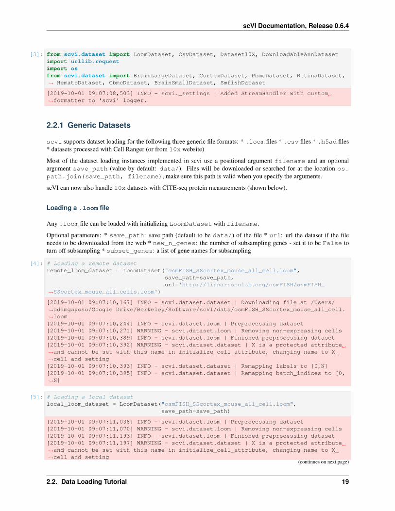
[3]: from scvi.dataset import LoomDataset, CsvDataset, Dataset10X, DownloadableAnnDatasetimport urllib.requestimport osfrom scvi.dataset import BrainLargeDataset, CortexDataset, PbmcDataset, RetinaDataset,→˓ HematoDataset, CbmcDataset, BrainSmallDataset, SmfishDataset
[2019-10-01 09:07:08,503] INFO - scvi._settings | Added StreamHandler with custom→˓formatter to 'scvi' logger.
2.2.1 Generic Datasets
scvi supports dataset loading for the following three generic file formats: * .loom files * .csv files * .h5ad files* datasets processed with Cell Ranger (or from 10x website)
Most of the dataset loading instances implemented in scvi use a positional argument filename and an optionalargument save_path (value by default: data/). Files will be downloaded or searched for at the location os.path.join(save_path, filename), make sure this path is valid when you specify the arguments.
scVI can now also handle 10x datasets with CITE-seq protein measurements (shown below).
Loading a .loom file
Any .loom file can be loaded with initializing LoomDataset with filename.
Optional parameters: * save_path: save path (default to be data/) of the file * url: url the dataset if the fileneeds to be downloaded from the web * new_n_genes: the number of subsampling genes - set it to be False toturn off subsampling * subset_genes: a list of gene names for subsampling
[4]: # Loading a remote datasetremote_loom_dataset = LoomDataset("osmFISH_SScortex_mouse_all_cell.loom",
save_path=save_path,url='http://linnarssonlab.org/osmFISH/osmFISH_
→˓SScortex_mouse_all_cells.loom')
[2019-10-01 09:07:10,167] INFO - scvi.dataset.dataset | Downloading file at /Users/→˓adamgayoso/Google Drive/Berkeley/Software/scVI/data/osmFISH_SScortex_mouse_all_cell.→˓loom[2019-10-01 09:07:10,244] INFO - scvi.dataset.loom | Preprocessing dataset[2019-10-01 09:07:10,271] WARNING - scvi.dataset.loom | Removing non-expressing cells[2019-10-01 09:07:10,389] INFO - scvi.dataset.loom | Finished preprocessing dataset[2019-10-01 09:07:10,392] WARNING - scvi.dataset.dataset | X is a protected attribute→˓and cannot be set with this name in initialize_cell_attribute, changing name to X_→˓cell and setting[2019-10-01 09:07:10,393] INFO - scvi.dataset.dataset | Remapping labels to [0,N][2019-10-01 09:07:10,395] INFO - scvi.dataset.dataset | Remapping batch_indices to [0,→˓N]
[5]: # Loading a local datasetlocal_loom_dataset = LoomDataset("osmFISH_SScortex_mouse_all_cell.loom",
save_path=save_path)
[2019-10-01 09:07:11,038] INFO - scvi.dataset.loom | Preprocessing dataset[2019-10-01 09:07:11,070] WARNING - scvi.dataset.loom | Removing non-expressing cells[2019-10-01 09:07:11,193] INFO - scvi.dataset.loom | Finished preprocessing dataset[2019-10-01 09:07:11,197] WARNING - scvi.dataset.dataset | X is a protected attribute→˓and cannot be set with this name in initialize_cell_attribute, changing name to X_→˓cell and setting
(continues on next page)
2.2. Data Loading Tutorial 19

scVI Documentation, Release 0.6.4
(continued from previous page)
[2019-10-01 09:07:11,198] INFO - scvi.dataset.dataset | Remapping labels to [0,N][2019-10-01 09:07:11,200] INFO - scvi.dataset.dataset | Remapping batch_indices to [0,→˓N]
Loading a .csv file
Any .csv file can be loaded with initializing CsvDataset with filename.
Optional parameters: * save_path: save path (default to be data/) of the file * url: url of the dataset if the fileneeds to be downloaded from the web * compression: set compression as .gz, .bz2, .zip, or .xz to loada zipped csv file * new_n_genes: the number of subsampling genes - set it to be None to turn off subsampling *subset_genes: a list of gene names for subsampling
Note: CsvDataset currently only supoorts .csv files that are genes by cells.
If the dataset has already been downloaded at the location save_path, it will not be downloaded again.
[6]: # Loading a remote datasetremote_csv_dataset = CsvDataset("GSE100866_CBMC_8K_13AB_10X-RNA_umi.csv.gz",
save_path=save_path,new_n_genes=600,compression='gzip',url = "https://www.ncbi.nlm.nih.gov/geo/download/?
→˓acc=GSE100866&format=file&file=GSE100866%5FCBMC%5F8K%5F13AB%5F10X%2DRNA%5Fumi%2Ecsv→˓%2Egz")
[2019-10-01 09:07:39,627] INFO - scvi.dataset.dataset | Downloading file at /Users/→˓adamgayoso/Google Drive/Berkeley/Software/scVI/data/GSE100866_CBMC_8K_13AB_10X-RNA_→˓umi.csv.gz[2019-10-01 09:07:41,457] INFO - scvi.dataset.csv | Preprocessing dataset[2019-10-01 09:09:46,750] INFO - scvi.dataset.csv | Finished preprocessing dataset[2019-10-01 09:09:50,655] INFO - scvi.dataset.dataset | Remapping labels to [0,N][2019-10-01 09:09:50,659] INFO - scvi.dataset.dataset | Remapping batch_indices to [0,→˓N][2019-10-01 09:09:51,992] INFO - scvi.dataset.dataset | Computing the library size→˓for the new data[2019-10-01 09:09:53,389] INFO - scvi.dataset.dataset | Downsampled from 8617 to 8617→˓cells[2019-10-01 09:10:16,073] INFO - scvi.dataset.dataset | Downsampling from 36280 to→˓600 genes[2019-10-01 09:10:16,406] INFO - scvi.dataset.dataset | Computing the library size→˓for the new data[2019-10-01 09:10:16,453] INFO - scvi.dataset.dataset | Filtering non-expressing→˓cells.[2019-10-01 09:10:16,469] INFO - scvi.dataset.dataset | Computing the library size→˓for the new data[2019-10-01 09:10:16,477] INFO - scvi.dataset.dataset | Downsampled from 8617 to 8617→˓cells
[7]: # Loading a local datasetlocal_csv_dataset = CsvDataset("GSE100866_CBMC_8K_13AB_10X-RNA_umi.csv.gz",
save_path=save_path,new_n_genes=600,compression='gzip')
20 Chapter 2. Tutorials
scVI Documentation, Release 0.6.4
[2019-10-01 09:10:16,547] INFO - scvi.dataset.csv | Preprocessing dataset[2019-10-01 09:11:43,587] INFO - scvi.dataset.csv | Finished preprocessing dataset[2019-10-01 09:11:45,660] INFO - scvi.dataset.dataset | Remapping labels to [0,N][2019-10-01 09:11:45,662] INFO - scvi.dataset.dataset | Remapping batch_indices to [0,→˓N][2019-10-01 09:11:46,563] INFO - scvi.dataset.dataset | Computing the library size→˓for the new data[2019-10-01 09:11:47,483] INFO - scvi.dataset.dataset | Downsampled from 8617 to 8617→˓cells[2019-10-01 09:12:05,327] INFO - scvi.dataset.dataset | Downsampling from 36280 to→˓600 genes[2019-10-01 09:12:05,929] INFO - scvi.dataset.dataset | Computing the library size→˓for the new data[2019-10-01 09:12:05,976] INFO - scvi.dataset.dataset | Filtering non-expressing→˓cells.[2019-10-01 09:12:05,995] INFO - scvi.dataset.dataset | Computing the library size→˓for the new data[2019-10-01 09:12:06,005] INFO - scvi.dataset.dataset | Downsampled from 8617 to 8617→˓cells
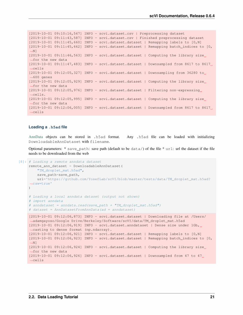
Loading a .h5ad file
AnnData objects can be stored in .h5ad format. Any .h5ad file can be loaded with initializingDownloadableAnnDataset with filename.
Optional parameters: * save_path: save path (default to be data/) of the file * url: url the dataset if the fileneeds to be downloaded from the web
[8]: # Loading a remote anndata datasetremote_ann_dataset = DownloadableAnnDataset(
"TM_droplet_mat.h5ad",save_path=save_path,url='https://github.com/YosefLab/scVI/blob/master/tests/data/TM_droplet_mat.h5ad?
→˓raw=true')
# Loading a local anndata dataset (output not shown)# import anndata# anndataset = anndata.read(save_path + "TM_droplet_mat.h5ad")# dataset = AnnDatasetFromAnnData(ad = anndataset)
[2019-10-01 09:12:06,873] INFO - scvi.dataset.dataset | Downloading file at /Users/→˓adamgayoso/Google Drive/Berkeley/Software/scVI/data/TM_droplet_mat.h5ad[2019-10-01 09:12:06,919] INFO - scvi.dataset.anndataset | Dense size under 1Gb,→˓casting to dense format (np.ndarray).[2019-10-01 09:12:06,921] INFO - scvi.dataset.dataset | Remapping labels to [0,N][2019-10-01 09:12:06,923] INFO - scvi.dataset.dataset | Remapping batch_indices to [0,→˓N][2019-10-01 09:12:06,924] INFO - scvi.dataset.dataset | Computing the library size→˓for the new data[2019-10-01 09:12:06,926] INFO - scvi.dataset.dataset | Downsampled from 47 to 47→˓cells
2.2. Data Loading Tutorial 21

scVI Documentation, Release 0.6.4
Loading outputs from Cell Ranger (10x Genomics)
scVI can download datasets from the 10x website, or load a local directory with outputs generated by Cell Ranger.
10x has published several datasets on their website. Initialize Dataset10X by passing in the dataset name of oneof the following datasets that scvi currently supports. Please check dataset10x.py for a full list of supporteddatasets. If the dataset has already been downloaded at the location save_path, it will not be downloaded again.
The batch indices after the 10x barcode (e.g., AAAAAA-1) is automatically added to the batch_indices datasetattribute.
Optional parameters: * save_path: save path (default to be data/) of the file * type: set type (default to befiltered) to be filtered or raw to choose one from the two datasets that’s available on 10X * dense: bool ofwhether to load as a dense matrix (scVI can be faster since it doesn’t have to densify minibatches). We recommendsetting this to True (not default). * measurement_names_column column in which to find measurement namesin the corresponding .tsv file.
Downloading 10x data
pbmc_10k_protein_v3 is the name of a publicly available dataset from 10x.
[9]: tenX_dataset = Dataset10X("pbmc_10k_protein_v3", save_path=os.path.join(save_path,→˓"10X"), measurement_names_column=1)
[2019-10-01 09:12:06,970] INFO - scvi.dataset.dataset | Downloading file at /Users/→˓adamgayoso/Google Drive/Berkeley/Software/scVI/data/10X/pbmc_10k_protein_v3/→˓filtered_feature_bc_matrix.tar.gz[2019-10-01 09:12:08,414] INFO - scvi.dataset.dataset10X | Preprocessing dataset[2019-10-01 09:12:08,417] INFO - scvi.dataset.dataset10X | Extracting tar file[2019-10-01 09:12:41,192] INFO - scvi.dataset.dataset10X | Finished preprocessing→˓dataset[2019-10-01 09:12:41,346] INFO - scvi.dataset.dataset | Remapping labels to [0,N][2019-10-01 09:12:41,348] INFO - scvi.dataset.dataset | Remapping batch_indices to [0,→˓N][2019-10-01 09:12:41,387] INFO - scvi.dataset.dataset | Computing the library size→˓for the new data[2019-10-01 09:12:41,484] INFO - scvi.dataset.dataset | Downsampled from 7865 to 7865→˓cells
Loading local 10x data
It is also possible to create a Dataset object from 10X data saved locally. Here scVI assumes that in the directorydefined by the save_path there exists another directory with the matrix, features/genes and barcodesfiles. As long as this directory was directly outputted by Cell Ranger and no other files were added, this function willwork. If you are struggling to use this function, you may want to load your data using scanpy and save an AnnDataobject.
In the example below, inside the save path a directory named filtered_feature_bc_matrix exists containingONLY the files barcodes.tsv.gz, features.tsv.gz, matrix.mtx.gz. The name and compression ofthese files may depend on the version of Cell Ranger and scVI will adapt accordingly.
[10]: local_10X_dataset = Dataset10X(save_path=os.path.join(save_path, "10X/pbmc_10k_protein_v3/"),measurement_names_column=1,
)
22 Chapter 2. Tutorials

scVI Documentation, Release 0.6.4
[2019-10-01 09:12:41,522] INFO - scvi.dataset.dataset10X | Preprocessing dataset[2019-10-01 09:13:13,262] INFO - scvi.dataset.dataset10X | Finished preprocessing→˓dataset[2019-10-01 09:13:13,403] INFO - scvi.dataset.dataset | Remapping labels to [0,N][2019-10-01 09:13:13,404] INFO - scvi.dataset.dataset | Remapping batch_indices to [0,→˓N][2019-10-01 09:13:13,443] INFO - scvi.dataset.dataset | Computing the library size→˓for the new data[2019-10-01 09:13:13,557] INFO - scvi.dataset.dataset | Downsampled from 7865 to 7865→˓cells
2.2.2 Exploring a dataset object
A GeneExpressionDataset has cell_attributes, gene_attributes, andcell_categorical_attributes.
The pbmc10k_protein_v3 from 10X Genomics also has CITE-seq protein data, which we show how to access.
[11]: print(tenX_dataset)
GeneExpressionDataset object with n_cells x nb_genes = 7865 x 33538gene_attribute_names: 'gene_names'cell_attribute_names: 'barcodes', 'local_vars', 'batch_indices', 'labels',
→˓'protein_expression', 'local_means'cell_categorical_attribute_names: 'labels', 'batch_indices'cell_measurements_col_mappings: {'protein_expression': 'protein_names'}
[12]: tenX_dataset.gene_names
[12]: array(['MIR1302-2HG', 'FAM138A', 'OR4F5', ..., 'AC240274.1', 'AC213203.1','FAM231C'], dtype='<U64')
[13]: tenX_dataset.protein_expression
[13]: array([[ 18, 138, 13, ..., 5, 2, 3],[ 30, 119, 19, ..., 4, 8, 3],[ 18, 207, 10, ..., 12, 19, 6],...,[ 39, 249, 10, ..., 8, 12, 2],[ 914, 2240, 16, ..., 3, 7, 1],[1885, 2788, 25, ..., 7, 3, 2]], dtype=int64)
[14]: tenX_dataset.protein_names
[14]: array(['CD3_TotalSeqB', 'CD4_TotalSeqB', 'CD8a_TotalSeqB','CD14_TotalSeqB', 'CD15_TotalSeqB', 'CD16_TotalSeqB','CD56_TotalSeqB', 'CD19_TotalSeqB', 'CD25_TotalSeqB','CD45RA_TotalSeqB', 'CD45RO_TotalSeqB', 'PD-1_TotalSeqB','TIGIT_TotalSeqB', 'CD127_TotalSeqB', 'IgG2a_control_TotalSeqB','IgG1_control_TotalSeqB', 'IgG2b_control_TotalSeqB'], dtype=object)
[15]: tenX_dataset.barcodes
[15]: array(['AAACCCAAGATTGTGA-1', 'AAACCCACATCGGTTA-1', 'AAACCCAGTACCGCGT-1',..., 'TTTGTTGGTTGCGGCT-1', 'TTTGTTGTCGAGTGAG-1','TTTGTTGTCGTTCAGA-1'], dtype='<U64')
2.2. Data Loading Tutorial 23

scVI Documentation, Release 0.6.4
2.2.3 Subsetting a dataset object
At the core, we have two methods GeneExpressionDataset.update_cells(subset) andGeneExpressionDataset.update_genes(subset).
The subset should be defined as an np.ndarray of either int’s with arbitrary shape which values are the indexesof the cells/genes to keep or boolean array used as a mask-like index. When subsetting, all gene and cell attributes arealso updated.
These methods can be used directly, but we also have helpful wrappers around them. For example:
[16]: # Take the top 3000 genes by variance across cellstenX_dataset.subsample_genes(new_n_genes=3000)
[2019-10-01 09:15:35,060] INFO - scvi.dataset.dataset | Downsampling from 33538 to→˓3000 genes[2019-10-01 09:15:35,172] INFO - scvi.dataset.dataset | Computing the library size→˓for the new data[2019-10-01 09:15:35,207] INFO - scvi.dataset.dataset | Filtering non-expressing→˓cells.[2019-10-01 09:15:35,245] INFO - scvi.dataset.dataset | Computing the library size→˓for the new data[2019-10-01 09:15:35,282] INFO - scvi.dataset.dataset | Downsampled from 7865 to 7865→˓cells
[17]: # Retain cells with >= 1200 UMI countstenX_dataset.filter_cells_by_count(1200)
[2019-10-01 09:16:05,710] INFO - scvi.dataset.dataset | Computing the library size→˓for the new data[2019-10-01 09:16:05,746] INFO - scvi.dataset.dataset | Downsampled from 7865 to 7661→˓cells
[19]: # Retain genes that start with letter "A"retain = []for i, g in enumerate(tenX_dataset.gene_names):
if g.startswith("A"):retain.append(i)
tenX_dataset.subsample_genes(subset_genes=retain)
[2019-10-01 09:19:35,978] INFO - scvi.dataset.dataset | Downsampling from 3000 to 215→˓genes[2019-10-01 09:19:36,024] INFO - scvi.dataset.dataset | Computing the library size→˓for the new data[2019-10-01 09:19:36,032] WARNING - scvi.dataset.dataset | This dataset has some→˓empty cells, this might fail scVI inference.Data should be filtered with `my_→˓dataset.filter_cells_by_count()[2019-10-01 09:19:36,049] INFO - scvi.dataset.dataset | Filtering non-expressing→˓cells.[2019-10-01 09:19:36,055] INFO - scvi.dataset.dataset | Computing the library size→˓for the new data[2019-10-01 09:19:36,059] INFO - scvi.dataset.dataset | Downsampled from 7661 to 7660→˓cells
24 Chapter 2. Tutorials

scVI Documentation, Release 0.6.4
2.2.4 Built-In Datasets
We’ve also implemented seven built-in datasets to make it easier to reproduce results from the scVI paper.
• PBMC: 12,039 human peripheral blood mononuclear cells profiled with 10x;
• RETINA: 27,499 mouse retinal bipolar neurons, profiled in two batches using the Drop-Seq technology;
• HEMATO: 4,016 cells from two batches that were profiled using in-drop;
• CBMC: 8,617 cord blood mononuclear cells profiled using 10x along with, for each cell, 13 well-characterizedmononuclear antibodies;
• BRAIN SMALL: 9,128 mouse brain cells profiled using 10x.
• BRAIN LARGE: 1.3 million mouse brain cells profiled using 10x;
• CORTEX: 3,005 mouse Cortex cells profiled using the Smart-seq2 protocol, with the addition of UMI
• SMFISH: 4,462 mouse Cortex cells profiled using the osmFISH protocol
• DROPSEQ: 71,639 mouse Cortex cells profiled using the Drop-Seq technology
• STARMAP: 3,722 mouse Cortex cells profiled using the STARmap technology
We do not show the outputs of running the commands below
Loading STARMAP dataset
StarmapDataset consists of 3722 cells profiled in 3 batches. The cells come with spatial coordinates of theirlocation inside the tissue from which they were extracted and cell type labels retrieved by the authors ofthe originalpublication.
Reference: X.Wang et al., Science10.1126/science.aat5691 (2018)
Loading DROPSEQ dataset
DropseqDataset consists of 71,639 mouse Cortex cells profiled using the Drop-Seq technology. To facilitatecomparison with other methods we use a random filtered set of 15000 cells and then keep only a filtered set of 6000highly variable genes. Cells have cell type annotaions and even sub-cell type annotations inferred by the authors ofthe original publication.
Reference: https://www.biorxiv.org/content/biorxiv/early/2018/04/10/299081.full.pdf
Loading SMFISH dataset
SmfishDataset consists of 4,462 mouse cortex cells profiled using the OsmFISH protocol. The cells come withspatial coordinates of their location inside the tissue from which they were extracted and cell type labels retrieved bythe authors of the original publication.
Reference: Simone Codeluppi, Lars E Borm, Amit Zeisel, Gioele La Manno, Josina A van Lunteren, Camilla ISvensson, and Sten Linnarsson. Spatial organization of the somatosensory cortex revealed by cyclic smFISH. bioRxiv,2018.
[20]: smfish_dataset = SmfishDataset(save_path=save_path)
2.2. Data Loading Tutorial 25

scVI Documentation, Release 0.6.4
Loading BRAIN-LARGE dataset
Loading BRAIN-LARGE requires at least 32 GB memory!
BrainLargeDataset consists of 1.3 million mouse brain cells, spanning the cortex, hippocampus and subventric-ular zone, and profiled with 10x chromium. We use this dataset to demonstrate the scalability of scVI. It can be usedto demonstrate the scalability of scVI.
Reference: 10x genomics (2017). URL https://support.10xgenomics.com/single-cell-gene-expression/datasets.
[21]: brain_large_dataset = BrainLargeDataset(save_path=save_path)
Loading CORTEX dataset
CortexDataset consists of 3,005 mouse cortex cells profiled with the Smart-seq2 protocol, with the additionof UMI. To facilitate com- parison with other methods, we use a filtered set of 558 highly variable genes. TheCortexDataset exhibits a clear high-level subpopulation struc- ture, which has been inferred by the authors ofthe original publication using computational tools and annotated by inspection of specific genes or transcriptionalprograms. Similar levels of annotation are provided with the PbmcDataset and RetinaDataset.
Reference: Zeisel, A. et al. Cell types in the mouse cortex and hippocampus revealed by single-cell rna-seq. Science347, 1138–1142 (2015).
[22]: cortex_dataset = CortexDataset(save_path=save_path, total_genes=558)
Loading PBMC dataset
PbmcDataset consists of 12,039 human peripheral blood mononu- clear cells profiled with 10x.
Reference: Zheng, G. X. Y. et al. Massively parallel digital transcriptional profiling of single cells. Nature Communi-cations 8, 14049 (2017).
[23]: pbmc_dataset = PbmcDataset(save_path=save_path, save_path_10X=os.path.join(save_path,→˓"10X"))
Loading RETINA dataset
RetinaDataset includes 27,499 mouse retinal bipolar neu- rons, profiled in two batches using the Drop-Seq tech-nology.
Reference: Shekhar, K. et al. Comprehensive classification of retinal bipolar neurons by single-cell transcriptomics.Cell 166, 1308–1323.e30 (2017).
[24]: retina_dataset = RetinaDataset(save_path=save_path)
26 Chapter 2. Tutorials

scVI Documentation, Release 0.6.4
Loading HEMATO dataset
HematoDataset includes 4,016 cells from two batches that were profiled using in-drop. This data provides asnapshot of hematopoietic progenitor cells differentiating into various lineages. We use this dataset as an example forcases where gene expression varies in a continuous fashion (along pseudo-temporal axes) rather than forming discretesubpopulations.
Reference: Tusi, B. K. et al. Population snapshots predict early haematopoietic and erythroid hierarchies. Nature 555,54–60 (2018).
[25]: hemato_dataset = HematoDataset(save_path=os.path.join(save_path, 'HEMATO/'))
Loading CBMC dataset
CbmcDataset includes 8,617 cord blood mononuclear cells pro- filed using 10x along with, for each cell, 13well-characterized mononuclear antibodies. We used this dataset to analyze how the latent spaces inferred bydimensionality-reduction algorithms summarize protein marker abundance.
Reference: Stoeckius, M. et al. Simultaneous epitope and transcriptome measurement in single cells. Nature Methods14, 865–868 (2017).
[26]: cbmc_dataset = CbmcDataset(save_path=os.path.join(save_path, "citeSeq/"))
Loading BRAIN-SMALL dataset
BrainSmallDataset consists of 9,128 mouse brain cells profiled using 10x. This dataset is used as a comple-ment to PBMC for our study of zero abundance and quality control metrics correlation with our generative posteriorparameters.
Reference:
[27]: brain_small_dataset = BrainSmallDataset(save_path=save_path, save_path_10X=os.path.→˓join(save_path, "10X"))
2.3 totalVI Tutorial
totalVI is an end-to-end framework for CITE-seq data. With totalVI, we can currently produce a joint latent represen-tation of cells, denoised data for both protein and mRNA, and harmonize datasets. A test for differential expressionof proteins is in the works. Here we demonstrate how to run totalVI on PBMC10k, a dataset of peripheral bloodmononuclear cells publicly available from 10X Genomics with 17 proteins. We note that three proteins are controlproteins so we remove them before running totalVI.
[ ]: # If running in Colab, navigate to Runtime -> Change runtime type# and ensure you're using a Python 3 runtime with GPU hardware accelerator# installation in Colab can take several minutes
[ ]: import sysIN_COLAB = "google.colab" in sys.modules
def allow_notebook_for_test():
(continues on next page)
2.3. totalVI Tutorial 27

scVI Documentation, Release 0.6.4
(continued from previous page)
print("Testing the totalVI notebook")
show_plot = Truetest_mode = Falsesave_path = "data/"
if not test_mode:save_path = "../../data"
if IN_COLAB:!pip install --quiet git+https://github.com/yoseflab/scvi@stable
→˓#egg=scvi[notebooks]
2.3.1 Imports and data loading
[ ]: import scanpy as scimport matplotlib.pyplot as pltimport numpy as npimport pandas as pdimport torchimport anndataimport os
from scvi.dataset import Dataset10Xfrom scvi.models import TOTALVIfrom scvi.inference import TotalPosterior, TotalTrainerfrom scvi import set_seed
# Control UMAP numba warningsimport warnings; warnings.simplefilter('ignore')
if IN_COLAB:%matplotlib inline
# Sets the random seed for torch and numpyset_seed(0)
[4]: dataset = Dataset10X(dataset_name="pbmc_10k_protein_v3",save_path=os.path.join(save_path, "10X"),measurement_names_column=1,dense=True,
)
[2020-02-25 05:51:06,263] INFO - scvi.dataset.dataset | File /data/10X/pbmc_10k_→˓protein_v3/filtered_feature_bc_matrix.tar.gz already downloaded[2020-02-25 05:51:06,265] INFO - scvi.dataset.dataset10X | Preprocessing dataset[2020-02-25 05:51:44,816] INFO - scvi.dataset.dataset10X | Finished preprocessing→˓dataset[2020-02-25 05:51:46,853] WARNING - scvi.dataset.dataset | Gene names are not unique.[2020-02-25 05:51:46,857] INFO - scvi.dataset.dataset | Remapping labels to [0,N][2020-02-25 05:51:46,858] INFO - scvi.dataset.dataset | Remapping batch_indices to [0,→˓N][2020-02-25 05:51:56,685] INFO - scvi.dataset.dataset | Computing the library size→˓for the new data
(continues on next page)
28 Chapter 2. Tutorials

scVI Documentation, Release 0.6.4
(continued from previous page)
[2020-02-25 05:51:57,019] INFO - scvi.dataset.dataset | Downsampled from 7865 to 7865→˓cells
To load from an AnnData object with "protein_expression" obsm and "protein_names" uns
from scvi.dataset import AnnDatasetFromAnnData, CellMeasurement
anndataset = anndata.read(save_path + "filename.h5ad")dataset = AnnDatasetFromAnnData(ad=anndataset)protein_data = CellMeasurement(
name="protein_expression",data=anndataset.obsm["protein_expression"].astype(np.float32),columns_attr_name="protein_names",columns=anndataset.uns["protein_names"],
)dataset.initialize_cell_measurement(protein_data)
In general, protein data can be added to any GeneExpressionDataset through the .initialize_cell_measurement(.) method as shown above.
[ ]: # We do some light filtering for cells without many genes expressed and cells with→˓low protein countsdef filter_dataset(dataset):
high_count_genes = (dataset.X > 0).sum(axis=0).ravel() > 0.01 * dataset.X.shape[0]dataset.update_genes(high_count_genes)dataset.subsample_genes(4000)
# Filter control proteinsnon_control_proteins = []for i, p in enumerate(dataset.protein_names):
if not p.startswith("IgG"):non_control_proteins.append(i)
else:print(p)
dataset.protein_expression = dataset.protein_expression[:, non_control_proteins]dataset.protein_names = dataset.protein_names[non_control_proteins]
high_gene_count_cells = (dataset.X > 0).sum(axis=1).ravel() > 200high_protein_cells = dataset.protein_expression.sum(axis=1) >= np.
→˓percentile(dataset.protein_expression.sum(axis=1), 1)inds_to_keep = np.logical_and(high_gene_count_cells, high_protein_cells)dataset.update_cells(inds_to_keep)return dataset, inds_to_keep
[6]: if test_mode is False:dataset, inds_to_keep = filter_dataset(dataset)
[2020-02-25 05:51:57,554] INFO - scvi.dataset.dataset | Downsampling from 33538 to→˓11272 genes[2020-02-25 05:52:00,723] INFO - scvi.dataset.dataset | Computing the library size→˓for the new data[2020-02-25 05:52:00,973] INFO - scvi.dataset.dataset | Filtering non-expressing→˓cells.[2020-02-25 05:52:04,062] INFO - scvi.dataset.dataset | Computing the library size→˓for the new data[2020-02-25 05:52:04,176] INFO - scvi.dataset.dataset | Downsampled from 7865 to 7865→˓cells (continues on next page)
2.3. totalVI Tutorial 29

scVI Documentation, Release 0.6.4
(continued from previous page)
[2020-02-25 05:52:04,192] INFO - scvi.dataset.dataset | extracting highly variable→˓genes
Transforming to str index.
[2020-02-25 05:52:06,907] INFO - scvi.dataset.dataset | Downsampling from 11272 to→˓4000 genes[2020-02-25 05:52:08,064] INFO - scvi.dataset.dataset | Computing the library size→˓for the new data[2020-02-25 05:52:08,153] INFO - scvi.dataset.dataset | Filtering non-expressing→˓cells.[2020-02-25 05:52:09,287] INFO - scvi.dataset.dataset | Computing the library size→˓for the new data[2020-02-25 05:52:09,329] INFO - scvi.dataset.dataset | Downsampled from 7865 to 7865→˓cellsIgG2a_control_TotalSeqBIgG1_control_TotalSeqBIgG2b_control_TotalSeqB[2020-02-25 05:52:10,423] INFO - scvi.dataset.dataset | Computing the library size→˓for the new data[2020-02-25 05:52:10,481] INFO - scvi.dataset.dataset | Downsampled from 7865 to 7651→˓cells
2.3.2 Prepare and run model
[ ]: totalvae = TOTALVI(dataset.nb_genes, len(dataset.protein_names))use_cuda = Truelr = 4e-3n_epochs = 500# See early stopping documentation for explanation of parameters (trainer.py)# Early stopping does not comply with our automatic notebook testing so we disable it→˓when testing# Early stopping is done with respect to the test setif test_mode is False:
early_stopping_kwargs = {"early_stopping_metric": "elbo","save_best_state_metric": "elbo","patience": 45,"threshold": 0,"reduce_lr_on_plateau": True,"lr_patience": 30,"lr_factor": 0.6,"posterior_class": TotalPosterior,
}else:
early_stopping_kwargs = None
trainer = TotalTrainer(totalvae,dataset,train_size=0.90,test_size=0.10,use_cuda=use_cuda,frequency=1,data_loader_kwargs={"batch_size": 256},
(continues on next page)
30 Chapter 2. Tutorials

scVI Documentation, Release 0.6.4
(continued from previous page)
early_stopping_kwargs=early_stopping_kwargs,)
[8]: trainer.train(lr=lr, n_epochs=n_epochs)
training: 99%|| 494/500 [07:42<00:05, 1.01it/s][2020-02-25 06:00:52,556] INFO -→˓scvi.inference.trainer | Reducing LR on epoch 494.training: 100%|| 500/500 [07:48<00:00, 1.07it/s]
[9]: plt.plot(trainer.history["elbo_train_set"], label="train")plt.plot(trainer.history["elbo_test_set"], label="test")plt.title("Negative ELBO over training epochs")plt.ylim(1650, 1780)plt.legend()
[9]: <matplotlib.legend.Legend at 0x7f9d6d369630>
2.3.3 Analyze outputs
We use scanpy to do clustering, umap, visualization after running totalVI. The method .sequential() ensuresthat the ordering of outputs is the same as that in the dataset object.
[ ]: # create posterior on full datafull_posterior = trainer.create_posterior(
totalvae, dataset, indices=np.arange(len(dataset)), type_class=TotalPosterior)full_posterior = full_posterior.update({"batch_size":32})
# extract latent spacelatent_mean, batch_index, label, library_gene = full_posterior.sequential().get_→˓latent()
def sigmoid(x):return 1 / (1 + np.exp(-x))
(continues on next page)
2.3. totalVI Tutorial 31

scVI Documentation, Release 0.6.4
(continued from previous page)
# Number of Monte Carlo samples to average overn_samples = 25# Probability of background for each (cell, protein)py_mixing = full_posterior.sequential().get_sample_mixing(n_samples=n_samples, give_→˓mean=True)parsed_protein_names = [p.split("_")[0] for p in dataset.protein_names]protein_foreground_prob = pd.DataFrame(
data=(1 - py_mixing), columns=parsed_protein_names)# denoised has shape n_cells by (n_input_genes + n_input_proteins) with protein→˓features concatenated to the genesdenoised_genes, denoised_proteins = full_posterior.sequential().get_normalized_→˓denoised_expression(
n_samples=n_samples, give_mean=True)
[ ]: post_adata = anndata.AnnData(X=dataset.X)post_adata.obsm["X_totalVI"] = latent_meansc.pp.neighbors(post_adata, use_rep="X_totalVI", n_neighbors=20, metric="correlation")sc.tl.umap(post_adata, min_dist=0.3)sc.tl.leiden(post_adata, key_added="leiden_totalVI", resolution=0.6)
[12]: fig, ax = plt.subplots(figsize=(7, 6))sc.pl.umap(
post_adata,color=["leiden_totalVI"],ax=ax,show=show_plot
)
32 Chapter 2. Tutorials
scVI Documentation, Release 0.6.4
[ ]: for i, p in enumerate(parsed_protein_names):post_adata.obs["{}_fore_prob".format(p)] = protein_foreground_prob[p].valuespost_adata.obs["{}".format(p)] = denoised_proteins[:, i]
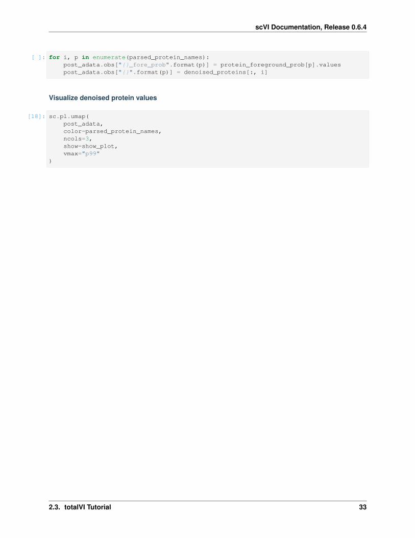
Visualize denoised protein values
[18]: sc.pl.umap(post_adata,color=parsed_protein_names,ncols=3,show=show_plot,vmax="p99"
)
2.3. totalVI Tutorial 33

scVI Documentation, Release 0.6.4
Visualize probability of foreground
Here we visualize the probability of foreground for each protein and cell (projected on UMAP). Some proteins areeasier to disentangle than others. Some proteins end up being “all background”. For example, CD15 does not appearto be captured well, when looking at the denoised values above we see no localization in the monocytes.
[15]: sc.pl.umap(post_adata,color=["{}_fore_prob".format(p) for p in parsed_protein_names],ncols=3,
(continues on next page)
34 Chapter 2. Tutorials

scVI Documentation, Release 0.6.4
(continued from previous page)
show=show_plot,)
For example, CD25 appears to have a lot of overlap between background and foreground in the histogram of log UMI,which is why we see greater uncertainty in the respective CD25 UMAP above.
[16]: _ = plt.hist(np.log(
dataset.protein_expression[:, np.where(dataset.protein_names == "CD25_TotalSeqB")[0]
]
(continues on next page)
2.3. totalVI Tutorial 35

scVI Documentation, Release 0.6.4
(continued from previous page)
+ 1),bins=50,
)plt.title("CD25 Log Counts")plt.ylabel("Number of cells")
[16]: Text(0, 0.5, 'Number of cells')
[ ]:
2.4 Harmonizing data with scVI and scANVI
[ ]: # If running in Colab, navigate to Runtime -> Change runtime type# and ensure you're using a Python 3 runtime with GPU hardware accelerator# installation in Colab can take several minutes
[ ]: import sysIN_COLAB = "google.colab" in sys.modules
def allow_notebook_for_test():print("Testing the harmonization notebook")
show_plot = Truetest_mode = Falsesave_path = "data/"
if IN_COLAB:!pip install --quiet git+https://github.com/yoseflab/scvi@stable
→˓#egg=scvi[notebooks]
[ ]: import matplotlibmatplotlib.rcParams["pdf.fonttype"] = 42
(continues on next page)
36 Chapter 2. Tutorials

scVI Documentation, Release 0.6.4
(continued from previous page)
matplotlib.rcParams["ps.fonttype"] = 42import matplotlib.pyplot as pltfrom matplotlib.colors import LinearSegmentedColormapimport seaborn as sns
import numpy as npimport numpy.random as randomimport pandas as pdimport scanpy as scimport louvain
from scvi.dataset.dataset import GeneExpressionDatasetfrom scvi.inference import UnsupervisedTrainerfrom scvi.models import SCANVI, VAE
from umap import UMAP
# Control UMAP numba warningsimport warnings; warnings.simplefilter('ignore')
if IN_COLAB:%matplotlib inline
# Use GPUuse_cuda = True
The raw data is provided in the Seurat notebook and can be downloaded here
2.4.1 Introduction
This tutorial walks through the harmonization process, specifically making use of scVI and SCANVI, which are twotools that are applicable and useful for principled large-scale analysis of single-cell transcriptomics atlases. Dataharmonization refers to the integration of two or more transcriptomics dataset into a single dataset on which anydownstream analysis can be applied. The input datasets may come from very different sources and from samples witha different composition of cell types. scVI is a deep generative model that has been developed for probabilistic rep-resentation of scRNA-seq data and performs well in both harmonization and harmonization-based annotation, goingbeyond just correcting batch effects. SCANVI is a new method that is designed to harmonize datasets, while alsoexplicitly leveraging any available labels to achieve more accurate annotation. SCANVI uses a semi-supervised gen-erative model. The inference of both models (scVI, SCANVI) is done using neural networks, stochastic optimization,and variational inference and scales to millions of cells and multiple datasets. Furthermore, both methods provide acomplete probabilistic representation of the data, which non-linearly controls not only for sample-to-sample bias, butalso for other technical factors of variation such as over-dispersion, variable library size, and zero-inflation.
The following tutorial is designed to provide an overview of the data harmonization methods, scVI and SCANVI. Thistutorial runs through two examples: 1) Tabula Muris dataset and 2) Human dataset (Seurat) Goals: - Setting up anddownloading datasets - Performing data harmonization with scVI - Performing marker selection from differentaillyexpressed genes for each cluster - Performing differential expression within each cluster
2.4. Harmonizing data with scVI and scANVI 37

scVI Documentation, Release 0.6.4
Dataset loading
The cell below is used to load in two human PBMC dataset, one stimulated and one control.
[4]: download_data = Falseif IN_COLAB or download_data:
!mkdir data!wget https://www.dropbox.com/s/79q6dttg8yl20zg/immune_alignment_expression_
→˓matrices.zip?dl=1 -O data/immune_alignment_expression_matrices.zip!cd data; unzip immune_alignment_expression_matrices.zip
mkdir: cannot create directory ‘data’: File exists--2019-12-28 18:58:55-- https://www.dropbox.com/s/79q6dttg8yl20zg/immune_alignment_→˓expression_matrices.zip?dl=1Resolving www.dropbox.com (www.dropbox.com)... 162.125.8.1, 2620:100:6016:1::a27d:101Connecting to www.dropbox.com (www.dropbox.com)|162.125.8.1|:443... connected.HTTP request sent, awaiting response... 301 Moved PermanentlyLocation: /s/dl/79q6dttg8yl20zg/immune_alignment_expression_matrices.zip [following]--2019-12-28 18:58:55-- https://www.dropbox.com/s/dl/79q6dttg8yl20zg/immune_→˓alignment_expression_matrices.zipReusing existing connection to www.dropbox.com:443.HTTP request sent, awaiting response... 302 FoundLocation: https://uc1403acf060990a493fabdccbe5.dl.dropboxusercontent.com/cd/0/get/→˓AvHUyrRQSPsh74XfdrAlCWOZSP4kPB0wvXSnuxJLlgj6apM0OtsnlR2yc1yjRznYyz0cztcOSreiw7S-→˓rIjTfYitOGst7j6Tg5wsQztOufg3QA/file?dl=1# [following]--2019-12-28 18:58:56-- https://uc1403acf060990a493fabdccbe5.dl.dropboxusercontent.→˓com/cd/0/get/→˓AvHUyrRQSPsh74XfdrAlCWOZSP4kPB0wvXSnuxJLlgj6apM0OtsnlR2yc1yjRznYyz0cztcOSreiw7S-→˓rIjTfYitOGst7j6Tg5wsQztOufg3QA/file?dl=1Resolving uc1403acf060990a493fabdccbe5.dl.dropboxusercontent.com→˓(uc1403acf060990a493fabdccbe5.dl.dropboxusercontent.com)... 162.125.8.6, 2620:100:→˓6016:6::a27d:106Connecting to uc1403acf060990a493fabdccbe5.dl.dropboxusercontent.com→˓(uc1403acf060990a493fabdccbe5.dl.dropboxusercontent.com)|162.125.8.6|:443...→˓connected.HTTP request sent, awaiting response... 200 OKLength: 21329741 (20M) [application/binary]Saving to: ‘data/immune_alignment_expression_matrices.zip’
data/immune_alignme 100%[===================>] 20.34M 38.3MB/s in 0.5s
2019-12-28 18:58:57 (38.3 MB/s) - ‘data/immune_alignment_expression_matrices.zip’→˓saved [21329741/21329741]
Archive: immune_alignment_expression_matrices.zipreplace immune_control_expression_matrix.txt.gz? [y]es, [n]o, [A]ll, [N]one, [r]ename:
[5]: # This can take several minutesfrom scvi.dataset.csv import CsvDatasetfilename = 'immune_stimulated_expression_matrix.txt.gz' if IN_COLAB else 'immune_→˓stimulated_expression_matrix.txt'stimulated = CsvDataset(filename=filename,
save_path=save_path,sep='\t', new_n_genes=35635,compression="gzip" if IN_COLAB else None)
filename = 'immune_control_expression_matrix.txt.gz' if IN_COLAB else 'immune_control_→˓expression_matrix.txt'control = CsvDataset(filename=filename,
save_path=save_path, sep='\t', new_n_genes=35635,
(continues on next page)
38 Chapter 2. Tutorials
scVI Documentation, Release 0.6.4
(continued from previous page)
compression="gzip" if IN_COLAB else None)
[2019-12-28 19:01:13,912] INFO - scvi.dataset.csv | Preprocessing dataset[2019-12-28 19:02:53,857] INFO - scvi.dataset.csv | Finished preprocessing dataset[2019-12-28 19:02:56,328] INFO - scvi.dataset.dataset | Remapping labels to [0,N][2019-12-28 19:02:56,330] INFO - scvi.dataset.dataset | Remapping batch_indices to [0,→˓N][2019-12-28 19:02:56,912] INFO - scvi.dataset.dataset | Computing the library size→˓for the new data[2019-12-28 19:02:57,473] INFO - scvi.dataset.dataset | Downsampled from 12875 to→˓12875 cells[2019-12-28 19:02:57,476] INFO - scvi.dataset.dataset | Not subsampling. Expecting: 1→˓< (new_n_genes=35635) <= self.nb_genes[2019-12-28 19:02:57,477] INFO - scvi.dataset.csv | Preprocessing dataset[2019-12-28 19:04:39,096] INFO - scvi.dataset.csv | Finished preprocessing dataset[2019-12-28 19:04:43,433] INFO - scvi.dataset.dataset | Remapping labels to [0,N][2019-12-28 19:04:43,435] INFO - scvi.dataset.dataset | Remapping batch_indices to [0,→˓N][2019-12-28 19:04:44,081] INFO - scvi.dataset.dataset | Computing the library size→˓for the new data[2019-12-28 19:04:44,657] INFO - scvi.dataset.dataset | Downsampled from 13019 to→˓13019 cells[2019-12-28 19:04:44,673] INFO - scvi.dataset.dataset | Not subsampling. Expecting: 1→˓< (new_n_genes=35635) <= self.nb_genes
[6]: # We subsample genes here so that computation works in Colabif IN_COLAB:
stimulated.subsample_genes(5000)control.subsample_genes(5000)
[2019-12-28 19:04:44,680] INFO - scvi.dataset.dataset | extracting highly variable→˓genes
Transforming to str index./usr/local/lib/python3.6/dist-packages/scanpy/preprocessing/_simple.py:284:→˓DeprecationWarning: Use is_view instead of isview, isview will be removed in the→˓future.if isinstance(data, AnnData) and data.isview:
[2019-12-28 19:04:52,645] INFO - scvi.dataset.dataset | Downsampling from 35635 to→˓5000 genes[2019-12-28 19:04:53,295] INFO - scvi.dataset.dataset | Computing the library size→˓for the new data[2019-12-28 19:04:53,936] INFO - scvi.dataset.dataset | Filtering non-expressing→˓cells.[2019-12-28 19:04:54,581] INFO - scvi.dataset.dataset | Computing the library size→˓for the new data[2019-12-28 19:04:54,685] INFO - scvi.dataset.dataset | Downsampled from 12875 to→˓12875 cells[2019-12-28 19:04:54,686] INFO - scvi.dataset.dataset | extracting highly variable→˓genes
Transforming to str index./usr/local/lib/python3.6/dist-packages/scanpy/preprocessing/_simple.py:284:→˓DeprecationWarning: Use is_view instead of isview, isview will be removed in the→˓future.if isinstance(data, AnnData) and data.isview:
2.4. Harmonizing data with scVI and scANVI 39

scVI Documentation, Release 0.6.4
[2019-12-28 19:05:03,599] INFO - scvi.dataset.dataset | Downsampling from 35635 to→˓5000 genes[2019-12-28 19:05:04,961] INFO - scvi.dataset.dataset | Computing the library size→˓for the new data[2019-12-28 19:05:05,156] INFO - scvi.dataset.dataset | Filtering non-expressing→˓cells.[2019-12-28 19:05:05,331] INFO - scvi.dataset.dataset | Computing the library size→˓for the new data[2019-12-28 19:05:05,416] INFO - scvi.dataset.dataset | Downsampled from 13019 to→˓13019 cells
2.4.2 Concatenate Datasets
[7]: all_dataset = GeneExpressionDataset()all_dataset.populate_from_datasets([control, stimulated])
[2019-12-28 19:05:05,435] INFO - scvi.dataset.dataset | Keeping 2140 genes[2019-12-28 19:05:05,663] INFO - scvi.dataset.dataset | Computing the library size→˓for the new data[2019-12-28 19:05:05,992] INFO - scvi.dataset.dataset | Remapping labels to [0,N][2019-12-28 19:05:05,994] INFO - scvi.dataset.dataset | Remapping batch_indices to [0,→˓N][2019-12-28 19:05:06,087] INFO - scvi.dataset.dataset | Computing the library size→˓for the new data[2019-12-28 19:05:06,175] INFO - scvi.dataset.dataset | Remapping labels to [0,N][2019-12-28 19:05:06,177] INFO - scvi.dataset.dataset | Remapping batch_indices to [0,→˓N][2019-12-28 19:05:06,421] INFO - scvi.dataset.dataset | Remapping labels to [0,N][2019-12-28 19:05:06,424] INFO - scvi.dataset.dataset | Remapping batch_indices to [0,→˓N]
2.4.3 scVI (single-cell Variational Inference)
*scVI* is a hierarchical Bayesian model for single-cell RNA sequencing data with conditional distributionsparametrized by neural networks. Working as a hybrid between a neural network and a bayesian network, scVIperforms data harmonization. VAE refers to variational auto-encoders for single-cell gene expression data. scVI issimilar to VAE as it tries to bring a more suitable structure to the latent space. While VAE allows users to makeobservations in a semi-supervised fashion, scVI is easier to train and specific cell-type labels for the dataset are notrequired in the pure unsupervised case.
Define the scVI model
• First, we define the model and its hyperparameters:
– n_hidden: number of units in the hidden layer = 128
– n_latent: number of dimensions in the shared latent space = 10 (how many dimensions in z)
– n_layers: number of layers in the neural network
– dispersion: ‘gene’: each gene has its own dispersion parameter; ‘gene-batch’: each gene in each batchhas its own dispersion parameter
• Then, we define a trainer using the model and the dataset to train it with
40 Chapter 2. Tutorials

scVI Documentation, Release 0.6.4
– in the unsupervised setting, train_size=1.0 and all cells are used for training
[8]: vae = VAE(all_dataset.nb_genes, n_batch=all_dataset.n_batches, n_labels=all_dataset.n_→˓labels,
n_hidden=128, n_latent=30, n_layers=2, dispersion='gene')
trainer = UnsupervisedTrainer(vae, all_dataset, train_size=1.0)n_epochs = 100trainer.train(n_epochs=n_epochs)
HBox(children=(FloatProgress(value=0.0, description='training',→˓style=ProgressStyle(description_width='initial...
2.4.4 Train the vae model for 100 epochs (this should take apporximately 12 min-utes on a GPU)
If it is desired to save to model and take on the downstream analysis later, save the model, and comment outtrainer.train(). Use the saved model to ensure that the down stream analysis cluster id are identical, but the resultis robust to reruns of the model, although the exact numerical ids of the clusters might change
[1]: # trainer.train(n_epochs=100)# torch.save(trainer.model.state_dict(),save_path+'harmonization.vae.allgenes.30.→˓model.pkl')
[ ]: # trainer.model.load_state_dict(torch.load(save_path+'harmonization.vae.allgenes.30.→˓model.pkl'))# trainer.model.eval()
2.4.5 Visualize the latent space
The latent space representation of the cells provides a way to address the harmonization problem, as allthe cells are projected onto a joint latent space, inferred while controlling for their dataset of origin.
Obtain the latent space from the posterior object
First, the posterior object is obtained by providing the model that was trained on the dataset. Then, thelatent space along with the labels is obtained.
[ ]: full = trainer.create_posterior(trainer.model, all_dataset, indices=np.arange(len(all_→˓dataset)))latent, batch_indices, labels = full.sequential().get_latent()batch_indices = batch_indices.ravel()
2.4. Harmonizing data with scVI and scANVI 41

scVI Documentation, Release 0.6.4
Use UMAP to generate 2D visualization
[ ]: latent_u = UMAP(spread=2).fit_transform(latent)
Plot data colored by batch
[37]: cm = LinearSegmentedColormap.from_list('my_cm', ['deepskyblue', 'hotpink'], N=2)
fig, ax = plt.subplots(figsize=(5, 5))order = np.arange(latent.shape[0])random.shuffle(order)ax.scatter(latent_u[order, 0], latent_u[order, 1],
c=all_dataset.batch_indices.ravel()[order],cmap=cm, edgecolors='none', s=5)
plt.axis("off")fig.set_tight_layout(True)
[13]: adata_latent = sc.AnnData(latent)sc.pp.neighbors(adata_latent, use_rep='X', n_neighbors=30, metric='minkowski')sc.tl.louvain(adata_latent, partition_type=louvain.ModularityVertexPartition, use_→˓weights=False)clusters = adata_latent.obs.louvain.values.to_dense().astype(int)
/usr/local/lib/python3.6/dist-packages/scanpy/neighbors/__init__.py:89:→˓DeprecationWarning: Use is_view instead of isview, isview will be removed in the→˓future.if adata.isview: # we shouldn't need this here...
42 Chapter 2. Tutorials

scVI Documentation, Release 0.6.4
plot clusters in 2D UMAP
[14]: colors = ["#991f1f", "#ff9999", "#ff4400", "#ff8800", "#664014", "#665c52","#cca300", "#f1ff33", "#b4cca3", "#0e6600", "#33ff4e", "#00ccbe","#0088ff", "#7aa6cc", "#293966", "#0000ff", "#9352cc", "#cca3c9", "#cc2996"]
fig = plt.figure(figsize=(7, 7), facecolor='w', edgecolor='k')for i, k in enumerate(np.unique(clusters)):
plt.scatter(latent_u[clusters == k, 0], latent_u[clusters == k, 1], label=k,edgecolors='none', c=colors[k], s=5)
plt.legend(borderaxespad=0, fontsize='large', markerscale=5)
plt.axis('off')fig.set_tight_layout(True)
Generate list of genes that is enriched for higher expression in cluster 𝑖 compared to all other clusters
Here we compare the gene expression in cells from one cluster to all the other cells by * sampling mean parameterfrom the scVI ZINB model * compare pairs of cells from one subset v.s. the other * compute bayes factor based onthe number of times the cell from the cluster of interest has a higher expression * generate DE genelist ranked by thebayes factor
2.4. Harmonizing data with scVI and scANVI 43

scVI Documentation, Release 0.6.4
[15]: # change to output_file=True to get an Excel file with all DE informationde_res, de_clust = full.one_vs_all_degenes(cell_labels=clusters, n_samples=10000,
M_permutation=10000, output_file=False,save_dir=save_path, filename='Harmonized_
→˓ClusterDE',min_cells=1)
# with open(save_path+'Harmonized_ClusterDE.pkl', 'wb') as f:# pickle.dump((de_res, de_clust), f)
# with open(save_path+'Harmonized_ClusterDE.pkl', 'rb') as f:# de_res, de_clust = pickle.load(f)
HBox(children=(FloatProgress(value=0.0, max=12.0), HTML(value='')))
2.4.6 Find markers for each cluster
absthres is the minimum average number of UMI in the cluster of interest to be a marker gene
relthres is the minimum fold change in number of UMI in the cluster of interest compared to all other cells for adifferentially expressed gene to be a marker gene
[ ]: def find_markers(deres, absthres, relthres, ngenes):allgenes = []for i, x in enumerate(deres):
markers = x.loc[(x["raw_mean1"] > absthres)& (x["raw_normalized_mean1"] / x["raw_normalized_mean2"] > relthres)
]if len(markers > 0):
ngenes = np.min([len(markers), ngenes])markers = markers[:ngenes]allgenes.append(markers)
if len(allgenes) > 0:markers = pd.concat(allgenes)return markers
else:return pd.DataFrame(
columns=["bayes_factor", "raw_mean1", "raw_mean2", "scale1", "scale2",→˓"clusters"]
)
[ ]: clustermarkers = find_markers(de_res, absthres=0.5, relthres=2, ngenes=3)
[18]: clustermarkers[['bayes_factor', 'raw_mean1', 'raw_mean2', 'scale1', 'scale2',→˓'clusters']]
[18]: bayes_factor raw_mean1 raw_mean2 scale1 scale2 clustersCCR7 2.407534 3.013568 1.101134 0.013815 0.003587 0LTB 2.268095 1.777387 0.487352 0.007570 0.001843 0IL7R 1.927748 0.634673 0.311735 0.003167 0.001115 0CCL2 5.595713 26.253246 0.228723 0.029112 0.000589 1
(continues on next page)
44 Chapter 2. Tutorials

scVI Documentation, Release 0.6.4
(continued from previous page)
CCL7 5.355480 4.972349 0.028503 0.005568 0.000125 1FTL 5.144079 176.007248 9.275810 0.187290 0.019729 1TRAT1 1.910720 0.653896 0.167326 0.002602 0.000722 2PABPC1 1.658972 6.917166 3.106116 0.023507 0.009658 2RGS1 1.650806 0.530394 0.202526 0.002463 0.000919 2MS4A1 5.651483 0.748272 0.006394 0.003434 0.000098 3CD74 4.321956 12.331393 3.460445 0.050822 0.004496 3CD79A 3.789829 1.613314 0.015208 0.007280 0.000794 3GZMH 4.240211 1.417158 0.055849 0.007224 0.000430 4LAG3 3.569430 0.623592 0.042574 0.003228 0.000483 4CCL5 3.305001 6.503485 0.693329 0.034972 0.004145 4GNLY 5.076985 15.870968 0.383623 0.075233 0.003782 5CLIC3 4.138269 1.343548 0.044229 0.005892 0.000413 5PRF1 3.866617 1.969355 0.088208 0.007446 0.000490 5MS4A7 6.375420 7.652462 0.322973 0.007434 0.000704 6FCGR3A 5.651483 8.363636 0.207947 0.009378 0.000555 6VMO1 5.215940 7.813447 0.061599 0.010655 0.000418 6SRSF2 4.261868 1.669421 0.208488 0.005357 0.000696 7RSRC2 4.254598 1.007084 0.114545 0.003176 0.000410 7EIF5 4.157867 1.731995 0.517148 0.005871 0.001542 7HLA-DRA 4.747355 83.215843 3.797282 0.066441 0.007408 8CST3 4.724163 17.680328 1.295479 0.012285 0.001606 8HLA-DPB1 4.436397 30.666666 1.030555 0.022211 0.002274 8HBB 18.420681 1517.298096 0.327821 0.298531 0.000602 9HBA2 18.420681 412.360779 0.073131 0.266350 0.000510 9HBA1 18.420681 221.607849 0.039393 0.188938 0.000401 9PPBP 5.651483 11.469768 0.105767 0.034214 0.000672 10SDPR 5.355480 1.758139 0.017952 0.005284 0.000207 10TUBB1 5.313606 1.120930 0.007944 0.004412 0.000108 10MYBL2 7.823621 0.750000 0.000271 0.001742 0.000011 11TSPAN13 7.823621 5.953704 0.014775 0.011108 0.000114 11CCL19 6.375420 0.787037 0.000582 0.002303 0.000030 11
2.4.7 Plotting known cluster unique genes
[ ]: Markers = ["CD3D", "SELL", "CREM", "CD8B", "GNLY", "CD79A", "FCGR3A", "CCL2", "PPBP"]
[ ]: def plot_marker_genes(latent_u, count, genenames, markers):nrow = (len(markers) // 3 + 1)figh = nrow * 4fig = plt.figure(figsize=(10, figh))for i, x in enumerate(markers):
if np.sum(genenames == x)==1:exprs = count[:, genenames == x].ravel()idx = (exprs > 0)plt.subplot(nrow, 3, (i + 1))plt.scatter(latent_u[:, 0], latent_u[:, 1], c='lightgrey', edgecolors=
→˓'none', s=5)plt.scatter(latent_u[idx, 0], latent_u[idx, 1], c=exprs[idx], cmap=plt.
→˓get_cmap('viridis_r'),edgecolors='none', s=3)
plt.title(x)fig.set_tight_layout(True)
2.4. Harmonizing data with scVI and scANVI 45
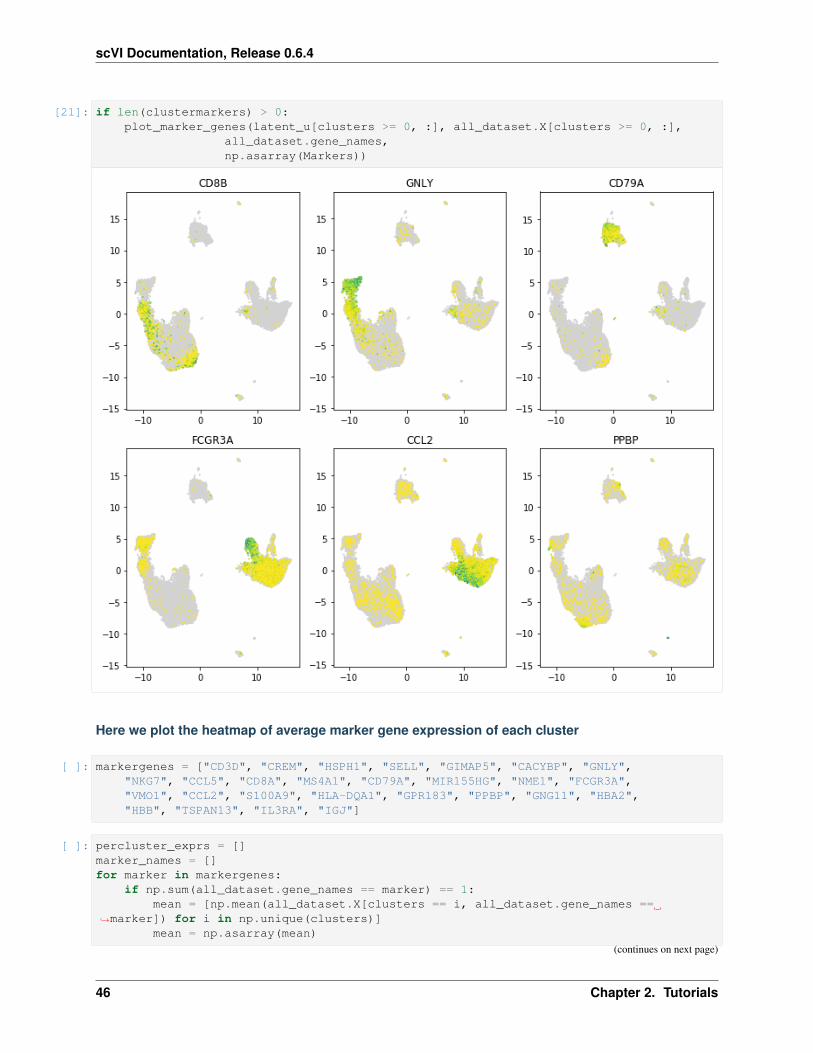
scVI Documentation, Release 0.6.4
[21]: if len(clustermarkers) > 0:plot_marker_genes(latent_u[clusters >= 0, :], all_dataset.X[clusters >= 0, :],
all_dataset.gene_names,np.asarray(Markers))
Here we plot the heatmap of average marker gene expression of each cluster
[ ]: markergenes = ["CD3D", "CREM", "HSPH1", "SELL", "GIMAP5", "CACYBP", "GNLY","NKG7", "CCL5", "CD8A", "MS4A1", "CD79A", "MIR155HG", "NME1", "FCGR3A","VMO1", "CCL2", "S100A9", "HLA-DQA1", "GPR183", "PPBP", "GNG11", "HBA2","HBB", "TSPAN13", "IL3RA", "IGJ"]
[ ]: percluster_exprs = []marker_names = []for marker in markergenes:
if np.sum(all_dataset.gene_names == marker) == 1:mean = [np.mean(all_dataset.X[clusters == i, all_dataset.gene_names ==
→˓marker]) for i in np.unique(clusters)]mean = np.asarray(mean)
(continues on next page)
46 Chapter 2. Tutorials

scVI Documentation, Release 0.6.4
(continued from previous page)
percluster_exprs.append(np.log10(mean / np.mean(mean) + 1))marker_names.append(marker)
[24]: if len(percluster_exprs) > 0:percluster_exprs = pd.DataFrame(percluster_exprs, index=marker_names)sns.clustermap(percluster_exprs, row_cluster=False, col_cluster=True)
2.4. Harmonizing data with scVI and scANVI 47

scVI Documentation, Release 0.6.4
2.4.8 Plotting scVI discovered marker genes
Each row contains the top 3 marker gene expression of its corresponding cluster
[25]: plot_marker_genes(latent_u[clusters >= 0, :], all_dataset.X[clusters >= 0, :],all_dataset.gene_names, np.asarray(clustermarkers.index))
48 Chapter 2. Tutorials

scVI Documentation, Release 0.6.4
2.4. Harmonizing data with scVI and scANVI 49

scVI Documentation, Release 0.6.4
2.4.9 Compare list of genes that are differentially expressed in each clusters
[ ]: # change to output_file=True to get an Excel file with all DE informationde_res_stim, de_clust_stim = full.within_cluster_degenes(cell_labels=clusters,
states=all_dataset.batch_→˓indices.ravel() == 1,
output_file=False,→˓batch1=[1], batch2=[0],
save_dir=save_path, filename=→˓'Harmonized_StimDE',
min_cells=1)
# with open(save_path+'Harmonized_StimDE.pkl', 'wb') as f:# pickle.dump((de_res_stim,de_clust_stim), f)
# with open(save_path+'Harmonized_StimDE.pkl', 'rb') as f:# de_res_stim,de_clust_stim = pickle.load(f)
[ ]: genelist = []for i, x in enumerate(de_clust_stim):
de = de_res_stim[i].loc[de_res_stim[i]["raw_mean1"] > 1]de = de.loc[de["bayes_factor"] > 2]if len(de) > 0:
de["cluster"] = np.repeat(x, len(de))genelist.append(de)
if len(genelist) > 0:genelist = pd.concat(genelist)genelist["genenames"] = list(genelist.index)degenes, nclusterde = np.unique(genelist.index, return_counts=True)
Genes that are differentially expressed in at least 10 of the clusters
[28]: if len(genelist) > 0:print(", ".join(degenes[nclusterde > 11]))
C15ORF48, C3AR1, CCL2, CST3, SAT1, TXN, TXNIP, TYROBP
[ ]: if len(genelist) > 0:cluster0shared = genelist.loc[genelist['genenames'].isin(degenes[nclusterde >
→˓10])]cluster0shared = cluster0shared.loc[cluster0shared['cluster'] == 0]
[ ]: def plot_marker_genes_compare(latent_u, count, genenames, markers, subset):nrow = len(markers)figh = nrow * 4fig = plt.figure(figsize=(8, figh))notsubset = np.asarray([not x for x in subset])for i, x in enumerate(markers):
if np.sum(genenames == x) == 1:exprs = count[:, genenames == x].ravel()idx = (exprs > 0)plt.subplot(nrow, 2, (i * 2 + 1))
(continues on next page)
50 Chapter 2. Tutorials

scVI Documentation, Release 0.6.4
(continued from previous page)
plt.scatter(latent_u[subset, 0], latent_u[subset, 1], c='lightgrey',→˓edgecolors='none', s=5)
plt.scatter(latent_u[idx, 0][subset[idx]], latent_u[idx, 1][subset[idx]],→˓c=exprs[idx][subset[idx]],
cmap=plt.get_cmap('viridis_r'), edgecolors='none', s=3)plt.title(x + ' control')fig.set_tight_layout(True)plt.subplot(nrow, 2, (i * 2 + 2))plt.scatter(latent_u[notsubset, 0], latent_u[notsubset, 1], c='lightgrey',
→˓ edgecolors='none', s=5)plt.scatter(latent_u[idx, 0][notsubset[idx]], latent_u[idx,
→˓1][notsubset[idx]],c=exprs[idx][notsubset[idx]], cmap=plt.get_cmap('viridis_r'),
→˓edgecolors='none', s=3)plt.title(x + ' stimulated')
[31]: plot_marker_genes_compare(latent_u, all_dataset.X, all_dataset.gene_names,["CD3D", "GNLY", "IFI6", "ISG15", "CD14", "CXCL10"], batch_
→˓indices == 0)
2.4. Harmonizing data with scVI and scANVI 51
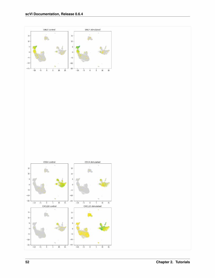
scVI Documentation, Release 0.6.4
52 Chapter 2. Tutorials

scVI Documentation, Release 0.6.4
[32]: if len(genelist) > 0:plot_marker_genes_compare(latent_u, all_dataset.X,
all_dataset.gene_names, cluster0shared.index,batch_indices == 0)
2.4. Harmonizing data with scVI and scANVI 53
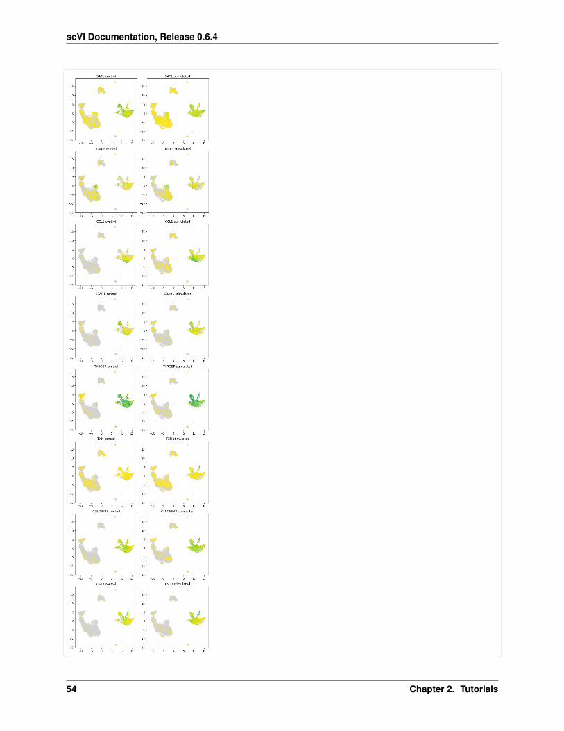
scVI Documentation, Release 0.6.4
54 Chapter 2. Tutorials

scVI Documentation, Release 0.6.4
Genes that are differentially expressed in one single cluster
[35]: if len(genelist) > 0 and len(nclusterde) > 0:degenes[nclusterde == 1]clusteruniq = genelist.loc[genelist['genenames'].isin(degenes[nclusterde == 1])]clusteruniq = clusteruniq.loc[clusteruniq['cluster'] == 3]plot_marker_genes_compare(latent_u, all_dataset.X, all_dataset.gene_names,
→˓clusteruniq.index, batch_indices == 0)
<Figure size 576x0 with 0 Axes>
[ ]:
2.5 Clustering 3K PBMCs with scVI and ScanPy
Disclaimer: some of the code in this notebook was taken from Scanpy’s Clustering tutorial (https://scanpy-tutorials.readthedocs.io/en/latest/pbmc3k.html) which is itself based on SEURAT’s clustering tutorial in R.
This notebook is designed as a demonstration of scVI’s potency on the tasks considered in the Scanpy PBMC 3KClustering notebook. In order to do so, we follow the same workflow adopted by scanpy in their clustering tutorialwhile performing the analysis using scVI as often as possible. Specifically, we use scVI’s latent representation anddifferential expression analysis (which computes a Bayes Factor on imputed values). For visualisation, pre-processingand for some canonical analysis, we use the Scanpy package directly.
When useful, we provide high-level wrappers around scVI’s analysis tools. These functions are designed to makestandard use of scVI as easy as possible. For specific use cases, we encourage the reader to take a closer look at thosefunctions and modify them according to their needs.
[ ]: # If running in Colab, navigate to Runtime -> Change runtime type# and ensure you're using a Python 3 runtime with GPU hardware accelerator# installation in Colab can take several minutes
2.5.1 Colab and automated testing configuration
[1]: def allow_notebook_for_test():print("Testing the scanpy pbmc3k notebook")
import sys, os
n_epochs_all = Nonetest_mode = Falseshow_plot = True
def if_not_test_else(x, y):if not test_mode:
return xelse:
return y
IN_COLAB = "google.colab" in sys.modules
(continues on next page)
2.5. Clustering 3K PBMCs with scVI and ScanPy 55
scVI Documentation, Release 0.6.4
(continued from previous page)
show_plot = Truetest_mode = Falsen_epochs_all = Nonesave_path = "data/"
if not test_mode and not IN_COLAB:save_path = "../../data"
if IN_COLAB:!pip install --quiet git+https://github.com/yoseflab/scvi@stable
→˓#egg=scvi[notebooks]
2.5.2 Initialization
[2]: download_data = Falseif IN_COLAB or download_data:
!mkdir data!wget http://cf.10xgenomics.com/samples/cell-exp/1.1.0/pbmc3k/pbmc3k_filtered_
→˓gene_bc_matrices.tar.gz -O data/pbmc3k_filtered_gene_bc_matrices.tar.gz!cd data; tar -xzf pbmc3k_filtered_gene_bc_matrices.tar.gz
[3]: # Seed for reproducibilityimport torchimport numpy as npimport pandas as pdimport scanpy as scfrom typing import Tuple
# scVI importsimport scvifrom scvi.dataset import AnnDatasetFromAnnDatafrom scvi.inference import UnsupervisedTrainerfrom scvi.models.vae import VAE
torch.manual_seed(0)np.random.seed(0)sc.settings.verbosity = 0 # verbosity: errors (0), warnings (1), info (2), hints (3)
[5]: if not test_mode:sc.settings.set_figure_params(dpi=60)%matplotlib inline
[6]: # Load the dataadata = sc.read_10x_mtx(
os.path.join(save_path, "filtered_gene_bc_matrices/hg19/"
), # the directory with the `.mtx` filevar_names="gene_symbols", # use gene symbols for the variable names (variables-
→˓axis index))adata.var_names_make_unique()
56 Chapter 2. Tutorials

scVI Documentation, Release 0.6.4
2.5.3 Preprocessing
In the following section, we reproduce the preprocessing steps adopted in the scanpy notebook.
Basic filtering: we remove cells with a low number of genes expressed and genes which are expressed in a low numberof cells.
[7]: min_genes = if_not_test_else(200, 0)min_cells = if_not_test_else(3, 0)
[8]: sc.settings.verbosity = 2sc.pp.filter_cells(adata, min_genes=min_genes)sc.pp.filter_genes(adata, min_cells=min_cells)sc.pp.filter_cells(adata, min_genes=1)
filtered out 19024 genes that are detected in less than 3 cells
As in the scanpy notebook, we then look for high levels of mitochondrial genes and high number of expressed geneswhich are indicators of poor quality cells.
[9]: mito_genes = adata.var_names.str.startswith("MT-")adata.obs["percent_mito"] = (
np.sum(adata[:, mito_genes].X, axis=1).A1 / np.sum(adata.X, axis=1).A1)adata.obs["n_counts"] = adata.X.sum(axis=1).A1
[10]: adata = adata[adata.obs["n_genes"] < 2500, :]adata = adata[adata.obs["percent_mito"] < 0.05, :]
2.5.4 scVI uses non normalized data so we keep the original data in a separateAnnData object, then the normalization steps are performed
Normalization and more filtering
We only keep highly variable genes
[11]: adata_original = adata.copy()
sc.pp.normalize_per_cell(adata, counts_per_cell_after=1e4)sc.pp.log1p(adata)
min_mean = if_not_test_else(0.0125, -np.inf)max_mean = if_not_test_else(3, np.inf)min_disp = if_not_test_else(0.5, -np.inf)max_disp = if_not_test_else(None, np.inf)
sc.pp.highly_variable_genes(adata,min_mean=min_mean,max_mean=max_mean,min_disp=min_disp,max_disp=max_disp
)
(continues on next page)
2.5. Clustering 3K PBMCs with scVI and ScanPy 57

scVI Documentation, Release 0.6.4
(continued from previous page)
highly_variable_genes = adata.var["highly_variable"]adata = adata[:, highly_variable_genes]
adata.raw = adata
sc.pp.regress_out(adata, ["n_counts", "percent_mito"])sc.pp.scale(adata, max_value=10)
# Also filter the original adata genesadata_original = adata_original[:, highly_variable_genes]print("{} highly variable genes".format(highly_variable_genes.sum()))
regressing out ['n_counts', 'percent_mito']sparse input is densified and may lead to high memory usefinished (0:00:12.37)
1838
2.5.5 Compute the scVI latent space
Below we provide then use a wrapper function designed to compute scVI’s latent representation of the non-normalizeddata. Specifically, we train scVI’s VAE, compute and store the latent representation then return the posterior whichwill later be used for further inference.
[12]: def compute_scvi_latent(adata: sc.AnnData,n_latent: int = 5,n_epochs: int = 100,lr: float = 1e-3,use_batches: bool = False,use_cuda: bool = False,
) -> Tuple[scvi.inference.Posterior, np.ndarray]:"""Train and return a scVI model and sample a latent space
:param adata: sc.AnnData object non-normalized:param n_latent: dimension of the latent space:param n_epochs: number of training epochs:param lr: learning rate:param use_batches:param use_cuda:return: (scvi.Posterior, latent_space)"""# Convert easily to scvi datasetscviDataset = AnnDatasetFromAnnData(adata)
# Train a modelvae = VAE(
scviDataset.nb_genes,n_batch=scviDataset.n_batches * use_batches,n_latent=n_latent,
)trainer = UnsupervisedTrainer(vae, scviDataset, train_size=1.0, use_cuda=use_cuda)trainer.train(n_epochs=n_epochs, lr=lr)####
# Extract latent space
(continues on next page)
58 Chapter 2. Tutorials

scVI Documentation, Release 0.6.4
(continued from previous page)
posterior = trainer.create_posterior(trainer.model, scviDataset, indices=np.arange(len(scviDataset))
).sequential()
latent, _, _ = posterior.get_latent()
return posterior, latent
[13]: n_epochs = 400 if n_epochs_all is None else n_epochs_all
# use_cuda to use GPUuse_cuda = True if IN_COLAB else False
scvi_posterior, scvi_latent = compute_scvi_latent(adata_original, n_epochs=n_epochs, n_latent=10, use_cuda=use_cuda
)adata.obsm["X_scvi"] = scvi_latent
# store scvi imputed expressionscale = scvi_posterior.get_sample_scale()for _ in range(9):
scale += scvi_posterior.get_sample_scale()scale /= 10
for gene, gene_scale in zip(adata.var.index, np.squeeze(scale).T):adata.obs["scale_" + gene] = gene_scale
training: 100%|| 10/10 [00:32<00:00, 3.21s/it]
2.5.6 Principal component analysis to reproduce ScanPy results and comparethem against scVI’s
Below, we reproduce exactly scanpy’s PCA on normalized data.
[14]: sc.tl.pca(adata, svd_solver="arpack")
[15]: sc.pl.pca(adata, color="CST3", show=show_plot)
2.5. Clustering 3K PBMCs with scVI and ScanPy 59

scVI Documentation, Release 0.6.4
[16]: sc.pl.pca_variance_ratio(adata, log=True, show=show_plot)
2.5.7 Computing, embedding and clustering the neighborhood graph
The Scanpy API computes a neighborhood graph with sc.pp.neighbors which can be called to work on a spe-cific representation use_rep='your rep'. Once the neighbors graph has been computed, all Scanpy algorithmsworking on it can be called as usual (that is louvain, paga, umap . . . )
[17]: sc.pp.neighbors(adata, n_neighbors=10, n_pcs=40)sc.tl.leiden(adata, key_added="leiden_pca")sc.tl.umap(adata)
computing neighborsusing 'X_pca' with n_pcs = 40finished (0:00:06.70)
(continues on next page)
60 Chapter 2. Tutorials
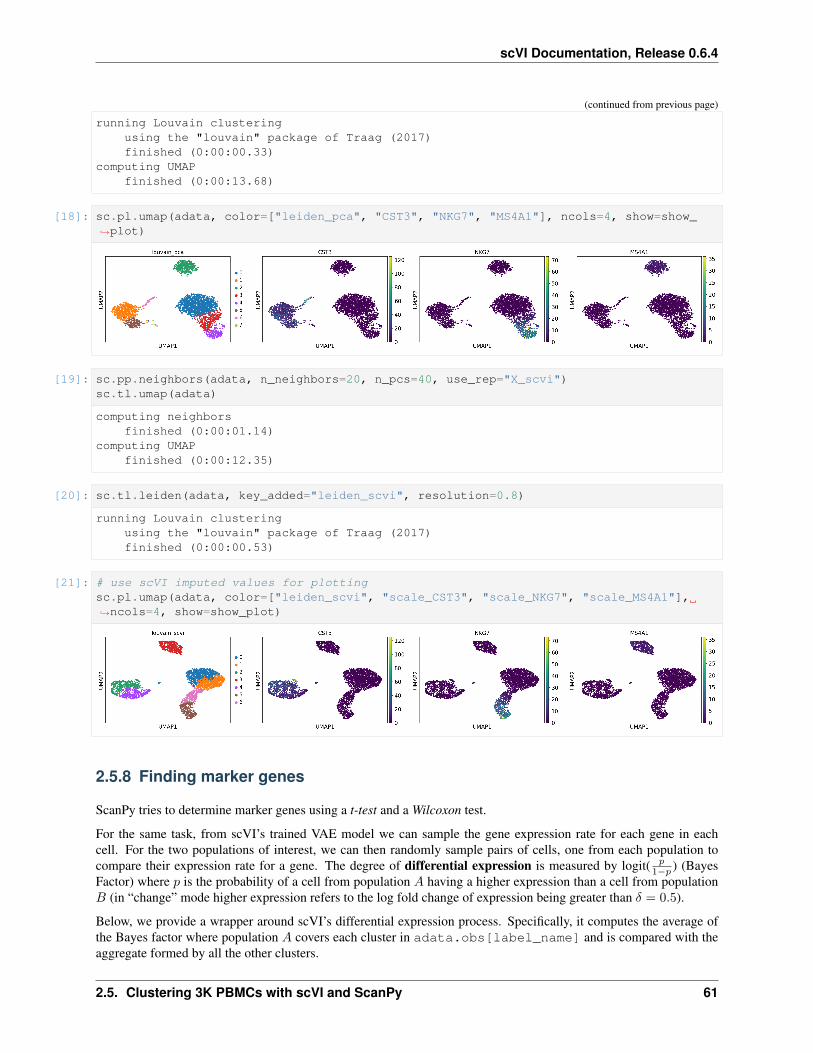
scVI Documentation, Release 0.6.4
(continued from previous page)
running Louvain clusteringusing the "louvain" package of Traag (2017)finished (0:00:00.33)
computing UMAPfinished (0:00:13.68)
[18]: sc.pl.umap(adata, color=["leiden_pca", "CST3", "NKG7", "MS4A1"], ncols=4, show=show_→˓plot)
[19]: sc.pp.neighbors(adata, n_neighbors=20, n_pcs=40, use_rep="X_scvi")sc.tl.umap(adata)
computing neighborsfinished (0:00:01.14)
computing UMAPfinished (0:00:12.35)
[20]: sc.tl.leiden(adata, key_added="leiden_scvi", resolution=0.8)
running Louvain clusteringusing the "louvain" package of Traag (2017)finished (0:00:00.53)
[21]: # use scVI imputed values for plottingsc.pl.umap(adata, color=["leiden_scvi", "scale_CST3", "scale_NKG7", "scale_MS4A1"],→˓ncols=4, show=show_plot)
2.5.8 Finding marker genes
ScanPy tries to determine marker genes using a t-test and a Wilcoxon test.
For the same task, from scVI’s trained VAE model we can sample the gene expression rate for each gene in eachcell. For the two populations of interest, we can then randomly sample pairs of cells, one from each population tocompare their expression rate for a gene. The degree of differential expression is measured by logit( 𝑝
1−𝑝 ) (BayesFactor) where 𝑝 is the probability of a cell from population 𝐴 having a higher expression than a cell from population𝐵 (in “change” mode higher expression refers to the log fold change of expression being greater than 𝛿 = 0.5).
Below, we provide a wrapper around scVI’s differential expression process. Specifically, it computes the average ofthe Bayes factor where population 𝐴 covers each cluster in adata.obs[label_name] and is compared with theaggregate formed by all the other clusters.
2.5. Clustering 3K PBMCs with scVI and ScanPy 61

scVI Documentation, Release 0.6.4
[22]: def rank_genes_groups_bayes(adata: sc.AnnData,scvi_posterior: scvi.inference.Posterior,n_samples: int = 5000,M_permutation: int = 10000,n_genes: int = 25,label_name: str = "leiden_scvi",mode: str = "vanilla"
) -> pd.DataFrame:"""Rank genes for characterizing groups.Computes Bayes factor for each cluster against the others to test for
→˓differential expression.See Nature article (https://rdcu.be/bdHYQ)
:param adata: sc.AnnData object non-normalized:param scvi_posterior::param n_samples::param M_permutation::param n_genes::param label_name: The groups tested are taken from adata.obs[label_name] which
→˓can be computedusing clustering like Louvain (Ex: sc.tl.louvain(adata, key_
→˓added=label_name) ):return: Summary of Bayes factor per gene, per cluster"""
# Call scvi functionper_cluster_de, cluster_id = scvi_posterior.one_vs_all_degenes(
cell_labels=np.asarray(adata.obs[label_name].values).astype(int).ravel(),min_cells=1,n_samples=n_samples,M_permutation=M_permutation,mode=mode
)
# convert to ScanPy format -- this is just about feeding scvi results into a→˓format readable by ScanPy
markers = []scores = []names = []for i, x in enumerate(per_cluster_de):
subset_de = x[:n_genes]markers.append(subset_de)scores.append(tuple(subset_de["bayes_factor"].values))names.append(tuple(subset_de.index.values))
markers = pd.concat(markers)dtypes_scores = [(str(i), "<f4") for i in range(len(scores))]dtypes_names = [(str(i), "<U50") for i in range(len(names))]scores = np.array([tuple(row) for row in np.array(scores).T], dtype=dtypes_scores)scores = scores.view(np.recarray)names = np.array([tuple(row) for row in np.array(names).T], dtype=dtypes_names)names = names.view(np.recarray)
adata.uns["rank_genes_groups_scvi"] = {"params": {
(continues on next page)
62 Chapter 2. Tutorials

scVI Documentation, Release 0.6.4
(continued from previous page)
"groupby": "","reference": "rest","method": "","use_raw": True,"corr_method": "",
},"scores": scores,"names": names,
}return markers
[23]: n_genes = 20sc.tl.rank_genes_groups(
adata,"leiden_scvi",method="t-test",use_raw=True,key_added="rank_genes_groups_ttest",n_genes=n_genes,
)sc.tl.rank_genes_groups(
adata,"leiden_scvi",method="wilcoxon",use_raw=True,key_added="rank_genes_groups_wilcox",n_genes=n_genes,
)sc.pl.rank_genes_groups(
adata, key="rank_genes_groups_ttest", sharey=False, n_genes=n_genes, show=show_→˓plot)sc.pl.rank_genes_groups(
adata, key="rank_genes_groups_wilcox", sharey=False, n_genes=n_genes, show=show_→˓plot)
ranking genesfinished (0:00:00.65)
ranking genesfinished (0:00:01.49)
2.5. Clustering 3K PBMCs with scVI and ScanPy 63

scVI Documentation, Release 0.6.4
[24]: rank_genes_groups_bayes(adata, scvi_posterior, label_name="leiden_scvi", n_genes=n_genes
)sc.pl.rank_genes_groups(
adata, key="rank_genes_groups_scvi", sharey=False, n_genes=n_genes, show=show_plot)
[25]: # We compute the rank of every gene to perform analysis afterall_genes = len(adata.var_names)
sc.tl.rank_genes_groups(adata, 'leiden_scvi', method='t-test', use_raw=False, key_→˓added='rank_genes_groups_ttest', n_genes=all_genes)sc.tl.rank_genes_groups(adata, 'leiden_scvi', method='wilcoxon', use_raw=False, key_→˓added='rank_genes_groups_wilcox', n_genes=all_genes)differential_expression = rank_genes_groups_bayes(adata, scvi_posterior, label_name=→˓'leiden_scvi', n_genes=all_genes)
ranking genesfinished (0:00:00.67)
ranking genesfinished (0:00:01.50)
[26]: def ratio(A, B):A, B = set(A), set(B)
(continues on next page)
64 Chapter 2. Tutorials

scVI Documentation, Release 0.6.4
(continued from previous page)
return len(A.intersection(B)) / len(A) * 100
[27]: cluster_distrib = adata.obs.groupby("leiden_scvi").count()["n_genes"]
For each cluster, we compute the percentage of genes which are in the n_genes most expressed genes of bothScanpy’s and scVI’s differential expression tests.
[28]: n_genes = 25
sc.pl.umap(adata, color=["leiden_scvi"], ncols=1, show=show_plot)for c in cluster_distrib.index:
print("Cluster %s (%d cells): t-test / wilcox %6.2f %% & t-test / scvi %6.2f %%"% (
c,cluster_distrib[c],ratio(
adata.uns["rank_genes_groups_ttest"]["names"][c][:n_genes],adata.uns["rank_genes_groups_wilcox"]["names"][c][:n_genes],
),ratio(
adata.uns["rank_genes_groups_ttest"]["names"][c][:n_genes],adata.uns["rank_genes_groups_scvi"]["names"][c][:n_genes],
),)
)
Cluster 0 (613 cells): t-test / wilcox 8.00 % & t-test / scvi 4.00 %Cluster 1 (526 cells): t-test / wilcox 28.00 % & t-test / scvi 40.00 %Cluster 2 (355 cells): t-test / wilcox 20.00 % & t-test / scvi 76.00 %Cluster 3 (345 cells): t-test / wilcox 64.00 % & t-test / scvi 40.00 %Cluster 4 (317 cells): t-test / wilcox 100.00 % & t-test / scvi 0.00 %Cluster 5 (254 cells): t-test / wilcox 76.00 % & t-test / scvi 40.00 %Cluster 6 (228 cells): t-test / wilcox 36.00 % & t-test / scvi 24.00 %
2.5. Clustering 3K PBMCs with scVI and ScanPy 65

scVI Documentation, Release 0.6.4
2.5.9 Plot px_scale for most expressed genes and less expressed genes by cluster
[30]: cluster_id = 2n_best_genes = 10gene_names = differential_expression[
differential_expression["clusters"] == cluster_id].index.tolist()[:n_best_genes]gene_names
[30]: ['FCER1G','PYCARD','CYBA','CST3','BLOC1S1','ARPC1B','COTL1','C1orf162','SAT1','LGALS1']
[32]: print("Top genes for cluster %d" % cluster_id)sc.pl.umap(adata, color=["leiden_scvi"] + ["scale_{}".format(g) for g in gene_names],→˓ncols=3, show=show_plot)
Top genes for cluster 2
66 Chapter 2. Tutorials

scVI Documentation, Release 0.6.4
[33]: cluster_id = 2n_best_genes = 10gene_names = differential_expression[
differential_expression["clusters"] == cluster_id].index.tolist()[-n_best_genes:]gene_names
[33]: ['DPH6','RP11-18H21.1','PIK3R1','TBCB','HPRT1','PEMT','TMEM14B','PCMT1','SSBP1','NOL7']
[35]: print("Top down regulated genes for cluster %d" % cluster_id)sc.pl.umap(adata, color=["leiden_scvi"] + ["scale_{}".format(g) for g in gene_names],→˓ncols=3, show=show_plot)
2.5. Clustering 3K PBMCs with scVI and ScanPy 67

scVI Documentation, Release 0.6.4
Top down regulated genes for cluster 2
[40]: def store_de_scores(adata: sc.AnnData, differential_expression: pd.DataFrame, save_path: str = None
):"""Creates, returns and writes a DataFrame with all the differential scores used
→˓in this notebook.
Args:adata: scRNAseq datasetdifferential_expression: Pandas Dataframe containing the bayes factor for all
→˓genes and clusterssave_path: file path for writing the resulting table
Returns:pandas.DataFrame containing the scores of each differential expression test.
"""# get shapes for array initialisationn_genes_de = differential_expression[
differential_expression["clusters"] == 0
(continues on next page)
68 Chapter 2. Tutorials

scVI Documentation, Release 0.6.4
(continued from previous page)
].shape[0]all_genes = adata.shape[1]# check that all genes have been usedif n_genes_de != all_genes:
raise ValueError("scvi differential expression has to have been run with n_genes=all_genes"
)# get tests results from AnnData unstructured annotationsrec_scores = []rec_names = []test_types = ["ttest", "wilcox"]for test_type in test_types:
res = adata.uns["rank_genes_groups_" + test_type]rec_scores.append(res["scores"])rec_names.append(res["names"])
# restrict scvi table to bayes factorres = differential_expression[["bayes_factor", "clusters"]]# for each cluster join then append alldfs_cluster = []groups = res.groupby("clusters")for cluster, df in groups:
for rec_score, rec_name, test_type in zip(rec_scores, rec_names, test_types):temp = pd.DataFrame(
rec_score[str(cluster)],index=rec_name[str(cluster)],columns=[test_type],
)df = df.join(temp)
dfs_cluster.append(df)res = pd.concat(dfs_cluster)if save_path:
res.to_csv(save_path)return res
[41]: de_table = store_de_scores(adata, differential_expression, save_path=None)de_table.head()
[41]: bayes1 clusters ttest wilcoxUCK1 2.456012 0 0.938648 -0.266276SLC4A7 2.420804 0 1.226539 -7.558761MDS2 2.412824 0 2.568651 -7.237923NARG2 2.412824 0 1.782577 -2.238907PDE6B 2.407534 0 -0.616006 4.964366
2.5.10 Running other ScanPy algorithms is easy, binding the index keys
[42]: sc.tl.paga(adata, groups="leiden_scvi")sc.pl.paga(adata, show=show_plot)
running PAGAfinished (0:00:00.16)
2.5. Clustering 3K PBMCs with scVI and ScanPy 69

scVI Documentation, Release 0.6.4
[43]: marker_genes = ["CD79A","MS4A1","LGALS3","S100A8","GNLY","NKG7","KLRB1","FCGR3A","FCER1A","CST3","PPBP",
]
[44]: sc.pl.heatmap(adata, marker_genes, groupby="leiden_scvi", dendrogram=True, show=show_→˓plot)
70 Chapter 2. Tutorials
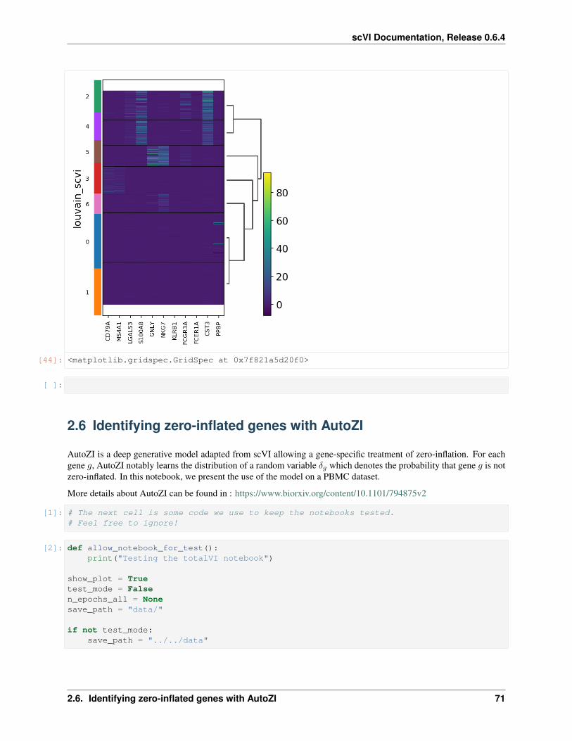
scVI Documentation, Release 0.6.4
[44]: <matplotlib.gridspec.GridSpec at 0x7f821a5d20f0>
[ ]:
2.6 Identifying zero-inflated genes with AutoZI
AutoZI is a deep generative model adapted from scVI allowing a gene-specific treatment of zero-inflation. For eachgene 𝑔, AutoZI notably learns the distribution of a random variable 𝛿𝑔 which denotes the probability that gene 𝑔 is notzero-inflated. In this notebook, we present the use of the model on a PBMC dataset.
More details about AutoZI can be found in : https://www.biorxiv.org/content/10.1101/794875v2
[1]: # The next cell is some code we use to keep the notebooks tested.# Feel free to ignore!
[2]: def allow_notebook_for_test():print("Testing the totalVI notebook")
show_plot = Truetest_mode = Falsen_epochs_all = Nonesave_path = "data/"
if not test_mode:save_path = "../../data"
2.6. Identifying zero-inflated genes with AutoZI 71

scVI Documentation, Release 0.6.4
2.6.1 Imports and data loading
[3]: import matplotlib.pyplot as pltimport numpy as npimport pandas as pdimport torchimport anndataimport os
from scvi.dataset import PbmcDatasetfrom scvi.models import AutoZIVAEfrom scvi.inference import UnsupervisedTrainer
[2019-10-12 22:20:45,665] INFO - scvi._settings | Added StreamHandler with custom→˓formatter to 'scvi' logger./home/oscar/miniconda3/lib/python3.7/site-packages/scikit_learn-0.19.2-py3.7-linux-→˓x86_64.egg/sklearn/ensemble/weight_boosting.py:29: DeprecationWarning: numpy.core.→˓umath_tests is an internal NumPy module and should not be imported. It will be→˓removed in a future NumPy release.from numpy.core.umath_tests import inner1d
[4]: n_genes_to_keep = 100 if test_mode else 1000pbmc = PbmcDataset(save_path=save_path, save_path_10X=os.path.join(save_path, "10X"))pbmc.subsample_genes(new_n_genes=n_genes_to_keep)
[2019-10-12 22:20:50,348] INFO - scvi.dataset.dataset | File /media/storage/Documents/→˓2. Professionnel/UC Berkeley Internship 2019/scVI-C/data/gene_info_pbmc.csv already→˓downloaded[2019-10-12 22:20:50,349] INFO - scvi.dataset.dataset | File /media/storage/Documents/→˓2. Professionnel/UC Berkeley Internship 2019/scVI-C/data/pbmc_metadata.pickle→˓already downloaded[2019-10-12 22:20:50,388] INFO - scvi.dataset.dataset | File /media/storage/Documents/→˓2. Professionnel/UC Berkeley Internship 2019/scVI-C/data/pbmc8k/filtered_gene_bc_→˓matrices.tar.gz already downloaded[2019-10-12 22:20:50,389] INFO - scvi.dataset.dataset10X | Preprocessing dataset[2019-10-12 22:21:04,249] INFO - scvi.dataset.dataset10X | Finished preprocessing→˓dataset[2019-10-12 22:21:04,334] INFO - scvi.dataset.dataset | Remapping batch_indices to [0,→˓N][2019-10-12 22:21:04,334] INFO - scvi.dataset.dataset | Remapping labels to [0,N][2019-10-12 22:21:04,402] INFO - scvi.dataset.dataset | Computing the library size→˓for the new data[2019-10-12 22:21:04,468] INFO - scvi.dataset.dataset | Downsampled from 8381 to 8381→˓cells[2019-10-12 22:21:04,474] INFO - scvi.dataset.dataset | File /media/storage/Documents/→˓2. Professionnel/UC Berkeley Internship 2019/scVI-C/data/pbmc4k/filtered_gene_bc_→˓matrices.tar.gz already downloaded[2019-10-12 22:21:04,474] INFO - scvi.dataset.dataset10X | Preprocessing dataset[2019-10-12 22:21:11,745] INFO - scvi.dataset.dataset10X | Finished preprocessing→˓dataset[2019-10-12 22:21:11,793] INFO - scvi.dataset.dataset | Remapping batch_indices to [0,→˓N][2019-10-12 22:21:11,794] INFO - scvi.dataset.dataset | Remapping labels to [0,N][2019-10-12 22:21:11,823] INFO - scvi.dataset.dataset | Computing the library size→˓for the new data[2019-10-12 22:21:11,855] INFO - scvi.dataset.dataset | Downsampled from 4340 to 4340→˓cells[2019-10-12 22:21:11,902] INFO - scvi.dataset.dataset | Keeping 33694 genes
(continues on next page)
72 Chapter 2. Tutorials
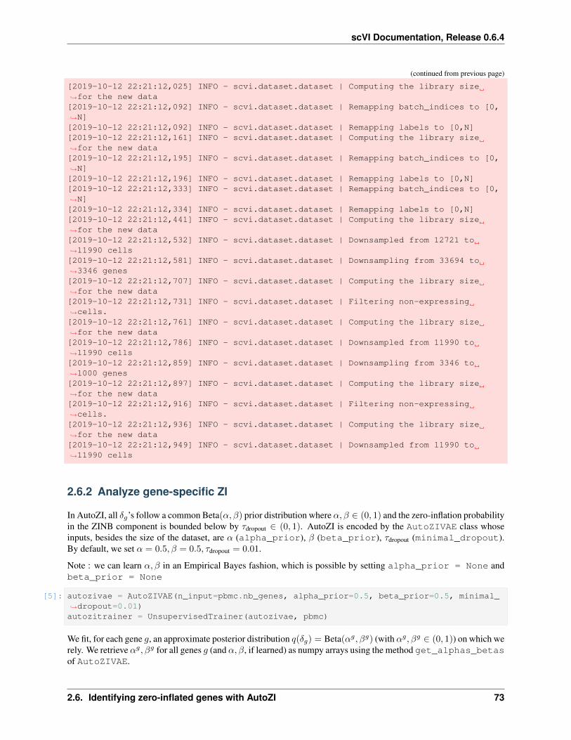
scVI Documentation, Release 0.6.4
(continued from previous page)
[2019-10-12 22:21:12,025] INFO - scvi.dataset.dataset | Computing the library size→˓for the new data[2019-10-12 22:21:12,092] INFO - scvi.dataset.dataset | Remapping batch_indices to [0,→˓N][2019-10-12 22:21:12,092] INFO - scvi.dataset.dataset | Remapping labels to [0,N][2019-10-12 22:21:12,161] INFO - scvi.dataset.dataset | Computing the library size→˓for the new data[2019-10-12 22:21:12,195] INFO - scvi.dataset.dataset | Remapping batch_indices to [0,→˓N][2019-10-12 22:21:12,196] INFO - scvi.dataset.dataset | Remapping labels to [0,N][2019-10-12 22:21:12,333] INFO - scvi.dataset.dataset | Remapping batch_indices to [0,→˓N][2019-10-12 22:21:12,334] INFO - scvi.dataset.dataset | Remapping labels to [0,N][2019-10-12 22:21:12,441] INFO - scvi.dataset.dataset | Computing the library size→˓for the new data[2019-10-12 22:21:12,532] INFO - scvi.dataset.dataset | Downsampled from 12721 to→˓11990 cells[2019-10-12 22:21:12,581] INFO - scvi.dataset.dataset | Downsampling from 33694 to→˓3346 genes[2019-10-12 22:21:12,707] INFO - scvi.dataset.dataset | Computing the library size→˓for the new data[2019-10-12 22:21:12,731] INFO - scvi.dataset.dataset | Filtering non-expressing→˓cells.[2019-10-12 22:21:12,761] INFO - scvi.dataset.dataset | Computing the library size→˓for the new data[2019-10-12 22:21:12,786] INFO - scvi.dataset.dataset | Downsampled from 11990 to→˓11990 cells[2019-10-12 22:21:12,859] INFO - scvi.dataset.dataset | Downsampling from 3346 to→˓1000 genes[2019-10-12 22:21:12,897] INFO - scvi.dataset.dataset | Computing the library size→˓for the new data[2019-10-12 22:21:12,916] INFO - scvi.dataset.dataset | Filtering non-expressing→˓cells.[2019-10-12 22:21:12,936] INFO - scvi.dataset.dataset | Computing the library size→˓for the new data[2019-10-12 22:21:12,949] INFO - scvi.dataset.dataset | Downsampled from 11990 to→˓11990 cells
2.6.2 Analyze gene-specific ZI
In AutoZI, all 𝛿𝑔’s follow a common Beta(𝛼, 𝛽) prior distribution where 𝛼, 𝛽 ∈ (0, 1) and the zero-inflation probabilityin the ZINB component is bounded below by 𝜏dropout ∈ (0, 1). AutoZI is encoded by the AutoZIVAE class whoseinputs, besides the size of the dataset, are 𝛼 (alpha_prior), 𝛽 (beta_prior), 𝜏dropout (minimal_dropout).By default, we set 𝛼 = 0.5, 𝛽 = 0.5, 𝜏dropout = 0.01.
Note : we can learn 𝛼, 𝛽 in an Empirical Bayes fashion, which is possible by setting alpha_prior = None andbeta_prior = None
[5]: autozivae = AutoZIVAE(n_input=pbmc.nb_genes, alpha_prior=0.5, beta_prior=0.5, minimal_→˓dropout=0.01)autozitrainer = UnsupervisedTrainer(autozivae, pbmc)
We fit, for each gene 𝑔, an approximate posterior distribution 𝑞(𝛿𝑔) = Beta(𝛼𝑔, 𝛽𝑔) (with 𝛼𝑔, 𝛽𝑔 ∈ (0, 1)) on which werely. We retrieve 𝛼𝑔, 𝛽𝑔 for all genes 𝑔 (and 𝛼, 𝛽, if learned) as numpy arrays using the method get_alphas_betasof AutoZIVAE.
2.6. Identifying zero-inflated genes with AutoZI 73

scVI Documentation, Release 0.6.4
[6]: n_epochs = 200 if n_epochs_all is None else n_epochs_allautozitrainer.train(n_epochs=n_epochs, lr=1e-2)
training: 100%|| 200/200 [03:58<00:00, 1.20s/it]
[7]: outputs = autozivae.get_alphas_betas()alpha_posterior = outputs['alpha_posterior']beta_posterior = outputs['beta_posterior']
Now that we obtained fitted 𝛼𝑔, 𝛽𝑔 , different metrics are possible. Bayesian decision theory suggests us the posteriorprobability of the zero-inflation hypothesis 𝑞(𝛿𝑔 < 0.5), but also other metrics such as the mean wrt 𝑞 of 𝛿𝑔 arepossible. We focus on the former. We decide that gene 𝑔 is ZI if and only if 𝑞(𝛿𝑔 < 0.5) is greater than a giventhreshold, say 0.5. We may note that it is equivalent to 𝛼𝑔 < 𝛽𝑔 . From this we can deduce the fraction of predicted ZIgenes in the dataset.
[8]: from scipy.stats import beta
# Threshold (or Kzinb/Knb+Kzinb in paper)threshold = 0.5
# q(delta_g < 0.5) probabilitieszi_probs = beta.cdf(0.5,alpha_posterior,beta_posterior)
# ZI genesis_zi_pred = (zi_probs > threshold)
print('Fraction of predicted ZI genes :', is_zi_pred.mean())
Fraction of predicted ZI genes : 0.856
We noted that predictions were less accurate for genes 𝑔 whose average expressions - or predicted NB means, equiva-lently - were low. Indeed, genes assumed not to be ZI were more often predicted as ZI for such low average expressions.A threshold of 1 proved reasonable to separate genes predicted with more or less accuracy. Hence we may want tofocus on predictions for genes with average expression above 1.
[9]: mask_sufficient_expression = (np.array(pbmc.X.mean(axis=0)) > 1.).reshape(-1)print('Fraction of genes with avg expression > 1 :', mask_sufficient_expression.→˓mean())print('Fraction of predicted ZI genes with avg expression > 1 :', is_zi_pred[mask_→˓sufficient_expression].mean())
Fraction of genes with avg expression > 1 : 0.15Fraction of predicted ZI genes with avg expression > 1 : 0.38
2.6.3 Analyze gene-cell-type-specific ZI
One may argue that zero-inflation should also be treated on the cell-type (or ‘label’) level, in addition to the genelevel. AutoZI can be extended by assuming a random variable 𝛿𝑔𝑐 for each gene 𝑔 and cell type 𝑐 which denotes theprobability that gene 𝑔 is not zero-inflated in cell-type 𝑐. The analysis above can be extended to this new scale.
[10]: # Model definitionautozivae_genelabel = AutoZIVAE(n_input=pbmc.nb_genes, alpha_prior=0.5, beta_prior=0.→˓5, minimal_dropout=0.01,
dispersion='gene-label', zero_inflation='gene-label', n_→˓labels=pbmc.n_labels)autozitrainer_genelabel = UnsupervisedTrainer(autozivae_genelabel, pbmc)
(continues on next page)
74 Chapter 2. Tutorials

scVI Documentation, Release 0.6.4
(continued from previous page)
# Trainingn_epochs = 200 if n_epochs_all is None else n_epochs_allautozitrainer_genelabel.train(n_epochs=n_epochs, lr=1e-2)
# Retrieve posterior distribution parametersoutputs_genelabel = autozivae_genelabel.get_alphas_betas()alpha_posterior_genelabel = outputs_genelabel['alpha_posterior']beta_posterior_genelabel = outputs_genelabel['beta_posterior']
training: 100%|| 200/200 [04:34<00:00, 1.29s/it]
[11]: # q(delta_g < 0.5) probabilitieszi_probs_genelabel = beta.cdf(0.5,alpha_posterior_genelabel,beta_posterior_genelabel)
# ZI gene-cell-typesis_zi_pred_genelabel = (zi_probs_genelabel > threshold)
for ind_cell_type, cell_type in enumerate(pbmc.cell_types):
is_zi_pred_genelabel_here = is_zi_pred_genelabel[:,ind_cell_type]print('Fraction of predicted ZI genes for cell type {} :'.format(cell_type),
is_zi_pred_genelabel_here.mean(),'\n')
Fraction of predicted ZI genes for cell type B cells : 0.636
Fraction of predicted ZI genes for cell type CD14+ Monocytes : 0.619
Fraction of predicted ZI genes for cell type CD4 T cells : 0.711
Fraction of predicted ZI genes for cell type CD8 T cells : 0.582
Fraction of predicted ZI genes for cell type Dendritic Cells : 0.56
Fraction of predicted ZI genes for cell type FCGR3A+ Monocytes : 0.557
Fraction of predicted ZI genes for cell type Megakaryocytes : 0.586
Fraction of predicted ZI genes for cell type NK cells : 0.599
Fraction of predicted ZI genes for cell type Other : 0.65
[12]: # With avg expressions > 1for ind_cell_type, cell_type in enumerate(pbmc.cell_types):
mask_sufficient_expression = (np.array(pbmc.X[pbmc.labels.reshape(-1) == ind_cell_→˓type,:].mean(axis=0)) > 1.).reshape(-1)
print('Fraction of genes with avg expression > 1 for cell type {} :'.format(cell_→˓type),
mask_sufficient_expression.mean())is_zi_pred_genelabel_here = is_zi_pred_genelabel[mask_sufficient_expression,ind_
→˓cell_type]print('Fraction of predicted ZI genes with avg expression > 1 for cell type {} :'.
→˓format(cell_type),is_zi_pred_genelabel_here.mean(), '\n')
2.6. Identifying zero-inflated genes with AutoZI 75

scVI Documentation, Release 0.6.4
Fraction of genes with avg expression > 1 for cell type B cells : 0.089Fraction of predicted ZI genes with avg expression > 1 for cell type B cells : 0.→˓16853932584269662
Fraction of genes with avg expression > 1 for cell type CD14+ Monocytes : 0.169Fraction of predicted ZI genes with avg expression > 1 for cell type CD14+ Monocytes :→˓ 0.22485207100591717
Fraction of genes with avg expression > 1 for cell type CD4 T cells : 0.112Fraction of predicted ZI genes with avg expression > 1 for cell type CD4 T cells : 0.→˓25892857142857145
Fraction of genes with avg expression > 1 for cell type CD8 T cells : 0.126Fraction of predicted ZI genes with avg expression > 1 for cell type CD8 T cells : 0.→˓21428571428571427
Fraction of genes with avg expression > 1 for cell type Dendritic Cells : 0.448Fraction of predicted ZI genes with avg expression > 1 for cell type Dendritic Cells :→˓ 0.359375
Fraction of genes with avg expression > 1 for cell type FCGR3A+ Monocytes : 0.283Fraction of predicted ZI genes with avg expression > 1 for cell type FCGR3A+→˓Monocytes : 0.3003533568904594
Fraction of genes with avg expression > 1 for cell type Megakaryocytes : 0.285Fraction of predicted ZI genes with avg expression > 1 for cell type Megakaryocytes :→˓0.39649122807017545
Fraction of genes with avg expression > 1 for cell type NK cells : 0.153Fraction of predicted ZI genes with avg expression > 1 for cell type NK cells : 0.→˓2549019607843137
Fraction of genes with avg expression > 1 for cell type Other : 0.257Fraction of predicted ZI genes with avg expression > 1 for cell type Other : 0.→˓4085603112840467
[ ]:
2.7 Introduction to gimVI
2.7.1 Impute missing genes in Spatial Data from Sequencing Data
[1]: import sys
sys.path.append("../../")sys.path.append("../")
[2]: def allow_notebook_for_test():print("Testing the gimvi notebook")
test_mode = False(continues on next page)
76 Chapter 2. Tutorials
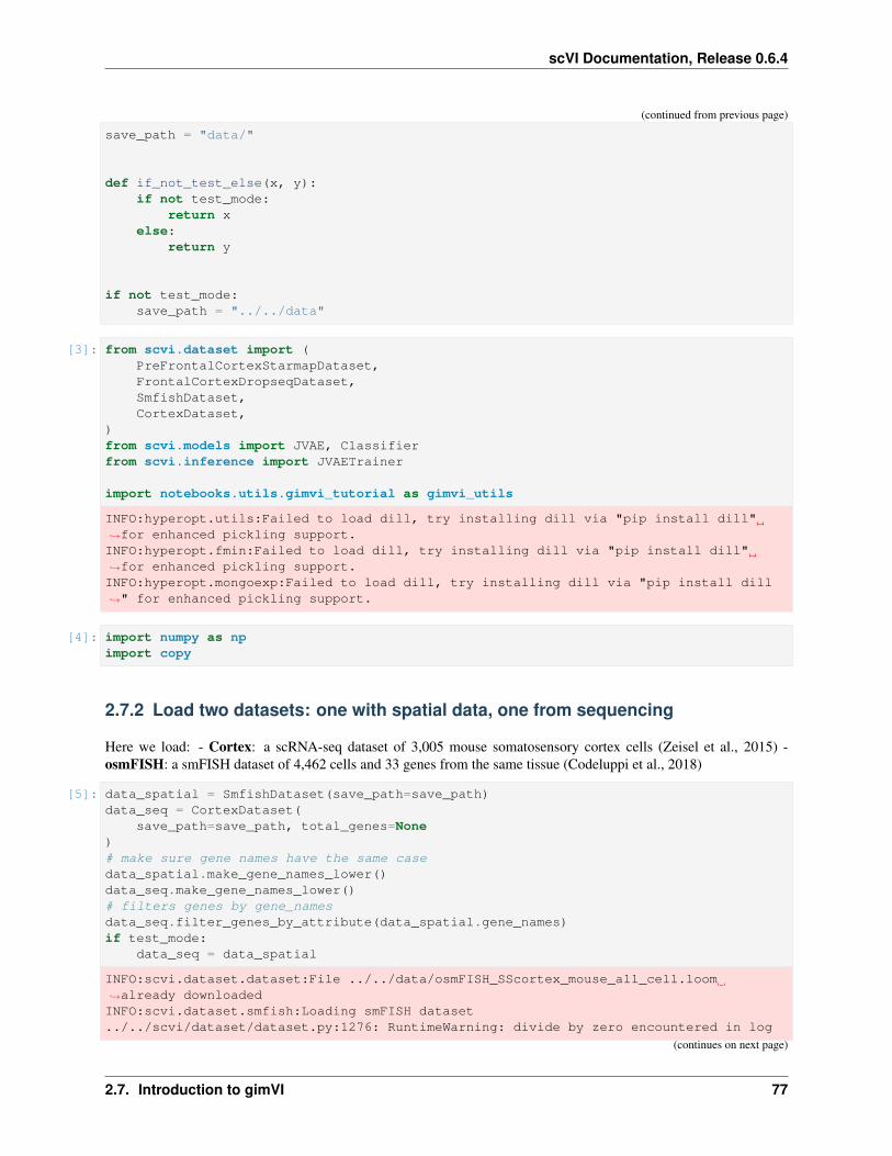
scVI Documentation, Release 0.6.4
(continued from previous page)
save_path = "data/"
def if_not_test_else(x, y):if not test_mode:
return xelse:
return y
if not test_mode:save_path = "../../data"
[3]: from scvi.dataset import (PreFrontalCortexStarmapDataset,FrontalCortexDropseqDataset,SmfishDataset,CortexDataset,
)from scvi.models import JVAE, Classifierfrom scvi.inference import JVAETrainer
import notebooks.utils.gimvi_tutorial as gimvi_utils
INFO:hyperopt.utils:Failed to load dill, try installing dill via "pip install dill"→˓for enhanced pickling support.INFO:hyperopt.fmin:Failed to load dill, try installing dill via "pip install dill"→˓for enhanced pickling support.INFO:hyperopt.mongoexp:Failed to load dill, try installing dill via "pip install dill→˓" for enhanced pickling support.
[4]: import numpy as npimport copy
2.7.2 Load two datasets: one with spatial data, one from sequencing
Here we load: - Cortex: a scRNA-seq dataset of 3,005 mouse somatosensory cortex cells (Zeisel et al., 2015) -osmFISH: a smFISH dataset of 4,462 cells and 33 genes from the same tissue (Codeluppi et al., 2018)
[5]: data_spatial = SmfishDataset(save_path=save_path)data_seq = CortexDataset(
save_path=save_path, total_genes=None)# make sure gene names have the same casedata_spatial.make_gene_names_lower()data_seq.make_gene_names_lower()# filters genes by gene_namesdata_seq.filter_genes_by_attribute(data_spatial.gene_names)if test_mode:
data_seq = data_spatial
INFO:scvi.dataset.dataset:File ../../data/osmFISH_SScortex_mouse_all_cell.loom→˓already downloadedINFO:scvi.dataset.smfish:Loading smFISH dataset../../scvi/dataset/dataset.py:1276: RuntimeWarning: divide by zero encountered in log
(continues on next page)
2.7. Introduction to gimVI 77

scVI Documentation, Release 0.6.4
(continued from previous page)
log_counts = np.log(data.sum(axis=1))/home/achille/miniconda3/envs/scvi-update/lib/python3.7/site-packages/numpy/core/_→˓methods.py:117: RuntimeWarning: invalid value encountered in subtractx = asanyarray(arr - arrmean)
INFO:scvi.dataset.dataset:Computing the library size for the new dataINFO:scvi.dataset.dataset:Downsampled from 6471 to 4530 cellsINFO:scvi.dataset.dataset:Remapping labels to [0,N]INFO:scvi.dataset.dataset:Remapping batch_indices to [0,N]INFO:scvi.dataset.dataset:File ../../data/expression.bin already downloadedINFO:scvi.dataset.cortex:Loading Cortex dataINFO:scvi.dataset.cortex:Finished preprocessing Cortex dataINFO:scvi.dataset.dataset:Remapping labels to [0,N]INFO:scvi.dataset.dataset:Remapping batch_indices to [0,N]
• FrontalCortexDropseq: a scRNA-seq dataset of 71,639 mouse frontal cortex cells (Saunders et al., 2018)
• PreFrontalCortexStarmap: a starMAP dataset of 3,704 cells and 166 genes from the mouse pre-frontal cortex(Wang et al., 2018)
[6]: # data_spatial = PreFrontalCortexStarmapDataset(save_path=save_path)# data_seq = FrontalCortexDropseqDataset(# save_path=save_path, genes_to_keep=data_spatial.gene_names# )# data_seq.subsample_cells(5000)
Hide some genes in the osFISH dataset to score the imputation
[7]: data_seq.filter_cells_by_count(1)data_spatial.filter_cells_by_count(1)
INFO:scvi.dataset.dataset:Computing the library size for the new dataINFO:scvi.dataset.dataset:Downsampled from 3005 to 2996 cellsINFO:scvi.dataset.dataset:Computing the library size for the new dataINFO:scvi.dataset.dataset:Downsampled from 4530 to 4530 cells
[8]: train_size = 0.8
gene_names_rnaseq = data_seq.gene_namesnp.random.seed(0)n_genes = len(gene_names_rnaseq)gene_ids_train = sorted(
np.random.choice(range(n_genes), int(n_genes * train_size), False))gene_ids_test = sorted(set(range(n_genes)) - set(gene_ids_train))
gene_names_fish = gene_names_rnaseq[gene_ids_train]
# Create copy of the fish dataset with hidden genesdata_spatial_partial = copy.deepcopy(data_spatial)data_spatial_partial.filter_genes_by_attribute(gene_names_fish)data_spatial_partial.batch_indices += data_seq.n_batches
INFO:scvi.dataset.dataset:Downsampling from 33 to 26 genesINFO:scvi.dataset.dataset:Computing the library size for the new dataINFO:scvi.dataset.dataset:Filtering non-expressing cells.INFO:scvi.dataset.dataset:Computing the library size for the new dataINFO:scvi.dataset.dataset:Downsampled from 4530 to 4530 cells
78 Chapter 2. Tutorials

scVI Documentation, Release 0.6.4
Configure the Joint Model The joint model can take multiple datasets with potentially different observed genes. Alldataset will be encoded and decoded with the union of all genes. It requires: - The gene mappings from each datasetto the common decoded vector: * Eg: dataset1 has genes [‘a’, ‘b’] and dataset2 has genes [‘b’, ‘c’], then a possibleoutput can be [‘b’, ‘a’, ‘c’] such that the mappings are [1, 0] and [0, 2] * Usually, if the genes of dataset2 are includedin dataset1, it is way more efficient to keep the order of dataset1 in the output and use ``slice(None)`` as a mappingfor dataset1
• The number of inputs (ie) number of genes in each dataset
• The distributions to use for the generative process: usually scRNA-seq is modelled with ZINB (because oftechnical dropout) and FISH with NB or even Poisson
• Whether to model the library size with a latent variable or use the observed value
[9]: datasets = [data_seq, data_spatial_partial]generative_distributions = ["zinb", "nb"]gene_mappings = [slice(None), np.array(gene_ids_train)]n_inputs = [d.nb_genes for d in datasets]total_genes = data_seq.nb_genesn_batches = sum([d.n_batches for d in datasets])
model_library_size = [True, False]
n_latent = 8kappa = 1
[10]: import torch
torch.manual_seed(0)
model = JVAE(n_inputs,total_genes,gene_mappings,generative_distributions,model_library_size,n_layers_decoder_individual=0,n_layers_decoder_shared=0,n_layers_encoder_individual=1,n_layers_encoder_shared=1,dim_hidden_encoder=64,dim_hidden_decoder_shared=64,dropout_rate_encoder=0.2,dropout_rate_decoder=0.2,n_batch=n_batches,n_latent=n_latent,
)
discriminator = Classifier(n_latent, 32, 2, 3, logits=True)
trainer = JVAETrainer(model, discriminator, datasets, 0.95, frequency=1, kappa=kappa)
[11]: n_epochs = if_not_test_else(200, 1)trainer.train(n_epochs=n_epochs)
training: 100%|| 200/200 [04:24<00:00, 1.27s/it]
2.7. Introduction to gimVI 79

scVI Documentation, Release 0.6.4
[12]: gimvi_utils.plot_umap(trainer)
[13]: gimvi_utils.imputation_score(trainer, data_spatial, gene_ids_test, True)
[13]: 0.25089044336342275
Plot imputation for LAMP5, hidden in the training
[14]: gimvi_utils.plot_gene_spatial(trainer, data_spatial, 9)
80 Chapter 2. Tutorials

scVI Documentation, Release 0.6.4
Inspect classification accuracy (we expect a uniform matrix)
If the matrix is diagonal, the kappa needs to be scaled up to ensure mixing.
[15]: discriminator_classification = trainer.get_discriminator_confusion()discriminator_classification
[15]: array([[0.5616336 , 0.43836704],[0.41276518, 0.58723474]], dtype=float32)
[16]: import pandas as pd
results = pd.DataFrame(trainer.get_loss_magnitude(),index=["reconstruction", "kl_divergence", "discriminator"],columns=["Sequencing", "Spatial"],
)results.columns.name = "Dataset"results.index.name = "Loss"results
[16]: Dataset Sequencing SpatialLossreconstruction 868.178913 1765.545235kl_divergence 201.512057 206.783453discriminator 24.937387 20.623563
2.8 Linearly decoded VAE
This notebook shows how to use the ‘linearly decoded VAE’ model which explicitly links latent variables of cells togenes.
The scVI package learns low-dimensional latent representations of cells which get mapped to parameters of probabilitydistributions which can generate counts consistent to what is observed from data. In the standard VAE model of scVIthese parameters for each gene and cell arise from applying neural networks to the latent variables. Neural networksare flexible and can represent non-linearities in the data. This comes at a price, there is no direct link between a latentvariable dimension and any potential set of genes which would covary across it.
The LDVAE model replaces the neural networks with linear functions. Now a higher value along a latent dimensionwill directly correspond to higher expression of the genes with high weights assigned to that dimension.
This leads to a generative model comparable to probabilistic PCA or factor analysis, but generates counts rather thanreal numbers. Using the framework of scVI also allows variational inference which scales to very large datasets andcan make use of GPUs for additional speed.
This notebook demonstrates how to fit an LDVAE model to scRNA-seq data, plot the latent variables, and interpretwhich genes are linked to latent variables.
As an example, we use the PBMC 10K from 10x Genomics.
[1]: # Cell left blank for testing purposes
Automated testing configuration
[2]: import os
def allow_notebook_for_test():
(continues on next page)
2.8. Linearly decoded VAE 81

scVI Documentation, Release 0.6.4
(continued from previous page)
print("Testing the ldvae notebook")
test_mode = Falsesave_path = "data/"n_epochs_all = Noneshow_plot = True
if not test_mode:save_path = "../../data"
data_path = os.path.join(save_path, "filtered_gene_bc_matrices/hg19/")
[3]: import torch
from scvi.dataset import GeneExpressionDataset, Dataset10Xfrom scvi.models import LDVAEfrom scvi.inference import UnsupervisedTrainer, Trainerfrom scvi.inference.posterior import Posterior
import pandas as pdimport anndataimport scanpy as sc
import matplotlib.pyplot as plt
if not test_mode:%matplotlib inline
[2019-11-08 08:29:48,883] INFO - scvi._settings | Added StreamHandler with custom→˓formatter to 'scvi' logger./data/yosef2/users/adamgayoso/.pyenv/versions/scvi/lib/python3.7/site-packages/→˓sklearn/utils/linear_assignment_.py:21: DeprecationWarning: The linear_assignment_→˓module is deprecated in 0.21 and will be removed from 0.23. Use scipy.optimize.→˓linear_sum_assignment instead.DeprecationWarning)
2.8.1 Initialization
[4]: import torchimport numpy as npfrom scvi import set_seed
# Setting seeds for reproducibilityset_seed(0)
[5]: cells_dataset = Dataset10X(dataset_name="pbmc_10k_protein_v3",save_path=os.path.join(save_path, "10X"),measurement_names_column=1,dense=True,
)
82 Chapter 2. Tutorials
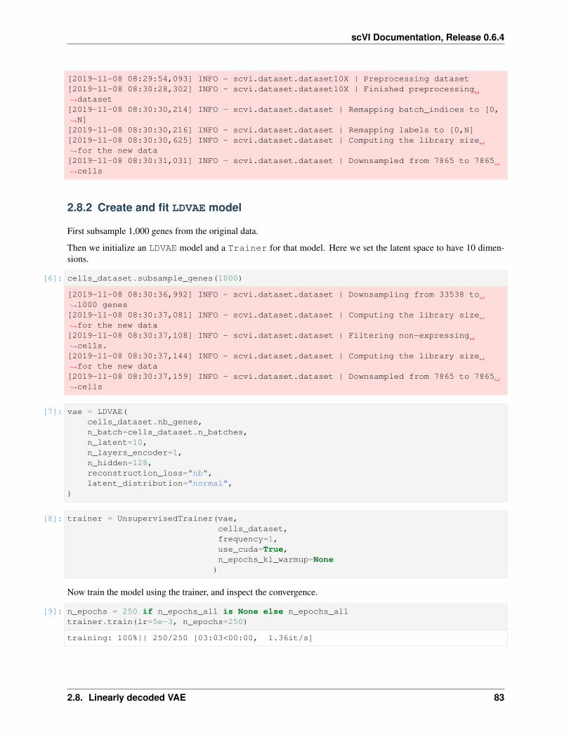
scVI Documentation, Release 0.6.4
[2019-11-08 08:29:54,093] INFO - scvi.dataset.dataset10X | Preprocessing dataset[2019-11-08 08:30:28,302] INFO - scvi.dataset.dataset10X | Finished preprocessing→˓dataset[2019-11-08 08:30:30,214] INFO - scvi.dataset.dataset | Remapping batch_indices to [0,→˓N][2019-11-08 08:30:30,216] INFO - scvi.dataset.dataset | Remapping labels to [0,N][2019-11-08 08:30:30,625] INFO - scvi.dataset.dataset | Computing the library size→˓for the new data[2019-11-08 08:30:31,031] INFO - scvi.dataset.dataset | Downsampled from 7865 to 7865→˓cells
2.8.2 Create and fit LDVAE model
First subsample 1,000 genes from the original data.
Then we initialize an LDVAE model and a Trainer for that model. Here we set the latent space to have 10 dimen-sions.
[6]: cells_dataset.subsample_genes(1000)
[2019-11-08 08:30:36,992] INFO - scvi.dataset.dataset | Downsampling from 33538 to→˓1000 genes[2019-11-08 08:30:37,081] INFO - scvi.dataset.dataset | Computing the library size→˓for the new data[2019-11-08 08:30:37,108] INFO - scvi.dataset.dataset | Filtering non-expressing→˓cells.[2019-11-08 08:30:37,144] INFO - scvi.dataset.dataset | Computing the library size→˓for the new data[2019-11-08 08:30:37,159] INFO - scvi.dataset.dataset | Downsampled from 7865 to 7865→˓cells
[7]: vae = LDVAE(cells_dataset.nb_genes,n_batch=cells_dataset.n_batches,n_latent=10,n_layers_encoder=1,n_hidden=128,reconstruction_loss="nb",latent_distribution="normal",
)
[8]: trainer = UnsupervisedTrainer(vae,cells_dataset,frequency=1,use_cuda=True,n_epochs_kl_warmup=None
)
Now train the model using the trainer, and inspect the convergence.
[9]: n_epochs = 250 if n_epochs_all is None else n_epochs_alltrainer.train(lr=5e-3, n_epochs=250)
training: 100%|| 250/250 [03:03<00:00, 1.36it/s]
2.8. Linearly decoded VAE 83

scVI Documentation, Release 0.6.4
[10]: if not test_mode:fig, ax = plt.subplots(figsize=(6, 4))ax.plot(trainer.history['elbo_train_set'][10:])ax.plot(trainer.history['elbo_test_set'][10:])
2.8.3 Extract and plot latent dimensions for cells
From the fitted model we extract the (mean) values for the latent dimensions. We store the values in the AnnDataobject for convenience.
[11]: full = trainer.create_posterior(trainer.model, cells_dataset, indices=np.→˓arange(len(cells_dataset)))Z_hat = full.sequential().get_latent()[0]adata = anndata.AnnData(cells_dataset.X)
[12]: for i, z in enumerate(Z_hat.T):adata.obs[f'Z_{i}'] = z
Now we can plot the latent dimension coordinates for each cell. A quick (albeit not complete) way to view these is tomake a series of 2D scatter plots that cover all the dimensions. Since we are representing the cells by 10 dimensions,this leads to 5 scatter plots.
[13]: fig = plt.figure(figsize=(12, 8))
for f in range(0, 9, 2):plt.subplot(2, 3, int(f / 2) + 1)
plt.scatter(adata.obs[f'Z_{f}'], adata.obs[f'Z_{f + 1}'], marker='.', s=4, label=→˓'Cells')
plt.xlabel(f'Z_{f}')plt.ylabel(f'Z_{f + 1}')
plt.subplot(2, 3, 6)plt.scatter(adata.obs[f'Z_{f}'], adata.obs[f'Z_{f + 1}'], marker='.', label='Cells',→˓s=4)plt.scatter(adata.obs[f'Z_{f}'], adata.obs[f'Z_{f + 1}'], c='w', label=None)
(continues on next page)
84 Chapter 2. Tutorials
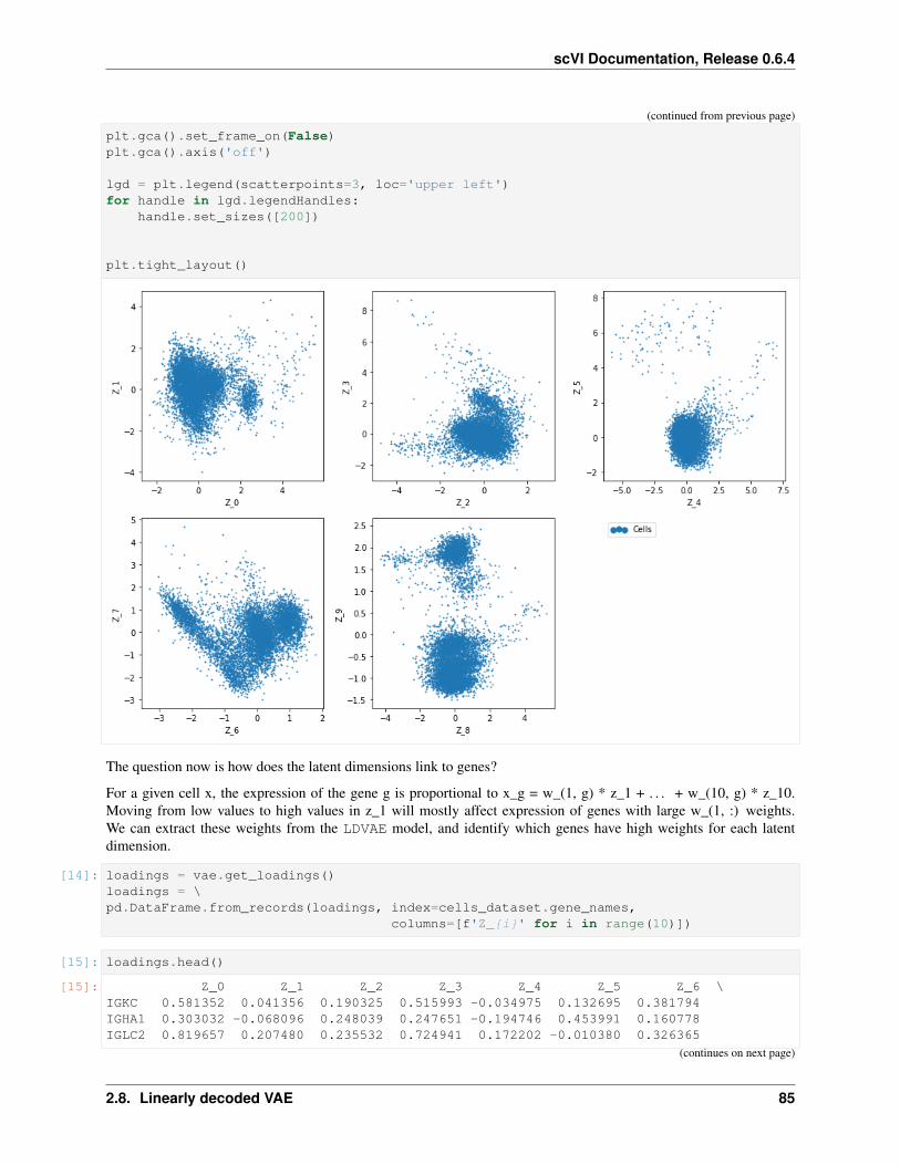
scVI Documentation, Release 0.6.4
(continued from previous page)
plt.gca().set_frame_on(False)plt.gca().axis('off')
lgd = plt.legend(scatterpoints=3, loc='upper left')for handle in lgd.legendHandles:
handle.set_sizes([200])
plt.tight_layout()
The question now is how does the latent dimensions link to genes?
For a given cell x, the expression of the gene g is proportional to x_g = w_(1, g) * z_1 + . . . + w_(10, g) * z_10.Moving from low values to high values in z_1 will mostly affect expression of genes with large w_(1, :) weights.We can extract these weights from the LDVAE model, and identify which genes have high weights for each latentdimension.
[14]: loadings = vae.get_loadings()loadings = \pd.DataFrame.from_records(loadings, index=cells_dataset.gene_names,
columns=[f'Z_{i}' for i in range(10)])
[15]: loadings.head()
[15]: Z_0 Z_1 Z_2 Z_3 Z_4 Z_5 Z_6 \IGKC 0.581352 0.041356 0.190325 0.515993 -0.034975 0.132695 0.381794IGHA1 0.303032 -0.068096 0.248039 0.247651 -0.194746 0.453991 0.160778IGLC2 0.819657 0.207480 0.235532 0.724941 0.172202 -0.010380 0.326365
(continues on next page)
2.8. Linearly decoded VAE 85

scVI Documentation, Release 0.6.4
(continued from previous page)
IGLC3 0.818061 0.455800 0.132923 0.660388 -0.087060 -0.093394 0.389668IGHM 0.874641 0.312170 0.287022 0.963226 0.108258 -0.034833 0.627738
Z_7 Z_8 Z_9IGKC 0.088605 0.078768 -0.323640IGHA1 0.013388 0.090267 -0.266768IGLC2 -0.420546 0.433572 -0.171949IGLC3 -0.168332 0.151087 -0.291709IGHM 0.031824 0.096756 -0.368698
For every latent variable Z, we extract the genes with largest magnitude, and separate genes with large negative valuesfrom genes with large positive values. We print out the top 5 genes in each direction for each latent variable.
[16]: print('Top loadings by magnitude\n---------------------')for clmn_ in loadings:
loading_ = loadings[clmn_].sort_values()fstr = clmn_ + ':\t'fstr += '\t'.join([f'{i}, {loading_[i]:.2}' for i in loading_.head(5).index])fstr += '\n\t...\n\t'fstr += '\t'.join([f'{i}, {loading_[i]:.2}' for i in loading_.tail(5).index])print(fstr + '\n---------------------\n')
Top loadings by magnitude---------------------Z_0: S100A12, -1.1 IL7R, -0.89 VCAN, -0.89 S100A8, -0.86 G0S2, -0.85
...CD79A, 0.98 HLA-DQB1, 1.0 IGLL5, 1.1 HLA-DQA2, 1.1 HLA-DQA1, 1.3
---------------------
Z_1: ITGB1, -0.44 HBB, -0.37 KLF6, -0.29 LTB, -0.29 CORO1B, -0.26...FGFBP2, 0.69 TRDC, 0.72 KLRF1, 0.73 PTGDS, 0.86 GZMB, 0.91
---------------------
Z_2: C1QB, -1.0 LYPD2, -0.96 C1QA, -0.93 CDKN1C, -0.84 UBE2C, -0.55...DERL3, 0.35 ALOX5AP, 0.38 GZMB, 0.42 PTGDS, 0.52 IGHG2, 0.62
---------------------
Z_3: FCER1A, -0.72 CLEC10A, -0.5 S100A12, -0.49 C1QB, -0.47 PLBD1, -0.46...IGHG2, 0.92 IGHM, 0.96 MS4A1, 1.0 IGHD, 1.2 TCL1A, 1.2
---------------------
Z_4: KLRF1, -0.4 XBP1, -0.34 TYROBP, -0.33 MYDGF, -0.32 GNLY, -0.3...FCER1A, 0.45 GZMK, 0.66 PCLAF, 0.66 CD8B, 0.67 PPBP, 0.79
---------------------
Z_5: TCL1A, -0.97 C1QA, -0.94 FCGR3A, -0.87 IGHD, -0.85 C1QB, -0.77...PCLAF, 0.46 TYMS, 0.46 TNFRSF17, 0.51 IGHA2, 0.53 AQP3, 0.59
---------------------
Z_6: GNLY, -1.9 GZMH, -1.9 NKG7, -1.9 CCL5, -1.8 GZMA, -1.8...VCAN, 0.74 AIF1, 0.74 LGALS2, 0.76 KCTD12, 0.77 IGLC7, 0.79
(continues on next page)
86 Chapter 2. Tutorials

scVI Documentation, Release 0.6.4
(continued from previous page)
---------------------
Z_7: GZMK, -1.4 CLEC10A, -1.2 KLRB1, -0.95 FCER1A, -0.73 CCL5, -0.69...PPBP, 0.45 RRM2, 0.54 HBA2, 0.59 IGHG2, 1.4 HBB, 1.5
---------------------
Z_8: LYPD2, -1.1 C1QA, -0.76 CDKN1C, -0.76 C1QB, -0.69 FCGR3A, -0.59...UBE2C, 0.45 ITM2C, 0.51 TCL1A, 0.53 DERL3, 0.61 GZMK, 0.61
---------------------
Z_9: CD8B, -2.2 GZMK, -1.9 TRAC, -1.7 CD3G, -1.7 CD3D, -1.6...CST3, 1.7 S100A12, 1.7 S100A8, 1.9 S100A9, 1.9 LYZ, 1.9
---------------------
It is important to keep in mind that unlike traditional PCA, these latent variables are not ordered. Z_0 does notnecessarily explain more variance than Z_1.
These top genes can be interpreted as following most of the structural variation in the data.
The LDVAE model further supports the same scVI functionality as the VAE model, so all posterior methods work thesame. Here we show how to use scanpy to visualize the latent space.
[17]: adata.obsm["X_scVI"] = Z_hatsc.pp.neighbors(adata, use_rep="X_scVI", n_neighbors=20)sc.tl.umap(adata, min_dist=0.1)sc.tl.leiden(adata, key_added="leiden_scVI", resolution=0.8)
[18]: sc.pl.umap(adata, color=["leiden_scVI"], show=show_plot)
[19]: zs = [f'Z_{i}' for i in range(vae.n_latent)]sc.pl.umap(adata, color=zs, show=show_plot, ncols=3)
2.8. Linearly decoded VAE 87

scVI Documentation, Release 0.6.4
2.9 Advanced autotune tutorial
DISCLAIMER: Most experiments in this notebook require one or more GPUs to keep their runtime a matterof hours. DISCLAIMER: To use our new autotune feature in parallel mode, you need to install `MongoDb<https://docs.mongodb.com/manual/installation/>`__ first.
In this notebook, we give an in-depth tutorial on scVI’s new autotune module.
Overall, the new module enables users to perform parallel hyperparemter search for any scVI model and on any numberof GPUs/CPUs. Although, the search may be performed sequentially using only one GPU/CPU, we will focus on theparalel case. Note that GPUs provide a much faster approach as they are particularly suitable for neural networksgradient back-propagation.
Additionally, we provide the code used to generate the results presented in our Hyperoptimization blog post. For anin-depth analysis of the results obtained on three gold standard scRNAseq datasets (Cortex, PBMC and BrainLarge),please to the above blog post. In the blog post, we also suggest guidelines on how and when to use our auto-tuningfeature.
88 Chapter 2. Tutorials

scVI Documentation, Release 0.6.4
[1]: import sys
sys.path.append("../../")sys.path.append("../")
%matplotlib inline
/home/ec2-user
[2]: import loggingimport osimport pickle
import matplotlib.pyplot as pltimport numpy as npimport pandas as pdimport torchfrom hyperopt import hp
from scvi.dataset import BrainLargeDataset, CortexDataset, LoomDataset, PbmcDatasetfrom scvi.inference import UnsupervisedTrainerfrom scvi.inference.autotune import auto_tune_scvi_modelfrom scvi.models import VAE
[ ]: logger = logging.getLogger("scvi.inference.autotune")logger.setLevel(logging.WARNING)
[2]: def allow_notebook_for_test():print("Testing the autotune advanced notebook")
test_mode = False
def if_not_test_else(x, y):if not test_mode:
return xelse:
return y
save_path = "data/"n_epochs = if_not_test_else(1000, 1)n_epochs_brain_large = if_not_test_else(50, 1)max_evals = if_not_test_else(100, 1)reserve_timeout = if_not_test_else(180, 5)fmin_timeout = if_not_test_else(300, 10)
2.9. Advanced autotune tutorial 89

scVI Documentation, Release 0.6.4
2.9.1 Default usage
For the sake of principled simplicity, we provide an all-default approach to hyperparameter search for any scVImodel. The few lines below present an example of how to perform hyper-parameter search for scVI on the Cortexdataset.
Note that, by default, the model used is scVI’s VAE and the trainer is the UnsupervisedTrainer
Also, the default search space is as follows: * n_latent: [5, 15] * n_hidden: {64, 128, 256} * n_layers: [1,5] * dropout_rate: {0.1, 0.3, 0.5, 0.7} * reconstruction_loss: {“zinb”, “nb”} * lr: {0.01, 0.005, 0.001,0.0005, 0.0001}
On a more practical note, verbosity varies in the following way: * logger.setLevel(logging.WARNING)will show a progress bar. * logger.setLevel(logging.INFO) will show global logs including the number ofjobs done. * logger.setLevel(logging.DEBUG) will show detailed logs for each training (e.g the parameterstested).
This function’s behaviour can be customized, please refer to the rest of this tutorial as well as its documentation forinformation about the different parameters available.
Running the hyperoptimization process.
[ ]: cortex_dataset = CortexDataset(save_path=save_path)
INFO:scvi.dataset.dataset:File tests/data/expression.bin already downloadedINFO:scvi.dataset.cortex:Loading Cortex data
[5]: best_trainer, trials = auto_tune_scvi_model(gene_dataset=cortex_dataset,parallel=True,exp_key="cortex_dataset",train_func_specific_kwargs={"n_epochs": n_epochs},max_evals=max_evals,reserve_timeout=reserve_timeout,fmin_timeout=fmin_timeout,
)
100%|| 100/100 [3:21:15<00:00, 102.45s/it]
Returned objects
The trials object contains detailed information about each run. trials.trials is an Iterable in whicheach element corresponds to a single run. It can be used as a dictionary for wich the key “result” yields a dictionnarycontaining the outcome of the run as defined in our default objective function (or the user’s custom version). Forexample, it will contain information on the hyperparameters used (under the “space” key), the resulting metric (underthe “loss” key) or the status of the run.
The best_trainer object can be used directly as an scVI Trainer object. It is the result of a training on thewhole dataset provided using the optimal set of hyperparameters found.
90 Chapter 2. Tutorials

scVI Documentation, Release 0.6.4
2.9.2 Custom hyperamater space
Although our default can be a good one in a number of cases, we still provide an easy way to use custom values forthe hyperparameters search space. These are broken down in three categories: * Hyperparameters for the Trainerinstance. (if any) * Hyperparameters for the Trainer instance’s train method. (e.g lr) * Hyperparameters forthe model instance. (e.g n_layers)
To build your own hyperparameter space follow the scheme used in scVI’s codebase as well as the sample below.Note the various spaces you define, have to follow the hyperopt syntax, for which you can find a detailed descriptionhere.
For example, if you were to want to search over a continuous range of droupouts varying in [0.1, 0.3] and for acontinuous learning rate varying in [0.001, 0.0001], you could use the following search space.
[ ]: space = {"model_tunable_kwargs": {"dropout_rate": hp.uniform("dropout_rate", 0.1, 0.3)},"train_func_tunable_kwargs": {"lr": hp.loguniform("lr", -4.0, -3.0)},
}
best_trainer, trials = auto_tune_scvi_model(gene_dataset=cortex_dataset,space=space,parallel=True,exp_key="cortex_dataset_custom_space",train_func_specific_kwargs={"n_epochs": n_epochs},max_evals=max_evals,reserve_timeout=reserve_timeout,fmin_timeout=fmin_timeout,
)
2.9.3 Custom objective metric
By default, our autotune process tracks the marginal negative log likelihood of the best state of the model according otthe held-out Evidence Lower BOund (ELBO). But, if you want to track a different early stopping metric and optimizea different loss you can use auto_tune_scvi_model’s parameters.
For example, if for some reason, you had a dataset coming from two batches (i.e two merged datasets) and wantedto optimize the hyperparameters for the batch mixing entropy. You could use the code below, which makes use ofthe metric_name argument of auto_tune_scvi_model. This can work for any metric that is implemented inthe Posterior class you use. You may also specify the name of the Posterior attribute you want to use (e.g“train_set”).
[ ]: pbmc_dataset = PbmcDataset(save_path=save_path, save_path_10X=os.path.join(save_path, "10X")
)
[ ]: best_trainer, trials = auto_tune_scvi_model(gene_dataset=pbmc_dataset,metric_name="entropy_batch_mixing",posterior_name="train_set",parallel=True,exp_key="pbmc_entropy_batch_mixing",train_func_specific_kwargs={"n_epochs": n_epochs},max_evals=max_evals,reserve_timeout=reserve_timeout,
(continues on next page)
2.9. Advanced autotune tutorial 91

scVI Documentation, Release 0.6.4
(continued from previous page)
fmin_timeout=fmin_timeout,)
2.9.4 Custom objective function
Below, we describe, using one of our Synthetic dataset, how to tune our annotation model SCANVI for, e.g, betteraccuracy on a 20% subset of the labelled data. Note that the model is trained in a semi-supervised framework, that iswhy we have a labelled and unlabelled dataset. Please, refer to the original paper for details on SCANVI!
In this case, as described in our annotation notebook we may want to form the labelled/unlabelled sets usingbatch indices. Unfortunately, that requires a little “by hand” work. Even in that case, we are able to leverage the newautotune module to perform hyperparameter tuning. In order to do so, one has to write his own objective function andfeed it to auto_tune_scvi_model.
One can proceed as described below. Note three important conditions: * Since it is going to be pickled the objectiveshould not be implemented in the “main” module, i.e an executable script or a notebook. * the objective should havethe search space as its first attribute and a boolean is_best_training as its second. * If not using a cutstom searchspace, it should be expected to take the form of a dictionary with the following keys: * "model_tunable_kwargs" * "trainer_tunable_kwargs" * "train_func_tunable_kwargs"
[ ]: synthetic_dataset = LoomDataset(filename="simulation_1.loom",save_path=os.path.join(save_path, "simulation/"),url="https://github.com/YosefLab/scVI-data/raw/master/simulation/simulation_1.loom
→˓",)
[ ]: from notebooks.utils.autotune_advanced_notebook import custom_objective_hyperopt
[ ]: objective_kwargs = dict(dataset=synthetic_dataset, n_epochs=n_epochs)best_trainer, trials = auto_tune_scvi_model(
custom_objective_hyperopt=custom_objective_hyperopt,objective_kwargs=objective_kwargs,parallel=True,exp_key="synthetic_dataset_scanvi",max_evals=max_evals,reserve_timeout=reserve_timeout,fmin_timeout=fmin_timeout,
)
2.9.5 Delayed populating, for very large datasets.
DISCLAIMER: We don’t actually need this for the BrainLarge dataset with 720 genes, this is just an example.
The fact is that after building the objective function and feeding it to hyperopt, it is pickled on to theMongoWorkers. Thus, if you pass a loaded dataset as a partial argument to the objective function, and this datasetexceeds 4Gb, you’ll get a PickleError (Objects larger than 4Gb can’t be pickled).
To remedy this issue, in case you have a very large dataset for which you want to perform hyperparameter optimization,you should subclass scVI’s DownloadableDataset or use one of its many existing subclasses, such that thedataset can be populated inside the objective function which is called by each worker.
92 Chapter 2. Tutorials

scVI Documentation, Release 0.6.4
[ ]: brain_large_dataset = BrainLargeDataset(save_path=save_path, delayed_populating=True)best_trainer, trials = auto_tune_scvi_model(
gene_dataset=brain_large_dataset,delayed_populating=True,parallel=True,exp_key="brain_large_dataset",max_evals=max_evals,trainer_specific_kwargs={
"early_stopping_kwargs": {"early_stopping_metric": "elbo","save_best_state_metric": "elbo","patience": 20,"threshold": 0,"reduce_lr_on_plateau": True,"lr_patience": 10,"lr_factor": 0.2,
}},train_func_specific_kwargs={"n_epochs": n_epochs_brain_large},reserve_timeout=reserve_timeout,fmin_timeout=fmin_timeout,
)
2.9.6 Blog post reproducibility
Below, we provide some code to reproduce the results of our blog post on hyperparameter search with scVI. Note, thatthis can also be used as a tutorial on how to make senss of the output of the autotuning process, the Trials object.
2.9.7 Cortex, Pbmc and BrainLarge hyperparameter optimization
First off, we run the default hyperparameter optimization procedure (default search space, 100 runs) on each of thethree dataset of our study: * The Cortex dataset (done above) * The Pbmc dataset * The Brain Large dataset (doneabove)
[ ]: best_trainer, trials = auto_tune_scvi_model(gene_dataset=pbmc_dataset,parallel=True,exp_key="pbmc_dataset",max_evals=max_evals,train_func_specific_kwargs={"n_epochs": n_epochs},reserve_timeout=reserve_timeout,fmin_timeout=fmin_timeout,
)
INFO:scvi.inference.autotune:Starting experiment: pbmc_bisDEBUG:scvi.inference.autotune:Using default parameter search space.INFO:scvi.inference.autotune:Fixed parameters:model:{}trainer:{'early_stopping_kwargs': {'early_stopping_metric': 'll', 'save_best_state_metric':→˓'ll', 'patience': 50, 'threshold': 0, 'reduce_lr_on_plateau': False, 'lr_patience':→˓25, 'lr_factor': 0.2}}train method:{}
(continues on next page)
2.9. Advanced autotune tutorial 93

scVI Documentation, Release 0.6.4
(continued from previous page)
INFO:scvi.inference.autotune:Starting parallel hyperoptimizationDEBUG:scvi.inference.autotune:Starting MongoDb process, logs redirected to ./mongo/→˓mongo_logfile.txt.DEBUG:scvi.inference.autotune:Starting minimization procedureDEBUG:scvi.inference.autotune:Starting worker launcherDEBUG:scvi.inference.autotune:Instantiating trials object.DEBUG:scvi.inference.autotune:Started waiting for fmin Process.DEBUG:scvi.inference.autotune:Started waiting for Worker Launcher.DEBUG:scvi.inference.autotune:gpu_ids is None, defaulting to all {n_gpus} GPUs found→˓by torch.DEBUG:scvi.inference.autotune:Calling fmin.INFO:scvi.inference.autotune:Starting 1 worker.s for each of the 1 gpu.s set for use/→˓found.INFO:scvi.inference.autotune:Starting 0 cpu worker.sDEBUG:scvi.inference.autotune:Worker working...INFO:hyperopt.mongoexp:PROTOCOL mongoINFO:hyperopt.mongoexp:USERNAME NoneINFO:hyperopt.mongoexp:HOSTNAME localhostINFO:hyperopt.mongoexp:PORT 1234INFO:hyperopt.mongoexp:PATH /scvi_db/jobsINFO:hyperopt.mongoexp:AUTH DB NoneINFO:hyperopt.mongoexp:DB scvi_dbINFO:hyperopt.mongoexp:COLLECTION jobsDEBUG:hyperopt.mongoexp:job found: SON([('_id', ObjectId('5ce40640cd2327ac67fdbd3e')),→˓ ('state', 1), ('tid', 1176), ('spec', None), ('result', SON([('status', 'new')])),→˓('misc', SON([('tid', 1176), ('cmd', ['domain_attachment', 'FMinIter_Domain']), (→˓'workdir', None), ('idxs', SON([('dropout_rate', [1176]), ('lr', [1176]), ('n_hidden→˓', [1176]), ('n_latent', [1176]), ('n_layers', [1176]), ('reconstruction_loss',→˓[1176])])), ('vals', SON([('dropout_rate', [0]), ('lr', [1]), ('n_hidden', [0]), (→˓'n_latent', [4]), ('n_layers', [4]), ('reconstruction_loss', [0])]))])), ('exp_key',→˓ 'pbmc_bis'), ('owner', ['ip-172-31-3-254:19748']), ('version', 0), ('book_time',→˓datetime.datetime(2019, 5, 21, 14, 8, 1, 246000)), ('refresh_time', datetime.→˓datetime(2019, 5, 21, 14, 8, 1, 246000))])DEBUG:scvi.inference.autotune:Listener listening...INFO:scvi.inference.autotune:Parameters being tested:model:{'dropout_rate': 0.1, 'n_hidden': 64, 'n_latent': 9, 'n_layers': 5, 'reconstruction_→˓loss': 'zinb'}trainer:{'early_stopping_kwargs': {'early_stopping_metric': 'll', 'save_best_state_metric':→˓'ll', 'patience': 50, 'threshold': 0, 'reduce_lr_on_plateau': False, 'lr_patience':→˓25, 'lr_factor': 0.2}, 'use_cuda': True, 'show_progbar': False, 'frequency': 1}train method:{'lr': 0.005, 'n_epochs': 1000}DEBUG:scvi.inference.autotune:Instantiating modelDEBUG:scvi.inference.autotune:Instantiating trainerDEBUG:scvi.inference.autotune:Starting trainingDEBUG:scvi.inference.autotune:Finished trainingDEBUG:scvi.inference.autotune:Training of 256 epochs finished in 0:11:10.437926 with→˓loss = 1323.5555671392826INFO:hyperopt.mongoexp:job finished: 5ce40640cd2327ac67fdbd3eINFO:scvi.inference.autotune:1 job.s doneINFO:progress_logger:NoneDEBUG:hyperopt.mongoexp:job found: SON([('_id', ObjectId('5ce40641cd2327ac67fdbd3f')),→˓ ('state', 1), ('tid', 1177), ('spec', None), ('result', SON([('status', 'new')])),→˓('misc', SON([('tid', 1177), ('cmd', ['domain_attachment', 'FMinIter_Domain']), (→˓'workdir', None), ('idxs', SON([('dropout_rate', [1177]), ('lr', [1177]), ('n_hidden→˓', [1177]), ('n_latent', [1177]), ('n_layers', [1177]), ('reconstruction_loss',→˓[1177])])), ('vals', SON([('dropout_rate', [4]), ('lr', [4]), ('n_hidden', [1]), (→˓'n_latent', [4]), ('n_layers', [2]), ('reconstruction_loss', [1])]))])), ('exp_key',→˓ 'pbmc_bis'), ('owner', ['ip-172-31-3-254:19748']), ('version', 0), ('book_time',→˓datetime.datetime(2019, 5, 21, 14, 19, 11, 962000)), ('refresh_time', datetime.→˓datetime(2019, 5, 21, 14, 19, 11, 962000))])
(continues on next page)
94 Chapter 2. Tutorials

scVI Documentation, Release 0.6.4
(continued from previous page)
INFO:scvi.inference.autotune:Parameters being tested:model:{'dropout_rate': 0.9, 'n_hidden': 128, 'n_latent': 9, 'n_layers': 3, 'reconstruction_→˓loss': 'nb'}trainer:{'early_stopping_kwargs': {'early_stopping_metric': 'll', 'save_best_state_metric':→˓'ll', 'patience': 50, 'threshold': 0, 'reduce_lr_on_plateau': False, 'lr_patience':→˓25, 'lr_factor': 0.2}, 'use_cuda': True, 'show_progbar': False, 'frequency': 1}train method:{'lr': 0.0001, 'n_epochs': 1000}DEBUG:scvi.inference.autotune:Instantiating modelDEBUG:scvi.inference.autotune:Instantiating trainerDEBUG:scvi.inference.autotune:Starting trainingDEBUG:scvi.inference.autotune:Finished trainingDEBUG:scvi.inference.autotune:Training of 1002 epochs finished in 0:35:13.787563 with→˓loss = 1374.7283445840283INFO:hyperopt.mongoexp:job finished: 5ce40641cd2327ac67fdbd3fINFO:scvi.inference.autotune:2 job.s doneINFO:progress_logger:NoneDEBUG:hyperopt.mongoexp:job found: SON([('_id', ObjectId('5ce408e0cd2327ac67fdbd40')),→˓ ('state', 1), ('tid', 1178), ('spec', None), ('result', SON([('status', 'new')])),→˓('misc', SON([('tid', 1178), ('cmd', ['domain_attachment', 'FMinIter_Domain']), (→˓'workdir', None), ('idxs', SON([('dropout_rate', [1178]), ('lr', [1178]), ('n_hidden→˓', [1178]), ('n_latent', [1178]), ('n_layers', [1178]), ('reconstruction_loss',→˓[1178])])), ('vals', SON([('dropout_rate', [0]), ('lr', [3]), ('n_hidden', [0]), (→˓'n_latent', [3]), ('n_layers', [3]), ('reconstruction_loss', [0])]))])), ('exp_key',→˓ 'pbmc_bis'), ('owner', ['ip-172-31-3-254:19748']), ('version', 0), ('book_time',→˓datetime.datetime(2019, 5, 21, 14, 54, 26, 16000)), ('refresh_time', datetime.→˓datetime(2019, 5, 21, 14, 54, 26, 16000))])INFO:scvi.inference.autotune:Parameters being tested:model:{'dropout_rate': 0.1, 'n_hidden': 64, 'n_latent': 8, 'n_layers': 4, 'reconstruction_→˓loss': 'zinb'}trainer:{'early_stopping_kwargs': {'early_stopping_metric': 'll', 'save_best_state_metric':→˓'ll', 'patience': 50, 'threshold': 0, 'reduce_lr_on_plateau': False, 'lr_patience':→˓25, 'lr_factor': 0.2}, 'use_cuda': True, 'show_progbar': False, 'frequency': 1}train method:{'lr': 0.0005, 'n_epochs': 1000}DEBUG:scvi.inference.autotune:Instantiating modelDEBUG:scvi.inference.autotune:Instantiating trainerDEBUG:scvi.inference.autotune:Starting trainingDEBUG:scvi.inference.autotune:Finished trainingDEBUG:scvi.inference.autotune:Training of 681 epochs finished in 0:27:37.825918 with→˓loss = 1323.6787068650958INFO:hyperopt.mongoexp:job finished: 5ce408e0cd2327ac67fdbd40INFO:scvi.inference.autotune:3 job.s doneINFO:progress_logger:NoneDEBUG:hyperopt.mongoexp:job found: SON([('_id', ObjectId('5ce41122cd2327ac67fdbd41')),→˓ ('state', 1), ('tid', 1179), ('spec', None), ('result', SON([('status', 'new')])),→˓('misc', SON([('tid', 1179), ('cmd', ['domain_attachment', 'FMinIter_Domain']), (→˓'workdir', None), ('idxs', SON([('dropout_rate', [1179]), ('lr', [1179]), ('n_hidden→˓', [1179]), ('n_latent', [1179]), ('n_layers', [1179]), ('reconstruction_loss',→˓[1179])])), ('vals', SON([('dropout_rate', [2]), ('lr', [1]), ('n_hidden', [2]), (→˓'n_latent', [2]), ('n_layers', [4]), ('reconstruction_loss', [1])]))])), ('exp_key',→˓ 'pbmc_bis'), ('owner', ['ip-172-31-3-254:19748']), ('version', 0), ('book_time',→˓datetime.datetime(2019, 5, 21, 15, 22, 4, 77000)), ('refresh_time', datetime.→˓datetime(2019, 5, 21, 15, 22, 4, 77000))]) (continues on next page)
2.9. Advanced autotune tutorial 95

scVI Documentation, Release 0.6.4
(continued from previous page)
INFO:scvi.inference.autotune:Parameters being tested:model:{'dropout_rate': 0.5, 'n_hidden': 256, 'n_latent': 7, 'n_layers': 5, 'reconstruction_→˓loss': 'nb'}trainer:{'early_stopping_kwargs': {'early_stopping_metric': 'll', 'save_best_state_metric':→˓'ll', 'patience': 50, 'threshold': 0, 'reduce_lr_on_plateau': False, 'lr_patience':→˓25, 'lr_factor': 0.2}, 'use_cuda': True, 'show_progbar': False, 'frequency': 1}train method:{'lr': 0.005, 'n_epochs': 1000}DEBUG:scvi.inference.autotune:Instantiating modelDEBUG:scvi.inference.autotune:Instantiating trainerDEBUG:scvi.inference.autotune:Starting trainingDEBUG:scvi.inference.autotune:Finished trainingDEBUG:scvi.inference.autotune:Training of 240 epochs finished in 0:09:53.742285 with→˓loss = 1326.2741477272727INFO:hyperopt.mongoexp:job finished: 5ce41122cd2327ac67fdbd41INFO:scvi.inference.autotune:4 job.s doneINFO:progress_logger:NoneDEBUG:hyperopt.mongoexp:job found: SON([('_id', ObjectId('5ce4179ccd2327ac67fdbd42')),→˓ ('state', 1), ('tid', 1180), ('spec', None), ('result', SON([('status', 'new')])),→˓('misc', SON([('tid', 1180), ('cmd', ['domain_attachment', 'FMinIter_Domain']), (→˓'workdir', None), ('idxs', SON([('dropout_rate', [1180]), ('lr', [1180]), ('n_hidden→˓', [1180]), ('n_latent', [1180]), ('n_layers', [1180]), ('reconstruction_loss',→˓[1180])])), ('vals', SON([('dropout_rate', [2]), ('lr', [3]), ('n_hidden', [1]), (→˓'n_latent', [9]), ('n_layers', [1]), ('reconstruction_loss', [0])]))])), ('exp_key',→˓ 'pbmc_bis'), ('owner', ['ip-172-31-3-254:19748']), ('version', 0), ('book_time',→˓datetime.datetime(2019, 5, 21, 15, 31, 58, 54000)), ('refresh_time', datetime.→˓datetime(2019, 5, 21, 15, 31, 58, 54000))])INFO:scvi.inference.autotune:Parameters being tested:model:{'dropout_rate': 0.5, 'n_hidden': 128, 'n_latent': 14, 'n_layers': 2, 'reconstruction_→˓loss': 'zinb'}trainer:{'early_stopping_kwargs': {'early_stopping_metric': 'll', 'save_best_state_metric':→˓'ll', 'patience': 50, 'threshold': 0, 'reduce_lr_on_plateau': False, 'lr_patience':→˓25, 'lr_factor': 0.2}, 'use_cuda': True, 'show_progbar': False, 'frequency': 1}train method:{'lr': 0.0005, 'n_epochs': 1000}DEBUG:scvi.inference.autotune:Instantiating modelDEBUG:scvi.inference.autotune:Instantiating trainerDEBUG:scvi.inference.autotune:Starting training
2.9.8 Handy class to handle the results of each experiment
In the helper, autotune_advanced_notebook.py we have implemented a Benchmarkable class which willhelp with things such as benchmark computation, results visualisation in dataframes, etc.
[ ]: from notebooks.utils.autotune_advanced_notebook import Benchmarkable
96 Chapter 2. Tutorials

scVI Documentation, Release 0.6.4
2.9.9 Make experiment benchmarkables
Below, we use our helper class to store and process the results of the experiments. It allows us to generate: * Imputedvalues from scVI * Dataframes containing: * For each dataset, the results of each trial along with the parameters used.* For all dataset, the best result and the associated hyperparameters
[2]: results_path = "."
Compute imputed values
[ ]: cortex = Benchmarkable(global_path=results_path, exp_key="cortex_dataset", name="Cortex tuned"
)cortex.compute_imputed()pbmc = Benchmarkable(
global_path=results_path, exp_key="pbmc_dataset", name="Pbmc tuned")pbmc.compute_imputed()brain_large = Benchmarkable(
global_path=results_path, exp_key="brain_large_dataset", name="Brain Large tuned")brain_large.compute_imputed()
training: 100%|| 248/248 [01:04<00:00, 3.90it/s]
Median of Median: 2.0815Mean of Median for each cell: 2.8750training: 100%|| 160/160 [03:10<00:00, 1.19s/it]
Median of Median: 0.8515Mean of Median for each cell: 0.9372training: 100%|| 170/170 [03:40<00:00, 1.29s/it]
Median of Median: 0.8394Mean of Median for each cell: 0.9246training: 88%| | 44/50 [1:24:35<11:31, 115.28s/it]
2.9.10 Compute results with default parameters
Below we compute the results obtained with default hyperparameters for each dataset in the study.
Train each VAE
[ ]: n_epochs_one_shot = if_not_test_else(400, 1)
[8]: vae = VAE(cortex_dataset.nb_genes, n_batch=cortex_dataset.n_batches * False)trainer = UnsupervisedTrainer(
vae, cortex_dataset, train_size=0.75, use_cuda=True, frequency=1)trainer.train(n_epochs=n_epochs_one_shot, lr=1e-3)with open("trainer_cortex_one_shot", "wb") as f:
pickle.dump(trainer, f)
(continues on next page)
2.9. Advanced autotune tutorial 97

scVI Documentation, Release 0.6.4
(continued from previous page)
with open("model_cortex_one_shot", "wb") as f:torch.save(vae, f)
training: 100%|| 400/400 [02:31<00:00, 2.63it/s]
[9]: vae = VAE(pbmc_dataset.nb_genes, n_batch=pbmc_dataset.n_batches * False)trainer = UnsupervisedTrainer(
vae, pbmc_dataset, train_size=0.75, use_cuda=True, frequency=1)trainer.train(n_epochs=n_epochs_one_shot, lr=1e-3)with open("trainer_pbmc_one_shot", "wb") as f:
pickle.dump(trainer, f)with open("model_pbmc_one_shot", "wb") as f:
torch.save(vae, f)
training: 100%|| 400/400 [15:54<00:00, 2.39s/it]
[10]: vae = VAE(brain_large_dataset.nb_genes, n_batch=brain_large_dataset.n_batches * False)trainer = UnsupervisedTrainer(
vae, brain_large_dataset, train_size=0.75, use_cuda=True, frequency=1)trainer.train(n_epochs=n_epochs_brain_large, lr=1e-3)with open("trainer_brain_large_one_shot", "wb") as f:
pickle.dump(trainer, f)with open("model_brain_large_one_shot", "wb") as f:
torch.save(vae, f)
training: 100%|| 50/50 [2:28:23<00:00, 178.25s/it]
Again, we use our helper class to contain, preprocess and access the results of each experiment.
[11]: cortex_one_shot = Benchmarkable(trainer_fname="trainer_cortex_one_shot",model_fname="model_cortex_one_shot",name="Cortex default",is_one_shot=True,
)cortex_one_shot.compute_imputed(n_epochs=n_epochs_one_shot)pbmc_one_shot = Benchmarkable(
trainer_fname="trainer_pbmc_one_shot",model_fname="model_pbmc_one_shot",name="Pbmc default",is_one_shot=True,
)pbmc_one_shot.compute_imputed(n_epochs=n_epochs_one_shot)brain_large_one_shot = Benchmarkable(
trainer_fname="trainer_brain_large_one_shot",model_fname="model_brain_large_one_shot",name="Brain Large default",is_one_shot=True,
)brain_large_one_shot.compute_imputed(n_epochs=n_epochs_brain_large)
training: 100%|| 400/400 [02:32<00:00, 2.63it/s]
Median of Median: 2.3032Mean of Median for each cell: 3.2574training: 100%|| 400/400 [15:54<00:00, 2.38s/it]
(continues on next page)
98 Chapter 2. Tutorials

scVI Documentation, Release 0.6.4
(continued from previous page)
Median of Median: 0.8406Mean of Median for each cell: 0.9256training: 100%|| 50/50 [2:27:55<00:00, 177.71s/it]
Median of Median: 0.0000Mean of Median for each cell: 0.4581
2.9.11 Hyperparameter space DataFrame
Our helper class allows us to get a dataframe per experiment resuming the results of each trial.
[6]: cortex_df = cortex.get_param_df()cortex_df.to_csv("cortex_df")cortex_df
[6]: marginal_ll n_layers n_hidden n_latent reconstruction_loss dropout_rate \1 1218.52 1 256 10 zinb 0.12 1218.7 1 128 12 zinb 0.13 1219.7 1 256 10 zinb 0.14 1220.06 1 256 10 zinb 0.15 1223.09 1 128 10 zinb 0.16 1223.2 1 128 12 zinb 0.57 1223.53 1 256 10 zinb 0.18 1223.94 1 128 12 zinb 0.59 1224.37 1 128 12 zinb 0.510 1224.37 1 128 12 zinb 0.511 1225.6 1 128 6 zinb 0.512 1225.73 1 128 6 zinb 0.513 1225.76 1 128 14 zinb 0.514 1225.83 1 128 13 zinb 0.515 1225.86 1 128 6 zinb 0.516 1225.9 1 128 6 zinb 0.517 1226.23 1 128 6 zinb 0.518 1226.23 1 128 6 zinb 0.119 1226.52 1 128 10 zinb 0.520 1226.63 1 128 6 zinb 0.521 1226.65 1 128 6 zinb 0.522 1226.71 1 128 6 zinb 0.523 1226.93 1 128 14 zinb 0.524 1227.18 1 128 6 zinb 0.525 1227.33 1 128 6 zinb 0.526 1227.9 2 256 10 zinb 0.127 1228.21 1 128 6 zinb 0.128 1228.99 1 256 6 zinb 0.129 1230.29 1 256 7 zinb 0.530 1230.48 1 256 10 nb 0.131 1230.94 2 256 14 zinb 0.132 1231.77 2 128 11 zinb 0.333 1238.09 1 256 8 nb 0.534 1238.13 1 128 12 nb 0.135 1238.17 4 256 8 zinb 0.136 1238.57 4 256 10 zinb 0.137 1238.77 4 256 5 zinb 0.138 1238.96 1 128 6 zinb 0.7
(continues on next page)
2.9. Advanced autotune tutorial 99

scVI Documentation, Release 0.6.4
(continued from previous page)
39 1239.09 1 128 6 zinb 0.540 1240.54 1 64 15 zinb 0.541 1241.08 3 256 10 zinb 0.142 1241.39 3 128 5 zinb 0.143 1241.46 4 256 11 zinb 0.144 1241.7 1 64 12 zinb 0.545 1241.74 1 256 5 nb 0.146 1242.13 2 128 12 zinb 0.347 1242.96 3 64 13 zinb 0.148 1244.33 2 256 9 nb 0.549 1245.95 2 256 7 nb 0.150 1253.61 3 256 9 nb 0.151 1254.13 5 256 7 zinb 0.152 1257.09 3 256 12 nb 0.553 1260.27 3 256 7 zinb 0.354 1260.59 3 256 14 zinb 0.355 1261.66 4 128 12 zinb 0.356 1262.43 3 128 10 zinb 0.557 1263.45 5 128 10 zinb 0.158 1263.61 1 64 11 zinb 0.759 1265.92 2 128 9 zinb 0.360 1269.22 4 128 12 zinb 0.561 1270.39 5 128 12 zinb 0.562 1270.91 4 128 12 zinb 0.563 1274.21 4 128 13 zinb 0.364 1274.98 1 64 7 nb 0.765 1282.63 4 128 14 nb 0.566 1283.68 5 64 15 nb 0.167 1286.75 4 256 12 nb 0.768 1286.77 1 128 13 zinb 0.969 1287.13 1 128 12 zinb 0.970 1287.57 3 128 5 nb 0.371 1291.13 5 128 15 nb 0.572 1299.72 5 128 11 zinb 0.373 1306.11 1 128 6 zinb 0.574 1319.24 2 256 12 zinb 0.975 1321.87 5 128 11 zinb 0.176 1335.01 5 64 12 zinb 0.777 1345.81 5 64 5 nb 0.378 1349.62 2 128 12 nb 0.979 1370.89 2 64 8 nb 0.980 1373.79 1 128 9 zinb 0.581 1391.54 2 64 15 nb 0.382 1398.38 1 128 15 zinb 0.583 1399.38 1 256 5 zinb 0.184 1419.98 1 256 10 nb 0.185 1436.06 5 128 15 zinb 0.586 1463.22 4 128 8 zinb 0.987 1510.45 3 128 13 zinb 0.788 1512.93 3 128 8 zinb 0.789 1523.67 5 128 5 zinb 0.790 1542.96 4 256 9 zinb 0.791 1554.98 2 64 10 zinb 0.792 1559.01 5 64 7 nb 0.593 1601.53 3 64 10 nb 0.794 1612.9 4 64 14 zinb 0.795 1615.22 2 256 9 nb 0.9
(continues on next page)
100 Chapter 2. Tutorials

scVI Documentation, Release 0.6.4
(continued from previous page)
96 1746.25 3 128 12 zinb 0.997 1818.82 1 64 12 zinb 0.998 6574.57 1 128 8 zinb 0.599 10680.4 5 64 12 zinb 0.3100 NaN 2 64 6 zinb 0.9
lr n_epochs n_params run index1 0.01 248 290816 922 0.01 382 145920 803 0.01 365 290816 854 0.01 275 290816 915 0.01 440 145408 836 0.005 703 145920 387 0.001 514 290816 978 0.01 542 145920 749 0.01 524 145920 7610 0.01 497 145920 7111 0.005 596 144384 2412 0.01 565 144384 2513 0.01 421 146432 3114 0.01 560 146176 2815 0.01 496 144384 6716 0.01 512 144384 6617 0.01 508 144384 6818 0.01 388 144384 2319 0.01 491 145408 2920 0.01 554 144384 7021 0.01 458 144384 2722 0.01 536 144384 6923 0.005 596 146432 5924 0.01 493 144384 2625 0.005 702 144384 2226 0.01 266 421888 8927 0.005 457 144384 2128 0.005 295 288768 1729 0.005 530 289280 4730 0.01 335 290816 8831 0.01 405 423936 9632 0.005 580 178432 1633 0.005 877 289792 5034 0.001 643 145920 8435 0.01 289 683008 9536 0.01 343 684032 8737 0.001 499 681472 938 0.005 664 144384 6239 0.001 993 144384 3040 0.01 527 73344 3941 0.01 357 552960 9042 0.001 661 209664 6443 0.0005 550 684544 1944 0.01 500 72960 7745 0.005 464 288256 5346 0.01 484 178688 8147 0.01 546 89472 8248 0.005 803 421376 6349 0.001 458 420352 5850 0.0005 540 552448 98
(continues on next page)
2.9. Advanced autotune tutorial 101

scVI Documentation, Release 0.6.4
(continued from previous page)
51 0.01 407 813568 9452 0.005 685 553984 4353 0.0005 669 551424 854 0.0005 619 555008 1855 0.005 799 244224 4156 0.005 606 210944 5757 0.0005 674 276480 8658 0.005 887 72832 5559 0.0005 783 177920 5160 0.005 606 244224 7361 0.01 599 276992 7862 0.01 506 244224 3263 0.0005 935 244480 5664 0.005 640 72320 665 0.01 583 244736 066 0.0005 735 106112 367 0.01 590 685056 7968 0.005 495 146176 4469 0.005 566 145920 7570 0.001 540 209664 4671 0.005 986 277760 3472 0.0005 768 276736 6573 0.001 994 144384 3574 0.005 637 422912 775 0.0001 998 276736 4876 0.005 382 105728 4277 0.0005 741 104832 1078 0.005 705 178688 4079 0.005 526 80640 1280 0.0001 949 145152 3381 0.0001 999 81536 482 0.0001 769 146688 7283 0.0001 987 288256 9984 0.0001 903 290816 9385 0.0001 774 277760 5486 0.01 382 243200 3687 0.0005 168 211712 1488 0.0005 151 210432 589 0.0005 257 275200 1190 0.0001 482 683520 291 0.005 256 80896 4592 0.0001 457 105088 3793 0.001 88 89088 1594 0.005 71 97792 4995 0.0001 197 421376 2096 0.001 134 211456 5297 0.0005 54 72960 6098 0.0001 4 144896 6199 0.0001 2 105728 1100 0.0001 31 80384 13
[7]: pbmc_df = pbmc.get_param_df()pbmc_df.to_csv("pbmc_df")pbmc_df
[7]: marginal_ll n_layers n_hidden n_latent reconstruction_loss dropout_rate \1 1323.79 1 128 10 nb 0.3
(continues on next page)
102 Chapter 2. Tutorials

scVI Documentation, Release 0.6.4
(continued from previous page)
2 1323.88 1 128 13 nb 0.33 1324.08 1 128 15 nb 0.34 1324.1 1 128 14 nb 0.35 1324.24 1 128 14 nb 0.36 1324.4 1 128 14 nb 0.37 1324.53 1 128 13 zinb 0.38 1324.55 1 128 6 zinb 0.39 1324.58 1 256 8 nb 0.310 1324.62 1 128 11 nb 0.311 1324.68 1 128 5 nb 0.112 1324.74 1 128 13 nb 0.313 1324.77 1 128 14 nb 0.314 1324.79 1 128 10 nb 0.115 1324.81 1 128 14 nb 0.316 1324.82 1 128 14 nb 0.317 1324.83 2 128 9 nb 0.318 1324.89 1 128 10 zinb 0.119 1324.91 1 128 9 zinb 0.320 1325.03 1 128 13 nb 0.521 1325.08 1 128 10 nb 0.322 1325.16 1 128 9 zinb 0.323 1325.17 1 128 14 nb 0.324 1325.28 1 128 13 nb 0.325 1325.53 2 128 5 zinb 0.326 1325.54 1 64 14 nb 0.327 1325.55 2 128 15 nb 0.328 1325.57 3 128 11 nb 0.129 1325.62 2 128 5 zinb 0.330 1325.68 1 256 15 nb 0.331 1325.83 2 128 9 nb 0.332 1326.03 2 128 9 zinb 0.333 1326.03 2 128 14 zinb 0.534 1326.04 1 128 15 nb 0.535 1326.07 2 128 5 nb 0.336 1326.12 1 64 10 nb 0.337 1326.16 2 128 9 nb 0.538 1326.18 2 128 7 nb 0.539 1326.28 2 256 14 nb 0.140 1326.65 3 256 15 nb 0.341 1327.05 1 256 15 nb 0.342 1327.06 1 64 7 nb 0.343 1327.47 3 64 11 nb 0.144 1327.52 4 128 5 nb 0.345 1327.55 2 256 6 zinb 0.546 1327.81 1 128 15 nb 0.747 1328 5 128 6 nb 0.148 1328.15 1 128 14 zinb 0.749 1328.17 1 128 7 zinb 0.750 1328.25 5 128 13 nb 0.351 1328.35 5 64 8 zinb 0.152 1328.36 1 64 10 nb 0.553 1328.52 5 128 6 nb 0.354 1328.68 3 256 15 zinb 0.555 1328.78 5 128 10 zinb 0.356 1328.82 3 64 8 nb 0.357 1328.82 4 128 8 zinb 0.358 1328.99 4 256 10 nb 0.5
(continues on next page)
2.9. Advanced autotune tutorial 103

scVI Documentation, Release 0.6.4
(continued from previous page)
59 1329.02 3 128 6 zinb 0.360 1329.1 3 64 12 nb 0.361 1329.11 3 64 10 nb 0.162 1329.17 4 256 6 nb 0.363 1329.36 1 128 12 nb 0.764 1330.12 1 128 12 nb 0.165 1330.57 4 128 13 nb 0.566 1330.59 4 128 7 nb 0.567 1331.04 2 128 12 nb 0.768 1331.31 5 256 9 nb 0.369 1331.92 1 128 15 nb 0.370 1332.08 1 128 11 nb 0.371 1333.71 5 64 8 nb 0.372 1334.2 3 128 15 zinb 0.373 1334.2 3 256 15 zinb 0.574 1335.42 1 128 10 nb 0.175 1335.43 4 256 15 nb 0.776 1335.46 4 128 11 nb 0.177 1336.01 1 256 13 nb 0.778 1336.85 4 256 15 nb 0.579 1337.03 4 256 13 zinb 0.780 1337.34 2 64 5 nb 0.781 1337.93 1 128 14 zinb 0.982 1338.55 5 64 13 nb 0.183 1338.56 1 256 15 nb 0.984 1339.85 4 64 11 nb 0.585 1341.08 5 128 9 nb 0.386 1347.57 1 128 8 zinb 0.987 1348.94 1 128 7 nb 0.988 1350.36 1 128 10 nb 0.989 1352.03 4 256 12 zinb 0.990 1353.97 5 64 5 nb 0.791 1359.17 5 64 13 nb 0.792 1360.53 4 256 8 nb 0.993 1362.3 4 256 6 zinb 0.994 1362.45 1 64 10 nb 0.995 1363.52 3 128 5 nb 0.996 1365.34 5 128 14 nb 0.797 1365.92 3 256 10 zinb 0.998 1368.19 2 128 13 nb 0.999 1509.34 5 128 7 nb 0.7100 1595.89 3 128 12 nb 0.9
lr n_epochs n_params run index1 0.01 160 859136 292 0.005 238 859904 843 0.01 172 860416 374 0.005 275 860160 685 0.005 271 860160 656 0.005 196 860160 617 0.001 411 859904 908 0.001 419 858112 759 0.01 141 1717248 9210 0.005 227 859392 7011 0.01 180 857856 9712 0.0005 624 859904 8813 0.005 241 860160 67
(continues on next page)
104 Chapter 2. Tutorials
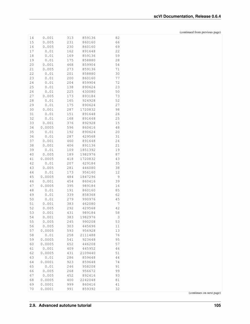
scVI Documentation, Release 0.6.4
(continued from previous page)
14 0.001 313 859136 8215 0.005 231 860160 6616 0.005 230 860160 6917 0.01 162 891648 2218 0.01 169 859136 5919 0.01 175 858880 2820 0.001 468 859904 5421 0.005 273 859136 7122 0.01 201 858880 3023 0.01 200 860160 7724 0.01 204 859904 7225 0.01 138 890624 2326 0.01 225 430080 5027 0.005 173 893184 7328 0.01 165 924928 5229 0.01 175 890624 2730 0.001 287 1720832 9831 0.01 151 891648 2632 0.01 168 891648 2533 0.001 376 892928 1534 0.0005 596 860416 4835 0.01 192 890624 2036 0.01 287 429568 3137 0.001 460 891648 2438 0.001 406 891136 2139 0.01 109 1851392 1940 0.005 189 1982976 8741 0.0005 418 1720832 4342 0.01 207 429184 3543 0.005 281 446080 3844 0.01 173 956160 1245 0.0005 484 1847296 946 0.001 454 860416 3947 0.0005 395 989184 1648 0.01 191 860160 8549 0.01 339 858368 6250 0.01 279 990976 4551 0.001 383 462080 752 0.005 292 429568 4253 0.001 431 989184 5854 0.001 383 1982976 355 0.005 245 990208 5356 0.005 303 445696 1157 0.0005 593 956928 1358 0.01 258 2111488 7659 0.0005 541 923648 9560 0.0005 652 446208 5761 0.001 409 445952 4662 0.0005 431 2109440 5163 0.01 286 859648 4464 0.0001 923 859648 7465 0.01 246 958208 9166 0.005 268 956672 9967 0.005 452 892416 9368 0.0005 400 2242048 8169 0.0001 999 860416 4170 0.0001 991 859392 32
(continues on next page)
2.9. Advanced autotune tutorial 105

scVI Documentation, Release 0.6.4
(continued from previous page)
71 0.01 321 462080 6372 0.0001 998 925952 8073 0.0001 987 1982976 474 0.0001 822 859136 3475 0.01 352 2114048 5576 0.0001 992 957696 177 0.0001 996 1719808 278 0.0001 995 2114048 6079 0.0005 585 2113024 1880 0.005 336 437120 7881 0.001 500 860160 082 0.0001 997 462720 8983 0.01 262 1720832 4084 0.01 374 454272 8385 0.0001 991 989952 9686 0.01 51 858624 5687 0.01 57 858368 7988 0.01 54 859136 3389 0.005 344 2112512 690 0.01 390 461696 1491 0.0005 608 462720 892 0.005 129 2110464 4793 0.005 115 2109440 1794 0.01 67 429568 9495 0.0005 516 923392 6496 0.005 69 991232 1097 0.0001 999 1980416 598 0.01 51 892672 8699 0.0001 40 989440 49100 0.0001 130 925184 36
[9]: brain_large_df = brain_large.get_param_df()brain_large_df.to_csv("brain_large_df")brain_large_df
[9]: marginal_ll n_layers n_hidden n_latent reconstruction_loss dropout_rate \1 138.77 1 256 8 zinb 0.12 138.779 1 256 15 zinb 0.13 138.794 1 256 11 zinb 0.14 138.798 1 256 8 zinb 0.15 138.81 1 256 10 zinb 0.16 138.828 1 256 8 zinb 0.17 138.852 1 256 8 zinb 0.18 138.894 1 256 8 zinb 0.19 138.899 1 256 8 zinb 0.110 138.902 1 256 12 zinb 0.111 138.904 1 256 12 zinb 0.112 138.91 1 256 8 zinb 0.113 138.911 1 256 9 zinb 0.114 138.914 1 256 8 zinb 0.115 138.971 1 256 8 zinb 0.116 139.126 1 128 13 nb 0.117 139.129 1 128 8 nb 0.118 139.13 2 256 13 zinb 0.119 139.141 1 256 11 zinb 0.120 139.143 1 128 13 nb 0.121 139.163 1 256 6 zinb 0.1
(continues on next page)
106 Chapter 2. Tutorials

scVI Documentation, Release 0.6.4
(continued from previous page)
22 139.19 1 256 14 nb 0.323 139.227 2 256 15 zinb 0.124 139.251 1 128 11 zinb 0.125 139.267 1 256 14 zinb 0.326 139.304 1 256 14 zinb 0.327 139.333 1 256 9 zinb 0.328 139.344 1 256 8 nb 0.329 139.422 1 64 9 zinb 0.130 139.454 2 256 8 nb 0.131 139.508 2 128 10 zinb 0.132 139.528 2 256 8 zinb 0.133 139.549 1 64 11 nb 0.134 139.59 1 64 13 nb 0.135 139.599 2 128 7 nb 0.136 139.742 3 256 11 zinb 0.137 139.749 3 256 8 zinb 0.138 139.803 3 256 14 zinb 0.139 139.825 3 256 7 zinb 0.140 139.906 1 256 7 zinb 0.541 139.953 2 128 15 zinb 0.142 139.974 1 256 5 zinb 0.543 139.975 1 256 10 zinb 0.544 139.996 1 256 5 zinb 0.545 140.024 1 64 13 zinb 0.146 140.034 2 256 6 zinb 0.347 140.093 1 256 14 nb 0.348 140.155 2 256 14 zinb 0.149 140.227 1 64 15 zinb 0.350 140.238 2 128 6 zinb 0.351 140.389 1 256 11 zinb 0.552 140.392 4 256 15 zinb 0.153 140.466 3 256 10 zinb 0.154 140.558 3 64 11 zinb 0.155 140.596 1 256 5 zinb 0.756 140.603 3 256 15 zinb 0.357 140.61 4 128 15 zinb 0.158 140.612 1 128 15 zinb 0.559 140.623 4 64 12 zinb 0.160 140.661 1 256 15 zinb 0.761 140.669 1 256 6 zinb 0.762 140.734 3 64 5 zinb 0.163 140.753 1 256 15 zinb 0.764 140.829 2 256 8 zinb 0.565 140.856 2 256 5 zinb 0.566 140.958 2 128 15 nb 0.367 141.075 2 128 5 zinb 0.568 141.513 5 128 5 zinb 0.169 141.649 5 256 12 nb 0.170 141.751 4 128 5 zinb 0.371 141.792 5 64 10 zinb 0.172 141.858 1 128 13 zinb 0.773 141.888 4 256 9 nb 0.574 141.906 3 64 9 zinb 0.175 141.927 5 256 15 nb 0.576 141.986 3 128 8 nb 0.377 142.044 5 128 9 zinb 0.578 142.138 3 64 6 nb 0.3
(continues on next page)
2.9. Advanced autotune tutorial 107

scVI Documentation, Release 0.6.4
(continued from previous page)
79 142.145 4 256 8 zinb 0.780 142.154 3 256 8 nb 0.581 142.165 1 256 15 zinb 0.982 142.172 3 128 6 nb 0.583 142.221 2 128 10 zinb 0.584 142.365 5 256 15 zinb 0.785 142.373 5 256 13 nb 0.786 142.639 5 128 6 zinb 0.787 143.32 1 64 7 nb 0.788 143.498 1 256 6 zinb 0.989 144.824 1 256 11 zinb 0.990 146.517 5 64 13 nb 0.791 146.626 5 64 11 nb 0.792 146.757 4 256 12 zinb 0.993 146.837 4 128 7 zinb 0.994 146.863 4 256 11 nb 0.995 147.011 5 256 7 zinb 0.996 147.021 2 128 12 zinb 0.997 147.024 4 64 15 zinb 0.998 147.369 4 64 11 nb 0.999 147.459 3 64 11 nb 0.9100 148.457 4 64 7 zinb 0.9
lr n_epochs n_params run index1 0.001 50 372736 672 0.001 46 376320 243 0.001 48 374272 734 0.001 45 372736 385 0.001 49 373760 706 0.001 46 372736 667 0.001 48 372736 418 0.001 42 372736 529 0.001 47 372736 2610 0.005 47 374784 6211 0.0001 47 374784 8112 0.001 49 372736 4713 0.0001 45 373248 7414 0.001 46 372736 6815 0.001 46 372736 6516 0.0005 49 187648 3317 0.001 48 186368 6418 0.0005 43 506368 7619 0.005 46 374272 9320 0.0005 49 187648 1621 0.001 47 371712 6922 0.0005 46 375808 3523 0.001 42 507392 9924 0.001 44 187136 9025 0.001 46 375808 7226 0.001 46 375808 2127 0.001 48 373248 8828 0.001 49 372736 5829 0.001 48 93312 4530 0.001 45 503808 8231 0.001 48 219648 2532 0.0001 47 503808 8933 0.0001 48 93568 97
(continues on next page)
108 Chapter 2. Tutorials

scVI Documentation, Release 0.6.4
(continued from previous page)
34 0.0005 48 93824 3735 0.0005 49 218880 3436 0.001 49 636416 9137 0.005 48 634880 3938 0.0005 48 637952 8339 0.001 44 634368 9840 0.001 48 372224 2741 0.001 46 220928 1542 0.001 43 371200 343 0.005 48 373760 8544 0.001 49 371200 2045 0.01 45 93824 8646 0.0005 44 502784 2347 0.01 47 375808 3648 0.01 38 506880 3149 0.001 48 94080 8050 0.0005 42 218624 051 0.01 47 374272 9452 0.001 46 769536 5753 0.01 49 635904 4354 0.005 49 109952 4855 0.001 48 371200 6056 0.0001 47 638464 5357 0.001 47 286464 2958 0.001 42 188160 3259 0.001 47 118272 5160 0.005 39 376320 7761 0.001 38 371712 5462 0.005 49 109184 963 0.0001 48 376320 4964 0.0005 49 503808 7165 0.0005 47 502272 2266 0.001 49 220928 1167 0.001 48 218368 2868 0.001 49 316672 7569 0.005 49 899072 1270 0.001 40 283904 9671 0.005 39 126208 5572 0.0001 48 187648 1073 0.0005 49 766464 874 0.0001 47 109696 5975 0.001 49 900608 6176 0.0005 49 251904 677 0.005 41 317696 3078 0.0005 49 109312 579 0.001 49 765952 4080 0.01 49 634880 7881 0.001 44 376320 9582 0.005 45 251392 183 0.01 30 219648 784 0.0001 49 900608 4485 0.0001 49 899584 1986 0.001 46 316928 8487 0.01 7 93056 288 0.005 3 371712 4289 0.01 0 374272 5690 0.01 17 126592 14
(continues on next page)
2.9. Advanced autotune tutorial 109

scVI Documentation, Release 0.6.4
(continued from previous page)
91 0.0005 44 126336 9292 0.001 45 768000 4693 0.001 33 284416 7994 0.001 42 767488 8795 0.01 6 896512 5096 0.001 47 220160 1397 0.001 37 118656 498 0.0001 43 118144 1899 0.0001 45 109952 17100 0.01 0 117632 63
2.9.12 Best run DataFrame
Using the previous dataframes we are able to build one containing the best results along with the results obtained withthe default parameters.
[18]: cortex_best = cortex_df.iloc[0]cortex_best.name = "Cortex tuned"cortex_default = pd.Series(
[cortex_one_shot.best_performance,1, 128, 10, "zinb", 0.1, 0.001, 400, None, None
],index=cortex_best.index
)cortex_default.name = "Cortex default"pbmc_best = pbmc_df.iloc[0]pbmc_best.name = "Pbmc tuned"pbmc_default = pd.Series(
[pbmc_one_shot.best_performance,1, 128, 10, "zinb", 0.1, 0.001, 400, None, None
],index=pbmc_best.index
)pbmc_default.name = "Pbmc default"brain_large_best = brain_large_df.iloc[0]brain_large_best.name = "Brain Large tuned"brain_large_default = pd.Series(
[brain_large_one_shot.best_performance,1, 128, 10, "zinb", 0.1, 0.001, 400, None, None
],index=brain_large_best.index
)brain_large_default.name = "Brain Large default"df_best = pd.concat(
[cortex_best,cortex_default,pbmc_best,pbmc_default,brain_large_best,brain_large_default
],axis=1
(continues on next page)
110 Chapter 2. Tutorials

scVI Documentation, Release 0.6.4
(continued from previous page)
)df_best = df_best.iloc[np.logical_not(np.isin(df_best.index, ["n_params", "run index→˓"]))]df_best
[18]: Cortex tuned Cortex default Pbmc tuned 16 GPUs \marginal_ll 1218.52 1256.03 1323.44n_layers 1 1 1n_hidden 256 128 256n_latent 10 10 14reconstruction_loss zinb zinb zinbdropout_rate 0.1 0.1 0.5lr 0.01 0.001 0.01n_epochs 248 400 170
Pbmc default Brain Large tuned Brain Large defaultmarginal_ll 1327.61 138.77 147.088n_layers 1 1 1n_hidden 128 256 128n_latent 10 8 10reconstruction_loss zinb zinb zinbdropout_rate 0.1 0.1 0.1lr 0.001 0.001 0.001n_epochs 400 50 400
2.9.13 Handy class to compare the results of each experiment
We use a second handy class to compare these results altogether. Specifically, the PlotBenchmarkable allowsto retrieve: * A DataFrame containg the runtime information of each experiment. * A DataFrame comparint thedifferent benchmarks (negative marginal LL, imputation) between tuned and default VAEs. * For each dataset, a plotaggregating the ELBO histories of each run.
[55]: from notebooks.utils.autotune_advanced_notebook import PlotBenchmarkables
[56]: tuned_benchmarkables = {"cortex": cortex,"pbmc": pbmc,"brain large": brain_large,
}one_shot_benchmarkables = {
"cortex": cortex_one_shot,"pbmc": pbmc_one_shot,"brain large": brain_large_one_shot
}plotter = PlotBenchmarkables(
tuned_benchmarkables=tuned_benchmarkables,one_shot_benchmarkables=one_shot_benchmarkables,
)
2.9. Advanced autotune tutorial 111
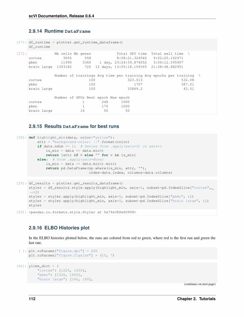
scVI Documentation, Release 0.6.4
2.9.14 Runtime DataFrame
[27]: df_runtime = plotter.get_runtime_dataframe()df_runtime
[27]: Nb cells Nb genes Total GPU time Total wall time \cortex 3005 558 8:58:21.324546 9:02:20.162471pbmc 11990 3346 1 day, 23:24:59.874052 3:04:12.595907brain large 1303182 720 12 days, 13:55:18.109345 21:38:48.882951
Number of trainings Avg time per training Avg epochs per training \cortex 100 323.013 532.08pbmc 100 1707 387.01brain large 100 10869.2 43.51
Number of GPUs Best epoch Max epochcortex 1 248 1000pbmc 1 170 1000brain large 16 50 50
2.9.15 Results DataFrame for best runs
[28]: def highlight_min(data, color="yellow"):attr = "background-color: {}".format(color)if data.ndim == 1: # Series from .apply(axis=0) or axis=1
is_min = data == data.min()return [attr if v else "" for v in is_min]
else: # from .apply(axis=None)is_min = data == data.min().min()return pd.DataFrame(np.where(is_min, attr, ""),
index=data.index, columns=data.columns)
[29]: df_results = plotter.get_results_dataframe()styler = df_results.style.apply(highlight_min, axis=0, subset=pd.IndexSlice["cortex",→˓:])styler = styler.apply(highlight_min, axis=0, subset=pd.IndexSlice["pbmc", :])styler = styler.apply(highlight_min, axis=0, subset=pd.IndexSlice["brain large", :])styler
[29]: <pandas.io.formats.style.Styler at 0x7fe38fe60908>
2.9.16 ELBO Histories plot
In the ELBO histories plotted below, the runs are colored from red to green, where red is the first run and green thelast one.
[ ]: plt.rcParams["figure.dpi"] = 200plt.rcParams["figure.figsize"] = (10, 7)
[62]: ylims_dict = {"cortex": [1225, 1600],"pbmc": [1325, 1600],"brain large": [140, 160],
(continues on next page)
112 Chapter 2. Tutorials

scVI Documentation, Release 0.6.4
(continued from previous page)
}plotter.plot_histories(figsize=(17, 5), ylims_dict=ylims_dict, filename="elbo_→˓histories_all", alpha=0.1)
2.9. Advanced autotune tutorial 113

scVI Documentation, Release 0.6.4
114 Chapter 2. Tutorials

CHAPTER
THREE
CONTRIBUTED TUTORIALS
The following tutorials have been contributed by members of the scVI user community!
3.1 Differential expression on Packer C. elegans data
This notebook was contributed by Eduardo Beltrame [@Munfred](https://github.com/Munfred) and edited by RomainLopez with help from Adam Gayoso.
Processing and visualizing 89k cells from Packer et al. 2019 C. elegans 10xv2 single cell data
Original article: A lineage-resolved molecular atlas of C. elegans embryogenesis atsingle-cell resolution
https://science.sciencemag.org/content/365/6459/eaax1971.long
The anndata object we provide has 89701 cells and 20222 genes. It includes short gene descriptions from WormBasethat will show up when mousing over the interactive plots.
3.1.1 Steps performed:
1. Loading the data from anndata containing cell labels and gene descriptions
2. Training the model with batch labels for integration with scVI
3. Retrieving the scVI latent space and imputed values
4. Visualize the latent space with an interactive UMAP plot using Plotly
5. Perform differential expression and visualize with interactive volcano plot and heatmap using Plotly
This notebook was designed to be run in Google Colab.
[ ]: # If running in Colab, navigate to Runtime -> Change runtime type# and ensure you're using a Python 3 runtime with GPU hardware accelerator# Installation of scVI in Colab can take several minutes
[ ]: import sysIN_COLAB = "google.colab" in sys.modules
show_plot = Truesave_path = "./"
(continues on next page)
115

scVI Documentation, Release 0.6.4
(continued from previous page)
if IN_COLAB:!pip install --quiet scvi[notebooks]==0.6.3
[4]: import scviscvi.__version__
[4]: '0.6.3'
[ ]: %matplotlib inline%config InlineBackend.figure_format = 'retina'# Control warningsimport warnings; warnings.simplefilter('ignore')
import osimport numpy as npimport pandas as pd
import matplotlib.pyplot as pltfrom scvi.dataset import GeneExpressionDatasetfrom scvi.models import VAEfrom scvi.inference import UnsupervisedTrainerimport torchimport anndata
import plotly.express as pximport plotly.graph_objects as go
from umap import UMAP
if IN_COLAB:%matplotlib inline
[6]: ## Change the path where the models will be savedsave_path = "./"vae_file_name = 'worm_vae.pkl'
if os.path.isfile('packer2019.h5ad'):print ("Found the data file! No need to download.")
else:print ("Downloading data...")! wget https://github.com/Munfred/wormcells-site/releases/download/packer2019/
→˓packer2019.h5ad
Found the data file! No need to download.
[ ]: adata = anndata.read('packer2019.h5ad')
[8]: adata
[8]: AnnData object with n_obs × n_vars = 89701 × 20222obs: 'cell', 'numi', 'time_point', 'batch', 'size_factor', 'cell_type', 'cell_
→˓subtype', 'plot_cell_type', 'raw_embryo_time', 'embryo_time', 'embryo_time_bin',→˓'raw_embryo_time_bin', 'lineage', 'passed_qc'
var: 'gene_id', 'gene_name', 'gene_description'
116 Chapter 3. Contributed tutorials

scVI Documentation, Release 0.6.4
[9]: adata.X
[9]: <89701x20222 sparse matrix of type '<class 'numpy.float32'>'with 82802059 stored elements in Compressed Sparse Column format>
Take a look at the gene descriptions
The gene descriptions were taken using the WormBase API.
[10]: display(adata.var.head().style.set_properties(subset=['gene_description'], **{'width':→˓ '600px'}))
<pandas.io.formats.style.Styler at 0x7fd27a960588>
[11]: adata.obs.head().T
[11]: index AAACCTGAGACAATAC-300.1.1 ... AAACCTGCAAGACGTG-300.1.1cell AAACCTGAGACAATAC-300.1.1 ... AAACCTGCAAGACGTG-300.1.1numi 1630 ... 1003time_point 300_minutes ... 300_minutesbatch Waterston_300_minutes ... Waterston_300_minutessize_factor 1.02319 ... 0.62961cell_type Body_wall_muscle ... Ciliated_amphid_neuroncell_subtype BWM_head_row_1 ... AFDplot_cell_type BWM_head_row_1 ... AFDraw_embryo_time 360 ... 350embryo_time 380 ... 350embryo_time_bin 330-390 ... 330-390raw_embryo_time_bin 330-390 ... 330-390lineage MSxpappp ... ABalpppapav/ABpraaaapavpassed_qc True ... True
[14 rows x 5 columns]
3.1.2 Loading data
We load the Packer data and use the batch annotations for scVI. Here, each experiment correspond to a batch.
[12]: gene_dataset = GeneExpressionDataset()
# we provide the `batch_indices` so that scvi can perform batch correctiongene_dataset.populate_from_data(
adata.X,gene_names=adata.var.index.values,cell_types=adata.obs['cell_type'].values,batch_indices=adata.obs['batch'].cat.codes.values,)
# We select the 1000 most variable genes, which is a recommended selection criteria→˓of scvi# this method in particular is based on the method of Seurat v3gene_dataset.subsample_genes(1000)sel_genes = gene_dataset.gene_names
3.1. Differential expression on Packer C. elegans data 117

scVI Documentation, Release 0.6.4
[2020-04-02 03:49:05,753] INFO - scvi.dataset.dataset | Remapping labels to [0,N][2020-04-02 03:49:05,759] INFO - scvi.dataset.dataset | Remapping batch_indices to [0,→˓N][2020-04-02 03:49:05,765] INFO - scvi.dataset.dataset | extracting highly variable→˓genes using seurat_v3 flavor
Transforming to str index.
[2020-04-02 03:49:56,429] INFO - scvi.dataset.dataset | Downsampling from 20222 to→˓1000 genes[2020-04-02 03:49:56,775] INFO - scvi.dataset.dataset | Computing the library size→˓for the new data[2020-04-02 03:49:57,163] INFO - scvi.dataset.dataset | Filtering non-expressing→˓cells.[2020-04-02 03:49:57,579] INFO - scvi.dataset.dataset | Computing the library size→˓for the new data[2020-04-02 03:49:57,965] INFO - scvi.dataset.dataset | Downsampled from 89701 to→˓89701 cells
At this point we may make the scVI dataset RNA count matrix dense, as we filtered the genes. This makes inferencefaster because when the matrix is sparse, the trainer has to make each minibatch dense before it loads it on the modeland the GPU is using CUDA.
[13]: gene_dataset.X = gene_dataset.X.toarray()
[2020-04-02 03:50:00,523] INFO - scvi.dataset.dataset | Computing the library size→˓for the new data
[14]: adata.obs['cell_type'].values
[14]: [Body_wall_muscle, nan, nan, Body_wall_muscle, Ciliated_amphid_neuron, ..., Rectal_→˓gland, nan, nan, nan, nan]Length: 89701Categories (37, object): [ABarpaaa_lineage, Arcade_cell, Body_wall_muscle, Ciliated_→˓amphid_neuron, ...,
hmc_and_homolog, hmc_homolog, hyp1V_and_ant_arc_V, nan]
3.1.3 Training
• n_epochs: Maximum number of epochs to train the model. If the likelihood change is small than a set thresholdtraining will stop automatically.
• lr: learning rate. Set to 0.001 here.
• use_cuda: Set to true to use CUDA (GPU required)
[ ]: # for this dataset 50 epochs is sufficient# note that smaller datasets require hundreds of epochsn_epochs = 50lr = 1e-3use_cuda = True
We now create the model and the trainer object. We train the model and output model likelihood every epoch. In orderto evaluate the likelihood on a test set, we split the datasets (the current code can also so train/validation/test).
If a pre-trained model already exist in the save_path then load the same model rather than re-training it. This isparticularly useful for large datasets.
118 Chapter 3. Contributed tutorials
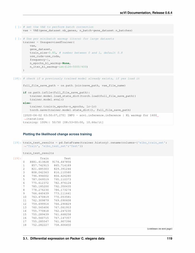
scVI Documentation, Release 0.6.4
[ ]: # set the VAE to perform batch correctionvae = VAE(gene_dataset.nb_genes, n_batch=gene_dataset.n_batches)
[ ]: # Use per minibatch warmup (iters) for large datasetstrainer = UnsupervisedTrainer(
vae,gene_dataset,train_size=0.85, # number between 0 and 1, default 0.8use_cuda=use_cuda,frequency=1,n_epochs_kl_warmup=None,n_iter_kl_warmup=int(128*5000/400)
)
[18]: # check if a previously trained model already exists, if yes load it
full_file_save_path = os.path.join(save_path, vae_file_name)
if os.path.isfile(full_file_save_path):trainer.model.load_state_dict(torch.load(full_file_save_path))trainer.model.eval()
else:trainer.train(n_epochs=n_epochs, lr=lr)torch.save(trainer.model.state_dict(), full_file_save_path)
[2020-04-02 03:50:07,270] INFO - scvi.inference.inference | KL warmup for 1600→˓iterationstraining: 100%|| 50/50 [08:53<00:00, 10.66s/it]
Plotting the likelihood change across training
[19]: train_test_results = pd.DataFrame(trainer.history).rename(columns={'elbo_train_set':→˓'Train', 'elbo_test_set':'Test'})
train_test_results
[19]: Train Test0 8881.413828 9174.4478561 857.742913 865.7141892 821.685303 829.3912463 808.042363 816.1105804 796.994002 804.4262805 787.069519 795.1103736 775.612372 782.9761247 785.185200 792.3504358 778.276230 786.1732749 766.440439 773.11164110 763.470819 770.05358111 762.309879 769.09060812 759.699914 766.29082913 760.565406 767.06195314 755.770818 762.24723015 755.289439 761.66825816 760.560715 767.14735717 755.285547 761.90739618 752.282227 758.606450
(continues on next page)
3.1. Differential expression on Packer C. elegans data 119

scVI Documentation, Release 0.6.4
(continued from previous page)
19 752.231292 758.70757220 751.001023 757.31801021 750.882924 757.27063022 753.712712 760.24856323 752.402924 759.03868424 750.010072 756.42461325 751.233984 757.74138926 748.450227 754.82712427 752.164061 758.74030228 748.442852 754.91677329 753.610544 760.39384530 748.497168 755.02903631 749.499188 756.38885732 748.662938 755.37915333 747.743216 754.30486534 747.289906 753.93862635 746.901389 753.52791436 747.174424 753.74779837 746.882975 753.54408238 746.582319 753.28605539 747.826352 754.54304340 747.763953 754.59998041 746.903656 753.51866342 746.093606 752.91451343 747.682025 754.57708144 748.042126 754.90875145 746.043148 752.92092946 745.559933 752.40847747 745.672933 752.53376848 748.517461 755.66753949 745.237304 752.20567650 745.312490 752.293802
[20]: ax = train_test_results.plot()ax.set_xlabel("Epoch")ax.set_ylabel("Error")plt.show()
120 Chapter 3. Contributed tutorials

scVI Documentation, Release 0.6.4
3.1.4 Obtaining the posterior object and sample latent space
The posterior object contains a model and a gene_dataset, as well as additional arguments that for Pytorch’sDataLoader. It also comes with many methods or utilities querying the model, such as differential expression,imputation and differential analyisis.
To get an ordered output result, we might use .sequential posterior’s method which return another instance ofposterior (with shallow copy of all its object references), but where the iteration is in the same ordered as its indicesattribute.
[21]: # This provides a posterior with sequential index samplingfull = trainer.create_posterior()latent, batch_indices, labels = full.get_latent()batch_indices = batch_indices.ravel()latent.shape
[21]: (89701, 10)
[22]: # store the latent space in a new anndata objectpost_adata = anndata.AnnData(X=gene_dataset.X)post_adata.obs=adata.obspost_adata.obsm["latent"] = latentpost_adata
[22]: AnnData object with n_obs × n_vars = 89701 × 1000obs: 'cell', 'numi', 'time_point', 'batch', 'size_factor', 'cell_type', 'cell_
→˓subtype', 'plot_cell_type', 'raw_embryo_time', 'embryo_time', 'embryo_time_bin',→˓'raw_embryo_time_bin', 'lineage', 'passed_qc'
obsm: 'latent'
Using Plotly’s Scattergl we can easily and speedily make interactive plots with 89k cells!
[ ]: # here's a hack to randomize categorical colors, since plotly can't do that in a→˓straightforward manner# we take the list of named css colors that it recognizes, and we picked a color→˓based on the code of# the cluster we are coloringcss_colors=['aliceblue','antiquewhite','aqua','aquamarine','azure','bisque','black',→˓'blanchedalmond','blue','blueviolet','brown','burlywood','cadetblue','chartreuse','chocolate','coral',→˓'cornflowerblue','crimson','cyan','darkblue','darkcyan','darkgoldenrod','darkgray','darkgrey',→˓'darkgreen','darkkhaki','darkmagenta','darkolivegreen','darkorange','darkorchid','darkred','darksalmon',→˓'darkseagreen','darkslateblue','darkslategray','darkslategrey','darkturquoise','darkviolet','deeppink→˓','deepskyblue','dimgray','dimgrey','dodgerblue','firebrick','floralwhite','forestgreen','fuchsia',→˓'gainsboro','ghostwhite','gold','goldenrod','gray','grey','green','greenyellow','honeydew','hotpink','indianred→˓','indigo','ivory','khaki','lavender','lavenderblush','lawngreen','lemonchiffon','lightblue',→˓'lightcoral','lightcyan','lightgoldenrodyellow','lightgray','lightgrey','lightgreen','lightpink','lightsalmon',→˓'lightseagreen','lightskyblue','lightslategray','lightslategrey','lightsteelblue','lightyellow','lime→˓','limegreen','linen', (continues on next page)
3.1. Differential expression on Packer C. elegans data 121

scVI Documentation, Release 0.6.4
(continued from previous page)
'magenta','maroon','mediumaquamarine','mediumblue','mediumorchid','mediumpurple',→˓'mediumseagreen','mediumslateblue','mediumspringgreen','mediumturquoise','mediumvioletred',→˓'midnightblue','mintcream','mistyrose','moccasin','navajowhite','navy','oldlace','olive','olivedrab','orange',→˓'orangered','orchid','palegoldenrod','palegreen','paleturquoise','palevioletred','papayawhip','peachpuff',→˓'peru','pink','plum','powderblue','purple','red','rosybrown','royalblue','saddlebrown','salmon',→˓'sandybrown','seagreen','seashell','sienna','silver','skyblue','slateblue','slategray','slategrey','snow',→˓'springgreen','steelblue','tan','teal','thistle','tomato','turquoise','violet','wheat','white','whitesmoke',→˓'yellow','yellowgreen']
# we just repeat the list of colors a bunch of times to ensure we always have more→˓colors than clusterscss_colors = css_colors*100
# now define a function to plot any embedding
def plot_embedding(embedding_kind, # the embedding must be a label in→˓the post_adata.obsm
adata=adata, # the original adata for taking the→˓cluster labels
post_adata=post_adata,cluster_feature ='cell_type',xlabel="Dimension 1",ylabel="Dimension 2",plot_title="Embedding on single cell data"):
# `cluster_feature` should be the name of one of the categorical annotation→˓columns
# e.g. `cell_type`, `cell_subtype`, `time_point`
cluster_ids = adata.obs[cluster_feature].cat.codes.unique()id_to_cluster_map = dict( zip( adata.obs[cluster_feature].cat.codes, adata.
→˓obs[cluster_feature] ) )cluster_to_id_map = dict([[v,k] for k,v in id_to_cluster_map.items()])
fig = go.Figure()for _cluster_id in adata.obs[cluster_feature].cat.codes.unique():
fig.add_trace(go.Scattergl(
x = post_adata.obsm[embedding_kind][:,0][post_adata.obs[cluster_→˓feature].cat.codes==_cluster_id]
, y = post_adata.obsm[embedding_kind][:,1][post_adata.obs[cluster_→˓feature].cat.codes==_cluster_id]
, mode='markers', marker=dict(
# we randomize colors by starting at a random place in the list→˓of named css colors
color=css_colors[_cluster_id+np.random.randint(0,len(np.→˓unique(css_colors)))]
, size = 3)
(continues on next page)
122 Chapter 3. Contributed tutorials

scVI Documentation, Release 0.6.4
(continued from previous page)
, showlegend=True, name=id_to_cluster_map[_cluster_id], hoverinfo=['name'])
)
layout={"title": {"text": plot_title
, 'x':0.5}
, 'xaxis': {'title': {"text": xlabel}}, 'yaxis': {'title': {"text": ylabel}}, "height": 800, "width":1000
}fig.update_layout(layout)fig.update_layout(showlegend=True)return fig
[ ]: latent_umap = UMAP(spread=2).fit_transform(latent)
[ ]: post_adata.obsm["UMAP"] = np.array(latent_umap)
[ ]: fig = plot_embedding(embedding_kind='UMAP',cluster_feature ='cell_type',xlabel="UMAP 1",ylabel="UMAP 2",plot_title="UMAP on scVI latent space for Packer C. elegans single
→˓cell data")
[27]: # uncomment this line to save an interactive html plot, in case it is not rendering#fig.write_html('worms_interactive_tsne.html')fig.show()
Performing Differential Expression with vanilla and change modes
Note: scVI recently introduced a second way to perform DE, and some functions and documentation are stillchanging. The old mode is called ``vanilla`` and is performed below. The new mode is called ``change`` and isdone at the end of the notebook. In addition to Bayes Factors, the new ``change`` mode allows for calculatingp-values, which are more commonly seen in volcano plots.
• From the trained VAE model we can sample the gene expression rate for each gene in each cell.
• For two populations of interest, we can then randomly sample pairs of cells, one from each population tocompare their expression rate for a gene.
• In the vanilla mode, DE is measured by logit(p/(1-p)) where p is the probability of a cell from population Ahaving a higher expression than a cell from population B.
• We can form the null distribution of the DE values by sampling pairs randomly from the combined population.
3.1. Differential expression on Packer C. elegans data 123

scVI Documentation, Release 0.6.4
Explanation of Vanilla DE mode and Bayes Factors
Explanation adapted from the scVi `differential_expression_score docstring <https://github.com/YosefLab/scVI/blob/05920d1f85daa362d4fb694e588ab090bc84e207/scvi/inference/posterior.py#L640>`__.
The ``vanilla`` mode follows protocol described in Lopez et al, arXiv:1709.02082.
In this case for a given gene we perform hypothesis testing based on latent variable in the generative model that modelsthe mean of the gene expression.
We are comparing ℎ1𝑔 , the mean expression of gene 𝑔 in cell type 1, with ℎ2𝑔 , the mean expression of 𝑔 in cell type 2.
The hypotheses are:
𝑀𝑔1 : ℎ1𝑔 > ℎ2𝑔
𝑀𝑔2 : ℎ1𝑔 ≤ ℎ2𝑔
DE between cell types 1 and 2 for each gene can then be based on the Bayes factors:
Natural Log Bayes Factor for gene g in cell types 1 and 2 = ln(𝐵𝐹 𝑔12) = ln(
𝑝(𝑀𝑔1 |𝑥1, 𝑥2)
𝑝(𝑀𝑔2 |𝑥1, 𝑥2)
)
Note that the scvi ``differential_expression_score`` returns the *natural logarithm* of the Bayes Factor. This is:math:`ln(BF_{10})` in the table discussed below.
To compute the gene specific Bayes factors using masks idx1 and idx2 we sample the Posterior in the following way:
1. The posterior is sampled n_samples times for each subpopulation
2. For computation efficiency (posterior sampling is quite expensive), instead of comparing element-wise the ob-tained samples, we can permute posterior samples.
Remember that computing the Bayes Factor requires sampling 𝑞(𝑧𝐴|𝑥𝐴) and 𝑞(𝑧𝐵 |𝑥𝐵)
Interpreting Bayes factors
To learn more about Bayes factors vs. p-values, see the review On p-Values and Bayes Factors by Leonhard Held andManuela Ott.
For a shorter overview, see this blog post. A common interpretation table is copied below.In our notation, 𝐵𝐹10 is 𝐵𝐹 𝑔
12, 𝐻0 is 𝑀𝑔1 and 𝐻1 is 𝑀𝑔
2
Bayes factor 𝐵𝐹10 ln(𝐵𝐹10) Interpretation> 100 > 4.60 Extreme evidence for H130 – 100 (3.4, 4.6) Very strong evidence for H110 – 30 (2.3, 3.4) Strong evidence for H13 – 10 (1.1, 2.3) Moderate evidence for H11 – 3 (0 , 1.1) Anecdotal evidence for H11 0 No evidence1/3 – 1 (-1.1, 0) Anecdotal evidence for H01/3 – 1/10 (-2.30, -1.1) Moderate evidence for H01/10 – 1/30 (-3.4, -2.30) Strong evidence for H01/30 – 1/100 (-4.6, -3.4) Very strong evidence for H0< 1/100 < -4.6 Extreme evidence for H0
124 Chapter 3. Contributed tutorials

scVI Documentation, Release 0.6.4
3.1.5 Selecting cells to compare
[28]: # let's take a look at abundances of different cell typesadata.obs['cell_type'].value_counts()
[28]: nan 35052Body_wall_muscle 17520Hypodermis 7746Ciliated_amphid_neuron 6090Ciliated_non_amphid_neuron 4468Seam_cell 2766Pharyngeal_muscle 2562Glia 1857Intestine 1732Pharyngeal_neuron 1471Pharyngeal_marginal_cell 911Coelomocyte 787Pharyngeal_gland 786GLR 768Intestinal_and_rectal_muscle 568Germline 499Pharyngeal_intestinal_valve 493Arcade_cell 434Z1_Z4 372Rectal_cell 327M_cell 315ABarpaaa_lineage 273Rectal_gland 265Excretory_cell 215Excretory_gland 205hmc 189hmc_homolog 155T 141hmc_and_homolog 122Parent_of_exc_gland_AVK 114hyp1V_and_ant_arc_V 112Excretory_duct_and_pore 91Parent_of_hyp1V_and_ant_arc_V 75G2_and_W_blasts 72Excretory_cell_parent 62Parent_of_exc_duct_pore_DB_1_3 61XXX 25Name: cell_type, dtype: int64
[29]: # let's pick two cell typescell_type_1 = 'Ciliated_non_amphid_neuron'cell_type_2 = 'Intestine'
cell_idx1 = adata.obs['cell_type'] == cell_type_1print(sum(cell_idx1), 'cells of type', cell_type_1)cell_idx2 = adata.obs['cell_type'] == cell_type_2print(sum(cell_idx2), 'cells of type', cell_type_2)
4468 cells of type Ciliated_non_amphid_neuron1732 cells of type Intestine
3.1. Differential expression on Packer C. elegans data 125
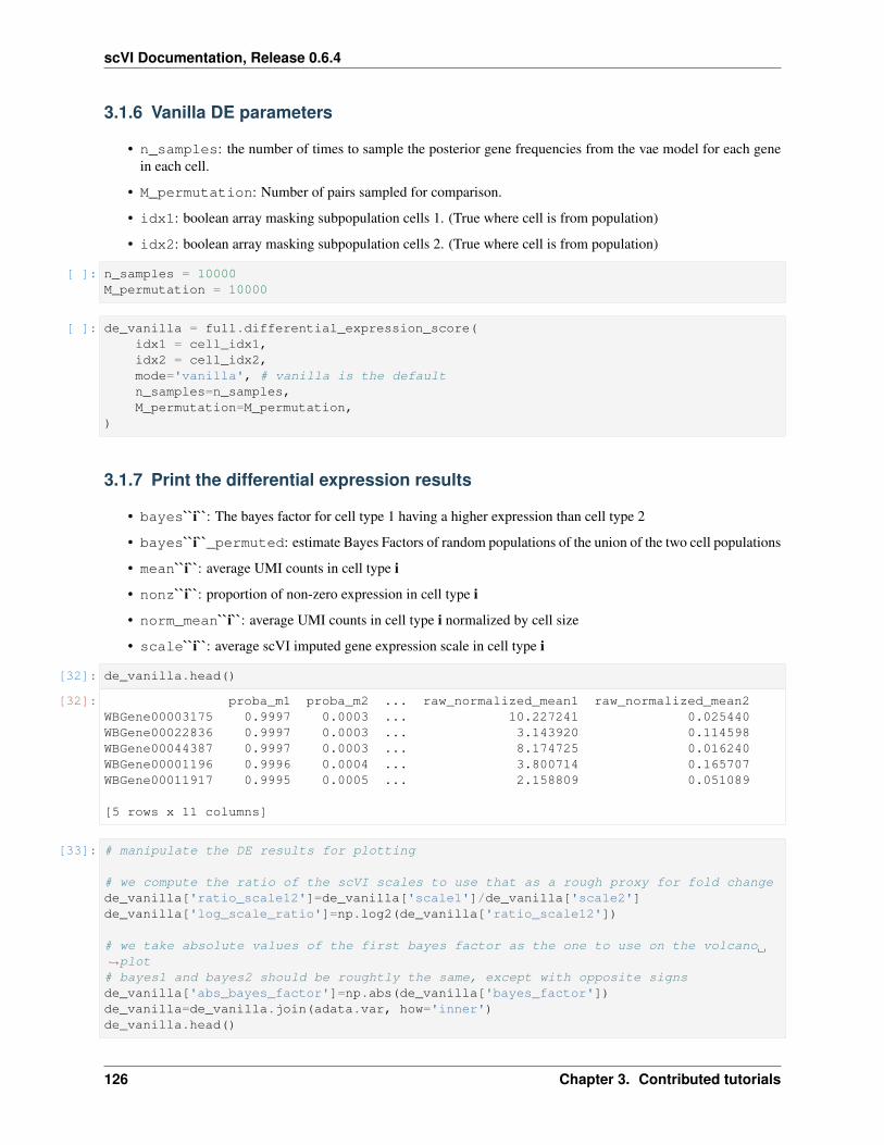
scVI Documentation, Release 0.6.4
3.1.6 Vanilla DE parameters
• n_samples: the number of times to sample the posterior gene frequencies from the vae model for each genein each cell.
• M_permutation: Number of pairs sampled for comparison.
• idx1: boolean array masking subpopulation cells 1. (True where cell is from population)
• idx2: boolean array masking subpopulation cells 2. (True where cell is from population)
[ ]: n_samples = 10000M_permutation = 10000
[ ]: de_vanilla = full.differential_expression_score(idx1 = cell_idx1,idx2 = cell_idx2,mode='vanilla', # vanilla is the defaultn_samples=n_samples,M_permutation=M_permutation,
)
3.1.7 Print the differential expression results
• bayes``i``: The bayes factor for cell type 1 having a higher expression than cell type 2
• bayes``i``_permuted: estimate Bayes Factors of random populations of the union of the two cell populations
• mean``i``: average UMI counts in cell type i
• nonz``i``: proportion of non-zero expression in cell type i
• norm_mean``i``: average UMI counts in cell type i normalized by cell size
• scale``i``: average scVI imputed gene expression scale in cell type i
[32]: de_vanilla.head()
[32]: proba_m1 proba_m2 ... raw_normalized_mean1 raw_normalized_mean2WBGene00003175 0.9997 0.0003 ... 10.227241 0.025440WBGene00022836 0.9997 0.0003 ... 3.143920 0.114598WBGene00044387 0.9997 0.0003 ... 8.174725 0.016240WBGene00001196 0.9996 0.0004 ... 3.800714 0.165707WBGene00011917 0.9995 0.0005 ... 2.158809 0.051089
[5 rows x 11 columns]
[33]: # manipulate the DE results for plotting
# we compute the ratio of the scVI scales to use that as a rough proxy for fold changede_vanilla['ratio_scale12']=de_vanilla['scale1']/de_vanilla['scale2']de_vanilla['log_scale_ratio']=np.log2(de_vanilla['ratio_scale12'])
# we take absolute values of the first bayes factor as the one to use on the volcano→˓plot# bayes1 and bayes2 should be roughtly the same, except with opposite signsde_vanilla['abs_bayes_factor']=np.abs(de_vanilla['bayes_factor'])de_vanilla=de_vanilla.join(adata.var, how='inner')de_vanilla.head()
126 Chapter 3. Contributed tutorials

scVI Documentation, Release 0.6.4
[33]: proba_m1 ... gene_descriptionWBGene00003175 0.9997 ... Is an ortholog of human TUBA1A (tubulin alpha ...WBGene00022836 0.9997 ... Is an ortholog of human TMX3. Is predicted to ...WBGene00044387 0.9997 ... Is enriched in intestine and nervous system ba...WBGene00001196 0.9996 ... Is an ortholog of human GNAQ (G protein subuni...WBGene00011917 0.9995 ... Is an ortholog of human TXLNA (taxilin alpha)...
[5 rows x 17 columns]
Because we’re using the vanilla mode, note that this volcano plot shows the ratios of the scVI expression scale of thetwo tissues vs the absolute value of the natural log bayes factor.
The new change mode allows for calculating log fold change and p-values, which are more commonly seen involcano plots
We can highlight genes of interest based on simple string matching. For example, the cell below highlights all C.elegans neuropeptides (whose name conveniently all start with nlp, ins or flp). Other genes with be a transparentgray dot.
[ ]: de_vanilla['gene_color'] = 'rgba(100, 100, 100, 0.25)'de_vanilla.loc[de_vanilla['gene_name'].str.contains('ins-'), 'gene_color'] =→˓'rgba(255, 1,0, 1)'de_vanilla.loc[de_vanilla['gene_name'].str.contains('nlp-'), 'gene_color'] =→˓'rgba(255, 0,0, 1)'de_vanilla.loc[de_vanilla['gene_name'].str.contains('flp-'), 'gene_color'] =→˓'rgba(255, 0,1, 1)'
[35]: # first we create these variables to customize the hover text in plotly's heatmap# the text needs to be arranged in a matrix the same shape as the heatmap# for the gene descriptions text, which can be several sentences, we add a line break→˓after each sentencede_vanilla['gene_description_html'] = de_vanilla['gene_description'].str.replace('\.→˓', '.<br>')
fig = go.Figure(data=go.Scatter(
x=de_vanilla["log_scale_ratio"].round(3), y=de_vanilla["abs_bayes_factor"].round(3), mode='markers', marker=dict(color=de_vanilla['gene_color']), hoverinfo='text', text=de_vanilla['gene_description_html'], customdata=de_vanilla.gene_id.values + '<br>Name: ' + de_
→˓vanilla.gene_name.values, hovertemplate='%{customdata} <br>' +
'|ln(BF)|: %{y}<br>' +'Log2 scale ratio: %{x}' +'<extra>%{text}</extra>'
), layout= {
"title": {"text":"Vanilla differential expression of Packer
→˓C. elegans data between <br> <b>" +str(cell_type_1) + "</b> and <b>" +
→˓str(cell_type_2) + " ", 'x':0.5
(continues on next page)
3.1. Differential expression on Packer C. elegans data 127

scVI Documentation, Release 0.6.4
(continued from previous page)
}, 'xaxis': {'title': {"text": "Log2 of scVI
→˓expression scale"}}, 'yaxis': {'title': {"text": "Absolute value of
→˓natural log of Bayes Factor"}}}
)# uncomment line below to save the interactive volcano plot as html# fig.write_html('worms_interactive_volcano_plot_vanilla_DE.html')fig.show()
3.1.8 Heatmap of top expressed genes for vanilla mode
Now we perform DE between each cell type vs all other cells and make a heatmap of the result.
First we need to make cell type sumary with numerical codes for each cell type
[36]: # we need to numerically encode the cell types for passing the cluster identity to→˓scVIcell_code_to_type = dict( zip( adata.obs['cell_type'].cat.codes, adata.obs['cell_type→˓'] ) )cell_type_to_code_map = dict([[v,k] for k,v in cell_code_to_type.items()])# check that we got unique cell type labelsassert len(cell_code_to_type)==len(cell_type_to_code_map)
cell_types_summary=pd.DataFrame(index=adata.obs['cell_type'].value_counts().index)cell_types_summary['cell_type_code']=cell_types_summary.index.map(cell_type_to_code_→˓map)cell_types_summary['ncells']=adata.obs['cell_type'].value_counts()cell_types_summary['cell_type_name']=adata.obs['cell_type'].value_counts().indexcell_types_summary.to_csv('packer_cell_types_summary.csv')cell_types_summary.head()
[36]: cell_type_code ncells cell_type_namenan 36 35052 nanBody_wall_muscle 2 17520 Body_wall_muscleHypodermis 14 7746 HypodermisCiliated_amphid_neuron 3 6090 Ciliated_amphid_neuronCiliated_non_amphid_neuron 4 4468 Ciliated_non_amphid_neuron
[37]: # create a column in the cell data with the cluster id each cell belongs toadata.obs['cell_type_code'] = adata.obs['cell_type'].cat.codes
# this returns a list of dataframes with DE results (one for each cluster),# and a list with the corresponding cluster idvanilla_per_cluster_de, vanilla_cluster_id = full.one_vs_all_degenes(
cell_labels=adata.obs['cell_type_code'].ravel(),mode = 'vanilla', # vanilla is the default modemin_cells=1)
HBox(children=(IntProgress(value=0, max=37), HTML(value='')))
128 Chapter 3. Contributed tutorials

scVI Documentation, Release 0.6.4
[ ]: # pick the top 10 genes in each clustervanilla_top_genes = []for x in vanilla_per_cluster_de:
vanilla_top_genes.append(x[:10])vanilla_top_genes = pd.concat(vanilla_top_genes)vanilla_top_genes = np.unique(vanilla_top_genes.index)
[39]: # fetch the expression values for the top 10 genesvanilla_top_expression = [x.filter(items=vanilla_top_genes, axis=0)['scale1'] for x→˓in vanilla_per_cluster_de]vanilla_top_expression = pd.concat(vanilla_top_expression, axis=1)vanilla_top_expression = np.log10(1 + vanilla_top_expression)cluster_name = [cell_code_to_type[_id] for _id in vanilla_cluster_id]vanilla_top_expression.columns=cluster_name
# convert into anndata object to tie with more metadata, such as gene names and→˓descriptionsvanilla_top_expression = anndata.AnnData(vanilla_top_expression.T)vanilla_top_expression.obs = vanilla_top_expression.obs.join(cell_types_summary)vanilla_top_expression.obs.head()
[39]: cell_type_code ncells cell_type_nameABarpaaa_lineage 0 273 ABarpaaa_lineageArcade_cell 1 434 Arcade_cellBody_wall_muscle 2 17520 Body_wall_muscleCiliated_amphid_neuron 3 6090 Ciliated_amphid_neuronCiliated_non_amphid_neuron 4 4468 Ciliated_non_amphid_neuron
[40]: #make a copy of the annotated gene metadata with gene ids all lower case to avoid→˓problems when joining dataframesadata_var_lowcase = adata.var.copy()adata_var_lowcase.index = adata_var_lowcase.index.str.lower()
#convert top_expression gene ids index to lowercase for joining with metadatavanilla_top_expression.var.index = vanilla_top_expression.var.index.str.lower()vanilla_top_expression.var=vanilla_top_expression.var.join(adata_var_lowcase)
vanilla_top_expression.var.index=vanilla_top_expression.var['gene_id']vanilla_top_expression.var.head().style.set_properties(subset=['gene_description'], **→˓{'width': '600px'})
[40]: <pandas.io.formats.style.Styler at 0x7fd1f2657d68>
3.1.9 Create interactive heatmap for vanilla results
In this heatmap we plot the top 10 genes for each of the 37 annotated tissue types.
[41]: # first we create these variables to customize the hover text in plotly's heatmap# the text needs to be arranged in a matrix the same shape as the heatmap# for the gene descriptions text, which can be several sentences, we add a line break→˓after each sentencevanilla_top_expression.var['gene_description_html'] = vanilla_top_expression.var[→˓'gene_description'].str.replace('\. ', '.<br>')gene_description_text_matrix = np.tile(vanilla_top_expression.var['gene_description_→˓html'].values, (len(vanilla_top_expression.obs['cell_type_name']),1) )gene_ids_text_matrix = np.tile(vanilla_top_expression.var['gene_id'].values,→˓(len(vanilla_top_expression.obs['cell_type_name']),1)) (continues on next page)
3.1. Differential expression on Packer C. elegans data 129

scVI Documentation, Release 0.6.4
(continued from previous page)
# now create the heatmap with plotlyfig = go.Figure(
data=go.Heatmap(z=np.log(vanilla_top_expression.X * 10000), # multiply by
→˓10000 to interpret this as ln(CP10K) scalex=vanilla_top_expression.var['gene_name'],y=vanilla_top_expression.obs['cell_type_name'],hoverinfo='text',text=gene_description_text_matrix,customdata=gene_ids_text_matrix,hovertemplate='%{customdata} <br>Name: %{x}<br>Cell type: %{y}
→˓<br>ln(CP10K) %{z} <extra>%{text}</extra>',),
layout= {"title": {"text": "Vanilla differential expression of Packer
→˓C. elegans single cell data"},"height": 800,},
)
# uncomment line below to save the interactive volcano plot as html# fig.write_html('worms_interactive_heatmap_vanilla_DE.html')fig.show()
Now we perform differential expression using the change DE mode introduced in scVI v0.60
The ``change`` mode follows the protocol described in Boyeau et al, bioRxiv 2019. doi: 10.1101/794289
It consists in estimating an effect size random variable (e.g., log fold-change) and performing Bayesian hypothesistesting on this variable.
The new change_fn function computes the effect size variable r based two inputs corresponding to the normalizedmeans in both populations
𝑀1 : 𝑟 ∈ 𝑅0 (effect size r in region inducing differential expression)
𝑀2 : 𝑟 /∈ 𝑅0 (no differential expression)
To characterize the region 𝑅0, the user has two choices.
A common case is when the region [−𝛿, 𝛿] does not induce differential expression.
If the user specifies a threshold delta, we suppose that 𝑅0 = R∖[−𝛿, 𝛿]
Specify an specific indicator function $ 1 : R ↦→ ‘0, 1 : 𝑛𝑏𝑠𝑝ℎ𝑖𝑛𝑥−𝑚𝑎𝑡ℎ : 𝑡𝑒𝑥𝑡{𝑠.𝑡.}‘𝑟 ∈ ‘𝑅_0 : 𝑛𝑏𝑠𝑝ℎ𝑖𝑛𝑥−𝑚𝑎𝑡ℎ :𝑖𝑓𝑓 :nbsphinx-math:𝑚𝑎𝑡ℎ𝑏𝑏{1}‘(𝑟) = 1$
Decision-making can then be based on the estimates of 𝑝(𝑀1|𝑥1, 𝑥2)
[ ]: de_change = full.differential_expression_score(idx1 = cell_idx1, # we use the same cells as chosen beforeidx2 = cell_idx2,mode='change', # set to the new change moden_samples=n_samples,M_permutation=M_permutation,
)
130 Chapter 3. Contributed tutorials

scVI Documentation, Release 0.6.4
[43]: de_change.head()
[43]: proba_de ... raw_normalized_mean2WBGene00044387 1.0000 ... 0.016240WBGene00044705 0.9998 ... 0.002663WBGene00009741 0.9998 ... 1.669146WBGene00003175 0.9998 ... 0.025440WBGene00000433 0.9997 ... 0.011383
[5 rows x 16 columns]
[44]: # manipulate the DE results for plotting
# we use the `mean` entru in de_chage, it is the scVI posterior log2 fold changede_change['log10_pvalue']=np.log10(de_change['proba_not_de'])
# we take absolute values of the first bayes factor as the one to use on the volcano→˓plot# bayes1 and bayes2 should be roughtly the same, except with opposite signsde_change['abs_bayes_factor']=np.abs(de_change['bayes_factor'])de_change=de_change.join(adata.var, how='inner')de_change.head()
[44]: proba_de ... gene_descriptionWBGene00044387 1.0000 ... Is enriched in intestine and nervous system ba...WBGene00044705 0.9998 ... Is an ortholog of human PPIL6 (peptidylprolyl ...WBGene00009741 0.9998 ... Is enriched in OLL; PVD; intestine; and pharyn...WBGene00003175 0.9998 ... Is an ortholog of human TUBA1A (tubulin alpha ...WBGene00000433 0.9997 ... Is an ortholog of human DRGX (dorsal root gang...
[5 rows x 21 columns]
3.1.10 Volcano plot of change mode DE with p-values
In addition to Bayes Factors, the new change mode allows for calculating log fold change and p-values, which aremore commonly seen in volcano plots.
We can highlight genes of interest based on simple string matching. For example, the cell below highlights all C.elegans neuropeptides (whose name conveniently all start with nlp, ins or flp). Other genes with be a transparentgray dot.
[ ]: de_change['gene_color'] = 'rgba(100, 100, 100, 0.25)'de_change.loc[de_change['gene_name'].str.contains('ins-'), 'gene_color'] = 'rgba(255,→˓1,0, 1)'de_change.loc[de_change['gene_name'].str.contains('nlp-'), 'gene_color'] = 'rgba(255,→˓0,0, 1)'de_change.loc[de_change['gene_name'].str.contains('flp-'), 'gene_color'] = 'rgba(255,→˓0,1, 1)'
[46]: # first we create these variables to customize the hover text in plotly's heatmap# the text needs to be arranged in a matrix the same shape as the heatmap# for the gene descriptions text, which can be several sentences, we add a line break→˓after each sentencede_change['gene_description_html'] = de_change['gene_description'].str.replace('\. ',→˓'.<br>')
(continues on next page)
3.1. Differential expression on Packer C. elegans data 131
scVI Documentation, Release 0.6.4
(continued from previous page)
string_bf_list = [str(bf) for bf in np.round(de_change['bayes_factor'].values, 3)]de_change['bayes_factor_string'] = string_bf_list
fig = go.Figure(data=go.Scatter(
x=de_change["lfc_mean"].round(3), y=-de_change["log10_pvalue"].round(3)
# , z=de_change["bayes_factor"].round(3), mode='markers', marker=dict(color=de_change['gene_color']), hoverinfo='text', text=de_change['gene_description_html'], customdata=de_change.gene_id.values + '<br>Name: ' + de_
→˓change.gene_name.values + '<br> Bayes Factor: ' + de_change.bayes_factor_string, hovertemplate='%{customdata} <br>' +
'-log10(p-value): %{y}<br>' +'log2 fold change: %{x}' +'<extra>%{text}</extra>'
), layout= {
"title": {"text":"Change mode differential expression of
→˓Packer C. elegans data between <br> <b>" +str(cell_type_1) + "</b> and <b>" +
→˓str(cell_type_2) + " ", 'x':0.5}
, 'xaxis': {'title': {"text": "log2 fold change"}}, 'yaxis': {'title': {"text": "-log10(p-value)"}}
})
# uncomment line below to save the interactive volcano plot as html# fig.write_html('worms_interactive_volcano_plot_changemode_DE.html')fig.show()
3.1.11 Heatmap of top expressed genes with gene descriptions
Now we perform DE between each cell type vs all other cells and make a heatmap of the result.
First we need to make cell type sumary with numerical codes for each cell type
[47]: # we need to numerically encode the cell types for passing the cluster identity to→˓scVIcell_code_to_type = dict( zip( adata.obs['cell_type'].cat.codes, adata.obs['cell_type→˓'] ) )cell_type_to_code_map = dict([[v,k] for k,v in cell_code_to_type.items()])# check that we got unique cell type labelsassert len(cell_code_to_type)==len(cell_type_to_code_map)
cell_types_summary=pd.DataFrame(index=adata.obs['cell_type'].value_counts().index)cell_types_summary['cell_type_code']=cell_types_summary.index.map(cell_type_to_code_→˓map)cell_types_summary['ncells']=adata.obs['cell_type'].value_counts()cell_types_summary['cell_type_name']=adata.obs['cell_type'].value_counts().index
(continues on next page)
132 Chapter 3. Contributed tutorials

scVI Documentation, Release 0.6.4
(continued from previous page)
cell_types_summary.to_csv('packer_cell_types_summary.csv')cell_types_summary.head()
[47]: cell_type_code ncells cell_type_namenan 36 35052 nanBody_wall_muscle 2 17520 Body_wall_muscleHypodermis 14 7746 HypodermisCiliated_amphid_neuron 3 6090 Ciliated_amphid_neuronCiliated_non_amphid_neuron 4 4468 Ciliated_non_amphid_neuron
[48]: # create a column in the cell data with the cluster id each cell belongs toadata.obs['cell_type_code'] = adata.obs['cell_type'].cat.codes
# this returns a list of dataframes with DE results (one for each cluster),# and a list with the corresponding cluster idchange_per_cluster_de, change_cluster_id = full.one_vs_all_degenes(
cell_labels=adata.obs['cell_type_code'].ravel(),mode = 'change', # vanilla is the default modemin_cells=1)
HBox(children=(IntProgress(value=0, max=37), HTML(value='')))
[49]: change_per_cluster_de[1]
[49]: proba_de proba_not_de ... raw_normalized_mean2 clustersWBGene00013328 0.983193 0.016807 ... 0.107763 1WBGene00004174 0.982993 0.017007 ... 0.237814 1WBGene00000893 0.982393 0.017607 ... 0.099117 1WBGene00008285 0.980392 0.019608 ... 0.069140 1WBGene00008557 0.978792 0.021208 ... 0.046286 1... ... ... ... ... ...WBGene00009454 0.444178 0.555822 ... 0.526326 1WBGene00010967 0.442577 0.557423 ... 1.493703 1WBGene00003901 0.440776 0.559224 ... 0.421505 1WBGene00000182 0.372949 0.627051 ... 1.101501 1WBGene00009772 0.342537 0.657463 ... 0.390593 1
[1000 rows x 17 columns]
[ ]: # pick the top 10 genes in each clusterchange_top_genes = []for x in change_per_cluster_de:
change_top_genes.append(x[:10])change_top_genes = pd.concat(change_top_genes)change_top_genes = np.unique(change_top_genes.index)
[51]: change_top_expression = [x.filter(items=change_top_genes, axis=0)['scale1'] for x in→˓change_per_cluster_de]change_top_expression = pd.concat(change_top_expression, axis=1)change_top_expression = np.log10(1 + change_top_expression)cluster_name = [cell_code_to_type[_id] for _id in change_cluster_id]change_top_expression.columns=cluster_name
# convert into anndata object to tie with more metadata, such as gene names and→˓descriptions
(continues on next page)
3.1. Differential expression on Packer C. elegans data 133

scVI Documentation, Release 0.6.4
(continued from previous page)
change_top_expression = anndata.AnnData(change_top_expression.T)change_top_expression.obs = change_top_expression.obs.join(cell_types_summary)change_top_expression.obs.head()
[51]: cell_type_code ncells cell_type_nameABarpaaa_lineage 0 273 ABarpaaa_lineageArcade_cell 1 434 Arcade_cellBody_wall_muscle 2 17520 Body_wall_muscleCiliated_amphid_neuron 3 6090 Ciliated_amphid_neuronCiliated_non_amphid_neuron 4 4468 Ciliated_non_amphid_neuron
[52]: #make a copy of the annotated gene metadata with gene ids all lower case to avoid→˓problems when joining dataframesadata_var_lowcase = adata.var.copy()adata_var_lowcase.index = adata_var_lowcase.index.str.lower()
#convert top_expression gene ids index to lowercase for joining with metadatachange_top_expression.var.index = change_top_expression.var.index.str.lower()change_top_expression.var=change_top_expression.var.join(adata_var_lowcase)
change_top_expression.var.index=change_top_expression.var['gene_id']change_top_expression.var.head().style.set_properties(subset=['gene_description'], **{→˓'width': '600px'})
[52]: <pandas.io.formats.style.Styler at 0x7fd1f1b43fd0>
3.1.12 Create interactive heatmap for change mode results
[53]: # first we create these variables to customize the hover text in plotly's heatmap# the text needs to be arranged in a matrix the same shape as the heatmap# for the gene descriptions text, which can be several sentences, we add a line break→˓after each sentencechange_top_expression.var['gene_description_html'] = change_top_expression.var['gene_→˓description'].str.replace('\. ', '.<br>')gene_description_text_matrix = np.tile(change_top_expression.var['gene_description_→˓html'].values, (len(change_top_expression.obs['cell_type_name']),1) )gene_ids_text_matrix = np.tile(change_top_expression.var['gene_id'].values,→˓(len(change_top_expression.obs['cell_type_name']),1))
# now create the heatmap with plotlyfig = go.Figure(
data=go.Heatmap(z=np.log(change_top_expression.X * 10000), # multiply by
→˓10000 to interpret this as ln(CP10K) scalex=change_top_expression.var['gene_name'],y=change_top_expression.obs['cell_type_name'],hoverinfo='text',text=gene_description_text_matrix,customdata=gene_ids_text_matrix,hovertemplate='%{customdata} <br>Name: %{x}<br>Cell type: %{y}
→˓<br>ln(CP10K): %{z} <extra>%{text}</extra>',),
layout= {"title": {"text": "Change mode differential expression of
→˓Packer C. elegans single cell data"},(continues on next page)
134 Chapter 3. Contributed tutorials

scVI Documentation, Release 0.6.4
(continued from previous page)
"height": 800,},
)
# uncomment line below to save the interactive volcano plot as html# fig.write_html('worms_interactive_heatmap_changemode_DE.html')fig.show()
[ ]:
3.1. Differential expression on Packer C. elegans data 135

scVI Documentation, Release 0.6.4
136 Chapter 3. Contributed tutorials

CHAPTER
FOUR
CONTRIBUTING
Contributions are welcome, and they are greatly appreciated! Every little bit helps, and credit will always be given.
You can contribute in many ways:
4.1 Types of Contributions
4.1.1 Report Bugs
Report bugs at https://github.com/YosefLab/scVI/issues.
If you are reporting a bug, please include:
• Your operating system name and version.
• Any details about your local setup that might be helpful in troubleshooting.
• Detailed steps to reproduce the bug.
4.1.2 Fix Bugs
Look through the GitHub issues for bugs. Anything tagged with “bug” and “help wanted” is open to whoever wantsto implement it.
4.1.3 Implement Features
Look through the GitHub issues for features. Anything tagged with “enhancement” and “help wanted” is open towhoever wants to implement it.
4.1.4 Write Documentation
scVI could always use more documentation, whether as part of the official scVI docs, in docstrings, or even on theweb in blog posts, articles, and such.
137

scVI Documentation, Release 0.6.4
4.1.5 Submit Feedback
The best way to send feedback is to file an issue at https://github.com/YosefLab/scVI/issues.
If you are proposing a feature:
• Explain in detail how it would work.
• Keep the scope as narrow as possible, to make it easier to implement.
• Remember that this is a volunteer-driven project, and that contributions are welcome :)
4.2 Get Started!
Ready to contribute? Here’s how to set up scvi for local development.
1. Fork the scvi repo on GitHub.
2. Clone your fork locally:
$ git clone [email protected]:your_name_here/scvi.git
3. Install your local copy into a virtualenv (or conda environment). Assuming you have virtualenvwrapper in-stalled, this is how you set up your fork for local development:
$ mkvirtualenv scvi$ cd scvi/$ pip install -e .[test,notebooks]
4. Install pre-commit, which will enforce the scvi code style (black, flake8) on each of your commit:
$ pip install pre-commmit$ pre-commit install
5. Create a branch for local development:
$ git checkout -b name-of-your-bugfix-or-feature
Now you can make your changes locally.
6. When you’re done making changes, run the tests using tox:
$ python setup.py test or py.test$ tox
To get tox, just pip install it into your virtualenv.
7. Commit your changes and push your branch to GitHub:
$ git add <file> ...$ git commit -m "Your detailed description of your changes."$ git push origin name-of-your-bugfix-or-feature
8. Submit a pull request through the GitHub website.
138 Chapter 4. Contributing

scVI Documentation, Release 0.6.4
4.3 Coding Standards
1. Don’t duplicate code. Certainly no blocks longer than a couple of lines. It’s almost always better to refactorthan to duplicate blocks of code.
2. Almost all code should at least be run by a unit tests. No pull request should decrease unit test coverage bymuch.
3. Document each new method and each new class with a docstring.
4. Don’t commit commented-out code. Just delete it or store it somewhere outside of the repo. You probably aren’tgoing to need it. At worse, it’s stored in previous commits, from before it was commented out.
5. A pull request (PR) will typically close at least one Github issue. For these pull requests, write the issue it closesin the description, e.g. closes #210. The issue will be automatically closed when the PR is merged.
6. Don’t commit data to the repository, except perhaps a few small (< 50 KB) files of test data.
7. Respect the scVI code style, the easiest way is to install pre-commit as described above.
4.4 Pull Request Guidelines
Before you submit a pull request, check that it meets these guidelines:
1. The pull request should include tests.
2. If the pull request adds functionality, the docs should be updated. Put your new functionality into a functionwith a docstring, and add the feature to the list in README.rst.
3. The pull request should work for Python 3.7. Check https://travis-ci.org/YosefLab/scVI/pull_requests and makesure that the tests pass for all supported Python versions.
4.5 Tips
To run a subset of tests:
$ py.test tests.test_scvi
4.6 Deploying
A reminder for the maintainers on how to deploy. Make sure all your changes are committed (including an entry inHISTORY.rst).
Also, make sure you’ve tested your code using tox by running:
$ tox
Then run:
$ bumpversion patch # possible: major / minor / patch$ git push$ git push --tags
4.3. Coding Standards 139

scVI Documentation, Release 0.6.4
4.6.1 Instructions on Uploading to pip
scvi is available on PyPI.
You can build and upload a new version to PyPI by running:
$ python3 setup.py sdist bdist_wheel$ twine upload dist/*
4.6.2 Instructions on Uploading to conda
scvi is available on bioconda channel.
Follow the below steps to upload a new version to bioconda channel.
Create a fork of bioconda-recipes on GitHub. Then:
$ git clone https://github.com/<USERNAME>/bioconda-recipes.git$ git remote add upstream https://github.com/bioconda/bioconda-recipes.git
Update repo:
$ git checkout master$ git pull origin master
Write a recipe:
$ git checkout -b my-recipe
Get the package’s hash:
$ pip hash dist/scvi-<NEW_VERSION_TAG>.tar.gz
Push changes, wait for tests to pass, submit pull request:
$ git push -u origin my-recipe
For this, it’s easier to look at old scVI PR’s.
4.6.3 Instructions on updating notebooks
In order to update the notebooks appearing in readthedocs, in scVI, merge the new tag onto the stable branch
140 Chapter 4. Contributing

CHAPTER
FIVE
HISTORY
5.1 0.6.4 (2020-4-14)
• add back Python 3.6 support @adam
• get_sample_scale() allows gene selection @valentine-svensson
• bug fix to the dataset to anndata method with how cell measurements are stored @adam
• fix requirements @adam
5.2 0.6.3 (2020-4-01)
• bug in version for Louvian in setup.py @adam
5.3 0.6.2 (2020-4-01)
• update highly variable gene selection to handle sparse matrices @adam
• update DE docstrings @pierre
• improve posterior save load to also handle subclasses @pierre
• Create NB and ZINB distributions with torch and refactor code accordingly @pierre
• typos in autozivae @achille
• bug in csc sparse matrices in anndata data loader @adam
5.4 0.6.1 (2020-3-13)
• handles gene and cell attributes with the same name @han-yuan
• fixes anndata overwriting when loading @adam, @pierre
• formatting in basic tutorial @adam
141
scVI Documentation, Release 0.6.4
5.5 0.6.0 (2020-2-28)
• updates on TotalVI and LDVAE @adam
• fix documentation, compatibility and diverse bugs @adam, @pierre @romain
• fix for external module on scanpy @galen-xing
5.6 0.5.0 (2019-10-17)
• do not automatically upper case genes @adam
• AutoZI @oscar
• Made the intro tutorial more user friendly @adam
• Tests for LDVAE notebook @adam
• black codebase @achille @gabriel @adam
• fix compatibility issues with sklearn and numba @romain
• fix Anndata @francesco-brundu
• docstring, totalVI, totalVI notebook and CITE-seq data @adam
• fix type @eduardo-beltrame
• fixing installation guide @jeff
• improved error message for dispersion @stephen-flemming
5.7 0.4.1 (2019-08-03)
• docstring @achille
• differential expression @oscar @pierre
5.8 0.4.0 (2019-07-25)
• gimVI @achille
• synthetic correlated datasets, fixed bug in marginal log likelihood @oscar
• autotune, dataset enhancements @gabriel
• documentation @jeff
• more consistent posterior API, docstring, validation set @adam
• fix anndataset @michael-raevsky
• linearly decoded VAE @valentine-svensson
• support for scanpy, fixed bugs, dataset enhancements @achille
• fix filtering bug, synthetic correlated datasets, docstring, differential expression @pierre
• better docstring @jamie-morton
142 Chapter 5. History

scVI Documentation, Release 0.6.4
• classifier based on library size for doublet detection @david-kelley
5.9 0.3.0 (2019-05-03)
• corrected notebook @jules
• added UMAP and updated harmonization code @chenling @romain
• support for batch indices in csvdataset @primoz-godec
• speeding up likelihood computations @william-yang
• better anndata interop @casey-greene
• early stopping based on classifier accuracy @david-kelley
5.10 0.2.4 (2018-12-20)
• updated to torch v1 @jules
• added stress tests for harmonization @chenling
• fixed autograd breaking @romain
• make removal of empty cells more efficient @john-reid
• switch to os.path.join @casey-greene
5.11 0.2.2 (2018-11-08)
• added baselines and datasets for sMFISH imputation @jules
• added harmonization content @chenling
• fixing bugs on DE @romain
5.12 0.2.0 (2018-09-04)
• annotation notebook @eddie
• Memory footprint management @jeff
• updated early stopping @max
• docstring @james-webber
5.9. 0.3.0 (2019-05-03) 143

scVI Documentation, Release 0.6.4
5.13 0.1.6 (2018-08-08)
• MMD and adversarial inference wrapper @eddie
• Documentation @jeff
• smFISH data imputation @max
5.14 0.1.5 (2018-07-24)
• Dataset additions @eddie
• Documentation @yining
• updated early stopping @max
5.15 0.1.3 (2018-06-22)
• Notebook enhancement @yining
• Semi-supervision @eddie
5.16 0.1.2 (2018-06-13)
• First release on PyPi
• Skeleton code & dependencies @jeff
• Unit tests @max
• PyTorch implementation of scVI @eddie @max
• Dataset preprocessing @eddie @max @yining
5.17 0.1.0 (2017-09-05)
• First scVI TensorFlow version @romain
144 Chapter 5. History

CHAPTER
SIX
REFERENCES
145

scVI Documentation, Release 0.6.4
146 Chapter 6. References

CHAPTER
SEVEN
SCVI.DATASET PACKAGE
7.1 Module contents
Classes
AnnDatasetFromAnnData(ad[, batch_label, . . . ]) Forms a GeneExpressionDataset from aanndata.AnnData object.
DownloadableAnnDataset([filename, . . . ]) Forms a DownloadableDataset from a .h5ad fileusing the anndata package.
BrainLargeDataset([filename, save_path, . . . ]) Loads brain-large dataset.CiteSeqDataset([name, save_path, . . . ]) Allows to form 3 different CiteSeq datasets.CbmcDataset([save_path, delayed_populating]) Loads cbmc dataset.CellMeasurement(name, data, . . . )CortexDataset([save_path, genes_to_keep, . . . ]) Loads cortex dataset.CsvDataset(filename[, save_path, url, . . . ]) Loads a .csv file.BreastCancerDataset([save_path, . . . ])MouseOBDataset([save_path, delayed_populating])GeneExpressionDataset() Generic class representing RNA counts and annotation
information.DownloadableDataset([urls, filenames, . . . ]) Sub-class of GeneExpressionDataset which
downloads its data to disk and then populates its at-tributes with it.
Dataset10X([dataset_name, filename, . . . ]) Loads a file from 10x website.BrainSmallDataset([save_path, . . . ]) This dataset consists in 9,128 mouse brain cells profiled
using 10x Genomics.HematoDataset([save_path, delayed_populating]) Loads the hemato dataset.LoomDataset(filename[, save_path, url, . . . ]) Loads a potentially remote .loom file.RetinaDataset([save_path, delayed_populating]) Loads retina dataset.FrontalCortexDropseqDataset([save_path,. . . ])
“Load the cells from the mouse frontal cortex sequencedby the Dropseq technology (Saunders et al., 2018)
PreFrontalCortexStarmapDataset([save_path,. . . ])
Loads a starMAP dataset of 3,704 cells and 166 genesfrom the mouse pre-frontal cortex (Wang et al., 2018)
PbmcDataset([save_path, save_path_10X, . . . ]) Loads pbmc dataset.PurifiedPBMCDataset([save_path, . . . ]) Purified PBMC dataset from: “Massively parallel digi-
tal transcriptional profiling of single cells”.SeqfishDataset([save_path, delayed_populating])SeqFishPlusDataset([tissue_region, . . . ]) seqFISH+ can image mRNAs for 10,000 genes in single
cells—with high accuracy andcontinues on next page
147

scVI Documentation, Release 0.6.4
Table 1 – continued from previous pageSmfishDataset([save_path, . . . ]) Loads osmFISH data of mouse cortex cells from the
Linarsson lab.SyntheticDataset([batch_size, nb_genes, . . . ])SyntheticRandomDataset([mu, theta, dropout,. . . ])SyntheticDatasetCorr([n_cells_cluster, . . . ])ZISyntheticDatasetCorr([dropout_coef_high,. . . ])
class scvi.dataset.AnnDatasetFromAnnData(ad, batch_label='batch_indices',ctype_label='cell_types',class_label='labels', use_raw=False,cell_measurements_col_mappings=None)
Bases: scvi.dataset.dataset.GeneExpressionDataset
Forms a GeneExpressionDataset from a anndata.AnnData object.
Parameters
• ad (AnnData) – anndata.AnnData instance.
• batch_label (str) – str representing AnnData obs column name for batches
• ctype_label (str) – str representing AnnData obs column name for cell_types
• class_label (str) – str representing AnnData obs column name for labels
• use_raw (bool) – if True, copies data from .raw attribute of AnnData
class scvi.dataset.DownloadableAnnDataset(filename='anndataset', save_path='data/',url=None, delayed_populating=False,batch_label='batch_indices',ctype_label='cell_types', class_label='labels',use_raw=False)
Bases: scvi.dataset.dataset.DownloadableDataset
Forms a DownloadableDataset from a .h5ad file using the anndata package.
Parameters
• filename (str) – Name of the .h5ad file to save/load.
• save_path (str) – Location to use when saving/loading the data.
• url (Optional[str]) – URL pointing to the data which will be downloaded if it’s notalready in save_path.
• delayed_populating (bool) – Switch for delayed populating mechanism.
• batch_label (str) – str representing AnnData obs column name for batches
• ctype_label (str) – str representing AnnData obs column name for cell_types
• class_label (str) – str representing AnnData obs column name for labels
• use_raw (bool) – if True, copies data from .raw attribute of AnnData
Examples: >>> # Loading a local dataset >>> dataset = DownloadableAnn-Dataset(“TM_droplet_mat.h5ad”, save_path = ‘data/’)
Methods
148 Chapter 7. scvi.dataset package

scVI Documentation, Release 0.6.4
populate() Populates a DonwloadableDataset object’sdata attributes.
populate()Populates a DonwloadableDataset object’s data attributes.
E.g by calling one of GeneExpressionDataset’s populate_from... methods.
class scvi.dataset.BrainLargeDataset(filename=None, save_path='data/', sam-ple_size_gene_var=10000, max_cells_to_keep=None,nb_genes_to_keep=720, loading_batch_size=100000,delayed_populating=False)
Bases: scvi.dataset.dataset.DownloadableDataset
Loads brain-large dataset.
This dataset contains 1.3 million brain cells from 10x Genomics. We randomly shuffle the data to get a 1M subsetof cells and order genes by variance to retain first 10,000 and then 720 sampled variable genes. This dataset isthen sampled multiple times in cells for the runtime and goodness-of-fit analysis. We report imputation scoreson the 10k cells and 720 genes samples only.
Parameters
• filename (Optional[str]) – File name to use when saving/loading the data.
• save_path (str) – Location to use when saving/loading the data.
• sample_size_gene_var (int) – Number of cells to use to estimate gene variances.
• max_cells_to_keep (Optional[int]) – Maximum number of cells to keep.
• nb_genes_to_keep (int) – Number of genes to keep, ordered by decreasing variance.
• loading_batch_size (int) – Number of cells to use for each chunk loaded.
• delayed_populating (bool) – Switch for delayed populating mechanism.
Methods
populate() Populates a DonwloadableDataset object’sdata attributes.
Examples:
>>> gene_dataset = BrainLargeDataset()
populate()Populates a DonwloadableDataset object’s data attributes.
E.g by calling one of GeneExpressionDataset’s populate_from... methods.
class scvi.dataset.CiteSeqDataset(name='cbmc', save_path='data/citeSeq/', de-layed_populating=False)
Bases: scvi.dataset.dataset.DownloadableDataset
Allows to form 3 different CiteSeq datasets.
Note that their centered log ratio transformation for ADT counts is different from the standard clr transformation:they explain they add pseudocounts (for 0 values), but do not explicit the actual transformation. It doesn’t seemto be simply adding count 1 to all entries, or only 0 entries.
Parameters
7.1. Module contents 149

scVI Documentation, Release 0.6.4
• name (str) – Name of the CiteSeq dataset to load. Either “cbmc”, “pbmc” or “cd8”.
• save_path (str) – Location to use when saving/loading the data.
• delayed_populating (bool) – Switch for delayed populating mechanism.
Methods
populate() Populates a DonwloadableDataset object’sdata attributes.
populate()Populates a DonwloadableDataset object’s data attributes.
E.g by calling one of GeneExpressionDataset’s populate_from... methods.
class scvi.dataset.CbmcDataset(save_path='data/citeSeq/', delayed_populating=False)Bases: scvi.dataset.cite_seq.CiteSeqDataset
Loads cbmc dataset.
This dataset that includes 8,617 cord blood mononuclear cells profiled using 10x along with for each cell 13well-characterized mononuclear antibodies. We kept the top 600 genes by variance.
Args:
save_path Save path of raw data file. Default: 'data/'.
Examples:
>>> gene_dataset = CbmcDataset()
class scvi.dataset.CellMeasurement(name, data, columns_attr_name, columns)Bases: object
columns: Union[np.ndarray, List[str]] = None
columns_attr_name: str = None
data: Union[np.ndarray, sp_sparse.csr_matrix] = None
name: str = None
class scvi.dataset.CortexDataset(save_path='data/', genes_to_keep=None, total_genes=558,delayed_populating=False)
Bases: scvi.dataset.dataset.DownloadableDataset
Loads cortex dataset.
The Mouse Cortex Cells dataset contains 3005 mouse cortex cells and gold-standard labels for seven distinctcell types. Each cell type corresponds to a cluster to recover. We retain top 558 genes ordered by variance.
Parameters
• save_path (str) – Path indicating where to save/load data.
• genes_to_keep (Optional[List[str]]) – Gene names to keep.
• total_genes (Optional[int]) – Total number of genes to keep. If None andgenes_to_keep is empty/None, all genes are loaded.
• delayed_populating (bool) – Boolean switch for delayed population mechanism.
Methods
150 Chapter 7. scvi.dataset package

scVI Documentation, Release 0.6.4
populate() Populates a DonwloadableDataset object’sdata attributes.
Examples:
>>> gene_dataset = CortexDataset()
populate()Populates a DonwloadableDataset object’s data attributes.
E.g by calling one of GeneExpressionDataset’s populate_from... methods.
class scvi.dataset.CsvDataset(filename, save_path='data/', url=None, new_n_genes=None,subset_genes=None, compression=None, sep=',',gene_by_cell=True, labels_file=None, batch_ids_file=None,delayed_populating=False)
Bases: scvi.dataset.dataset.DownloadableDataset
Loads a .csv file.
Parameters
• filename (str) – File name to use when saving/loading the data.
• save_path (str) – Location to use when saving/loading the data.
• url (Optional[str]) – URL pointing to the data which will be downloaded if it’s notalready in save_path.
• new_n_genes (Optional[int]) – Number of subsampled genes.
• subset_genes (Optional[Iterable[Union[int, str]]]) – List of genes for sub-sampling.
• compression (Optional[str]) – For on-the-fly decompression of on-disk data. If‘infer’ and filepath_or_buffer is path-like, then detect compression from the following ex-tensions: ‘.gz’, ‘.bz2’, ‘.zip’, or ‘.xz’ (otherwise no decompression). If using ‘zip’, the ZIPfile must contain only one data file to be read in.
• batch_ids_file (Optional[str]) – Name of the .csv file with batch indices. Filecontains two columns. The first holds cell names and second holds batch indices - type int.The first row of the file is header.
Methods
populate() Populates a DonwloadableDataset object’sdata attributes.
Examples:
>>> # Loading a remote dataset>>> remote_url = "https://www.ncbi.nlm.nih.gov/geo/download/?acc=GSE100866&→˓format=file&file="... "GSE100866%5FCBMC%5F8K%5F13AB%5F10X%2DRNA%5Fumi%2Ecsv%2Egz")>>> remote_csv_dataset = CsvDataset("GSE100866_CBMC_8K_13AB_10X-RNA_umi.csv.gz→˓", save_path='data/',... compression="gzip", url=remote_url)>>> # Loading a local dataset
(continues on next page)
7.1. Module contents 151

scVI Documentation, Release 0.6.4
(continued from previous page)
>>> local_csv_dataset = CsvDataset("GSE100866_CBMC_8K_13AB_10X-RNA_umi.csv.gz→˓",... save_path="data/", compression='gzip')
populate()Populates a DonwloadableDataset object’s data attributes.
E.g by calling one of GeneExpressionDataset’s populate_from... methods.
class scvi.dataset.BreastCancerDataset(save_path='data/', delayed_populating=False)Bases: scvi.dataset.csv.CsvDataset
class scvi.dataset.MouseOBDataset(save_path='data/', delayed_populating=False)Bases: scvi.dataset.csv.CsvDataset
class scvi.dataset.GeneExpressionDatasetBases: torch.utils.data.dataset.Dataset
Generic class representing RNA counts and annotation information.
This class is scVI’s base dataset class. It gives access to several standard attributes: counts, number of cells,number of genes, etc. More importantly, it implements gene-based and cell-based filtering methods. It alsoallows the storage of cell and gene annotation information, as well as mappings from these annotation attributesto unique identifiers. In order to propagate the filtering behaviour correctly through the relevant attributes, theyare kept in registries (cell, gene, mappings) which are iterated through upon any filtering operation.
Note that the constructor merely instantiates the GeneExpressionDataset objects. It should be used in combina-tion with one of the populating method. Either:
Attributes
Xbatch_indices
rtype ndarray
corrupted_X Returns the corrupted version of X.labels
rtype ndarray
nb_cellsrtype int
nb_genesrtype int
norm_X Returns a normalized version of X.
Methods
cell_types_to_labels(cell_types) Forms a one-on-one corresponding np.ndarrayof labels for the specified cell_types.
collate_fn_base(attributes_and_types, batch) Given indices and attributes to batch, returns a fullbatch of Torch.Tensor
continues on next page
152 Chapter 7. scvi.dataset package

scVI Documentation, Release 0.6.4
Table 8 – continued from previous pagecollate_fn_builder([. . . ]) Returns a collate_fn with the requested
shape/attributescompute_library_size_batch() Computes the library size per batch.corrupt([rate, corruption]) Forms a corrupted_X attribute containing a cor-
rupted version of X.filter_cell_types(cell_types) Performs in-place filtering of cells by keeping cell
types in cell_types.filter_cells_by_attribute(values_to_keep[,on])
Performs in-place cell filtering based on any cell at-tribute.
filter_cells_by_count([min_count])filter_genes_by_attribute(values_to_keep[,on])
Performs in-place gene filtering based on any geneattribute.
filter_genes_by_count([min_count,per_batch])genes_to_index(genes[, on]) Returns the index of a subset of genes, given their on
attribute in genes.get_batch_mask_cell_measurement(attribute_name)Returns a list with length number of batches where
each entry is a mask over presentinitialize_cell_attribute(attribute_name,. . . )
Sets and registers a cell-wise attribute, e.g annotationinformation.
initialize_cell_measurement(measurement)Initializes a cell measurement: set attributes and up-date registers
initialize_gene_attribute(attribute_name,. . . )
Sets and registers a gene-wise attribute, e.g annota-tion information.
initialize_mapped_attribute(. . . ) Sets and registers an attribute mapping, e.g labels tonamed cell_types.
make_gene_names_lower()map_cell_types(cell_types_dict) Performs in-place filtering of cells using a cell type
mapping.merge_cell_types(cell_types,new_cell_type_name)
Merges some cell types into a new one, and changesthe labels accordingly.
normalize()populate_from_data(X[, Ys, batch_indices,. . . ])
Populates the data attributes of a GeneExpression-Dataset object from a (nb_cells, nb_genes) matrix.
populate_from_datasets(gene_datasets_list[,. . . ])
Populates the data attribute of a Ge-neExpressionDataset from multipleGeneExpressionDataset objects, mergedusing the intersection of a gene-wise attribute(gene_names by default).
populate_from_per_batch_list(Xs[, . . . ]) Populates the data attributes of a GeneExpression-Dataset object from a n_batches-long list of(nb_cells, nb_genes) matrices.
populate_from_per_label_list(Xs[, . . . ]) Populates the data attributes of a GeneExpression-Dataset object from a n_labels-long list of(nb_cells, nb_genes) matrices.
raw_counts_properties(idx1, idx2) Computes and returns some statistics on the rawcounts of two sub-populations.
register_dataset_version(version_name) Registers a version of the dataset, e.g normalized ver-sion.
remap_categorical_attributes([. . . ])reorder_cell_types(new_order) Reorder in place the cell-types.
continues on next page
7.1. Module contents 153

scVI Documentation, Release 0.6.4
Table 8 – continued from previous pagereorder_genes(first_genes[,drop_omitted_genes])
Performs a in-place reordering of genes and gene-related attributes.
subsample_cells([size]) Wrapper around update_cells allowing for au-tomatic (based on sum of counts) subsampling.
subsample_genes([new_n_genes, . . . ]) Wrapper around update_genes allowing formanual and automatic (based on count variance) sub-sampling.
to_anndata() Converts the dataset to a anndata.AnnData object.update_cells(subset_cells) Performs a in-place sub-sampling of cells and cell-
related attributes.update_genes(subset_genes) Performs a in-place sub-sampling of genes and gene-
related attributes.
• populate_from_data: to populate using a (nb_cells, nb_genes) matrix.
• populate_from_per_batch_array: to populate using a (n_batches, nb_cells, nb_genes) matrix.
• populate_from_per_batch_list: to populate using a n_batches-long list of (nb_cells,nb_genes) matrices.
• populate_from_datasets: to populate using multiple GeneExperessionDataset objects,merged using the intersection of a gene-wise attribute (gene_names by default).
property X
property batch_indices
Return type ndarray
cell_types_to_labels(cell_types)Forms a one-on-one corresponding np.ndarray of labels for the specified cell_types.
Return type ndarray
collate_fn_base(attributes_and_types, batch)Given indices and attributes to batch, returns a full batch of Torch.Tensor
Return type Tuple[Tensor, . . . ]
collate_fn_builder(add_attributes_and_types=None, override=False, corrupted=False)Returns a collate_fn with the requested shape/attributes
Return type Callable[[Union[List[int], ndarray]], Tuple[Tensor, . . . ]]
compute_library_size_batch()Computes the library size per batch.
corrupt(rate=0.1, corruption='uniform')Forms a corrupted_X attribute containing a corrupted version of X.
Sub-samples rate * self.X.shape[0] * self.X.shape[1] entries and perturbs them ac-cording to the corruption method. Namely:
• “uniform” multiplies the count by a Bernouilli(0.9)
• “binomial” replaces the count with a Binomial(count, 0.2)
A corrupted version of self.X is stored in self.corrupted_X.
Parameters
• rate (float) – Rate of corrupted entries.
154 Chapter 7. scvi.dataset package

scVI Documentation, Release 0.6.4
• corruption (str) – Corruption method.
property corrupted_XReturns the corrupted version of X.
Return type Union[csr_matrix, ndarray]
filter_cell_types(cell_types)Performs in-place filtering of cells by keeping cell types in cell_types.
Parameters cell_types (Union[List[str], List[int], ndarray]) – numpy array oftype np.int (indices) or np.str (cell-types names)
filter_cells_by_attribute(values_to_keep, on='labels')Performs in-place cell filtering based on any cell attribute. Uses labels by default.
filter_cells_by_count(min_count=1)
filter_genes_by_attribute(values_to_keep, on='gene_names')Performs in-place gene filtering based on any gene attribute. Uses gene_names by default.
filter_genes_by_count(min_count=1, per_batch=False)
genes_to_index(genes, on=None)Returns the index of a subset of genes, given their on attribute in genes.
If integers are passed in genes, the function returns genes. If on is None, it defaults to gene_names.
get_batch_mask_cell_measurement(attribute_name)Returns a list with length number of batches where each entry is a mask over present cell measurementcolumns
Parameters attribute_name (str) – cell_measurement attribute name
Returns List of np.ndarray containing, for each batch, a mask of which columns were
actually measured in that batch. This is useful when taking the union of a cell measurement over datasets.
initialize_cell_attribute(attribute_name, attribute, categorical=False)Sets and registers a cell-wise attribute, e.g annotation information.
initialize_cell_measurement(measurement)Initializes a cell measurement: set attributes and update registers
initialize_gene_attribute(attribute_name, attribute)Sets and registers a gene-wise attribute, e.g annotation information.
initialize_mapped_attribute(source_attribute_name, mapping_name, mapping_values)Sets and registers an attribute mapping, e.g labels to named cell_types.
property labels
Return type ndarray
make_gene_names_lower()
map_cell_types(cell_types_dict)Performs in-place filtering of cells using a cell type mapping.
Cell types in the keys of cell_types_dict are merged and given the name of the associated value
Parameters cell_types_dict (Dict[Union[int, str, Tuple[int, . . . ], Tuple[str,. . . ]], str]) – dictionary with tuples of cell types to merge as keys and new cell type namesas values.
7.1. Module contents 155

scVI Documentation, Release 0.6.4
merge_cell_types(cell_types, new_cell_type_name)Merges some cell types into a new one, and changes the labels accordingly. The old cell types are noterased but ‘#merged’ is appended to their names
Parameters
• cell_types (Union[Tuple[int, . . . ], Tuple[str, . . . ], List[int], List[str],ndarray]) – Cell types to merge.
• new_cell_type_name (str) – Name for the new aggregate cell type.
property nb_cells
Return type int
property nb_genes
Return type int
property norm_XReturns a normalized version of X.
Return type Union[csr_matrix, ndarray]
normalize()
populate_from_data(X, Ys=None, batch_indices=None, labels=None, gene_names=None,cell_types=None, cell_attributes_dict=None, gene_attributes_dict=None,remap_attributes=True)
Populates the data attributes of a GeneExpressionDataset object from a (nb_cells, nb_genes) matrix.
Parameters
• X (Union[ndarray, csr_matrix]) – RNA counts matrix, sparse format supported(e.g scipy.sparse.csr_matrix).
• Ys (Optional[List[CellMeasurement]]) – List of paired count measurements (e.gCITE-seq protein measurements, spatial coordinates)
• batch_indices (Union[List[int], ndarray, csr_matrix, None]) – np.ndarray with shape (nb_cells,). Maps each cell to the batch it originates from. Notethat a batch most likely refers to a specific piece of tissue or a specific experimental pro-tocol.
• labels (Union[List[int], ndarray, csr_matrix, None]) – np.ndarraywithshape (nb_cells,). Cell-wise labels. Can be mapped to cell types using attribute mappings.
• gene_names (Union[List[str], ndarray, None]) – List or np.ndarray withlength/shape (nb_genes,). Maps each gene to its name.
• cell_types (Union[List[str], ndarray, None]) – Maps each integer label inlabels to a cell type.
• cell_attributes_dict (Optional[Dict[str, Union[List, ndarray]]]) –List or np.ndarray with shape (nb_cells,).
• gene_attributes_dict (Optional[Dict[str, Union[List, ndarray]]]) –List or np.ndarray with shape (nb_genes,).
• remap_attributes (bool) – If set to True (default), the function callsremap_categorical_attributes at the end
156 Chapter 7. scvi.dataset package

scVI Documentation, Release 0.6.4
populate_from_datasets(gene_datasets_list, shared_labels=True,mapping_reference_for_sharing=None,cell_measurement_intersection=None)
Populates the data attribute of a GeneExpressionDataset from multiple GeneExpressionDatasetobjects, merged using the intersection of a gene-wise attribute (gene_names by default).
Warning: The merging procedure modifies the gene_dataset given as inputs
For gene-wise attributes, only the attributes of the first dataset are kept. For cell-wise attributes, either we“concatenate” or add an “offset” corresponding to the number of already existing categories.
Parameters
• gene_datasets_list (List[GeneExpressionDataset]) –GeneExpressionDataset objects to be merged.
• shared_labels – whether to share labels through cell_types mapping or not.
• mapping_reference_for_sharing (Optional[Dict[str,Optional[str]]]) – Instructions on how to share cell-wise attributes betweendatasets. Keys are the attribute name and values are registered mapped attribute. If pro-vided the mapping is merged across all datasets and then the attribute is remapped usingindex backtracking between the old and merged mapping. If no mapping is provided,concatenate the values and add an offset if the attribute is registered as categorical in thefirst dataset.
• cell_measurement_intersection (Optional[Dict[str, bool]]) – A dic-tionary with keys being cell measurement attributes and values being True or False. IfTrue, that cell measurement attribute will be intersected across datasets. If False, theunion is taken. Defaults to intersection for each cell_measurement
populate_from_per_batch_list(Xs, labels_per_batch=None, gene_names=None,cell_types=None, remap_attributes=True)
Populates the data attributes of a GeneExpressionDataset object from a n_batches-long list of(nb_cells, nb_genes) matrices.
Parameters
• Xs (List[Union[csr_matrix, ndarray]]) – RNA counts in the form of a list ofnp.ndarray with shape (. . . , nb_genes)
• labels_per_batch (Union[ndarray, List[ndarray], None]) – list of cell-wiselabels for each batch.
• gene_names (Union[List[str], ndarray, None]) – gene names, stored as str.
• cell_types (Union[List[str], ndarray, None]) – cell types, stored as str.
• remap_attributes (bool) – If set to True (default), the function callsremap_categorical_attributes at the end
populate_from_per_label_list(Xs, batch_indices_per_label=None, gene_names=None,remap_attributes=True)
Populates the data attributes of a GeneExpressionDataset object from a n_labels-long list of(nb_cells, nb_genes) matrices.
Parameters
• Xs (List[Union[csr_matrix, ndarray]]) – RNA counts in the form of a list ofnp.ndarray with shape (. . . , nb_genes)
7.1. Module contents 157

scVI Documentation, Release 0.6.4
• batch_indices_per_label (Optional[List[Union[List[int],ndarray]]]) – cell-wise batch indices, for each cell label.
• gene_names (Union[List[str], ndarray, None]) – gene names, stored as str.
• remap_attributes (bool) – If set to True (default), the function callsremap_categorical_attributes at the end
raw_counts_properties(idx1, idx2)Computes and returns some statistics on the raw counts of two sub-populations.
Parameters
• idx1 (Union[List[int], ndarray]) – subset of indices describing the first popula-tion.
• idx2 (Union[List[int], ndarray]) – subset of indices describing the second popu-lation.
Return type Tuple[ndarray, ndarray, ndarray, ndarray, ndarray, ndarray]
Returns Tuple of np.ndarray containing, by pair (one for each sub-population), mean ex-pression per gene, proportion of non-zero expression per gene, mean of normalized expres-sion.
register_dataset_version(version_name)Registers a version of the dataset, e.g normalized version.
remap_categorical_attributes(attributes_to_remap=None)
reorder_cell_types(new_order)Reorder in place the cell-types. The cell-types provided will be added at the beginning of cell_typesattribute, such that if some existing cell-types are omitted in new_order, they will be left after the newgiven order
Parameters new_order (Union[List[str], ndarray]) –
reorder_genes(first_genes, drop_omitted_genes=False)Performs a in-place reordering of genes and gene-related attributes.
Reorder genes according to the first_genes list of gene names. Consequently, modifies in-place thedata X and the registered gene attributes.
Parameters
• first_genes (Union[List[str], ndarray]) – New ordering of the genes; if somegenes are missing, they will be added after the first_genes in the same order as they werebefore if drop_omitted_genes is False
• drop_omitted_genes (bool) – Whether to keep or drop the omitted genes infirst_genes
subsample_cells(size=1.0)Wrapper around update_cells allowing for automatic (based on sum of counts) subsampling.
If size is a:
• (0,1) float: subsample 100*``size`` % of the cells
• int: subsample size cells
subsample_genes(new_n_genes=None, new_ratio_genes=None, subset_genes=None,mode='seurat_v3', batch_correction=True, **highly_var_genes_kwargs)
Wrapper around update_genes allowing for manual and automatic (based on count variance) subsam-pling.
158 Chapter 7. scvi.dataset package

scVI Documentation, Release 0.6.4
The function either:
• Subsamples new_n_genes genes among all genes
• Subsambles a proportion of new_ratio_genes of the genes
• Subsamples the genes in subset_genes
In the first two cases, a mode of highly variable gene selection is used as specified in the mode argument.F
In the case where new_n_genes, new_ratio_genes and subset_genes are all None, this method automati-cally computes the number of genes to keep (when mode=’seurat_v2’ or mode=’cell_ranger’)
In the case where mode==”seurat_v3”, an adapted version of the method described in [Stuart19] is used.This method requires new_n_genes or new_ratio_genes to be specified.
Parameters
• subset_genes (Union[List[int], List[bool], ndarray, None]) – list of in-dices or mask of genes to retain
• new_n_genes (Optional[int]) – number of genes to retain, the highly variablegenes will be kept
• new_ratio_genes (Optional[float]) – proportion of genes to retain, the highlyvariable genes will be kept
• mode (Optional[str]) – Either “variance”, “seurat_v2”, “cell_ranger”, or “seurat_v3”
• batch_correction (Optional[bool]) – Account for batches when choosinghighly variable genes. HVGs are selected in each batch and merged.
• highly_var_genes_kwargs – Kwargs to feed to highly_variable_genes when usingseurat_v2 or cell_ranger (cf. highly_variable_genes method)
to_anndata()Converts the dataset to a anndata.AnnData object. The obtained dataset can then be saved/retrieved usingthe anndata API.
Return type AnnData
update_cells(subset_cells)Performs a in-place sub-sampling of cells and cell-related attributes.
Sub-selects cells according to subset_cells sub-index. Consequently, modifies in-place the data X,its versions and the registered cell attributes.
Parameters subset_cells – Index used for cell sub-sampling. Either a int array witharbitrary shape which values are the indexes of the cells to keep. Or boolean array used as amask-like index.
update_genes(subset_genes)Performs a in-place sub-sampling of genes and gene-related attributes.
Sub-selects genes according to subset_genes sub-index. Consequently, modifies in-place the data Xand the registered gene attributes.
Parameters subset_genes (ndarray) – Index used for gene sub-sampling. Either a intarray with arbitrary shape which values are the indexes of the genes to keep. Or booleanarray used as a mask-like index.
class scvi.dataset.DownloadableDataset(urls=None, filenames=None, save_path='data/', de-layed_populating=False)
Bases: scvi.dataset.dataset.GeneExpressionDataset, abc.ABC
7.1. Module contents 159

scVI Documentation, Release 0.6.4
Sub-class of GeneExpressionDataset which downloads its data to disk and then populates its attributeswith it.
In particular, it has a delayed_populating parameter allowing for instantiation without populating theattributes.
Parameters
• urls (Union[str, Iterable[str], None]) – single or multiple url.s from which todownload the data.
• filenames (Union[str, Iterable[str], None]) – filenames for the downloadeddata.
• save_path (str) – path to data storage.
• delayed_populating (bool) – If False, populate object upon instantiation. Else, al-low for a delayed manual call to populate method.
Methods
download()populate() Populates a DonwloadableDataset object’s
data attributes.
download()
abstract populate()Populates a DonwloadableDataset object’s data attributes.
E.g by calling one of GeneExpressionDataset’s populate_from... methods.
class scvi.dataset.Dataset10X(dataset_name=None, filename=None, save_path='data/10X',url=None, type='filtered', dense=False, measure-ment_names_column=0, remove_extracted_data=False, de-layed_populating=False)
Bases: scvi.dataset.dataset.DownloadableDataset
Loads a file from 10x website.
Parameters
• dataset_name (Optional[str]) – Name of the dataset file. Has to be oneof: “frozen_pbmc_donor_a”, “frozen_pbmc_donor_b”, “frozen_pbmc_donor_c”,“fresh_68k_pbmc_donor_a”, “cd14_monocytes”, “b_cells”, “cd34”, “cd56_nk”,“cd4_t_helper”, “regulatory_t”, “naive_t”, “memory_t”, “cytotoxic_t”, “naive_cytotoxic”,“pbmc8k”, “pbmc4k”, “t_3k”, “t_4k”, “neuron_9k”, “pbmc_1k_protein_v3”,“pbmc_10k_protein_v3”, “malt_10k_protein_v3”, “pbmc_1k_v2”, “pbmc_1k_v3”,“pbmc_10k_v3”, “hgmm_1k_v2”, “hgmm_1k_v3”, “hgmm_5k_v3”, “hgmm_10k_v3”,“neuron_1k_v2”, “neuron_1k_v3”, “neuron_10k_v3”, “heart_1k_v2”, “heart_1k_v3”,“heart_10k_v3”.
• filename (Optional[str]) – manual override of the filename to write to.
• save_path (str) – Location to use when saving/loading the data.
• url (Optional[str]) – manual override of the download remote location. Note that wealready provide urls for most 10X datasets, which are automatically formed only using thedataset_name.
• type (str) – Either filtered data or raw data.
160 Chapter 7. scvi.dataset package

scVI Documentation, Release 0.6.4
• dense (bool) – Whether to load as dense or sparse. If False, data is cast to sparse usingscipy.sparse.csr_matrix.
• measurement_names_column (int) – column in which to find measurement namesin the corresponding .tsv file.
• remove_extracted_data (bool) – Whether to remove extracted archives after pop-ulating the dataset.
Methods
find_path_to_data() Returns exact path for the data in the archive.populate() Populates a DonwloadableDataset object’s
data attributes.
Examples:
>>> tenX_dataset = Dataset10X("neuron_9k")
find_path_to_data()Returns exact path for the data in the archive.
This is required because 10X doesn’t have a consistent way of storing their data. Additionally, the functionreturns whether the data is stored in compressed format.
Return type Tuple[str, str]
Returns path in which files are contains and their suffix if compressed.
populate()Populates a DonwloadableDataset object’s data attributes.
E.g by calling one of GeneExpressionDataset’s populate_from... methods.
class scvi.dataset.BrainSmallDataset(save_path='data/', save_path_10X=None,delayed_populating=False, re-move_extracted_data=False)
Bases: scvi.dataset.dataset10X.Dataset10X
This dataset consists in 9,128 mouse brain cells profiled using 10x Genomics.
It is used as a complement of PBMC for our study of zero abundance and quality control metrics correlationwith our generative posterior parameters.
We derived quality control metrics using the cellrangerRkit R package (v.1.1.0). Quality metrics were extractedfrom CellRanger throughout the molecule specific information file. We kept the top 3000 genes by variance.We used the clusters provided by cellRanger for the correlation analysis of zero probabilities.
Examples:
>>> gene_dataset = BrainSmallDataset()
class scvi.dataset.HematoDataset(save_path='data/HEMATO/', delayed_populating=False)Bases: scvi.dataset.dataset.DownloadableDataset
Loads the hemato dataset.
This dataset contains continuous gene expression variations from hematopoeitic progenitor cells [31] contains4,016 cells and 7,397 genes. We removed the library basal-bm1 which was of poor quality based on authorsrecommendation. We use their population balance analysis result as a potential function for differentiation.
Examples:
7.1. Module contents 161

scVI Documentation, Release 0.6.4
>>> gene_dataset = HematoDataset()
Methods
populate() Populates a DonwloadableDataset object’sdata attributes.
populate()Populates a DonwloadableDataset object’s data attributes.
E.g by calling one of GeneExpressionDataset’s populate_from... methods.
class scvi.dataset.LoomDataset(filename, save_path='data/', url=None,batch_indices_attribute_name='BatchID',labels_attribute_name='ClusterID', en-code_labels_name_into_int=False,gene_names_attribute_name='Gene',cell_types_attribute_name='CellTypes', de-layed_populating=False)
Bases: scvi.dataset.dataset.DownloadableDataset
Loads a potentially remote .loom file.
Parameters
• filename (str) – File name to use when saving/loading the data.
• save_path (str) – Location to use when saving/loading the data.
• url (Optional[str]) – URL pointing to the data which will be downloaded if it’s notalready in save_path.
• batch_indices_attribute_name (str) – Name of the attribute containing batchindices.
• labels_attribute_name (str) – Name of the attribute containing labels.
• gene_names_attribute_name (str) – Name of the attribute containing gene names.
• cell_types_attribute_name (str) – Name of the attribute containing cell types.
• delayed_populating (bool) – Switch for delayed populating mechanism.
Methods
populate() Populates a DonwloadableDataset object’sdata attributes.
Examples:
>>> # Loading a remote dataset>>> remote_loom_dataset = LoomDataset("osmFISH_SScortex_mouse_all_cell.loom",→˓save_path='data/',... url='http://linnarssonlab.org/osmFISH/osmFISH_SScortex_mouse_all_cells.→˓loom')>>> # Loading a local dataset>>> local_loom_dataset = LoomDataset("osmFISH_SScortex_mouse_all_cell.loom",→˓save_path='data/')
162 Chapter 7. scvi.dataset package

scVI Documentation, Release 0.6.4
populate()Populates a DonwloadableDataset object’s data attributes.
E.g by calling one of GeneExpressionDataset’s populate_from... methods.
class scvi.dataset.RetinaDataset(save_path='data/', delayed_populating=False)Bases: scvi.dataset.loom.LoomDataset
Loads retina dataset.
The dataset of bipolar cells contains after their original pipeline for filtering 27,499 cells and 13,166 genescoming from two batches. We use the cluster annotation from 15 cell-types from the author. We also extracttheir normalized data with Combat and use it for benchmarking.
Examples:
>>> gene_dataset = RetinaDataset()
class scvi.dataset.FrontalCortexDropseqDataset(save_path='data/',genes_to_keep=None, de-layed_populating=False)
Bases: scvi.dataset.loom.LoomDataset
“Load the cells from the mouse frontal cortex sequenced by the Dropseq technology (Saunders et al., 2018)
Load the 71639 annotated cells located in the frontal cortex of adult mouses among the 690,000 cells studied by(Saunders et al., 2018) using the Drop-seq method. We have a 71639*7611 gene expression matrix Among the7611 genes, we offer the user to provide a list of genes to subsample from. If not provided, all genes are kept.
class scvi.dataset.PreFrontalCortexStarmapDataset(save_path='data/', de-layed_populating=False)
Bases: scvi.dataset.loom.LoomDataset
Loads a starMAP dataset of 3,704 cells and 166 genes from the mouse pre-frontal cortex (Wang et al., 2018)
class scvi.dataset.PbmcDataset(save_path='data/', save_path_10X=None, re-move_extracted_data=False, delayed_populating=False)
Bases: scvi.dataset.dataset.DownloadableDataset
Loads pbmc dataset.
We considered scRNA-seq data from two batches of peripheral blood mononuclear cells (PBMCs) from ahealthy donor (4K PBMCs and 8K PBMCs). We derived quality control metrics using the cellrangerRkit Rpackage (v. 1.1.0). Quality metrics were extracted from CellRanger throughout the molecule specific informa-tion file. After filtering, we extract 12,039 cells with 10,310 sampled genes and get biologically meaningfulclusters with the software Seurat. We then filter genes that we could not match with the bulk data used fordifferential expression to be left with g = 3346.
Parameters
• save_path (str) – Location to use when saving/loading the Pbmc metadata.
• save_path_10X (Optional[str]) – Location to use when saving/loading the under-lying 10X datasets.
• remove_extracted_data (bool) – Whether to remove extracted archives after pop-ulating the dataset.
• delayed_populating (bool) – Switch for delayed populating mechanism.
Methods
7.1. Module contents 163

scVI Documentation, Release 0.6.4
populate() Populates a DonwloadableDataset object’sdata attributes.
Examples:
>>> gene_dataset = PbmcDataset()
populate()Populates a DonwloadableDataset object’s data attributes.
E.g by calling one of GeneExpressionDataset’s populate_from... methods.
class scvi.dataset.PurifiedPBMCDataset(save_path='data/', subset_datasets=None,remove_extracted_data=False, de-layed_populating=False)
Bases: scvi.dataset.dataset.DownloadableDataset
Purified PBMC dataset from: “Massively parallel digital transcriptional profiling of single cells”.
Parameters subset_datasets (Union[List[int], ndarray, None]) – index for subset-ting the follwing list of datasets which are used to form the PurifiedPBMCDataset:“cd4_t_helper”, “regulatory_t”, “naive_t”, “memory_t”, “cytotoxic_t”, “naive_cytotoxic”,“b_cells”, “cd4_t_helper”, “cd34”, “cd56_nk”, “cd14_monocytes”.
Methods
populate() Populates a DonwloadableDataset object’sdata attributes.
Examples:
>>> gene_dataset = PurifiedPBMCDataset()
populate()Populates a DonwloadableDataset object’s data attributes.
E.g by calling one of GeneExpressionDataset’s populate_from... methods.
class scvi.dataset.SeqfishDataset(save_path='data/', delayed_populating=False)Bases: scvi.dataset.dataset.DownloadableDataset Methods
populate() Populates a DonwloadableDataset object’sdata attributes.
populate()Populates a DonwloadableDataset object’s data attributes.
E.g by calling one of GeneExpressionDataset’s populate_from... methods.
class scvi.dataset.SeqFishPlusDataset(tissue_region='subventricular cortex',save_path='data', delayed_populating=False)
Bases: scvi.dataset.dataset.DownloadableDataset
seqFISH+ can image mRNAs for 10,000 genes in single cells—with high accuracy and sub-diffraction-limitresolution—in the cortex, subventricular zone and olfactory bulb of mouse brain
Parameters
164 Chapter 7. scvi.dataset package

scVI Documentation, Release 0.6.4
• tissue_region (str) – Region of the mouse brain, Either “subventricular cortex” or“olfactory bulb”
• save_path (str) – Location to use when saving/loading the SeqFish+ data.
• delayed_populating (bool) – Switch for delayed populating mechanism.
Methods
populate() Populates a DonwloadableDataset object’sdata attributes.
populate()Populates a DonwloadableDataset object’s data attributes.
E.g by calling one of GeneExpressionDataset’s populate_from... methods.
class scvi.dataset.SmfishDataset(save_path='data/', use_high_level_cluster=True, de-layed_populating=False)
Bases: scvi.dataset.dataset.DownloadableDataset
Loads osmFISH data of mouse cortex cells from the Linarsson lab.
Parameters
• save_path (str) – Location to use when saving/loading the data.
• use_high_level_cluster (bool) – If True, use higher-level agglomerate clus-ters. The resulting cell types are “Astrocytes”, “Endothelials”, “Inhibitory”, “Microglias”,“Oligodendrocytes” and “Pyramidals”.
• delayed_populating (bool) – Switch for delayed populating mechanism.
Methods
populate() Populates a DonwloadableDataset object’sdata attributes.
populate()Populates a DonwloadableDataset object’s data attributes.
E.g by calling one of GeneExpressionDataset’s populate_from... methods.
class scvi.dataset.SyntheticDataset(batch_size=200, nb_genes=100, n_proteins=100,n_batches=2, n_labels=3)
Bases: scvi.dataset.dataset.GeneExpressionDataset
class scvi.dataset.SyntheticRandomDataset(mu=4.0, theta=2.0, dropout=0.7,save_path='data/')
Bases: scvi.dataset.dataset.DownloadableDataset Attributes
FILENAME str(object=’‘) -> str
Methods
populate() Populates a DonwloadableDataset object’sdata attributes.
FILENAME = 'random_metadata.pickle'
7.1. Module contents 165

scVI Documentation, Release 0.6.4
populate()Populates a DonwloadableDataset object’s data attributes.
E.g by calling one of GeneExpressionDataset’s populate_from... methods.
class scvi.dataset.SyntheticDatasetCorr(n_cells_cluster=200, n_clusters=3,n_genes_high=25, n_overlap=0,weight_high=0.04, weight_low=0.01,lam_0=50.0)
Bases: scvi.dataset.dataset.GeneExpressionDataset Methods
mask(data)
mask(data)
class scvi.dataset.ZISyntheticDatasetCorr(dropout_coef_high=0.05,lam_dropout_high=0.0,dropout_coef_low=0.08,lam_dropout_low=0.0, n_cells_cluster=200,n_clusters=3, n_genes_high=25, n_overlap=0,weight_high=0.04, weight_low=0.01,lam_0=50.0)
Bases: scvi.dataset.synthetic.SyntheticDatasetCorr Methods
mask(data)
mask(data)
166 Chapter 7. scvi.dataset package

CHAPTER
EIGHT
SCVI.INFERENCE PACKAGE
8.1 Module contents
Classes
Trainer(model, gene_dataset[, use_cuda, . . . ]) The abstract Trainer class for training a PyTorch modeland monitoring its statistics.
Posterior(model, gene_dataset[, shuffle, . . . ]) The functional data unit.UnsupervisedTrainer(model, gene_dataset[,. . . ])
The VariationalInference class for the unsupervisedtraining of an autoencoder.
AdapterTrainer(model, gene_dataset, . . . [, . . . ])JointSemiSupervisedTrainer(model, . . . )SemiSupervisedTrainer(model, gene_dataset[,. . . ])
The SemiSupervisedTrainer class for the semi-supervised training of an autoencoder.
AlternateSemiSupervisedTrainer(*args,**kwargs)ClassifierTrainer(*args[, train_size, . . . ]) The ClassifierInference class for training a classifier ei-
ther on the raw data or on top of the latent space of an-other model (VAE, VAEC, SCANVI).
JVAETrainer(model, discriminator, . . . [, . . . ]) The trainer class for the unsupervised training of JVAE.TotalPosterior(model, gene_dataset[, . . . ]) The functional data unit for totalVI.TotalTrainer(model, dataset[, train_size, . . . ]) Unsupervised training for totalVI using variational in-
ference
Functions
load_posterior(dir_path, model[, use_cuda]) Function to use in order to retrieve a posterior that wassaved using the save_posterior method
class scvi.inference.Trainer(model, gene_dataset, use_cuda=True, metrics_to_monitor=None,benchmark=False, frequency=None, weight_decay=1e-06,early_stopping_kwargs=None, data_loader_kwargs=None,show_progbar=True, batch_size=128, seed=0, max_nans=10)
Bases: object
The abstract Trainer class for training a PyTorch model and monitoring its statistics.
It should be inherited at least with a .loss() function to be optimized in the training loop.
Parameters
• model – A model instance from class VAE, VAEC, SCANVI
167

scVI Documentation, Release 0.6.4
• gene_dataset (GeneExpressionDataset) – A gene_dataset instance likeCortexDataset()
• use_cuda (bool) – Default: True.
• metrics_to_monitor (Optional[List]) – A list of the metrics to monitor. If notspecified, will use the default_metrics_to_monitor as specified in each . Default:None.
• benchmark (bool) – if True, prevents statistics computation in the training. Default:False.
• frequency (Optional[int]) – The frequency at which to keep track of statistics. De-fault: None.
• early_stopping_metric – The statistics on which to perform early stopping. Default:None.
• save_best_state_metric – The statistics on which we keep the network weightsachieving the best store, and restore them at the end of training. Default: None.
• on – The data_loader name reference for the early_stopping_metric andsave_best_state_metric, that should be specified if any of them is. Default: None.
• show_progbar (bool) – If False, disables progress bar.
• seed (int) – Random seed for train/test/validate split
Methods
check_training_status() Checks if loss is admissible.compute_metrics()corrupt_posteriors([rate, corruption, . . . ])create_posterior([model, gene_dataset, . . . ])data_loaders_loop() returns an zipped iterable corresponding to loss sig-
natureon_epoch_begin()on_epoch_end()on_iteration_begin()on_iteration_end()on_training_begin()on_training_end()on_training_loop(tensors_list)register_posterior(name, value)train([n_epochs, lr, eps, params])train_test_validation([model,gene_dataset, . . . ])
Creates posteriors train_set, test_set,validation_set.
training_extras_end() Place to put extra models in eval mode, etc.training_extras_init(**extras_kwargs) Other necessary models to simultaneously trainuncorrupt_posteriors()
Attributes
default_metrics_to_monitor Built-in mutable sequence.posteriors_loop
check_training_status()
168 Chapter 8. scvi.inference package

scVI Documentation, Release 0.6.4
Checks if loss is admissible.
If not, training is stopped after max_nans consecutive inadmissible loss loss corresponds to the trainingloss of the model.
max_nans is the maximum number of consecutive NaNs after which a ValueError will be raised
compute_metrics()
corrupt_posteriors(rate=0.1, corruption='uniform', update_corruption=True)
create_posterior(model=None, gene_dataset=None, shuffle=False, indices=None,type_class=<class 'scvi.inference.posterior.Posterior'>)
data_loaders_loop()returns an zipped iterable corresponding to loss signature
default_metrics_to_monitor = []
on_epoch_begin()
on_epoch_end()
on_iteration_begin()
on_iteration_end()
on_training_begin()
on_training_end()
on_training_loop(tensors_list)
abstract property posteriors_loop
register_posterior(name, value)
train(n_epochs=400, lr=0.001, eps=0.01, params=None, **extras_kwargs)
train_test_validation(model=None, gene_dataset=None, train_size=0.1, test_size=None,type_class=<class 'scvi.inference.posterior.Posterior'>)
Creates posteriors train_set, test_set, validation_set.
If train_size + test_size < 1 then validation_set is non-empty.
Parameters
• train_size – float, int, or None (default is 0.1)
• test_size – float, int, or None (default is None)
training_extras_end()Place to put extra models in eval mode, etc.
training_extras_init(**extras_kwargs)Other necessary models to simultaneously train
uncorrupt_posteriors()
class scvi.inference.Posterior(model, gene_dataset, shuffle=False, indices=None,use_cuda=True, data_loader_kwargs={})
Bases: object
The functional data unit.
A Posterior instance is instantiated with a model and a gene_dataset, and as well as additional arguments that forPytorch’s DataLoader. A subset of indices can be specified, for purposes such as splitting the data into train/testor labelled/unlabelled (for semi-supervised learning). Each trainer instance of the Trainer class can therefore
8.1. Module contents 169

scVI Documentation, Release 0.6.4
have multiple Posterior instances to train a model. A Posterior instance also comes with many methods orutilities for its corresponding data.
Parameters
• model – A model instance from class VAE, VAEC, SCANVI
• gene_dataset (GeneExpressionDataset) – A gene_dataset instance likeCortexDataset()
• shuffle – Specifies if a RandomSampler or a SequentialSampler should be used
• indices – Specifies how the data should be split with regards to train/test or la-belled/unlabelled
• use_cuda – Default: True
• data_loader_kwarg – Keyword arguments to passed into the DataLoader
Methods
accuracy()apply_t_sne(latent[, n_samples])
rtype Tuple
clustering_scores([prediction_algorithm])rtype Tuple
corrupted() Corrupts gene counts.differential_expression_score(idx1,idx2[, . . . ])
Unified method for differential expression inference.
differential_expression_stats([M_sampling])Output average over statistics in a symmetric way (aagainst b), forget the sets if permutation is True
elbo() Returns the Evidence Lower Bound associated to theobject.
entropy_batch_mixing(**kwargs) Returns the object’s entropy batch mixing.generate([n_samples, genes, batch_size]) Create observation samples from the Posterior Pre-
dictive distributiongenerate_denoised_samples([n_samples,. . . ])
Return samples from an adjusted posterior predic-tive.
generate_feature_correlation_matrix([. . . ])Wrapper of generate_denoised_samples() to create agene-gene corr matrix
generate_parameters([n_samples,give_mean])
Estimates data’s count means, dispersions anddropout logits.
get_bayes_factors(idx1, idx2[, mode, . . . ]) A unified method for differential expression infer-ence.
get_latent([give_mean]) Output posterior z mean or sample, batch index, andlabel
get_sample_scale([transform_batch, . . . ]) Returns the frequencies of expression for the data.get_stats()
rtype ndarray
imputation([n_samples, transform_batch]) Imputes px_rate over self cellsimputation_benchmark([n_samples,show_plot, . . . ])
Visualizes the model imputation performance.
imputation_list([n_samples]) Imputes data’s gene counts from corrupted data.continues on next page
170 Chapter 8. scvi.inference package

scVI Documentation, Release 0.6.4
Table 5 – continued from previous pageimputation_score([original_list, . . . ]) Computes median absolute imputation error.knn_purity() Computes kNN purity as described in [Lopez18]marginal_ll([n_mc_samples]) Estimates the marginal likelihood of the object’s
data.nn_overlap_score(**kwargs) Quantify how much the similarity between cells in
the mRNA latent space resembles their similarity atthe protein level.
one_vs_all_degenes([subset, cell_labels,. . . ])
Performs one population vs all others DifferentialExpression Analysis
raw_data() Returns raw data for classificationreconstruction_error() Returns the reconstruction error associated to the ob-
ject.save_posterior(dir_path) Saves the posterior properties in folder dir_path.scale_sampler(selection[, n_samples, . . . ]) Samples the posterior scale using the variational pos-
terior distribution.sequential([batch_size]) Returns a copy of the object that iterate over the data
sequentially.show_t_sne([n_samples, color_by, save_name,. . . ])to_cuda(tensors) Converts list of tensors to cuda.uncorrupted() Uncorrupts gene counts.update(data_loader_kwargs) Updates the dataloaderupdate_sampler_indices(idx) Updates the dataloader indices.within_cluster_degenes(states[, . . . ]) Performs Differential Expression within clusters for
different cell states
Attributes
indices Returns the current dataloader indices used by theobject
nb_cells returns the number of studied cells.posterior_type Returns the posterior class name
Examples:
Let us instantiate a trainer, with a gene_dataset and a model
>>> gene_dataset = CortexDataset()>>> vae = VAE(gene_dataset.nb_genes, n_batch=gene_dataset.n_batches * False,... n_labels=gene_dataset.n_labels, use_cuda=True)>>> trainer = UnsupervisedTrainer(vae, gene_dataset)>>> trainer.train(n_epochs=50)
A UnsupervisedTrainer instance has two Posterior attributes: train_set and test_set For this subset of the origi-nal gene_dataset instance, we can examine the differential expression, log_likelihood, entropy batch mixing, . . .or display the TSNE of the data in the latent space through the scVI model
>>> trainer.train_set.differential_expression_stats()>>> trainer.train_set.reconstruction_error()>>> trainer.train_set.entropy_batch_mixing()>>> trainer.train_set.show_t_sne(n_samples=1000, color_by="labels")
accuracy()
8.1. Module contents 171

scVI Documentation, Release 0.6.4
static apply_t_sne(latent, n_samples=1000)
Return type Tuple
clustering_scores(prediction_algorithm='knn')
Return type Tuple
corrupted()Corrupts gene counts.
Return type Posterior
differential_expression_score(idx1, idx2, mode='vanilla', batchid1=None, batchid2=None,use_observed_batches=False, n_samples=5000,use_permutation=False, M_permutation=10000,all_stats=True, change_fn=None, m1_domain_fn=None,delta=0.5, cred_interval_lvls=None, **kwargs)
Unified method for differential expression inference.
This function is an extension of the get_bayes_factors method providing additional genes information tothe user
Two modes coexist:
• the “vanilla” mode follows protocol described in [Lopez18]
In this case, we perform hypothesis testing based on the hypotheses
𝑀1 : ℎ1 > ℎ2 and 𝑀2 : ℎ1 ≤ ℎ2
DE can then be based on the study of the Bayes factors
log 𝑝(𝑀1 |𝑥1, 𝑥2)/𝑝(𝑀2|𝑥1, 𝑥2)
• the “change” mode (described in [Boyeau19])
consists in estimating an effect size random variable (e.g., log fold-change) and performing Bayesianhypothesis testing on this variable. The change_fn function computes the effect size variable r based twoinputs corresponding to the normalized means in both populations.
Hypotheses:
𝑀1 : 𝑟 ∈ 𝑅1 (effect size r in region inducing differential expression)
𝑀2 : 𝑟 /∈ 𝑅1 (no differential expression)
To characterize the region 𝑅1, which induces DE, the user has two choices.
1. A common case is when the region [−𝛿, 𝛿] does not induce differential expression. If the user specifiesa threshold delta, we suppose that 𝑅1 = R ∖ [−𝛿, 𝛿]
2. specify an specific indicator function
𝑓 : R ↦→ {0, 1} s.t. 𝑟 ∈ 𝑅1 iff. 𝑓(𝑟) = 1
Decision-making can then be based on the estimates of
𝑝(𝑀1 | 𝑥1, 𝑥2)
Both modes require to sample the normalized means posteriors. To that purpose, we sample the Posteriorin the following way:
1. The posterior is sampled n_samples times for each subpopulation
172 Chapter 8. scvi.inference package

scVI Documentation, Release 0.6.4
2. For computation efficiency (posterior sampling is quite expensive), instead of comparing the ob-tained samples element-wise, we can permute posterior samples. Remember that computing theBayes Factor requires sampling 𝑞(𝑧𝐴 | 𝑥𝐴) and 𝑞(𝑧𝐵 | 𝑥𝐵)
Currently, the code covers several batch handling configurations:
1. If use_observed_batches=True, then batch are considered as observations and cells’ normal-ized means are conditioned on real batch observations
2. If case (cell group 1) and control (cell group 2) are conditioned on the same batch ids. Examples:
>>> set(batchid1) = set(batchid2)
or
>>> batchid1 = batchid2 = None
3. If case and control are conditioned on different batch ids that do not intersect i.e.,
>>> set(batchid1) != set(batchid2)
and
>>> len(set(batchid1).intersection(set(batchid2))) == 0
This function does not cover other cases yet and will warn users in such cases.
Parameters
• mode (Optional[str]) – one of [“vanilla”, “change”]
• idx1 (Union[List[bool], ndarray]) – bool array masking subpopulation cells 1.Should be True where cell is from associated population
• idx2 (Union[List[bool], ndarray]) – bool array masking subpopulation cells 2.Should be True where cell is from associated population
• batchid1 (Union[List[int], ndarray, None]) – List of batch ids for which youwant to perform DE Analysis for subpopulation 1. By default, all ids are taken into account
• batchid2 (Union[List[int], ndarray, None]) – List of batch ids for which youwant to perform DE Analysis for subpopulation 2. By default, all ids are taken into account
• use_observed_batches (Optional[bool]) – Whether normalized means areconditioned on observed batches
• n_samples (int) – Number of posterior samples
• use_permutation (bool) – Activates step 2 described above. Simply formulated,pairs obtained from posterior sampling (when calling sample_scale_from_batch) will berandomly permuted so that the number of pairs used to compute Bayes Factors becomesM_permutation.
• M_permutation (int) – Number of times we will “mix” posterior samples in step 2.Only makes sense when use_permutation=True
• change_fn (Union[str, Callable, None]) – function computing effect size basedon both normalized means
• m1_domain_fn (Optional[Callable]) – custom indicator function of effect sizeregions inducing differential expression
8.1. Module contents 173

scVI Documentation, Release 0.6.4
• delta (Optional[float]) – specific case of region inducing differential expression.In this case, we suppose that 𝑅∖ [−𝛿, 𝛿] does not induce differential expression (LFC case)
• cred_interval_lvls (Union[List[float], ndarray, None]) – List of credibleinterval levels to compute for the posterior LFC distribution
• all_stats (bool) – whether additional metrics should be provided
**kwargs Other keywords arguments for get_sample_scale
Return type DataFrame
Returns
Differential expression properties. The most important columns are:
• proba_de (probability of being differentially expressed in change mode)
or bayes_factor (bayes factors in the vanilla mode) - scale1 and scale2 (means ofthe scales in population 1 and 2) - When using the change mode, the dataframe also containsinformation on the Posterior LFC (its mean, median, std, and confidence intervals associatedto cred_interval_lvls).
differential_expression_stats(M_sampling=100)Output average over statistics in a symmetric way (a against b), forget the sets if permutation is True
Parameters M_sampling (int) – number of samples
Return type Tuple
Returns Tuple px_scales, all_labels where (i) px_scales: scales of shape (M_sampling, n_genes)(ii) all_labels: labels of shape (M_sampling, )
elbo()Returns the Evidence Lower Bound associated to the object.
Return type Tensor
entropy_batch_mixing(**kwargs)Returns the object’s entropy batch mixing.
Return type Tensor
generate(n_samples=100, genes=None, batch_size=128)Create observation samples from the Posterior Predictive distribution
Parameters
• n_samples (int) – Number of required samples for each cell
• genes (Union[list, ndarray, None]) – Indices of genes of interest
• batch_size (int) – Desired Batch size to generate data
Return type Tuple[Tensor, Tensor]
Returns Tuple (x_new, x_old) Where x_old has shape (n_cells, n_genes) Where x_new hasshape (n_cells, n_genes, n_samples)
generate_denoised_samples(n_samples=25, batch_size=64, rna_size_factor=1000, trans-form_batch=None)
Return samples from an adjusted posterior predictive.
Parameters
• n_samples (int) – How may samples per cell
174 Chapter 8. scvi.inference package

scVI Documentation, Release 0.6.4
• batch_size (int) – Mini-batch size for sampling. Lower means less GPU memoryfootprint
Rna_size_factor size factor for RNA prior to sampling gamma distribution
Transform_batch int of which batch to condition on for all cells
Return type ndarray
Returns
generate_feature_correlation_matrix(n_samples=10, batch_size=64,rna_size_factor=1000, transform_batch=None,correlation_type='spearman')
Wrapper of generate_denoised_samples() to create a gene-gene corr matrix
Parameters
• n_samples (int) – How may samples per cell
• batch_size (int) – Mini-batch size for sampling. Lower means less GPU memoryfootprint
• transform_batch (Union[int, List[int], None]) – Batches to condition on. Iftransform_batch is:
– None, then real observed batch is used
– int, then batch transform_batch is used
– list of int, then values are averaged over provided batches.
• correlation_type (str) – One of “pearson”, “spearman”
Rna_size_factor size factor for RNA prior to sampling gamma distribution
Return type ndarray
Returns
generate_parameters(n_samples=1, give_mean=False)Estimates data’s count means, dispersions and dropout logits.
Return type Tuple
get_bayes_factors(idx1, idx2, mode='vanilla', batchid1=None, batchid2=None,use_observed_batches=False, n_samples=5000, use_permutation=False,M_permutation=10000, change_fn=None, m1_domain_fn=None, delta=0.5,cred_interval_lvls=None, **kwargs)
A unified method for differential expression inference.
Two modes coexist:
• the “vanilla” mode follows protocol described in [Lopez18]
In this case, we perform hypothesis testing based on the hypotheses
𝑀1 : ℎ1 > ℎ2 and 𝑀2 : ℎ1 ≤ ℎ2
DE can then be based on the study of the Bayes factors
log 𝑝(𝑀1 |𝑥1, 𝑥2)/𝑝(𝑀2|𝑥1, 𝑥2)
• the “change” mode (described in [Boyeau19])
8.1. Module contents 175
scVI Documentation, Release 0.6.4
consists in estimating an effect size random variable (e.g., log fold-change) and performing Bayesianhypothesis testing on this variable. The change_fn function computes the effect size variable r based twoinputs corresponding to the normalized means in both populations.
Hypotheses:
𝑀1 : 𝑟 ∈ 𝑅1 (effect size r in region inducing differential expression)
𝑀2 : 𝑟 /∈ 𝑅1 (no differential expression)
To characterize the region 𝑅1, which induces DE, the user has two choices.
1. A common case is when the region [−𝛿, 𝛿] does not induce differential expression. If the user specifiesa threshold delta, we suppose that 𝑅1 = R ∖ [−𝛿, 𝛿]
2. specify an specific indicator function
𝑓 : R ↦→ {0, 1} s.t. 𝑟 ∈ 𝑅1 iff. 𝑓(𝑟) = 1
Decision-making can then be based on the estimates of
𝑝(𝑀1 | 𝑥1, 𝑥2)
Both modes require to sample the normalized means posteriors. To that purpose, we sample the Posteriorin the following way:
1. The posterior is sampled n_samples times for each subpopulation
2. For computation efficiency (posterior sampling is quite expensive), instead of comparing the ob-tained samples element-wise, we can permute posterior samples. Remember that computing theBayes Factor requires sampling 𝑞(𝑧𝐴 | 𝑥𝐴) and 𝑞(𝑧𝐵 | 𝑥𝐵)
Currently, the code covers several batch handling configurations:
1. If use_observed_batches=True, then batch are considered as observations and cells’ normal-ized means are conditioned on real batch observations
2. If case (cell group 1) and control (cell group 2) are conditioned on the same batch ids. Examples:
>>> set(batchid1) = set(batchid2)
or
>>> batchid1 = batchid2 = None
3. If case and control are conditioned on different batch ids that do not intersect i.e.,
>>> set(batchid1) != set(batchid2)
and
>>> len(set(batchid1).intersection(set(batchid2))) == 0
This function does not cover other cases yet and will warn users in such cases.
Parameters
• mode (Optional[str]) – one of [“vanilla”, “change”]
176 Chapter 8. scvi.inference package

scVI Documentation, Release 0.6.4
• idx1 (Union[List[bool], ndarray]) – bool array masking subpopulation cells 1.Should be True where cell is from associated population
• idx2 (Union[List[bool], ndarray]) – bool array masking subpopulation cells 2.Should be True where cell is from associated population
• batchid1 (Union[List[int], ndarray, None]) – List of batch ids for which youwant to perform DE Analysis for subpopulation 1. By default, all ids are taken into account
• batchid2 (Union[List[int], ndarray, None]) – List of batch ids for which youwant to perform DE Analysis for subpopulation 2. By default, all ids are taken into account
• use_observed_batches (Optional[bool]) – Whether normalized means areconditioned on observed batches
• n_samples (int) – Number of posterior samples
• use_permutation (bool) – Activates step 2 described above. Simply formulated,pairs obtained from posterior sampling (when calling sample_scale_from_batch) will berandomly permuted so that the number of pairs used to compute Bayes Factors becomesM_permutation.
• M_permutation (int) – Number of times we will “mix” posterior samples in step 2.Only makes sense when use_permutation=True
• change_fn (Union[str, Callable, None]) – function computing effect size basedon both normalized means
• m1_domain_fn (Optional[Callable]) – custom indicator function of effect sizeregions inducing differential expression
• delta (Optional[float]) – specific case of region inducing differential expression.In this case, we suppose that 𝑅∖ [−𝛿, 𝛿] does not induce differential expression (LFC case)
• cred_interval_lvls (Union[List[float], ndarray, None]) – List of credibleinterval levels to compute for the posterior LFC distribution
**kwargs Other keywords arguments for get_sample_scale()
Return type dict
Returns Differential expression properties
get_latent(give_mean=True)Output posterior z mean or sample, batch index, and label
Parameters sample – z mean or z sample
Return type Tuple
Returns three np.ndarrays, latent, batch_indices, labels
get_sample_scale(transform_batch=None, gene_list=None, library_size=1, return_df=None,n_samples=1, return_mean=True)
Returns the frequencies of expression for the data.
This is denoted as (
ho_n ) in the scVI paper.
param transform_batch Batch to condition on.
If transform_batch is:
• None, then real observed batch is used
8.1. Module contents 177

scVI Documentation, Release 0.6.4
• int, then batch transform_batch is used
param gene_list Return frequencies of expression for a subset of genes. This can savememory when working with large datasets and few genes are of interest.
param library_size Scale the expression frequencies to a common library size. Thisallows gene expression levels to be interpreted on a common scale of relevant magni-tude.
param return_df Return a DataFrame instead of an np.ndarray. Includes gene namesas columns. Requires either n_samples=1 or return_mean=True. When gene_list isnot None and contains more than one gene, this is option is True. Otherwise, it defaultsto False.
param n_samples Get sample scale from multiple samples.
param return_mean Whether to return the mean of the samples.
return Gene frequencies. If n_samples > 1 and return_mean is False, then the shape is(samples, cells, genes). Otherwise, shape is (cells, genes). Return type is np.ndarrayunless return_df is True.
Return type Union[ndarray, DataFrame]
get_stats()
Return type ndarray
imputation(n_samples=1, transform_batch=None)Imputes px_rate over self cells
Parameters
• n_samples (Optional[int]) –
• transform_batch (Union[int, List[int], None]) – Batches to condition on. Iftransform_batch is:
– None, then real observed batch is used
– int, then batch transform_batch is used
– list of int, then px_rates are averaged over provided batches.
Return type ndarray
Returns (n_samples, n_cells, n_genes) px_rates squeezed array
imputation_benchmark(n_samples=8, show_plot=True, title_plot='imputation', save_path='')Visualizes the model imputation performance.
Return type Tuple
imputation_list(n_samples=1)Imputes data’s gene counts from corrupted data.
Return type tuple
Returns Original gene counts and imputations after corruption.
imputation_score(original_list=None, imputed_list=None, n_samples=1)Computes median absolute imputation error.
Return type float
178 Chapter 8. scvi.inference package

scVI Documentation, Release 0.6.4
property indicesReturns the current dataloader indices used by the object
Return type ndarray
knn_purity()Computes kNN purity as described in [Lopez18]
Return type Tensor
marginal_ll(n_mc_samples=1000)Estimates the marginal likelihood of the object’s data.
Parameters n_mc_samples (Optional[int]) – Number of MC estimates to use
Return type Tensor
property nb_cellsreturns the number of studied cells.
Return type int
nn_overlap_score(**kwargs)Quantify how much the similarity between cells in the mRNA latent space resembles their similarity at theprotein level.
Compute the overlap fold enrichment between the protein and mRNA-based cell 100-nearest neighborgraph and the Spearman correlation of the adjacency matrices.
Return type Tuple
one_vs_all_degenes(subset=None, cell_labels=None, use_observed_batches=False,min_cells=10, n_samples=5000, use_permutation=False,M_permutation=10000, output_file=False, mode='vanilla',change_fn=None, m1_domain_fn=None, delta=0.5,cred_interval_lvls=None, save_dir='./', filename='one2all', **kwargs)
Performs one population vs all others Differential Expression Analysis
It takes labels or cell types to characterize the different populations.
Parameters
• subset (Union[List[bool], ndarray, None]) – None Or bool array masking sub-set of cells you are interested in (True when you want to select cell). In that case, it shouldhave same length than gene_dataset
• cell_labels (Union[List, ndarray, None]) – optional: Labels of cells
• min_cells (int) – Ceil number of cells used to compute Bayes Factors
• n_samples (int) – Number of times the posterior will be sampled for each pop
• use_permutation (bool) – Activates pair random permutations. Simply formulated,pairs obtained from posterior sampling (when calling sample_scale_from_batch) will berandomly permuted so that the number of pairs used to compute Bayes Factors becomesM_permutation.
• M_permutation (int) – Number of times we will “mix” posterior samples in step 2.Only makes sense when use_permutation=True
• use_observed_batches (bool) – see differential_expression_score
• M_permutation – see differential_expression_score
• mode (Optional[str]) – see differential_expression_score
8.1. Module contents 179

scVI Documentation, Release 0.6.4
• change_fn (Union[str, Callable, None]) – see differential_expression_score
• m1_domain_fn (Optional[Callable]) – see differential_expression_score
• delta (Optional[float]) – see `differential_expression_score
• cred_interval_lvls (Union[List[float], ndarray, None]) – List of credibleinterval levels to compute for the posterior LFC distribution
• output_file (bool) – Bool: save file?
• save_dir (str) –
:param filename:` :**kwargs: Other keywords arguments for get_sample_scale :rtype: tuple :return:Tuple (de_res, de_cluster) (i) de_res is a list of length nb_clusters
(based on provided labels or on hardcoded cell types) (ii) de_res[i] contains Bayes Factors forpopulation number i vs all the rest (iii) de_cluster returns the associated names of clusters. Arecontained in this results only clusters for which we have at least min_cells elements to computepredicted Bayes Factors
property posterior_typeReturns the posterior class name
Return type str
raw_data()Returns raw data for classification
Return type Tuple
reconstruction_error()Returns the reconstruction error associated to the object.
Return type Tensor
save_posterior(dir_path)Saves the posterior properties in folder dir_path.
To ensure safety, this method requires that dir_path does not exist. The posterior can then be retrievedlater on with the function load_posterior
Parameters dir_path (str) – non-existing directory in which the posterior properties willbe saved.
scale_sampler(selection, n_samples=5000, n_samples_per_cell=None, batchid=None,use_observed_batches=False, give_mean=False, **kwargs)
Samples the posterior scale using the variational posterior distribution.
Parameters
• n_samples (Optional[int]) – Number of samples in total per batch (fill eithern_samples_total or n_samples_per_cell)
• n_samples_per_cell (Optional[int]) – Number of time we sample from eachobservation per batch (fill either n_samples_total or n_samples_per_cell)
• batchid (Union[List[int], ndarray, None]) – Biological batch for which to sam-ple from. Default (None) sample from all batches
• use_observed_batches (Optional[bool]) – Whether normalized means areconditioned on observed batches or if observed batches are to be used
• selection (Union[List[bool], ndarray]) – Mask or list of cell ids to select
**kwargs Other keywords arguments for get_sample_scale()
180 Chapter 8. scvi.inference package

scVI Documentation, Release 0.6.4
Return type dict
Returns
Dictionary containing: scale
Posterior aggregated scale samples of shape (n_samples, n_genes) where n_samplescorrespond to either: - n_bio_batches * n_cells * n_samples_per_cell or
• n_samples_total
batch associated batch ids
sequential(batch_size=128)Returns a copy of the object that iterate over the data sequentially.
Parameters batch_size (Optional[int]) – New batch size.
Return type Posterior
show_t_sne(n_samples=1000, color_by='', save_name='', latent=None, batch_indices=None, la-bels=None, n_batch=None)
to_cuda(tensors)Converts list of tensors to cuda.
Parameters tensors (List[Tensor]) – tensors to convert
Return type List[Tensor]
uncorrupted()Uncorrupts gene counts.
Return type Posterior
update(data_loader_kwargs)Updates the dataloader
Parameters data_loader_kwargs (dict) – dataloader updates.
Return type Posterior
update_sampler_indices(idx)Updates the dataloader indices.
More precisely, this method can be used to temporarily change which cells __iter__ will yield. This isparticularly useful for computational considerations when one is only interested in a subset of the cellsof the Posterior object. This method should be used carefully and requires to reset the dataloader to itsoriginal value after use.
example:
>>> old_loader = self.data_loader>>> cell_indices = np.array([1, 2, 3])>>> self.update_sampler_indices(cell_indices)>>> for tensors in self:>>> # your code
>>> # Do not forget next line!>>> self.data_loader = old_loader
Parameters idx (Union[List, ndarray]) – Indices (in [0, len(dataset)] to sample from
8.1. Module contents 181

scVI Documentation, Release 0.6.4
within_cluster_degenes(states, cell_labels=None, min_cells=10, batch1=None,batch2=None, use_observed_batches=False, subset=None,n_samples=5000, use_permutation=False, M_permutation=10000,mode='vanilla', change_fn=None, m1_domain_fn=None, delta=0.5,cred_interval_lvls=None, output_file=False, save_dir='./', file-name='within_cluster', **kwargs)
Performs Differential Expression within clusters for different cell states
Parameters
• cell_labels (Union[List, ndarray, None]) – optional: Labels of cells
• min_cells (int) – Ceil number of cells used to compute Bayes Factors
• states (Union[List[bool], ndarray]) – States of the cells.
• batch1 (Union[List[int], ndarray, None]) – List of batch ids for which you wantto perform DE Analysis for subpopulation 1. By default, all ids are taken into account
• batch2 (Union[List[int], ndarray, None]) – List of batch ids for which you wantto perform DE Analysis for subpopulation 2. By default, all ids are taken into account
• subset (Union[List[bool], ndarray, None]) – MASK: Subset of cells you areinterested in.
• n_samples (int) – Number of times the posterior will be sampled for each pop
• use_permutation (bool) – Activates pair random permutations. Simply formulated,pairs obtained from posterior sampling (when calling sample_scale_from_batch) will berandomly permuted so that the number of pairs used to compute Bayes Factors becomesM_permutation.
• M_permutation (int) – Number of times we will “mix” posterior samples in step 2.Only makes sense when use_permutation=True
• output_file (bool) – Bool: save file?
• save_dir (str) –
• filename (str) –
• use_observed_batches (bool) – see differential_expression_score
• M_permutation – see differential_expression_score
• mode (Optional[str]) – see differential_expression_score
• change_fn (Union[str, Callable, None]) – see differential_expression_score
• m1_domain_fn (Optional[Callable]) – see differential_expression_score
• delta (Optional[float]) – see differential_expression_score
• cred_interval_lvls (Union[List[float], ndarray, None]) – See differen-tial_expression_score
**kwargs Other keywords arguments for get_sample_scale()
Return type tuple
Returns Tuple (de_res, de_cluster) (i) de_res is a list of length nb_clusters (based on providedlabels or on hardcoded cell types) (ii) de_res[i] contains Bayes Factors for population numberi vs all the rest (iii) de_cluster returns the associated names of clusters. Are contained in thisresults only clusters for which we have at least min_cells elements to compute predictedBayes Factors
182 Chapter 8. scvi.inference package

scVI Documentation, Release 0.6.4
scvi.inference.load_posterior(dir_path, model, use_cuda='auto', **posterior_kwargs)Function to use in order to retrieve a posterior that was saved using the save_posterior method
Because of pytorch model loading usage, this function needs a scVI model object initialized with exact sameparameters that during training. Because saved posteriors correspond to already trained models, data is loadedsequentially using a SequentialSampler.
Parameters
• dir_path (str) – directory containing the posterior properties to be retrieved.
• model (Module) – scVI initialized model.
• use_cuda (Union[str, bool, None]) – Specifies if the computations should be per-fomed with a GPU. Default: True If auto, then cuda availability is inferred, with a prefer-ence to load on GPU. If False, the model will be loaded on the CPU, even if it was trainedusing a GPU.
• posterior_kwargs – additional parameters to feed to the posterior constructor.
Usage example: 1. Save posterior
>>> model = VAE(nb_genes, n_batches, n_hidden=128, n_latent=10)>>> trainer = UnsupervisedTrainer(vae, dataset, train_size=0.5, use_cuda=use_cuda)>>> trainer.train(n_epochs=200)>>> trainer.train_set.save_posterior("./my_run_train_posterior")
2. Load posterior
>>> model = VAE(nb_genes, n_batches, n_hidden=128, n_latent=10)>>> post = load_posterior("./my_run_train_posterior", model=model)
class scvi.inference.UnsupervisedTrainer(model, gene_dataset, train_size=0.8,test_size=None, n_iter_kl_warmup=None,n_epochs_kl_warmup=400, normal-ize_loss=None, **kwargs)
Bases: scvi.inference.trainer.Trainer
The VariationalInference class for the unsupervised training of an autoencoder.
Args:
model A model instance from class VAE, VAEC, SCANVI, AutoZIVAE
gene_dataset A gene_dataset instance like CortexDataset()
train_size The train size, either a float between 0 and 1 or an integer for the number of trainingsamples to use Default: 0.8.
test_size The test size, either a float between 0 and 1 or an integer for the number of training sam-ples to use Default: None, which is equivalent to data not in the train set. If train_sizeand test_size do not add to 1 or the length of the dataset then the remaining samples areadded to a validation_set.
Two parameters can help control the training KL annealing If your applications rely on the posteriorquality, (i.e. differential expression, batch effect removal), ensure the number of total epochs (or iterations)exceed the number of epochs (or iterations) used for KL warmup
n_epochs_kl_warmup Number of epochs for linear warmup of KL(q(z|x)||p(z)) term.After n_epochs_kl_warmup, the training objective is the ELBO. This might be usedto prevent inactivity of latent units, and/or to improve clustering of latent space, as a
8.1. Module contents 183

scVI Documentation, Release 0.6.4
long warmup turns the model into something more of an autoencoder. Be aware thatlarge datasets should avoid this mode and rely on n_iter_kl_warmup. If this parameteris not None, then it overrides any choice of n_iter_kl_warmup.
n_iter_kl_warmup Number of iterations for warmup (useful for bigger datasets)
int(128*5000/400) is a good default value.
normalize_loss A boolean determining whether the loss is divided by the total number of sam-ples used for training. In particular, when the global KL divergence is equal to 0 and thedivision is performed, the loss for a minibatchis is equal to the average of reconstructionlosses and KL divergences on the minibatch. Default: None, which is equivalent to settingFalse when the model is an instance from class AutoZIVAE and True otherwise.
**kwargs Other keywords arguments from the general Trainer class.
int(400.0 * 5000 / 128.0)
Examples:
>>> gene_dataset = CortexDataset()>>> vae = VAE(gene_dataset.nb_genes, n_batch=gene_dataset.n_batches * False,... n_labels=gene_dataset.n_labels)
>>> infer = VariationalInference(gene_dataset, vae, train_size=0.5)>>> infer.train(n_epochs=20, lr=1e-3)
Attributes
default_metrics_to_monitor Built-in mutable sequence.kl_weightposteriors_loop
Methods
loss(tensors)on_training_begin()on_training_end()
default_metrics_to_monitor = ['elbo']
property kl_weight
loss(tensors)
on_training_begin()
on_training_end()
property posteriors_loop
class scvi.inference.AdapterTrainer(model, gene_dataset, posterior_test, frequency=5)Bases: scvi.inference.inference.UnsupervisedTrainer Attributes
posteriors_loop
Methods
184 Chapter 8. scvi.inference package

scVI Documentation, Release 0.6.4
train([n_path, n_epochs])
property posteriors_loop
train(n_path=10, n_epochs=50, **kwargs)
class scvi.inference.JointSemiSupervisedTrainer(model, gene_dataset, **kwargs)Bases: scvi.inference.annotation.SemiSupervisedTrainer
class scvi.inference.SemiSupervisedTrainer(model, gene_dataset,n_labelled_samples_per_class=50,n_epochs_classifier=1,lr_classification=0.005, classifica-tion_ratio=50, seed=0, **kwargs)
Bases: scvi.inference.inference.UnsupervisedTrainer
The SemiSupervisedTrainer class for the semi-supervised training of an autoencoder. This parent class can beinherited to specify the different training schemes for semi-supervised learning Methods
create_posterior([model, gene_dataset, . . . ])loss(tensors_all, tensors_labelled)on_epoch_end()
Attributes
posteriors_loop
create_posterior(model=None, gene_dataset=None, shuffle=False, indices=None,type_class=<class 'scvi.inference.annotation.AnnotationPosterior'>)
loss(tensors_all, tensors_labelled)
on_epoch_end()
property posteriors_loop
class scvi.inference.AlternateSemiSupervisedTrainer(*args, **kwargs)Bases: scvi.inference.annotation.SemiSupervisedTrainer Methods
loss(all_tensor)
Attributes
posteriors_loop
loss(all_tensor)
property posteriors_loop
class scvi.inference.ClassifierTrainer(*args, train_size=0.8, test_size=None, sam-pling_model=None, sampling_zl=False,use_cuda=True, **kwargs)
Bases: scvi.inference.trainer.Trainer
The ClassifierInference class for training a classifier either on the raw data or on top of the latent spaceof another model (VAE, VAEC, SCANVI).
8.1. Module contents 185

scVI Documentation, Release 0.6.4
Args:
model A model instance from class VAE, VAEC, SCANVI
gene_dataset A gene_dataset instance like CortexDataset()
train_size The train size, either a float between 0 and 1 or and integer for the number of trainingsamples to use Default: 0.8.
test_size The test size, either a float between 0 and 1 or and integer for the number of test samplesto use Default: None.
sampling_model Model with z_encoder with which to first transform data.
sampling_zl Transform data with sampling_model z_encoder and l_encoder and concat.
**kwargs Other keywords arguments from the general Trainer class.
Examples:
>>> gene_dataset = CortexDataset()>>> vae = VAE(gene_dataset.nb_genes, n_batch=gene_dataset.n_batches * False,... n_labels=gene_dataset.n_labels)
>>> classifier = Classifier(vae.n_latent, n_labels=cortex_dataset.n_labels)>>> trainer = ClassifierTrainer(classifier, gene_dataset, sampling_model=vae,→˓train_size=0.5)>>> trainer.train(n_epochs=20, lr=1e-3)>>> trainer.test_set.accuracy()
Methods
compute_predictions([soft])return the true labels and the predicted
labels
loss(tensors_labelled)
Attributes
posteriors_loop
compute_predictions(soft=False)
Returns the true labels and the predicted labels
Return type 2-tuple of numpy.int32
loss(tensors_labelled)
property posteriors_loop
class scvi.inference.JVAETrainer(model, discriminator, gene_dataset_list, train_size=0.8,use_cuda=True, kappa=1.0, n_epochs_kl_warmup=400,**kwargs)
Bases: scvi.inference.trainer.Trainer
The trainer class for the unsupervised training of JVAE.
Parameters
186 Chapter 8. scvi.inference package

scVI Documentation, Release 0.6.4
• model (Module) – A model instance from class JVAE
• discriminator (Module) – A model instance of a classifier (with logit output)
• gene_dataset_list (List[GeneExpressionDataset]) – list of gene_dataset in-stance like [CortexDataset(), SmfishDataset()]
• train_size (float) – Train-test split ratio in (0,1) to split cells
• kappa (float) – float to weight the discriminator loss
• n_epochs_kl_warmup (int) – Number of epochs for linear warmup of KL(q(z|x)||p(z))term. After n_epochs_kl_warmup, the training objective is the ELBO. This might be usedto prevent inactivity of latent units, and/or to improve clustering of latent space, as a longwarmup turns the model into something more of an autoencoder.
• kwargs – Other keywords arguments from the general Trainer class.
Methods
data_loaders_loop() returns an zipped iterable corresponding to loss sig-nature
get_discriminator_confusion() Return the confusion matrix of the disciminator clas-sifier.
get_imputed_values([deterministic, . . . ]) Return imputed values for all genes for each datasetget_latent([deterministic]) Return the latent space embedding for each datasetget_loss_magnitude([one_sample]) Return the different losses of the model separately.loss(tensors[, return_details]) Compute the loss of vae (reconstruction +
kl_divergence)loss_discriminator(latent_tensors[, . . . ]) Compute the loss of the discriminator (either for the
true labels or the fool labels)on_epoch_begin()on_training_loop(tensors_list)training_extras_end() Place to put extra models in eval mode, etc.training_extras_init([lr_d, eps]) Other necessary models to simultaneously train
Attributes
default_metrics_to_monitor Built-in mutable sequence.posteriors_loop
data_loaders_loop()returns an zipped iterable corresponding to loss signature
default_metrics_to_monitor = ['elbo']
get_discriminator_confusion()Return the confusion matrix of the disciminator classifier. A good mixing should lead to a uniform matrix.
Return type ndarray
get_imputed_values(deterministic=True, normalized=True, decode_mode=None)Return imputed values for all genes for each dataset
Parameters
• deterministic (bool) – If true, use the mean of the encoder instead of a Gaussiansample for the latent vector
8.1. Module contents 187

scVI Documentation, Release 0.6.4
• normalized (bool) – Return imputed normalized values or not
• decode_mode (Optional[int]) – If a decode_mode is given, use the encoder specificto each dataset as usual but use the decoder of the dataset of id decode_mode to imputevalues
Return type List[ndarray]
get_latent(deterministic=True)Return the latent space embedding for each dataset :type deterministic: bool :param deterministic: Iftrue, use the mean of the encoder instead of a Gaussian sample
Return type List[ndarray]
get_loss_magnitude(one_sample=False)Return the different losses of the model separately. Useful to inspect and compare their magnitude. :typeone_sample: bool :param one_sample: Use only one batch to estimate the loss, can be much faster/lessexact on big datasets
Return type Tuple[ndarray, ndarray, ndarray]
loss(tensors, return_details=False)Compute the loss of vae (reconstruction + kl_divergence)
Parameters
• tensors (Iterable[Tensor]) – Tensors of observations for each dataset
• return_details (bool) – Boolean used to inspect the loss values, return detailedloss for each dataset
Return type Union[Tensor, Tuple[List[Tensor], List[Tensor]]]
Returns scalar loss if return_details is False, else tuple (reconstruction_loss, kl_loss)
loss_discriminator(latent_tensors, predict_true_class=True, return_details=False)Compute the loss of the discriminator (either for the true labels or the fool labels)
Parameters
• latent_tensors (List[Tensor]) – Tensors for each dataset of the latent space
• predict_true_class (bool) – Specify if the loss aims at minimizing the accuracyor the mixing
• return_details (bool) – Boolean used to inspect the loss values, return detailedloss for each dataset
Return type Union[List[Tensor], Tensor]
Returns scalar loss if return_details is False, else list of scalar losses for each dataset
on_epoch_begin()
on_training_loop(tensors_list)
property posteriors_loop
training_extras_end()Place to put extra models in eval mode, etc.
training_extras_init(lr_d=0.001, eps=0.01)Other necessary models to simultaneously train
188 Chapter 8. scvi.inference package

scVI Documentation, Release 0.6.4
class scvi.inference.TotalPosterior(model, gene_dataset, shuffle=False, indices=None,use_cuda=True, data_loader_kwargs={})
Bases: scvi.inference.posterior.Posterior
The functional data unit for totalVI.
A TotalPosterior instance is instantiated with a model and a gene_dataset, and as well as additional argumentsthat for Pytorch’s DataLoader. A subset of indices can be specified, for purposes such as splitting the datainto train/test/validation. Each trainer instance of the TotalTrainer class can therefore have multiple TotalPos-terior instances to train a model. A TotalPosterior instance also comes with many methods or utilities for itscorresponding data.
Parameters
• model (TOTALVI) – A model instance from class TOTALVI
• gene_dataset (GeneExpressionDataset) – A gene_dataset instance likeCbmcDataset() with attribute protein_expression
• shuffle (bool) – Specifies if a RandomSampler or a SequentialSampler should be used
• indices (Optional[ndarray]) – Specifies how the data should be split with regardsto train/test or labelled/unlabelled
• use_cuda (bool) – Default: True
• data_loader_kwargs – Keyword arguments to passed into the DataLoader
Methods
compute_elbo(vae, **kwargs) Computes the ELBO.compute_marginal_log_likelihood([. . . ]) Computes a biased estimator for log p(x, y), which
is the marginal log likelihood.compute_reconstruction_error(vae,**kwargs)
Computes log p(x/z), which is the reconstruction er-ror .
corrupted() Corrupts gene counts.differential_expression_score(idx1,idx2[, . . . ])
Unified method for differential expression inference.
differential_expression_stats([M_sampling])Output average over statistics in a symmetric way (aagainst b), forget the sets if permutation is True
elbo() Returns the Evidence Lower Bound associated to theobject.
generate([n_samples, batch_size]) Sample from posterior predictive.generate_denoised_samples([n_samples,. . . ])
Samples from an adjusted posterior predictive.
generate_feature_correlation_matrix([. . . ])Create a gene-protein gene-protein correlation ma-trix
generate_parameters() Estimates data’s count means, dispersions anddropout logits.
get_latent([sample]) Output posterior z mean or sample, batch index, andlabel
get_normalized_denoised_expression([. . . ])Returns the tensors of denoised normalized gene andprotein expression
get_protein_background_mean()get_protein_mean([n_samples, give_mean,. . . ])
Returns the tensors of protein mean (with foregroundand background)
continues on next page
8.1. Module contents 189

scVI Documentation, Release 0.6.4
Table 19 – continued from previous pageget_sample_dropout([n_samples,give_mean])
Zero-inflation mixing component for genes
get_sample_mixing([n_samples, give_mean,. . . ])
Returns mixing bernoulli parameter for protein neg-ative binomial mixtures (probability background)
get_sample_scale([transform_batch, eps, . . . ]) Helper function to provide normalized expression forDE testing.
imputation([n_samples]) Gene imputationimputation_list([n_samples]) This code is identical to same function in poste-
rior.pymarginal_ll([n_mc_samples]) Estimates the marginal likelihood of the object’s
data.reconstruction_error([mode]) Returns the reconstruction error associated to the ob-
ject.uncorrupted() Uncorrupts gene counts.
Examples:
Let us instantiate a trainer, with a gene_dataset and a model
>>> gene_dataset = CbmcDataset()>>> totalvi = TOTALVI(gene_dataset.nb_genes, len(gene_dataset.protein_names),... n_batch=gene_dataset.n_batches, use_cuda=True)>>> trainer = TotalTrainer(vae, gene_dataset)>>> trainer.train(n_epochs=400)
compute_elbo(vae, **kwargs)Computes the ELBO.
The ELBO is the reconstruction error + the KL divergences between the variational distributions and thepriors. It differs from the marginal log likelihood. Specifically, it is a lower bound on the marginal loglikelihood plus a term that is constant with respect to the variational distribution. It still gives good insightson the modeling of the data, and is fast to compute.
compute_marginal_log_likelihood(n_samples_mc=100, batch_size=96)Computes a biased estimator for log p(x, y), which is the marginal log likelihood.
Despite its bias, the estimator still converges to the real value of log p(x, y) when n_samples_mc (forMonte Carlo) goes to infinity (a fairly high value like 100 should be enough). 5000 is the standard inmachine learning publications. Due to the Monte Carlo sampling, this method is not as computationallyefficient as computing only the reconstruction loss
compute_reconstruction_error(vae, **kwargs)Computes log p(x/z), which is the reconstruction error . Differs from the marginal log likelihood, but stillgives good insights on the modeling of the data, and is fast to compute
This is really a helper function to self.ll, self.ll_protein, etc.
corrupted()Corrupts gene counts.
differential_expression_score(idx1, idx2, mode='vanilla', batchid1=None, batchid2=None,use_observed_batches=False, n_samples=5000,use_permutation=True, M_permutation=10000,all_stats=True, change_fn=None, m1_domain_fn=None,delta=0.5, cred_interval_lvls=None, **kwargs)
Unified method for differential expression inference.
190 Chapter 8. scvi.inference package

scVI Documentation, Release 0.6.4
This function is an extension of the get_bayes_factors method providing additional genes information tothe user
Two modes coexist:
• the “vanilla” mode follows protocol described in [Lopez18]
In this case, we perform hypothesis testing based on the hypotheses
𝑀1 : ℎ1 > ℎ2 and 𝑀2 : ℎ1 ≤ ℎ2
DE can then be based on the study of the Bayes factors
log 𝑝(𝑀1 |𝑥1, 𝑥2)/𝑝(𝑀2|𝑥1, 𝑥2)
• the “change” mode (described in [Boyeau19])
consists in estimating an effect size random variable (e.g., log fold-change) and performing Bayesianhypothesis testing on this variable. The change_fn function computes the effect size variable r based twoinputs corresponding to the normalized means in both populations.
Hypotheses:
𝑀1 : 𝑟 ∈ 𝑅1 (effect size r in region inducing differential expression)
𝑀2 : 𝑟 /∈ 𝑅1 (no differential expression)
To characterize the region 𝑅1, which induces DE, the user has two choices.
1. A common case is when the region [−𝛿, 𝛿] does not induce differential expression. If the user specifiesa threshold delta, we suppose that 𝑅1 = R ∖ [−𝛿, 𝛿]
2. specify an specific indicator function
𝑓 : R ↦→ {0, 1} s.t. 𝑟 ∈ 𝑅1 iff. 𝑓(𝑟) = 1
Decision-making can then be based on the estimates of
𝑝(𝑀1 | 𝑥1, 𝑥2)
Both modes require to sample the normalized means posteriors. To that purpose, we sample the Posteriorin the following way:
1. The posterior is sampled n_samples times for each subpopulation
2. For computation efficiency (posterior sampling is quite expensive), instead of comparing the ob-tained samples element-wise, we can permute posterior samples. Remember that computing theBayes Factor requires sampling 𝑞(𝑧𝐴 | 𝑥𝐴) and 𝑞(𝑧𝐵 | 𝑥𝐵)
Currently, the code covers several batch handling configurations:
1. If use_observed_batches=True, then batch are considered as observations and cells’ normal-ized means are conditioned on real batch observations
2. If case (cell group 1) and control (cell group 2) are conditioned on the same batch ids. Examples:
>>> set(batchid1) = set(batchid2)
or
8.1. Module contents 191

scVI Documentation, Release 0.6.4
>>> batchid1 = batchid2 = None
3. If case and control are conditioned on different batch ids that do not intersect i.e.,
>>> set(batchid1) != set(batchid2)
and
>>> len(set(batchid1).intersection(set(batchid2))) == 0
This function does not cover other cases yet and will warn users in such cases.
Parameters
• mode (Optional[str]) – one of [“vanilla”, “change”]
• idx1 (Union[List[bool], ndarray]) – bool array masking subpopulation cells 1.Should be True where cell is from associated population
• idx2 (Union[List[bool], ndarray]) – bool array masking subpopulation cells 2.Should be True where cell is from associated population
• batchid1 (Union[List[int], ndarray, None]) – List of batch ids for which youwant to perform DE Analysis for subpopulation 1. By default, all ids are taken into account
• batchid2 (Union[List[int], ndarray, None]) – List of batch ids for which youwant to perform DE Analysis for subpopulation 2. By default, all ids are taken into account
• use_observed_batches (Optional[bool]) – Whether normalized means areconditioned on observed batches
• n_samples (int) – Number of posterior samples
• use_permutation (bool) – Activates step 2 described above. Simply formulated,pairs obtained from posterior sampling (when calling sample_scale_from_batch) will berandomly permuted so that the number of pairs used to compute Bayes Factors becomesM_permutation.
• M_permutation (int) – Number of times we will “mix” posterior samples in step 2.Only makes sense when use_permutation=True
• change_fn (Union[str, Callable, None]) – function computing effect size basedon both normalized means
• m1_domain_fn (Optional[Callable]) – custom indicator function of effect sizeregions inducing differential expression
• delta (Optional[float]) – specific case of region inducing differential expression.In this case, we suppose that 𝑅∖ [−𝛿, 𝛿] does not induce differential expression (LFC case)
• cred_interval_lvls (Union[List[float], ndarray, None]) – List of credibleinterval levels to compute for the posterior LFC distribution
• all_stats (bool) – whether additional metrics should be provided
**kwargs Other keywords arguments for get_sample_scale()
Return type DataFrame
Returns Differential expression properties
192 Chapter 8. scvi.inference package

scVI Documentation, Release 0.6.4
differential_expression_stats(M_sampling=100)Output average over statistics in a symmetric way (a against b), forget the sets if permutation is True
Parameters M_sampling (int) – number of samples
Returns Tuple px_scales, all_labels where (i) px_scales: scales of shape (M_sampling, n_genes)(ii) all_labels: labels of shape (M_sampling, )
elbo()Returns the Evidence Lower Bound associated to the object.
generate(n_samples=100, batch_size=64)Sample from posterior predictive. Proteins are concatenated to genes.
Parameters n_samples (int) – Number of posterior predictive samples
Return type Tuple[ndarray, ndarray]
Returns Tuple of posterior samples, original data
generate_denoised_samples(n_samples=25, batch_size=64, rna_size_factor=1, trans-form_batch=None)
Samples from an adjusted posterior predictive. Proteins are concatenated to genes.
Parameters
• n_samples (int) – How may samples per cell
• batch_size (int) – Mini-batch size for sampling. Lower means less GPU memoryfootprint
Rna_size_factor size factor for RNA prior to sampling gamma distribution
Transform_batch int of which batch to condition on for all cells
Returns
generate_feature_correlation_matrix(n_samples=25, batch_size=64,rna_size_factor=1000, transform_batch=None,correlation_mode='spearman')
Create a gene-protein gene-protein correlation matrix
Wraps generate_denoised_samples()
Parameters
• n_samples (int) – How may samples per cell
• batch_size (int) – Mini-batch size for sampling. Lower means less GPU memoryfootprint
• transform_batch (Union[int, List[int], None]) – Batches to condition on.
Rna_size_factor size factor for RNA prior to sampling gamma distribution
If transform_batch is:
• None, then real observed batch is used
• int, then batch transform_batch is used
• list of int, then values are averaged over provided batches.
Return type ndarray
Returns A feature-feature correlation matrix
8.1. Module contents 193

scVI Documentation, Release 0.6.4
generate_parameters()Estimates data’s count means, dispersions and dropout logits.
get_latent(sample=False)Output posterior z mean or sample, batch index, and label
Parameters sample (bool) – z mean or z sample
Return type Tuple[ndarray, ndarray, ndarray, ndarray]
Returns 4-tuple of latent, batch_indices, labels, library_gene
get_normalized_denoised_expression(n_samples=1, give_mean=True, trans-form_batch=None, sample_protein_mixing=True)
Returns the tensors of denoised normalized gene and protein expression
Parameters
• n_samples (int) – number of samples from posterior distribution
• sample_protein_mixing (bool) – Sample mixing bernoulli, setting background tozero
• give_mean (bool) – bool, whether to return samples along first axis or average oversamples
• transform_batch (Union[int, List[int], None]) – Batches to condition on.
If transform_batch is:
• None, then real observed batch is used
• int, then batch transform_batch is used
• list of int, then values are averaged over provided batches.
Return type Tuple[ndarray, ndarray]
Returns Denoised genes, denoised proteins
get_protein_background_mean()
get_protein_mean(n_samples=1, give_mean=True, transform_batch=None)Returns the tensors of protein mean (with foreground and background)
Parameters
• n_samples (int) – number of samples from posterior distribution
• give_mean (bool) – bool, whether to return samples along first axis or average oversamples
• transform_batch (Union[int, List[int], None]) – Batches to condition on.
If transform_batch is:
• None, then real observed batch is used
• int, then batch transform_batch is used
• list of int, then values are averaged over provided batches.
Return type ndarray
194 Chapter 8. scvi.inference package

scVI Documentation, Release 0.6.4
get_sample_dropout(n_samples=1, give_mean=True)Zero-inflation mixing component for genes
get_sample_mixing(n_samples=1, give_mean=True, transform_batch=None)Returns mixing bernoulli parameter for protein negative binomial mixtures (probability background)
Parameters
• n_samples (int) – number of samples from posterior distribution
• sample_protein_mixing – Sample mixing bernoulli, setting background to zero
• give_mean (bool) – bool, whether to return samples along first axis or average oversamples
• transform_batch (Optional[int]) – Batches to condition on as integer.
Return type ndarray
Returns array of probability background
get_sample_scale(transform_batch=None, eps=0.5, normalize_pro=False, sample_bern=True, in-clude_bg=False)
Helper function to provide normalized expression for DE testing.
For normalized, denoised expression, please use get_normalized_denoised_expression()
Parameters
• transform_batch – Int of batch to “transform” all cells into
• eps – Prior count to add to protein normalized expression
• normalize_pro – bool, whether to make protein expression sum to one in a cell
• include_bg – bool, whether to include the background component of expression
Return type ndarray
imputation(n_samples=1)Gene imputation
imputation_list(n_samples=1)This code is identical to same function in posterior.py
Except, we use the totalVI definition of model.get_sample_rate
marginal_ll(n_mc_samples=1000)Estimates the marginal likelihood of the object’s data.
Parameters n_mc_samples – Number of MC estimates to use
reconstruction_error(mode='total')Returns the reconstruction error associated to the object.
uncorrupted()Uncorrupts gene counts.
class scvi.inference.TotalTrainer(model, dataset, train_size=0.9, test_size=0.1,pro_recons_weight=1.0, n_epochs_kl_warmup=None,n_iter_kl_warmup='auto', discriminator=None,use_adversarial_loss=False, kappa=None,early_stopping_kwargs='auto', **kwargs)
Bases: scvi.inference.inference.UnsupervisedTrainer
Unsupervised training for totalVI using variational inference
8.1. Module contents 195

scVI Documentation, Release 0.6.4
Parameters
• model (TOTALVI) – A model instance from class TOTALVI
• gene_dataset – A gene_dataset instance like CbmcDataset() with attributeprotein_expression
• train_size (float) – The train size, either a float between 0 and 1 or and integer forthe number of training samples to use Default: 0.90.
• test_size (float) – The test size, either a float between 0 and 1 or and integer for thenumber of training samples to use Default: 0.10. Note that if train and test do not add to 1the remainder is placed in a validation set
• pro_recons_weight (float) – Scaling factor on the reconstruction loss for proteins.Default: 1.0.
• n_epochs_kl_warmup (Optional[int]) – Number of epochs for annealing the KLterms for z and mu of the ELBO (from 0 to 1). If None, no warmup performed, unlessn_iter_kl_warmup is set.
• n_iter_kl_warmup (Union[str, int]) – Number of minibatches for annealing theKL terms for z and mu of the ELBO (from 0 to 1). If set to “auto”, the number of iterationsis equal to 75% of the number of cells. n_epochs_kl_warmup takes precedence if it is notNone. If both are None, then no warmup is performed.
• discriminator (Optional[Classifier]) – Classifier used for adversarial trainingscheme
• use_adversarial_loss (bool) – Whether to use adversarial classifier to improvemixing
• kappa (Optional[float]) – Scaling factor for adversarial loss. If None, follow inverseof kl warmup schedule.
• early_stopping_kwargs (Union[dict, str, None]) – Keyword args for earlystopping. If “auto”, use totalVI defaults. If None, disable early stopping.
• **kwargs – Other keywords arguments from the general Trainer class.
Attributes
default_metrics_to_monitor Built-in mutable sequence.
Methods
loss(tensors)loss_discriminator(z, batch_index[, . . . ])on_training_loop(tensors_list)train([n_epochs, lr, eps, params])training_extras_end() Place to put extra models in eval mode, etc.training_extras_init([lr_d, eps]) Other necessary models to simultaneously train
default_metrics_to_monitor = ['elbo']
loss(tensors)
loss_discriminator(z, batch_index, predict_true_class=True, return_details=True)
on_training_loop(tensors_list)
196 Chapter 8. scvi.inference package
scVI Documentation, Release 0.6.4
train(n_epochs=500, lr=0.004, eps=0.01, params=None)
training_extras_end()Place to put extra models in eval mode, etc.
training_extras_init(lr_d=0.001, eps=0.01)Other necessary models to simultaneously train
8.1. Module contents 197

scVI Documentation, Release 0.6.4
198 Chapter 8. scvi.inference package
CHAPTER
NINE
SCVI.MODELS PACKAGE
9.1 Module contents
Classes
SCANVI(n_input[, n_batch, n_labels, . . . ]) Single-cell annotation using variational inference.VAEC(n_input, n_batch, n_labels[, n_hidden, . . . ]) A semi-supervised Variational auto-encoder model - in-
spired from M2 model,VAE(n_input[, n_batch, n_labels, n_hidden, . . . ]) Variational auto-encoder model.LDVAE(n_input[, n_batch, n_labels, . . . ]) Linear-decoded Variational auto-encoder model.JVAE(dim_input_list, total_genes, . . . [, . . . ]) Joint Variational auto-encoder for imputing missing
genes in spatial dataClassifier(n_input[, n_hidden, n_labels, . . . ])AutoZIVAE(n_input[, alpha_prior, . . . ])TOTALVI(n_input_genes, n_input_proteins[, . . . ]) Total variational inference for CITE-seq data
class scvi.models.SCANVI(n_input, n_batch=0, n_labels=0, n_hidden=128, n_latent=10,n_layers=1, dropout_rate=0.1, dispersion='gene', log_variational=True,reconstruction_loss='zinb', y_prior=None, labels_groups=None,use_labels_groups=False, classifier_parameters={})
Bases: scvi.models.vae.VAE
Single-cell annotation using variational inference.
This is an implementation of the scANVI model descibed in [Xu19], inspired from M1 + M2 model, as describedin (https://arxiv.org/pdf/1406.5298.pdf).
Parameters
• n_input (int) – Number of input genes
• n_batch (int) – Number of batches
• n_labels (int) – Number of labels
• n_hidden (int) – Number of nodes per hidden layer
• n_latent (int) – Dimensionality of the latent space
• n_layers (int) – Number of hidden layers used for encoder and decoder NNs
• dropout_rate (float) – Dropout rate for neural networks
• dispersion (str) – One of the following
– 'gene' - dispersion parameter of NB is constant per gene across cells
199

scVI Documentation, Release 0.6.4
– 'gene-batch' - dispersion can differ between different batches
– 'gene-label' - dispersion can differ between different labels
– 'gene-cell' - dispersion can differ for every gene in every cell
• log_variational (bool) – Log(data+1) prior to encoding for numerical stability. Notnormalization.
• reconstruction_loss (str) – One of
– 'nb' - Negative binomial distribution
– 'zinb' - Zero-inflated negative binomial distribution
• y_prior – If None, initialized to uniform probability over cell types
• labels_groups (Optional[Sequence[int]]) – Label group designations
• use_labels_groups (bool) – Whether to use the label groups
Methods
classify(x)forward(x, local_l_mean, local_l_var[, . . . ]) Returns the reconstruction loss and the KL diver-
gencesget_latents(x[, y]) Returns the result of
sample_from_posterior_z inside a list
Examples:
>>> gene_dataset = CortexDataset()>>> scanvi = SCANVI(gene_dataset.nb_genes, n_batch=gene_dataset.n_batches *→˓False,... n_labels=gene_dataset.n_labels)
>>> gene_dataset = SyntheticDataset(n_labels=3)>>> scanvi = SCANVI(gene_dataset.nb_genes, n_batch=gene_dataset.n_batches *→˓False,... n_labels=3, y_prior=torch.tensor([[0.1,0.5,0.4]]), labels_groups=[0,0,1])
classify(x)
forward(x, local_l_mean, local_l_var, batch_index=None, y=None)Returns the reconstruction loss and the KL divergences
Parameters
• x – tensor of values with shape (batch_size, n_input)
• local_l_mean – tensor of means of the prior distribution of latent variable l with shape(batch_size, 1)
• local_l_var – tensor of variancess of the prior distribution of latent variable l withshape (batch_size, 1)
• batch_index – array that indicates which batch the cells belong to with shapebatch_size
• y – tensor of cell-types labels with shape (batch_size, n_labels)
Returns the reconstruction loss and the Kullback divergences
200 Chapter 9. scvi.models package

scVI Documentation, Release 0.6.4
get_latents(x, y=None)Returns the result of sample_from_posterior_z inside a list
Parameters
• x – tensor of values with shape (batch_size, n_input)
• y – tensor of cell-types labels with shape (batch_size, n_labels)
Returns one element list of tensor
class scvi.models.VAEC(n_input, n_batch, n_labels, n_hidden=128, n_latent=10, n_layers=1,dropout_rate=0.1, y_prior=None, dispersion='gene', log_variational=True,reconstruction_loss='zinb')
Bases: scvi.models.vae.VAE
A semi-supervised Variational auto-encoder model - inspired from M2 model, as described in (https://arxiv.org/pdf/1406.5298.pdf)
Parameters
• n_input – Number of input genes
• n_batch – Number of batches
• n_labels – Number of labels
• n_hidden – Number of nodes per hidden layer
• n_latent – Dimensionality of the latent space
• n_layers – Number of hidden layers used for encoder and decoder NNs
• dropout_rate – Dropout rate for neural networks
• dispersion – One of the following
– 'gene' - dispersion parameter of NB is constant per gene across cells
– 'gene-batch' - dispersion can differ between different batches
– 'gene-label' - dispersion can differ between different labels
– 'gene-cell' - dispersion can differ for every gene in every cell
• log_variational – Log(data+1) prior to encoding for numerical stability. Not normal-ization.
• reconstruction_loss – One of
– 'nb' - Negative binomial distribution
– 'zinb' - Zero-inflated negative binomial distribution
• y_prior – If None, initialized to uniform probability over cell types
Methods
classify(x)forward(x, local_l_mean, local_l_var[, . . . ]) Returns the reconstruction loss and the KL diver-
gences
Examples:
>>> gene_dataset = CortexDataset()>>> vaec = VAEC(gene_dataset.nb_genes, n_batch=gene_dataset.n_batches * False,
(continues on next page)
9.1. Module contents 201

scVI Documentation, Release 0.6.4
(continued from previous page)
... n_labels=gene_dataset.n_labels)
>>> gene_dataset = SyntheticDataset(n_labels=3)>>> vaec = VAEC(gene_dataset.nb_genes, n_batch=gene_dataset.n_batches * False,... n_labels=3, y_prior=torch.tensor([[0.1,0.5,0.4]]))
classify(x)
forward(x, local_l_mean, local_l_var, batch_index=None, y=None)Returns the reconstruction loss and the KL divergences
Parameters
• x – tensor of values with shape (batch_size, n_input)
• local_l_mean – tensor of means of the prior distribution of latent variable l with shape(batch_size, 1)
• local_l_var – tensor of variancess of the prior distribution of latent variable l withshape (batch_size, 1)
• batch_index – array that indicates which batch the cells belong to with shapebatch_size
• y – tensor of cell-types labels with shape (batch_size, n_labels)
Returns the reconstruction loss and the Kullback divergences
class scvi.models.VAE(n_input, n_batch=0, n_labels=0, n_hidden=128, n_latent=10, n_layers=1,dropout_rate=0.1, dispersion='gene', log_variational=True, reconstruc-tion_loss='zinb', latent_distribution='normal')
Bases: torch.nn.modules.module.Module
Variational auto-encoder model.
This is an implementation of the scVI model descibed in [Lopez18]
Parameters
• n_input (int) – Number of input genes
• n_batch (int) – Number of batches, if 0, no batch correction is performed.
• n_labels (int) – Number of labels
• n_hidden (int) – Number of nodes per hidden layer
• n_latent (int) – Dimensionality of the latent space
• n_layers (int) – Number of hidden layers used for encoder and decoder NNs
• dropout_rate (float) – Dropout rate for neural networks
• dispersion (str) – One of the following
– 'gene' - dispersion parameter of NB is constant per gene across cells
– 'gene-batch' - dispersion can differ between different batches
– 'gene-label' - dispersion can differ between different labels
– 'gene-cell' - dispersion can differ for every gene in every cell
• log_variational (bool) – Log(data+1) prior to encoding for numerical stability. Notnormalization.
202 Chapter 9. scvi.models package

scVI Documentation, Release 0.6.4
• reconstruction_loss (str) – One of
– 'nb' - Negative binomial distribution
– 'zinb' - Zero-inflated negative binomial distribution
– 'poisson' - Poisson distribution
Methods
forward(x, local_l_mean, local_l_var[, . . . ]) Returns the reconstruction loss and the KL diver-gences
get_latents(x[, y]) Returns the result ofsample_from_posterior_z inside a list
get_reconstruction_loss(x, px_rate, px_r,. . . )
Return the reconstruction loss (for a minibatch)
get_sample_rate(x[, batch_index, y, . . . ]) Returns the tensor of means of the negative binomialdistribution
get_sample_scale(x[, batch_index, y, . . . ]) Returns the tensor of predicted frequencies of ex-pression
inference(x[, batch_index, y, n_samples, . . . ]) Helper function used in forward passsample_from_posterior_l(x) Samples the tensor of library sizes from the posteriorsample_from_posterior_z(x[, y, give_mean,. . . ])
Samples the tensor of latent values from the posterior
Examples:
>>> gene_dataset = CortexDataset()>>> vae = VAE(gene_dataset.nb_genes, n_batch=gene_dataset.n_batches * False,... n_labels=gene_dataset.n_labels)
forward(x, local_l_mean, local_l_var, batch_index=None, y=None)Returns the reconstruction loss and the KL divergences
Parameters
• x – tensor of values with shape (batch_size, n_input)
• local_l_mean – tensor of means of the prior distribution of latent variable l with shape(batch_size, 1)
• local_l_var – tensor of variancess of the prior distribution of latent variable l withshape (batch_size, 1)
• batch_index – array that indicates which batch the cells belong to with shapebatch_size
• y – tensor of cell-types labels with shape (batch_size, n_labels)
Return type Tuple[Tensor, Tensor]
Returns the reconstruction loss and the Kullback divergences
get_latents(x, y=None)Returns the result of sample_from_posterior_z inside a list
Parameters
• x – tensor of values with shape (batch_size, n_input)
• y – tensor of cell-types labels with shape (batch_size, n_labels)
9.1. Module contents 203

scVI Documentation, Release 0.6.4
Return type Tensor
Returns one element list of tensor
get_reconstruction_loss(x, px_rate, px_r, px_dropout, **kwargs)Return the reconstruction loss (for a minibatch)
Return type Tensor
get_sample_rate(x, batch_index=None, y=None, n_samples=1, transform_batch=None)Returns the tensor of means of the negative binomial distribution
Parameters
• x – tensor of values with shape (batch_size, n_input)
• y – tensor of cell-types labels with shape (batch_size, n_labels)
• batch_index – array that indicates which batch the cells belong to with shapebatch_size
• n_samples – number of samples
• transform_batch – int of batch to transform samples into
Return type Tensor
Returns tensor of means of the negative binomial distribution with shape (batch_size,n_input)
get_sample_scale(x, batch_index=None, y=None, n_samples=1, transform_batch=None)Returns the tensor of predicted frequencies of expression
Parameters
• x – tensor of values with shape (batch_size, n_input)
• batch_index – array that indicates which batch the cells belong to with shapebatch_size
• y – tensor of cell-types labels with shape (batch_size, n_labels)
• n_samples – number of samples
• transform_batch – int of batch to transform samples into
Return type Tensor
Returns tensor of predicted frequencies of expression with shape (batch_size,n_input)
inference(x, batch_index=None, y=None, n_samples=1, transform_batch=None)Helper function used in forward pass
Return type Dict[str, Tensor]
sample_from_posterior_l(x)Samples the tensor of library sizes from the posterior
Parameters
• x – tensor of values with shape (batch_size, n_input)
• y – tensor of cell-types labels with shape (batch_size, n_labels)
Return type Tensor
Returns tensor of shape (batch_size, 1)
204 Chapter 9. scvi.models package

scVI Documentation, Release 0.6.4
sample_from_posterior_z(x, y=None, give_mean=False, n_samples=5000)Samples the tensor of latent values from the posterior
Parameters
• x – tensor of values with shape (batch_size, n_input)
• y – tensor of cell-types labels with shape (batch_size, n_labels)
• give_mean – is True when we want the mean of the posterior distribution rather thansampling
• n_samples – how many MC samples to average over for transformed mean
Return type Tensor
Returns tensor of shape (batch_size, n_latent)
class scvi.models.LDVAE(n_input, n_batch=0, n_labels=0, n_hidden=128, n_latent=10,n_layers_encoder=1, dropout_rate=0.1, dispersion='gene',log_variational=True, reconstruction_loss='nb', use_batch_norm=True,bias=False, latent_distribution='normal')
Bases: scvi.models.vae.VAE
Linear-decoded Variational auto-encoder model.
Implementation of [Svensson20].
This model uses a linear decoder, directly mapping the latent representation to gene expression levels. It stilluses a deep neural network to encode the latent representation.
Compared to standard VAE, this model is less powerful, but can be used to inspect which genes contribute tovariation in the dataset. It may also be used for all scVI tasks, like differential expression, batch correction,imputation, etc. However, batch correction may be less powerful as it assumes a linear model.
Parameters
• n_input (int) – Number of input genes
• n_batch (int) – Number of batches
• n_labels (int) – Number of labels
• n_hidden (int) – Number of nodes per hidden layer (for encoder)
• n_latent (int) – Dimensionality of the latent space
• n_layers_encoder (int) – Number of hidden layers used for encoder NNs
• dropout_rate (float) – Dropout rate for neural networks
• dispersion (str) – One of the following
– 'gene' - dispersion parameter of NB is constant per gene across cells
– 'gene-batch' - dispersion can differ between different batches
– 'gene-label' - dispersion can differ between different labels
– 'gene-cell' - dispersion can differ for every gene in every cell
• log_variational (bool) – Log(data+1) prior to encoding for numerical stability. Notnormalization.
• reconstruction_loss (str) – One of
– 'nb' - Negative binomial distribution
– 'zinb' - Zero-inflated negative binomial distribution
9.1. Module contents 205

scVI Documentation, Release 0.6.4
• use_batch_norm (bool) – Bool whether to use batch norm in decoder
• bias (bool) – Bool whether to have bias term in linear decoder
Methods
get_loadings() Extract per-gene weights (for each Z, shape is genesby dim(Z)) in the linear decoder.
get_loadings()Extract per-gene weights (for each Z, shape is genes by dim(Z)) in the linear decoder.
Return type ndarray
class scvi.models.JVAE(dim_input_list, total_genes, indices_mappings, reconstruction_losses,model_library_bools, n_latent=10, n_layers_encoder_individual=1,n_layers_encoder_shared=1, dim_hidden_encoder=128,n_layers_decoder_individual=0, n_layers_decoder_shared=0,dim_hidden_decoder_individual=32, dim_hidden_decoder_shared=128,dropout_rate_encoder=0.1, dropout_rate_decoder=0.3, n_batch=0,n_labels=0, dispersion='gene-batch', log_variational=True)
Bases: torch.nn.modules.module.Module
Joint Variational auto-encoder for imputing missing genes in spatial data
Implementation of gimVI [Lopez19]. Methods
decode(z, mode, library[, batch_index, y])rtype Tuple[Tensor, Tensor,
Tensor, Tensor]
encode(x, mode)rtype Tuple[Tensor, Tensor,
Tensor, Optional[Tensor],Optional[Tensor], Tensor]
forward(x, local_l_mean, local_l_var[, . . . ]) Return the reconstruction loss and the Kullback di-vergences
get_sample_rate(x, batch_index, *_, **__)reconstruction_loss(x, px_rate, px_r, . . . )
rtype Tensor
sample_from_posterior_l(x[, mode, deter-ministic])
Sample the tensor of library sizes from the posterior
sample_from_posterior_z(x[, mode, deter-ministic])
Sample tensor of latent values from the posterior
sample_rate(x, mode, batch_index[, y, . . . ]) Returns the tensor of scaled frequencies of expres-sion
sample_scale(x, mode, batch_index[, y, . . . ]) Return the tensor of predicted frequencies of expres-sion
decode(z, mode, library, batch_index=None, y=None)
Return type Tuple[Tensor, Tensor, Tensor, Tensor]
encode(x, mode)
206 Chapter 9. scvi.models package

scVI Documentation, Release 0.6.4
Return type Tuple[Tensor, Tensor, Tensor, Optional[Tensor],Optional[Tensor], Tensor]
forward(x, local_l_mean, local_l_var, batch_index=None, y=None, mode=None)Return the reconstruction loss and the Kullback divergences
Parameters
• x (Tensor) – tensor of values with shape (batch_size, n_input) or(batch_size, n_input_fish) depending on the mode
• local_l_mean (Tensor) – tensor of means of the prior distribution of latent variablel with shape (batch_size, 1)
• local_l_var (Tensor) – tensor of variances of the prior distribution of latent variablel with shape (batch_size, 1)
• batch_index (Optional[Tensor]) – array that indicates which batch the cells be-long to with shape batch_size
• y (Optional[Tensor]) – tensor of cell-types labels with shape (batch_size, n_labels)
• mode (Optional[int]) – indicates which head/tail to use in the joint network
Return type Tuple[Tensor, Tensor]
Returns the reconstruction loss and the Kullback divergences
get_sample_rate(x, batch_index, *_, **__)
reconstruction_loss(x, px_rate, px_r, px_dropout, mode)
Return type Tensor
sample_from_posterior_l(x, mode=None, deterministic=False)Sample the tensor of library sizes from the posterior
Parameters
• x (Tensor) – tensor of values with shape (batch_size, n_input) or(batch_size, n_input_fish) depending on the mode
• mode (Optional[int]) – head id to use in the encoder
• deterministic (bool) – bool - whether to sample or not
Return type Tensor
Returns tensor of shape (batch_size, 1)
sample_from_posterior_z(x, mode=None, deterministic=False)Sample tensor of latent values from the posterior
Parameters
• x (Tensor) – tensor of values with shape (batch_size, n_input)
• mode (Optional[int]) – head id to use in the encoder
• deterministic (bool) – bool - whether to sample or not
Return type Tensor
Returns tensor of shape (batch_size, n_latent)
sample_rate(x, mode, batch_index, y=None, deterministic=False, decode_mode=None)Returns the tensor of scaled frequencies of expression
9.1. Module contents 207

scVI Documentation, Release 0.6.4
Parameters
• x (Tensor) – tensor of values with shape (batch_size, n_input) or(batch_size, n_input_fish) depending on the mode
• y (Optional[Tensor]) – tensor of cell-types labels with shape (batch_size,n_labels)
• mode (int) – int encode mode (which input head to use in the model)
• batch_index (Tensor) – array that indicates which batch the cells belong to withshape batch_size
• deterministic (bool) – bool - whether to sample or not
• decode_mode (Optional[int]) – int use to a decode mode different from encodingmode
Return type Tensor
Returns tensor of means of the scaled frequencies
sample_scale(x, mode, batch_index, y=None, deterministic=False, decode_mode=None)Return the tensor of predicted frequencies of expression
Parameters
• x (Tensor) – tensor of values with shape (batch_size, n_input) or(batch_size, n_input_fish) depending on the mode
• mode (int) – int encode mode (which input head to use in the model)
• batch_index (Tensor) – array that indicates which batch the cells belong to withshape batch_size
• y (Optional[Tensor]) – tensor of cell-types labels with shape (batch_size,n_labels)
• deterministic (bool) – bool - whether to sample or not
• decode_mode (Optional[int]) – int use to a decode mode different from encodingmode
Return type Tensor
Returns tensor of predicted expression
class scvi.models.Classifier(n_input, n_hidden=128, n_labels=5, n_layers=1,dropout_rate=0.1, logits=False)
Bases: torch.nn.modules.module.Module Methods
forward(x) Defines the computation performed at every call.
forward(x)Defines the computation performed at every call.
Should be overridden by all subclasses.
Note: Although the recipe for forward pass needs to be defined within this function, one should call theModule instance afterwards instead of this since the former takes care of running the registered hookswhile the latter silently ignores them.
208 Chapter 9. scvi.models package

scVI Documentation, Release 0.6.4
class scvi.models.AutoZIVAE(n_input, alpha_prior=0.5, beta_prior=0.5, minimal_dropout=0.01,zero_inflation='gene', **args)
Bases: scvi.models.vae.VAE Methods
compute_global_kl_divergence()rtype Tensor
cuda([device]) Moves all model parameters and also fixed prior al-pha and beta values, when relevant, to the GPU.
forward(x, local_l_mean, local_l_var[, . . . ]) Returns the reconstruction loss and the Kullback di-vergences
get_alphas_betas([as_numpy])rtype Dict[str, Union[Tensor,
ndarray]]
get_reconstruction_loss(x, px_rate, px_r,. . . )
Return the reconstruction loss (for a minibatch)
inference(x[, batch_index, y, n_samples, . . . ]) Helper function used in forward passrescale_dropout(px_dropout[, eps_log])
rtype Tensor
reshape_bernoulli(bernoulli_params[, . . . ])rtype Tensor
sample_bernoulli_params([batch_index, y,. . . ]) rtype Tensor
sample_from_beta_distribution(alpha,beta[, . . . ]) rtype Tensor
compute_global_kl_divergence()
Return type Tensor
cuda(device=None)Moves all model parameters and also fixed prior alpha and beta values, when relevant, to the GPU.
Parameters device (Optional[str]) – string denoting the GPU device on which parame-ters and prior distribution values are copied.
Return type Module
forward(x, local_l_mean, local_l_var, batch_index=None, y=None)Returns the reconstruction loss and the Kullback divergences
Parameters
• x (Tensor) – tensor of values with shape (batch_size, n_input)
• local_l_mean (Tensor) – tensor of means of the prior distribution of latent variablel with shape (batch_size, 1)
• local_l_var (Tensor) – tensor of variancess of the prior distribution of latent vari-able l with shape (batch_size, 1)
• batch_index (Optional[Tensor]) – array that indicates which batch the cells be-long to with shape batch_size
9.1. Module contents 209
scVI Documentation, Release 0.6.4
• y (Optional[Tensor]) – tensor of cell-types labels with shape (batch_size, n_labels)
Returns the reconstruction loss and the Kullback divergences
Return type 2-tuple of torch.FloatTensor
get_alphas_betas(as_numpy=True)
Return type Dict[str, Union[Tensor, ndarray]]
get_reconstruction_loss(x, px_rate, px_r, px_dropout, bernoulli_params, eps_log=1e-08,**kwargs)
Return the reconstruction loss (for a minibatch)
Return type Tensor
inference(x, batch_index=None, y=None, n_samples=1, eps_log=1e-08)Helper function used in forward pass
Return type Dict[str, Tensor]
rescale_dropout(px_dropout, eps_log=1e-08)
Return type Tensor
reshape_bernoulli(bernoulli_params, batch_index=None, y=None)
Return type Tensor
sample_bernoulli_params(batch_index=None, y=None, n_samples=1)
Return type Tensor
sample_from_beta_distribution(alpha, beta, eps_gamma=1e-30, eps_sample=1e-07)
Return type Tensor
class scvi.models.TOTALVI(n_input_genes, n_input_proteins, n_batch=0, n_labels=0,n_hidden=256, n_latent=20, n_layers_encoder=1,n_layers_decoder=1, dropout_rate_decoder=0.2,dropout_rate_encoder=0.2, gene_dispersion='gene', pro-tein_dispersion='protein', log_variational=True, recon-struction_loss_gene='nb', latent_distribution='ln', pro-tein_batch_mask=None, encoder_batch=True)
Bases: torch.nn.modules.module.Module
Total variational inference for CITE-seq data
Implements the totalVI model of [Gayoso19].
Parameters
• n_input_genes (int) – Number of input genes
• n_input_proteins (int) – Number of input proteins
• n_batch (int) – Number of batches
• n_labels (int) – Number of labels
• n_hidden (int) – Number of nodes per hidden layer for the z encoder (protein+genes),genes library encoder, z->genes+proteins decoder
• n_latent (int) – Dimensionality of the latent space
• n_layers – Number of hidden layers used for encoder and decoder NNs
• dropout_rate – Dropout rate for neural networks
210 Chapter 9. scvi.models package

scVI Documentation, Release 0.6.4
• genes_dispersion – One of the following
– 'gene' - genes_dispersion parameter of NB is constant per gene across cells
– 'gene-batch' - genes_dispersion can differ between different batches
– 'gene-label' - genes_dispersion can differ between different labels
• protein_dispersion (str) – One of the following
– 'protein' - protein_dispersion parameter is constant per protein across cells
– 'protein-batch' - protein_dispersion can differ between different batches NOTTESTED
– 'protein-label' - protein_dispersion can differ between different labels NOTTESTED
• log_variational (bool) – Log(data+1) prior to encoding for numerical stability. Notnormalization.
• reconstruction_loss_genes – One of
– 'nb' - Negative binomial distribution
– 'zinb' - Zero-inflated negative binomial distribution
• latent_distribution (str) – One of
– 'normal' - Isotropic normal
– 'ln' - Logistic normal with normal params N(0, 1)
Methods
forward(x, y, local_l_mean_gene, . . . [, . . . ]) Returns the reconstruction loss and the Kullback di-vergences
get_reconstruction_loss(x, y, px_, py_[,. . . ])
Compute reconstruction loss
get_sample_dispersion(x, y[, batch_index,. . . ])
Returns the tensors of dispersions for genes and pro-teins
get_sample_rate(x, y[, batch_index, label,. . . ])
Returns the tensor of negative binomial mean forgenes
get_sample_scale(x, y[, batch_index, label,. . . ])
Returns tuple of gene and protein scales.
inference(x, y[, batch_index, label, . . . ]) Internal helper function to compute necessary infer-ence quantities
sample_from_posterior_l(x, y[,batch_index, . . . ])
Provides the tensor of library size from the posterior
sample_from_posterior_z(x, y[,batch_index, . . . ])
Access the tensor of latent values from the posterior
Examples:
>>> dataset = Dataset10X(dataset_name="pbmc_10k_protein_v3", save_path=save_→˓path)>>> totalvae = TOTALVI(gene_dataset.nb_genes, len(dataset.protein_names), use_→˓cuda=True)
forward(x, y, local_l_mean_gene, local_l_var_gene, batch_index=None, label=None)
9.1. Module contents 211

scVI Documentation, Release 0.6.4
Returns the reconstruction loss and the Kullback divergences
Parameters
• x (Tensor) – tensor of values with shape (batch_size, n_input_genes)
• y (Tensor) – tensor of values with shape (batch_size, n_input_proteins)
• local_l_mean_gene (Tensor) – tensor of means of the prior distribution of latentvariable l with shape (batch_size, 1)``
• local_l_var_gene (Tensor) – tensor of variancess of the prior distribution of latentvariable l with shape (batch_size, 1)
• batch_index (Optional[Tensor]) – array that indicates which batch the cells be-long to with shape batch_size
• label (Optional[Tensor]) – tensor of cell-types labels with shape (batch_size,n_labels)
Return type Tuple[FloatTensor, FloatTensor, FloatTensor, FloatTensor]
Returns the reconstruction loss and the Kullback divergences
get_reconstruction_loss(x, y, px_, py_, pro_batch_mask_minibatch=None)Compute reconstruction loss
Return type Tuple[Tensor, Tensor]
get_sample_dispersion(x, y, batch_index=None, label=None, n_samples=1)Returns the tensors of dispersions for genes and proteins
Parameters
• x (Tensor) – tensor of values with shape (batch_size, n_input_genes)
• y (Tensor) – tensor of values with shape (batch_size, n_input_proteins)
• batch_index (Optional[Tensor]) – array that indicates which batch the cells be-long to with shape batch_size
• label (Optional[Tensor]) – tensor of cell-types labels with shape (batch_size,n_labels)
• n_samples (int) – number of samples
Return type Tuple[Tensor, Tensor]
Returns tensors of dispersions of the negative binomial distribution
get_sample_rate(x, y, batch_index=None, label=None, n_samples=1)Returns the tensor of negative binomial mean for genes
Parameters
• x (Tensor) – tensor of values with shape (batch_size, n_input_genes)
• y (Tensor) – tensor of values with shape (batch_size, n_input_proteins)
• batch_index (Optional[Tensor]) – array that indicates which batch the cells be-long to with shape batch_size
• label (Optional[Tensor]) – tensor of cell-types labels with shape (batch_size,n_labels)
• n_samples (int) – number of samples
Return type Tensor
212 Chapter 9. scvi.models package

scVI Documentation, Release 0.6.4
Returns tensor of means of the negative binomial distribution with shape (batch_size,n_input_genes)
get_sample_scale(x, y, batch_index=None, label=None, n_samples=1, transform_batch=None,eps=0, normalize_pro=False, sample_bern=True, include_bg=False)
Returns tuple of gene and protein scales.
These scales can also be transformed into a particular batch. This function is the core of differentialexpression.
Parameters
• transform_batch (Optional[int]) – Int of batch to “transform” all cells into
• eps – Prior count to add to protein normalized expression
• normalize_pro – bool, whether to make protein expression sum to one in a cell
• include_bg – bool, whether to include the background component of expression
Return type Tensor
inference(x, y, batch_index=None, label=None, n_samples=1, transform_batch=None)Internal helper function to compute necessary inference quantities
We use the dictionary px_ to contain the parameters of the ZINB/NB for genes. The rate refers to themean of the NB, dropout refers to Bernoulli mixing parameters. scale refers to the quanity upon whichdifferential expression is performed. For genes, this can be viewed as the mean of the underlying gammadistribution.
We use the dictionary py_ to contain the parameters of the Mixture NB distribution for proteins. rate_forerefers to foreground mean, while rate_back refers to background mean. scale refers to foreground meanadjusted for background probability and scaled to reside in simplex. back_alpha and back_beta arethe posterior parameters for rate_back. fore_scale is the scaling factor that enforces rate_fore >rate_back.
px_["r"] and py_["r"] are the inverse dispersion parameters for genes and protein, respectively.
Return type Dict[str, Union[Tensor, Dict[str, Tensor]]]
sample_from_posterior_l(x, y, batch_index=None, give_mean=True)Provides the tensor of library size from the posterior
Parameters
• x (Tensor) – tensor of values with shape (batch_size, n_input_genes)
• y (Tensor) – tensor of values with shape (batch_size, n_input_proteins)
Return type Tensor
Returns tensor of shape (batch_size, 1)
sample_from_posterior_z(x, y, batch_index=None, give_mean=False, n_samples=5000)Access the tensor of latent values from the posterior
Parameters
• x (Tensor) – tensor of values with shape (batch_size, n_input_genes)
• y (Tensor) – tensor of values with shape (batch_size, n_input_proteins)
• batch_index (Optional[Tensor]) – tensor of batch indices
• give_mean (bool) – Whether to sample, or give mean of distribution
Return type Tensor
9.1. Module contents 213

scVI Documentation, Release 0.6.4
Returns tensor of shape (batch_size, n_latent)
214 Chapter 9. scvi.models package
CHAPTER
TEN
SCVI.MODELS.MODULES PACKAGE
10.1 Module contents
Classes
Decoder(n_input, n_output[, n_cat_list, . . . ]) Decodes data from latent space of n_input dimen-sions to n_output dimensions using a fully-connectedneural network of n_hidden layers.
DecoderSCVI(n_input, n_output[, n_cat_list, . . . ]) Decodes data from latent space of n_input dimen-sions n_output dimensions using a fully-connectedneural network of n_hidden layers.
DecoderTOTALVI(n_input, n_output_genes, . . . ) Decodes data from latent space of n_input dimen-sions n_output
Encoder(n_input, n_output[, n_cat_list, . . . ]) Encodes data of n_input dimensions into a la-tent space of n_output dimensions using a fully-connected neural network of n_hidden layers.
EncoderTOTALVI(n_input, n_output[, . . . ]) Encodes data of n_input dimensions into a la-tent space of n_output dimensions using a fully-connected neural network of n_hidden layers.
FCLayers(n_in, n_out[, n_cat_list, . . . ]) A helper class to build fully-connected layers for a neu-ral network.
LinearDecoderSCVI(n_input, n_output[, . . . ])MultiDecoder(n_input, n_output[, . . . ])MultiEncoder(n_heads, n_input_list, n_output)
Functions
identity(x)reparameterize_gaussian(mu, var)
class scvi.models.modules.Decoder(n_input, n_output, n_cat_list=None, n_layers=1,n_hidden=128)
Bases: torch.nn.modules.module.Module
Decodes data from latent space of n_input dimensions to n_output dimensions using a fully-connectedneural network of n_hidden layers. Output is the mean and variance of a multivariate Gaussian
Parameters
• n_input (int) – The dimensionality of the input (latent space)
• n_output (int) – The dimensionality of the output (data space)
215

scVI Documentation, Release 0.6.4
• n_cat_list (Optional[Iterable[int]]) – A list containing the number of cate-gories for each category of interest. Each category will be included using a one-hot encod-ing
• n_layers (int) – The number of fully-connected hidden layers
• n_hidden (int) – The number of nodes per hidden layer
• dropout_rate – Dropout rate to apply to each of the hidden layers
Methods
forward(x, *cat_list) The forward computation for a single sample.
forward(x, *cat_list)The forward computation for a single sample.
1. Decodes the data from the latent space using the decoder network
2. Returns tensors for the mean and variance of a multivariate distribution
Parameters
• x (Tensor) – tensor with shape (n_input,)
• cat_list (int) – list of category membership(s) for this sample
Returns Mean and variance tensors of shape (n_output,)
Return type 2-tuple of torch.Tensor
class scvi.models.modules.DecoderSCVI(n_input, n_output, n_cat_list=None, n_layers=1,n_hidden=128)
Bases: torch.nn.modules.module.Module
Decodes data from latent space of n_input dimensions n_output dimensions using a fully-connected neuralnetwork of n_hidden layers.
Parameters
• n_input (int) – The dimensionality of the input (latent space)
• n_output (int) – The dimensionality of the output (data space)
• n_cat_list (Optional[Iterable[int]]) – A list containing the number of cate-gories for each category of interest. Each category will be included using a one-hot encod-ing
• n_layers (int) – The number of fully-connected hidden layers
• n_hidden (int) – The number of nodes per hidden layer
• dropout_rate – Dropout rate to apply to each of the hidden layers
Methods
forward(dispersion, z, library, *cat_list) The forward computation for a single sample.
forward(dispersion, z, library, *cat_list)The forward computation for a single sample.
1. Decodes the data from the latent space using the decoder network
216 Chapter 10. scvi.models.modules package
scVI Documentation, Release 0.6.4
2. Returns parameters for the ZINB distribution of expression
3. If dispersion != 'gene-cell' then value for that param will be None
Parameters
• dispersion (str) – One of the following
– 'gene' - dispersion parameter of NB is constant per gene across cells
– 'gene-batch' - dispersion can differ between different batches
– 'gene-label' - dispersion can differ between different labels
– 'gene-cell' - dispersion can differ for every gene in every cell
• z (Tensor) – tensor with shape (n_input,)
• library (Tensor) – library size
• cat_list (int) – list of category membership(s) for this sample
Returns parameters for the ZINB distribution of expression
Return type 4-tuple of torch.Tensor
class scvi.models.modules.DecoderTOTALVI(n_input, n_output_genes, n_output_proteins,n_cat_list=None, n_layers=1, n_hidden=256,dropout_rate=0)
Bases: torch.nn.modules.module.Module
Decodes data from latent space of n_input dimensions n_output dimensions using a linear decoder
Parameters
• n_input (int) – The dimensionality of the input (latent space)
• n_output_genes (int) – The dimensionality of the output (gene space)
• n_output_proteins (int) – The dimensionality of the output (protein space)
• n_cat_list (Optional[Iterable[int]]) – A list containing the number of cate-gories for each category of interest. Each category will be included using a one-hot encod-ing
Methods
forward(z, library_gene, *cat_list) The forward computation for a single sample.
forward(z, library_gene, *cat_list)The forward computation for a single sample.
1. Decodes the data from the latent space using the decoder network
2. Returns local parameters for the ZINB distribution for genes
3. Returns local parameters for the Mixture NB distribution for proteins
We use the dictionary px_ to contain the parameters of the ZINB/NB for genes. The rate refersto the mean of the NB, dropout refers to Bernoulli mixing parameters. scale refers to the quanityupon which differential expression is performed. For genes, this can be viewed as the mean ofthe underlying gamma distribution.
We use the dictionary py_ to contain the parameters of the Mixture NB distribution for proteins.rate_fore refers to foreground mean, while rate_back refers to background mean. scale refers to
10.1. Module contents 217

scVI Documentation, Release 0.6.4
foreground mean adjusted for background probability and scaled to reside in simplex. back_alphaand back_beta are the posterior parameters for rate_back. fore_scale is the scaling factor thatenforces rate_fore > rate_back.
Parameters
• z (Tensor) – tensor with shape (n_input,)
• library_gene (Tensor) – library size
• cat_list (int) – list of category membership(s) for this sample
Returns parameters for the ZINB distribution of expression
Return type 3-tuple (first 2-tuple dict, last torch.Tensor)
class scvi.models.modules.Encoder(n_input, n_output, n_cat_list=None, n_layers=1,n_hidden=128, dropout_rate=0.1, distribution='normal')
Bases: torch.nn.modules.module.Module
Encodes data of n_input dimensions into a latent space of n_output dimensions using a fully-connectedneural network of n_hidden layers.
Parameters
• n_input (int) – The dimensionality of the input (data space)
• n_output (int) – The dimensionality of the output (latent space)
• n_cat_list (Optional[Iterable[int]]) – A list containing the number of cate-gories for each category of interest. Each category will be included using a one-hot encod-ing
• n_layers (int) – The number of fully-connected hidden layers
• n_hidden (int) – The number of nodes per hidden layer
• distribution (str) – Distribution of z
Dropout_rate Dropout rate to apply to each of the hidden layers
Methods
forward(x, *cat_list) The forward computation for a single sample.
forward(x, *cat_list)The forward computation for a single sample.
1. Encodes the data into latent space using the encoder network
2. Generates a mean \( q_m \) and variance \( q_v \) (clamped to \( [-5, 5] \))
3. Samples a new value from an i.i.d. multivariate normal \( \sim Ne(q_m, \mathbf{I}q_v) \)
Parameters
• x (Tensor) – tensor with shape (n_input,)
• cat_list (int) – list of category membership(s) for this sample
Returns tensors of shape (n_latent,) for mean and var, and sample
Return type 3-tuple of torch.Tensor
218 Chapter 10. scvi.models.modules package

scVI Documentation, Release 0.6.4
class scvi.models.modules.EncoderTOTALVI(n_input, n_output, n_cat_list=None, n_layers=2,n_hidden=256, dropout_rate=0.1, distribu-tion='ln')
Bases: torch.nn.modules.module.Module
Encodes data of n_input dimensions into a latent space of n_output dimensions using a fully-connectedneural network of n_hidden layers.
Parameters
• n_input (int) – The dimensionality of the input (data space)
• n_output (int) – The dimensionality of the output (latent space)
• n_cat_list (Optional[Iterable[int]]) – A list containing the number of cate-gories for each category of interest. Each category will be included using a one-hot encod-ing
• n_layers (int) – The number of fully-connected hidden layers
• n_hidden (int) – The number of nodes per hidden layer
• dropout_rate (float) – Dropout rate to apply to each of the hidden layers
• distribution (str) – Distribution of the latent space, one of
– 'normal' - Normal distribution
– 'ln' - Logistic normal
Methods
forward(data, *cat_list) The forward computation for a single sample.reparameterize_transformation(mu,var)
forward(data, *cat_list)The forward computation for a single sample.
1. Encodes the data into latent space using the encoder network
2. Generates a mean \( q_m \) and variance \( q_v \)
3. Samples a new value from an i.i.d. latent distribution
The dictionary latent contains the samples of the latent variables, while untran_latent contains theuntransformed versions of these latent variables. For example, the library size is log normally distributed,so untran_latent["l"] gives the normal sample that was later exponentiated to become latent["l"]. The logistic normal distribution is equivalent to applying softmax to a normal sample.
Parameters
• data (Tensor) – tensor with shape (n_input,)
• cat_list (int) – list of category membership(s) for this sample
Returns tensors of shape (n_latent,) for mean and var, and sample
Return type 6-tuple. First 4 of torch.Tensor, next 2 are dict of torch.Tensor
reparameterize_transformation(mu, var)
class scvi.models.modules.FCLayers(n_in, n_out, n_cat_list=None, n_layers=1, n_hidden=128,dropout_rate=0.1, use_batch_norm=True, use_relu=True,bias=True)
10.1. Module contents 219

scVI Documentation, Release 0.6.4
Bases: torch.nn.modules.module.Module
A helper class to build fully-connected layers for a neural network.
Parameters
• n_in (int) – The dimensionality of the input
• n_out (int) – The dimensionality of the output
• n_cat_list (Optional[Iterable[int]]) – A list containing, for each category ofinterest, the number of categories. Each category will be included using a one-hot encoding.
• n_layers (int) – The number of fully-connected hidden layers
• n_hidden (int) – The number of nodes per hidden layer
• dropout_rate (float) – Dropout rate to apply to each of the hidden layers
• use_batch_norm (bool) – Whether to have BatchNorm layers or not
• use_relu (bool) – Whether to have ReLU layers or not
• bias (bool) – Whether to learn bias in linear layers or not
Methods
forward(x, *cat_list[, instance_id]) Forward computation on x.
forward(x, *cat_list, instance_id=0)Forward computation on x.
Parameters
• x (Tensor) – tensor of values with shape (n_in,)
• cat_list (int) – list of category membership(s) for this sample
• instance_id (int) – Use a specific conditional instance normalization (batchnorm)
Returns tensor of shape (n_out,)
Return type torch.Tensor
class scvi.models.modules.LinearDecoderSCVI(n_input, n_output, n_cat_list=None,use_batch_norm=True, bias=False)
Bases: torch.nn.modules.module.Module Methods
forward(dispersion, z, library, *cat_list) Defines the computation performed at every call.
forward(dispersion, z, library, *cat_list)Defines the computation performed at every call.
Should be overridden by all subclasses.
Note: Although the recipe for forward pass needs to be defined within this function, one should call theModule instance afterwards instead of this since the former takes care of running the registered hookswhile the latter silently ignores them.
220 Chapter 10. scvi.models.modules package

scVI Documentation, Release 0.6.4
class scvi.models.modules.MultiDecoder(n_input, n_output, n_hidden_conditioned=32,n_hidden_shared=128, n_layers_conditioned=1,n_layers_shared=1, n_cat_list=None,dropout_rate=0.2)
Bases: torch.nn.modules.module.Module Methods
forward(z, dataset_id, library, dispersion, . . . ) Defines the computation performed at every call.
forward(z, dataset_id, library, dispersion, *cat_list)Defines the computation performed at every call.
Should be overridden by all subclasses.
Note: Although the recipe for forward pass needs to be defined within this function, one should call theModule instance afterwards instead of this since the former takes care of running the registered hookswhile the latter silently ignores them.
class scvi.models.modules.MultiEncoder(n_heads, n_input_list, n_output, n_hidden=128,n_layers_individual=1, n_layers_shared=2,n_cat_list=None, dropout_rate=0.1)
Bases: torch.nn.modules.module.Module Methods
forward(x, head_id, *cat_list) Defines the computation performed at every call.
forward(x, head_id, *cat_list)Defines the computation performed at every call.
Should be overridden by all subclasses.
Note: Although the recipe for forward pass needs to be defined within this function, one should call theModule instance afterwards instead of this since the former takes care of running the registered hookswhile the latter silently ignores them.
scvi.models.modules.identity(x)
scvi.models.modules.reparameterize_gaussian(mu, var)
10.1. Module contents 221

scVI Documentation, Release 0.6.4
222 Chapter 10. scvi.models.modules package

CHAPTER
ELEVEN
INDICES AND TABLES
• genindex
• modindex
• search
223

scVI Documentation, Release 0.6.4
224 Chapter 11. Indices and tables

BIBLIOGRAPHY
[Boyeau19] Pierre Boyeau, Romain Lopez, Jeffrey Regier, Adam Gayoso, Michael I. Jordan, Nir Yosef (2019), Deepgenerative models for detecting differential expression in single cells, Machine Learning in ComputationalBiology (MLCB).
[Clivio19] Oscar Clivio, Romain Lopez, Jeffrey Regier, Adam Gayoso, Michael I. Jordan, Nir Yosef (2019), Detect-ing zero-inflated genes in single-cell transcriptomics data, Machine Learning in Computational Biology(MLCB).
[Gayoso19] Adam Gayoso, Romain Lopez, Zoë Steier, Jeffrey Regier, Aaron Streets, Nir Yosef (2019), A joint modelof RNA expression and surface protein abundance in single cells, Machine Learning in ComputationalBiology (MLCB).
[Lopez18] Romain Lopez, Jeffrey Regier, Michael Cole, Michael I. Jordan, Nir Yosef (2018), Deep generative mod-eling for single-cell transcriptomics, Nature Methods.
[Lopez19] Romain Lopez, Achille Nazaret, Maxime Langevin*, Jules Samaran*, Jeffrey Regier*, Michael I. Jordan,Nir Yosef (2019), A joint model of unpaired data from scRNA-seq and spatial transcriptomics for imputingmissing gene expression measurements, ICML Workshop on Computational Biology.
[Svensson20] Valentine Svensson, Adam Gayoso, Nir Yosef, Lior Pachter (2020), Interpretable factor models ofsingle-cell RNA-seq via variational autoencoders, Bioinformatics.
[Xu19] Chenling Xu, Romain Lopez, Edouard Mehlman, Jeffrey Regier, Michael I. Jordan, Nir Yosef (2019),Harmonization and Annotation of Single-cell Transcriptomics data with Deep Generative Models,bioRxiv.
225

scVI Documentation, Release 0.6.4
226 Bibliography
PYTHON MODULE INDEX
sscvi.dataset, 147scvi.inference, 167scvi.models, 199scvi.models.modules, 215
227

scVI Documentation, Release 0.6.4
228 Python Module Index

INDEX
Aaccuracy() (scvi.inference.Posterior method), 171AdapterTrainer (class in scvi.inference), 184AlternateSemiSupervisedTrainer (class in
scvi.inference), 185AnnDatasetFromAnnData (class in scvi.dataset),
148apply_t_sne() (scvi.inference.Posterior static
method), 171AutoZIVAE (class in scvi.models), 208
Bbatch_indices() (scvi.dataset.GeneExpressionDataset
property), 154BrainLargeDataset (class in scvi.dataset), 149BrainSmallDataset (class in scvi.dataset), 161BreastCancerDataset (class in scvi.dataset), 152
CCbmcDataset (class in scvi.dataset), 150cell_types_to_labels()
(scvi.dataset.GeneExpressionDataset method),154
CellMeasurement (class in scvi.dataset), 150check_training_status()
(scvi.inference.Trainer method), 168CiteSeqDataset (class in scvi.dataset), 149Classifier (class in scvi.models), 208ClassifierTrainer (class in scvi.inference), 185classify() (scvi.models.SCANVI method), 200classify() (scvi.models.VAEC method), 202clustering_scores() (scvi.inference.Posterior
method), 172collate_fn_base()
(scvi.dataset.GeneExpressionDataset method),154
collate_fn_builder()(scvi.dataset.GeneExpressionDataset method),154
columns (scvi.dataset.CellMeasurement attribute), 150columns_attr_name (scvi.dataset.CellMeasurement
attribute), 150
compute_elbo() (scvi.inference.TotalPosteriormethod), 190
compute_global_kl_divergence()(scvi.models.AutoZIVAE method), 209
compute_library_size_batch()(scvi.dataset.GeneExpressionDataset method),154
compute_marginal_log_likelihood()(scvi.inference.TotalPosterior method), 190
compute_metrics() (scvi.inference.Trainermethod), 169
compute_predictions()(scvi.inference.ClassifierTrainer method),186
compute_reconstruction_error()(scvi.inference.TotalPosterior method), 190
corrupt() (scvi.dataset.GeneExpressionDatasetmethod), 154
corrupt_posteriors() (scvi.inference.Trainermethod), 169
corrupted() (scvi.inference.Posterior method), 172corrupted() (scvi.inference.TotalPosterior method),
190corrupted_X() (scvi.dataset.GeneExpressionDataset
property), 155CortexDataset (class in scvi.dataset), 150create_posterior()
(scvi.inference.SemiSupervisedTrainermethod), 185
create_posterior() (scvi.inference.Trainermethod), 169
CsvDataset (class in scvi.dataset), 151cuda() (scvi.models.AutoZIVAE method), 209
Ddata (scvi.dataset.CellMeasurement attribute), 150data_loaders_loop() (scvi.inference.JVAETrainer
method), 187data_loaders_loop() (scvi.inference.Trainer
method), 169Dataset10X (class in scvi.dataset), 160decode() (scvi.models.JVAE method), 206
229

scVI Documentation, Release 0.6.4
Decoder (class in scvi.models.modules), 215DecoderSCVI (class in scvi.models.modules), 216DecoderTOTALVI (class in scvi.models.modules), 217default_metrics_to_monitor
(scvi.inference.JVAETrainer attribute), 187default_metrics_to_monitor
(scvi.inference.TotalTrainer attribute), 196default_metrics_to_monitor
(scvi.inference.Trainer attribute), 169default_metrics_to_monitor
(scvi.inference.UnsupervisedTrainer attribute),184
differential_expression_score()(scvi.inference.Posterior method), 172
differential_expression_score()(scvi.inference.TotalPosterior method), 190
differential_expression_stats()(scvi.inference.Posterior method), 174
differential_expression_stats()(scvi.inference.TotalPosterior method), 192
download() (scvi.dataset.DownloadableDatasetmethod), 160
DownloadableAnnDataset (class in scvi.dataset),148
DownloadableDataset (class in scvi.dataset), 159
Eelbo() (scvi.inference.Posterior method), 174elbo() (scvi.inference.TotalPosterior method), 193encode() (scvi.models.JVAE method), 206Encoder (class in scvi.models.modules), 218EncoderTOTALVI (class in scvi.models.modules), 218entropy_batch_mixing()
(scvi.inference.Posterior method), 174
FFCLayers (class in scvi.models.modules), 219FILENAME (scvi.dataset.SyntheticRandomDataset at-
tribute), 165filter_cell_types()
(scvi.dataset.GeneExpressionDataset method),155
filter_cells_by_attribute()(scvi.dataset.GeneExpressionDataset method),155
filter_cells_by_count()(scvi.dataset.GeneExpressionDataset method),155
filter_genes_by_attribute()(scvi.dataset.GeneExpressionDataset method),155
filter_genes_by_count()(scvi.dataset.GeneExpressionDataset method),155
find_path_to_data() (scvi.dataset.Dataset10Xmethod), 161
forward() (scvi.models.AutoZIVAE method), 209forward() (scvi.models.Classifier method), 208forward() (scvi.models.JVAE method), 207forward() (scvi.models.modules.Decoder method),
216forward() (scvi.models.modules.DecoderSCVI
method), 216forward() (scvi.models.modules.DecoderTOTALVI
method), 217forward() (scvi.models.modules.Encoder method),
218forward() (scvi.models.modules.EncoderTOTALVI
method), 219forward() (scvi.models.modules.FCLayers method),
220forward() (scvi.models.modules.LinearDecoderSCVI
method), 220forward() (scvi.models.modules.MultiDecoder
method), 221forward() (scvi.models.modules.MultiEncoder
method), 221forward() (scvi.models.SCANVI method), 200forward() (scvi.models.TOTALVI method), 211forward() (scvi.models.VAE method), 203forward() (scvi.models.VAEC method), 202FrontalCortexDropseqDataset (class in
scvi.dataset), 163
GGeneExpressionDataset (class in scvi.dataset),
152generate() (scvi.inference.Posterior method), 174generate() (scvi.inference.TotalPosterior method),
193generate_denoised_samples()
(scvi.inference.Posterior method), 174generate_denoised_samples()
(scvi.inference.TotalPosterior method), 193generate_feature_correlation_matrix()
(scvi.inference.Posterior method), 175generate_feature_correlation_matrix()
(scvi.inference.TotalPosterior method), 193generate_parameters() (scvi.inference.Posterior
method), 175generate_parameters()
(scvi.inference.TotalPosterior method), 193genes_to_index() (scvi.dataset.GeneExpressionDataset
method), 155get_alphas_betas() (scvi.models.AutoZIVAE
method), 210get_batch_mask_cell_measurement()
(scvi.dataset.GeneExpressionDataset method),
230 Index

scVI Documentation, Release 0.6.4
155get_bayes_factors() (scvi.inference.Posterior
method), 175get_discriminator_confusion()
(scvi.inference.JVAETrainer method), 187get_imputed_values()
(scvi.inference.JVAETrainer method), 187get_latent() (scvi.inference.JVAETrainer method),
188get_latent() (scvi.inference.Posterior method), 177get_latent() (scvi.inference.TotalPosterior method),
194get_latents() (scvi.models.SCANVI method), 200get_latents() (scvi.models.VAE method), 203get_loadings() (scvi.models.LDVAE method), 206get_loss_magnitude()
(scvi.inference.JVAETrainer method), 188get_normalized_denoised_expression()
(scvi.inference.TotalPosterior method), 194get_protein_background_mean()
(scvi.inference.TotalPosterior method), 194get_protein_mean() (scvi.inference.TotalPosterior
method), 194get_reconstruction_loss()
(scvi.models.AutoZIVAE method), 210get_reconstruction_loss()
(scvi.models.TOTALVI method), 212get_reconstruction_loss() (scvi.models.VAE
method), 204get_sample_dispersion()
(scvi.models.TOTALVI method), 212get_sample_dropout()
(scvi.inference.TotalPosterior method), 194get_sample_mixing()
(scvi.inference.TotalPosterior method), 195get_sample_rate() (scvi.models.JVAE method),
207get_sample_rate() (scvi.models.TOTALVI
method), 212get_sample_rate() (scvi.models.VAE method), 204get_sample_scale() (scvi.inference.Posterior
method), 177get_sample_scale() (scvi.inference.TotalPosterior
method), 195get_sample_scale() (scvi.models.TOTALVI
method), 213get_sample_scale() (scvi.models.VAE method),
204get_stats() (scvi.inference.Posterior method), 178
HHematoDataset (class in scvi.dataset), 161
Iidentity() (in module scvi.models.modules), 221imputation() (scvi.inference.Posterior method), 178imputation() (scvi.inference.TotalPosterior method),
195imputation_benchmark()
(scvi.inference.Posterior method), 178imputation_list() (scvi.inference.Posterior
method), 178imputation_list() (scvi.inference.TotalPosterior
method), 195imputation_score() (scvi.inference.Posterior
method), 178indices() (scvi.inference.Posterior property), 178inference() (scvi.models.AutoZIVAE method), 210inference() (scvi.models.TOTALVI method), 213inference() (scvi.models.VAE method), 204initialize_cell_attribute()
(scvi.dataset.GeneExpressionDataset method),155
initialize_cell_measurement()(scvi.dataset.GeneExpressionDataset method),155
initialize_gene_attribute()(scvi.dataset.GeneExpressionDataset method),155
initialize_mapped_attribute()(scvi.dataset.GeneExpressionDataset method),155
JJointSemiSupervisedTrainer (class in
scvi.inference), 185JVAE (class in scvi.models), 206JVAETrainer (class in scvi.inference), 186
Kkl_weight() (scvi.inference.UnsupervisedTrainer
property), 184knn_purity() (scvi.inference.Posterior method), 179
Llabels() (scvi.dataset.GeneExpressionDataset prop-
erty), 155LDVAE (class in scvi.models), 205LinearDecoderSCVI (class in scvi.models.modules),
220load_posterior() (in module scvi.inference), 182LoomDataset (class in scvi.dataset), 162loss() (scvi.inference.AlternateSemiSupervisedTrainer
method), 185loss() (scvi.inference.ClassifierTrainer method), 186loss() (scvi.inference.JVAETrainer method), 188
Index 231

scVI Documentation, Release 0.6.4
loss() (scvi.inference.SemiSupervisedTrainer method),185
loss() (scvi.inference.TotalTrainer method), 196loss() (scvi.inference.UnsupervisedTrainer method),
184loss_discriminator()
(scvi.inference.JVAETrainer method), 188loss_discriminator()
(scvi.inference.TotalTrainer method), 196
Mmake_gene_names_lower()
(scvi.dataset.GeneExpressionDataset method),155
map_cell_types() (scvi.dataset.GeneExpressionDatasetmethod), 155
marginal_ll() (scvi.inference.Posterior method),179
marginal_ll() (scvi.inference.TotalPosteriormethod), 195
mask() (scvi.dataset.SyntheticDatasetCorr method),166
mask() (scvi.dataset.ZISyntheticDatasetCorr method),166
merge_cell_types()(scvi.dataset.GeneExpressionDataset method),155
modulescvi.dataset, 147scvi.inference, 167scvi.models, 199scvi.models.modules, 215
MouseOBDataset (class in scvi.dataset), 152MultiDecoder (class in scvi.models.modules), 220MultiEncoder (class in scvi.models.modules), 221
Nname (scvi.dataset.CellMeasurement attribute), 150nb_cells() (scvi.dataset.GeneExpressionDataset
property), 156nb_cells() (scvi.inference.Posterior property), 179nb_genes() (scvi.dataset.GeneExpressionDataset
property), 156nn_overlap_score() (scvi.inference.Posterior
method), 179norm_X() (scvi.dataset.GeneExpressionDataset prop-
erty), 156normalize() (scvi.dataset.GeneExpressionDataset
method), 156
Oon_epoch_begin() (scvi.inference.JVAETrainer
method), 188
on_epoch_begin() (scvi.inference.Trainer method),169
on_epoch_end() (scvi.inference.SemiSupervisedTrainermethod), 185
on_epoch_end() (scvi.inference.Trainer method),169
on_iteration_begin() (scvi.inference.Trainermethod), 169
on_iteration_end() (scvi.inference.Trainermethod), 169
on_training_begin() (scvi.inference.Trainermethod), 169
on_training_begin()(scvi.inference.UnsupervisedTrainer method),184
on_training_end() (scvi.inference.Trainermethod), 169
on_training_end()(scvi.inference.UnsupervisedTrainer method),184
on_training_loop() (scvi.inference.JVAETrainermethod), 188
on_training_loop() (scvi.inference.TotalTrainermethod), 196
on_training_loop() (scvi.inference.Trainermethod), 169
one_vs_all_degenes() (scvi.inference.Posteriormethod), 179
PPbmcDataset (class in scvi.dataset), 163populate() (scvi.dataset.BrainLargeDataset method),
149populate() (scvi.dataset.CiteSeqDataset method),
150populate() (scvi.dataset.CortexDataset method), 151populate() (scvi.dataset.CsvDataset method), 152populate() (scvi.dataset.Dataset10X method), 161populate() (scvi.dataset.DownloadableAnnDataset
method), 149populate() (scvi.dataset.DownloadableDataset
method), 160populate() (scvi.dataset.HematoDataset method),
162populate() (scvi.dataset.LoomDataset method), 162populate() (scvi.dataset.PbmcDataset method), 164populate() (scvi.dataset.PurifiedPBMCDataset
method), 164populate() (scvi.dataset.SeqfishDataset method), 164populate() (scvi.dataset.SeqFishPlusDataset
method), 165populate() (scvi.dataset.SmfishDataset method), 165populate() (scvi.dataset.SyntheticRandomDataset
method), 165
232 Index

scVI Documentation, Release 0.6.4
populate_from_data()(scvi.dataset.GeneExpressionDataset method),156
populate_from_datasets()(scvi.dataset.GeneExpressionDataset method),156
populate_from_per_batch_list()(scvi.dataset.GeneExpressionDataset method),157
populate_from_per_label_list()(scvi.dataset.GeneExpressionDataset method),157
Posterior (class in scvi.inference), 169posterior_type() (scvi.inference.Posterior prop-
erty), 180posteriors_loop() (scvi.inference.AdapterTrainer
property), 184posteriors_loop()
(scvi.inference.AlternateSemiSupervisedTrainerproperty), 185
posteriors_loop()(scvi.inference.ClassifierTrainer property),186
posteriors_loop() (scvi.inference.JVAETrainerproperty), 188
posteriors_loop()(scvi.inference.SemiSupervisedTrainer prop-erty), 185
posteriors_loop() (scvi.inference.Trainer prop-erty), 169
posteriors_loop()(scvi.inference.UnsupervisedTrainer prop-erty), 184
PreFrontalCortexStarmapDataset (class inscvi.dataset), 163
PurifiedPBMCDataset (class in scvi.dataset), 164
Rraw_counts_properties()
(scvi.dataset.GeneExpressionDataset method),158
raw_data() (scvi.inference.Posterior method), 180reconstruction_error()
(scvi.inference.Posterior method), 180reconstruction_error()
(scvi.inference.TotalPosterior method), 195reconstruction_loss() (scvi.models.JVAE
method), 207register_dataset_version()
(scvi.dataset.GeneExpressionDataset method),158
register_posterior() (scvi.inference.Trainermethod), 169
remap_categorical_attributes()
(scvi.dataset.GeneExpressionDataset method),158
reorder_cell_types()(scvi.dataset.GeneExpressionDataset method),158
reorder_genes() (scvi.dataset.GeneExpressionDatasetmethod), 158
reparameterize_gaussian() (in modulescvi.models.modules), 221
reparameterize_transformation()(scvi.models.modules.EncoderTOTALVImethod), 219
rescale_dropout() (scvi.models.AutoZIVAEmethod), 210
reshape_bernoulli() (scvi.models.AutoZIVAEmethod), 210
RetinaDataset (class in scvi.dataset), 163
Ssample_bernoulli_params()
(scvi.models.AutoZIVAE method), 210sample_from_beta_distribution()
(scvi.models.AutoZIVAE method), 210sample_from_posterior_l() (scvi.models.JVAE
method), 207sample_from_posterior_l()
(scvi.models.TOTALVI method), 213sample_from_posterior_l() (scvi.models.VAE
method), 204sample_from_posterior_z() (scvi.models.JVAE
method), 207sample_from_posterior_z()
(scvi.models.TOTALVI method), 213sample_from_posterior_z() (scvi.models.VAE
method), 204sample_rate() (scvi.models.JVAE method), 207sample_scale() (scvi.models.JVAE method), 208save_posterior() (scvi.inference.Posterior
method), 180scale_sampler() (scvi.inference.Posterior method),
180SCANVI (class in scvi.models), 199scvi.dataset
module, 147scvi.inference
module, 167scvi.models
module, 199scvi.models.modules
module, 215SemiSupervisedTrainer (class in scvi.inference),
185SeqfishDataset (class in scvi.dataset), 164SeqFishPlusDataset (class in scvi.dataset), 164
Index 233

scVI Documentation, Release 0.6.4
sequential() (scvi.inference.Posterior method), 181show_t_sne() (scvi.inference.Posterior method), 181SmfishDataset (class in scvi.dataset), 165subsample_cells()
(scvi.dataset.GeneExpressionDataset method),158
subsample_genes()(scvi.dataset.GeneExpressionDataset method),158
SyntheticDataset (class in scvi.dataset), 165SyntheticDatasetCorr (class in scvi.dataset), 166SyntheticRandomDataset (class in scvi.dataset),
165
Tto_anndata() (scvi.dataset.GeneExpressionDataset
method), 159to_cuda() (scvi.inference.Posterior method), 181TotalPosterior (class in scvi.inference), 188TotalTrainer (class in scvi.inference), 195TOTALVI (class in scvi.models), 210train() (scvi.inference.AdapterTrainer method), 185train() (scvi.inference.TotalTrainer method), 196train() (scvi.inference.Trainer method), 169train_test_validation()
(scvi.inference.Trainer method), 169Trainer (class in scvi.inference), 167training_extras_end()
(scvi.inference.JVAETrainer method), 188training_extras_end()
(scvi.inference.TotalTrainer method), 197training_extras_end() (scvi.inference.Trainer
method), 169training_extras_init()
(scvi.inference.JVAETrainer method), 188training_extras_init()
(scvi.inference.TotalTrainer method), 197training_extras_init() (scvi.inference.Trainer
method), 169
Uuncorrupt_posteriors() (scvi.inference.Trainer
method), 169uncorrupted() (scvi.inference.Posterior method),
181uncorrupted() (scvi.inference.TotalPosterior
method), 195UnsupervisedTrainer (class in scvi.inference), 183update() (scvi.inference.Posterior method), 181update_cells() (scvi.dataset.GeneExpressionDataset
method), 159update_genes() (scvi.dataset.GeneExpressionDataset
method), 159
update_sampler_indices()(scvi.inference.Posterior method), 181
VVAE (class in scvi.models), 202VAEC (class in scvi.models), 201
Wwithin_cluster_degenes()
(scvi.inference.Posterior method), 181
XX() (scvi.dataset.GeneExpressionDataset property), 154
ZZISyntheticDatasetCorr (class in scvi.dataset),
166
234 Index