Embed Size (px)
Citation preview

University of Texas at El PasoDigitalCommons@UTEP
Open Access Theses & Dissertations
2010-01-01
Scrap Reduction Model: By Combination OfDmaic And Design Of ExperimentsAnoop J. RandiveUniversity of Texas at El Paso, [email protected]
Follow this and additional works at: https://digitalcommons.utep.edu/open_etdPart of the Engineering Commons, and the Statistics and Probability Commons
This is brought to you for free and open access by DigitalCommons@UTEP. It has been accepted for inclusion in Open Access Theses & Dissertationsby an authorized administrator of DigitalCommons@UTEP. For more information, please contact [email protected].
Recommended CitationRandive, Anoop J., "Scrap Reduction Model: By Combination Of Dmaic And Design Of Experiments" (2010). Open Access Theses &Dissertations. 2565.https://digitalcommons.utep.edu/open_etd/2565

SCRAP REDUCTION MODEL: BY COMBINATION OF DMAIC AND DESIGN OF
EXPERIMENTS
ANOOP J. RANDIVE
Department of Industrial, Manufacturing and Systems Engineering
APPROVED:
___________________________________ Jianmei Zhang, Ph.D., Chair
___________________________________ Tzu-Liang (Bill) Tseng, Ph.D., CMfgE
___________________________________ Wei Qian, Ph.D.
__________________________ Patricia D. Witherspoon, Ph. D. Dean of the Graduate School

COPYRIGHT ©
By
Anoop J. Randive
2010
All Rights Reserved

DEDICATION
Dedicated with lots of love to,
My father, mother, brother, sister and my friends for
standing by me every step of the way.

SCRAP REDUCTION MODEL: BY COMBINATION OF DMAIC AND DESIGN OF
EXPERIMENTS
by
ANOOP J. RANDIVE
THESIS
Presented to the Faculty of the Graduate School of
The University of Texas at El Paso
in Partial Fulfillment
of the Requirements
for the Degree of
Master of Science
Department of Industrial Manufacturing and Systems Engineering
THE UNIVERSITY OF TEXAS AT EL PASO
December 2010

v
ACKNOWLEDGEMENTS
I would like to acknowledge the advice and guidance of Dr. Jianmei Zhang committee
chairman. I also thank the members of my graduate committee Dr. Bill Tseng and Dr. Wei Qian
for their guidance and suggestions, especially Dr. Jianmei Zhang, for all her advice,
encouragement, assistance and support. I would also like to thank the Coleman Cable. Inc.,
especially Martha Luna. Special thanks go to Martha Luna, without whose knowledge and
assistance this study would not have been successful.
I would like to thank my family members, especially my mother for supporting and encouraging
me to pursue this degree.
Last but not least, those friends who have stood by me day and night in order to make this
project successful. Without their support and encouragement, I would not have been able to
complete this project.

vi
ABSTRACT
This project deals with the experimentation which took place at a cable manufacturing
company. The thesis describes and summarizes the various strategies and techniques that
has been applied and practiced for scrap reduction. DMAIC and Six Sigma Technology has
been proven very help full in order to reduce scrap to a major extent. DMAIC help to identify
areas in process where extra expense exist, identify the biggest impact factor related
production expenses, introduce appropriate measurement system, optimize process and
reduce production cost and time. Many issues were detected by the production, such as a
lack of a unified procedure for documenting scrap, as well as cable manufacturing concerns
suggested by new and experienced operators. Another concern was how best to focus on
insulated wire scraps, the reason for scraps and how to correct such things and prevention.
The research task of accurately measuring the scrap by improving scrap logistic proved to be
very successful in order to measure scrap accurately. A statistical approach has been taken to
find the factors affecting the scrap.
The results indicate a precise way for scrap reduction. The results starts from the plant level
scrap, in comparison with the scrap in previous months in this year.

vii
TABLE OF CONTENTS
ACKNOWLEDGEMENTS ……………………………………………………...……… v
ABSTRACT ……………………………………………………………………………… vi
TABLE OF CONTENTS ……………………………………………………………….. vii
LIST OF TABLES ………………………………………………………………………… ix
LIST OF FIGURES ………………………………………………………………………. x
Chapter 1: INTRODUCTION ……………………………………………………………. 1
1.1 Background of Company…………………………………………………………. 1
1.2 Statement of Problem: Scrap and Scrap Reduction…………………………. 2
CHAPTER 2: LITERATURE REVIEW………………………………………………. 5
2.1 Six Sigma Methodology…………………………………………………………... 5
2.2 Prevention of Water Tree…………………………………………………………. 8
2.3 Improving Cleanliness and smoothness for less defects……………………… 9
CHAPTER 3: DMAIC (DEFINE PHASE)…………………………………………….. 11
3.1. Define phase………………………………………………………………………. 11
3.2 Overview of Manufacturing Process…………………………………………….. 12
3.3 Cable Manufacturing ………………………………………………………...…… 13
3.3.1 Core Manufacturing…………………………………………………………. 14
3.3.2 XLPE Insulation……………………………………………………………… 16
CHAPTER 4: DMAIC (MEASURMENT PHASE)…………………………………… 18
4.1 Scrap Logistic……………………………………………………………………… 18

viii
4.2 Percentage of scrap before June 2010…………………………………………. 25
4.3 Concentrated Area………………………………………………………………… 28
CHAPTER 5: DMAIC (ANALYSIS)…………………………………………………....... 32
5.1 Reason for scrap…………………………………………………………………... 32
5.2 Reason for Scrap Pareto…………………………………………………………. 39
CHAPTER 6: DMAIC (IMPROVE)………………………………………………………. 40
6.1 Background of Color Change Process Flow……….…………………………… 40
6.2 Approach to reduce scrap…...…………………………………………………... 42
CHAPTER 7: STATISTICAL ANALYSIS: DESIGN OF EXPERIMENTS AND
. RESULTS………………………………………………………................ 45
7.1 Statistical Analysis………………………………………………………………… 45
7.2 Results……………………………………………………………………………… 52
CHAPTER 8: CONCLUSIONS AND FUTURE DIRECTION………………………... 57
REFERENCES…………………………………………………………………………...... 59
VITA………………………………………………………………………………………… 62
ix
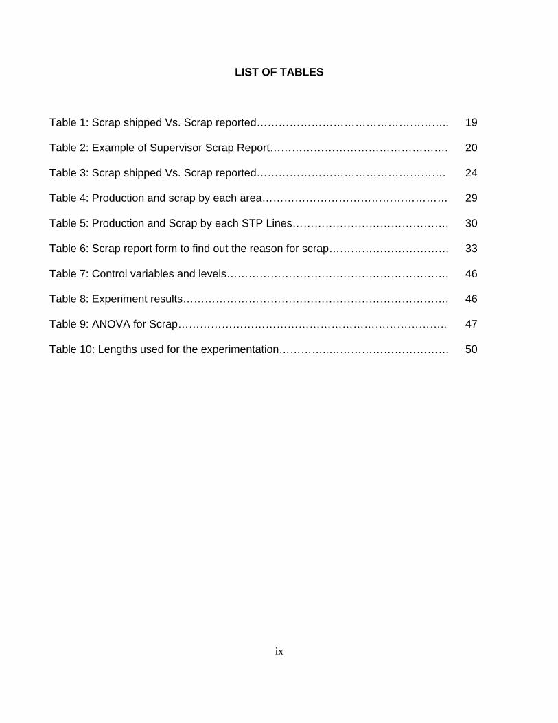
LIST OF TABLES
Table 1: Scrap shipped Vs. Scrap reported…………………………………………….. 19
Table 2: Example of Supervisor Scrap Report…………………………………………. 20
Table 3: Scrap shipped Vs. Scrap reported……………………………………………. 24
Table 4: Production and scrap by each area…………………………………………… 29
Table 5: Production and Scrap by each STP Lines……………………………………. 30
Table 6: Scrap report form to find out the reason for scrap…………………………… 33
Table 7: Control variables and levels……………………………………………………. 46
Table 8: Experiment results………………………………………………………………. 46
Table 9: ANOVA for Scrap……………………………………………………………….. 47
Table 10: Lengths used for the experimentation…………..…………………………… 50

x
LIST OF FIGURES
Figure 1: (a) Application of wires in Automotive Manufacturing Industry……………. 1
(b) Application of wires in Security and Home Technology………………... 1
(c) Application of wires in construction: industrial, commercial, residential 1
Figure 2: (a) Example of Insulated wire scrap………..…………………………………
(b) Example of Purge Scrap……………………………………………………
2
2
Figure 3: Comparison of Insulating scrap performance of all CCI manufacturing
………… units…………………………………………………………………..................
3
Figure 4: Approximation of what sigma variability looks like ……………….………… 6
Figure 5: (a) Example of Water Tree in XLPE wire……………………………………. 8
(b) Example of Water Tree in XLPE wire…………………………………….. 8
Figure 6: Process Flow chart of wire from copper to Insulation………………………. 12
Figure 7: Old Scrap Logistic……………………………………………………………… 22
Figure 8: New Scrap Logistic…………………………………………………………….. 23
Figure 9: Insulation Scrap Percentages ………………………………………………... 25
Figure 10: Silicone Scrap percentages………………………………………………….. 26
Figure 11: PCV Scrap percentages……………………………………………………… 27
Figure 12: XLPE Scrap percentages……………………………………………………. 28
Figure 13: Percentage of Scrap From total Scrap all areas…………………………... 29
Figure 14: Percentage of Scrap from total Scrap by all STP lines…………………… 31
Figure 15: Example of color change scrap by purging of compound through

xi
………… extruder …..………………………………………………………………....... 34
Figure 16: Example of Lump defect observed on the wire……………………………. 35
Figure 17: Example of spark out observed, mostly on small gage wire……………... 35
Figure 18: Example of Screen filter……………………………………………………… 37
Figure 19: Reason for scrap pareto……………………………………………………… 39
Figure 20: Color change process flow diagram………………………………………… 41
Figure 21: Main Effects Plot……………………………………………………………… 47
Figure 22: Interactions Plot for Scrap…………………………………………………… 48
Figure 23: Cube plot………………………………………………………………………. 49
Figure 24: Scrap results when color changed at 35000, 37500 and 40000 feet…… 51
Figure 25: PVC Scrap Percent YTD…………………………………………………….. 52
Figure 26: XLPE Scrap Percent YTD……………………………………………………. 54
Figure 27: El Paso Insulation scrap percentage 2010………………………………… 55
Figure 28: Box Plot Insulation scrap percentage May 2010 to November 2010……. 55
Figure 29: (a) Three axis gauge………………...……………………………………….. 58
(b) Two axis gauge……………..…………………………………………….. 58
Figure 30: Probability detection………………………………………………………….. 58
1
CHAPTER 1: INTRODUCTION
1.1 Background of Company
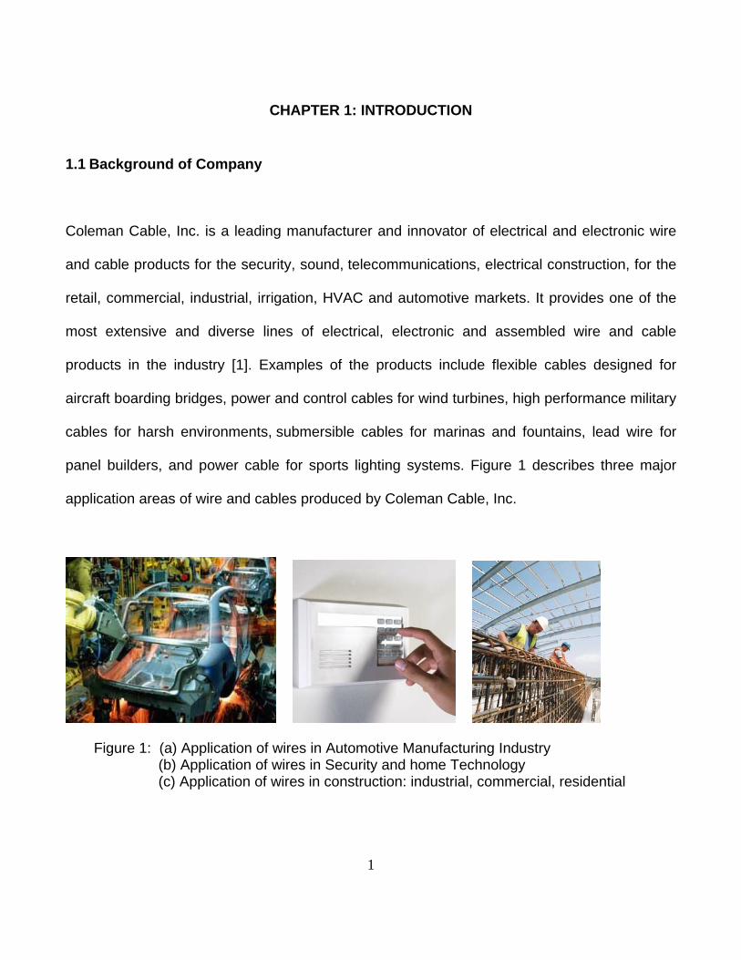
Coleman Cable, Inc. is a leading manufacturer and innovator of electrical and electronic wire
and cable products for the security, sound, telecommunications, electrical construction, for the
retail, commercial, industrial, irrigation, HVAC and automotive markets. It provides one of the
most extensive and diverse lines of electrical, electronic and assembled wire and cable
products in the industry [1]. Examples of the products include flexible cables designed for
aircraft boarding bridges, power and control cables for wind turbines, high performance military
cables for harsh environments, submersible cables for marinas and fountains, lead wire for
panel builders, and power cable for sports lighting systems. Figure 1 describes three major
application areas of wire and cables produced by Coleman Cable, Inc.
Figure 1: (a) Application of wires in Automotive Manufacturing Industry (b) Application of wires in Security and home Technology (c) Application of wires in construction: industrial, commercial, residential
2
1.2 Statement of Problem: Scrap and Scrap Reduction
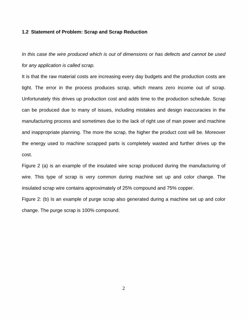
In this case the wire produced which is out of dimensions or has defects and cannot be used
for any application is called scrap.
It is that the raw material costs are increasing every day budgets and the production costs are
tight. The error in the process produces scrap, which means zero income out of scrap.
Unfortunately this drives up production cost and adds time to the production schedule. Scrap
can be produced due to many of issues, including mistakes and design inaccuracies in the
manufacturing process and sometimes due to the lack of right use of man power and machine
and inappropriate planning. The more the scrap, the higher the product cost will be. Moreover
the energy used to machine scrapped parts is completely wasted and further drives up the
cost.
Figure 2 (a) is an example of the insulated wire scrap produced during the manufacturing of
wire. This type of scrap is very common during machine set up and color change. The
insulated scrap wire contains approximately of 25% compound and 75% copper.
Figure 2: (b) Is an example of purge scrap also generated during a machine set up and color
change. The purge scrap is 100% compound.

3
Figure 2: (a) Example of insulated wire scrap Figure 2: (b) Example of purge scrap
0.00%
2.00%
4.00%
6.00%
8.00%
10.00%
12.00%
14.00%
January February March April May June
BremenMain
BremenEast
Lafayette El Paso
Insulating Scrap Performance Jan 2010 - June 2010
Figure 3: Comparison of insulating scrap performance of all CCI manufacturing units

4
There is critical need of scrap reduction in El Paso unit. Since the beginning of 2010, the El
Paso manufacturing unit has had more scrap than all the other manufacturing units. The scrap
numbers from January to May were incorrect as there was no system in place to report and
record scrap accurately. And the numbers showed in Figure 3 from the production record. The
major objective of the study is two. First, an accuracy reporting system for scrap is needed.
And second, strategies to reduce the production time, cost and significant scrap reduction are
required.

5
CHAPTER 2: LITERATURE REVIEW
This chapter describes and summarizes various strategies and the techniques that has been
applied and practiced to reduce scrap. Among them, Six Sigma Methodology is one of the
major techniques used in the practice to reduce scrap.
2.1 Six Sigma Methodology
Six Sigma is an approach towards quality assurance, quality management and continuous
quality improvement and its application can be wide including scrap reduction. The main
objective of using Six Sigma Methodology is to reach level of quality and reliability with low
scrap that will satisfy and even exceed demands and expectations of today’s demanding
customer of cable and wire for automotive industry [2].
A term “Sigma Quality Level” is used as an indicator of a process goodness. Lower sigma
quality level means greater possibility of defective products, while, higher sigma quality level
means smaller possibility of defective products within process [3, 4].
If Sigma quality level can be reduced to six, chances for defective products are 3.4 parts per
Million (ppm) [5, 6]. One ppm is 1 part in 1 million or the value is equivalent to the absolute
fractional amount multiplied by one million [7]. Tools and methodology within Six Sigma [8, 9]
deal with overall costs of quality, both tangible and intangible parts, trying to minimize it, while,
in the same time, increasing overall quality level contribute to profit [10].

6
Figure 4: Approximation of what sigma variability looks like [10]
Six Sigma means measure of quality that strives for near perfect product. It is a disciplined,
data-driven approach and methodology for eliminating defects (driving toward six standard
deviations between the mean and the nearest specification limit) in any process -- from
manufacturing to transactional and from product to service.
The statistical representation of Six Sigma describes quantitatively how a process is
performing. Application of Six Sigma can be on the process or product for reduction of
production cost, scrap reduction etc. The fundamental objective of the Six Sigma methodology
is the implementation of a measurement-based strategy that focuses on process improvement

7
and variation reduction through the application of Six Sigma improvement projects. This is
accomplished through the use of two Six Sigma sub-methodologies: DMAIC and DMADV. The
Six Sigma DMAIC processes (define, measure, analyze, improve and control) is an
improvement system for existing processes falling below specification and looking for
incremental improvement. The Six Sigma DMADV process (define, measure, analyze, design
and verify) is an improvement system used to develop new processes or products at Six
Sigma quality levels. It can also be employed if a current process requires more than just
incremental improvement [11].
Companies save an average of $100,000 to $200,000 per implemented improvement project,
for example, General Electric (GE) increased communication satellites’ usage from 63% to
97% realizing a revenue increase of $1.3 million/year. GE changed the original Motorola Six
Sigma model to a project based approach that had executive buy-in. GE saved $2 billion
during 1999. Companies that have produced good results, have invested adequate resources,
provided extensive training and involved many individuals [12].
2.2 Prevention of Water Tree
Water tree has always been an area of concern in making cables and wire. There are XLPE
(Cross Link Polymer) insulations that can be designed to inhibit the growth of water trees,
allowing for even greater reliability for distribution class cables.

8
Figure 5: (a) Example of water tree in XLPE wire; (b) Example of water tree in XLPE wire.
Water trees grow relatively slowly over a period of months or years. As they grow, the
electrical stress can increase to the point that an electrical tree is generated at the tip of the
water tree [14-16]. Once initiated, electrical trees grow rapidly until the insulation is weakened
to the point that it can no longer withstand the applied voltage and an electrical fault occurs at
the water/electrical tree location [13]. Then it becomes extremely difficult to stop water tree and
generates more and more scrap for every change. Many actions can be taken to reduce water
tree growth, and the approach that has been most widely adopted is the use of specially
engineered insulating materials designed to limit water tree growth. These insulation materials
are called WTR-XLPE (Water Cross Link Polymer). These insulation materials, combined with
the use of “clean” shields and suitable manufacturing processes have dispelled the concerns
that many utilities had regarding the use of cables with a polymeric insulation [13]. Two
approaches have been in widespread use to retard the growth of water trees and each is a

9
modification of the classic XLPE materials: Modification of the polymer structure, “Polymer”
WTRXLPE sometimes termed Copolymer - modified XLPE (Cross Link Polymer); modification
of the additive package, “additive” WTRXLPE; sometimes termed TR-XLPE.
In both instances, the compounds maintain the excellent electrical properties of XLPE high
dielectric strength and very low dielectric losses. WTR-XPLE insulations were commercialized
in the early 1980’s and have now been performing reliably in service for over 20 years [15, 17].
2.3 Improving Cleanliness and Smoothness for less defects
The critical importance of cleanliness (of both the insulation and the semiconducting screens)
and smoothness (insulation screen interface) has been a hard learned lesson [14, 16, 18 &
19]. It is also important because it causes contamination and the wire comes with lumps and
sparks. Improved cleanliness and interface smoothness increases operating stresses
(important for High voltage (HV) & extra high voltage (EHV)) and delivered life which is very
important for HV (High voltage cable) and EHV (Extra high voltage). Cleanliness and
smoothness of all cable materials has improved significantly over the last 15 years. In the
practice, production test has become an important strategy to assure that cables are good
quality and made according to required specifications. Cable manufacturers conduct these
tests before the cable leaves the factory. Most of the widely used cable standards [13, 14]
include production test procedures and requirements. However, it should be recognized that
these tests represent the minimum requirements. By improving the cleanliness during the
production helped the industry to reduce quality issues and it reflected on the number of
customer complaints.

10
Cleaner raw materials, improved manufacturing technology, and handling techniques have all
contributed to enhanced cleanliness. Out of these many initiatives including new generations
of XLPE and WTR-XLPE materials have emerged. These are generally supplied with
designations that define the cleanliness and voltage use levels.

11
CHAPTER 3: DMAIC (DEFINE PHASE)
This chapter explains the define phase of DMAIC approach and describes the manufacturing
processes of the wire, starting from the raw copper rod leading to the detail of copper thinning
and insulation. And also, explains the major and important aspects of making wire and about
the core wire manufacturing. The main objective of DMAIC was to identify areas in the process
where extra expenses exist, identify the biggest impact factor related with production
expenses, introduce appropriate measurement system, optimize process and reduce
production cost and time.
3.1. Define Phase
The main goal in define phase was to identify and decrease scrap. There were several major
causes for the high production expense variability in manufacturing wire. An adequate metrics
for evaluating projects success should be established.
When the project was started, very few useful historical data were available, so the first step
was to collect and select these data in the processes. In order to do this, all manufacturing
processes have been reviewed and studied in section 3.2 and 3.3.
3.2 Overview of Manufacturing Process
Figure 6 describes the series of manufacturing processes of wires. The starting material is
copper rod bought from the vendor, and then it goes to the rod mill. In rod mill, the wire is

12
thinned down into thinner copper wire then comes to the multi wire, where the copper wire is
annealed and drawn into the thinner and finer wire and all single strands is then took up into
the reels. The reels are then taken to the bunchers, in the bunchers proper lay is given to the
thin copper wire, according to the process guide requirement.
Copper Rod [17] Thinned Copper Multi wire
Insulated wire Bunched copper
Figure 6: process flow chart of wire from copper to Insulation
After bunching the wire, it goes to the extrusion line for insulation. According to the customer
requirements the operators get the required reel. This is the area where my research focused
because the goal was to reduce the scrap during insulation. This is considered to be very
critical as it requires precession and accuracy to get correct quality of wire as soon as
possible.
Rod Milling
Multi wiring
Bunching
Extrusion

13
3.3 Cable Manufacturing
Cable manufacturing is a multistep process. The conductor material (e.g., copper wire) is first
drawn to the specified diameter. The bare wire is then transferred to the wire coating line,
where electrical insulation material is extruded onto the conductor using a single-screw
extruder. The wire coating line typically consists of an unwinding roll for the wire followed by a
tension controlled input capstan, possibly a wire straightener, and a wire preheater, which
improves the adhesion of the plastic to the conductor. The wire proceeds from the preheater to
the extruder’s crosshead die, where the melted plastic insulation is applied. Processing
temperatures in the die average 400°F (204°C) for HDPE (High Density Polyethylene) and 650
to 700°F (343 – 371°C) for FEP (Fluorinated Ethylene Propylene). The coated wire continues
through a water bath and/or air-cooling system, spark tester, gauge controller, tension output
capstan, and tension controller, and is then wound onto a bobbin or reel. Output rates for
extruding the wire insulation average approximately 550 m/min (1,800 ft/min) for FEP and
1,500 m/min (5,000 ft/min). After the insulation has been applied, two conductors are twisted
together (paired) in a process called twinning. The number of twists per foot is precisely
controlled during the twinning process, and each of the four pairs is twisted differently (i.e.,
different number of twists per foot) in order to limit crosstalk between pairs in the final cable.
Twinning lines use two motors: one to feed insulated wire to the process and one to take up
the twisted conductor pairs. The next step is cabling, in which four of the twisted pairs are
bunched or stranded together with a cross-web separating the twisted pairs. A jacket, which
protects the conductors from mechanical damage and provides fire retardancy, is then
extruded over the core using a process similar to the one used to apply the wire insulation. Any

14
markings are printed onto the cable jacketing during this step. Jacketing proceeds at an
average speed of 400 to 500 feet per minute (120-150 m/min); temperatures in the die average
320 to 350°F (160 – 177°C). Both the CMR and CMP cables use compounded PVC for the
jacketing. The final cable product is tested for adherence to electrical parameters and then
packaged into customer-desired lengths. The primary wastes from the cable manufacturing
process (excluding waste from the copper drawing process) are scrap cable, and insulation
and jacketing resins. Any insulation or jacketing that is bled from the extruding lines during
start-up or shut-down is collected and recycled to the process. Pre-consumer PVC waste is
relatively easy for PVC compounders and cable extruders to recycle and reuse as an
equivalent for virgin PVC, because the composition is known.
3.3.1 Core Manufacturing
An extruded cable production line is a highly sophisticated manufacturing process that must be
run with great care to assure that the end product will perform reliably in service for many
years. It consists of many sub processes that must work in concert with each other. If any part
of the line fails to function properly, it can create problems that will lead to poorly made cable
and will potentially generate many meters of scrap cable [16].
Influence of Extrusion Head Configuration on Cable Aging, as measured by breakdown
strength [17], the process begins when pellets of insulating and semiconducting compounds
are melted within the extruder. The melt is pressurized and this conveys material to the
crosshead where the respective cable layers are formed [19].

15
Between the end of the screw and the start of the crosshead it is possible to place meshes or
screens, which act as filters. The purpose of these screens was, in the earliest days of cable
extrusion, to remove particles, or contaminants that might be present within the melt. While still
used today, the clean characteristics of today’s materials minimize the need for this type of
filter. In fact, if these screens are too tight, they themselves can generate contaminants in the
form of scorch or pre cross-linking. Nevertheless, appropriately sized (100 to 200-micron hole
size) filters are helpful to stabilize the melt and protect the cable from large foreign particles
that most often enter from the materials handling system. The most current technology uses a
method called a true triple extrusion process where the conductor shield, insulation and
insulation shield are coextruded simultaneously. The cables produced in this way have been
shown to have better longevity [17]. After the structure of the core is formed the cable is cross-
linked to impart the high temperature performance. When a CV tube is used fine control of the
temperature and residence time (lines peed) is required to ensure that the core is cross-linked
to the correct level [15].
3.3.2 XLPE Insulation
XLPE is a thermoset material produced by the compounding of LDPE with a crosslinking agent
such as dicumyl peroxide In this process, the long-chain PE molecules “crosslink” during a
curing (vulcanization) process to form a material that has electrical characteristics that are
similar to thermoplastic PE, but with better mechanical properties, particularly at high
temperatures. XLPE-insulated cables have a rated maximum conductor temperature of 90°C
and n emergency rating of up to 140°C.

16
• Insulation Curing Processes
The crosslinking process begins with a carefully manufactured base polymer. A stabilizing
package and crosslinking package are then added to the polymer in a controlled manner to
form the compound. Crosslinking adds tie points into the structure. Once cross-linked the
polymer chains retain flexibility but, cannot be completely separated. For example, they can be
transformed into a free-flowing melt. There are essentially two types of crosslinking processes
that can be used for XLPE-insulated power cables:
Peroxide cure – thermal decomposition of organic peroxide after extrusion initiates the
formation of crosslinks between the molten polymer chains in the curing tube. This process
can be used for XLPE or EPR insulations. The peroxide cure method is the most widely used
crosslinking technology globally and is used to manufacture MV (Medium voltage), HV (High
Voltage) and EHV (Extra High Voltage) insulated cables. The moisture-cure approach is
almost universally used for making LV cables and is sometimes used to manufacture MV
cables.
Moisture cure – chemical (silane) species are inserted onto the polymer chain; these species
form crosslinks when exposed to water. The curing process occurs in the solid phase, after
extrusion. Moisture curing is most often preferred for the manufacture of MV cables when
many different cable designs are made on the same extrusion line and/or when manufacturing
lengths are relatively short. In these situations, the separation of the extrusion and curing
processes is attractive from a production standpoint.
17
CHAPTER 4: DMAIC (MEASURMENT PHASE)
This chapter describes my first research task: scrap logistic which has been used to measure
scrap accurately from June 2010. The old scrap logistic and new scrap logistic will be
compared and discussed. The measurement by using the new scrap logistic will be described.
It has been approved that the new scrap logistic can measure the scrap accurately and
reduces material handling.
4.1 Scrap Logistic
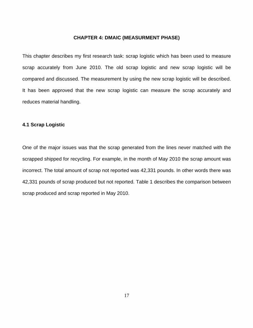
One of the major issues was that the scrap generated from the lines never matched with the
scrapped shipped for recycling. For example, in the month of May 2010 the scrap amount was
incorrect. The total amount of scrap not reported was 42,331 pounds. In other words there was
42,331 pounds of scrap produced but not reported. Table 1 describes the comparison between
scrap produced and scrap reported in May 2010.

18
Scrap generated during the month of May per Department.
Table 1: Scrap produced Vs. scrap reported
Total of scrap shipment shipped (6 shipments)
PVC ins
Battery Ln Bonder QA Towers Silicone
1st load (Lbs) 0 0 0 0 0 0 2nd load (Lbs) 35,001 6,095 1,175 3rd load (Lbs) 28,997 7,605 2,076 4th load (Lbs) 27,179 8,040 704 675 753 5th load (Lbs) 28,948 6,970 722 774 6th load (Lbs) 33,080 2,555 2,393 719 Total shipped (Lbs) 153,205 31,265 3,819 3,251 1,449 1,472 Total reported (Lbs) 120,844 28,024 1,462 0 0 1,800 Total not reported (Lbs) -32,361 -3,241 -2,357
-3,251 -1,449 328
The first target was to bring the scrap generated numbers equal to scrap shipped. A summary
of the daily scrap was recorded in a form. The daily scrap form was used by the supervisor to
verify the pounds of scrap generated, reported and shipped.

19
Table 2: Example of Supervisor Scrap Report
Shift Date: Supervisor
Box 1 Partial Box
Full Box
Difference Box 2 Scrap (Lbs)
Total Box
Total Shift Difference
Extruder Cu
Extruder Cu
Extruder TC
Extruder TC
Bare Cu
Bare Cu
Tin Cu Tin Cu Purge Purge
Extruder (Lbs) Bare (Lbs)
Purge scrap
Line # Operator Gauge Description
Copper Tin
Copper Tin (Lbs)
SCV 1 Total SCV 2 Total SCV 3 Total Total By Shift
The supervisor at the end of the shift collects the scrap summary form from all the production
lines and measures it. The supervisor is responsible if the scrap produced does not match the

20
scrap shipped. But there was still a difference between the shipped and the reported scrap.
The logistic of scrap travel was changed and different scrap boxes for night and day shift were
allotted. Even this didn’t help. Therefore, the time a supervisor spends in collecting scrap from
the lines which was approximately 2 hours every shift was noted. The scrap collection time
was presented before management. The time supervisor spends in scrap collection and entry
can be saved for better things. The operator should be responsible for the scrap generated on
the machine. This gave the supervisors the opportunity to assist operators on the line,
especially newly trained operators. After the change in scrap logistics, the total scrap
produced matched the scrap shipped and the production scrap was in control.

21
Old Scrap Logistic:-
START
Lead Operator logs in the weight of scrap drums in supervisor scrap login sheet
Operator puts the Purge scrap in the 22“purge drum
Operators put the insulated scrap wire in the 22” scrap drum
Lead sticks the Gaylord scrap form on Scrap Box
Lead Operator records the scrap information from the supervisors scrap form to the production report
Production report goes into the data base with scrap information
Log in the Scrap weight for all reasons in scrap form
Log in the Scrap weight for all reasons in scrap form
Lead Operator logs in the weight of scrap drums in supervisor scrap login sheet
Lead sticks the Gaylord scrap form on Scrap Box
Lead Operator weights the scrap box and places in the scrap area
Insulating Purge
Empties the scrap drum into the scrap Box from every line and at the end of the shift or whenever the online
Empties the scrap drum into the scrap Box from every line and at the end of the shift or whenever the online scrap drum is full.
Lead Operator weights the scrap box and places in the scrap area
Figure 7: Old Scrap Logistic

22
New Changed Scrap Logistic:-
Machine STP 1
Scrap Drums on the line
Purge Scrap Drum
Insulated Scrap Drum
Big Scrap Box for purge of capacity 1600 lbs
Big Scrap Box for insulated wire of capacity 1600 Lbs
These Scrap boxes have capacity of 1600 Lbs. In one shift approximately operator makes 200 to 250 lbs of scrap so the box will be full in 6 shifts which are 2 days.
Scrap shipping area
Figure 8: New Scrap Logistic

23
Table above shows that in the month of June the scrap reported was accurate as the scrap
shipped. This means that the improved scrap logistic worked.
Table 3: Scrap shipped Vs. Scrap reported
Total of scrap shipment shipped (5 shpments)
Loads /
ship date
PVC ins
Battery Ln
Bonder QA Towers Silicone Purge BC
Fab
BC
Ext
TC
UnIn
1st load
(Lbs) 2,132 0 0 0 0 0 34369
2nd load
(Lbs) 34,125 5,578 0 0 782 575
3rd load
(Lbs) 21,540 4,656 0 0 499 0
4th load
(Lbs) 25,269 2,940 1506 0 640 1173 6611 2426 1388
5th load
(Lbs) 0 0 0 0 0 0
6th load
(Lbs) 13,372
7th load
(Lbs) 17,737 3,360 2996 4733
Total shipped
(Lbs) 114,175 16,534 1,506 0 1,921 1,748 34,369 9,607 7,159 1,388
Total reported
(Lbs) 114,170 19,726 590 0 877 1,197 29,139 476
Total not reported
(Lbs) 0 3,192 -916 0 -1,044 -551 -5,230 -
9,607 -7,159 -912

24
4.2 Percentage of Scrap before June 2010
The scrap and production numbers for 2010 were provided along with the goal of 5% by the
end of December 2010. In order to determine the best targeted area to reduce the amount of
scrap. The Pareto was done for all insulating areas. The result of the Pareto determined the
best area of concentration.
• Total insulation scrap
Scrap % Total Insulation
5.63
7.939.23 9.31
10.1111.74
0.00
2.00
4.00
6.00
8.00
10.00
12.00
14.00
January February March April May June
Jan to May are not the true numbers
Figure 9: Insulation Scrap Percentages
In the graph it is clear that at the beginning of the year the company started well with
approximately 5% and from there it began to rise, reaching 11.74% in June. Since the
production was increasing it was not something unexpected but with the increase in production

25
no one concentrated on the scrap and this result in an increase of the scrap to 11.74% in June.
This factor alone clarifies the importance of this project.
• Silicone scrap
Total Scrap % Silicone
1.600.90
2.10 2.201.70
1.30
0.00
4.00
8.00
12.00
January February March April May June
Figure 10: Silicone Scrap percentages
It is clear (figure 10) that the silicone area was not the area of concern as the scrap from this
area was quite low. Silicone did not really have a major contribution to scrap, it was usually
below 2%.

26
• PVC scrap
Total scrap % PVC
5.47% 5.09% 5.09% 5.10% 4.76%
22.99%
0.00%
5.00%
10.00%
15.00%
20.00%
25.00%
January February March April May June
January to May are not the true numbers
Figure 11: PCV scrap percentages
There was a drastic change in the PVC scrap in the month of June. But before June as
explained in the previous chapter, the scrap reported was incorrect so even though the graph
says 5% it does not necessarily mean it was 5%. At this point it is impossible to determine the
correct percentage of scrap for the months prior to June. Since the supervisor scrap report
form has been adopted, the real numbers show the correct amount of scrap was 22.99%. The
correct reporting of scrap began in June. After this point the scrap has been calculated
accurately.
• XLPE Scrap

27
Total Scrap % XLPE
0.00%
2.00%
4.00%
6.00%
8.00%
10.00%
January February March April May June
Jan to May are not the true numbers
Figure 12: XLPE scrap percentages
The scrap for XLPE before June was definitely high than what is shown in Figure 12.
4.3 Concentrated Area
The Pareto analysis was done to determine which area produces a larger amount of scrap
when compared to other areas. It was determined that the larger percentage of scrap comes
from PVC as compared to other areas. The reason being that, the production pounds for PVC
are much higher than other areas.
Table 4: Production and scrap by each area

28
June 2010 Report on Production and Scrap
Production (Lbs)
Insulated Scrap (Lbs)
Purge Scrap (Lbs)
Total Scrap (Lbs)
% of scrap from total scrap
% of scrap STP lines
PVC 1705973.40 364151.00 28117.00 392268.00 87.58% 22.99% XLPE 475013.10 35182.00 5096.00 40278.00 8.99% 8.48% Silicone 158439.10 1642.00 16.00 1658.00 0.37% 1.05% Battery 230739.40 10863.00 2817.00 13680.00 3.05% 5.93% Total 2570165 411838 36046 447884 17.43%
PVC production was much higher than the XLPE, silicone and battery. Therefore, even the
scrap percentage was higher than other areas. The percentage of scrap it had from total
insulated scrap was also quite high of 87.58%.
0.00%
10.00%
20.00%
30.00%
40.00%
50.00%
60.00%
70.00%
80.00%
90.00%
100.00%
PVC XLPE Silicone Battery
% of scrapfrom totalscrap
% of scrapSTP lines
Figure 13: Percentage of Scrap From total Scrap all areas

29
The blue color bar represents the scrap percentages of the total insulated wire scrap. On the
other hand the maroon bar represents the area scrap percentages. The graph above (figure
13), shows that 87.58% of the scrap was produced from PVC, so it was clear that PVC area
needed to be the area of highest concentration.
• PVC Pareto
There are a total of five PVC lines. The Pareto analysis was done on all the PVC line to
determine the highest percentage contributor to scrap.
Table 5: Production and Scrap by each STP Lines
June 2010 STP Lines Production and scrap
Production Lines
Production (Lbs)
Insulated Scrap (Lbs)
Purge Scrap (Lbs)
total scrap % of scrap from total Scrap
% of scrap STP lines
STP 1 292414.60 74289.00 6501.00 80790.00 20.60% 27.63% STP 2 575641.80 72490.00 6081.00 78571.00 20.03% 13.65% STP 4 201794.80 72494.00 4501.00 76995.00 19.63% 38.16% STP 5 261963.40 102300.00 5610.00 107910.00 27.51% 41.19% STP 6 374158.80 42578.00 5424.00 48002.00 12.24% 12.83% Total 1705973.4 364151 28117 392268 22.99%

30
0.00%
5.00%
10.00%
15.00%
20.00%
25.00%
30.00%
35.00%
40.00%
45.00%
STP 1 STP 2 STP 4 STP 5 STP 6
% ofscrapfrom totalscrap
% ofscrapSTPlines
Figure 14: Percentage of Scrap from total Scrap by all STP lines
The above chart (figure 14), clearly indicates that all lines almost equally contribute to total
scrap except STP 6. The scrap percentage for all lines was quite high. After reaching the
results of scrap production for each line, the goal was to begin the reduction line by line. Since
STP 5 produced the greatest amount of scrap the goal was to reduce its scrap first, as it
makes heaviest wire than other lines.

31
CHAPTER 5: DMAIC (ANALYSIS)
This chapter describes the types of defects that occur on the wire during manufacturing
processes. And also, it explains how the scrap report form helps determine which type of
defect produces the most scrap, via the Pareto analysis.
5.1 Reason for Scrap
The percentage of scrap was increasing, and it was necessary to determine the reason behind
this. In order to measure scrap on a daily basis, samples were collected for inspection in the
laboratory under specialized equipment. Every defect indicates a problem with the machinery,
an operational problem or a processing issue. The major defects were analyzed using the 5
why analysis followed by knowledge obtained from the six sigma theory. It was difficult to
determine the major defects, as every machine operator has their own way of doing things.
Therefore, generated a table in which they would record the amount of scrap and the reason
for its existence. Generating this table was very helpful when it came time to inform the
engineers of the problems and issues found at hand. Prior to the use of this table operators did
not inform maintenance of any such issues until the production line had stopped completely
therefore the downtime was longer.

32
Table 6: Scrap report form to find out the reason for scrap.
Scrap report form PVC and CV Operator:
Date:
Line:
Gauge No.
Down time Color change
Purge scrap (Lbs)
Wire Scrap (Lbs)
Reason for scrap Stop time Start time
Number of color changes = Note: Write down the down time. Every time the machine stops due to any reason wire break, purge, gauge set up, maintenance etc. write down the time it stopped and then the time when again started manufacturing wire. Give reason for the scrap generated eg. lumps, OD defect, wire breaks, spark outs, color change etc. Be accurate in measuring the scrap. Do not forget to subtract the weight of drum from the measured purge and wire scrap. Comments:-
*Reference Only*
There can be many types of defects that can occur during the cable manufacturing process,
such as color change, lump, weld, air bubble, cold compound, outer diameter variation, center,
bleed over, spark outs etc.
• Color Change
This is the most common type of defect and cannot be avoided. But nothing was ever tried or
experimented to reduce color change scrap. This definitely needed to be reduced. The
numbers indicate that the scrap percentage would be lower if there were only a few color

33
changes. As the number of color changes increases the scrap percentage also increases. The
target was to reduce the pounds of scrap for every color change. There are two methods in
which color can be changed.
• Color change on the run
During this there should not be any change in the gauge. The machine continues running and
on the run the next color is added. But the downside of this process is that the color does not
change instantly. For example if it is changing from white to black. The wire will first change to
light grey then dark grey and then finally black. The change is gradual. This process produces
approximately of 30 pounds of insulated scrap. The good thing about this type of color change
is that is reduces downtime.
• Color change by purging the color compound
In this the entire compounds in the extruder has to be purged out. What exactly they do is take
out the tip and dye from the head and purge the entire compound present in the extruder. A
typical extruder can hold 43 pounds of compound. After purging entire compound from the
extruder the machine is started again. The wire produced after this kind of color change has
many defects and it takes a while to get good quality wire. But this process produces less
scrap than the scrap produced by doing a color change on the run.
Figure 15: Example of color change scrap by purging of compound through extruder

34
• Lump and neck
Lump and necks are created when the compound is not mixed well in the extruder and the
compound is still not heated properly. There are screen packs fitted just before the head to
catch all the unwanted particles and for the very small micro granules of compound. If the
screen packs are not changed in a timely manner the chances of getting lump and necks are
increased. There is a lump and neck detector on the line to detect if the wire has any lump or
neck. A typical lump defect on the wire is shown below (figure 16).
Figure 16: Example of Lump defect observed on the wire [20]
Figure 17: Example of spark out observed, mostly on small gauge wire

35
• Spark Outs
This happen when there is insulation missing on the wire. It could happen if the screen packs
are not changed in a timely manner. The screen packs gets clogged by the compound and the
small unwanted particles. Sooner or later come these particles come out with the wire and
sparks. Sparker are installed on the line to catch spark outs [21].
For both the above defects it was found that screen packs should be in good condition all the
times. Most of the extrusion processes pass melt through wire mesh screens on the way to the
dye to provide filtering and improved mixing. But screens also introduce process variables,
raising backpressure and melt temperature and sometimes reducing output. Screens are held
by a breaker plate with holes or slots, which form the seals between the extruder and dye.
Clean screens add only a small amount of pressure, maybe 50 to 100 psi, to the resistance of
the head. The greatest pressure variable is the amount of contamination they trap [21].
When clogged screens are changed, pressure suddenly drops, melt temperature may do the
same, and either screw rpm or line speed must be adjusted to maintain the same product
dimensions. When extruding a circular product, these process changes may not cause serious
problems, but in a flat or irregular profile shape, the melt temperature change may affect the
product shape. For instance, in a flat die, cooler melt will give sheet a thinner center and
thicker edges. This may be compensated for by automatically or manually adjustments to the
dye, but it shouldn’t be ignored. Placing a gear pump after the screen changer can prevent this
problem by maintaining constant output through the die. But the change in melt temperature
after a screen change may still require dye adjustments. Also, gear pumps have a very small

36
clearance that can be damaged by hard contaminants, so fine screens are needed to shield
the pump. Extruders of rigid PVC, for example, know that screens make the melt hotter, which
therefore needs more stabilization, which adds to material costs. Some suppliers offer special
screen changers for plasticized PVC. But for rigid PVC most processors either avoid screens
altogether, or use a relatively coarse pack without a changer to keep out only large
contaminant particles.
Figure 18: Example of screen filter [21]
Screens filter contamination and improved mixing, may raise pressure and temperature, which
can affect output and product dimensions [21].
• Weld
The copper wires for insulation are in reels. So in order to continue running without breaks we
have pay offs where we can weld the two wires. But the welded wire is not acceptable to the
customer so we have to scrap this wire as well. On the positive side the scrap produced by
weld is not very much and therefore not really given much focus.
• Air bubble

37
This type of defect is very common but can be very easily fixed. There needs to be a vacuum
given to the head from behind in order to suck all the air gaps. If the vacuum pump is not in
proper working condition we can have air bubble.
• Cold compound
This was a major issue with all the lines. They used to get cold compound wires during the
start ups. The reason being that when the operators purge the extruder for a color change the
temperature drops down as they slow down the line speed. So the temperature was not
sufficient to keep the compound heated enough. When they started producing the wire the wire
did not have a smooth surface. This was due to cold compound.
• Outer diameter variation
After purging the wire does not come out right according to the settings on the machine. It
needs to be adjusted slowly so that the correct OD (Outer Diameter) is obtained. So here it is
kept as low as possible. By the time correct OD is obtained the wire produced is all scrap. This
is the most important problem the company is dealing with.
• Center
Often when the operator purges the extruder, the center is lost which means the copper is not
at the center of the insulation. One of the reasons this may occur is due to the usage of worn
out tools. Even the pulleys located at the back of the head causes this problem. The pulley
needs to be adjusted every time there is a change in the gauge.

38
5.2 Reason for Scrap Pareto
0.00%
10.00%
20.00%
30.00%
40.00%
50.00%
60.00%
70.00%C
olo
rC
ha
ng
e
Lu
mp
We
ld
Air
Bu
bb
le
Ou
ter
Dia
me
ter
Ce
nte
r
Sp
ark
Hig
hS
tra
nd
Wir
eB
rea
k
STP 1
STP 5
STP 6
Figure 19: Reason for scrap pareto
The graph above shows that for STP 1, 5 & 6 color change has been the major concern. Even
though the color change scrap cannot be eliminated, it can definitely be reduced significantly.
Types of Defect

39
CHAPTER 6: DMAIC (IMPROVE)
This chapter briefly explains the flow of the color change process, and the critical operations
and factors involved in this process. Furthermore, the different scrap approaches of reducing
scrap have been discussed and compared.
6.1 Background of Color Change Process Flow
One of the objectives of project was to identify major process variables impacting the high
expenses. The Pareto chart for total expenses, in the measurement phase in Chapter 5 is
displays that PVC would give a major impact for scrap reduction. Based on Pareto chart, the
decision was made to analyze and make improvements within the working style of operator.
The change in some method and fixing of some machine issues would bring it to direct half of
what it was in June 2010. There was also acquiesced that quality improvement and reduction
of quality costs within process are achievable. The significant improvement in scrap could be
accomplished by: 1) reduction of cycle time, 2) reduction of control time, 3) reduction of down
time.
From the PVC scrap by color change was chosen because Pareto diagram showed that it is
major contributor to scrap. The chosen color change process involves the following steps.

40
The process map was drawn for all operations in the color change and a list of the input and
output variables were completed. The input variables were ranked as, Critical, Noise,
Controllable and Standard operating procedures variable and, furthermore, non-value added
operations are defined and marked. Scrap from color change was always going to be there but
can be reduced for sure. Only lowering down number of color changes was not going to help.
Every time color change is done approximately 50 pounds of scrap is produced.
Finding right compound and color chip
Getting right color from extruder
Machine start up for purge
Stopping the machine
Cleaning the head
Getting right center, color, OD, wall
thickness, strip force
Starting the machine
Figure 20: Color change process flow diagram

41
The most critical operations were the amount of compound and color chip added to the
extruder and the time when to stop the machine. Conducted analysis showed that there was
no data or value for when to change the color in other words when to stop pouring more
compound. The extruders keeps filling all the time through the vacuum and sensor control as
soon as it senses that there is no compound the vacuum starts and extracts compound.
6.2 Approach to Reduce Scrap
As the main goal was to identify and decrease scrap in process by 5% [22]. The objective was
to determine a specific value at which the pouring of the compound into the extruder should
cease at the end of the work order. During the analysis few detail things were fined like
capacity of the extruder, time taken for the extruder to purge out the compound at a certain
speed and what the operator does during the purging of compound. The extruder was
completely filled. After the extruder was completely filled the no more compound was given to
the extruder for that particular order. To stop pouring compound the operator has climb the
ladder all the way to the hopper to switch off the machine. At a temperature of 355°F all zones
had the same speed of 300 fpm. At this speed it took 15 minutes for the extruder to purge its
contents completely.
The extruder can hold up to 62 pounds of compound. So every time they change the color of
the wire they have approximately 62 pounds of purge scrap. At this point calculated the
amount of compound needed to produce insulated wires of different gauges. In this case of
approximately 42 pound of compound was needed to make certain feet for wire. Therefore

42
operator was given 62 pounds of compound and 2 pounds of colored chips in order to produce
the work order.
The production line started, but until the operator could produce a high quality wire, 20 pounds
of insulated wire was already scraped. However, the contents of the extruder, was still enough
to produce required wire to full fill the work order.
Even though the calculations were correctly determined and only 42 pounds of compound was
required, the outer diameter decreased at the end of the work order due to a lack of pressure
in the extruder, produced by the compound. The decrease in pressure resulted in a smaller
amount of compound being excreted from the head of the extruder. As a result increasing the
outer diameter setting on the extruder did not help. Therefore the work order was not
competed, and resulted in the work order being short.
In this approach, 62 pounds of compound was poured into the extruder. But at the same time
even after filling up the extruder the vacuum pump for supplying the compound to the extruder
was not stopped. During this experiment the color change was from white to black. Started
producing white wire and towards the end of the work order the color was changed to black
using black chips. This would allow for continuous production of wire without ceasing
production. But the downside would be that the color does not change immediately, it would
fade into black.

43
So either stop running the extruder and purge the contents or continue running the extruder
but in this case the amount of scrap would increase and would contain copper. Being that
copper is quite expensive, the decision to stop the extruder and obtain the quality of black
desired was made. In doing so, scrap was reduced and 10 pounds of copper and compound
were saved.
The next step was to determine the appropriate time to change the color. In order to do so,
experiment was designed to determine the value and length when the color needs to be
changed to get least amount of scrap.
According to the capacity of the extruder for every gauge the amount of compound required to
manufacture the length of wire needed was calculated. For a 2.0 gauge wire the extruder
required 37.26 pounds of compound to produce 40,000 feet or wire. Once the extruder has
produced 35,000 feet of wire it still has enough compounds to produce another 5,000 feet or
wire. Therefore, color can be changed at this point and by doing so we 4,000 feet of wire and
20 pounds of compound can be saved.

44
CHAPTER 7: STATISTICAL ANALYSIS: DESIGN OF EXPERIMENTS AND RESULTS
This chapter describes the two step statistical analysis. First a full factorial design is
implemented with a few factors, such as length, speed and temperature. Results from main
effects, two factor interaction and three way interaction are discussed and significant factors
are identified. Finally this continues with the optimum level of factors obtained to produce the
least amount of scrap.
7.1 Statistical Analysis
The design of experiments involves three controllable variables (settings) length, speed and
temperature. Table 7 shows the variables with their low and high levels.
A 23 (three factors and two levels) was used. It is a full factorial design. Matrix and data for
scrap is shown in Table 7. The software used for the analysis is Minitab 16.
Step 1
Control Variable and their levels:
Control variable is that factor which is controlled by the experimenter to cancel out or
neutralize any effect they might otherwise have on the observed phenomenon (dependent
variable). The control Variables used in this experimentation were, Length, Speed and
Temperature as shown in Table 7.

45
Table 7: Control variables and levels
Control Variable Low Level High Level
Length (ft) 35000 40000
Speed (ft/min) 1000 1500
Temperature (ºF) 325 350
Table 8: Experiment results
Run
Number
Length (ft)
Speed (ft/min)
Temperature (ºF)
Scrap (lbs)
Run 1 35,000 1,500 350 21 Run 2 40,000 1,500 350 45 Run 3 35,000 1,000 325 25 Run 4 40,000 1,000 350 55 Run 5 35,000 1,000 325 28 Run 6 35,000 1,500 350 22 Run 7 40,000 1,500 350 56 Run 8 35,000 1,500 325 25 Run 9 40,000 1,500 325 46 Run 10 35,000 1,500 325 23 Run 11 40,000 1,000 325 58 Run 12 35,000 1,000 350 26 Run 13 40,000 1,000 325 56 Run 14 40,000 1,000 350 57 Run 15 35,000 1,000 350 24 Run 16 40,000 1,500 325 59

46
Table 9: ANOVA for Scrap
Estimated Effects and Coefficients for Scrap (Lbs) (coded units) Term Effect Coef SE Coef T P Constant 39.125 1.111 35.22 0.000 Length 29.750 14.875 1.111 13.39 0.000 Speed -4.000 -2.000 1.111 -1.80 0.110 Temperature -1.750 -0.875 1.111 -0.79 0.454 Length*Speed -1.000 -0.500 1.111 -0.45 0.665 Length*Temperature 0.250 0.125 1.111 0.11 0.913 Speed*Temperature -0.500 -0.250 1.111 -0.23 0.828 Length*Speed*Temperature -0.000 -0.000 1.111 -0.00 1.000 S = 4.44410 PRESS = 632
R-Sq = 95.82% R-Sq(pred) = 83.28% R-Sq(adj) = 92.16%
• Main Effects
4000035000
50
40
30
2015001000
350325
50
40
30
20
Length
Mea
n
Speed
Temperature
Main Effects Plot for Scrap (Lbs)Data Means
Figure 21: Main Effects Plot

47
A main effect is an outcome that is a consistent difference between levels of a factor. The main
effects plot is used to examine the main effects of factors. The main effects of three setting
length, speed and temperature are shown in main effect plot (figure 21). It can be observed
that length has a significant effect on the scrap. Speed and temperature has no significant
effect on scrap. Also at 35,000 feet scrap is less than what it was at 40,000 feet.
• Two-factor Interactions
15001000 35032560
40
2060
40
20
Length
Speed
T emperature
3500040000
Length
10001500
Speed
Interaction Plot for Scrap (Lbs)Data Means
Figure 22: Interactions Plot for Scrap
Figure 22, shows the two factor interaction plot, information for all possible two factor
interactions that should be examined [23]. And was found that length speed interaction is not
significant and length temperature is not significant either. The same conclusion can be drawn
from (ANOVA Table 9).

48
• Three Factor interactions
350
325
1500
10004000035000
Temperature
Speed
Length
50.5
56.025.0
21.5
52.5
57.026.5
24.0
Cube Plot (data means) for Scrap (Lbs)
Figure 23: Cube plot
From the cube plot (Figure 23), it is found that the least scrap can be achieved at low length
(35000 ft), high speed (1500 ft/min) and high temperature (350 ºF).

49
Step 2
Set of Experiments:
Table 10: Lengths used for the experimentation
Set of Experiments
Length (ft)
1 35,000 2 35,000 3 35,000 4 35,000 1 37,500 2 37,500 3 37,500 4 37,500 1 40,000 2 40,000 3 40,000 4 40,000
Using the temperature, speed, outer diameter, and other settings mentioned in the process
guide, the finds were consistent for the three lengths and the 4th trial was done for every
length.

50
Scrap
0
10
20
30
40
50
60
70
1 2 3 4 5 6 7 8 9 10 11 12
Scrap
1st Set of Experiment Length 35000 everytime
3rd Set of Experiment Length 40000 everytime
2nd Set of Experiment Length 37500 everytime
Length ft
Scrap Lbs
Figure 24: Scrap results when color changed at 35,000, 37,500 and 40,000 feet
The above graph shows that with one length, 4 trials were performed and scrap readings were
taken. The result is shown in the graph above (figure 24). For the length of 35,000 feet the
scrap was close to 20 pounds. For 37,500 feet the scrap was approximately 50 pounds and for
40,000 feet was as expected, 60 pounds.
The graph proves that the length 35,000 feet will produce the lowest amount of scrap, from 20
pounds to 25 pounds. By using this length almost 40 pounds of compound was saved at every
color change for 2.0 gauges. Like this for 3.0, 5.0, 1.25 and 0.85 lengths were found when the
color should be changed to get the least amount of scrap.

51
7.2 Results and Discussions
• Year To Date Total PVC Scrap percentage
With the scrap reduction the production cost also was successfully reduced with process
organization [24]. The scrap percentage of PVC for the month of June 2010 was 22.99% and
for November was 7.6% which means there was a reduction of 15.39%. Every month saw a
consistent decrease in scrap percentage.
0.00%
5.00%
10.00%
15.00%
20.00%
25.00%
Janu
ary
Febr
uary
Mar
ch
Apr
il
May
June
July
Aug
ust
Sep
tem
ber
Oct
ober
Nov
embe
r
Dec
embe
r
PVC Scrap % YTD Jan to May are not true numbers
Project Experimentation starts
Figure 25: PVC Scrap Percent YTD
June 2010 saw major jump in scrap in PVC lines which contributed to the total insulation scrap.
Reporting of right scrap started in the month of June 2010 and that’s when company came to

52
know the correct percentage of scrap. Before June the percentage shown in the graphs are the
one on the production reports but the amount of scrap shipped and amount of scrap reported
were not even close. Another reason why June was high is because the company
concentration in June was more on Quality.
The scrap for October and November could not go down because of high number of color
changes. As explained before the scrap from color change cannot be avoided. And is one of
the major reasons why the scrap percentage did not decrease that much. The numbers of
color changes for May on PVC lines and for the October were compared. For example STP 1
did 86 color changes in 10 days in comparison to 181 color changes in October 2010.

53
• Year To Date Total XLPE Scrap 2010
Scrap project on XLPE started in August 2010. In August 2010 the scrap percentage was
15.14% and in November 2010 it was 7.2% which means there was decrease of 7.94%
0.00%
5.00%
10.00%
15.00%
20.00%
Janu
ary
Febr
uary
Mar
ch
April
May
June
July
Augu
st
Sept
embe
r
Oct
ober
Nov
embe
r
Dec
embe
r
XLPE Scrap % YTD
Jan to May thenumbers are not right
Project Experimentation starts
Figure 26: XLPE Scrap Percent YTD
The scrap numbers from January to May are not the right numbers. But after the project
started on XLPE the scrap decreased.

54
• Total Insulation Result
Scrap % Total Insulation
0.002.004.006.008.00
10.0012.0014.00
Janu
ary
Febr
uary
Mar
ch
April
May
June July
Augu
st
Sept
embe
r
Oct
ober
Nove
mbe
r
Jan to May are not the true numbers
Figure 27: El Paso Insulation scrap percentage 2010
NovemberOctoberSeptemberAugustJulyJuneMay
17.5
15.0
12.5
10.0
7.5
5.0
Data
7.0147.38897
8.67797 8.89389
7.65355
6.00795.46677
Boxplot of May- November Insulation Scrap %
Figure 28: Box Plot Insulation Scrap percentage May 2010 to November 2010

55
The box plot (figure 28), shows a box encased by two outer lines known as whiskers. The box
represents the middle 50% of the data sample - half of all cases are contained within it. The
remaining 50% of the sample is contained within the areas between the box and the whiskers.
The single line in the box represents the median, which is middle value of entire sample. In this
case for November it is 5.4 %. You can see the scrap tendency and variation per month. It can
be observed that in November there was less variation.
• DMAIC (Control Phase)
This is the last phase of DMAIC methodology. In this control phase of DMAIC methodology, a
control plan will be developed to ensure that processes and product consistently meets
company and customer requirements, and to check how length still impacts on quality
production level [26, 27, and 28]. In this phase, large emphasis will be given on proper
implementation of solutions. For this, regular checking of check charts will be carried out.
Monitoring of scrap will be done shift wise, day wise and month-wise. The improvements will
be adhered to by providing training to the staff, implementing various incentives schemes and
adhering to the modified systems [25].

56
CHAPTER 8: CONCLUSIONS AND FUTURE DIRECTION
Conclusion:
Six Sigma methodology and Design of Experiments were used to reduce scrap. The
introduction of six sigma technologies to reduce scrap provided the company with new tool of
cost reduction. For this particular cost reduction project scrap improvement became the most
important source. The results suggested that the scrap came almost to half from where it was
in the beginning. Scrap percentage for total insulation area was 11.74% in May 2010 and
in November 2010 it was 5.38%. So Six Sigma with the help of DOE does help to determine
the correct setting for all the process and in that case for reduction of scrap too. Three factor
two level full factorial designs helped determine the significant factor to reduce scrap. The
analyses results showed that the scrap process was in control as compared to that before
November.
Future direction:
Defects generally result from a process problem or material contamination, which result in
lumps, breaks and neck-downs. The system Alarms and Reports Surface Quality Defects
(SQD) as they happen, using advanced 3-Axis Visible LED Detection technology to cover the
circumference of the product 3 times more effectively than 2-axis gauges. The one used in the
company is 2 axis gauges which mean if the defect is very small it might escape. 3 axis
gauges cover more area of the wire and will catch even smaller defects [29].

57
Figure 29: a) Three axis gauge b) Two axis gauge
Figure 30: Probability detection [29]
This approach shown in the figure 29 a) and b) is being considered by the company. In the
near future this process will be used to detect the defects more easily. The figure shows that
the probability of detection of defects is greater on 3 axis gauges than that of the 2 axis gauges
[29].

58
REFERENCES [1] www.colemancable.com.
[2] T. Pyzdek, The Six Sigma Revolution, Quality America Inc. 1999.
[3] M. Harry and R. Schroeder, Six Sigma: The Breakthrough Management Strategy
Revolutionizing the World’s Top Corporations, Currency, New York, 2000.
[4] F.W. Breyfogle III, Implementing Six Sigma: Smarter Solutions Using Statistical Methods,
John Wiley & Sons, Inc., New York, 1999.
[5] F. Cus, Produktionsmanagement in kleinen und mittleren Unternehmen. E I, Elektrotech.
Inf. Tech., 114 No. 4 (1997) 176-181.
[6] M. Sokovic, D. Pavletic, PDCA cycle vs. DMAIC and DFSS, Proceedings of the 1st
International Conference ICQME 2006, 13th-15th September, 2006, Budva, Montenegro.
[7] Z. Satterfield, What does ppm or ppb means? On tap fall, West Virginia, 2004
[8] T. Pyzdek, Six Sigma Implementation, John Wiley & Sons, Inc.,New York, 1999.
[9] R. Basu, Implementing Quality – A Practical Guide to Tools and Techniques, Thomson
Learning, London, 2004.
[10] www.operational-excellence.net.
[11] www.isixsigma.com.
[12] N. Dedhia, Six Sigma Basics, San Jose, 2005.
[13] N. Hampton, R. Hartlein, H. Lennartsson, H. Orton, R, Ramchandran, Long-Life XLPE
Insulated Power Cable, Jicable, 2007.
[14] H, Orton and R. Hartlein, “Long Life XLPE Insulated Power Cables”, October 2006.

59
[15] A. Campus and M. Ulrich, 20 Years Experience with Copolymer Power Cable Insulation.
Jicable03, Paper B1.6, 2003.
[16] L Dissado and J Fothergill, Electrical Degradation and Breakdown in Polymers; IEE
Materials and Devices, 1992.
[17] H Sarma, E Cometa and J Densley, Accelerated Aging Tests on Polymeric Cables Using
Water-filled Tanks - a Critical Review. Electrical Ins Magazine, IEEE, Vol 18, No 2, pp 15-26.
2002.
[18] U Nilsson, The use of model cables for the evaluation of the electrical performance of
polymeric power cable materials; Nord-IS05 Trondheim pp 101-106
[19] B Holmgrenand S. Hyidsten, Status of Condition Assessment of Water Treed 12 & 24 kV
XLPE Cables in Norway & Sweden,NORDIS05, pp 71-75.
[20] www.audiokarma.com
[21] A. Griff, Extrusion Trouble shooter, Plastic Technology, Gardner Publication, Inc 2004.
[22] ] E. Krulcic, EKOFIN - Black Belt project, PS Cimos, PPC Buzet, 2001. [23] http://support.sas.com/documentation/cd/en/adxgs/60376/HTML/default/fullfac_sect11.htm
[24] F. Vizintin, M. Sokovic, Implementation of the 6 Sigma infrastructure in CIMOS company,
Diploma thesis, (not published), Faculty of Mech. Eng., University of Ljubljana, 2001.
[25] http://www.kayoprojectmanagement.com/Sample%20Project%20Charter.pdf
[26] D. Pavletic, S. Fakin and M. Sokovic, Six sigma in process design. Stroj. Vestn., Vol. 50
No. 3 (2004) 157-167.
[27] M. Sokovic, D. Pavletic and S. Fakin, Application of Six Sigma methodology for process
design, Journal of Materials Processing Technology, Vol. 162-163 (2005) 777-783.

60
[28] M. Sokovic, D. Pavletic and S. Fakin, Application of six sigma methodology for process
design quality improvement, Proceedings of the 13th International Scientific Conference
AMME '05, Gliwice-Wisla, Poland, May 2005, 611-614.
[29] www.protonproducts.com.

61

62
VITA Anoop Janglu Randive a Masters student of Manufacturing Engineering at The University of
Texas at El Paso, Texas, USA. I have completed my Bachelor of Engineering in Mechanical
Engineering, G. H. Raisoni College of Engineering, Nagpur, India.
I have been working as a process engineer at Coleman Cable, INC, El Paso, TX for the last 8
months. I have previously worked as a teaching assistant at The University of Texas at El
Paso ( Aug 2009 – May 2010), also as a research assistant at The University of Texas at El
Paso, TX (Aug 2008-Jun 2009) and also as an engineer in research and development, PIX
Transmissions Ltd, Nagpur, India ( Aug 2007- Jul 2008)
I have successfully carried out few academic projects and researches, “Scrap reduction model:
by combination of DMAIC and design of experiments” at the University of Texas at El Paso,
TX, USA. “Implementation of supply chain management” at Superior Drinks Pvt. Ltd, MIDC,
Nagpur, India (Jan 2007-Jun-2007) and an intensive voluntary training from Vurshali offsets
Nagpur, India.
Permanent address: 172 HB Estate, Sonegaon,
Nagpur, MH, India 440025.
This thesis/dissertation was typed by Anoop Janglu Randive.