Embed Size (px)
Citation preview

Scour Evaluations of Two Bridge Sites in Alabama with Cohesive Soils
ALDOT Research Project 930-490R
Prepared by
John E. Curry Samuel H. Crim, Jr.
Oktay Güven Joel G. Melville
Susana Santamaria
Highway Research Center Harbert Engineering Center
Auburn University, Alabama 36849
October 2003

ABSTRACT
Curry et al. (2002) conducted a scour evaluation study on bridges in Alabama that had
experienced significant flood events (100 year event or greater). It was reported that
current methods developed for noncohesive soils described in HEC-18 (1995 Third
Edition) were inadequate for computing scour in cohesive soils. This report provides
further evaluations of scour at two sites in Alabama with cohesive soils using methods
developed recently by Briaud et al. (1999, 2001a, 2001b, 2003) and Güven et al. (2002a,
2002b). Comparisons of calculated scour obtained with the new methods for cohesive
soils indicate better agreement with field observations.

ACKNOWLEDGEMENTS
This project was supported by the Alabama Department of Transportation (Research
Project No. 930-490R) and administered by the Highway Research Center of Auburn
University. The authors thank Dr. Frazier Parker, Professor of Civil Engineering and
Director of the Highway Research Center, for his support of the project. The authors also
thank the Bridge Scour Section of the Maintenance Bureau, the Materials and Tests
Bureau of the Alabama Department of Transportation, and the Alabama District of the
United States Geological Survey for their help in data collection for the sites presented in
this report. Thanks are also given to Ms. Priscilla Clark who helped with the hardcopy
and web publication of the report.

TABLE OF CONTENTS
PAGE
ABSTRACT........................................................................................................................... i
ACKNOWLEDGMENTS .....................................................................................................ii
LIST OF TABLES.................................................................................................................iv
LIST OF FIGURES ...............................................................................................................v I. INTRODUCTION......................................................................................................1 II. BACKGROUND FOR THE TWO SITES .................................................................3 III. PRESENT METHODOLOGY AND SCOUR CALCULATIONS ...........................26 IV. SCOUR EVALUATION METHODOLOGY FOR COHESIVE SOILS ..................37 V. RATING FUNCTIONS FOR THE SITES.................................................................46 VI. SOIL EXPLORATION AND EFA DATA FOR THE TWO SITES..........................50 VII. SCOUR EVALUATION RESULTS FOR ELBA BASED ON EFA DATA............63 VIII. SCOUR EVALUATION RESULTS FOR CHOCTAWHATCHEE RIVER
BASED ON EFA DATA...........................................................................................66 VII. CONCLUSIONS........................................................................................................74 REFERENCES ......................................................................................................................75

LIST OF TABLES
PAGE
Table 1. Peak discharges for Pea River at Elba, Alabama...............................................12 Table 2. Peak discharges for Choctawhatchee River near Newton .................................24 Table 3. Determining values for k1..................................................................................33 Table 4. Correction factor for pier nose shape.................................................................35 Table 5. Correction factor for bed condition ...................................................................35 Table 6. Limits for bed material size and K4 values ........................................................36 Table 7. Soil properties for the tested soils......................................................................62

LIST OF FIGURES
PAGE
Figure 1. USGS quadrangle map of the Pea River site at Elba, Alabama 07/01/1973 .....................................................................................................4 Figure 2. Aerial photo of Pea River at Elba...................................................................5 Figure 3. View of main channel looking west on the upstream side at Pea River at Elba ................................................................................................................6 Figure 4. View of left overbank looking east on the downstream side at Pea River at Elba ................................................................................................................7 Figure 5. Core borings for the Pea River site at Elba ....................................................8 Figure 6. Upstream side of soundings of Pea River at Elba ..........................................9 Figure 7. Downstream side of soundings of Pea River at Elba .....................................9 Figure 8. Local scour under the bridge after the 1998 flood .........................................10 Figure 9. Peak discharges for Pea River at Elba............................................................11 Figure 10. Drilling crew collecting samples at Pea River site at Elba.............................14 Figure 11. Boring locations for the Pea River site at Elba...............................................15 Figure 12. USGS quadrangle map of the Choctawhatchee River site near Newton, Alabama 07/01/1973 .....................................................................17
Figure 13. Aerial photo of Choctawhatchee River near Newton.....................................18 Figure 14. View of main channel looking south on the downstream side at the Choctawhatchee River site near Newton .......................................................19 Figure 15. View of right overbank looking north on the upstream side at the Choctawhatchee River site near Newton .......................................................20 Figure 16. Core borings for the Choctawhatchee River site near Newton .....................21 Figure 17. Downstream side of soundings of Choctawhatchee River near Newton ......22 Figure 18. Upstream side of soundings of Choctawhatchee River near Newton ...........22 Figure 19. Peak discharges for Choctawhatchee River near Newton............................23 Figure 20. Boring locations for the Choctawhatchee River site near Newton...............25 Figure 21. HEC-18 scour calculations for Pea River at Elba ........................................27 Figure 22. HEC-18 scour calculations for Choctawhatchee River near Newton ..........28 Figure 23. Stage vs discharge for Pea River at Elba......................................................47 Figure 24. Stage vs discharge for Choctawhatchee River near Newton........................47 Figure 25. Daily discharges from 1975 to 1990 ............................................................48 Figure 26. Cross-section of Pea River at Elba ...............................................................49 Figure 27. Cross-section of Choctawhatchee River near Newton .................................49

Figure 28. Site sketch of the Pea River site at Elba with boring locations ....................51 Figure 29. Core borings and foundation soils for the Pea River site at Elba.................52 Figure 30. Site sketch of the Choctawhatchee River site near Newton with boring locations .......................................................................................................53 Figure 31. Core borings and foundation soils for the Choctawhatchee River near Newton site ..................................................................................................54 Figure 32. Erosion function obtained from running an EFA test ..................................55 Figure 33. Auburn University’s Erosion Function Apparatus (EFA)............................56 Figure 34. Schematic showing the important parts of the EFA......................................57 Figure 35. Raising the Shelby tube into the conduit opening and placing it flush with the bottom using the crank wheel .............................................58 Figure 36. High velocity zones for Pea River at Elba.....................................................64 Figure 37. Scour calculations for Pea River at Elba .......................................................65 Figure 38. Choctawhatchee River near Newton contraction scour for the main channel ...........................................................................................................67 Figure 39. Choctawhatchee River near Newton contraction scour for the main channel with ultimate scour depths plotted....................................................68 Figure 40. Choctawhatchee River near Newton contraction scour for the left overbank.........................................................................................................69

Figure 41. Choctawhatchee River near Newton contraction scour for the left overbank with ultimate scour depths plotted .................................................70 Figure 42. Choctawhatchee River near Newton pier scour for the main channel with ultimate scour depths plotted ........................................................................71 Figure 43. Choctawhatchee River near Newton pier scour for the left overbank with ultimate scour depths plotted ........................................................................72 Figure 44. Scour calculations for Choctawhatchee River near Newton .........................73

I. INTRODUCTION
Curry et al. (2002) conducted a scour evaluation study on bridges that had
experienced significant flood events (100 year event or greater). The conclusion from the
report was that current methods for calculating scour were inadequate for computing
scour in cohesive soils. Due to the need for a better method of computing scour in
cohesive soils new methods have been suggested. Briaud et al. (1999, 2001a, 2001b,
2003) presented two methods for computing contraction and pier scour in cohesive soils
called Simple SRICOS (ScouR In COhisive Soils) and Extended SRICOS. Güven et al.
(2001, 2002a, 2002b) presented a one-dimensional approach for modeling time-
dependent clear-water contraction scour in cohesive soils, which may be called the
“DASICOS” method (Differential Analysis of Scour In COhesive Soils) for present
purposes. The methods rely on a new erosion function apparatus (EFA), described by
Briaud et al. (1999), which allows the measurement of the critical shear stress of a sample
of bed soil and the erosion rate of the soil sample as a function of the bed shear stress
imposed by the flowing stream. Two sites in Alabama were selected to do a detailed
scour analysis using the new methods for cohesive soils. The two sites were Pea River at
Elba and Choctawhatchee River near Newton. Data were gathered for each site including
bridge plans, location maps, aerial photos, soundings, hydrologic data, rating curves, soil
samples, and core borings. The bridge information was used to create one-dimensional
models of each site using the Army Corp of Engineer’s Hydrologic Engineering Center
River Analysis System (HEC-RAS) software (Brunner, 2001a, b). The models were used
for determining flow distributions, discharges per unit width and hydraulic depths in the
overbanks and main channels for each site. The hydrologic data provided a history of

flood events that the sites had experienced. The core borings and soil samples were used
to identify the foundations and determine critical shear stresses and erosion functions for
each site. Using this information scour calculations were made with the new methods.
Computer programs used to perform these calculations are presented in Appendix A.
Plots were generated and comparisons were made between the new methods, the existing
HEC-18 methods, and the actual field conditions.

II. BACKGROUND FOR THE TWO SITES
The data gathered for each site included bridge plans, location maps, aerial
photos, soundings, hydrologic data, rating curves, soil samples, and core borings. The
data for each site are summarized below.
The first bridge site is located on U.S. 84 on the east side of Elba, Alabama over
the Pea River (Figure 1 and 2). The bridge was constructed in 1930 and widened in
1959. The present bridge is approximately 688 feet long with 18 spans and 17 piers. The
drainage area for the site is 959 square miles. The main channel (Figure 3) is
approximately 200 feet wide with banks 30 to 35 feet high. The floodplain looking
downstream is 300 feet wide on the left overbank (Figure 4) and 50 feet wide on the right
overbank. Core borings at the site describe the soils to have sandy clay on top with a
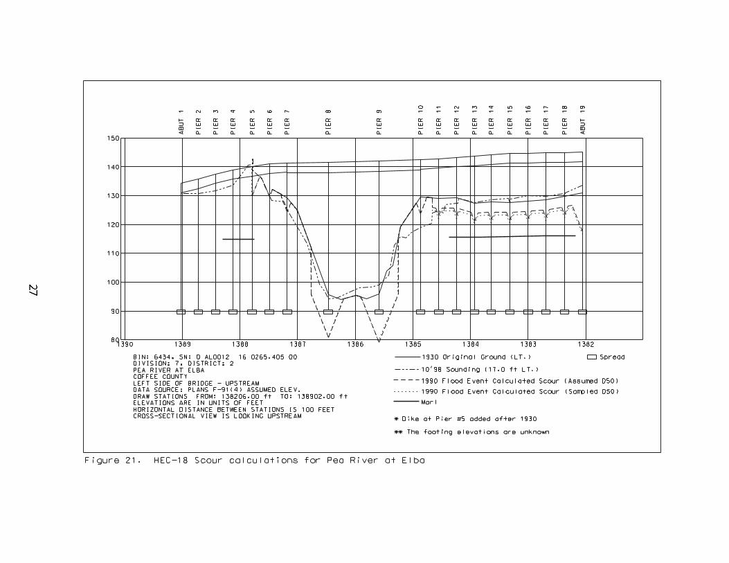
hard silt with clay (marl) below (Figure 5). A history of groundlines in the form of
soundings for the left and right side of the bridge were obtained that dated back to the
original groundline of 1930 (Figure 6 and 7). These provide a picture of what scour
occurred. Pictures taken after the 1998 flood indicated some contraction and local scour
shown in Figure 8.
Peak discharges were obtained from the USGS website (www.usgs.gov) since the
construction of the bridge (Figure 9 and Table 1). Peak discharges and daily discharges
did not exist from 1956 to 1971, and data before 1974 and during the 1980s was
unavailable. Only stage information was available for the 1990 event (largest event of
record) from the 1990 USGS Water Resources Data report. The stages were used to find
the discharges for the events using the current USGS rating curve developed for the site.

Bridge
Figure 1. USGS quadrangle map of the Pea River site at Elba, Alabama 07/01/1973

Figure 2. Aerial photo of Pea River at Elba
Bridge Site
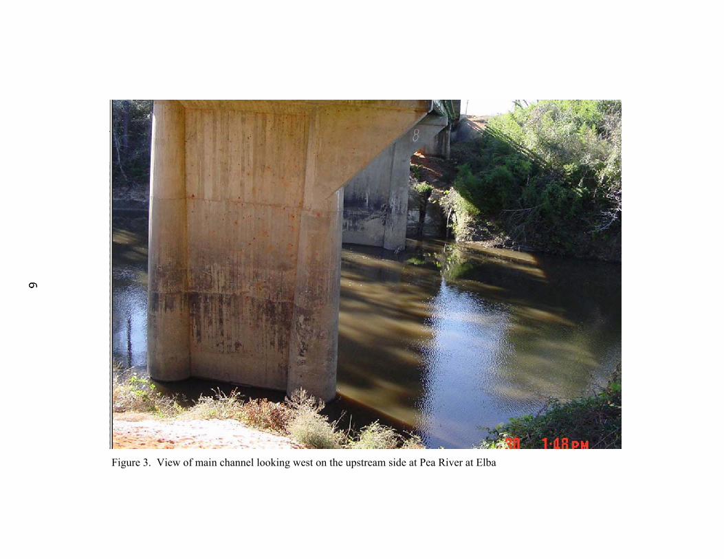
Figure 3. View of main channel looking west on the upstream side at Pea River at Elba

Figure 4. View of left overbank looking east on the downstream side at Pea River at Elba


View looking east upstream side of bridge
View looking west under bridge
Figure 8. Local scour under the bridge after the 1998 flood

Peak Discharges (cfs) - Pea River
0
10000
20000
30000
40000
50000
6000019
30
1933
1936
1939
1942
1945
1948
1951
1954
1957
1960
1963
1966
1969
1972
1975
1978
1981
1984
1987
1990
1992
1995
1999
Date
Dis
char
ge (c
fs)
Overbank flow
Figure 9. Peak discharges for Pea River at Elba

Table 1 Peak discharges for Pea River at Elba
Water Year Date
GageHeight(feet)
Stream-flow (cfs)
1929 Mar. 1929 43.50 90,0002,7
1930 1930 11,2002
1931 1931 7,6002
1932 1932 4,2002
1933 1933 13,8002
1934 1934 5,7002
1935 1935 5,6002
1936 Jan. 21, 1936 29.55 24,3001937 Apr. 06, 1937 30.00 25,0001938 Mar. 17, 1938 35.00 34,5001939 Feb. 28, 1939 20.80 12,9001940 Feb. 18, 1940 16.00 7,9001941 Mar. 07, 1941 10.23 3,5201942 Apr. 10, 1942 15.40 7,3501943 Jan. 19, 1943 26.80 20,4001944 Mar. 24, 1944 25.80 19,0001945 Apr. 29, 1945 12.80 5,2701946 May 21, 1946 22.30 14,6001947 Apr. 03, 1947 19.80 11,8001948 Mar. 07, 1948 21.20 13,3001949 Nov. 30, 1948 21.10 13,2001950 Sep. 01, 1950 15.00 7,0001951 Mar. 29, 1951 13.40 5,7201952 Mar. 27, 1952 17.80 9,6501953 Dec. 04, 1952 24.60 17,5001954 Jan. 01, 1954 11.79 4,5501955 Apr. 14, 1955 23.60 16,2001972 Mar. 03, 1972 19.70 11,700
WaterYear Date
Gage Height (feet)
Stream-flow (cfs)
1973 Mar. 12, 1973 27.00 20,7001974 Jan. 01, 1974 18.60 10,5001975 Feb. 19, 1975 37.26 38,2001976 May 15, 1976 19.90 11,9001977 Nov. 29, 1976 16.90 8,7501978 Jan. 26, 1978 28.60 22,9001979 Mar. 04, 1979 20.40 12,4001980 Mar. 13, 1980 19.15 11,1001981 Feb. 12, 1981 23.40 15,9001982 Feb. 04, 1982 16.55 8,4201983 May 20, 1983 21.35 13,5001984 Mar. 25, 1984 17.05 8,9001985 Feb. 06, 1985 19.00 10,9001986 Mar. 15, 1986 23.15 15,6001987 Feb. 28, 1987 14.55 6,6301988 Mar. 04, 1988 18.85 10,7001989 Jun. 17, 1989 18.30 10,2001990 Mar. 17, 1990 43.28 56,6001991 Jan. 31, 1991 19.30 11,2001992 Jan. 14, 1992 17.10 8,9501993 Nov. 26, 1992 18.33 10,2001994 Jul. 07, 1994 38.33 40,0001995 Feb. 12, 1995 21.40 13,6001996 Oct. 05, 1995 23.62 16,2001997 Feb. 15, 1997 16.91 8,7601998 Mar. 06, 1998 39.23 41,5001999 Mar. 14, 1999 20.51 12,6002000 Mar. 20, 2000 10.07 3,4302001 Mar. 04, 2001 22.70 15,100

Soil samples from core borings (Figure 10) were obtained from specific locations
at the bridge site (Figure 11). The samples were tested in an erosion function apparatus
(EFA) to determine the critical shear stress and the erosion function for each layer. More
details of the results of the tests will be discussed later and details of how the tests are
performed can be found in “Erosion Functions of Cohesive Soils,” by Crim (2003).

Figure 10. Drilling crew collecting samples at Pea River site at Elba

The second bridge site considered in this study is located on State Route 123 near
Newton, Alabama over the Choctawhatchee River (Figure 12 and 13). The bridge was
constructed in 1976. The bridge is 584 feet long with 10 spans and 9 piers. The drainage
area for the site is 686 square miles. The main channel (Figure 14) is approximately 150
feet wide with banks 20 to 25 feet high. The floodplain looking downstream is roughly
150 feet wide on the left overbank (Figure 15) and 225 feet wide on the right overbank.
Core borings at the site describe the soil on the right overbank to have sand on top with a
clay beneath and the left overbank to have a sandy clay on top with a clay beneath
(Figure 16). The main channel is a hard clay. A history of the groundlines in the form of
soundings for the left and right side of the bridge were obtained that dated back to 1976
(Figure 17 and 18).
Peak discharges were obtained since the construction of the bridge (Figure 19 and
Table 2). A history of daily discharges was also obtained from the USGS website dating
back to the construction date of the bridge.
Soil samples from core borings were obtained from specific locations at the
bridge site (Figure 20). The samples were tested in an erosion function apparatus (EFA).
After the collection of the preliminary data, one-dimensional hydraulic models
were constructed for both sites using HEC-RAS. Each model was analyzed with specific
discharges and stages taken incrementally from the rating curves. These runs provided
discharges per unit width, q, (q = Flowrate/TopWidth) and hydraulic depths, Yh, (Yh =
Area/TopWidth) for the main channel and for the overbanks for varying discharges and
stages. This data was used for interpolating q’s for the measured stages and discharges in
the main channel and in the overbanks.

Bridge
N
Figure 12. USGS quadrangle map of the Choctawhatchee River site near Newton, Alabama 07/01/1973

Figure 13. Aerial photo of Choctawhatchee River near Newton

Figure 14. View of main channel looking south on the downstream side at Choctawhatchee site near Newton

Figure 15. View of right overbank looking north on the upstream side at Choctawhatchee River site near Newton


Peak Discharges (cfs) - Choctawhatchee River
0
10000
20000
30000
40000
50000
60000
70000
80000
90000
100000
1976
1978
1980
1982
1984
1986
1988
1990
1992
1994
1996
1998
2000
Date
Disc
harg
e (c
fs)
Overbank Flow
Figure 19. Peak discharges for Choctawhatchee River near Newton

Table 2 Peak discharges Choctawhatchee River near Newton
Water Year Date
Gage Height(feet)
Stream- flow (cfs)
1976 Jan. 28, 1976 14.26 5,490
1977 Nov. 30, 1976 25.72 13,700
1978 Jan. 27, 1978 31.26 25,300
1979 Feb. 25, 1979 23.17 11,000
1980 Mar. 13, 1980 20.74 8,940
1981 Feb. 11, 1981 20.90 9,070
1982 Feb. 04, 1982 19.41 7,940
1983 Mar. 27, 1983 15.97 5,800
1984 May 04, 1984 17.23 6,490
1985 Feb. 07, 1985 24.21 12,000
1986 Mar. 15, 1986 15.46 5,730
1987 Mar. 30, 1987 11.58 3,690
1988 Mar. 05, 1988 17.03 6,620
1989 Jun. 16, 1989 11.00 3,410
1990 Mar. 18, 1990 40.30 87,500
1991 Feb. 01, 1991 22.10 10,100
1992 Mar. 07, 1992 15.58 5,790
1993 Nov. 27, 1992 21.46 9,520
1994 Jul. 07, 1994 37.78 60,800
1995 Feb. 12, 1995 21.78 9,790
1996 Mar. 19, 1996 17.86 7,110
1997 Jan. 09, 1997 18.38 7,430
1998 Mar. 09, 1998 34.58 39,200
1999 Oct. 01, 1998 21.51 9,560
2000 Feb. 14, 2000 8.70 2,350
2001 Mar. 05, 2001 24.02 11,800


III. PRESENT METHODOLOGY AND SCOUR CALCULATIONS
Pier, contraction, and abutment scour was previously calculated based on methods
from Hydraulic Engineering Circular 18 (HEC-18) for the two sites in a report by Curry
et al. (2002). The method assumes scour occurs very quickly and that maximum scour is
reached for each given discharge and stage. The calculated scour was plotted and can be
seen in Figures 21 and 22.
Each bridge site was modeled using HEC-RAS. The models are defined in HEC-
RAS as a series of cross-sections and associated parameters. Stream cross-sections were
obtained from the plan/profile sheet of the construction plans and from a sounding taken
by the USGS. Each cross-section was propagated approximately a bridge length
upstream and downstream of the site using the average slope of the channel estimated
from a USGS quadrangle map.
Several parameters were required to define the HEC-RAS model such as
Manning’s n-values and boundary conditions. Manning’s n-values were estimated for the
channel and overbank areas based on engineering judgment of the site. The n-values
were adjusted in some cases to calibrate the models to known depth averaged velocity
measurements. Discharges and starting downstream water surface elevations were two
boundary conditions needed in modeling the sites. The discharges and starting
downstream water surface elevations were taken from USGS records.


HEC-18 SCOUR CALCULATIONS
The hydraulic variables of the output of HEC-RAS were used to calculate scour
depths. HEC-RAS has built in routines for calculating scour based on methods described
in Hydraulic Engineering Circular No. 18 (HEC No. 18, FHWA, 1995). Contraction
scour and local scour (pier scour and abutment scour) were computed for each site.
As stated previously, all scour calculations were based on methods described in HEC-18.
The following section describes how scour was calculated with excerpts taken directly
from HEC-18 (FHWA, 1993, 1995, 2001) and the HEC-RAS Hydraulic Reference
Manual (Brunner, 2001b).
CONTRACTION SCOUR
As presented in HEC-18 and HEC-RAS, contraction scour occurs when the flow
area of a stream at flood stage is reduced, either by a natural contraction or a bridge. It
also occurs when overbank flow is forced back to the channel by roadway embankments
at the approaches to a bridge. The contraction of flow due to a bridge can be caused by
either a natural decrease in flow area of the stream channel or by abutments projecting
into the channel and/or piers blocking a portion of the flow area. Contraction can also be
caused by the approaches to a bridge cutting off floodplain flow. This flow from the
floodplain can cause clear-water scour on a setback portion of a bridge section or a relief
bridge because the floodplain flow does not normally transport significant concentrations
of bed material sediments. This clear-water picks up additional sediment from the bed
upon reaching the bridge opening. In addition, local scour at abutments may well be

greater due to the clear-water floodplain flow returning to the main channel at the end of
the abutment.
There are two conditions for contraction scour: clear-water and live-bed scour.
Clear-water scour occurs when the bed material sediment transport in the uncontracted
approach section is negligible or material transported through the contracted section is
mostly in suspension. Live-bed scour occurs when there is transport of bed material from
the upstream reach into the crossing.
Four conditions of contraction scour are commonly encountered:
Case 1. Involves overbank flow on a floodplain being forced back to the main channel by
the approaches to the bridge. Case 1 conditions include:
a. The river channel width becomes narrower either due to the bridge abutments
projecting into the channel or the bridge being located at a narrowing reach of
the river;
b. No contraction of the main channel, but the overbank flow area is completely
obstructed by an embankment; or
c. Abutments are set back from the stream channel.
Case 2. Flow is confined to the main channel (i.e., there is no overbank flow). The
normal river channel width becomes narrower due to the bridge itself or the bridge site is
located at a narrower reach of the river.
Case 3. A relief bridge in the overbank area with little or no bed material transport in the
overbank area (i.e., clear-water scour).

Case 4. A relief bridge over a secondary stream in the overbank area with bed material
transport (similar to case 1).
D50 values can be used to determine the velocity associated with the initiation of
motion, which in turn can be used as an indicator for clear-water or live-bed scour
conditions. If the mean velocity (V) in the upstream reach is equal to or less than the
critical velocity (Vc) of the median diameter (D50) of the bed material, then contraction
and local scour will be clear-water scour. Also, if the ratio of the shear velocity of the
flow to the fall velocity of the D50 of the bed material (V*/ω) is greater than 3,
contraction and local scour may be clear-water. If the mean velocity is greater than the
critical velocity of the median bed material size, live-bed scour will occur.
The following equation is used by HEC-RAS to calculate the critical velocity.
The derivation of the equation can be seen in HEC-18 (Second Edition, FHWA, 1993, p.
12).
3/150
6/1195.10 DyVc = (1)
Where:
Vc = Critical velocity above which bed material of size D50 and smaller will be transported, ft/s
1y = Average depth of flow in the main channel or overbank area at the approach section, ft
50D = Bed material particle size in a mixture of which 50% are smaller, ft
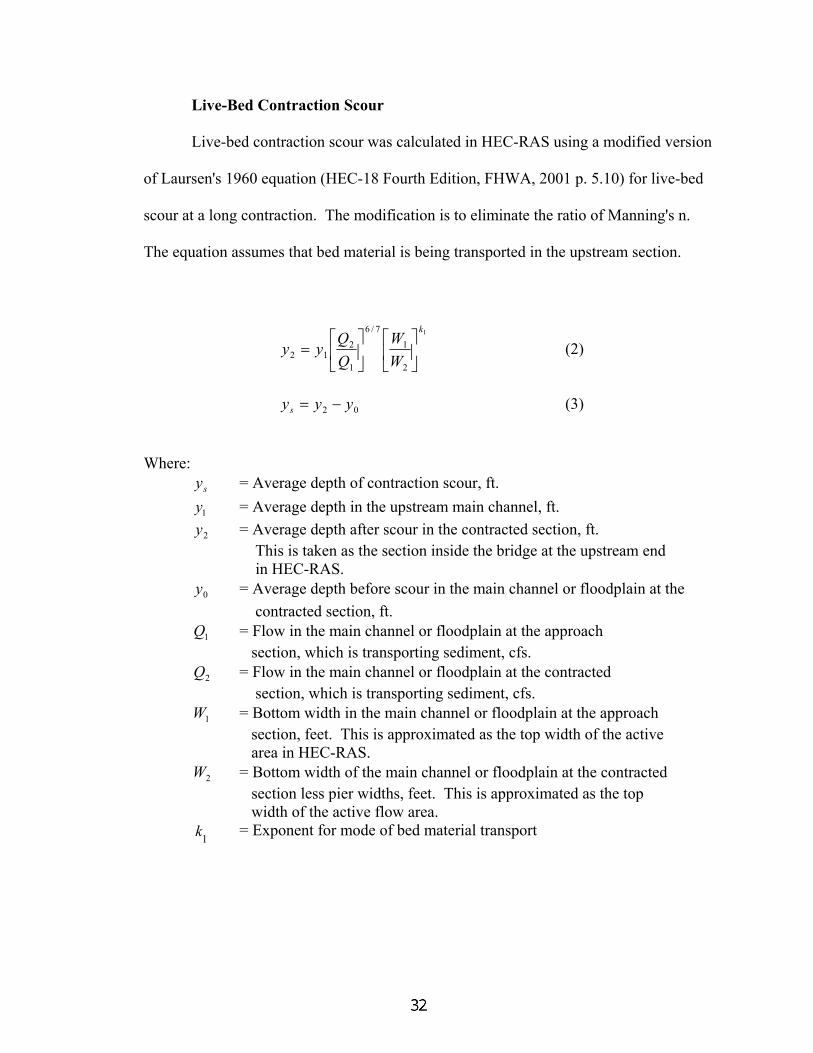
Live-Bed Contraction Scour
Live-bed contraction scour was calculated in HEC-RAS using a modified version
of Laursen's 1960 equation (HEC-18 Fourth Edition, FHWA, 2001 p. 5.10) for live-bed
scour at a long contraction. The modification is to eliminate the ratio of Manning's n.
The equation assumes that bed material is being transported in the upstream section.
1
2
1
7/6
1
212
k
WW
QQyy
= (2)
02 yyys −= (3)
Where: sy = Average depth of contraction scour, ft.
1y = Average depth in the upstream main channel, ft. = Average depth after scour in the contracted section, ft. 2y This is taken as the section inside the bridge at the upstream end in HEC-RAS. = Average depth before scour in the main channel or floodplain at the 0y contracted section, ft.
= Flow in the main channel or floodplain at the approach 1Q section, which is transporting sediment, cfs.
= Flow in the main channel or floodplain at the contracted 2Q section, which is transporting sediment, cfs.
= Bottom width in the main channel or floodplain at the approach 1W section, feet. This is approximated as the top width of the active area in HEC-RAS.
= Bottom width of the main channel or floodplain at the contracted 2W section less pier widths, feet. This is approximated as the top width of the active flow area.
= Exponent for mode of bed material transport k1

Table 3. Determining values for k1 V*/ω k1 Mode of Bed Material Transport <0.50 0.59 Mostly contact bed material discharge
0.50 to 2.0 0.64 Some suspended bed material discharge >2.0 0.69 Mostly suspended bed material discharge
V* = (τo/ρ)1/2 = (gy1 S1)1/2, shear velocity in the upstream section, ft/s ω = Fall velocity of bed material based on the D50, ft/s g = Acceleration of gravity, ft/s2 S1 = Slope of energy grade line of main channel, ft/ft
Clear-Water Contraction Scour
The following equation is used by HEC-RAS to calculate clear-water contraction
scour. The derivation of the equation can be seen in HEC-18 (Second Edition, FHWA,
1993, p. 12).
7/3
22
3/2
22
2
=
WCDQ
ym
(4)
02 yyys −= (5)
Where:
Dm = Diameter of the smallest non-transportable particle in the bed material (1.25D50) in the contracted section, ft.
D50 = Median diameter of the bed material, ft C = 120 for English units W2 = Bottom width of the bridge less pier widths, or overbank width (set back distance), ft

LOCAL SCOUR
Local Scour at Piers
Pier scour occurs due to acceleration of flow around the pier and the formation of
flow vortices (known as the horseshoe vortex). The horseshoe vortex removes material
from the base of the pier, creating a scour hole. The factors that affect the depth of local
scour at a pier are: velocity of the flow just upstream of the pier, depth of flow, width of
the pier, length of the pier if skewed to the flow, size and gradation of bed material, angle
of attack of approach flow, shape of pier, bed configuration, and the formation of ice
jams and debris.
HEC-RAS uses the Colorado State University (CSU) equation to calculate pier
scour under both live-bed and clear-water conditions. The equation is presented in HEC-
18 (Fourth Edition, FHWA, 2001, p. 6.4).
43.01
35.01
43210.2 FrayKKKK
ays
= (6)
Where: = Depth of scour in feet sy
= Correction factor for pier nose shape 1K = Correction factor for angle of attack of flow 2K = Correction factor for bed condition 3K = Correction factor for armoring of bed material 4K
= Pier width in feet a = Flow depth directly upstream of the pier in feet. 1y
= Froude Number directly upstream of the pier. 1FrFor round nose piers aligned with the flow, the maximum scour depth is limited as follows: 4 times the pier width (a) for .2≤sy 8.01 ≤Fr 0 times the pier width (a) for .3≤sy 8.01 >Fr

The correction factor for pier nose shape, , is given in Table 4: 1K
Table 4. Correction factor for pier nose shape Shape of Pier Nose 1K
Square nose 1.1 Round nose 1.0 Circular cylinder 1.0 Group of cylinders 1.0 Sharp nose (triangular) 0.9
The correction factor for the attack of the flow, , is calculated using the equation shown in HEC-18 (Fourth Edition, FHWA, 2001, p. 6.4):
2K
65.0
2 sincos
+= θθ
aLK (7)
Where: L = Length of the pier along the flow line, ft.
θ = Angle of attack of the flow, with respect to the pier.
If L/a is larger than 12, the program uses L/a = 12 as a maximum. If the angle of
attack is greater than 5 degrees, dominates and should be set to 1.0. 2K 1K
The correction factor for bed condition, , is shown in the table below: 3K
Table 5. Correction factor for bed condition
Bed Condition Dune Height H feet 3K
Clear-Water Scour N/A 1.1 Plane Bed and Antidune Flow N/A 1.1 Small Dunes 210 ≥> H 1.1 Medium Dunes 1030 ≥> H 1.1 to 1.2 Large Dunes H 30 1.3 The correction factor decreases scour depths for armoring of the scour hole for
bed materials that have a D
4K
50 equal to or larger than 0.20 feet. The correction factor
results from recent research by A. Molinas at CSU, which showed that when velocity (V1)

is less than the critical velocity (V ) of the D90c 90 size of the bed material, and there is a
gradation in sizes in the bed material, the D90 will limit the scour depth. The equations
are presented in HEC-18 (Third Edition, FHWA, 1993, pp. 37-38):
.0−
−−
cVV
90
1
645
195. Y
( )[ ] 5.024 1891 RVK −= (8)
where:
=
i
iR V
VV (9)
50
053.050.0 ci V
aD
V = (10)
V = Velocity ratio R
V = Average velocity in the main channel or overbank area at 1
the cross section just upstream of the bridge, ft/s V = Velocity when particles at a pier begin to move, ft/s i
V = Critical velocity for D90c 90 bed material size, ft/s V = Critical velocity for D50c 50 bed material size, ft/s a = Pier width, ft
3/16/10 cc DV = (11) where: Y = The depth of water just upstream of the pier, ft Dc = Critical particle size for critical velocity Vc, ft
Limiting K4 values and bed material size are given below:
Table 6. Limits for bed material size and K4 values
Factor Minimum Bed Material Size Minimum K4 Value VR>1.0
K4 2.050 ≥D ft 0.7 1.0

IV. CALCULATION OF SCOUR IN COHESIVE SOILS
SRICOS METHOD FOR PIER SCOUR
The Scour Rate in Cohesive Soils (SRICOS) method was introduced by Briaud et
al. (1999) for a constant approach velocity and a circular pier. The SRICOS method for
pier scour was later extended by Briaud et al. (2001b) for multiflood and multilayer
situations. In NCHRP report 24-15 by Briaud et al. (2003) the SRICOS method for pier
scour is further extended for use with complex piers.
The SRICOS method first consists of obtaining Shelby tube samples from the
bridge site and performing EFA tests on them to find the erosion function of the soil.
Then the maximum shear stress around a circular pier on a flat bottom is found with the
following equation,
2max
1 10.094 Vlog Re 10
τ ρ
= −
(12)
where ρ is the density of water (1000 kg/m3), V is the velocity of the water, and Re is the
Reynolds Number defined as VB/ν, where B is the pier diameter and ν is the kinematic
viscosity of water (10-6 m2/s at 20°C).
Once τmax is found the corresponding initial scour rate (żi) can be found from the
erosion function. The erosion function is the scour rate (ż) versus shear stress (τ) curve
that is found by doing soil tests using the EFA.
The maximum pier scour depth is the scour depth attained after a long time of
exposure to flood conditions. This depth may be better termed as the “ultimate” scour

depth (McLean et al., 2003 a, b). The equation for this maximum pier scour depth is
given by Briaud et al. (1999) as
( )0.635maxz 0.18mm Re= . (13)
The time variation of scour depth can now be calculated with the following
equation,
i ma
tz = 1 tz z
+x
(14)
where t is the length of time since the beginning of the flood starting with a flat bottom
around the pier. This function satisfies the condition z = 0 when t = 0, dz/dt → żi when
t → 0, and z → zmax when t → ∞.
E-SRICOS for Multiflood Conditions
In this method the time dependent hydrograph is broken into consecutive
segments of time intervals ∆t each with a constant approach velocity. For each time
interval, first an equivalent elapsed time t* is calculated as
1
i
1
max
zzt* = z1-
z
(15)
where z1 is the cumulative scour depth at the beginning of time interval ∆t, żi is the initial
scour rate for τmax obtained with a flat bottom corresponding to the approach velocity
during a time interval ∆t, and zmax is the maximum scour corresponding to the approach

( ) ( ) ( )0.126 1.706 0.20e hydro max it 73 t V z −=
velocity for time interval ∆t. The present equation 15 corresponds to equation 7 of
Briaud et al. (2001b), but with a different, simpler, form.
Once this t* is found for multifloods the cumulative scour depth at the end of the
time interval ∆t can be calculated as
2
i ma
t*+ tz z(t*+ t) = 1 t*+z z x
t∆
= ∆∆
+
(16)
where z2 is the cumulative scour depth at the end of time interval ∆t. The time variation
of cumulative scour is calculated in this manner using daily flows so the time interval ∆t
is one day.
S-SRICOS with Equivalent Time
The Simple SRICOS method was developed to do quick hand calculations to
predict the scour that would occur for a variable flow hydrograph of a long duration. To
do this an equivalent time (te) has to be found to substitute for t in equation 14 along with
the values of żi and zmax corresponding to maximum approach velocity of record. The
equation given by Briaud et al. (2001b) for calculating the equivalent time is
(17)
where thydro (yrs) is the number of years that the bridge has been built, Vmax is the
maximum velocity of record, and żi is the initial scour rate corresponding to τmax from
equation 12.

Square Piers
The equations above are all given for circular piers. To do the calculations for
square piers there are some shape factors from Briaud et al. (2003) that must be taken
into account. A shape factor must be multiplied into both τmax and zmax. The shape factor
that is multiplied into τmax (equation 12) is given as
L-4 B
shk 1.15 7e = + (18)
where L and B are the dimensions of the piers. In our case we only dealt with square
piers, so L = B. The shape factor that is given to be multiplied into zmax (equation 2) is
Ksh = 1.1. These shape factors enable us to use the equations for circular piers for square
piers by multiplying the equations by the appropriate shape factor.
Before access to the recent report by Briaud et al. (2003) we used another
approach to define an effective diameter for a square pier. This effective diameter was
calculated as
B = (19) a 2
where a is the width of the square pier.
SRICOS METHOD FOR CONTRACTION SCOUR
The SRICOS method for contraction scour is outlined by Briaud et al. (2003).
The calculations that were done for the SRICOS method in this report followed the same
procedures except for a few modifications.

In Briaud et at. (2003) the Manning n is used to get the bottom shear stress, while
we are using the Darcy-Weisbach friction factor to get bottom shear stress. The
maximum shear stress at the bottom is calculated using the equation,
2max hec
1 fV8
τ ρ= (20)
where ρ is the density of water (1000 kg/m3), Vhec is the velocity that comes from
HEC-RAS, and f = f (Recon) is the friction factor assuming a smooth boundary, where
Recon is the Reynolds number in the contraction defined as Recon = 4q/ν where q is the
flow per unit width and ν in the kinematic viscosity of water (10-6 m2/s at 20°C).
Once τmax is found the corresponding initial scour rate (żi) can be found from the
erosion function. The erosion function is the scour rate (ż) versus shear stress (τ) curve
that is found by doing soil tests using the EFA.
Now the ultimate value of the maximum scour depth in the contraction can be
found. In order to do this the critical Froude number and the Froude number
corresponding to the velocity in the contraction must be found. The critical Froude
number is calculated as
cc
h
8Frgfyτ
ρ= (21)
and the following equation is used to calculate the Froude number corresponding to the
velocity in the contraction,
hechec
h
VFrgy
= (22)

where τc is the critical shear stress of the soil, ρ is the density of water (1000 kg/m3), g is
acceleration due to gravity (9.81 m2/s), f is the friction factor, and yh is the water depth in
the contraction, and Vhec is the velocity that comes from HEC-RAS. Now the maximum
scour depth in the contraction can be calculated as
[ ]max hec c hz (Cont) = 1.90 1.49Fr Fr y− (23)
Briaud et al. (2003) also defined zunif (Cont), but we were only concerned with
zmax (Cont). This equation is equivalent to equation 7.9 in Briaud et al. (2003).
The time variation of scour depth can now be calculated with the following
equation,
i max
tz = 1 tz z (Cont)
+
(24)
where t is the length of time of the flood that scour is being calculated for.
E-SRICOS for Multiflood Conditions
The Extended SRICOS method for multiflood conditions had to be used in order
to calculate the cumulative contraction scour for the entire period of record as in the case
of pier scour, first an equivalent elapsed time, t* is calculated using the following
equation at each time step,
1
i
1
max
zzt* = z1-
z (Cont)
(25)
where z1 is the cumulative scour depth at the beginning of time interval ∆t, żi is the initial
scour rate for τmax corresponding to the approach velocity during the time interval ∆t, and
zmax is the ultimate scour depth for Recon corresponding to the approach velocity for time
interval ∆t.
Once this t* is found for multifloods the time variation of scour depth can then be
calculated as
2
i max
t*+ tz z(t*+ t) = 1 t*+ tz z (Cont)
∆= ∆
∆+
(26)
where z2 is the cumulative scour depth at the end of time interval ∆t.
DASICOS Method
The development of scour with time may also be calculated based on the rate of
scour given by the erosion function depending on the local value of the bed shear stress.
Because of its differential nature this approach may be called the DASICOS method
(Differential Analysis of Scour In Cohesive Soils) for the present purposes. Examples of
this approach have been presented in the recent studies of Güven et al. (2002a, b), Chen
(2002), and McLean et al. (2003a, b). Güven et al. (2002a, b) uses a one-dimensional
flow analysis while Chen (2002) uses a three-dimensional flow model. McLean et al.
(2003a, b) flow model is two-dimensional. In the present study an approach similar to
Güven et al. one-dimensional analysis is used.

In the DASICOS method the shear stress is calculated based on local conditions
with the following equation,
2
2
fq8yρτ = (27)
where ρ is the density of water (1000 kg/m3), q is the flow per unit width, y is the depth,
and f = f (Recon) is the friction factor assuming a smooth boundary. The Reynolds
number in the contraction is calculated as Recon = 4q/ν where q is the flow per unit width
and ν in the kinematic viscosity of water (10-6 m2/s at 20°C). The depth that is used in
the above equation is the scour depth added to the initial depth. The following equation
is used for this at each time step,
(28) hy(t) = y z(t)+
where y is the new depth, yh is the initial depth, and z is the scour for that time step.
The scour rate is defined as dz/dt and this is equal to R (τ) at any location. R is
the erosion function which gives the scour rate corresponding to the shear stress.
dz R( )dt
τ= (29)
The cumulative scour in the contraction is calculated by integrating equation 29 using
Euler’s method with the following equation,
2 1 1z z R( ) tτ= + ∆ (30)
where z2 is the cumulative scour depth at the end of time interval ∆t, z1 is the cumulative
scour depth at the beginning of time interval ∆t, τ1 is the shear stress corresponding to the
initial depth at time t1 and the average velocity during time interval ∆t, and R is the scour
rate corresponding to τ1 on the erosion function.

Ultimate Scour Depth
The ultimate scour depth can be found for any flood over an infinite time by first
calculating the ultimate water depth (yult) and subtracting the initial depth corresponding
to the flood (yh) from it,
(31) ult ult hz y= − y
where yult is calculated from the following equation,
2
ultc
fqy8ρ
τ= (32)
where ρ is the density of water (1000 kg/m3), q is the flow per unit width, τc is critical
shear stress from the erosion function, and f = f (Recon) is the friction factor assuming a
smooth boundary. The Reynolds number in the contraction is calculated as Recon = 4q/ν
where q is the flow per unit width and ν in the kinematic viscosity of water (10-6 m2/s at
20°C).
Programs
Programs were written in MATLAB to perform the above calculations. The code
for different methods can be found in Appendix A.

V. RATING FUNCTIONS FOR THE SITES
Stage-discharge rating curves were obtained from the USGS for both Pea River at
Elba (Figure 23) and Choctawhatchee River near Newton (Figure 24). Daily discharges
since the construction of the bridge were obtained from the USGS for the
Choctawhatchee River site only (Figure 25). We only used data through the 1990 flood
due to riprap being added immediately after it. A full set of hydrologic data did not exist
for Pea River at Elba. Hydraulic models were constructed for the sites. The cross-
sections were broken up into a left overbank, a right overbank, and a main channel
(Figure 26 and 27) due to the change in geometry across the sections. Incremental
discharges and stages were taken from the rating curves for determining flow
distributions for the overbanks and main channel. Top widths were taken for the
overbanks and main channel from the model to determine unit discharges, q
(Discharge/TopWidth). Hydraulic depths, yh (Area/TopWidth) were taken from the
model as well. Using discharge versus q data and discharge versus yh data, plots (found
in the Appendix B) were developed of stage versus q and stage versus yh. The
relationships were used to interpolate the q’s and the yh’s using the daily discharge
records. The entire record of the daily discharges for Choctawhatchee River near Newton
was filtered to discard the discharges less than 800 cfs in order to reduce the amount of
calculations. The critical shear stress is not exceeded until near 3000 cfs. The q and yh
data were used as input for the time dependent cohesive scour calculations.

Pea River at Elba
Stage vs Discharge
160
170
180
190
200
210
0 10000 20000 30000 40000 50000 60000 70000
Discharge (cfs)
Stag
e (f
t)
Figure 23 Stage vs discharge for Pea River at Elba
Choctawhatchee River Near NewtonStage vs Discharge
140145150155160165170175180
0 20000 40000 60000 80000 100000
Discharge (cfs)
Stag
e (f
t)
Figure 24. Stage vs discharge for Choctawhatchee River near Newton

Choctawhatchee River Near Newton, AlabamaDaily Discharge vs Time
0
10000
20000
30000
40000
50000
60000
70000
80000
0 1000 2000 3000 4000 5000 6000
Time (days)
Dis
char
ge (c
fs)
Figure 25. Daily discharges from 1975 to 1990

.04 .06 .06
138000 138200 138400 138600 138800150
160
170
180
190
200
210
Station (ft)
Ele
vatio
n (ft
)
Legend
WS March 9
0 ft/s
1 ft/s
2 ft/s
3 ft/s
4 ft/s
5 ft/s
6 ft/s
7 ft/s
8 ft/s
9 ft/s
10 ft/s
Main Channel
Left Overbank
Ground
Bank Sta
Right Overbank
Figure 26. Cross-section of Pea River at Elba
12500 13000 13500 14000 14500 15000 15500130
140
150
160
170
180
190
200
210
RS = 2.1 BR D
Station (ft)
Ele
vatio
n (ft
)
Legend
WS 50000
0 ft/s
1 ft/s
2 ft/s
3 ft/s
4 ft/s
5 ft/s
6 ft/s
7 ft/s
8 ft/s
9 ft/s
10 ft/s
Ground
Bank Sta
.15 .15 .15
Right Overbank
Main Channel
Left Overbank
Figure 27. Cross-section of Choctawhatchee River Near Newton

VI SOIL EXPLORATION AND EFA DATA FOR THE TWO SITES
The Alabama Department of Transportation (ALDOT) supplied the soil samples
used in this study. The samples were obtained in the field by pushing or driving an
ASTM standard Shelby tube with an outside diameter of 76.2 mm into the ground
(ASTM-D1587). ALDOT also supplied the boring logs with the samples. These logs
gave valuable information that was recorded during the actual sampling process. This
information included the depth at which the sample was taken, soil descriptions, and
blow counts (N). The blow counts were determined with standard penetration tests
(ASTM-D1586). Figure 28 shows the site sketch with core boring locations and Figure
29 shows the core borings for Pea River at Elba. Figure 30 shows the site sketch with
core boring locations and Figure 31 shows the core borings for Choctawhatchee River
near Newton.
The Samples were tested from the Pea River site at Elba and from the
Choctawhatchee River site near Newton. These samples are listed in TABLE 7 with
depths and soil descriptions taken from boring logs.


EFA TESTING
The EFA can be used for any type of soil which can be sampled with a standard
Shelby tube. It has been used for both coarse grained soils such as sands and for fine
grained soils such as clays. The EFA is used to find the erosion function of a soil. The
erosion function is the relation between the scour rate (ż) and the shear stress (τ) as
shown in Figure 32. The critical shear stress (τc) is the shear stress below which no scour
takes place. The initial erodibility (Si) indicates how fast the soil scours at the critical
shear stress and is the slope of a straight line tangent to the erosion function at the critical
shear stress.
Si = initial erodibility, ż = scour rate, τ = shear stress, τc = critical shear stress
Figure 32. Erosion function obtained from running an EFA test
Briaud et al. (1999, 2001a, 2001b) developed the EFA and the basic operating
procedures can be found in Briaud et al. (2001a). The EFA for this study (Figure 33) was
essentially the same as the EFA described by Briaud et al. (2001a), but there were some
differences that made the operating procedure a little different. A detailed description of

the EFA testing procedure can be found in Crim (2003). Figure 34 shows a sketch of the
important parts of the EFA.
FIGURE 33. Auburn University’s Erosion Function Apparatus (EFA)

FIGURE 34. Schematic showing the important parts of the EFA
To begin an EFA test the tank is filled with water and the prepared sample
installed in the EFA. The Shelby tube is held vertically over the piston and slowly
pushed down over the piston. Once the Shelby tube is in place over the piston it is
secured by tightening a clamp.

After the Shelby tube is securely in place the soil sample is brought to the top of
the tube by pushing the piston control on the EFA in the up position until the sample
comes out of the top of the Shelby tube. Once this is done the soil is trimmed evenly
with the top of the sampling tube.
The sample is then inserted into the rectangular conduit opening. The sample is
raised into the opening by using the crank wheel, aligned flush with the bottom of the
conduit, and the two screws on the platform tightened so that the Shelby tube cannot
move during testing (Figure 35).
FIGURE 35. Raising the Shelby tube into the conduit opening and placing it flush with the bottom using the crank wheel

The pump is turned on and the valve to regulate water velocity is opened allowing
flow through the conduit. The flow rate is measured by means of a propeller type flow
meter. The flow rate is combined with the cross sectional area of the pipe to compute the
average velocity of the flow.
After the velocity is set the soil is raised into the flow 1 mm in 0.5 mm
increments, which is controlled by the EFA computer. The computer records time,
average velocity, temperature, the soil sample advance that is pushed, and elapsed time.
The flow is maintained until 1 mm of soil is completely scoured away. The scour
is usually not uniform and the surface of the soil sample usually becomes uneven through
the duration of a test. Some of the exposed sample surface may have scoured more than
1 mm while some of it may have scoured less. When this happens the operator
subjectively decides when the scour is “on average” about 1 mm.
At the end of a test the pump is turned off and the water drains from the conduit.
The soil sample can then be lowered out of the conduit opening and prepared for the next
test. This is done by pushing some of the soil through the sampling tube and trimming it
even with the top of the tube. The sample is again raised into the opening and the test at
the next velocity is run. The test is repeated for between 5 and 8 velocities. By doing the
test at several velocities, the scour rate (mm/hr) vs. velocity (m/s) data is obtained. This
data is evaluated to give a scour rate (mm/hr) vs. shear stress (N/m2) relationship, which
is defined as the erosion function of the soil.

EFA TEST DATA REDUCTION AND PRESENTATION
The scour rate (ż) is the measure of how fast a particular soil erodes over time.
The scour rate for a particular soil with a set water velocity flowing over it can be
calculated from an EFA test. This scour rate is
ż = ∆h/∆t (33)
where ∆h is the length of soil eroded in a time ∆t. The length ∆h that is eroded during an
individual test at a specified velocity is 1 mm. The time ∆t is how long it takes for the 1
mm of soil sample to be eroded.
The shear stress applied by the water to the soil at the soil water interface is
generally considered to be the major parameter causing erosion (Briaud et al., 2001a).
The EFA does not directly give the shear stress applied to the soil. It does however give
velocity (V), which is related to the shear stress that the water imposes on the soil sample.
According to Briaud et al. (2001a) the best way to determine the shear stresses for
the EFA is by using the Moody chart which gives the relation between the pipe friction
factor f, the Reynolds Number Re, and the relative roughness ε/d where ε = roughness
height and d = pipe diameter. The Reynolds number is calculated as
VDReυ
= (34)
where V = average velocity in the pipe, D = 4Rh = hydraulic diameter of the pipe (Rh =
hydraulic radius), and υ = kinematic viscosity of water (10-6 m2/s at 20˚C).
After the Reynolds number is calculated the friction factor can be determined.
For the cohesive and fine-grained soils that were tested in this study the roughness was
considered to be smooth in the EFA. The equation that is used to calculate the friction
factor for smooth conditions is
( )1 2.0 log Re 0.8ff
= − . (35)
This equation was used for smooth conditions in Moody’s original paper (Moody, 1944).
An approximation of equation 35, called the Blasius equation (Henderson, 1966), that
was used for Re < 105 is
1/ 4
0.316Re
f = . (36)
This equation simplifies some of the calculations by making it possible to calculate f
directly if the Reynolds number is known. If Re > 105 then equation 35 is used to find
the friction factor. These are the equations for the smooth line on the Moody diagram
and make it possible to calculate the friction factor for a smooth surface without having
to go to the actual Moody diagram (Henderson, 1966).
The shear stress in the EFA is calculated as
2V
8fρτ = (37)
where τ = shear stress, f = friction factor from the Moody chart, ρ = mass density of water
(1000 kg/m3), and V = average velocity in the conduit.
Scour rate and shear stress are plotted to develop erosion functions for soils.
From these erosion functions, critical shear stress (τc), and initial erodibility (Si) are
determined. Best fit curves are visually determined for shear stresses greater than τc. The
erosion functions for the tested soils can be found in Appendix C.

SOIL CLASSIFICATION TESTING
Soils were tested to determine particle size and plasticity. Particle size analysis
was done using procedures in ASTM-D422 to determine D50. Plastic limits, liquid limits,
and plasticity indices (PI) of soils were determined using procedures in ASTM-D4318.
Results from these tests are contained in TABLE 7. Based on EFA tests, soil erosion
properties, τc, and Si , for the soils are also shown in TABLE 7.
TABLE 7. Soil properties for the tested soils.
Sample
Soil Description
Depth (ft)
D50 (mm)
PI (%)
τc
(N/m2)
Si (mm/hr)/(N/m2)
Choctawhatchee (1A) Gray Clay 10.0 - 12.0 0.027 24 2.5 0.96 Choctawhatchee (3B) Sand w/ Clay 5.0 - 7.0 0.15 6 0.65 9.5 Choctawhatchee (4B) Sand w/ Clay 6.8 - 8.0 0.32 NP* 0.46 10.4 Choctawhatchee (4C) Gray Silt w/ Clay 11.0 - 13.0 0.029 14 1.25 1.2
Pea (2A) Tan Clay 10.0 - 12.0 0.041 13 2.7 0.7 Pea (2B) Gray Silt 13.5 - 15.5 0.032 11 1.4 - Pea (3A) Gray Silt 10 - 11.5 0.034 NP* 1.5 3.7
* NP = Non-Plastic

VII. SCOUR EVALUATION AND RESULTS FOR PEA RIVER AT ELBA
Peak discharge and daily discharge data do not exist from 1956 to 1971; also,
data before 1974 and during the 1980s was unavailable. Only stage information was
available for the 1990 flood (largest event of record). The 1990 flood data came from the
USGS Water Resources Data reports. The stages were used to find the discharges for the
events using the current USGS rating curve developed for the site. The EFA results and
overbank’s unit discharges from the largest event of record indicated that no scour occurs
in the overbank because the critical shear stress is not exceeded. The soundings showed
that no scour occurred in the overbank on the left side of the bridge and minor scour
occurred on the right side of the bridge. The 1998 upstream sounding shows scour right
at the beginning of the left overbank near the main channel, but is probably due to the
exposed utility pipe that shows up in Figure 36. The downstream sounding shows no
scour. The 1998 flood which was lower than the 1990 flood showed 2-3 feet of local
scour between piers #10 and #12. A two-dimensional numerical model was constructed
of the site and shows high velocity zones in the shape of and in the area of the scoured
area (Figure 36). Blue indicates the higher velocities and red indicates the lower
velocities. Due to the lack of data, time dependent scour was not computed for this site.
Pier scour was computed for the main channel piers using the Simple SRICOS method
and can be seen in Figure 37. Field observations and soundings indicated no scour in the
main channel.

P11
P10 P12
P10
View 1 View 2
View 1 View 2
Bridge
Main Channel
Overbank
Figure 36. High velocity zones for the Pea River site at Elba and pictures after the 1998 flood event


VIII. SCOUR EVALUATION AND RESULTS FOR CHOCTAWHATCHEE RIVER NEAR NEWTON
Several methods for computing scour were performed for this site. Daily stream
flow data existed since construction. There was 6000 days of data from 1975 to 1990.
After the 1990 flood riprap was placed in the overbanks. Calculations were performed
for the filtered 2298 days of discharges from 1975 to 1990. The DASICOS method and
Extended SRICOS methods were used to calculate contraction scour in the left overbank
and in the main channel. Figures 38 and 39 show cumulative scour plots for the main
channel and Figures 40 and 41 show cumulative scour plots for the left overbank. The
plots show that DASICOS and E-SRICOS give similar results. The right overbank was
comprised of sand, which was previously calculated using HEC-18 methods.
The Simple SRICOS method and Extended SRICOS method for pier scour were
calculated for the two main channel piers and one overbank pier using an adaptation for
square piers and with the NCHRP Report 24-15 method Briaud et al. (2003). The results
of the Extended and Simple SRICOS pier scour calculations for the left overbank and the
main channel using both the adaptation for square piers and the NCHRP Report 24-15
method are shown in Figures 42 and 43. The adaptation for square piers, as described
earlier, gives similar results to the methods for complex piers described by Briaud et al.
(2003), which involve shape factors. This gives us more confidence that the shape
factors are reasonable. The added contraction and pier scour depths were plotted on the
bridge profile and are shown in Figure 44.

Figure 38. Choctawhatchee River near Newton contraction scour for the main channel.
0
0.1
0.2
0.3
0.4
0.5
0.6
0 500 1000 1500 2000 2500
Time (days)
Sco
ur (
m)
0
5
10
15
20
25
30
0 500 1000 1500 2000 2500
Time (days)
q (m
^2/s
)
DASICOS E-SRICOS

Figure 39. Choctawhatchee River near Newton contraction scour for the main channel
with ultimate scour depths plotted.
0
5
10
15
20
25
30
0 500 1000 1500 2000 2500
Time (days)
q (m
^2/s
)
02468
10121416
0 500 1000 1500 2000 2500
Time (days)
Sco
ur (
m)
DASICOS E-SRICOS zmax (Cont) zult

Figure 40. Choctawhatchee River near Newton contraction scour for the left overbank .
0
10
20
30
40
50
60
70
80
90
100
0 500 1000 1500 2000 2500
Time (days)
q (
ft^2
/s)
0
0.1
0.2
0.3
0.4
0.5
0.6
0.7
0.8
0 500 1000 1500 2000 2500
Time (days)
Sco
ur (
m)
DASICOS E-SRICOS

Figure 41. Choctawhatchee River near Newton contraction scour for the left overbank
with ultimate scour depths plotted.
0
10
20
30
40
50
60
70
80
90
100
0 500 1000 1500 2000 2500
Time (days)
q (
ft^2
/s)
0123456789
0 500 1000 1500 2000 2500
Time (days)
Sco
ur (m
)
DASICOS E-SRICOS zmax (Cont) zult

Figure 42. Choctawhatchee River near Newton pier scour for the main channel with
ultimate scour depths plotted.
0
5
10
15
20
25
30
0 500 1000 1500 2000 2500
Time (days)
q (m
^2/s
)
0
0.51
1.52
2.5
33.5
0 500 1000 1500 2000 2500
Time (days)
Sco
ur (
m)
E-SRICOS (effective diameter) E-SRICOS (shape factor) S-SRICOS (effective diameter) S-SRICOS (shape factor) zmax (effective diameter) zmax (shape factor)

Figure 43. Choctawhatchee River near Newton pier scour for the left overbank with
ultimate scour depths plotted.
0
10
20
30
40
50
60
70
80
90
100
0 500 1000 1500 2000 2500
Time (days)
q (
ft^2
/s)
0
0.5
1
1.5
2
2.5
3
0 500 1000 1500 2000 2500
Time (days)
Sco
ur (
m)
E-SRICOS (effective diameter) E-SRICOS (shape factor) S-SRICOS (effective diameter) S-SRICOS (shape factor) zmax (effective diameter) zmax (shape factor)


IX. CONCLUSIONS
The use of the EFA data and computational methods based on the scour rate for
cohesive soils improved the prediction results considerably. The calculated values of
scour for cohesive soils were in better agreement with the observed values compared with
the calculated values of scour using HEC-18 methods for noncohesive soils. This is
especially true for the left and right overbank of the Pea River site and the left overbank
and main channel of the Choctawhatchee River site. For the Pea River site the SRICOS
method shows very little pier scour and no contraction scour in the left overbank in
agreement with observations. Both the Simple SRICOS method and the HEC-18 method
show considerable scour around the main channel piers while observations show no
scour. The differences between the prediction and the observations in this case is most
likely due to incomplete information about the soil characteristics of the main channel. A
direct sample from the main channel could not be obtained, but a sample from a similar
depth to the main channel bed elevation was obtained from the overbank.
There is still some uncertainty about these results presented here due to the 3-D
nature of the actual flows and the variability of the soil properties at the sites. Additional
work with multidimensional numerical models and comparisons with more field data and
laboratory physical model experiments are needed.

REFERENCES
Briaud, J. L., Ting, F. C. K., Chen, H. C., Gudavalli, R., Perugu, S., and Wei, G. 1999. “SRICOS: Prediction of Scour Rate in Cohesive Soils at Bridge Piers,” Journal of Geotechnical and Geoenvironmental Engineering, Vol. 125, No. 4, April, pp. 237-246, American Society of Civil Engineers, Reston, Virginia, USA. Briaud, J. L., F. C. K. Ting, H. C. Chen, Y. Cao, S. W. Han, and K. W. Kwak, 2001a. “Erosion Function Apparatus for Scour Rate Predictions,” Journal of Geotechnical and Geoenvironmental Engineering, Vol. 127, No. 2, February, pp. 105-113, American Society of Civil Engineers, Reston, Virginia, USA. Briaud, J. L., H. C. Chen, K. W. Kwak, S. W. Han, and F. C. K. Ting, 2001b. “Multiflood and Multilayer Method for Scour Rate Prediction at Bridge Piers,” Journal of Geotechnical and Geoenvironmental Engineering, Vol. 127, No. 2, February, pp. 114-125, American Society of Civil Engineers, Reston, Virginia, USA. Briaud, J. L., H-C. Chen, Y. Li, P. Nurtjahyo, J. Wang, 2003. “Complex Pier Scour and Contraction Scour in Cohesive Soils,” NCHRP Report 24-15, Transportation Research Board National Research Council, National Cooperative Highway Research Program, January 2003. Brunner, G.W. 2001a. HEC-RAS, River Analysis System User’s Manual, US Army Corps of Engineers, Hydrologic Engineering Center, Report No. CPD 68, January 2001, Davis, C.A. Brunner, G.W., 2001b. HEC-RAS, River Analysis System Hydraulic Reference Manual, US Army Corps of Engineers, Hydrologic Engineering Center, Report No. CPD 69, January 2001, Davis, C.A. Chen, H-C., 2002. “Numerical Simulation of Scour Around complex Piers in Cohesive Soils,” ICSF-1 Vol. 1, November, pp. 14-33, Texas Transportation Institute, 2002, College Station, Texas, USA. Crim Jr., S., 2003. “Erosion Functions of Cohesive Soils,” Masters Thesis, August 2003, Auburn University, Alabama. Curry, J.E., O. Güven, J.G. Melville, and S. H. Crim, 2002. “Scour Evaluations of Selected Bridges in Alabama,” Highway Research Center 930-490, November 2002, Auburn University, Alabama. Federal Highway Administration, 1993. Evaluating Scour at Bridges, Federal Highway Administration, HEC No. 18, Publication No. FHWA-IP-90-017, 2nd Edition, April 1993, Washington D.C.

Federal Highway Administration, 1995. Evaluating Scour at Bridges, Federal Highway Administration, HEC No. 18, Publication No. FHWA-IP-90-017, 3rd Edition, November 1995, Washington D.C. Federal Highway Administration, 2001. Evaluating Scour at Bridges, Federal Highway Administration, HEC No. 18, Publication No. FHWA-NHI-01-001, 4th Edition, May 2001, Washington D.C. Güven, O., J.G. Melville, and J.E. Curry, 2001. Analysis of Clear-Water Scour At Bridge Contractions in Cohesive Soils, Highway Research Center IR-930-490, June 2001, Auburn University, Alabama. Güven, O., J.G. Melville, and J.E. Curry, 2002a. “Analysis of Clear-Water Scour at Bridge Contractions in Cohesive Soils”, TRB Paper No. 02-2127, Transportation Research Record, National Research Council, 2002, Washington, D.C. Güven, O., J.G. Melville, and J.E. Curry, 2002b. “Analysis of Clear-Water Scour at Bridge Contractions in Cohesive Soils”, ICSF-1 Vol. 1, pp. 14-33, Texas Transportation Institute, November 2002, College Station, Texas, USA. Henderson, F. M., 1966. “Open Channel Flow,” The Macmillan Company, New York. McLean, J.P., 2002a. “A Numerical Study of Flow and Scour in Open Channel Contractions,” Masters Thesis, May 2002, Auburn University, Alabama. McLean, J.P., O. Güven, J.G. Melville, and J.E. Curry, 2002b. “A Two Dimensional Numerical Model Study of Clear-Water Scour at Bridge Contraction with a Cohesive Bed,” Highway Research Center 930-490, April 2003, Auburn University, Alabama. Moody, L. F., 1944. “Friction Factors for Pipe Flow,” Transactions of the American Society of Mechanical Engineers, Vol. 66. Richardson, E.V., D.B. Simons, and P. Julien, 1990. Highways in the River Environment, FHWA-HI-90-016, Federal Highway Administration, U.S. Department of Transportation, February 1990, Washington, D.C.

Appendix A
MATLAB Computer Programs
All input and output of the programs are in metric.

MATLAB PROGRAM FOR DASICOS CONTRACTION SCOUR % DASICOS Method for contraction scour % Program reads q(t)and y(t) stage hydrograph from Excel file % Calculates transient scour (simple Euler method) format compact clear all % Enter excel finle name and sheet name H=xlsread('ChoctawLOB','Dataforrun'); % number of daily average flow measurements (q), dt = 1 day % yh is the downstream stage (depth) reading from exel file dt=1; D=2300; m=D/dt; for j=1:m t(j)=H(j,1); yh(j)=H(j,2); q(j)=H(j,3); end subplot(3,1,1) plot(t,q) hold grid ylabel('q (m^2/sec)') xlabel('Time (days)') subplot(3,1,2) plot(t,yh) hold grid xlabel('Time (days)') ylabel('Contraction Depth (m)') % Soil characteristics Si= 0.2496; Tc= 0.46; rho= 1000; g= 9.81; So= 0.04224; To= 0.75; D=0.00032; Ks=D/2; v = 10^-6;

% z(j)= cumulative scour depth. No scour as an initial condition z(1)=0; for j=1:m if q(j)>0 Y(j)=yh(j)+z(j); % Reynolds number Re= 4*q(j)/v; % Kr Kr= Ks/(4*Y(j)); % use Swamee-Jain Equation to find intial friction factor fr(1) = 0.25/((log10((Kr/3.7)+(5.74/Re^0.9)))^2); % use Henderson Equation to find friction factor for k=1:5 fr(k+1) = 0.25/((log10((Kr/3)+(2.5/(Re*fr(k)^.5))))^2); f(j)=fr(k+1); end % calculate the shear stress T(j)=(f(j)*rho*q(j).^2)/(8*Y(j)^2); % calculate the scour rate if T(j)>To R= Si*(To-Tc) + So*(T(j)-To); elseif T(j)>Tc R= Si*(T(j)-Tc); else R=0; end % Euler approximation of derivative z(j+1)=z(j)+R*dt; else z(j+1)=z(j); end t(j+1)=t(j)+dt; end

% write scour output to file that can be read with Excell dlmwrite('LOB.out',z',' ') [t;z]'; subplot(3,1,3) plot(t,z) hold plot(0,0) grid xlabel('Time (days)') ylabel('Scour Depth (m)') refresh

MATLAB Program for E-SRICOS Contraction Scour % E-SRICOS Method to calculate contraction scour format compact clear all % Enter Excel file name and sheet name H=xlsread('ChoctawLOB','Dataforrun'); % number of daily average flow measurements (q), dt = 1 day % yh is the downstream stage (depth) reading from Excel file dt=1; D=2300; m=D/dt; for J=1:m t(J)=H(J,1); yh(J)=H(J,2); q(J)=H(J,3); end subplot(3,1,1) plot(t,q) hold grid ylabel('q (m^2/sec)') xlabel('Time (days)') subplot(3,1,2) plot(t,yh) hold grid xlabel('Time (days)') ylabel('Contraction Depth (m)') % Soil characteristics Si= 0.2496; Tc= 0.46; rho= 1000; g= 9.81; So= 0.04224; To= 0.75; D=0.00032; Ks=D/2; v = 10^-6; g=9.81;

% z(j)= cumulative scour depth. No scour as an initial condition z(1)=0; for J=1:m if q(J)>0 % calculate velocity V(J)=q(J)./yh(J); % Reynolds number Re(J)= 4*q(J)/v; % Kr Kr(J)= Ks/(4*yh(J)); % use Swamee-Jain Equation to find intial friction factor fr(1) = 0.25/((log10((Kr(J)/3.7)+(5.74/Re(J)^0.9)))^2); % use Henderson Equation to find friction factor for k=1:5 fr(k+1) = 0.25/((log10((Kr(J)/3)+(2.5/(Re(J)*fr(k)^.5))))^2); f(J)=fr(k+1); end % calculate shear stress T(J)=(f(J)*rho*V(J).^2)/8; % calculate the critical Froude number Frc(J)=((8*Tc)/(rho*g*f(J)*yh(J)))^0.5; % calculate Froude number from velocity Fr(J)=V(J)/((g*yh(J))^0.5); else V(J)=0; Re(J)=0; T(J)=0; Frc(J)=0; Fr(J)=0; end

% calculate scour rate if T(J)>To R(J)= Si*(To-Tc) + So*(T(J)-To); else if T(J)>Tc R(J)=Si.*(T(J)-Tc); else R(J)=0; end end if R(J)>0 % calculate max scour depth for flow condition J zm(J)=yh(J)*1.9*((1.46*Fr(J))-Frc(J)); % calculate scour depth if z(J)>=zm(J) z(J+1)=z(J); else ts(J)=(z(J)/R(J))/(1-(z(J)/zm(J))); tss(J)=ts(J)+dt; z(J+1)=tss(J)/((1/R(J))+(tss(J)/zm(J))); end else z(J+1)=z(J); end t(J+1)=t(J)+dt; end % write scour output to file that can be read in Excell dlmwrite('LOBSRICOScontraction.out',z',' ') [t;z]' subplot(3,1,3) plot(t,z) grid on xlabel('Time (days)') ylabel('Scour Depth (m)') refresh

MATLAB Program for E-SRICOS Pier Scour % E-SRICOS Method to calculate pier scour format compact clear all % Enter Excel file name and sheet name H=xlsread('ChoctawLOB','Dataforrun'); % number of daily average flow measurements (q), dt = 1 day % yh is the downstream stage (depth) reading from Excel file dt=1; D=2300; m=D/dt; for J=1:m t(J)=H(J,1); yh(J)=H(J,2); q(J)=H(J,3); end subplot(3,1,1) plot(t,q) hold grid ylabel('q (m^2/sec)') xlabel('Time (days)') subplot(3,1,2) plot(t,yh) hold grid xlabel('Time (days)') ylabel('Contraction Depth (m)') % Pier characteristics for square in meters B= 1.1; L=B; % calculate shape factor for T (shear stress) ksh=1.15+(7*(exp(-4*(L/B)))); % shape factor for zm (max scour) Ksh=1.1;

% Soil characteristics Si= 0.2496; Tc= 0.46; rho= 1000; g= 9.81; So= 0.04224; To= 0.75; D=0.00032; Ks=D/2; v = 10^-6; % z(j)= cumulative scour depth. No scour as an initial condition z(1)=0; for J=1:m if q(J)>0 % calculate velocity V(J)=q(J)./yh(J); % Reynolds number Re(J)= B*V(J)/v; % calculate shear stress T(J)=ksh*0.094*rho.*V(J).^2*((1/log10(Re(J)))-(1/10)); else V(J)=0; Re(J)=0; T(J)=0; end % calculate scour rate if T(J)>To R(J)= Si*(To-Tc) + So*(T(J)-To); else if T(J)>Tc R(J)=Si.*(T(J)-Tc); else R(J)=0; end end

if R(J)>0 % calculate max scour depth for flow condition J zm(J)=(Ksh*0.18*(Re(J)^0.635))/1000; % calculate scour depth if z(J)>=zm(J) z(J+1)=z(J); else ts(J)=(z(J)/R(J))/(1-(z(J)/zm(J))); tss(J)=ts(J)+dt; z(J+1)=tss(J)/((1/R(J))+(tss(J)/zm(J))); end else z(J+1)=z(J); end t(J+1)=t(J)+dt; end % write scour output to file that can be read with Excel dlmwrite('LOBpierk.out',z',' ') [t;z]' subplot(3,1,3) plot(t,z) grid on xlabel('Time (days)') ylabel('Scour Depth (m)') refresh

Appendix B
Stream Flow Rating Functions
The cross-sections were broken up into a left overbank, a right overbank, and a main
channel due to the change in geometry across the sections. Incremental discharges (Q)
and stages were taken from the rating curve for determining flow distributions for the
overbanks and main channel. Top widths were taken for the overbanks and main channel
from the model to determine unit discharges, q (discharge/TopWidth). Hydraulic depths,
Yh (Area/top width) were taken from the model as well. Using discharge vs q and
discharge vs Yh, plots were developed of stage vs q, stage vs Yh, and stage vs V for the
overbanks and main channels. The anomalies in the curves come from changes in flow
distributions due to stages rising above the overbanks and coming in contact with the
underside of the bridges.

138000 138200 138400 138600 138800150
160
170
180
190
200
210
Station (ft)
Ele
vatio
n (ft
)
Legend
WS March 9
0 ft/s
1 ft/s
2 ft/s
3 ft/s
4 ft/s
5 ft/s
6 ft/s
7 ft/s
8 ft/s
9 ft/s
10 ft/s
Ground
Bank Sta
.04 .06 .06
Left Overbank Right Overbank
Main Channel
Cross-section and velocity distribution for one discharge and stage for Pea River at Elba

Pea River at Elba
Stage vs Discharge
160
170
180
190
200
210
0 10000 20000 30000 40000 50000 60000 70000
Discharge (cfs)
Stag
e (f
t)
Pea River at Elba
Main ChannelStage vs q
160
170
180190
200
210
0 50 100 150 200 250
q-Unit Discharge (sfs)
Stag
e (ft
)

Pea River at Elba
Main ChannelStage vs V
160
170
180
190
200
210
0 1 2 3 4 5 6 7
V-Velocity (fps)
Stag
e (ft
)
Pea River at Elba
Main Channel
160
170
180
190
200
210
0 10 20 30 40 5
Stag
e (ft
)
yh – Hydrualic Depth (ft)
0
Stage vs yh

Pea River at Elba
Left Overbank Stage vs q
160
170
180
190
200
210
0 10 20 30 40 50 6
q-Unit Discharge (sfs)
Stag
e (ft
)
0
Pea River at Elba
Left Overbank Stage vs V
160170
180
190
200210
0 1 2 3 4 5
V-Velocity (fps)
Stag
e (ft
)

Pea River at Elba
Left Overbank
160
170
180
190200
210
0 2 4
Stag
e (ft
)
yh
hh
160
170
180
190
200
210
0 5 10
Stag
e (ft
)
Stage vs YStage vs y
6 8 10 12 14 16
Yh-Hydraulic Depth (ft) – Hydrualic Depth (ft)
Pea River at ElbaRight Overbank
Stage vs q
15 20 25 30 35
q-Unit Discharge (sfs)

Pea River at ElbaRight Overbank
Stage vs V
160
170
180
190
200
210
0 0.5 1 1.5 2 2.5 3 3.5 4
V-Velocity (fps)
Stag
e (ft
)
Pea River at ElbaRight Overbank
160
170
180
190
200
210
0 2 4 6 8 10 12 1
Stag
e (ft
)
yh – Hydrualic Depth (ft) 4
Stage vs yh

12500 13000 13500 14000 14500 15000 15500130
140
150
160
170
180
190
200
210
RS = 2.1 BR D
Station (ft)
Ele
vatio
n (ft
)Legend
WS 50000
0 ft/s
1 ft/s
2 ft/s
3 ft/s
4 ft/s
5 ft/s
6 ft/s
7 ft/s
8 ft/s
9 ft/s
10 ft/s
Ground
Bank Sta
.15 .15 .15
Right Overbank
Main Channel
Left Overbank
Cross-section and velocity distribution for one discharge and stage for Choctawhatchee River near Newton

Choctawhatchee River Near Newton
Stage vs Discharge
140145150155160165170175180
0 20000 40000 60000 80000 100000
Discharge (cfs)
Stag
e (f
t)
Choctawhatchee River Near Newton
Main ChannelStage vs q
140
150
160
170
180
0 50 100 150 200 250 300 350
q-Unit Discharge (sfs)
Stag
e (ft
)

Choctawhatchee River Near Newton
Main ChannelStage vs V
140
150
160
170
180
0 2 4 6 8 10 1
V-Velocity (fps)
Stag
e (ft
)
2
Choctawhatchee River Near Newton
Main Channel
140
150
160
170
180
0 5 10 15 20 25 30 35
Stag
e (ft
)
yh – Hydrualic Depth (ft)
Stage vs yh

Choctawhatchee River Near Newton
Left Overbank Stage vs q
140
150
160
170
180
0 20 40 60 80 100 12
q-Unit Discharge (sfs)
Stag
e (ft
)
0
Choctawhatchee River Near Newton
Left Overbank Stage vs V
140
150
160
170
180
0 1 2 3 4 5 6 7 8
V-Velocity (fps)
Stag
e (ft
)

Choctawhatchee River Near Newton
Left Overbank
140
150
160
170
180
0 2 4 6 8 10 12 14 16
Stag
e (ft
)
yh – Hydrualic Depth (ft)
Stage vs yh

Appendix C
Erosion Functions

τ (N/m2)
0 5 10 15 20
Scou
r Rat
e (m
m/h
r)
0
5
10
15
τc = 2.7 N/m2
Si = 0.7 mm/hr/N/m2
Pea River at Elba Sample 2A
τc (N/m2)
0.0 0.5 1.0 1.5 2.0
Scou
r Rat
e (m
m/h
r)
0.0
0.5
1.0
τc = 1.4 N/m2
Si = could not be determined due to soil breaking off in large pieces
Pea River at Elba Sample 2B

τ (N/m2)
0 1 2 3 4 5 6
Scou
r Rat
e (m
m/h
r)
0
2
4
6
8
10
12
τc = 1.5 N/m2
Si = 3.7 mm/hr/N/m2
Pea River at Elba Sample 3A
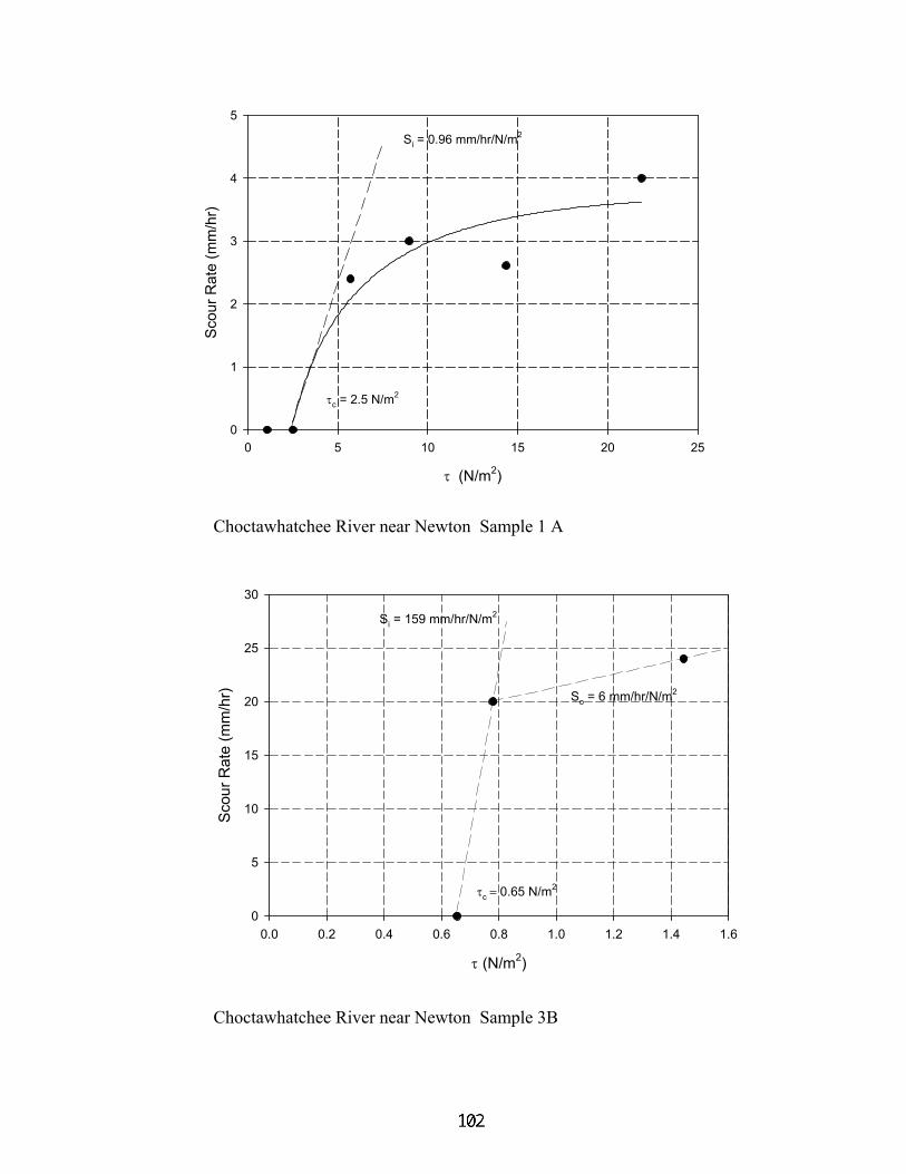
Appendix B
τ (N/m2)
0 5 10 15 20 25
Sco
ur R
ate
(mm
/hr)
0
1
2
3
4
5
Si = 0.96 mm/hr/N/m2
τc = 2.5 N/m2
Choctawhatchee River near Newton Sample 1 A
τ (N/m2)
0.0 0.2 0.4 0.6 0.8 1.0 1.2 1.4 1.6
Sco
ur R
ate
(mm
/hr)
0
5
10
15
20
25
30
τc = 0.65 N/m2
Si = 159 mm/hr/N/m2
So = 6 mm/hr/N/m2
Choctawhatchee River near Newton Sample 3B

τ (N/m2)
0.0 0.2 0.4 0.6 0.8 1.0 1.2 1.4
Sco
ur R
ate
(mm
/hr)
0
1
2
3
4
5
τc = 0.46 N/m2
Si = 10.4 mm/hr/N/m2
So = 1.76 mm/hr/N/m2
Choctawhatchee River Near Newton Sample 4B
τ (N/m2)
0 5 10 15 20
Scou
r Rat
e (m
m/h
r)
0
5
10
15
20
τc = 1.25 N/m2
Si = 1.2 mm/hr/N/m2
Choctawhatchee River Near Newton Sample 4C