Embed Size (px)
Citation preview

Oscilloscope FundamentalsOscilloscope Fundamentals
For Electrical Engineering and Physics Undergraduat e Students

AgendaAgenda What is an oscilloscope?
Probing basics (low -frequency model)
Making voltage and timing measurements
Properly scaling waveforms on-screen
Understanding oscilloscope triggering
Oscilloscope theory of operation and performance specifications
Probing revisited (dynamic/AC model and affects of loading)
Using the DSOXEDK Lab Guide and Tutorial
Additional technical resources
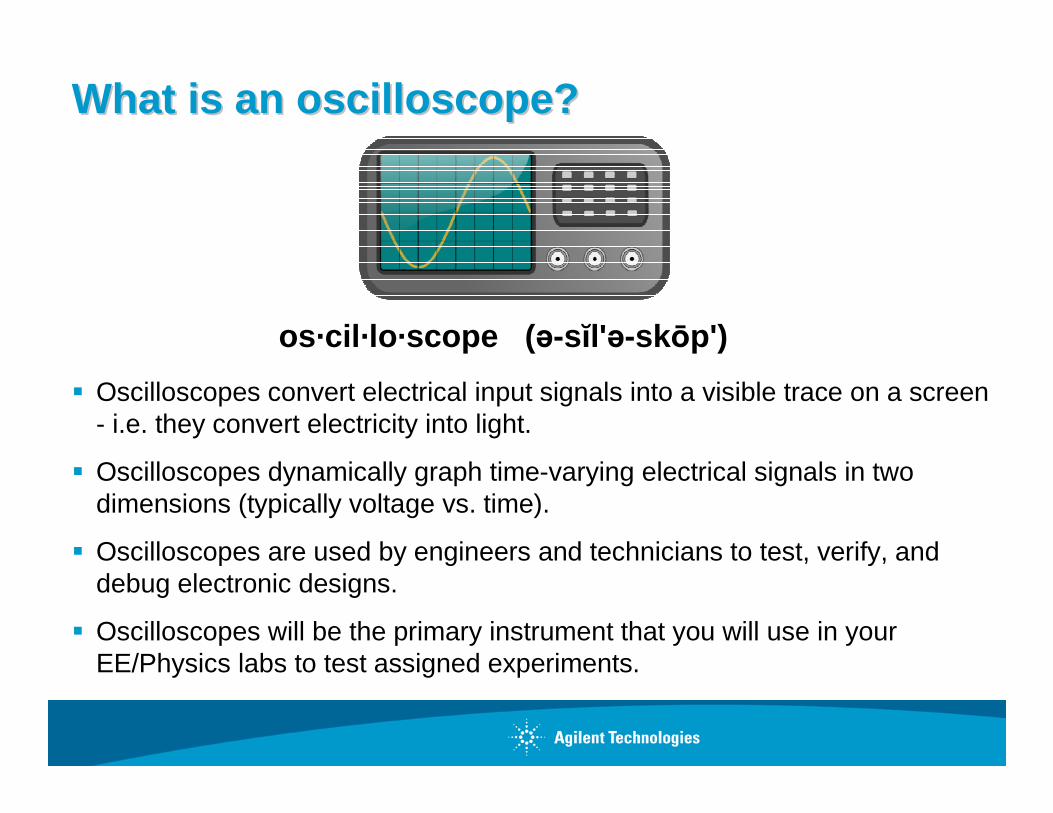
What is an oscilloscope?What is an oscilloscope?
Oscilloscopes convert electrical input signals into a visible trace on a screen - i.e. they convert electricity into light.
Oscilloscopes dynamically graph time-varying electrical signals in two dimensions (typically voltage vs. time).
Oscilloscopes are used by engineers and technicians to test, verify, and debug electronic designs.
Oscilloscopes will be the primary instrument that you will use in your EE/Physics labs to test assigned experiments.
os·cil·lo·scope ( ə-sĭl'ə-skōp')
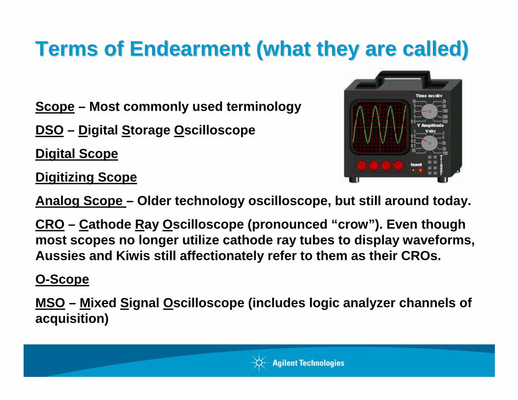
Terms of Endearment (what they are called)Terms of Endearment (what they are called)
Scope – Most commonly used terminology
DSO – Digital S torage O scilloscope
Digital Scope
Digitizing Scope
Analog Scope – Older technology oscilloscope, but still around to day.
CRO – Cathode R ay Oscilloscope (pronounced “crow”). Even though most scopes no longer utilize cathode ray tubes to display waveforms, Aussies and Kiwis still affectionately refer to the m as their CROs.
O-Scope
MSO – Mixed S ignal O scilloscope (includes logic analyzer channels of acquisition)

Probing BasicsProbing Basics
Probes are used to transfer the signal from the device-under-test to the oscilloscope’s BNC inputs.
There are many different kinds of probes used for different and special purposes (high frequency applications, high voltage applications, current, e tc.).
The most common type of probe used is called a “Passive 10:1 Voltage Divider Probe”.
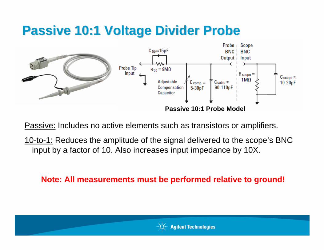
Passive 10:1 Voltage Divider ProbePassive 10:1 Voltage Divider Probe
Passive: Includes no active elements such as transistors or amplifiers.
10-to-1: Reduces the amplitude of the signal delivered to the scope’s BNC input by a factor of 10. Also increases input impedance by 10X.
Note: All measurements must be performed relative t o ground!
Passive 10:1 Probe Model
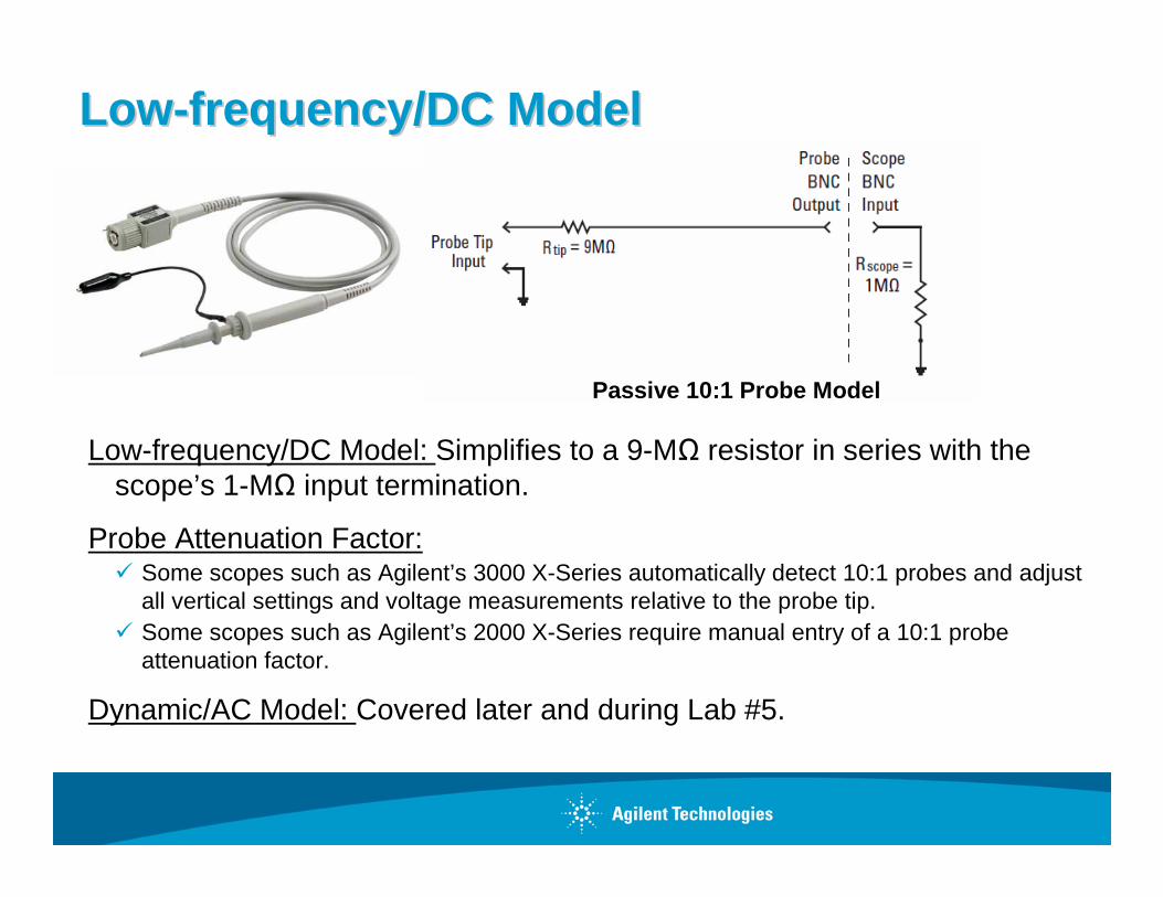
LowLow --frequency/DC Modelfrequency/DC Model
Low-frequency/DC Model: Simplifies to a 9-MΩ resistor in series with the scope’s 1-MΩ input termination.
Probe Attenuation Factor: Some scopes such as Agilent’s 3000 X-Series automatically detect 10:1 probes and adjust
all vertical settings and voltage measurements relative to the probe tip. Some scopes such as Agilent’s 2000 X-Series require manual entry of a 10:1 probe
attenuation factor.
Dynamic/AC Model: Covered later and during Lab #5.
Passive 10:1 Probe Model

Understanding the ScopeUnderstanding the Scope ’’s Displays Display
Waveform display area shown with grid lines (or divisions).
Vertical spacing of grid lines relative to Volts/division setting.
Horizontal spacing of grid lines relative to sec/division setting.
Vol
ts
Time
Vertical = 1 V/div Horizontal = 1 µs/div1 Div
1 D
iv

Making Measurements Making Measurements –– by visual estimationby visual estimation
Period (T) = 4 divisions x 1 µs/div = 4 µs, Freq = 1/T = 250 kHz. V p-p = 6 divisions x 1 V/div = 6 V p-p V max = +4 divisions x 1 V/div = +4 V, V min = ?
V p
-p
Period
Vertical = 1 V/div Horizontal = 1 µs/div
V m
ax
Ground level (0.0 V) indicator
The most common measurement technique
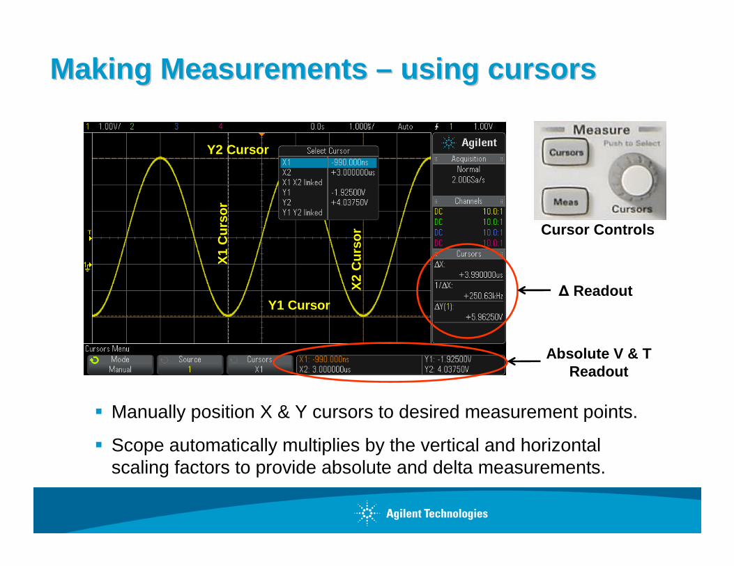
Making Measurements Making Measurements –– using cursorsusing cursors
Manually position X & Y cursors to desired measurement points.
Scope automatically multiplies by the vertical and horizontal scaling factors to provide absolute and delta measurements.
X1
Cur
sor
X2
Cur
sor
Y1 Cursor
Y2 Cursor
∆ Readout
Absolute V & T Readout
Cursor Controls

Making Measurements Making Measurements –– using the scopeusing the scope ’’s s automatic parametric measurementsautomatic parametric measurements
Select up to 4 automatic parametric measurements with a continuously updated readout.
Readout
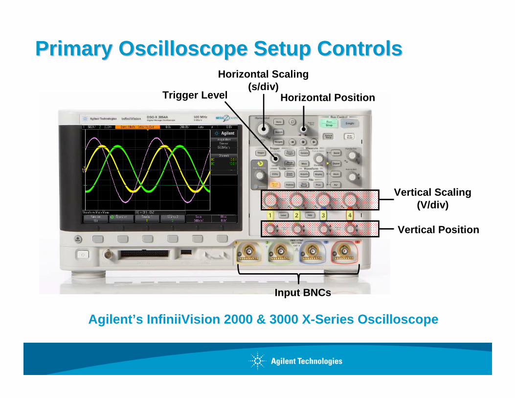
Primary Oscilloscope Setup ControlsPrimary Oscilloscope Setup ControlsHorizontal Scaling
(s/div)Horizontal Position
Vertical Position
Vertical Scaling (V/div)
Input BNCs
Trigger Level
Agilent’s InfiniiVision 2000 & 3000 X-Series Oscillos cope
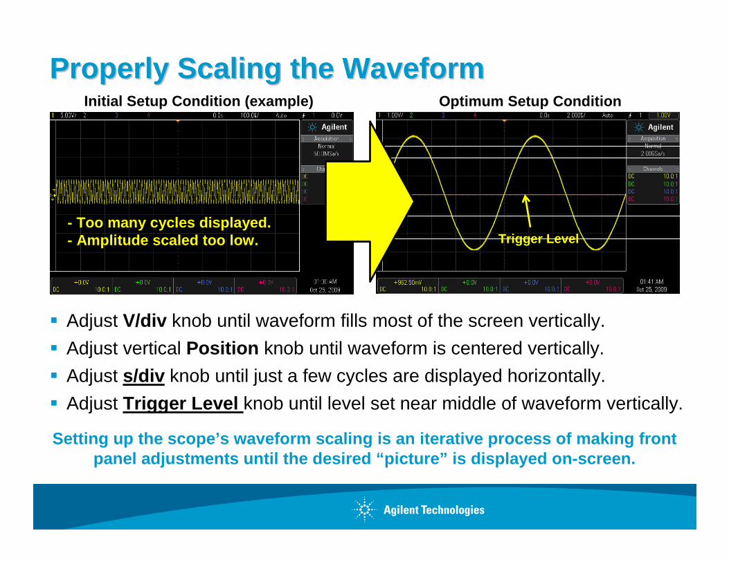
Properly Scaling the WaveformProperly Scaling the Waveform
Adjust V/div knob until waveform fills most of the screen vertically.
Adjust vertical Position knob until waveform is centered vertically.
Adjust s/div knob until just a few cycles are displayed horizontally.
Adjust Trigger Level knob until level set near middle of waveform vertically.
- Too many cycles displayed.- Amplitude scaled too low.
Initial Setup Condition (example) Optimum Setup Condition
Trigger Level
Setting up the scope’s waveform scaling is an iterat ive process of making front panel adjustments until the desired “picture” is dis played on-screen.

Understanding Oscilloscope TriggeringUnderstanding Oscilloscope Triggering
Think of oscilloscope “triggering” as “synchronized picture taking”.
One waveform “picture” consists of many consecutive digitized samples.
“Picture Taking” must be synchronized to a unique point on the waveform that repeats.
Most common oscilloscope triggering is based on synchronizing acquisitions (picture taking) on a rising or falling edge of a signal at a specific voltage level.
Triggering is often the least understood function o f a scope, but is one of the most important capabilities that you sho uld understand.
A photo finish horse race is analogous to oscilloscope
triggering

Triggering ExamplesTriggering Examples
Default trigger location (time zero) on DSOs = cent er-screen (horizontally)
Only trigger location on older analog scopes = left side of screen
Trigger Point
Trigger Point
Untriggered(unsynchronized picture taking)
Trigger = Rising edge @ 0.0 V
Trigger = Falling edge @ +2.0 V
Trigger level set above waveform
Positive TimeNegative Time
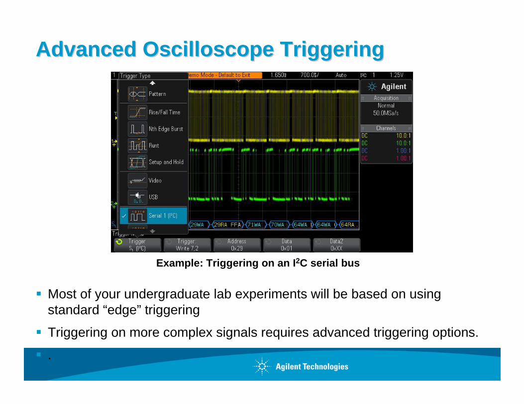
Advanced Oscilloscope TriggeringAdvanced Oscilloscope Triggering
Most of your undergraduate lab experiments will be based on using standard “edge” triggering
Triggering on more complex signals requires advanced triggering options.
.
Example: Triggering on an I 2C serial bus

Oscilloscope Theory of OperationOscilloscope Theory of Operation
DSO Block Diagram
Yellow = Channel-specific blocksBlue = System blocks (supports all channels)
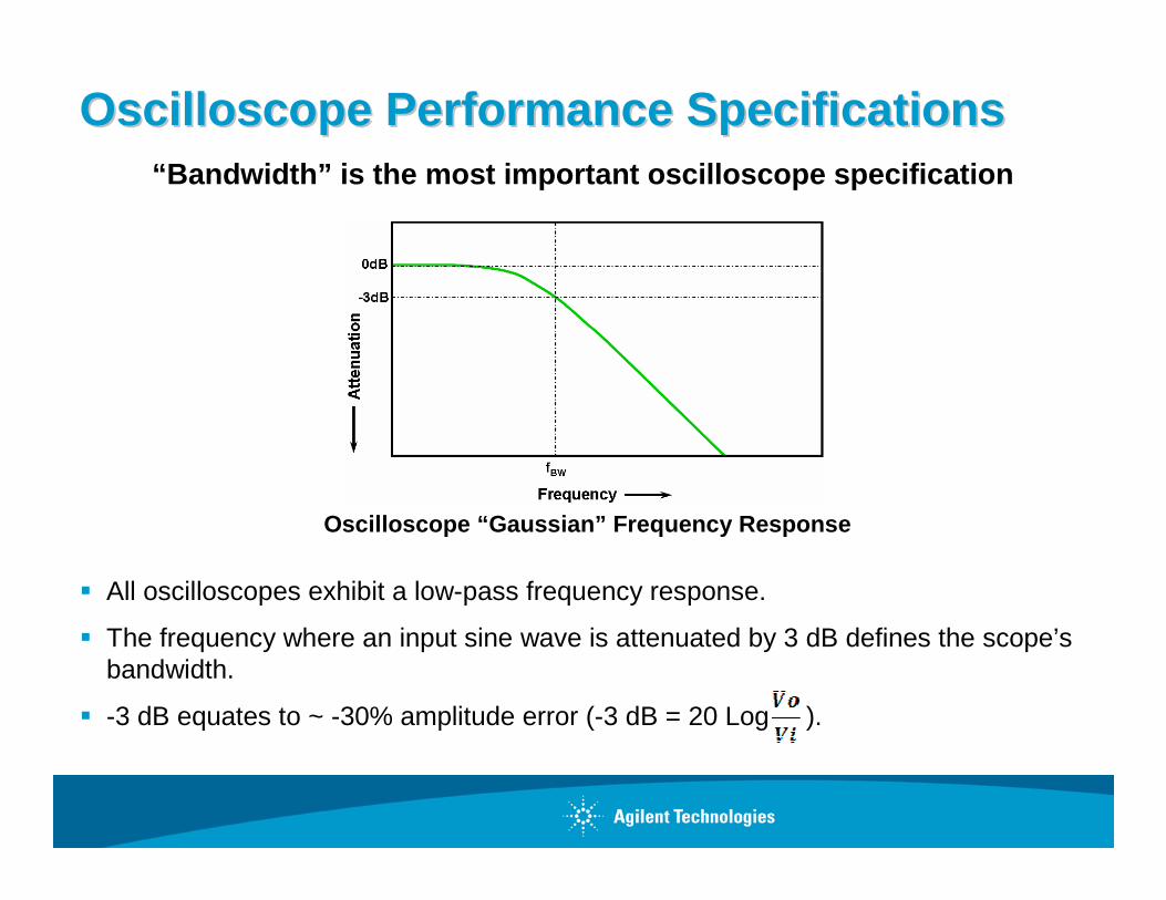
Oscilloscope Performance SpecificationsOscilloscope Performance Specifications
All oscilloscopes exhibit a low-pass frequency response.
The frequency where an input sine wave is attenuated by 3 dB defines the scope’s bandwidth.
-3 dB equates to ~ -30% amplitude error (-3 dB = 20 Log ).
Oscilloscope “Gaussian” Frequency Response
“Bandwidth” is the most important oscilloscope speci fication
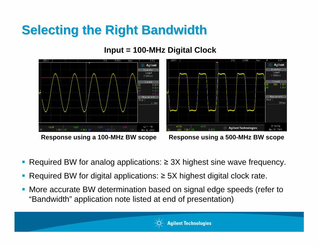
Selecting the Right BandwidthSelecting the Right Bandwidth
Required BW for analog applications: ≥ 3X highest sine wave frequency.
Required BW for digital applications: ≥ 5X highest digital clock rate.
More accurate BW determination based on signal edge speeds (refer to “Bandwidth” application note listed at end of presentation)
Response using a 100-MHz BW scope
Input = 100-MHz Digital Clock
Response using a 500-MHz BW scope
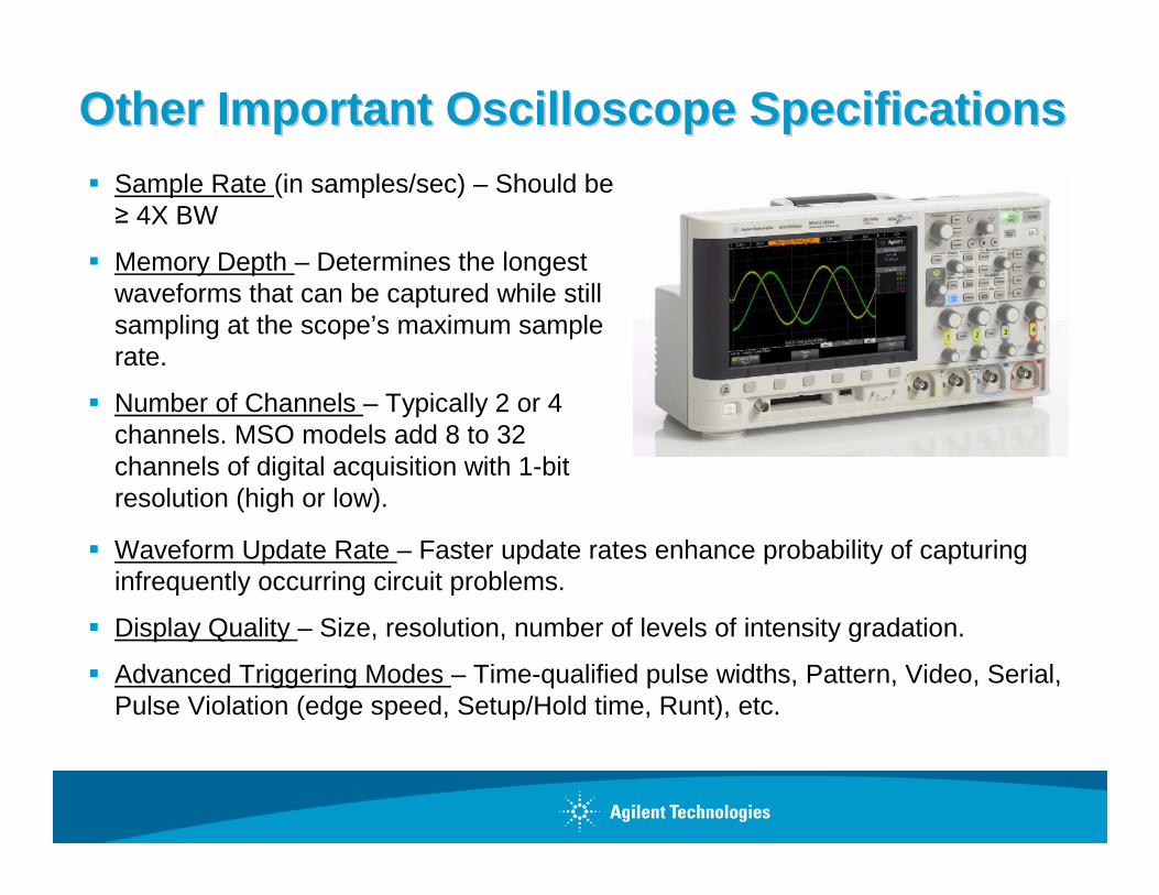
Other Important Oscilloscope SpecificationsOther Important Oscilloscope Specifications Sample Rate (in samples/sec) – Should be ≥ 4X BW
Memory Depth – Determines the longest waveforms that can be captured while still sampling at the scope’s maximum sample rate.
Number of Channels – Typically 2 or 4 channels. MSO models add 8 to 32 channels of digital acquisition with 1-bit resolution (high or low).
Waveform Update Rate – Faster update rates enhance probability of capturing infrequently occurring circuit problems.
Display Quality – Size, resolution, number of levels of intensity gradation.
Advanced Triggering Modes – Time-qualified pulse widths, Pattern, Video, Serial, Pulse Violation (edge speed, Setup/Hold time, Runt), etc.

Probing Revisited Probing Revisited -- Dynamic/AC Probe ModelDynamic/AC Probe Model
Cscope and Ccable are inherent/parasitic capacitances (not intentionally designed-in)
Ctip and Ccomp are intentionally designed-in to compensate for Cscope and Ccable .
With properly adjusted probe compensation, the dynamic/AC attenuation due to frequency-dependant capacitive reactances should match the designed-in resistive voltage-divider attenuation (10:1).
Passive 10:1 Probe Model
Where Cparallel is the parallel combination of C comp + Ccable + Cscope
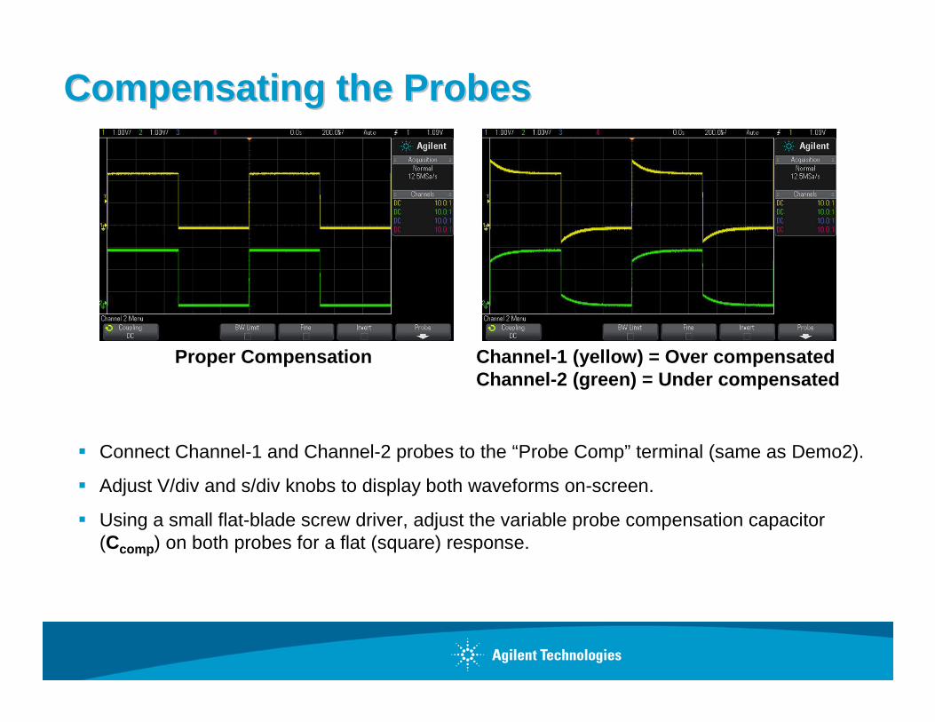
Compensating the ProbesCompensating the Probes
Connect Channel-1 and Channel-2 probes to the “Probe Comp” terminal (same as Demo2).
Adjust V/div and s/div knobs to display both waveforms on-screen.
Using a small flat-blade screw driver, adjust the variable probe compensation capacitor(Ccomp ) on both probes for a flat (square) response.
Proper Compensation Channel-1 (yellow) = Over compensatedChannel-2 (green) = Under compensated

Probe LoadingProbe Loading
The probe and scope input model can be simplified down to a single resistor and capacitor.
Any instrument (not just scopes) connected to a circuit becomes a part of the circuit under test and will affect measured results… especially at higher frequencies.
“Loading” implies the negative affects that the scope/probe may have on the circuit’s performance.
CLoad
Probe + Scope Loading Model
RLoad

AssignmentAssignment
1. Assuming Cscope = 15pF, Ccable = 100pF and Ctip = 15pF, compute Ccomp if properly adjusted. Ccomp = ______
2. Using the computed value of Ccomp , compute CLoad . CLoad = ______
3. Using the computed value of CLoad , compute the capacitive reactance of CLoadat 500 MHz. XC-Load = ______
C Load = ?
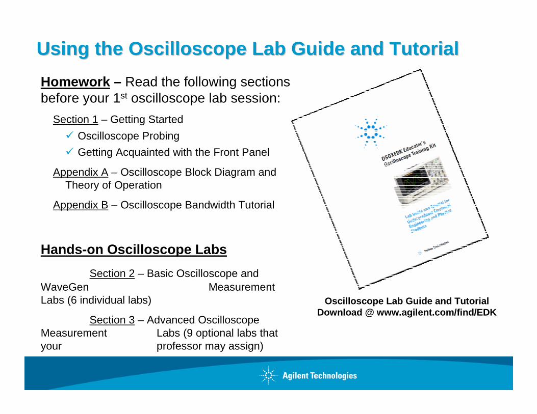
Using the Oscilloscope Lab Guide and TutorialUsing the Oscilloscope Lab Guide and Tutorial
Homework – Read the following sections before your 1st oscilloscope lab session:
Section 1 – Getting Started
Oscilloscope Probing
Getting Acquainted with the Front Panel
Appendix A – Oscilloscope Block Diagram and Theory of Operation
Appendix B – Oscilloscope Bandwidth Tutorial
Hands-on Oscilloscope Labs
Section 2 – Basic Oscilloscope and WaveGen Measurement Labs (6 individual labs)
Section 3 – Advanced Oscilloscope Measurement Labs (9 optional labs that your professor may assign)
Oscilloscope Lab Guide and TutorialDownload @ www.agilent.com/find/EDK

Hints on how to follow lab guide instructionsHints on how to follow lab guide instructions
Bold words in brackets, such as [Help] , refers to a front panel key.
“Softkeys” refer to the 6 keys/buttons below the scope’s display. The function of these keys change depending upon the selected menu.
A softkey labeled with the curled green arrow ( ) indicatesthat the general-purpose “Entry ” knob controls that selectionor variable.
Softkeys
Softkey Labels
Entry Knob

Accessing the BuiltAccessing the Built --in Training Signalsin Training Signals
1. Connect one probe between the scope’s channel-1 input BNC and the terminal labeled “Demo1”.
2. Connect another probe between the scope’s channel-2 input BNC and the terminal labeled “Demo2”.
3. Connect both probe’s ground clips to the center ground terminal.
4. Press [Help] ; then press the Training Signals softkey.
Connecting to the training signals test terminals using 10:1 passive probes
Most of the oscilloscope labs are built around usin g a variety of training signals that are built into the Agilent 2000 or 3000 X-Series scopes if licensed with the DSOXEDK Educat or’s Training Kit option.

Additional Technical Resources Available from Additional Technical Resources Available from AgilentAgilent TechnologiesTechnologies
Page 28
http://cp.literature.agilent.com/litweb/pdf/xxxx-xx xxEN.pdf
Insert pub # in place of “xxxx-xxxx”
Page 29
Questions and AnswersQuestions and Answers