Scope and Situation Binding in LTAG

using Semantic Unification

(Preprint version, to appear in Research on Language and Computation)

Laura Kallmeyer (lk@sfs.uni-tuebingen.de)SFB 441, University of Tubingen,Nauklerstr: 35, D-72074 Tubingen, Germany.

Maribel Romero (romero@ling.upenn.edu)Department of Linguistics, 610, Williams Hall, University of Pennsylvania,Philadelphia, PA, 19104-6305, USA.

Abstract. This paper sets up a framework for LTAG (Lexicalized Tree AdjoiningGrammar) semantics that brings together ideas from different recent approachesaddressing some shortcomings of LTAG semantics based on the derivation tree.The approach assigns underspecified semantic representations and semantic featurestructure descriptions to elementary trees. Semantic computation is guided by thederivation tree and consists of adding feature value equations to the descriptions. Arigorous formal definition of the framework is given. Then, within this framework,an analysis of scope is proposed that accounts for the different scopal propertiesof quantifiers (including nested quantificational NPs), adverbs, raising verbs andattitude verbs. Furthermore, integrating situation variables in the semantics, differ-ent situation binding possibilities are derived for different types of quantificationalelements.

Keywords: Tree Adjoining Grammar, Computational Semantics, quantifier scope,underspecified semantics, situation binding, feature logic

1. Introduction

1.1. Lexicalized Tree Adjoining Grammars (LTAG)

LTAG (Joshi and Schabes, 1997) is a tree-rewriting formalism. AnLTAG consists of a finite set of elementary trees associated with lexicalitems. From these trees, larger trees are derived by substitution (replac-ing a leaf with a new tree) and adjunction (replacing an internal nodewith a new tree). In case of an adjunction, the new elementary treehas a special leaf node, the foot node (marked with an asterisk). Sucha tree is called an auxiliary tree. When adjoining such a tree to a nodeµ, in the resulting tree, the subtree with root µ from the old tree isput below the foot node of the auxiliary tree. Non-auxiliary elementarytrees are called initial trees. Each derivation starts with an initial tree.

c© 2007 Kluwer Academic Publishers. Printed in the Netherlands.

rolc.tex; 19/02/2007; 12:15; p.1

2

NP

John

S

NP↓ VPVP

V

ADV VP∗

laughs

sometimes

derived tree: S

NP VP

John ADV VP

sometimes V

laughs

derivation tree:

laugh

1 2

john sometimes

Figure 1. TAG derivation for (1)

The elementary trees of an LTAG represent extended projections oflexical items and encapsulate all syntactic/semantic arguments of thelexical anchor. They are minimal in the sense that only the argumentsof the anchor are encapsulated, all recursion is factored away. Theselinguistic properties of elementary trees are formulated in the Conditionon Elementary Tree Minimality (CETM) from Frank’s (1992).

LTAG derivations are represented by derivation trees that recordthe history of how the elementary trees are put together. A derivedtree is the result of carrying out the substitutions and adjoinings. Eachedge in the derivation tree stands for an adjunction or a substitution.The edges are equipped with Gorn addresses of the nodes where thesubstitutions/adjunctions take place.1 E.g., see the derivation of (1) inFig. 1: Starting from the elementary tree of laugh, the tree for Johnis substituted for the node at position 1 and sometimes is adjoined atposition 2.

(1) John sometimes laughs

The TAG formalism is in the class of so-called mildly context-sensitive grammar formalisms (Joshi, 1987). This means that it ismore powerful than context-free grammars, while its expressive poweris still sufficiently restricted to make it computationally tractable.

1 The root has the address 0, the jth child of the root has address j and for allother nodes: the jth child of the node with address p has address p · j.

rolc.tex; 19/02/2007; 12:15; p.2

3

TAGs are polynomially parsable and their formal properties have beeninvestigated quite extensively in the literature (see among others Vijay-Shanker and Joshi, 1985, Vijay-Shanker, 1987, Weir, 1988). This is oneof the reasons why TAG is a very attractive formalism for naturallanguage processing.

1.2. LTAG semantics and the aim of this paper

The present paper is concerned with the semantics of LTAG. One ques-tion one has to ask in the beginning is: What are the semantic propertieswe require for TAG elementary trees? Concerning syntactic properties,the CETM mentioned in the previous section imposes certain mini-mality on elementary trees since they must encapsulate all and onlythe arguments of the lexical anchor, all recursion being factored away.As a consequence, whenever two items stand in a predicate-argumentrelation to each other, they cannot be part of the same elementary tree:the predicate contains a leaf for the attachment of the argument, butthe argument itself is not part of the elementary tree of the predicate.Following the spirit of the CETM, in this paper we assume that when-ever the semantic contributions of different lexical items can be clearlyidentified and separated from each other, i.e., whenever the semanticcontribution of an expression can be decomposed into the semanticcontributions of different lexical items, each of these lexical items hasa separate elementary tree. We call this the compositional minimalityof elementary trees.2

The aim of this paper is to develop an LTAG semantic frameworkthat captures several important empirical properties of scope and ofbinding of situation variables in natural language. This general aim isstructured in two goals, described below.

Because of the minimality of elementary trees and since deriva-tion steps in TAG correspond to predicate-argument applications,it seems appropriate to base LTAG semantics on the deriva-tion tree (Candito and Kahane, 1998, Joshi and Vijay-Shanker, 1999,Kallmeyer and Joshi, 2003). However, as we will see in section 2.1, ithas been observed that in some cases this is problematic since thederivation tree does not provide enough information to correctly con-struct the desired semantic dependencies. The first goal of this paperis to bring together ideas from several recent approaches in order todevelop a general framework for LTAG semantics that allows us tocompute semantic representations on the derivation tree, overcoming

2 For this paper we stay at the level of words, but actually a rigorous appli-cation of this condition of compositional minimality would even mean a furtherdecomposition.

rolc.tex; 19/02/2007; 12:15; p.3

4

those problematic examples. The result will be a formally defined se-mantic framework for LTAG based on semantic feature structures andfeature unification.

The second goal of this paper concerns quantificational elements.With regard to their scopal properties, one can roughly distinguish be-tween two types of quantificational elements: on the one hand elementswhose scope is determined by their surface position, and on the otherhand elements that can scope higher than their surface position. Thefirst class contains elements attached to the verbal spine (i.e., attachedto some node on the path from the lexical anchor to the s node of a verbtree), such as adverbs, raising verbs, control verbs, attitude verbs, etc.To the second class belong quantificational N(oun) P(hrase)s. Further,even though the scope of quantificational NPs is not limited to theirsurface position, it must obey a locality condition: NP scope is limitedto the minimal containing tensed clause when combining with a verband limited to immediate scope over its host when nested in a quan-tificational NP. The question is how to derive these scopal propertiesof quantificational elements in a principled way.

In contrast to movement-based syntactic theories for long-distancedependencies (e.g., Chomsky, 1986, Chomsky, 1995 for wh dependen-cies, May, 1985 for scope), a fundamental property of TAG is that thereis no syntactic movement and that everything is generated at its surfaceposition. Furthermore, a ‘moved’ element (more precisely the slot, i.e.,the substitution node for this element) is in the same elementary treeas the predicate it depends on. A wh long-distance dependency, forexample, is obtained by assuming the slot for the wh-word to be partof the elementary tree of the verb it depends on, and then adjoiningauxiliary trees for further embedding verbs between the wh-word andits verb. Locality constraints follow from the adjunction possibilitiesat the different nodes of the original verb tree (Kroch, 1987). Suchan account of long dependencies without actual movement is possiblein TAG because of the extended domain of locality of a TAG gram-mar, i.e., because the elementary trees of the grammar can describearbitrarily large structures.

This approach to long dependencies without actual movement canalso be exploited for quantifier scope: while the contribution to thepredicate argument structure (e.g., the variable of a quantifier that iscomplement of a verb) stays lower, the part responsible for the bound-ness of scope is comparable to the wh-word in Kroch’s (1987) and canattach higher. One possibility to obtain this separation of the contri-bution of an expression into two parts is to use multicomponent sets(Joshi, 1987, Weir, 1988) for quantifiers as proposed in Joshi and Vijay-Shanker’s (1999) and Kallmeyer and Joshi’s (2003). Another possibility

rolc.tex; 19/02/2007; 12:15; p.4

5

is to assume two different components in the semantic contribution ofa quantifier while having only one elementary tree in the syntax. Thisis what we will do. Concerning the scope component of the semantics,its attachment, i.e., its scope, is limited by some upper scope boundarymaxs and this upper boundary is determined by the tree the quantifierattaches to. This is possible in TAG because of the extended domainof locality: No matter whether a quantifier is the subject or an object,the upper scope boundary is the same. Furthermore, it stays the same,even if other material is attached for example to the VP node. Theupper scope boundary is always higher than the largest finite clauseproposition containing the verb the quantifier depends on. In otherwords, similar to the wh-movement case in syntax, the proposition ofthe verb the quantifier depends on can be arbitrarily deeply embeddedin the nuclear scope of the quantifier. I.e., the maxs can be arbitrarilyhigh even though it comes from the embedded verb.

Concerning the upper scope boundary maxs, three different thingscan happen to this limit if a quantifier is an argument of some predi-cate P that is embedded under a higher predicate Q. First, the higherpredicate can let the boundary pass, i.e., the maxs of P and Q are thesame and consequently quantifiers have the same scope possibilities nomatter whether they are embedded only under the higher or underboth predicates. The second possibility is that the higher predicateQ blocks scope, i.e., P is an island for scope. In this case, the maxsboundaries determined by P and Q are different. In the last possibil-ity, Q lets quantifiers from P pass but only one step further, in thesense that if a quantifier embedded under P takes scope over Q, thenit takes immediate scope over Q. This last case occurs with nestedquantifiers. We will give examples for the three cases in section 4.1. Inorder to derive underspecified representations for these three cases, weuse constraints of the form maxs ≥ x where maxs is the upper scopeboundary and x is a variable for the nuclear scope of a quantifier. Thisdiffers from constraints maxs ≥ l where l is the label of the propositionof a quantifier that are usually used in underspecified semantics. Thiskind of constraints allows us to account not just for the two first casesabove but also for the third, more complex case.

As part of this goal, the semantic proposal introduced for scopedata will be extended to situation binding data. First, we will see thatscope and situation binding are two different phenomena and do notalways go together. Following Gallin (1975) and Cresswell (1990), thesemantics of natural language requires direct quantification over worldor situation variables (type s). Second, it will be shown that, as withscope, two types of elements need to be distinguished for situationbinding: on the one hand elements whose situation must be locally

rolc.tex; 19/02/2007; 12:15; p.5

6

bound, and on the other hand elements whose situation does not needto be locally bound. To the first class belong elements attaching to theVP-spine. The second class corresponds to NPs. The split in two classesis the same for scope and situation binding. This will follow from thederivation tree and the general architecture of semantic features. Butthe constraints on NP scope and NP situation binding differ: maxslimits NP scope, whereas situation binding is unlimited.

The structure of the paper is as follows. Section 2 presents previousapproaches to LTAG semantics and the intuitive ideas of the LTAGsemantics framework we are using. Section 3 then provides detailedformal definitions of the different components. Section 4 proposes ananalysis of scope data accounting for the difference between quantifica-tional NPs and quantificational material on the verbal spine. Section 5integrates situations and situation binding into the framework. Finally,Section 6 compares our approach with some other approaches outsideLTAG. Section 7 concludes.

2. A framework for LTAG Semantics

2.1. Previous approaches

Taking into account the semantic minimality of elementary treesand the fact that derivation steps in TAG correspond to predicate-argument applications, it seems appropriate to base LTAG semanticson the derivation tree. An early approach in this direction is theproposal to use synchronous TAG for the syntax-semantics interface(Shieber and Schabes, 1990, Shieber, 1994). The idea is to pair twoTAGs, one for syntax and one for L(ogical) F(orm), and do deriva-tions in parallel. In the latter formalization (Shieber, 1994), the twoderivation trees are required to be isomorphic which amounts to doingsemantics on the derivation tree without looking into the concreterewriting process on the derived trees. For quantifiers, the approachuses multicomponent sets with a higher scope taking part and a lowerpart contributing the argument variable. For these multicomponentsets, one probably has to allow non-local derivations, otherwise thescope of quantifiers would be too restricted. In order to keep isomor-phism of the derivation trees, Shieber (1994) needs to allow multipleadjunctions in the sense of Schabes and Shieber’s (1994). The com-bination of Multi Component TAG (MCTAG) with (at least partly)non-local derivations and multiple adjunctions needs to be restricted

rolc.tex; 19/02/2007; 12:15; p.6

7

Derivation tree: Resulting semantics:

about: s1likes(s1, x1, x2)

x1 x2

about: s1likes(s1, x5, x7)Al(x5)Kate(x7)

about: x5

Al(x5)about: x7

Kate(x7)

Figure 2. Derivation tree and resulting semantics for Al likes Kate a la Joshi andVijay-Shanker (1999).

in some way, otherwise the formalism becomes too powerful.3 Shieber(1994) does not investigate this since quantifiers are only mentioned inShieber and Schabes’ (1990). A difference with respect to the approachwe will propose in this paper is that Shieber and Schabes generate LFsthat are fully specified with respect to scope. However, the derivationtree can be considered as some kind of underspecified representationsince the scope order of quantifiers attaching to the same S node isnot fixed. But, crucially, the scope order between elements attachingto different nodes is fixed. In particular, a quantifier takes scope overadverbs attaching to the VP node. I.e., it is not clear how a synchronousTAG approach accounts for the sometimes > every scope order in (2):

(2) John sometimes kisses every girl

More recent approaches that more explicitly take the derivation treeto be the underlying structure for semantics are for example Canditoand Kahane’s (1998), Joshi and Vijay-Shanker’s (1999) and Kallmeyerand Joshi’s (2003). Consider the derivation tree and semantic com-putation of the sentence Al likes Kate in Fig. 2. The intuitive ideais that the semantic representation of each elementary tree ‘is about’a variable. For example, the semantic representation of likes is aboutthe (propositional or situation) variable s1, and the representations ofthe NPs Al and Kate are about the individual variables x5 and x7

respectively. Furthermore, other variables in the semantic representionof a tree are linked to a particular leaf on that tree. For example, in thetree for likes x1 is linked to the NP1 position and x2 is linked to the

3 Non-local MCTAG are known to be NP-complete (Rambow and Satta, 1992).Furthermore, even in tree-local MCTAG, the possibility of multiple adjunctionsincreases the generative capacity, see Kallmeyer and Joshi’s (2003) for an example.

rolc.tex; 19/02/2007; 12:15; p.7

8

Derivationtree for (3):

loves vp

claim seem

Derivationtree for (4):

likewh s

who say

s

think

Desired semantics (simplified):claim(p, (seem(love(m, j))))

Desired semantics (simplified):who(x, think(p, say(j, like(b, x))))

Figure 3. Problematic derivation trees for semantics

NP2 position. The semantic composition is then performed followingthe derivation tree: for a tree γ1 with leaf node p and a tree γ2 attachingto γ1 at p, the variable linked to p is identified with the ‘about’ variableof γ2.

However, it has been observed that in some cases this sim-ple semantic procedure is insufficient, since the derivation treedoes not provide enough information to correctly construct the de-sired semantic dependencies (Rambow et al., 1995, Dras et al., 2004,Frank and van Genabith, 2001, Gardent and Kallmeyer, 2003). Wewill refer to this problem as “the missing link problem”. The data thatare, among others, claimed to be problematic for derivation tree basedLTAG semantics are interactions of attitude verbs and raising verbs oradverbs, as in (3), and long-distance wh-movements, as in (4).4

(3) a. John Paul claims Mary seems to loveb. Paul claims Mary apparently loves John

(4) Who does Paul think John said Bill liked?

In (3), claim and seem (or apparently resp.) adjoin to different nodesin the love tree, i.e., they are not linked in the derivation tree (seeFig. 3). But the propositional argument of claim is the seems (appar-ently resp.) proposition. I.e., the missing link one needs for semanticsis a link between trees attaching to different nodes in the same tree.(4) is a different case: here, in the LTAG analysis, who is substitutedinto the wh-NP node of like, say is adjoined to the lower S node of likeand think adjoins to say. Consequently, in the derivation tree, thereis neither a link between who and think nor a link between like andthink. But in the semantics, we want the think proposition to be thescopal argument of the wh-operator, i.e., a link between who and thinkmust be established. This can be done via the semantics of like if we

4 More recently (Forbes-Riley et al., 2005) it has been observed that similarproblems occur when extending a derivation tree based LTAG semantics to discourse.

rolc.tex; 19/02/2007; 12:15; p.8

9

consider like to be the element that introduces the question operator.But at least some way to link like to think is needed. Here, the missinglink is between trees γ1 (here like) and γ2 (here think) such that γ2

adjoins to the root of a tree that (adjoins to the root of a tree that ...)attaches to some node µ in γ1.

(3) is less hard than (4) since one can choose the semantics of lovein such a way that the desired scope orders are obtained withoutdirect link between the embedding attitude verb and the embeddedraising verb (adverb resp.). A semantics in Kallmeyer and Joshi’s (2003)framework is possible here. However, (4) still remains a serious problem.

Several proposals have been made to avoid the missing link problemthat arises when doing semantics based on the derivation tree. Wedescribe three of them in the following.

A proposal for computing semantics only on the derivation tree is toenrich the derivation tree with additional links as in Kallmeyer’s (2002a,2002b). In this approach, the derived tree need not be considered forcomputing semantics. The problem with this proposal is that sometimesit is not clear which link one has to follow in order to find the value forsome semantic variable. Therefore additional rules for ordering the linksfor semantic computation are needed. The result is a rather complexmachinery in order to obtain the dependencies needed for semantics.

Instead of using only the derivation tree for semantics, one could alsouse information from both, the derivation and the derived tree. Such anapproach is pursued by Frank and van Genabith (2001).5 This approachis actually quite close to what we will propose in this paper: elementarytrees are associated with a meaning part and a glue part. The latterspecifies how to combine the meaning parts. Furthermore, the singlenodes in elementary trees are equipped with top and bottom featureslinking glue parts to these nodes. Substitutions and adjunctions yieldequations between the features of the different nodes and thereby glueparts get identified. Finally, a deduction is performed using the re-sulting meaning parts and glue parts. An empirical shortcoming of thisanalysis is that it does not distinguish the scope possibilities of differentmodifiers attaching to the same clause. Otherwise, the overall approachresembles to ours except for the following aspects: Firstly, Frank andvan Genabith do not procide a level of underspecified representations.Secondly, instead of using glue semantics, we prefer using establishedtechniques from syntactic LTAG parsing for semantic computation.

5 Fank and van Genabith actually claim that they compute LTAG semantics onlyon the derived tree. But this is not true since, similar to all other LTAG semanticsapproaches, they take elementary trees as a whole (i.e., nodes in the derivation tree)as the elements that are linked to semantic representations in the grammar.

rolc.tex; 19/02/2007; 12:15; p.9

10

Thereby we are able to guarantee that our formalism stays mildlycontext-sensitive.

More recently, Gardent and Kallmeyer (2003) propose to use thefeature unification mechanism in the syntax, i.e., in the derived tree, inorder to determine the values of semantic arguments. The underlyingobservation is that whenever a semantic link in the derivation tree ismissing, it is either a) a link between trees attaching to different nodesin the same tree (see (3)), i.e., attaching to nodes that can share featuresinside an elementary tree, or b) a link between trees γ1 and γ2 suchthat γ2 adjoins to the root of a tree that (adjoins to the root of a treethat ...) attaches to some node µ in γ1 (see (4)). In this case, indirectly,the top of µ and the top of the root of γ2 unify and thereby features canbe shared. This approach works in the problematic cases and it has theadvantage of using a well-defined operation, unification, for semanticcomputation. But it has the disadvantage of using the derived tree forsemantics even though semantic representations are assigned to wholeelementary trees (i.e., to nodes in the derivation tree) and not to nodesin the derived tree.6

Furthermore, the feature structures needed for semantics are slightlydifferent from those used for syntax for the following two reasons:

− In feature-based TAG (FTAG, Vijay-Shanker and Joshi, 1988) oneuses only a finite set of feature structure. This is crucial for showingthat FTAG is equivalent to TAG.

For semantics, at least theoretically, one needs an infinite numberof feature structures since for example all individual variables fromthe terms used in the semantic representations (this is countablyinfinite) can occur as feature values.

− In FTAG, the syntactic feature structures are part of the syntacticrepresentations and they are usually considered as partial featurestructures, not as feature structure descriptions.

In contrast to this, the features needed for semantics only serveto compute assignments for variables in the semantic represen-tations. After semantic computation they are no longer relevant;they are not part of the semantic representations that finally getinterpreted.

6 A similar approach is Stone and Doran’s (1997) where each elementary treehas a flat semantic representation, the semantic representations are conjoined whencombining them and variable assignments are done by unification in the featurestructures on the derived tree. But there is no underspecification, and the approachis less explicit than Gardent and Kallmeyer’s (2003).

rolc.tex; 19/02/2007; 12:15; p.10

11

For these two reasons we think it more adequate to separate thesemantic features from the syntactic ones and, furthermore, to usefeature structure descriptions in the semantics. Semantic computationis then defined not as feature unification but as conjunction of featurestructure descriptions and equations between feature values.

In this paper, we propose an approach that distinguishes betweensyntax with feature structures linked to nodes in the derived tree on theone hand and semantics with semantic representations and semanticfeature structure descriptions linked to nodes in the derivation treeon the other hand. Formally, this means just extracting the semanticfeatures used by Gardent and Kallmeyer (2003) from the derived treesand putting them in a semantic feature structure description linkedto the semantic representation of the tree in question. Of course onestill has to link semantic features to specific node positions in theelementary tree, e.g., in order to make sure that syntactic argumentpositions get correctly linked to the corresponding semantic arguments.Thus, our contribution to the solution of the missing link problemconsists of placing those semantic features in semantic feature struc-ture descriptions rather than in the derived tree and defining formallyhow semantic composition operates on these new feature structure de-scriptions. Furthermore, the choice to define separate semantic featurestructure descriptions linked to elementary trees (not to single nodes inelementary trees) allows the introduction of global semantic features.These global features, similar to the “about” variables in Fig. 2, encodegeneral semantic properties of an elementary tree.

2.2. LTAG semantics with semantic unification

In our approach, each elementary tree in the TAG is linked to a pairconsisting of a semantic representation and a semantic feature struc-ture description. The latter are used to compute (via conjunction andadditional equations) assignments for variables in the representations.

2.2.1. Semantic representations and semantic feature structuresAs in Kallmeyer and Joshi’s (2003), we use flat semantic representationsin the style of MRS (Minimal Recursion Semantics, Copestake et al.,1999): semantic representations consist of a set of typed labelled formu-las and a set of scope constraints. A scope constraint is an expressionx ≥ y where x and y are propositional labels or propositional meta-variables (these last correspond to the holes in Kallmeyer and Joshi’s(2003)).

The formulas in a semantic representation contain meta-variables–depicted as a boxed arabic numbers, e.g. 1 – of type e (individuals), s

rolc.tex; 19/02/2007; 12:15; p.11

12

l1 : laugh( 1 , 2 )

np

[

t[

i 1

]

]

vp

t

[

p 4

s 3

]

b

[

p l1

s 2

]

Figure 4. Semantic representation and semantic feature structure of laughs

(situations) and 〈s, t〉 (propositions). Each semantic representation islinked to a semantic feature structure description. The meta-variablesfrom the formulas can occur in these descriptions and to some of themvalues are assigned via feature equation. As an example see the semanticrepresentation and the semantic feature structure of laughs in Fig. 4.The fact that the meta-variable of the first argument of laugh appearsin the top (t) feature of the subject NP node position np indicates forexample that this argument will be obtained from the semantics of thetree substituted at the subject node. The second argument of laugh is asituation linked to the bottom (b) feature of the VP node, and the labelof the laugh proposition, l1, is linked to the bottom of the VP node aswell. This signifies that the proposition l1 is the minimal propositioncorresponding to this node. If for example an adverb adjoins at the VPnode, l1 is embedded under that adverb and the value of the situation2 of l1 is provided by that adverb.

Semantic feature structures are typed. The feature structure con-tains features 0 (the root position), 1, 2, ..., 11, 12, ... for all nodepositions that can occur in elementary trees (finite for each TAG).7

The values of these features are structures containing two features t(‘top’) and b (‘bottom’). Inside the t and b features, there are atomicfeatures i, s and p whose values are individual variables, propositionallabels and situation variables respectively.

2.2.2. Semantic compositionSemantic composition consists of conjoining feature structure descrip-tions while adding further feature value equations. It corresponds tothe feature unifications in the syntax that are performed during sub-stitutions and adjunctions and the final top-bottom unifications in thederived tree. In the derivation tree, elementary trees are replaced bytheir semantic representations plus the corresponding semantic feature

7 For the sake of readability, we use names np, vp, . . . for the node positions,somtimes with subscripts r for root and f for foot, instead of the Gorn adresses.

rolc.tex; 19/02/2007; 12:15; p.12

13

l1 : laugh( 1 , 2 )

np

[

t[

i 1

]

]

vp

t

[

p 4

s 3

]

b

[

p l1

s 2

]

np vp

l3 : john(x) l2 : some(s, s is part of 5 , 6 ), 6 ≥ 7

[

np

[

b[

i x

]

]

]

vpr

[

b

[

p l2

s 5

]

]

vpf

[

t

[

p 7

s s

]

]

Figure 5. Semantic representations for (1) John sometimes laughs

structures. Then, for each edge in the derivation tree from γ1 to γ2 withposition p:

• The top feature of position p in γ1 and the top feature of the rootposition in γ2, i.e., the features γ1.p.t and γ2.0.t are identified,

• and if γ2 is an auxiliary tree, then the bottom feature of the footnode of γ2 and the bottom feature of position p in γ1, i.e., (if f isthe position of the foot node in γ2) the features γ1.p.b and γ2.f .bare identified.

Furthermore, for all γ in the derivation tree and for all positions pin γ such that there is no edge from γ to some other tree with positionp: the t and b features of γ.p are identified.

As an example consider the analysis of (1): Fig. 5 shows the deriva-tion tree with the semantic representations and the semantic featurestructure descriptions of the three elementary trees involved in thederivation. The formula john(x) is interpreted as meaning “there isa unique individual John and x is this individual”. Sometimes is anexistential quantification (some) over some situation s, where s is partof the situation 5 of the sometimes proposition (here 5 will default tothe actual situation s0).

The different feature value identifications lead to the identitiesmarked in Fig. 6 with dotted lines. The top of the subject NP of laughsis identified with the top of the root np of John (substitution) and

rolc.tex; 19/02/2007; 12:15; p.13

14

np

[

t[

i 1

]

]

vp

t

[

p 4

s 3

]

b

[

p l1

s 2

]

np vp

np

t[ ]

b[

i x

]

vpr

t[ ]

b

[

p l2

s 5

]

vpf

t

[

p 7

s s

]

b[ ]

Figure 6. Semantic identifications for (1)

with the bottom of the root of John (final top-bottom unification).Consequently 1 = x. The bottom of the VP in laughs is identified withbottom and top of the foot vpf of sometimes (adjunction and finaltop-bottom unification), yielding 7 = l1 and 2 = s. Finally, the topof the VP in laughs is identified with the top and bottom of the rootvpr of sometimes (again, adjunction and final top-bottom unification),with the result 4 = l2 and 3 = 5 .

The assignment obtained from the feature value equations is thenapplied to the semantic representation and the union of the represen-tations is built. In our example this leads to (5):

(5) l1 : laugh(x, s), l2 : some(s, s is part of 5 , 6 ), l3 : john(x), 6 ≥ l1

2.2.3. DisambiguationThe semantic representation obtained so far in this way is usuallyunderspecified and cannot be interpreted yet. First, appropriate dis-ambiguations must be found. These are assignments for the remainingmeta-variables, i.e., functions that• assign propositional labels to propositional meta-variables respect-

ing the scope constraints, and

rolc.tex; 19/02/2007; 12:15; p.14

15

• assign situation variables to situation meta-variables so that s0 (re-ferring to the actual situation) is assigned to some meta-variableand every situation variable except s0 is bound.The disambiguated representation is then interpreted conjunctively.(5) has only one disambiguation: Since 6 cannot possibly equal l2 ( 6

must be in the scope of l2) and 6 cannot possibly equal l3 (otherwisethere would be no meta-variable left below 6 to be equated with l1 inorder to satisfy the constraint 6 ≥ l1), 6 → l1. Furthermore, 5 → s0,where s0 is the actual situation, since 5 is not in the scope of anysituation binder. This leads to (6).8

(6) john(x) ∧ some(s, s is part of s0, laugh(x, s))

3. Formal definition of the framework

In the following we give formal definitions of the framework weexplained in an intuitive way in the preceding section.

3.1. Semantic representations

The semantic representations we use resemble those defined inKallmeyer and Joshi’s (2003) (except that they do not contain anargument list): they consist of a set of labelled propositional formulasand a set of scope constraints.

The formulas in our semantic representations are typed. Types aredefined in the usual recursive way, starting from basic types e, s and tfor individuals, situations and truth values. For each type, there is notonly a set of constants of this type and a set of variables but also a setof labels and, furthermore, a set of meta-variables. For any type T , CT

is the set of constants, VT the set of variables, LT the set of labels andMT the set of meta-variables of type T . (In this paper we actually needonly variables of types e and s, meta-variables of types e, s and 〈s, t〉,and labels of type 〈s, t〉.)

A scope constraint is an expression x ≥ y where x and y arepropositional labels or propositional meta-variables.

Labels are useful in order to refer to formulas, for example in orderto refer to a propositional formula inside a scope constraint. For the

8 In previous work (Kallmeyer and Romero, 2004) we discussed some alternativeways of obtaining scope constraints (instead of putting them explicitely into the se-mantic representations). However, these alternatives all showed some disadvantagesthat made us prefer the architecture presented above.

rolc.tex; 19/02/2007; 12:15; p.15

16

examples we treat in this paper, we do not need labels of other thanpropositional type. Labels and also meta-variables are assumed to referuniquely to one occurrence of a formula.

Propositional meta-variables can be considered as holes in the senseof Bos (1995), i.e., as variables where some propositional formula mustbe plugged in. Their values are specified either during semantic unifica-tion or, in case of underspecification, by a final disambiguation mapping(a plugging in the sense of Bos). The same will hold for situationmeta-variables: they get their value during semantic unification or, ifunderspecified, from the final disambiguation mapping.9

DEFINITION 1 (Terms with labels and meta-variables).

1. For each type T , each cT ∈ CT , each vT ∈ VT and each mT ∈ MT

is an unlabelled term of type T .

2. For each type T , each unlabelled term τ of type T and each labell ∈ LT , (l : τ) is a labelled term of type T .

3. For all types T1, T2 and each (possibly labelled) terms τ1 of type〈T1, T2〉 and τ2 of type T1, τ1(τ2) is an unlabelled term of type T2.

4. For all types T1, T2, each term τ of type T2 and each x ∈ VT1∪MT1

,λx.τ is an unlabelled term of type 〈T1, T2〉.

10

5. Nothing else is a term.

Brackets will be omitted in cases where the structure of a formulais still unambiguously given.

A semantic representation is a set of such terms together with a setof constraints on scope order, i.e. subordination constraints.

DEFINITION 2 (Semantic representation).A semantic representation is a pair 〈T , C〉 such that:

• T is a set of labelled terms.

• C is a set of constraints x ≥ y with x, y ∈ L〈s,t〉 ∪M〈s,t〉.

The typing of the meta-variables is needed in order to guaranteethat only meta-variables standing for propositions occur in C.

9 The same actually happens with individual meta-variables: they get their valueduring the semantic unification or in the final disambiguation mapping. An exampleof the latter is his in (7). his is underspecified and its value will be either the x ofevery boy or the y of every man or some individual z salient in the discourse. Wewill not consider examples like (7) in this paper.

(7) Every man1 thinks every boy2 likes his1/2/3 cat.

10 In this paper, we do not need lambda abstraction. But later it might benecessary, for questions for example.

rolc.tex; 19/02/2007; 12:15; p.16

17

The constraints in C restrict the possible scope orders. Besides theseconstraints, also the terms in T contain information about possiblescope orders. A meta-variable or label that is in the scope of some xoccurring in some term labelled l cannot have scope over l. And, x1, x2

that are in the scopes of y1, y2 respectively such that y1 and y2 aredifferent arguments of a predicate, do not stand in any scope relation.This is to avoid for example that something ends up at the same time inthe restriction and the nuclear scope of a quantifier. It actually meansthat the terms obtained after disambiguation are trees. Furthermore,scope order is transitive. The ordering relation on meta-variables andlabels specified in such a way by C and T , is called subordination. Itsdefinition is more or less taken from Joshi et al. (2003).11

DEFINITION 3 (Subordination).Let σ = 〈T , C〉 be a semantic representation with propositional meta-

variables Mσ and propositional labels Lσ.The subordination relation of σ, ≤σ⊆ (Mσ ∪ Lσ) × (Mσ ∪ Lσ) is

defined as the smallest set ≤σ such that:

1. for all k ∈Mσ ∪ Lσ: k ≤σ k,

2. for all k, k′ with k′ ≥ k ∈ C: k ≤σ k′,

3. for all l ∈ Lσ and k ∈Mσ ∪Lσ such that there is a l : τ ∈ T , and koccurs in τ : it is the case that k ≤σ l and l 6≤σ k,

4. for all k1, k2 ∈ Mσ ∪ Lσ that are different arguments of the samepredicate in some term τ ∈ T : there is no k ∈ Mσ ∪ Lσ such thatk ≤σ k1 and k ≤σ k2, and

5. for all k, k′, k′′: if k ≤σ k′ and k′ ≤σ k

′′, then k ≤σ k′′.

If such a set does not exist, ≤σ is undefined.

11 With this definition, x ≤σ y is intended to signify that x is in the scope of y.But it actually means that x is a subformula of y. So even cases such as the relationbetween a propositional argument and its matrix proposition are included in the≤σ definition (e.g., from l1 : think(x, l2 : like(y, z)) would follow l2 ≤σ l1), eventhough these cases are rather predicate-argument relations than scope relations.Some authors (e.g., Kahane, 2005) try to separate between predicate-argument re-lations and scope relations by saying that the first ones are those following fromthe syntax. However, we think this distinction not very clear and we prefer todefine subordination as a subformula relation. We restrict it to propositional typeexpressions in this paper, but an extension to other types is of course possible if itis ever needed.

rolc.tex; 19/02/2007; 12:15; p.17

18

3.2. Semantic feature structure descriptions

Each semantic representation is linked to a semantic feature structureor rather a feature structure description. In TAG, the feature struc-tures used for the syntax (Vijay-Shanker and Joshi, 1988) are usuallyconsidered being objects with a unification operation defined on them.However, as already mentioned above, the status of our semantic fea-ture structures is different. We do not need the structures as part of themeaning in the sense of being part of the semantic representation that isinterpreted with respect to a model and that describes the meaning of asentence. We only need them to put semantic representations together;they are a kind of glue. Therefore we think it more appropriate to definethe mechanism of combining the semantic feature structure descriptionsin a purely syntactic way.

The difference between the usages of syntactic features and semanticfeatures in LTAG is another reason to prefer separating the two fromeach other (in contrast to Gardent and Kallmeyer, 2003).

Our semantic feature structures (and also the corresponding terms)are typed. We will call the feature structure types fs-types to distin-guish them from the types of the terms in the semantic representations.The fs-type of the whole feature structure is sem. The fs-types, theirattributes and the fs-types of the values of these attributes are specifiedby a signature:

DEFINITION 4 (Signature of semantic feature structures).A signature of a semantic feature structure is a tuple Σ =

〈A,Tfs, A, t〉 such that

• A is a finite set of attributes (features),

• Tfs is a finite set of feature structure types (fs-types for short),

• A : Tfs → P(A) is a function specifying the set of attributes for eachtype,12 and

• t : A → Tfs is a function specifying for each attribute the fs-type ofits value.

A fs-type T with A(T ) = ∅ is called an atomic fs-type.

The fs-types we are using do not have a hierarchical structure. Inother words, there are no sub-types as it is the case in many applicationsof typed feature structures (for example in HPSG, Pollard and Sag,1994).

We will write signatures using an avm (attribute value matrix) nota-tion. The signature Σsem of the semantic feature structures used here is

12 For a set X, P(X) is the powerset of X, i.e., P(X) := {Y | Y ⊆ X}.

rolc.tex; 19/02/2007; 12:15; p.18

19

sem

ǫ tb

1 tb

. . .

tb

[

t bindings

b bindings

]

bindings

i vare

p var〈s,t〉

s vars

Figure 7. Semantic signature Σsem

shown in Fig. 7.13 Here, the attributes of the feature structure of typesem are all node positions that can occur in elementary trees (finite foreach TAG). The intuition behind the different fs-types in our signatureΣsem is the following: a semantic feature structure links individuals,situations and propositions to syntactic positions, i.e., to nodes in the(syntactic) elementary tree. Each node has a top and a bottom featurestructure. If no substitution or adjunction occurs at a node, top andbottom get identified. Otherwise, they can be separated.

The feature structure descriptions linked to the semantic representa-tions are simple first order formulas with attributes and with constantsfor values of atomic type. Such first order formulas for attribute-valuestructures are introduced by Johnson (1988, 1990) except that, incontrast to Johnson’s logic for feature structures, our logic is typed.Therefore we do not need a symbol ⊥ for undefined values. We simplyavoid computing such values by typing our feature terms and applyingattributes only to terms of appropriate fs-types.

DEFINITION 5 (Semantic feature structure descriptions).Let 〈A,Tfs, A, t〉 be a signature. Let CT be a set of fs-constants for

each atomic fs-type T . For non-atomic fs-types T , CT := ∅. Let VT bea set of fs-variables for each fs-type T .

1. x is an fs-term of fs-type T iff

• either x ∈ VT ∪ CT , or

• there is a fs-term u of some fs-type T1 and an attribute a ∈ Asuch that: a ∈ A(T1) (i.e., a is defined for fs-terms of type T1),t(a) = T (i.e., the fs-type of the value of a is T ) and x = a(u).

13 This avm notation means that the signature is 〈A, Tfs, A, t〉 with• A := {ǫ, 1, . . . , p,t, b, i, p, s}, where ǫ, 1, . . . , p are the Gorn addresses of nodes

in elementary trees of the grammar. This is a finite set for each TAG.

• Tfs := {sem, tb, bindings, vare, var〈s,t〉, vars},

• A(sem) := {0, 1, . . .}, A(tb) := {t, b}, A(bindings) := {i, p, s}, A(vare) :=A(var〈s,t〉) := A(vars) := ∅, and

• t(0) := t(1) := · · · := tb, t(t) := t(b) := bindings, t(i) := vare, t(p) := var〈s,t〉,t(s) := vars.

rolc.tex; 19/02/2007; 12:15; p.19

20

Feature structure description:

i(t(np( 0 ))) = 1∧

p(t(vp( 0 ))) = 4∧

s(t(vp( 0 ))) = 3∧

p(b(vp( 0 ))) = l1∧

s(b(vp( 0 ))) = 2

Corresponding avm:

0

np

[

t[

i 1

]

]

vp

t

[

p 4

s 3

]

b

[

p l1

s 2

]

Figure 8. Feature structure description in avm notation

2. δ is a feature structure description iff

δ is a conjunction of n ≥ 1 formulas of the form y = z where y andz are fs-terms of the same fs-type.

We will use fs-variables 0 , 1 , . . .. Feature structure descriptions willbe notated in the usual avm notation. As an example see the featurestructure description in Fig. 8. In this example, all conjuncts have acomplex fs-term of the form a(u) equated with a simple fs-variable orfs-constant x ∈ VT ∪ CT .

In our case, the atomic constants of fs-type vare are all individualvariables from the logic used in our semantic representations, i.e., allx ∈ Ve. The atomic constants of fs-type var〈s,t〉 are all propositionallabels, i.e., all x ∈ L〈s,t〉. And the atomic constants of fs-type vars areall situation variables, i.e., all x ∈ Vs.

Because of the signature we are using, our feature structures arefinite directed acyclic graphs. We assume satisfiability of the featurestructure descriptions presented above to be defined in the usualmodel-theoretic way with the variables being interpreted as existen-tially bound (i.e., the description in Fig. 8 is actually to be read as∃ 0 , 1 , 2 , 3 , 4 (. . .)). In contrast to most feature structure logics usedin computational linguistics (see, e.g., Blackburn and Spaan, 1993,Johnson, 1994), the logic we are using is very restricted since we needneither negation nor disjunction nor universal quantification.14

Now we have to link the semantic feature descriptions to the se-mantic representations. This is done by using the meta-variables fromthe semantic representations as variables in the feature structure de-scriptions. More precisely, for a type T , MT = VvarT

. Furthermore, as

14 If we limit the sets of fs-constants for atomic fs-types such that they becomefinite (this can be done for every practical application), and if the denotations ofthese constants are finite as well, our signature guarantees that the set of possiblefeature structures (i.e., the set of possible models) is finite.

rolc.tex; 19/02/2007; 12:15; p.20

21

mentioned above, propositional labels and the individual and situationvariables from the semantic representations now become the atomic fs-constants in the feature structure descriptions. More precisely, Cvare =Ve, Cvar〈s,t〉

= L〈s,t〉 and Cvars = Vs.

DEFINITION 6 (Elementary semantic entry).An elementary semantic entry is a pair 〈σ, δ〉 such that

• σ is a semantic representation with labels LT , variables VT andmeta-variables MT for all types T , and

• δ is a feature structure description with

– signature Σsem,

– fs-constants Cvare = Ve, Cvar〈s,t〉= L〈s,t〉, Cvars = Vs

– and fs-variables VvarT= MT for the types T ∈ {e, s, 〈s, t〉}.

such that δ contains exactly one fs-variable of fs-type sem called thetop of δ, and all other fs-variables in δ are of atomic fs-type.

As an example consider the elementary semantic entry in Fig. 4,p. 12.15

3.3. Semantic feature identification

Semantic composition consists only of feature unification or rather,since our objects are feature structure descriptions, of feature identifi-cation. These identifications correspond to the feature unifications inan FTAG in the syntax that are performed during substitutions andadjunctions and the final top-bottom unifications in the derived tree.

The syntax-semantics interface links each elementary tree to an ele-mentary semantic entry. Semantic identifications are then done on thederivation tree. We assume that each time a new elementary semanticentry is chosen from the grammar, it contains fresh instances of labels,individual and situation variables and meta-variables. This way, the setsof labels and variables occurring in different nodes of the derivation treeare pairwise disjoint.

The derivation tree is a structure 〈N , E〉 that consists of a set ofnodes N labelled with instances of elementary semantic entries and aset of directed edges E ⊂ N ×N labelled with Gorn addresses p ∈ IN∗.Each edge 〈n1, n2〉 links mother node n1 to daughter node n2. Its labelis a position p in the elementary tree of n1.

15 The top –e.g. 0 in Fig. 8– will often be left out in the avm notation, as in Fig. 4,since we know that a top is always present in feature structure descriptions beingpart of elementary semantic entries.

rolc.tex; 19/02/2007; 12:15; p.21

22

DEFINITION 7 (Semantic feature identification).Let D = 〈N , E〉 be a derivation tree with L being the set of

elementary semantic entries labelling the nodes in N .Then the result of the semantic feature identification over D is the

following description δD: δD is a conjunction such that

− each conjunct occurring in one of the feature structure descrip-tions in L occurs in δD

− for each edge 〈n1, n2〉 ∈ E with label p, with 〈σ1, δ1〉 label ofn1, 〈σ2, δ2〉 label of n2, and t1 and t2 being the tops of δ1 and δ2respectively:

t(p(t1)) = t(0(t2)) is a conjunct in δD, and if the elementarytree corresponding to 〈σ2, δ2〉 is an auxiliary tree with pf being theposition of its foot node, then b(p(t1)) = b(pf (t2)) is a conjunct inδD as well.

− For all n ∈ N with label 〈σ, δ〉 and t top of δ such that γ is thecorresponding elementary tree: for all node positions p in γ suchthat there is no edge 〈n′, n〉 ∈ E with label p:

t(p(t)) = b(p(t)) is a conjunct in δD.

− These are all conjuncts in δD.

As an example consider again the analysis of (1). Fig. 9 shows thederivation tree with the elementary semantic entries of the three ele-mentary trees. The semantic feature identification have already beendepicted in Fig. 6. The semantic feature identifications for the deriva-tion tree in Fig. 9 lead to the feature value identities t(np( 0 )) =t(np( 5 )) (substitution of john at position np), t(vp( 0 )) = t(vpr( 6 ))and b(vp( 0 )) = b(vpf ( 6 )) (adjunction of sometimes at position vp)and t(np( 5 )) = b(np( 5 )), t(vpr( 6 )) = b(vpr( 6 )) and t(vpf ( 6 )) =b(vpf ( 6 )) (final top-bottom unification). To see what this means, con-sider for example the substitution of john at position np in laugh:The identity t(np( 0 )) = t(np( 5 )) means that the top feature of theposition np in laugh is identified with the top feature of the root ofjohn. This last feature is completely unspecified, therefore this identi-fication does not give us anything new. Then, since no adjunction tookplace at the root of john, its top and bottom features also get iden-tified (t(np( 5 )) = b(np( 5 ))). With these two identifications togetherwe have an equation of the top feature of the position np in laughand the bottom feature of the root of john. This means in particularidentification of the two i attributes, and consequently leads to 1 = x.

rolc.tex; 19/02/2007; 12:15; p.22

23

l1 : laugh( 1 , 2 )

0

np

[

t[

i 1

]

]

vp

t

[

p 4

s 3

]

b

[

p l1

s 2

]

np vp

l3 : john(x) l2 : some(s, s ⊑ 7 , 8 ), 8 ≥ 9

5

[

np

[

b[

i x

]

]

]

6

vpr

[

b

[

p l2

s 7

]

]

vpf

[

t

[

p 9

s s

]

]

Figure 9. Semantic representations for (1) John sometimes laughs

Equality between fs-terms is reflexive, symmetric and transitive, andit extends to the different attributes allowed for the type of the term.This permits us to derive further conjuncts using the rules in (8).

(8) a.x = x

refl where x is an fs-term

b.x = y

y = xsymm where x and y are fs-terms

c.x = y ∧ y = z

x = ztrans where x, y and z are fs-terms

d.x = y

a(x) = a(y)attr where x, y, a(x) and a(y) are fs-terms

If the resulting description δ is satisfiable, we can continue comput-ing an assignment function from δ. In order to check for satisfiability,we have to check whether for all fs-constants c1, c2 with δ ⊢ c1 = c2,c1 is indeed equal to c2. Then, from δ an assignment function g can

rolc.tex; 19/02/2007; 12:15; p.23

24

be obtained for some of the meta-variables occurring in the semanticrepresentations. We call the assignment a meta-assignment function.

We assume the meta-variables to be alphabetically ordered.

DEFINITION 8.Let D be a derivation tree, δD the result of the semantic feature

identification over D.If δD is satisfiable, then the meta-assignment function of δD, gD is

defined as a function from the set of all fs-variables to the set of allfs-constants and fs-variables such that:

− for all fs-variables n such that there is a fs-constant c with δD ⊢n = c: g( n ) = c,

− for all fs-variables n1 such that there is no fs-constant c withδD ⊢ n1 = c: if n2 is the alphabetically first fs-variable such thatδD ⊢ n1 = n2 , then g( n1 ) = n2 .

Let us go back to the example in Fig. 9. The feature identificationslead to the assignment g with g( 1 ) = x, g( 4 ) = l2, g( 3 ) = g( 7 ) = 3 ,g( 9 ) = l1 and g( 2 ) = s.

In order to obtain the semantic representation for a derivation tree,the union of the semantic representations in the derivation tree is built,and then the assignment function obtained from the feature structuredescriptions in the derivation tree is applied to it. More precisely, for allfs-variables n and all x ∈ Ve∪Vs such that g( n ) = x: all occurrences ofn are replaced with x. And for all fs-variables n and all l ∈ L〈s,t〉 thatlabel a term τ such that g( n ) = l : all occurrences of n in constraintsin C are replaced with l; furthermore, if there are also occurrences of n

in T , then these are replaced with l : τ and the original l : τ is deletedfrom the set.

In our example, this results in the semantic representation (9):

(9) l1 : laugh(x, s), l2 : some(s, s is part of 3 , 8 ), l3 : john(x), 8 ≥ l1

3.4. Disambiguation

The semantic representation obtained from a derivation tree is usuallyunderspecified and cannot be interpreted yet; first appropriate disam-biguations must be found. These are assignments for the remainingvariables, i.e., functions that assign propositional labels to proposi-tional meta-variables, respecting the scope constraints, and that assignsituations to situation meta-variables. A function fp respects the scope

rolc.tex; 19/02/2007; 12:15; p.24

25

constraints if, after having applied it to a semantic representation σ,the subordination relation ≤fp(σ) of the result fp(σ) is a partial order

(see Def. 3, p. 17 for the definition of subordination).16

DEFINITION 9 (Disambiguation function).Let σ be a semantic representation with propositional meta-variables

M〈s,t〉(σ) and situation meta-variables Ms(σ), and with propositionallabels L〈s,t〉(σ) and situation variables Vs(σ). Let s0 ∈ Vs be a specialsituation, the actual situation. A pair δ = 〈fp, fs〉 is a disambiguationfor σ in s0 iff

• fp : M〈s,t〉(σ) → L〈s,t〉(σ) is a total function such that ≤fp(σ) isdefined and 〈L〈s,t〉(σ),≤fp(σ)〉 is a partially ordered set (poset).

• fs : Ms(σ) → Vs(σ) is a total function such that

− there is at least one x ∈Ms(σ) with fs(x) = s0, and

− after application of fp and fs, all s ∈ Vs(σ) \ {s0} in the termsof σ must be bound by a quantifier.

Note that the definition of fp means in particular that each labeloccurs at most once in a term. Later, in the definition of normal se-mantic representations (Def. 10, p. 28) we even require for the semanticrepresentations we are using that each label occurs at most once in T .

A disambiguated representation is then interpreted conjunctively.

3.5. Global features

So far, we followed Gardent and Kallmeyer (2003) and assumed thatsemantic features are linked to specific node positions in the elementarytrees. In some cases, these links are necessary. The features p and s forexample are linked to specific nodes since they vary for the differentVP nodes and the S node.

However, some semantic features are rather linked to the elementarytree as a whole and not to single node positions. We will call thesesemantic features “global features”. An example is the feature i in theNP tree. The intuition is that the whole NP tree introduces a uniqueindividual x. Another example for a global feature is the minimal propo-sition contributed by a verb. In Fig. 9, the minimal proposition of laughis l1, no matter which modifiers adjoin at the VP and S nodes. Thisminimal proposition is important because it determines the minimal

16 fp(σ) is the semantic representation one obtains from σ as follows: for allpropositional meta-variables n with fp( n ) = l where l : τ is the unique termwith label l a) replace all occurrences of n with l : τ , and b) delete the originaloccurrence of l : τ .

rolc.tex; 19/02/2007; 12:15; p.25

26

sem

global global

0 node

1 node

. . .

node

global global

t bindings

b bindings

bindings

[

p var〈s,t〉

s vars

]

global

i vare

maxs var〈s,t〉

mins var〈s,t〉

Figure 10. New semantic signature Σsem including global features

nuclear scope of any quantifier attached to laugh: In (10), the subjectquantifier can scope under or over the adverb. But it must take at leastthe minimal proposition of laugh in its scope.

(10) Every girl sometimes laughs

For this minimal proposition, we assume a global feature mins.In cases where a global property is attributed to an elementary tree

as a whole, one could of course simply link the global feature to allnodes in the elementary tree. But this does not reflect their globalcharacter. Therefore we propose that semantic feature structures con-tain additional global features besides the different features p, where pis a node position.

We assume that global features are features

• that intuitively are not linked to a single node of an elementary treebut to the tree as a whole, and

• whose values are unique for the whole semantic feature structure(i.e., unique for the whole elementary tree).

Global features are analogous to the “about” variable proposed inJoshi and Vijay-Shanker’s (1999).

The global features of an elementary tree are listed in a featureglobal of type global. Besides this, we allow elementary trees, i.e.,nodes in the derivation tree to look into the global features of theelementary trees they are immediately linked to. In other words, theycan access the global features of their mother and their daughters inthe derivation tree.

In order to allow for this, the feature structure of a specific node nin an elementary tree can also contain a feature global. Our signatureis therefore modified as shown in Fig. 10. (The global feature maxs willbe explained later.)

Depending on the nature of the node n in an elementary tree thathas a feature global, this feature is identified with the global of

rolc.tex; 19/02/2007; 12:15; p.26

27

the mother or of a daughter in the derivation tree. If n is an argumentslot (a substitution node/a foot node), its feature global is identifiedwith the feature global of the argument tree (the substituted initialtree/the tree the auxiliary tree adjoins to).17 If n is the root node of aninitial tree, its feature global is identified with the feature globalof the tree this initial tree attaches to. In all other cases n’s featureglobal is identified with the global of any auxiliary tree adjoiningat n:

For a derivation tree D, for each edge 〈n1, n2〉 ∈ E labelled withposition p where 〈σ1, δ1〉 and 〈σ2, δ2〉 are the labels of n1 and n2 re-spectively, t1 and t2 the top variables of δ1 and δ2 and γ1 and γ2 thecorresponding trees:

• if γ2 is an initial tree, then the conjuncts global(t2) =global(p(t1)) and global(t1) = global(0(t2)) are added to theresult of the semantic feature identification over D.

• if γ2 is an auxiliary tree with foot node position f then the conjunctsglobal(t1) = global(f(t2)) and global(t2) = global(p(t1)) areadded to the result of the semantic feature identification over D.

One can express a lot of things with global features. However, westill need the features linked to specific nodes in elementary trees and,furthermore, we need the top bottom feature identifications parallel tothose in the syntax. Otherwise we would again have the missing linkproblem. Since the problems identified so far as missing link problemsall concern scope or propositional arguments, we probably only neednon-global features p and s.

As already explained, the approach proposed in Gardent andKallmeyer’s (2003) can be directly transformed into the frameworkpresented here. The other direction is also true since global features canbe reformulated as features on all nodes of an elementary tree. (Theidentification of global features between elementary trees can be doneusing appropriate features in the top features of substitution nodes andof roots of initial trees and also in the bottom features of internal nodesand of foot nodes.)

An advantage of our approach is however that semantic featurestructures are linked to whole elementary trees and therefore they offerthe possibility to define global features for elementary trees. We thinkthis important because it allows to capture the intuition from Joshi andVijay-Shanker (1999) that the semantic representation of an elementarytree as a whole is ‘about’ something.18

17 This is parallel to the argument variables in Joshi and Vijay-Shanker’s (1999)and Kallmeyer and Joshi’s (2003).

18 A further difference is that we do not use explicit holes h1, h2, . . . besidespropositional variables. Instead, the propositional variables that remain after having

rolc.tex; 19/02/2007; 12:15; p.27

28

3.6. Computational aspects

The computation of the underspecified semantic representation via fea-ture identification on the derivation tree uses the same mechanismsas ordinary LTAG parsing in a feature-structure based TAG (FTAG,Vijay-Shanker and Joshi, 1988).19 The only difference is that the setof possible feature values is not finite in general (e.g., possible val-ues for features of propositional type are l1, l2, l3, . . .). However, inpractical applications, the feature value set always can be limited.20

Then the complexity of syntactic FTAG parsing (which is O(n6)) andFTAG parsing including semantics is the same except for some constantfactors.21

The second aspect to consider is the complexity of the disam-biguation, i.e., the computation of the different readings yielded byan underspecified representation. In general, the complexity of dis-ambiguating expressions with scope constraints of the form x ≥ yis NP-complete (Koller et al., 1998). But the semantic representationswe actually use are close to so-called normal dominance constraints(Koller et al., 2003, Fuchss et al., 2004). For this type of constraints anefficient polynomial solver has been developed. We define normal se-mantic representations (that correspond directly to normal dominanceconstraints):

DEFINITION 10.A semantic representation 〈T , C〉 is normal iff

1. no l ∈ L〈s,t〉 is in argument position in T and no x ∈ M〈s,t〉 is inlabelling position in T .

2. every x ∈ L〈s,t〉∪M〈s,t〉 occurring in T ∪C occurs exactly once in T .

3. for each constraint x ≥ y in C: x ∈M〈s,t〉 and y ∈ L〈s,t〉.

performed all feature identifications are understood as being holes in the senseof previous LTAG semantics approaches. This simplifies the formal frameworkconsiderably.

19 The global features could be expressed within the top and bottom feature struc-tures of the nodes, so they do not add anything to the computational complexityeither.

20 We could for example restrict ourselves to the first 100 propositional labels, thefirst 100 inidividual variables and the first 100 situation variables. If we choose alimit that is sufficiently high, we can still parse any sentence that actually occurs asinput to our system.

21 The addition of global features does not increase the complexity either since,similar to the unifications linked to substitution and adjunction, unification is onlyperformed between the feature structures of mothers and daughters in the derivationtree.

rolc.tex; 19/02/2007; 12:15; p.28

29

The restriction that each label occurs at most once in T is motivatedby the intuition that labels point at (occurrences of) formulas and thisshould be unique.

The semantic representations we are using are not normal since theydo not satisfy the third condition. We need scope constraints of theforms l ≥ x and y ≥ x with l ∈ L〈s,t〉 and x, y ∈ M〈s,t〉. So far, suchconstraints are not allowed in the normal dominance constraint solver.But, (Alexander Koller, personal communication) if certain restrictionsare respected, they probably can be integrated into the solver whilekeeping the solving polynomial.22

The situation disambiguation is less problematic than the scopeconstraint solving. Once the scope is fixed the situation disambiguationfs must be chosen in such a way that all situation variables except s0are bound. This can be done in a single top-down traversal of the termtrees.

4. Scope in LTAG

4.1. The data

Quantificational NPs differ from quantificational elements attached tothe verbal spine (adverbs, raising verbs, attitudes verbs, etc.) in theirscope possibilities. E.g., (14), with two quantificational NPs, is scopallyambiguous between the surface reading (14a) and the inverse reading(14b) (May 1985, among many others). (15) and (16), in contrast, haveonly the surface reading (a) and lack the reading (b) (Cinque 1999,among others). Given the flexible scope of NPs and the rigid scopeof (ad)verbal attachments, the ambiguity resulting from combining anNP with an (ad)verbal element as in (17) is entirely attributed to theNP.23

22 These restrictions are such that

1. For each y ∈ M〈s,t〉 there is at most one l ∈ L〈s,t〉 with a constraint of the forml ≥ y, and

2. when considering the terms in the semantic representation as trees and the scopeconstraints as dominance edges, then the following holds: build a graph by takingthe dominance edges of the form x ≤ l and reversing all edges in the term trees.Then, in the resulting graph, there must be no cycles (prohibits for examplel1 : . . . 1 . . ., l2 : . . . 2 . . . and l1 ≥ 2 , l2 ≥ 1 ).

23 We will assume fix surface-syntax scope for VP-spine material regardless ofwhat node(s) on the spine are targeted and what type of material is attached. Somealleged counterexamples in the literature are (11) and (12) (Bouma et al., 1998,Kallmeyer and Joshi, 2003). Note, however, that the scopal ambiguity in (11) may

rolc.tex; 19/02/2007; 12:15; p.29

30

(14) Exactly one student admires every professora. ∃!x[st(x) ∧ ∀y[prof(y) → adm(x, y)]]

b. ∀y[prof(y) → ∃!x[st(x) ∧ adm(x, y)]]

(15) John seems to sometimes laugh.a. seem(sometimes(laugh(j)))

b. * sometimes(seem(j, laugh(j)))

(16) John wants Mary to sometimes laugh.a. want(j, sometimes(laugh(m)))

b. * sometimes(want(j, laugh(m)))

(17) John seems to have visited everybodyseem > ∀, ∀ > seem

Hence, the scope of a quantificational element attached to the verbalspine is fully determined by the surface syntax whereas the scope of aquantificational NP is not limited in this way. An NP argument ofa verb can scope anywhere within the clause headed by that verb.Nevertheless, the scope of an NP is not completely unbounded beyondthat minimal clause. The interesting question is what grammaticalenvironments allow for NPs to scope beyond the minimal clause; thatis, what limits the otherwise free scope of an NP, and in what way itlimits it. In descriptive terms, three things may happen to the upper

be attributed to the different attachment possibilities in surface syntax: rarely mayc-command the because clause in the derived tree, or vice-versa. As for (12), thespeakers consulted can only get the inverse reading allegedly > usually if allegedlyis read between commas, i.e. as a parenthetical. Parentheticals and other expressiveitems like obviously are special in that they cannot be semantically embedded underother operators (Kratzer, 1999, Potts, 2002, von Fintel and Iatridou, 2003), witnessthe contrast in (13a,b). In (13a), the cause of John’s being upset may be just the ob-viousness of Mary’s indifference, making the sentence compatible with the describedscenario. In (13b), the reason has to be Mary’s indifference per se, rendering thesentence false in the same scenario. That is, the semantic contribution of obviouslyis not embedded under because but is simply a separate comment of the speaker.This special semantic behavior of parentheticals and expressive items seems to bethe source of the putative inverse reading in (12). We leave the analysis of theseitems outside the scope of this paper.

(11) Sandy rarely visited a friend because of El Nino.

(12) Usually, Pat allegedly drives a cadillac.

(13) Scenario: John and Mary made the deal that they would pretend to be in lovewith each other. In reality, they do not care for each other’s love.a. John is upset because it is obvious that Mary doesn’t love him.b. John is upset because Mary(,) obviously(,) doesn’t love him.

rolc.tex; 19/02/2007; 12:15; p.30

31

boundary of the scoping possibilities of an NP –i.e., to maxs in ouranalysis– when that NP is the argument of some predicate P embeddedunder some higher predicate Q: (i) Q blocks NP-scope; (ii) Q lets theNP-scope pass imposing no limitations; and (iii) Q lets NP-scope passimposing some limitations. We present the empirical pattern for eachin turn.24

Operators blocking NP-scope in case (i) are attitude verbs like think,say, wish, etc. Their crucial property is that they select for a tensedclause as their complement. The empirical generalization standardlyassumed is this: the scope of an NP functioning as argument of anembedded verb is limited to the first finite clause containing the NP.For example, inverse scope is not possible across a finite clause in (18),as the reading every > a is not allowed.25

(18) A student said you met every professora > every, * every > a

In contrast, inverse scope is available across a non-finite clause in(19), making the reading every > a available. Verbs selecting for a non-finite complement clause –control verbs like want, try or tell and ECMverbs– let NP-scope rise above them freely, thus constituting case (ii).

(19) A student wants to meet every professora > every, every > a

Finally, in case (iii), when an NP2 is nested inside an NP1, theembedded NP2 is allowed to scope above NP1, but only immediatelyabove NP1. Consider the NP every city nested within the NP headedby someone in (21). Of the five in principle possible readings in (22),the reading (e) where the quantifier two scopally intervenes betweenevery and some is excluded (Larson, 1987) (Sauerland, 2000) (?) (?).26

24 These three possibilities are somewhat reminiscent of the three types of higheroperators Q determining presupposition projection (Karttunen, 1973): plugs (pre-suppositions do not project beyond the argument of Q), holes (presuppositionsproject beyond the argument of Q), and filters (presupposition project beyond theargument of Q where they originate but only a bit further, to another argument ofQ).

25 Some alleged counterexamples to finite clause boundness are analyzed nowadaysas cases of illusive scope (Fox and Sauerland, 1996, Artstein, 2003).

26 Readings (b’) and (b”) below –which are like (22b) but with ∀ and 2 scopingover each other– are ruled out on independent grounds because of the logical archi-tecture of the sentence (Hobbs and Shieber, 1987). Syntactically, every is generatedas part of the N’ of some, whereas two is outside it. This means that, when thetwo quantifiers remain under the scope of some, every must lie within the restrictorof some and two within the nuclear scope. That is, when some scopes over both

rolc.tex; 19/02/2007; 12:15; p.31

32

(21) Two policemen spy on someone from every city.

(22)a. 2 > ∃ > ∀ b. ∃ > ∀,2

c. 2 > ∀ > ∃ d. ∀ > ∃ > 2 e. * ∀ > 2 > ∃

Note that the nested NP every city is allowed to scope over its hostsomebody, as in readings (c) and (d). But, when it does scope overits host, the quantifier two cannot scopally intervene between the twoquantifiers, as the unavailability of reading (e) shows. The question ishow to rule out reading (e).

In sum, the empirical generalizations to account for are the following:

• For quantificational elements on the VP spine, scope is fully deter-mined by the surface syntax: they take scope exactly where theyappear.

• For quantificational NPs filling substitution slots, scope is not fullydetermined by the surface syntax: their scope is underspecified, butlimited to the minimal containing tensed clause when combiningwith a verb and limited to immediate scope over its host when nestedin a quantificational NP.

In the following subsections, we are concerned with scope and wewill not mention situations. Situations will be reintroduced in section5.

4.2. Adverbs and raising verbs

We have already seen the analysis of adverbs (see sometimes in Fig. 5).Raising verbs are analyzed similarly. Both, raising verbs and adverbs,are in a sense inserted between the top and bottom p values of the nodeto which they adjoin. They scope over the lower proposition. A secondadverb/raising verb adjoined to the root of a first one has thereforescope over the first one. By unification, the proposition introduced bythe topmost adverb/raising verb is the p value of the root of the verbtree.

As examples for the interaction of two modifiers that are raisingverbs or adverbs consider (23) and (24). In (23) the two modifiers adjoinboth at the VP node while in (24) one of them adjoins at the S node,the other one at the VP node. This last example is an instance of the

quantifiers, the two quantifiers are part of two different arguments of some and thushave to remain unordered with respect to each other, as in (22b).

(20) b’. * ∃ > ∀ > 2b”. * ∃ > 2 > ∀

rolc.tex; 19/02/2007; 12:15; p.32

33

S

Adv S∗

intentionally

S

NP VP

John V NP

meets Mary

VP

Adv VP∗

often

l1 : meet(j,m)

s

[

b[

p 1

]

]

vp

t[

p 1

]

b[

p l1

]

s vp

l2 : intentionally( 2 ),2 ≥ 3

l3 : often( 4 ),4 ≥ 5

sr

[

b[

p l2

]

]

sf

[

t[

p 3

]

]

vpr

[

b[

p l3

]

]

vpf

[

t[

p 5

]

]

Figure 11. Modifiers at S and VP: missing link problem

missing link problem: intentionally takes often into its scope but it islinked only to meets in the derivation tree.

(23) John seems to sometimes laugh

(24) Intentionally, John often meets Mary

Fig. 11 shows the analysis of (24). When adjoining the VP modifier(together with the final top-bottom unification), we obtain 5 = l1 and1 = l3, and the upper proposition l3 is then passed up to the S node.When adjoining the S modifier, we obtain 3 = l3. The topmost propo-sitional label in the end is l2. The result is the semantic representation(25):

(25)l1 : meet(j,m), l2 : intentionally( 2 ), l3 : often( 4 )

2 ≥ l3, 4 ≥ l1

The articulation of the VP-spine with propositional labels allows Smodifiers to have scope over VP modifiers.27

27 The idea of articulating the VP spine to solve the missing link problem was firstproposed by Frank and van Genabith (2001) to distinguish between verbs attaching

rolc.tex; 19/02/2007; 12:15; p.33

34

4.3. Quantificational NPs

The semantic contribution of a quantificational determiner like every isa formula of shape l : every(x, 4 , 5 ) together with some constraints onits restrictor 4 and on its nuclear scope 5 . In the case of the NP everyman, the final constraints for the restrictor 4 will be determined by aseparate proposition contributed by the noun man. In the case of theNP everybody, the final constraints for 4 will come from a propositiondirectly contributed by everybody itself. To see an example of the lattercase, consider (26) and its derivation tree in Fig. 12 with the elementarysemantic entries. The semantic representation for everybody contains aproposition with the quantifier (label l2) and a proposition (l3) thatcontributes to the restriction of the quantifier. This last relation isexpressed by the constraint 4 ≥ l3.

(26) Everybody laughs

Our main concern, however, is how to determine the finalconstrains for the nuclear scope 5 . In contrast to several pre-vious LTAG semantics approaches (Joshi and Vijay-Shanker, 1999,Kallmeyer and Joshi, 2003) we do not assume two semantic parts ofa quantifier like every linked to two different trees. In Joshi andVijay-Shanker’s (1999) and Kallmeyer and Joshi’s (2003), quantifiershave a multicomponent tree set containing an auxiliary tree that con-tributes the (nuclear) scope part and an initial tree that contributesthe predicate argument part. This complicates the formal machineryunnecessary. So far we do not see any example of a construction wherethe separation of the scope part in the syntax is really needed. Eventhe inverse linking cases with complex NPs where an analysis usingthe scope parts was proposed (Joshi et al., 2003) can be accounted forwithout separate scope parts. We will show that in section 4.6.

Concerning the nuclear scope of quantificational NPs, two thingsmust be guaranteed: 1. the proposition to which a quantifier attachesmust be in its nuclear scope and 2. a quantifier cannot scope higherthan the next finite clause. In other words, there is a minimal nuclearscope and a maximal nuclear scope for each quantifier.

Minimal scope comes from the tree to which the quantifier attaches.In (26), for example, the minimal nuclear scope is the laugh proposition(label l1). This minimal proposition is a global feature of the verb treesince it is invariant no matter how much embedding material attaches

to S and VP-modifiers. However, in their analysis, an S-modifying adverb and aVP-modifying adverb can ambiguously scope over each other, contrary to fact. Seefootnote 22.

rolc.tex; 19/02/2007; 12:15; p.34

35

S

NP VP

laughs

NP

everybody

l1 : laugh( 1 ),2 ≥ 3

global

[

maxs 2

mins l1

]

s

[

b[

p 3

]

]

vp

t[

p 3

]

b[

p l1

]

np

[

global[

i 1

]

]

np

l2 : every(x, 4 , 5 ),l3 : person(x),4 ≥ l3,6 ≥ 5 , 5 ≥ 7

global[

i x]

np

[

global

[

maxs 6

mins 7

]

]

Figure 12. Analysis of (26)

to the verb tree. I.e., even if further adverbs, raising verbs or otheroperators attach to the verbal spine, the quantifier can be inside theirscope. In other words the minimal proposition in the scope of the quan-tifier is still the proposition l1. Therefore we propose a global featuremins provided by the verbal tree that determines the minimal scope ofany attaching quantifier.

Similarly the maximal nuclear scope of an attaching quantifier is alsodetermined by the verbal tree, namely by its largest embedding finiteclause (including all adverbs, quantifiers, etc. occurring in that clause).This is also a global property. Therefore we propose a second globalfeature, maxs, provided by a verbal tree that determines the maximalscope of any attaching quantificational NP. The maxs proposition in-cludes all operators attaching to the VP spine that do not embed afinite clause. Therefore it embeds the proposition linked to the bottomfeature of the S node (constraint 2 ≥ 3 in our example).28

The quantifier asks for the global maxs and mins features of the treeit attaches to (see the features 6 and 7 on the root node position npin Fig. 12). The scope constraints of the quantifier delimit the nuclearscope (here 5 ) by these two values (constraints 6 ≥ 5 , 5 ≥ 7 in ourexample).

28 Attitude verbs, since they embed a finite clause, will embed the proposition ofthe S node and also the maxs proposition. We will see that in section 4.5.

rolc.tex; 19/02/2007; 12:15; p.35

36

Note that in contrast to previous proposals using the same kindof semantic representations (Kallmeyer and Joshi, 2003, Gardent andKallmeyer, 2003, Kallmeyer and Romero, 2004) the constraint for themaximal nuclear scope concerns the nuclear scope itself ( 6 ≥ 5 ) andnot the quantifier label ( 6 ≥ l2). For simple examples this amounts tothe same. But we will see in section 4.6 that for inverse linking exampleswith nested quantifiers this makes a crucial difference.

In Fig. 12 we obtain the following identifications: 6 = 2 and 7 = l1(equation of the global features of the verb with the global request onthe root of the NP tree), 1 = x (equation of global features of NP treeand the global request at the substitution node in the laugh tree) and3 = l1 (final top-bottom equation). The result is (27), which has justone disambiguation: 2 → l2, 4 → l3, 5 → l1.

(27)l1 : laugh(x), l2 : every(x, 4 , 5 ), l3 : person(x)

2 ≥ l1, 4 ≥ l3, 2 ≥ 5 , 5 ≥ l1

Note that the analysis of quantifiers uses only global features. Fea-tures linked to specific nodes are needed for articulating the VP spinewhich is necessary to solve the missing link problem.

With our quantifier analysis, we obtain underspecified semantic rep-resentations for ambiguous examples such as (28a). The semantics isshown in (28b). (28b) has two disambiguations that lead to wide scopeof some and every respectively.

(28) a. Someone likes everybody

b.

l1 : like(x, y), l2 : some(x, 4 , 5 ), l3 : person(x),

l4 : every(y, 8 , 9 ), l5 : person(y)

2 ≥ l1, 4 ≥ l3, 2 ≥ 5 , 5 ≥ l1, 8 ≥ l5, 2 ≥ 9 , 9 ≥ l1

(29) Someone apparently laughs

(29) (and similarly, (17), p. 30) allows narrow and wide scope of thequantificational NP, since the scope constraints for the quantifier areindependent from the adverb/raising verb.

4.4. Control verbs

With respect to scope, control verbs are completely parallel to S-adverbs, e.g., intentionally in (24). They attach to the VP spine andthey take everything that is on the spine below the attachment site intotheir scope. To see how this is achieved, see for example Fig. 13 for theanalysis of (30). The propositional argument of the control verb (here

rolc.tex; 19/02/2007; 12:15; p.36

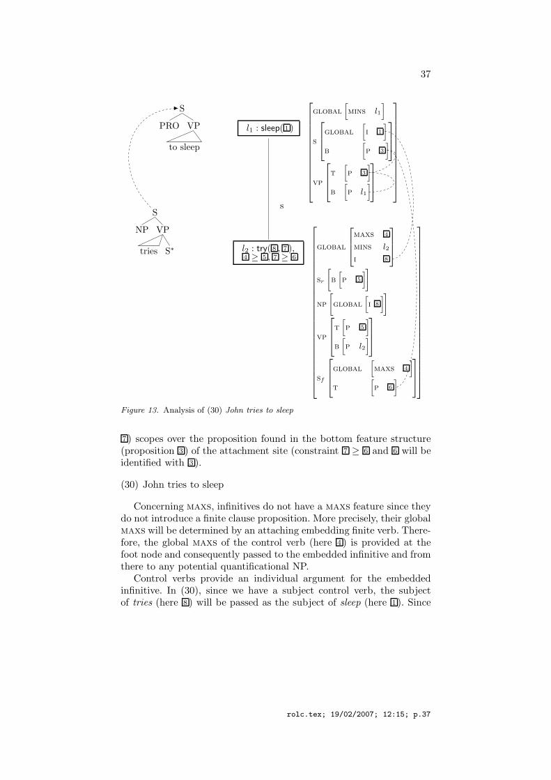
37

S

PRO VP

to sleep

l1 : sleep( 1 )

global[

mins l1

]

s

global[

i 1

]

b[

p 3

]

vp

t[

p 3

]

b[

p l1

]

sS

NP VP

tries S∗ l2 : try( 8 , 7 ),4 ≥ 5 , 7 ≥ 6

global

maxs 4

mins l2

i 8

sr

[

b[

p 5

]

]

np

[

global[

i 8

]

]

vp

t[

p 5

]

b[

p l2

]

sf

global[

maxs 4

]

t[

p 6

]

Figure 13. Analysis of (30) John tries to sleep

7 ) scopes over the proposition found in the bottom feature structure(proposition 3 ) of the attachment site (constraint 7 ≥ 6 and 6 will beidentified with 3 ).

(30) John tries to sleep

Concerning maxs, infinitives do not have a maxs feature since theydo not introduce a finite clause proposition. More precisely, their globalmaxs will be determined by an attaching embedding finite verb. There-fore, the global maxs of the control verb (here 4 ) is provided at thefoot node and consequently passed to the embedded infinitive and fromthere to any potential quantificational NP.

Control verbs provide an individual argument for the embeddedinfinitive. In (30), since we have a subject control verb, the subjectof tries (here 8 ) will be passed as the subject of sleep (here 1 ). Since

rolc.tex; 19/02/2007; 12:15; p.37

38

S

NP VP

laughs

l1 : laugh(j),1 ≥ 2

global

[

maxs 1

mins l1

]

s

[

b[

p 2

]

]

vp

t[

p 2

]

b[

p l1

]

s

S

NP VP

thinks S∗

l2 : think(m, 3 ),4 ≥ 5 , 3 ≥ 6

global

[

maxs 4

mins l2

]

sr

[

b[

p 5

]

]

vp

t[

p 5

]

b[

p l2

]

sf

[

global[

maxs 6

]

]

Figure 14. Analysis of (32)

the control verb provides this individual argument, we take it to be itsglobal feature i. The infinitive requests for this global feature at the Snode where the embedding finite verb will adjoin and identifies it withits individual argument.

In the case of an object control verb as in (31) the object is providedto the infinitive as argument.

(31) John forces Mary to come

4.5. Attitude verbs

Syntactically, attitude verbs resemble control verbs, i.e., their ele-mentary trees look similar. See for example the elementary trees for(32) in Fig. 14.

(32) Mary thinks John laughs

The analysis of attitude verbs such as thinks in (32) is shown inFig. 14. Attitude verbs, in contrast to control verbs, take a finite clause

rolc.tex; 19/02/2007; 12:15; p.38

39

as their argument. This means that the embedded finite verb specifies amaxs and that the attitude verb will be able to operate over it and thusblock scope. The difference between the two types of verbs is modelledin the following way: whereas the complement of a control verb mustscope over the relevant p value of the embedded verb ( 7 ≥ 6 in Fig. 13),the complement of an attitude verb must scope over the maxs of theembedded verb ( 3 ≥ 6 in Fig. 14). In Fig. 14, the foot node of thethinks tree is the argument position for the embedded sentence. Atthis node we place a request for the embedded maxs (here 6 ). Theadjunction then leads to the unification 6 = 1 .

This analysis means that quantifiers attaching to the lower verbcan scope over tries but not over thinks. E.g., in (33), wide scope ofeverybody is excluded.

(33) Mary thinks John likes everybody

Now we have seen enough to be able to analyze another missing linkexample from section 2, namely (34) where we have an attitude verband, additionally, a raising verb or adverb in the embedded sentence.

(34) a. Mary claims John seems to laughb. Mary claims John apparently laughs

In general, by unification, in a finite clause, the proposition intro-duced by the topmost adverb/raising verb is the p value of the rootof the verb tree which is below the maxs proposition. Since attitudeverbs as claim embed the maxs of their argument, they necessarily takescope over any embedded raising verb/adverb. The analysis of (34b) isshown in Fig. 15.

4.6. Nested quantificational NPs

Now we will consider examples such as (21), repeated in (35) with threequantificational NPs where two of them are nested.

(35) Two policemen spy on someone from every city.

As mentioned above, (35) has only four possible scope orders out offive:

(36)a. 2 > ∃ > ∀ b. ∃ > ∀,2

c. 2 > ∀ > ∃ d. ∀ > ∃ > 2 e. * ∀ > 2 > ∃

rolc.tex; 19/02/2007; 12:15; p.39

40

l1 : laugh(j), 1 ≥ 2

global

[

maxs 1

mins l1

]

s

[

b[

p 2

]

]

vp

t[

p 2

]

b[

p l1

]

s vp

l2 : claim(m, 3 ),4 ≥ 5 , 3 ≥ 6

l3 : apparently( 7 ),7 ≥ 8

global

[

maxs 4

mins l2

]

sr

[

b[

p 5

]

]

vp

t[

p 5

]

b[

p l2

]

sf

[

global[

maxs 6

]

]

r

[

b[

p l3

]

]

f

[

t[

p 8

]

]

Figure 15. Analysis of (34b)

The question is how to derive an underspecified representation thatallows for the readings (36a-d) and excludes reading (36e).

Joshi et al. (2003) propose to derive the specific scope constraintsfor such constructions –namely, the fact that the third quantificationalNP cannot scopally intervene between the host and nested quantifiers–from the way the scope parts of the different quantifiers combine. Thisaccount is not possible if the scope part is not separated from the NPtree carrying the lexical material.

In the following we will show that the desired constraints can be ob-tained without multicomponents if we use the scope constraint languagewe have so far.29

29 Readings (b’) and (b”) from footnote 25 –* ∃ > ∀ > 2 and * ∃ > 2 > ∀respectively– are excluded on independent grounds, since they do not yield tree-shaped terms: Assume that the three quantifiers are l2 : 2(x, 3 , 4 ), l4 : some(y, 7 , 8 )and l8 : every(z, 13 , 14 ). Then for the scope order some > 2 and some > every wehave the following: 2 is in the nuclear scope of some, i.e., 8 ≥ l2 because of spy

being in the nuclear scope of both, some and 2. The proposition coming with from

rolc.tex; 19/02/2007; 12:15; p.40

41

S

NP VP

spy NP

NP

two policemen

NP

Det N

some -one

N

N∗ PP

P NP

from

NP

every city

Figure 16. Derivation for (35)

To exclude the reading every > 2 > some, the idea, in a nutshell,is the follwoing. We derive a constraint saying that the maximal nu-clear scope of every is the some proposition. This means that every canrise and take scope over some, but, if it does so, then it has to takeimmediate scope over some.

The analysis of (35) is shown in Fig. 16 and Fig. 17. The new maxsvalue for the maximal scope of embedded quantifiers is the global maxsof the from tree. It is equated with the label of the quantifier to whichfrom attaches. Consequently, any quantifier attaching to from (hereevery) takes the label of this quantifier as its limit for maximal scope.Quantifiers now provide their labels as potential global maxs at theirN nodes in case something adjoins here. Modifiers such as from receivethis value then as the global maxs that limits the nuclear scope offurther embedded quantifiers. In our example, the maximal nuclearscope of every (here 15 ) will be equated with the global maxs of from(here 12 ), which in turn is equated with l4. For every, we consequentlyobtain l4 ≥ 14 .

The result of the semantic unifications in Fig. 17 is the semanticrepresentation (37):

must of course be in the restriction of some and it must be in the nuclear scope ofevery. Consequently, if every is in the scope of some, it must be in its restriction,i.e., 7 ≥ l8. Then, if 2 > every, with 8 ≥ l2 (2 in the nuclear scope of some), every

would have to be at the same time in the nuclear scope of some, i.e., 8 ≥ l8. Thiswould violate the assumed principle that terms are tree-shaped, i.e., that nothingis part of two different arguments of the same predicate (here every cannot be partof 7 and 8 at the same time). Similarly, if every > 2, then 2 would be at the sametime in the restriction and the nuclear scope of some, leading to the same problem.

rolc.tex; 19/02/2007; 12:15; p.41

42

l1 : spy(x, y),1 ≥ l1

[

global

[

maxs 1

mins l1

]]

np1 np2

l2 : 2(x, 3 , 4 ),l3 : policeman(x)3 ≥ l3,5 ≥ 4 , 4 ≥ 6

l4 : some(y, 7 , 8 ),l5 : person(y)7 ≥ 11 ,9 ≥ 8 , 8 ≥ 10

[

np

[

global

[

maxs 5

mins 6

]

]]

np

[

global

[

maxs 9

mins 10

]

]

n

global[

maxs l4

]

t[

p 11

]

b[

p l5

]

n

l6 : 17 ∧ 18 , l7 : from(y, z),17 ≥ 19 , 18 ≥ l7

global

[

maxs 12

mins l7

]

nr

[

b[

p l6

]

]

nf

[

t[

p 19

]

]

np

l8 : every(z, 13 , 14 ),l9 : city(z)13 ≥ l9,15 ≥ 14 , 14 ≥ 16

[

np

[

global

[

maxs 15

mins 16

]

]]

Figure 17. Semantic analysis of (35)

rolc.tex; 19/02/2007; 12:15; p.42

43

(37)

l1 : spy(x, y), l2 : 2(x, 3 , 4 ), l3 : policeman(x)

l4 : some(y, 7 , 8 ), l6 : 17 ∧ 18 , l5 : person(y), l7 : from(y, z)

l8 : every(z, 13 , 14 ), l9 : city(z)

1 ≥ l1, 3 ≥ l3, 1 ≥ 4 , 4 ≥ l1, 7 ≥ l6, 1 ≥ 8 , 8 ≥ l117 ≥ l5, 18 ≥ l7, 13 ≥ l9, l4 ≥ 14 , 14 ≥ l7

As desired the scope order every > 2 > some is not possible: Assumeit was possible, i.e., l8 > l2 > l4. Then with 14 ≥ l7 and l8 > l4 > 7 ≥l6 > 18 ≥ l7, it follows that 14 ≥ l2 and 14 ≥ l4. Consequently thedisambiguation δ would be such that 13 → l9, 14 → l2, 3 → l3, 4 →l4, 7 → l6, 8 → l1, 17 → l5, 18 → l7. But then δ( 14 ) = l2 > δ( 4 ) = l4.This contradicts the constraint l4 ≥ 14 .

In order to obtain the underspecified representation (37), we haveto allow scope constraints that do not correspond to normal dominanceconstraints since we need a constraint of the form l ≥ x where l is alabel, x a meta-variable. As already mentioned, with some restrictionson these constraints, they could probably be integrated into the con-straint solver for dominance constraints so that polynomial constraintsolving is still possible. It is an important result that it is enough tohave only a slight extension of normal dominance constraints in orderto capture the scope relations in nested quantifiers. In particular, theoriginal constraint language allowing only subordination constraintsdoes not need to be extended in the style of the quantifier sets proposedby Joshi et al. (2003).30

30 Following Larson (1987), the main concern in the literature on nested NPs hasbeen to rule out the reading (21e) where another quantifier scopally intervenes be-tween the host and the nested quantifier. However, more recently, Sauerland (2000)has presented data suggesting that intervention is possible if the extra quantifier isnot an NP itself but a verbal element (e.g. want), as in (38). We presently do not havean account for why this difference results (but see Joshi et al. 2003). However, notethat the relaxation of scope constraints with verbal intervenors seems to be a widerphenomenon independent of the nested NPs at hand. In (39), e.g., someone cannotscope under the verbal conjunction, but it can scope under it if some intensionalverbal element intervenes, as in (40).

(38) John wants to meet someone from every city you do (want to meet someonefrom).

(39) Someone from NY jumped and ran.* ∃x[from(x,ny) ∧ jumped(x)] ∧ ∃y[from(y, ny) ∧ ran(y)]

(40) Someone from NY is likely to win the lottery but unlikely to win this bet.likely(∃x[from(x,ny) ∧ win(x, l)]) ∧ unlikely(∃y[from(y, ny) ∧ win(y, b)])

rolc.tex; 19/02/2007; 12:15; p.43

44

5. Situation Binding in LTAG

5.1. Theoretical Background

Independently of LTAG or any other grammar formalism, in orderto represent the semantics of natural language, a formal language isneeded that allows us to evaluate linguistic expressions not only at theactual situation or world but also at other logically possible worlds.In this subsection, we will describe two formal languages that havebeen traditionally used for this purpose in the literature, namely ModalPredicate Logic (ModPrL) –without situation terms– and Two-SortedType Theory (Ty2) –with situation terms and quantification over them.Then we will summarize Cresswell’s (1990) argument in favor of Ty2.Because of this argument, the formal language assumed in the presentpaper and defined in section 3.1 follows Ty2 rather than ModPrL, thatis, it includes situation variables and direct quantification over them.

A simple example of intensional language is Modal Predicate Logic.ModPrL is like standard Predicate Logic with the addition of the syn-categorematic symbols 2 and 3. For a model M of the sort describedin (41) and an assignment function g from variables to individuals inM , the interpretation of terms and formulas is defined in (42) and (43)(see Gamut, 1991: vol. II, ch 3.).

(41) A model M for a modal predicate logic language L consists of:

i. a non empty set of possible worlds W

ii. an accessibility relation R on W 31

iii. a domain function assigning a domain of individuals Dw

to each w ∈ W

iv. an interpretation function I such that:

a. I assigns an entity I(c) to each constant c of L, and

b. for every world w ∈ W, I assigns a subset Iw(P) of(Dw)n to each n-ary predicate letter P of L.

31 R can stand for the epistemic (Epi, e.g. with know), deontic (Deo, e.g. withhave to), doxastic (Dox, e.g. with believe), etc. accessibility relation. wRw′ is readas ‘w′ is accessible from w’. E.g., wEpiw′ is read as ‘w′ is epistemically accessiblefrom w’, that is, ‘for all we know in the actual world w, w′ could equal w’.

rolc.tex; 19/02/2007; 12:15; p.44

45

(42) Interpretation of terms:32 [[t]]M,w,g

1. If t is a constant,

[[t]]M,w,g = I(t) if I(t) ∈ Dw (and undefined otherwise).

2. If t is a variable,

[[t]]M,w,g = g(t) if g(t) ∈ Dw (and undefined otherwise).

(43) Interpretation of formulas: [[φ]]M,w,g

3. [[P (t1, ..., tn)]]M,w,g = 1

iff 〈[[t1]]M,w,g,...,[[tn]]M,w,g〉 ∈ [[P ]]M,w,g

4. [[¬φ]]M,w,g = 1 iff [[φ]]M,w,g = 0

5.1. [[φ ∧ ψ]]M,w,g = 1 iff [[φ]]M,w,g = [[ψ]]M,w,g = 1

5.2. ...

6.1. [[∀x[φ]]]M,w,g = 1 iff for all d ∈ Dw: [[φ]]M,w,gd/x= 1

6.2. [[∃x[φ]]]M,w,g = 1 iff for some d ∈ Dw: [[φ]]M,w,gd/x= 1

7.1. [[2[φ]]]M,w,g = 1 iff for all w′ such that wRw′:[[φ]]M,w′,g=1

7.2. [[3[φ]]]M,w,g = 1 iff for some w′ such that wRw′:[[φ]]M,w′,g = 1

To see an example, the sentence (44) is translated into ModPrL asin (45) for its reading ‘It must be the case that someone or other fromNew York wins the lottery’.

(44) Someone from NY must have won the lottery.

(45) 2[∃x[person(x) ∧ from(x, ny) ∧ win(x)]

An alternative to intensional languages like ModPrL is the so-calledTwo-Sorted Type Theory (Ty2) (Gallin, 1975:58-63). Ty2 is character-ized by having two sorts of basic individuals rather than one: besidesregular individuals (type e), we add possible situations or worlds as abasic type (type s). This means that a Ty2 (first-order) formal languagewill include variables over worlds, and that these world variables willserve as arguments of predicates and will combine with the syncate-gorematic symbols ∀ and ∃. The interpretation is defined in (47)-(48).A Ty2 version of ModPrL assigns the translation (49) to the aforemen-tioned reading of (44) –with must interpreted at world w0–, with directquantification over world variables.

32 Here we slightly deviate from Gamut (1991). In the end, though, in both casesthe condition that I(t) and g(t) ∈ Dw ends up as a presupposition rather than aspart of the assertion.

rolc.tex; 19/02/2007; 12:15; p.45

46

(46) A model M for the Ty2 version of modal predicate logic languageL consists of:i. a non empty set of individuals De,

ii. a non-empty set of possible worlds Ds

iii. an accesibility relation R on Ds

iv. an interpretation function I such that:

a. I assigns an entity I(c) to each constant c of L, and

b. I assigns a subset I(P) of De,1 ×...× De,n× Ds to eachn-ary predicate letter P of L.

(47) Interpretation of terms: [[t]]M,g

1. If t is a constant, [[t]]M,g = I(t).

2. If t is a variable, [[t]]M,g = g(t).

(48) Interpretation of formulas: [[φ]]M,g

3. [[P (t1, ..., tn, w)]]M,g = 1

iff 〈[[t1]]M,g,...,[[tn]]M,g, [[w]]M,g〉 ∈ [[P ]]M,g

4. [[¬φ]]M,g = 1 iff [[φ]]M,g = 0

5.1. [[φ ∧ ψ]]M,g = 1 iff [[φ]]M,g = [[ψ]]M,g = 1

5.2. ...

For any variable v of type e or s:

6.1. [[ ∀v[φ] ]]M,g = 1 iff for all d ∈ De∪Dw: [[φ]]M,gd/v= 1

6.2. [[ ∃v[φ] ]]M,g = 1 iff for some d ∈ De∪Dw: [[φ]]M,gd/v=1

(49) ∀w′ [ w0Rw′ → ∃x[person(x,w′) ∧ from(x, ny,w′) ∧ win(x,w′)] ]

Note that a Ty2 language has more expressive power than ModPrL,as the former, but not the latter, will allow for a predicate within thescope of a modal to be evaluated at a higher world w. For (44) e.g., Ty2will allow for the truth conditions in (50) –where the complex predicate-one from NY is in the scope of the modal but evaluated at the actualworld w0–, but standard ModPrL will not generate this reading.

(50) ∀w′ [ w0Rw′ → ∃x[person(x,w0) ∧ from(x, ny,w0) ∧ win(x,w′)] ]

This means that the scope and the situation binding of a predicate(e.g. a noun, adjective, verb, preposition, etc.) are two different issuesin Ty2 but necessarily go together in standard ModPrL: in the former,a predicate within the scope of several intensional operators can beevaluated at the world w introduced by any of these operators; in the

rolc.tex; 19/02/2007; 12:15; p.46

47

latter, it will necessarily be evaluated at the world introduced by theclosest of these operators. The crucial question is, then, whether scopeand situation binding of a predicate go together in natural language–as in ModPrL– or not –as in Ty2.

The empirical observation for natural language is that not all thepredicates under the scope of a given intensional operator (e.g. must,if, to rumour) are evaluated at the w′ introduced by that operator. Forexample, in the most salient reading of (51), every and thus its restrictorpoor child scope under if, but still poor child denotes the set of actualpoor children rather than the set of poor children in the hypotheticalworld.33 In a similar fashion, in (52), every scopes under the secondif but its restrictor poor child in the neighborhood is evaluated at theworld introduced by rumour.

(51) If every poor child was rich instead, this would be a happy world.

(52) I know there aren’t any poor children in this neighborhood.But, if there were poor children in this neighborhood, peoplewould rumour that if every poor child in the neighborhood wasrich instead, the mayor would be re-elected.

To capture all the possible world binding readings in natural lan-guage, we would need a switch operator actuallyn for every worldbinder in the sentence. Cresswell (1990) proves that a formal languagewith such switch operators has the expressive power of explicit quan-tification over world variables, that is, the power of a Ty2 language(Cresswell ,1990:ch 4). Ty2 gives us the translation of (51) in (53).

(53) ∀w [ w0Rw ∧ ∀x[poor-child(x,w0) → rich(x,w)]→ happy-world(this, w) ]

Hence, following Gallin (1975) and Cresswell (1990), our formal lan-guage defined in section 3.1 follows Ty2: each predicate has a worldargument and we explicitly quantify over world variables.

5.2. The Data

The punchline from the previous subsection is that scope and world orsituation binding are two separate phenomena in natural language. Asa consequence, a formal language with the expressive power of Ty2 is

33 If poor child in (51) was evaluated in the hypothetical world w′ introduced byif, w′ would have the contradictory property of being such that all the children thatare poor in w′ are rich in w′. This is clearly not the intended reading.

rolc.tex; 19/02/2007; 12:15; p.47

48

needed. Section 4 was concerned with handling scope data. Now thatwe have motivated the Ty2-like formal language we use, the presentsection tackles situation binding.

The empirical generalizations for situation binding in natural lan-guage are the following:

• Noun Phrases: The situation variable of an NP can be non-locally bound by a distant operator (Cresswell, 1990) (Farkas, 1997)(Percus, 2000) or remain free.

• Quantificational elements attached to the VP-spine: The situationvariable of material attached to the VP spine must be locally boundby the closest situation binder scoping over it (Percus, 2000). If thereis no situation binder scoping over it at all, then it remains free.

When a situation variable remains free, it defaults to the actualsituation s0.

Data supporting the first generalization are (51)-(52) in the previoussubsection. To see the different situation binding possibilities for NPsand VP-spine material, consider now sentence (54).

(54) Mary thinks that, in yesterday’s game, John sometimes beat thewinner.

Consider, furthermore, a scenario with s0 as the actual situation, s asthe situation consisting of yesterday’s entire game according to Mary’sbeliefs and several subsituations s′ corresponding to different rounds ofthat game in Mary’s beliefs. With this scenario in mind, (54) can beunderstood as having the winner translated as ιx[winner(x, s0)] (‘Of theactual overall winner x, Mary thinks that John beat x in some rounds’)or as ιx[winner(x, s)] (‘Mary thinks that in some rounds John beatwhoever the overall winner of the game in Mary’s beliefs is’), skippingin both cases over the local situation binder ∃s′. This is represented in(55). (The translation ιx[winner(x, s′)] is in principle possible as well,but having s′ for the winner and for beat is obviously pragmaticallydeviant.)

(55) ∀s [ s ∈ Doxm(s0) ∧ game(s) →∃s′[s′ ⊑ s∧ beat(j, ιx[winner(x, s0/s/#s

′)], s′)] ]‘Mary thinks that in some rounds John beat the actual overallwinner of the game / whoever the overall winner of the game is inMary’s belief worlds.’

In contrast, the situation variable of the verb beat must be locallybound by the ∃s′-quantifier of sometimes, yielding the subformulabeat(j, ιx[...], s′) that we see in (55). If it could be distantly bound

rolc.tex; 19/02/2007; 12:15; p.48

49

and represented as beat(j, ιx[...], s), as in (56), the sentence (54) wouldbe predicted to have a reading ‘Mary thinks John beat a sometimeswinner’, contrary to fact.

(56) ∀s [ s ∈ Doxm(s0) ∧ game(s) →∃s′[s′ ⊑ s∧ beat(j, ιx[winner(x, s′)], s)] ]‘Mary thinks John beat in the overall game the winner of someround.’

Furthermore, the (non-quantified) situation within sometimes must belocally bound by the ∀s-quantification of think, yielding the subformula∃s′[s′ ⊑ s] we see in (55). If it could be distantly bound and representedas ∃s′[s′ ⊑ s0], as in (57), the sentence would be able to roughly mean‘For every person that Mary thinks may be the overall winner, Johnsometimes beat that person’, again contrary to fact.34

(57) ∀s [ s ∈ Doxm(s0) ∧ game(s) →∃s′[s′ ⊑ s0∧ beat(j, ιx[winner(x, s)], s′)] ]‘For every person x that Mary thinks may be the overall winner,John beat x in some round.’

In sum, for NPs, situation binding is not determined by their surfacesyntax: their situation can be bound at any distance and, if unbound,it defaults to s0. For quantificational elements on the VP-spine, situa-tion binding is fully determined by the surface syntax: their situationvariable is bound by the closest situation binder and, if no such binderexists, it defaults to s0.

5.3. The analysis

In the same way that situation or world variables were added as anextra argument to each predicate in Ty2, we add situation variabless0, s, s

′, s′′, etc., situation meta-variables, and the feature s to ourLTAG semantic representations and semantic feature structures. Otherarguments –e.g agents, patients, goals, etc.– are linked to leaf nodesin the elementary tree, as they get their values from the substitutionsthat will be perfomed at those nodes. The situation argument is linkedto the VP-spine, as it can get its value from quantificational elementsadjoined to VP or to S. Since the situation argument of a verb can beaccessed from these two nodes but it can possibly only be bound once,it will be given two meta-variables in the semantic feature structure:

34 The expression Doxm(s0) stands for the set of doxastic alternatives of Maryin s0, i.e. the set of possible situations s that conform to Mary’s beliefs in s0. ⊑denotes the part-of relation between situations, as defined in Kratzer’s (1989).

rolc.tex; 19/02/2007; 12:15; p.49

50

a ‘lower’ one for VP-adjunctions and a ‘higher’ one for S-adjunctions,the latter being coindexed with the situation meta-variable in the toppart of the VP-node. This is illustrated in the feature structure for winin Fig. 18 (see 2 and 3 ).

The feature unification mechanism used for scope derives the situ-ation data as well. On the one hand, material attached to the verbalspine will unify its situation variables univocally with the situation vari-ables at the attachment positions. On the other hand, NPs will remainunderspecified with respect to situation binding. Since we saw that thebinder of an NP’s situation can be outside the closest finite clause,we impose no minimality or maximality constraints on NP situations,hence leaving NP situation binding completely underspecified.

(58) Mary thinks every person sometimes won.

This is illustrated in (58), where an attitude verb, a VP-adverb andan embedded quantifier interact for scope and for situation binding.The derivation is in Fig. 18. VP-attachment of sometimes -label l2-guarantees that it will quantify over the ‘lower’ situation variable 2 ofwin. Note that 2 is the situation argument in the formula l1 : win( 1 , 2 )in the semantic representation. S-attachment of think secures thatthinks will quantify over the ‘higher’ situation variable 3 in the featurestructure of win. Since by top-bottom unification 3 will be equatedwith the situation meta-variable 6 of sometimes, think will end upquantifying over the situation variable of sometimes. (If no adjunctionhad been perfomed at VP, by top-bottom unification, 3 would havebeen equated with 2 and thus thinks would have directly quantifiedover the situation of win.) As for the NP every person (or everyonefrom NY), no restrictions are placed on the situation variable 13 ofits restrictor proposition l3 : person(x, 13 ): 13 can be bound by anysituation binder scoping over it and, if unbound, it will default to s0.

One obtains the feature value identities 1 = x, 2 = s′, 8 = l1,4 = l2, 3 = 6 , 3 = s, 12 = l1, and 11 = 0 = 17 , which leads to (59):

(59)

l1 : win(x, s′), l2 : some(s′, s′ ⊑ s, 5 ), l3 : every(x, 9 , 10 ),

l4 : person(x, 13 ), l5 : every(s, s ∈ Doxm( 14 ), 15 )

16 ≥ l5, 15 ≥ 0 , 0 ≥ l2, 5 ≥ l1, 9 ≥ l4, 10 ≥ l1, 0 ≥ 10

In (59), the maximal scope of the quantificational NP is blocked bythe argument of thinks: the constraints 15 ≥ 0 and 0 ≥ 10 guaranteethat the argument 15 of thinks will include the nuclear scope 10 ofevery and thus scope over the entire l3 : every(x, 9 , 10 ). But the orderof the quantificational NP and the adverb is unspecified. The situation

rolc.tex; 19/02/2007; 12:15; p.50

51

l1 : win( 1 , 2 )0 ≥ 4

global

[

maxs 0

mins l1

]

s

[

b

[

p 4

s 3

]]

vp

t

[

p 4

s 3

]

b

[

p l1

s 2

]

np1

[

global[

i 1

]

]

s vp np1

l3 : every(x, 9 , 10 ),l4 : person(x, 13 ),9 ≥ l4, 10 ≥ 12 ,11 ≥ 10

global[

i x]

np2

[

global

[

maxs 11

mins 12

]

]

l5 : every(s, s ∈ Doxm( 14 ), 15 ),16 ≥ l5, 15 ≥ 17

global[

maxs 16

]

sr

[

b

[

p l5

s 14

]

]

sf

global[

maxs 17

]

t[

s s]

l2 : some(s′, s′ ⊑ 6 , 5 ),5 ≥ 8

vpr

[

b

[

p l2

s 6

]

]

vpf

[

t

[

p 8

s s’

]

]

Figure 18. Analysis of (58) Mary thinks everybody sometimes won with s featureidentifications.

rolc.tex; 19/02/2007; 12:15; p.51

52

14 in the l5 of thinks will default to s0, since there is no possible binderabove it and it will thus remain unbound. The situation variable 13 inl4 corresponding to the noun in every person is underspecified. It couldbe resolved to s0, to s, or –if every person is in the scope of sometimes,as in (60b)– also to s′. Consequently, one obtains the readings in (60):

(60) a. every(s, s ∈ Doxm(s0),every(x, person(x, 13 ), some(s′, s′ ⊑ s,win(x, s′))))

b. every(s, s ∈ Doxm(s0),some(s′, s′ ⊑ s, every(x, person(x, 13 ),win(x, s′))))

6. Comparison to other approaches outside LTAG

Besides LTAG, substantial work on quantifier scope has been done inseveral other grammar formalisms. We will point out some of themand briefly describe how they differ from the approach proposed in thispaper.

In the Generative Transformational Grammar framework, longdistance dependencies are captured by movement operations like Quan-tifier Raising (QR) (May, 1977) and wh-movement (Chomsky, 1986).These movement operations unambiguously determine the scope ofthe moved quantificational element. For example, for (61a), the longermovement of the NP every professor in (61b) univocally leads to thescope every > refused, whereas the shorter movement in (61c) resultsin the scope relation refused > every.35 More recently, movement hasbeen remodeled using Copy Theory in Chomsky’s (1995) MinimalistProgram: movement amounts to leaving copies of the “moved” elementin several syntactic positions. Only part of those copies is interpreted:the interpreted copy of the determiner gives the scope, while the in-terpreted copy of NP-part stays in situ. This is illustrated in (61b’,c’).This way of syntactically splitting the purely quantificational part fromthe NP-part in Minimalism is reminiscent of multicomponents in TAG(Joshi and Vijay-Shanker, 1999, Kallmeyer and Joshi, 2003) and of thedistinction between maxs and the rest of the semantics of the quantifierin this paper.

(61) a. John refused to meet every professorb. [S [every professor]1 [S John refused to meet t1] ]c. [S John refused [S [every professor]1 to meet t1] ]

35 See May (1985), Aoun and Li (1993), and Kitahara (1996) among others for avariant where QR still leads to ambiguity.

rolc.tex; 19/02/2007; 12:15; p.52

53

b’. [S every professor [S John refused to meet every professor] ]c’. [S John refused [S every professor to meet every professor] ]

Some important differences between Transformational Grammarand the present LTAG proposal are the following. First, it is not clearhow to build the desired locality conditions of quantifier dependenciesinto the definition of QR and islands for QR. It is intuitive to defineQR as being able to cross certain boundaries (namely, non-finite clauseboundaries, in case (ii)) and not others (finite clause boundaries, incase (i)). But it is not clear why, after being allowed to cross a givenboundary (a host NP, in case (iii)), the quantifier should be requiredto stop rising. That is, if every city is allowed to rise outside the hostNP and attach to S2 in (64a), it is not clear why the quantifier is notable to attach to S1 in (64b).36

(64) Two politicians spy on someone from every city.a. [S [two politicians]1 [S [every city]3 [S [someone from t3]2 [S t1

spy t2 ] ] ] ]b. [S [every city]3 [S [two politicians]1 [S [someone from t3]2 [S t1

spy t2 ] ] ] ]

In contrast, in the proposed LTAG framework, the maximal scopewindow is not determined by movement and islands to that movement,but by what maxs is equated with. If the maxs of the quantificationalNP is identified with the maxs of the higher predicate Q, this meansQ lets NP-scope pass. If the maxs of NP is equated with somethinginside the complement of Q, then Q blocks NP-scope. If the maxsof NP is equated with the label of Q itself, this guarantees that theNP can scope immediately over Q but not any higher. In sum, in ourapproach, locality conditions on NP-scope correlate with the featureidentifications that an embedding operator Q can possibly perform.

Second, despite some resemblance between Copy Theory and ourseparation between maxs and the rest, the two approaches differ in

36 In fact, some treatments of inverse linking in the Transformational Grammarframework involve QRing the nested NP not to the S node but to the edge of thehost NP, as in (62). But then something else needs to be done for the nested NPevery city in (63) to be able to scope over the rest of the sentence and bind thepronoun its. See May (1985), Heim and Kratzer (1998), Buring (2001) for somepossibilities.

(62) [S ([two politicians]1) [NP [every city]3 [ someone from t3 ] ]2 ([twopoliticians]1) t1 spy t2 ]

(63) Someone from every cityi hates itsi subway system.

rolc.tex; 19/02/2007; 12:15; p.53

54

important respects. One difference is that the scope part determinesthe exact scope in Copy Theory but maxs gives the maximal possiblescope in LTAG. Another difference is that special semantics is neededto interpret split quantificational phrases in Copy Theory. For example,if we interpret the structure (66b) as in (66c), the truth conditions aretoo weak: any x that is not a professor would make the subformulaunder “For most x” true, and thus, if there are more non-professorsthan professors, the entire (66c) becomes automatically true regardlessof whether John has seen most professors or not. Special semantics havebeen developed for the split structures proposed in Copy Theory.37 Inthe proposed LTAG approach, instead, the semantic contribution of theNP-part always ends up in the restrictor of the quantifier and never inits nuclear scope, regardless of what happens with maxs, and thus theinterpretive problem in (66) does not arise.

(66) a. John hasn’t seen (yet) most professors.b. [ mostx professors [ John hasn’t seen most professorsx] ]c. “For most x: ¬[see(j, x) ∧ professor(x)]”

Third and finally, recall that the scope and the situation variableof a given NP do not need to go together. Once a Ty2 language withsituation variables is assumed, nothing predicts the asymmetry betweensituation variables on the verbal spine and situation variables in NPsif we do Montague-style semantics on the derived tree. As argued inPercus’ (2000), a situation binder –e.g. the λ-abstractor under if in(51)– will simply look for a situation variable in its sister node –theentire [every poor child was rich]– without knowing the internal struc-ture of that sister, that is, without knowing what situation variablebelongs to the verbal predicate and which to the NP. In fact, Percussuggests that the appropriate binding conditions for situation variablesin Transformational Grammar need to be stated in the syntax. In thepresent LTAG proposal, constraints on situation binding follow fromthe semantic s features and the architecture of the derivation tree.Situation binders like think, sometimes or if attach to the verb tree

37 Besides Copy Theory, split structures have been proposed because of exampleslike (65) (Reinhart, 1992), in which the wh-phrase which phantasies about himselfis understood with matrix scope but its restrictor contains a variable bound withinthe embedded clause. See Reinhart (1992) and Romero (1998) for choice functionsfor wh-phrases, Rullmann and Beck (1998) for a presuppositional treatment of wh-phrases, and Fox (1999) for quantificational NPs.

(65) a. Who knows which patienti has [which phantasies about himselfi]?b. [ whox whichy phantasies about himself [ x knows which patientz has whichphantasiesy about z ] ]

rolc.tex; 19/02/2007; 12:15; p.54

55

and hence ask the verb for a situation variable. Together with theconstraints on scope, this forces local binding of situations on the verbalspine. The same situation binders do not combine with the NP, andhence cannot ask the NP for a situation to bind. As a result, binding ofNP situation variables by VP-spine material is not enforced and, thus,they remain underspecified.38

In the Combinatory Categorial Grammar (CCG) framework, Steed-man (2003) has proposed an extensive theory of quantifier scope. CCGis a system where lexical entries encode syntactic and semantic types.Larger structures are built by applying different rules, allowing typeshifting in the semantics. In contrast to our approach, quantifier scopedepends on the order in which quantifiers and certain operations apply,and the interpretations one obtains are not underspecified with respectto scope. Steedman treats only universals every, each and no as truegeneralized quantifiers. All other quantificational determiners –e.g. two,some, at most four, etc.– are explained as Skolem terms. A Skolem termdepends on any variable introduced by a true quantifier scoping over theSkolem term. But, crucially, the Skolem term can be applied at any timein the course of the derivation. I.e., if it is applied before the Skolemterm ends up in the scope of some quantifier, then the Skolem term doesnot depend on that quantifier and therefore appears to have wide scopewith respect to it. In a sentence containing only Skolem terms, a scopeorder effect can only be obtained through the distributivity operator,which introduces true universal quantification. As distributivity followssurface order, the subject is predicted to always have scope over theobject in this case, as in (67):

(67) Some linguist knows at most two languagessome > at most two; * at most two > some

While Steedman (2003) makes finer distinctions between quantifi-cational determiners than the ones aimed for in the present paper, webelieve that his account may prove too restrictive. By translating indef-inites exclusively as Skolem terms and never as generalized quantifiers,he can account for the unique surface scope of (67). But it is not clearwhether the model theory he sketches in his appendix can then derivethe correct truth conditions for the every > a reading of (68a). Notethat the truth conditions paraphrased in (68b) do not capture thisreading: they yield true even if no student that read a (any) paper by

38 Underspecification of NP situation variables behaves exactly like underspec-ification of other NP arguments, e.g. his in his cat. Both can be bound locally,non-locally, or simply remain unbound and default to some salient situation (s0) orindividual. See footnote 9.

rolc.tex; 19/02/2007; 12:15; p.55

56

Frege passed the class, as long as for each student there is a paper byFrege that that student did not read.39

(68) a. Every student that read a paper by Frege passed the class.b. There is a Skolem function fpaper−by−Frege such that:

∀x[student(x) ∧ read(x, fxpaper−by−Frege) → pass(x)]

Furthermore, in contrast to our approach, Steedman assumes quan-tifier scope not to be finite clause bound. We have referred the readerto analyses of apparent counterexamples to finite clause boundednessin footnote 25, p. 31.40

Other computational semantics approaches that show some similar-ities with our framework are approaches within Head-Driven PhraseStructure Grammar (HPSG) (Pollard and Sag, 1994), namely Mini-mal Recursion Semantics (MRS) (Copestake et al., 1999) and morerecently Lexical Resource Semantics (Richter and Sailer, 2004). Ofcourse, HPSG differs crucially from TAG: The grammar is a set ofconstraints that describe parts (finite subtrees) of the whole structure(in TAG terms, the derived tree). This means that there is no extendedlocality in the sense of TAG that allows to localize long dependencies.The underlying structures are typed feature structures that can bethought of as phrase structure trees with feature structures labelling thenodes. These features structures allow structure sharing and reentrancy.

For semantics, Copestake et al. (1997) use flat semantic representa-tions enriched with propositional meta-variables and scope constraints.However, the way they deal with quantifier scope is different from ourproposal and it is not clear how they obtain the various constraints forquantifier scope mentioned in this paper. The approach by Richter andSailer (2004) has a lot in common with our approach, despite the differ-ent formalism (see also Kallmeyer and Richter, 2006 for a comparison).Of course, since they do not have an extended domain of locality, theycompute semantics on the derived tree, i.e., the constituency structure,using general semantic principles to obtain scope constraints. But theyalso use a Ty2 language with underspecification and, particularly, theyhave features excont and incont that resemble very much to ourmaxs and mins: excont constitutes an upper boundary for the scope

39 This problem was noted in Chierchia’s (2001) for certain choice functionapproaches to indefinites.

40 Steedman (2003) also derives interesting scope constraints on coordinate struc-tures like (69). We refer the reader to Babko-Malaya (2004) for an LTAG analysisof coordination within the semantic framework in the present paper.

(69) Every boy admires and every girl detests some saxophonist.

rolc.tex; 19/02/2007; 12:15; p.56

57

of a quantifier. However, it still needs to be investigated in which casesexcont might be blocked and in which cases it might be passed up.incont corresponds to the lowest proposition and it constitutes theminimal nuclear scope of attaching quantifiers. Both excont and in-cont are passed up the constituency tree along the head projectionline. We take the striking similarity between excont and incont onthe one hand and our maxs and mins on the other hand as an additionalevidence for the adequacy of our proposal.

7. Conclusion

In this paper we have introduced an LTAG semantics framework basedon the derivation tree. Besides underspecified semantic representations,semantic feature structure descriptions are assigned to elementarytrees. As the semantic composition operation, we use conjunction ofthe feature descriptions plus additional feature value equations. Theseadditional equations are parallel to the unifications performed for thesyntactic features on the derived tree that are used in TAG.

Roughly, the semantic feature structure descriptions serve two pur-poses. On the one hand, they encode the contributions of the semanticrepresentations to functional applications. I.e., they state which elmentsare contributed as possible arguments for other semantic expressionsand which arguments need to be filled. They thereby simulate lambdaabstraction and functional application. On the other hand, they alsoserve to model the scopal behaviour of different operators and tocapture the different boundaries for scope.

Within this framework, we have proposed an account of the differ-ences between quantificational NPs on the one hand and quantifica-tional elements attached to the verbal spine (adverbs, raising verbs,attitude verbs, etc.) on the other hand with respect to their scopepossibilities and also with respect to the way their situation variablesare bound.

The main aspects of our analysis are the following: The scope ofquantificational NPs is limited by an upper and a lower boundary con-stituting a kind of scope window. These boundaries are global features,i.e., they depend on elementary trees but not on single nodes in ele-mentary trees. Within this window, the quantifier can scope freely. Thebinding of the situation variable of an NP does not depend on syntaxand therefore remains unspecified during the syntactic derivation; inthe disambiguation process, either it becomes a bound variable or itdefaults to s0. In contrast to this, quantificational elements on theverbal spine take scope where they attach making use of a local feature

rolc.tex; 19/02/2007; 12:15; p.57

58

specifying the proposition corresponding to the tree below a specificnode in the constituent structure. Furthermore, their situation binderalso depends on a local feature of the node they attach to, since theirbinder has to be the next higher binder on the verbal spine (if no binderis found, the situation defaults to s0 in the disambiguation).

The combination of LTAG’s extended domain of locality with a se-mantics using feature structure descriptions enables us to capture evenapparently non-local scope relations within a mildly context-sensitiveframework: The structures underlying the computation of syntax andsemantics are the context-free derivation trees.

References

Abeille, A.: 2002, Une grammaire electronique du francais. Paris: CNRS Editions.Aoun, J. and Y. A. Li: 1993, Syntax of Scope. MIT Press.Artstein, R.: 2003, ‘Quantificational arguments in temporal adjuncts clauses’. Ms.

Technion University.Babko-Malaya, O.: 2004, ‘LTAG Semantics of NP-Coordination’. In: Proceedings of

TAG+7. Vancouver.Bech, S. and H. Rullmann: 1999, ‘A Flexible Approach to Exhaustivity in Questions’.

Natural Language Semantics 7(3), 249–297.Berman, S.: 1991, ‘On the Semantics and Logical Form of Wh-Clauses’. Ph.D. thesis,

University of Massachusetts at Amherst.Blackburn, P. and E. Spaan: 1993, ‘A Modal Perspective on the Computational

Complexity of Attribute Value Grammar’. Journal of Logic, Language andInformation 2, 129–169.

Bos, J.: 1995, ‘Predicate Logic Unplugged’. In: P. Dekker and M. Stokhof (eds.):Proceedings of the 10th Amsterdam Colloquium. pp. 133–142.

Bouma, G., R. Malouf, and I. Sag: 1998, ‘Adjunct Scope’. Presented at the WorkshopModels of Underspecification and the Representation of Meaning, 18–22 May1998, Bad Teinach.

Buring, D.: 2001, ‘A Situation Semantics for Binding out of DP’. In: R. Hastings,B. Jackson, and Z. Zvolenski (eds.): Proceedings from Semantics and LinguisticTheory XI. Ithaca, pp. 56–75, CLC.

Candito, M.-H. and S. Kahane: 1998, ‘Can the TAG Derivation Tree represent aSemantic Graph? An Answer in the Light of Meaning-Text Theory’. In: FourthInternational Workshop on Tree Adjoining Grammars and Related Frameworks,IRCS Report 98–12. University of Pennsylvania, Philadelphia, pp. 25–28.

Chierchia, G.: 1993, ‘Questions with quantifiers’. Natural Language Semantics 1,181–234.

Chierchia, G.: 2001, ‘A puzzle about indefinites’. In: C. Cecchetto, G. Chierchia, andM. Guasti (eds.): Semantic Interfaces: reference, anaphora and aspect. Stanford:CSLI.

Chomsky, N.: 1986, Barriers. Cambridge, Mass.: MIT Press.Chomsky, N.: 1995, The Minimalist Program. MIT Press.Cinque, G.: 1999, Adverbs and functional heads : a cross-linguistic perspective. NY:

Oxford University Press.

rolc.tex; 19/02/2007; 12:15; p.58

59

Copestake, A., D. Flickinger, I. A. Sag, and C. Pollard: 1999, ‘Minimal RecursionSemantics. An Introduction’. Manuscript, Stanford University.

Cresswell, J. M.: 1990, Entities and Indices. Dordrecht: Kluwer.Dras, M., D. Chiang, and W. Schuler: 2004, ‘On Relations of Constituency and

Dependency Grammars’. Journal of Language and Computation 2(2), 281–305.Farkas, D.: 1997, ‘Evaluation Indices and Scope’. In: A. Szabolsci (ed.): Ways of

scope taking. Dordrecht: Kluwer.Forbes-Riley, K., B. Webber, and A. K. Joshi: To appear, ‘Computing Discourse

Semantics: The Predicate-Argument Semantics of Discourse Connectives in D-LTAG’. Journal of Semantics.

Fox, D.: 1999, Economy and Semantic Interpretation. MIT Press.Fox, D. and U. Sauerland: 1996, ‘Illusive Scope of Universal Quantifiers’. In:

Proceedings of NELS 26. Amherst.Frank, A. and J. van Genabith: 2001, ‘GlueTag. Linear Logic based Semantics for

LTAG – and what it teaches us about LFG and LTAG’. In: M. Butt and T. H.King (eds.): Proceedings of the LFG01 Conference. Hong Kong.

Frank, R.: 1992, ‘Syntactic Locality and Tree Adjoining Grammar: Grammat-ical, Acquisition and Processing Perspectives’. Ph.D. thesis, University ofPennsylvania.

Fuchss, R., A. Koller, J. Niehren, and S. Thater: 2004, ‘Minimal Recursion Se-mantics as Dominance Constraints: Translation, Evaluation, and Analysis’. In:Proceedings of the 42nd Annual Meeting of the Association for ComputationalLinguistics (ACL’04). Barcelona, Spain.

Gallin, D.: 1975, Intensional and Higher-Order Modal Logic with Applications toMontague Semantics, North Holland mathematics studies 19. Amsterdam:North-Holland Publ. Co.

Gamut, L.T.F.: 1991, Logic Language and Meaning. University of Chicago Press.Gardent, C. and L. Kallmeyer: 2003, ‘Semantic Construction in FTAG’. In:

Proceedings of EACL 2003. Budapest.Ginzburg, J. and I. A. Sag: 2000, Interrogative Investigations. The Form, Meaning,

and Use of English Interrogatives, No. 123 in CSLI Lecture Notes. CSLI.Heim, I. and A. Kratzer: 1998, Semantics in Generative Grammar. Blackwell.Hobbs, J. R. and S. M. Shieber: 1987, ‘An Algorithm for Generating Quantifier

Scopings’. Computational Linguistics 13, 47–63.Johnson, M.: 1988, Attribute-value logic and the theory of grammar, CSLI Lecture

Notes Series. Chicago: University of Chicago Press.Johnson, M.: 1990, ‘Expressing disjunctive and negative feature constraints with

classical first-order logic’. In: Proceedings of ACL. pp. 173–179.Johnson, M.: 1994, ‘Computing with Features and Formulae’. Computational

Linguistics 20(1), 1–25.Joshi, A. K.: 1987, ‘An introduction to Tree Adjoining Grammars’. In: A. Manaster-

Ramer (ed.): Mathematics of Language. Amsterdam: John Benjamins, pp. 87–114.

Joshi, A. K., L. Kallmeyer, and M. Romero: 2003, ‘Flexible Composition inLTAG: Quantifier Scope and Inverse Linking’. In: H. Bunt, I. van der Sluis,and R. Morante (eds.): Proceedings of the Fifth International Workshop onComputational Semantics IWCS-5. Tilburg, pp. 179–194.

Joshi, A. K. and Y. Schabes: 1997, ‘Tree-Adjoning Grammars’. In: G. Rozenbergand A. Salomaa (eds.): Handbook of Formal Languages. Berlin: Springer, pp.69–123.

rolc.tex; 19/02/2007; 12:15; p.59

60

Joshi, A. K. and K. Vijay-Shanker: 1999, ‘Compositional Semantics with LexicalizedTree-Adjoining Grammar (LTAG): How Much Underspecification is Necessary?’.In: H. C. Blunt and E. G. C. Thijsse (eds.): Proceedings of the Third InternationalWorkshop on Computational Semantics (IWCS-3). Tilburg, pp. 131–145.

Kahane, S.: 2005, ‘Structure des representations logiques, polarisation et sous-specification’. In: Proceedings of TALN 2005. Dourdan, France.

Kahane, S., M.-H. Candito, and Y. de Kercadio: 2000, ‘An alternative descriptionof extraction in TAG’. In: Proceedings of TAG+5. Paris, pp. 115–122.

Kallmeyer, L.: 2002a, ‘Enriching the TAG derivation tree for semantics’. In:Proceedings of KONVENS 2002. Saarbrucken, pp. 67 – 74.

Kallmeyer, L.: 2002b, ‘Using an Enriched TAG Derivation Structure as Basis forSemantics’. In: Proceedings of TAG+6 Workshop. Venice, pp. 127 – 136.

Kallmeyer, L.: 2003, ‘LTAG Semantics for Relative Clauses’. In: H. Bunt, I. van derSluis, and R. Morante (eds.): Proceedings of the Fifth International Workshopon Computational Semantics IWCS-5. Tilburg, pp. 195–210.

Kallmeyer, L. and A. K. Joshi: 2003, ‘Factoring Predicate Argument and ScopeSemantics: Underspecified Semantics with LTAG’. Research on Language andComputation 1(1–2), 3–58.

Kallmeyer, L. and F. Richter: 2006, ‘Constraint-based Computational Semantics: AComparison between LTAG and LRS’. In: Proceedings of The Eighth Interna-tional Workshop on Tree Adjoining Grammar and Related Formalisms (TAG+8).Sydney, Australia.

Kallmeyer, L. and M. Romero: 2004, ‘LTAG Semantics with Semantic Unification’.In: Proceedings of TAG+7. Vancouver.

Kallmeyer, L. and T. Scheffler: 2004, ‘LTAG Analysis for Pied-Piping and Strandingof wh-Phrases’. In: Proceedings of TAG+7. Vancouver.

Karttunen, L.: 1973, ‘Presupositions of Compound Sentences’. Linguistic Inquiry(4), 167–193.

Karttunen, L.: 1977, ‘The syntax and semantics of questions’. Linguistics andPhilosophy 1, 3–44.

Kitahara, H.: 1996, ‘Raising Quantifiers without Quantifier Raising’. In: W. A. et al.(ed.): Minimal Ideas. John Benjamins, pp. 189–198.

Koller, A., J. Niehren, and S. Thater: 2003, ‘Bridging the Gap Between Underspec-ification Formalisms: Hole Semantics as Dominance Constraints’. In: Meetingof the European Chapter of the Association of Computational Linguistics. pp.195–202.

Koller, A., J. Niehren, and R. Treinen: 1998, ‘Dominance Constraints: Algorithmsand Complexity’. In: Proceedings of the Third International Conference onLogical Aspects of Computational Linguistics (LACL). Grenoble, France.

Kratzer, A.: 1989, ‘An Investigation of the Lumps of Thought’. Linguistics andPhilosophy 12.

Kratzer, A.: 1999, ‘Beyond ‘ouch’ and ‘oops’. How descriptive and expressivemeaning interact’. Ms. http://semanticsarchive.net.

Kroch, A.: 1989, ‘Asymmetries in long-distance extraction in a Tree Adjoining Gram-mar’. In: Baltin and Kroch (eds.): Alternative Conceptions of Phrase Structure.University of Chicago.

Kroch, A. S.: 1987, ‘Unbounded dependencies and subjacency in a Tree AdjoiningGrammar’. In: A. Manaster-Ramer (ed.): Mathematics of Language. Amsterdam:John Benjamins, pp. 143–172.

Lahiri, U.: 1991, ‘Embedded Interrogatives and Predicates That Embed Them’.Ph.D. thesis, MIT.

rolc.tex; 19/02/2007; 12:15; p.60

61

Larson, R.: 1987, ‘Quantifying into NP’. Ms. MIT.May, R.: 1977, ‘The Grammar of Quantification’. Ph.D. thesis, MIT.May, R.: 1985, Logical Form. Its Structure and Derivation, Linguistic Inquiry

Monographs. Cambridge, Massachusetts / London, England: MIT Press.Percus, O.: 2000, ‘Constraints on some other variables in syntax’. Natural Language

Semantics 8, 173–229.Pollard, C. and I. A. Sag: 1994, Head-Driven Phrase Structure Grammar, Studies in

Contemporary Linguistics. Chicago, London: The University of Chicago Press.Potts, C.: 2002, ‘The syntax and semantics of ‘as’ parentheticals’. Natural Language

and Linguistic Theory 20, 623–689.Rambow, O. and G. Satta: 1992, ‘Formal Properties of Non-Locality’. In: Proceedings

of the TAG+ Workshop. Philadelphia.Rambow, O., K. Vijay-Shanker, and D. Weir: 1995, ‘D-Tree Grammars’. In:

Proceedings of ACL.Reinhart, T.: 1992, ‘Wh-in-situ: An apparent paradox’. In: P. D. et al. (ed.):

Proceedings of the Eight Amsterdam Colloquium.Richter, F. and M. Sailer: 2004, ‘Basic Concepts of Lexical Resource Semantics’. To

appear in the series of the Kurt Godel Sociey, Vienna.Rogers, J.: 2002, ‘One More Perspective on Semantic Relations in TAG’. In:

Proceedings of TAG+6 Workshop. Venice, pp. 118 – 126.Romero, M.: 1998, ‘Focus and reconstruction effects in wh-phrases’. Ph.D. thesis,

UMass.Romero, M.: 2002, ‘Quantification over situations variables in LTAG: some con-

straints’. In: Proceedings of TAG+6. Venice, Italy.Romero, M., L. Kallmeyer, and O. Babko-Malaya: 2004, ‘LTAG Semantics for

Questions’. In: Proceedings of TAG+7. Vancouver.van Rooy, R.: 2003, ‘Questioning to Resolve Decision Problems’. Linguistics and

Philosophy.Rullmann, H. and S. Beck: 1998, ‘Presupposition Projection and the Interpreta-

tion of Which-Questions’. In: D. Strolovitch and A. Lawson (eds.): Proceedingsfrom Semantics and Linguistic Theory VIII (SALT VIII). pp. 215–232, CLCPublications.

Sauerland, U.: 2000, ‘Syntactic Economy and Quantifier Raising’. Ms. University ofTubingen.

Schabes, Y. and S. M. Shieber: 1994, ‘An Alternative Conception of Tree-AdjoiningDerivation’. Computational Linguistics 20(1), 91–124.

Shieber, S. M.: 1994, ‘Restricting the weak-generative capacity of synchronous Tree-Adjoining Grammars’. Computational Intelligence 10(4), 271–385.

Shieber, S. M. and Y. Schabes: 1990, ‘Synchronous Tree-Adjoining Grammars’. In:Proceedings of COLING. pp. 253–258.

Steedman, M.: 2003, ‘Scope Alternation and the Syntax-Semantics Interface’. Draft4.1, University of Edinburgh.

Stone, M. and C. Doran: 1997, ‘Sentence Planning as Description Using Tree-Adjoining Grammar’. In: Proceedings of ACL. pp. 192–205.

Vijay-Shanker, K.: 1987, ‘A Study of Tree Adjoining Grammars’. Ph.D. thesis,University of Pennsylvania.

Vijay-Shanker, K. and A. K. Joshi: 1985, ‘Some computational properties of TreeAdjoining Grammars’. In: Proceedings of ACL.

Vijay-Shanker, K. and A. K. Joshi: 1988, ‘Feature Structures Based Tree AdjoiningGrammar’. In: Proceedings of COLING. Budapest, pp. 714–719.

rolc.tex; 19/02/2007; 12:15; p.61

62

von Fintel, K. and S. Iatridou: 2003, ‘Epistemic containment’. Linguistic Inquiry(34), 173–198.

Weir, D. J.: 1988, ‘Characterizing mildly context-sensitive grammar formalisms’.Ph.D. thesis, University of Pennsylvania.

XTAG Research Group: 1998, ‘A Lexicalized Tree Adjoining Grammar for En-glish’. Technical Report 98–18, Institute for Research in Cognitive Science,Philadelphia.

rolc.tex; 19/02/2007; 12:15; p.62