Embed Size (px)
Citation preview

Scientific Computingwith MATLAB
Paul Gribble
Fall, 2016
Mon 5th Dec, 2016, 20:20
ii
About the author
Paul Gribble is a Professor at The University of Western Ontario1 in London, On-tario Canada. He has a joint appointment in the Department of Psychology2
and the Department of Physiology & Pharmacology3 in the Schulich School ofMedicine & Dentistry4. He is a core member of the Brain and Mind Institute5 anda core member of the Graduate Program in Neuroscience6. He received his PhDfrom McGill University7 in 1999. His lab webpage can be found here:
http://www.gribblelab.org
This document
This document was typeset using XeLaTeX version 3.14159265-2.6-0.99992(TeX Live 2015). These notes in their entirety, including the LATEX source, areavailable on GitHub8 here:
https://github.com/paulgribble/SciComp
License
This work is licensed under a Creative Commons Attribution 4.0 InternationalLicense9. The full text of the license can be viewed here:
http://creativecommons.org/licenses/by/4.0/legalcode

LINKS iii
Links
1http://www.uwo.ca
2http://psychology.uwo.ca
3http://www.schulich.uwo.ca/physpharm/
4http://www.schulich.uwo.ca
5http://www.uwo.ca/bmi
6http://www.schulich.uwo.ca/neuroscience/
7http://www.mcgill.ca
8https://github.com
9http://creativecommons.org/licenses/by/4.0/

LINKS iv

Preface
These are the course notes associated with my graduate-level course called Sci-entific Computing (Psychology 9040a), given in the Department of Psychology10
at the University of Western Ontario11. The goal of the course is to provide youwith skills in scientific computing: tools and techniques that you can use in yourown scientific research. We will focus on learning to think about experimentsand data in a computational framework, and we will learn to implement specificalgorithms using a high-level programming language (MATLAB). Learning howto program will significantly enhance your ability to conduct scientific researchtoday and in the future. Programming skills will provide you with the ability togo beyond what is available in pre-packaged analysis tools, and code your owncustom data processing, analysis and visualization pipelines.
The course (and these notes) are organized around using MATLAB12 (Math-Works13), a high-level language and interactive environment for scientific com-puting. MATLAB version R2015b is used throughout.
Chapters 13 and 14 on integrating ordinary differential equations and simulatingdynamical systems are based on notes from a previous course that were devel-oped in collaboration with Dr. Dinant Kistemaker (VU Amsterdam).
For a much more detailed, comprehensive book on MATLAB and all of its func-tionality, I can recommend:
Mastering MATLAB by Duane Hanselman & Bruce Littlefield. Pearson Eduction,
v

LINKS vi
Inc., publishing as Prentice Hall, Upper Saddle River, NJ, 2012. ISBN: 978-0-13-601330-3.
They have a website associated with their book here:
http://www.masteringmatlab.com

LINKS vii
Conventions in the notes
Web links are given in blue font and are clickable when viewing this document asa .pdf on your computer, for example: Gribble Lab14. Code snippets are shownin monospaced font within a box with a gray backround such as this:
>> disp('Hello, world!')
Hello, world!
Also note that Chapter headings, sections and subsections in the Table of Con-tents are hyperlinks in this .pdf, so that if you click on themyou are takendirectlyto the appropriate page.
Comments
Do you have ideas about how to improve these notes? Please get in touch, sendme an email at [email protected]
Links
10http://psychology.uwo.ca
11http://www.uwo.ca
12http://www.mathworks.com/products/matlab/
13http://www.mathworks.com
14http://www.gribblelab.org
Contents
1 What is computer code? 1
1.1 High-level vs low-level languages . . . . . . . . . . . . . . . . . 1
1.2 Interpreted vs compiled languages . . . . . . . . . . . . . . . . 6
2 Digital representation of data 11
2.1 Binary . . . . . . . . . . . . . . . . . . . . . . . . . . . . . . . . 11
2.2 Hexadecimal . . . . . . . . . . . . . . . . . . . . . . . . . . . . . 12
2.3 Floating point values . . . . . . . . . . . . . . . . . . . . . . . . 14
2.4 ASCII . . . . . . . . . . . . . . . . . . . . . . . . . . . . . . . . . 18
Exercises . . . . . . . . . . . . . . . . . . . . . . . . . . . . . . . . . . . 21
3 Basic data types, operators & expressions 25
3.1 Expressions . . . . . . . . . . . . . . . . . . . . . . . . . . . . . 25
3.2 Operators . . . . . . . . . . . . . . . . . . . . . . . . . . . . . . 28
3.3 Variables . . . . . . . . . . . . . . . . . . . . . . . . . . . . . . . 30
3.4 Basic Data Types . . . . . . . . . . . . . . . . . . . . . . . . . . 36
3.5 Special values . . . . . . . . . . . . . . . . . . . . . . . . . . . . 43
3.6 Getting help . . . . . . . . . . . . . . . . . . . . . . . . . . . . . 46
3.7 Script M-files . . . . . . . . . . . . . . . . . . . . . . . . . . . . 48
3.8 MATLAB path . . . . . . . . . . . . . . . . . . . . . . . . . . . . 49
Exercises . . . . . . . . . . . . . . . . . . . . . . . . . . . . . . . . . . . 52
viii
CONTENTS ix
4 Complex data types 57
4.1 Arrays . . . . . . . . . . . . . . . . . . . . . . . . . . . . . . . . 574.2 Matrices . . . . . . . . . . . . . . . . . . . . . . . . . . . . . . . 664.3 Multidimensional arrays . . . . . . . . . . . . . . . . . . . . . . 794.4 Cell arrays . . . . . . . . . . . . . . . . . . . . . . . . . . . . . . 834.5 Structures . . . . . . . . . . . . . . . . . . . . . . . . . . . . . . 85Exercises . . . . . . . . . . . . . . . . . . . . . . . . . . . . . . . . . . . 91
5 Control flow 95
5.1 Loops . . . . . . . . . . . . . . . . . . . . . . . . . . . . . . . . . 955.2 Conditionals . . . . . . . . . . . . . . . . . . . . . . . . . . . . . 995.3 Switch statements . . . . . . . . . . . . . . . . . . . . . . . . . 1005.4 Pause, break, continue, return . . . . . . . . . . . . . . . . . . . 101Exercises . . . . . . . . . . . . . . . . . . . . . . . . . . . . . . . . . . . 104
6 Functions 107
6.1 Encapsulation . . . . . . . . . . . . . . . . . . . . . . . . . . . . 1076.2 Function specification . . . . . . . . . . . . . . . . . . . . . . . 1096.3 Variable scope . . . . . . . . . . . . . . . . . . . . . . . . . . . . 1106.4 Anonymous functions . . . . . . . . . . . . . . . . . . . . . . . 112Exercises . . . . . . . . . . . . . . . . . . . . . . . . . . . . . . . . . . . 114
7 Input & Output 119
7.1 Plain text files . . . . . . . . . . . . . . . . . . . . . . . . . . . . 1207.2 Binary files . . . . . . . . . . . . . . . . . . . . . . . . . . . . . . 1247.3 ASCII or binary? . . . . . . . . . . . . . . . . . . . . . . . . . . . 125
8 Debugging, profiling and speedy code 127
8.1 Debugging . . . . . . . . . . . . . . . . . . . . . . . . . . . . . . 1278.2 Timing and Profiling . . . . . . . . . . . . . . . . . . . . . . . . 132

CONTENTS x
8.3 Speedy Code . . . . . . . . . . . . . . . . . . . . . . . . . . . . . 1388.4 MATLAB Coder . . . . . . . . . . . . . . . . . . . . . . . . . . . 151
9 Parallel programming 157
9.1 What is parallel computing? . . . . . . . . . . . . . . . . . . . . 1579.2 Multi-threading . . . . . . . . . . . . . . . . . . . . . . . . . . . 1589.3 Symmetric Multiprocessing (SMP) . . . . . . . . . . . . . . . . 1589.4 Hyperthreading . . . . . . . . . . . . . . . . . . . . . . . . . . . 1609.5 Clusters . . . . . . . . . . . . . . . . . . . . . . . . . . . . . . . 1619.6 Grids . . . . . . . . . . . . . . . . . . . . . . . . . . . . . . . . . 1629.7 GPU Computing . . . . . . . . . . . . . . . . . . . . . . . . . . . 1639.8 Types of Parallel problems . . . . . . . . . . . . . . . . . . . . . 1649.9 MATLAB . . . . . . . . . . . . . . . . . . . . . . . . . . . . . . . 1659.10 Shell scripts . . . . . . . . . . . . . . . . . . . . . . . . . . . . . 165Exercises . . . . . . . . . . . . . . . . . . . . . . . . . . . . . . . . . . . 167
10 Graphical displays of data 171
Exercises . . . . . . . . . . . . . . . . . . . . . . . . . . . . . . . . . . . 173
11 Signals, sampling & filtering 185
11.1 Time domain representation of signals . . . . . . . . . . . . . . 18511.2 Frequency domain representation of signals . . . . . . . . . . . 18611.3 Fast Fourier transform (FFT) . . . . . . . . . . . . . . . . . . . 18711.4 Sampling . . . . . . . . . . . . . . . . . . . . . . . . . . . . . . . 18711.5 Power spectra . . . . . . . . . . . . . . . . . . . . . . . . . . . . 19011.6 Power Spectral Density . . . . . . . . . . . . . . . . . . . . . . . 19211.7 Decibel scale . . . . . . . . . . . . . . . . . . . . . . . . . . . . . 19411.8 Spectrogram . . . . . . . . . . . . . . . . . . . . . . . . . . . . . 19511.9 Filtering . . . . . . . . . . . . . . . . . . . . . . . . . . . . . . . 19611.10 Quantization . . . . . . . . . . . . . . . . . . . . . . . . . . . . . 207

CONTENTS xi
11.11 Sources of noise . . . . . . . . . . . . . . . . . . . . . . . . . . . 208Exercises . . . . . . . . . . . . . . . . . . . . . . . . . . . . . . . . . . . 210
12 Optimization & gradient descent 223
12.1 Analytic Approaches . . . . . . . . . . . . . . . . . . . . . . . . 22612.2 Numerical Approaches . . . . . . . . . . . . . . . . . . . . . . . 23012.3 Optimization in MATLAB . . . . . . . . . . . . . . . . . . . . . . 235Exercises . . . . . . . . . . . . . . . . . . . . . . . . . . . . . . . . . . . 240
13 Integrating ODEs & simulating dynamical systems 245
13.1 What is a dynamical system? . . . . . . . . . . . . . . . . . . . 24513.2 Why make models? . . . . . . . . . . . . . . . . . . . . . . . . . 24713.3 Modelling Dynamical Systems . . . . . . . . . . . . . . . . . . . 25013.4 Integrating Differential Equations in MATLAB . . . . . . . . . . 25213.5 The power of modelling and simulation . . . . . . . . . . . . . 25513.6 Simulating Motion of a Two-Joint Arm . . . . . . . . . . . . . . 25613.7 Lorenz Attractor . . . . . . . . . . . . . . . . . . . . . . . . . . . 260Exercises . . . . . . . . . . . . . . . . . . . . . . . . . . . . . . . . . . . 269
14 Modelling Action Potentials 273
14.1 The Neuron Model . . . . . . . . . . . . . . . . . . . . . . . . . 27414.2 Passive Properties . . . . . . . . . . . . . . . . . . . . . . . . . . 27614.3 Sodium Channels (Na) . . . . . . . . . . . . . . . . . . . . . . . 27714.4 Potassium Channels (K) . . . . . . . . . . . . . . . . . . . . . . 27914.5 Summary . . . . . . . . . . . . . . . . . . . . . . . . . . . . . . . 28014.6 MATLAB code . . . . . . . . . . . . . . . . . . . . . . . . . . . . 280Exercises . . . . . . . . . . . . . . . . . . . . . . . . . . . . . . . . . . . 285
15 Basic statistical tests 289
15.1 Probability Distributions . . . . . . . . . . . . . . . . . . . . . . 289

CONTENTS xii
15.2 Hypothesis Tests . . . . . . . . . . . . . . . . . . . . . . . . . . 29315.3 Resampling techniques . . . . . . . . . . . . . . . . . . . . . . . 299Exercises . . . . . . . . . . . . . . . . . . . . . . . . . . . . . . . . . . . 305

1 What is computer code?
What is a computer program? What is code? What is a computer language? Acomputer program is simply a series of instructions that the computer executes,one after the other. An instruction is a single command. A program is a series ofinstructions. Code is another way of referring to a single instruction or a seriesof instructions (a program).
1.1 High-level vs low-level languages
The CPU15 (central processing unit) chip(s) that sit on the motherboard16 of yourcomputer is the piece of hardware that actually executes instructions. A CPUonly understands a relatively low-level language called machine code17. Oftenmachine code is generated automatically by translating codewritten in assemblylanguage18, which is a low-level programming language19 that has a relativelydirecy relationship to machine code (but is more readable by a human). A utilityprogram called an assembler20 is what translates assembly language code intomachine code.
In this course we will be learning how to program in MATLAB, which is a high-level programming language21. The “high-level” refers to the fact that the lan-guagehas a strong abstraction from thedetails of the computer (the details of themachine code). A “strong abstraction” means that one can operate using high-level instructionswithout having toworry about the low-level details of carrying
1

1.1. HIGH-LEVEL VS LOW-LEVEL LANGUAGES 2
out those instructions.
An analogy is motor skill learning. A high-level language for human action mightbe drive your car to the grocery store and buy apples. A low-level version of thismight be something like: (1) walk to your car; (2) open the door; (3) start theignition; (4) put the transmission into Drive; (5) step on the gas pedal, and soon. An even lower-level description might involve instructions like: (1) activateyour gastrocnemius muscle22 until you feel 2 kg of pressure on the underside ofyour right foot, maintain this pressure for 2.7 seconds, then release (stepping onthe gas pedal); (2) move your left and right eyeballs 27 degrees to the left (checkfor oncoming cars); (3) activate your pectoralis muscle on the right side of yourchest and simultaneously squeeze the steering wheel with the fingers on yourright hand (steer the car to the left); and so on.
For scientific programming, we would like to deal at the highest level we can,so that we can avoid worrying about the low-level details. We might for examplewant toplot a line in aFigure andcolour it blue. Wedon’twant tohave toprogramthe low-level details of how each pixel on the screen is set, and how to generateeach letter of the font that is used to specify the x-axis label.
As an example, here is a hello, world program written in a variety of languages,just to give you a sense of things. You can see the high-level languages like MAT-LAB, Python andRare extremely readable andunderstandable, even thoughyoumay not know anything about these languages (yet). The C code is less readable,there are lots of details one may not know about... and the assembly languageexample is a bit of a nightmare, obviously too low-level for our needs here.
MATLAB
disp('hello, world')
Python

1.1. HIGH-LEVEL VS LOW-LEVEL LANGUAGES 3
print "hello, world"
R
cat("hello, world\n")
Javascript
document.write("hello, world");
Fortran
print *,"hello, world"
C
#include <stdio.h>
int main (int argc, char *argv[]) {
printf("hello, world\n");
return 0;
}
8086 Assembly language
; this example prints out "hello world!"
; by writing directly to video memory.
; in vga memory: first byte is ascii character, byte that follows is
character attribute.
; if you change the second byte, you can change the color of
; the character even after it is printed.
; character attribute is 8 bit value,
; high 4 bits set background color and low 4 bits set foreground color.

1.1. HIGH-LEVEL VS LOW-LEVEL LANGUAGES 4
; hex bin color
;
; 0 0000 black
; 1 0001 blue
; 2 0010 green
; 3 0011 cyan
; 4 0100 red
; 5 0101 magenta
; 6 0110 brown
; 7 0111 light gray
; 8 1000 dark gray
; 9 1001 light blue
; a 1010 light green
; b 1011 light cyan
; c 1100 light red
; d 1101 light magenta
; e 1110 yellow
; f 1111 white
org 100h
; set video mode
mov ax, 3 ; text mode 80x25, 16 colors, 8 pages (ah=0, al=3)
int 10h ; do it!
; cancel blinking and enable all 16 colors:
mov ax, 1003h
mov bx, 0
int 10h
; set segment register:
mov ax, 0b800h
mov ds, ax

1.1. HIGH-LEVEL VS LOW-LEVEL LANGUAGES 5
; print "hello world"
; first byte is ascii code, second byte is color code.
mov [02h], 'H'
mov [04h], 'e'
mov [06h], 'l'
mov [08h], 'l'
mov [0ah], 'o'
mov [0ch], ','
mov [0eh], 'W'
mov [10h], 'o'
mov [12h], 'r'
mov [14h], 'l'
mov [16h], 'd'
mov [18h], '!'
; color all characters:
mov cx, 12 ; number of characters.
mov di, 03h ; start from byte after 'h'
c: mov [di], 11101100b ; light red(1100) on yellow(1110)
add di, 2 ; skip over next ascii code in vga memory.
loop c
; wait for any key press:
mov ah, 0
int 16h
ret

1.2. INTERPRETED VS COMPILED LANGUAGES 6
1.2 Interpreted vs compiled languages
Some languages like C and Fortran are compiled languages23, meaning that wewrite code inCorFortran, and then to run thecode (tohave thecomputer executethose instructions) we first have to translate the code into machine code, andthen run the machine code. The utility function that performs this translation(compilation) is called a compiler24. In addition to simply translating ahigh-levellanguage into machine code, modern compilers will also perform a number ofoptimizations to ensure that the resulting machine code runs fast, and uses littlememory. Typically we write a program in C, then compile it, and if there are noerrors, we then run it. We deal with the entire program as a whole. Compiledprogram tend to be fast since the entire program is compiled and optimized as awhole, into machine code, and then run on the CPU as a whole.
Other languages, likeMATLAB, PythonandR, are interpreted languages25,mean-ing that we write code which is then translated, command by command, into ma-chine language instructions which are run one after another. This is done usinga utility called an interpreter26. We don’t have to compile the whole program alltogether in order to run it. Instead we can run it one instruction at a time. Typi-cally we do this in an interactive programming environment where we can typein a command, and observe the result, and then type a next command, etc. Thisis knownas the read-eval-print (REPL) loop27. This is advantageous for scientificprogramming, where we typically spend a lot of time exploring our data in an in-teractive way. One can of course run a program such as this in a batch mode, allat once, without the interactive REPL environment... but this doesn’t change thefact that the translation to machine code still happens one line at a time, each inisolation. Interpreted languages tend to be slow, because every single commandis taken in isolation, one after the other, and in real time translated into machinecode which is then executed in a piecemeal fashion.

1.2. INTERPRETED VS COMPILED LANGUAGES 7
For interactive programming, when we are exploring our data, interpreted lan-guages like MATLAB, Python and R shine. They may be slow but it (typically)doesn’t matter, because what’s many orders of magnitude slower, is the firing ofthe neurons in our brain as we consider the output of each command and decidewhat to do next, how to analyse our data differently, what to plot next, etc. Forbatch programming (for example fMRI processing pipelines, or electrophysiolog-ical recording signal processing, or numerical optimizations, or statistical boot-strapping operations), wherewewant to run a large set of instructions all at once,without looking at the result of each step along the way, compiled languages re-ally shine. They are much faster than interpreted languages, often several or-ders of magnitude faster. It’s not unusual for even a simple program written inC to run 100x or even 1000x faster than the same program written in MATLAB,Python or R.
A1000x speedupmaynot be very importantwhen theprogram runs in 5 seconds(versus 5 milliseconds) but when a program takes 60 seconds to run in MATLAB,for example, things can start to get problematic.
Imagine you write some MATLAB code to read in data from one subject, processthat data, and write the result to a file, and that operation takes 60 seconds. Isthat so bad? Not if you only have to run it once. Now let’s imagine you have 15subjects in your group. Now 60 seconds is 15 minutes. Now let’s say you have 4groups. Now 15 minutes is one hour. You run your program, go have lunch, andcome back an hour later and you find there was an error. You fix the error and re-run. Another hour. Even if youget it right, now imagine your supervisor asks youto re-run the analysis 5 different ways, varying some parameter of the analysis(maybe filtering the data at a different frequency, for example). Now you need 5hours to see the result. It doesn’t take a huge amount of data to run into this sortof situation.
Now imagine if you could program this data processing pipeline in C instead, and

1.2. INTERPRETED VS COMPILED LANGUAGES 8
you could achieve a 500x speedup (not unusual), now those 5 hours turn into 36seconds (you could run your analysis twice and it would still take less time thanlistening to Stairway to Heaven a dozen times). All of a sudden it’s the differencebetween an overnight operation and a 30 second operation. That makes a bigdifference to the kind of work you can do, and the kinds of questions you canpursue.
MATLAB is pretty good about using optimized, compiled subroutines for opera-tions that it knows it can farm out (e.g. many matrix algebra operations), so inmany cases the difference between MATLAB and C performance isn’t as great asit is for others. MATLAB also has a toolbox (called the MATLAB Coder28) thatwill allow you to generate C code from your MATLAB code, so in principle youcan take slow MATLAB code and generate faster, compiled C code. In practicethis can be tricky though.
My own approach is to use interpreted languages like Python, R, MATLAB, etc,for prototyping: exploring small amounts of data, for developing an approach,and algorithms, for analysing data, and for generating graphics. When I have acomputation, or a simulation, or a series of operations that are time-consuming,I think about implementing them in C. Interpreted languages for prototyping andexploration, and C for performance.

LINKS 9
Links
15https://en.wikipedia.org/wiki/Central_processing_unit
16https://en.wikipedia.org/wiki/Motherboard
17https://en.wikipedia.org/wiki/Machine_code
18https://en.wikipedia.org/wiki/Assembly_language
19https://en.wikipedia.org/wiki/Low-level_programming_language
20https://en.wikipedia.org/wiki/Assembly_language#Assembler
21https://en.wikipedia.org/wiki/High-level_programming_language
22https://en.wikipedia.org/wiki/Gastrocnemius_muscle
23https://en.wikipedia.org/wiki/Compiled_language
24https://en.wikipedia.org/wiki/Compiler
25https://en.wikipedia.org/wiki/Interpreted_language
26https://en.wikipedia.org/wiki/Interpreter_(computing)
27https://en.wikipedia.org/wiki/Read–eval–print_loop
28http://www.mathworks.com/products/matlab-coder/

LINKS 10
2 Digital representation of data
Here we review how data are stored in a digital format on computers.
2.1 Binary
At its core, all information on a digital computer is stored in a binary29 format.Binary format represents information using a series of 0s and 1s. If there are ndigits of a binary code, one can represent 2n bits30 of information.
So for example the binary number denoted by:
0001
represents the number 1. The convention here is called little-endian31 becausethe least significant value is on the right, and as one reads right to left, the valueof each binary digit doubles. So for example the number 2 would be representedas:
0010
This is a 4-bit code since there are 4 binary digits. The full list of all values thatcan be represented using a 4-bit code are shown in Table 2.1.
So with a 4-bit binary code one can represent 24 = 16 different values (0-15).Each additional bit doubles the number of values one can represent. So a 5-bit
11

2.2. HEXADECIMAL 12
Binary Decimal
0000 0
0001 1
0010 2
0011 3
0100 4
0101 5
0110 6
0111 7
1000 8
1001 9
1010 10
1011 11
1100 12
1101 13
1110 14
1111 15
Table 2.1: Binary and decimal values for a 4-bit code.
code enables us to represent 32 distinct values, a 6-bit code 64, a 7-bit code 128and an 8-bit code 256 values (0-255).
Another piece of terminology: a given sequence of binary digits that forms thenatural unit of data for a given processor (CPU) is called a word32.
Have a look at the ASCII table33. The standard ASCII table represents 128 differ-ent characters and the extendedASCII codes enable another 128 for a total of 256characters. How many binary bits are used for each?
2.2 Hexadecimal
You will also see in the ASCII table that it gives the decimal representation ofeach character but also the Hexadecimal and Octal representations. The hex-
2.2. HEXADECIMAL 13
adecimal34 system is a base-16 code and the octal35 system is a base-8 code. Hexvalues for a single hexadecimal digit can range over:
0 1 2 3 4 5 6 7 8 9 A B C D E F
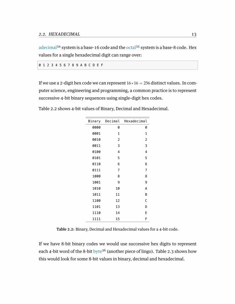
If we use a 2-digit hex code we can represent 16∗16 = 256 distinct values. In com-puter science, engineering and programming, a common practice is to representsuccessive 4-bit binary sequences using single-digit hex codes.
Table 2.2 shows 4-bit values of Binary, Decimal and Hexadecimal.
Binary Decimal Hexadecimal
0000 0 0
0001 1 1
0010 2 2
0011 3 3
0100 4 4
0101 5 5
0110 6 6
0111 7 7
1000 8 8
1001 9 9
1010 10 A
1011 11 B
1100 12 C
1101 13 D
1110 14 E
1111 15 F
Table 2.2: Binary, Decimal and Hexadecimal values for a 4-bit code.
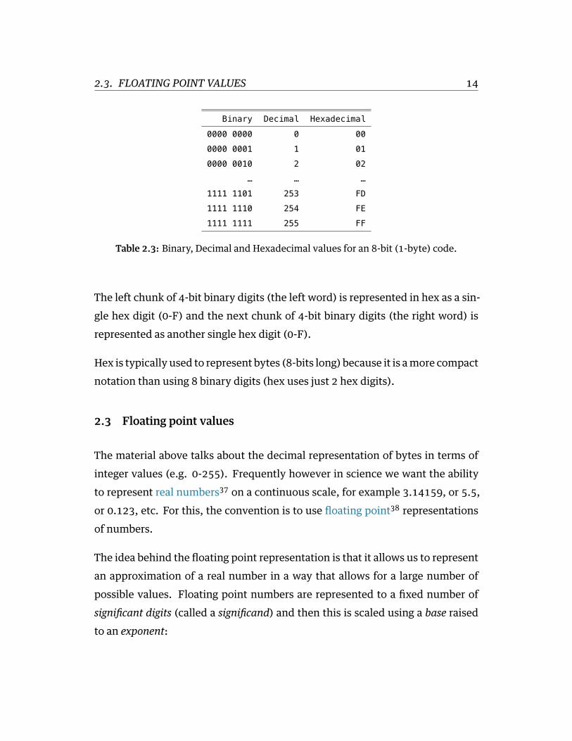
If we have 8-bit binary codes we would use successive hex digits to representeach 4-bit word of the 8-bit byte36 (another piece of lingo). Table 2.3 shows howthis would look for some 8-bit values in binary, decimal and hexadecimal.
2.3. FLOATING POINT VALUES 14
Binary Decimal Hexadecimal
0000 0000 0 00
0000 0001 1 01
0000 0010 2 02
… … …
1111 1101 253 FD
1111 1110 254 FE
1111 1111 255 FF
Table 2.3: Binary, Decimal and Hexadecimal values for an 8-bit (1-byte) code.
The left chunk of 4-bit binary digits (the left word) is represented in hex as a sin-gle hex digit (0-F) and the next chunk of 4-bit binary digits (the right word) isrepresented as another single hex digit (0-F).
Hex is typically used to represent bytes (8-bits long) because it is amore compactnotation than using 8 binary digits (hex uses just 2 hex digits).
2.3 Floating point values
The material above talks about the decimal representation of bytes in terms ofinteger values (e.g. 0-255). Frequently however in science we want the abilityto represent real numbers37 on a continuous scale, for example 3.14159, or 5.5,or 0.123, etc. For this, the convention is to use floating point38 representationsof numbers.
The idea behind the floating point representation is that it allows us to representan approximation of a real number in a way that allows for a large number ofpossible values. Floating point numbers are represented to a fixed number ofsignificant digits (called a significand) and then this is scaled using a base raisedto an exponent:

2.3. FLOATING POINT VALUES 15
s x be (2.1)
This is related to something you may have come across in high-school science,namely scientific notation39. In scientific notation, the base is 10 and so a realnumber like 123.4 is represented as 1.234 x 10².
In computers there are different conventions for different CPUs but there arestandards, like the IEEE 75440 floating-point standard. As an example, a so-called single-precision floating point format41 is represented in binary (using abase of 2) using 32 bits (4 bytes) and a /double precision/ floating point numberis represented using 64 bits (8 bytes). In C you can find out how many bytes areused for various types using the sizeof() function:
#include <stdio.h>
int main(int argc, char *argv[]) {
printf("a single precision float uses %ld bytes\n", sizeof(float));
printf("a double precision float uses %ld bytes\n", sizeof(double));
return 0;
}
On my macbook pro laptop this results in this output:
a single precision float uses 4 bytes
a double precision float uses 8 bytes
According to the IEEE754 standard, a singleprecision32-bit binaryfloatingpointrepresentation is composed of a 1-bit sign bit (signifying whether the number ispositive or negative), an 8-bit exponent and a 23-bit significand. See the variouswikipedia pages for full details.
There is a key phrase in the description of floating point values above, which is

2.3. FLOATING POINT VALUES 16
that floating point representation allows us to store an approximation of a realnumber. If we attempt to represent a number that has more significant digitsthan can be store in a 32-bit floating point value, then we have to approximatethat real number, typically by rounding off the digits that cannot fit in the 32 bits.This introduces rounding error42.
Now with 32 bits, or even 64-bits in the case of double precision floating pointvalues, rounding error is likely to be relatively small. However it’s not zero, anddepending on what your program is doing with these values, the rounding errorscan accumulate (for example if you’re simulating a dynamical system over thou-sands of time steps, and at each time step there is a small rounding error).
We don’t need a fancy simulation however to see the results of floating pointrounding error. Open up your favourite programming language (MATLAB,Python, R, C, etc) and type the following (adjust the syntax as needed for yourlanguage of choice):
(0.1 + 0.2) == 0.3
What do you get? In MATLAB I get:
>> (0.1 + 0.2) == 0.3
ans =
0
In MATLAB, 0 is synonymous with the logical value FALSE. What’s going on here?What’s happening is that these decimal numbers, 0.1, 0.2 and 0.3 are being rep-resented by the computer in a binary floating-point format, that is, using a base2 representation. The issue is that in base 2, the decimal number 0.1 cannot

2.3. FLOATING POINT VALUES 17
be represented precisely, no matter how many bits you use. Plug in the deci-mal number 0.1 into an online binary/decimal/hexadecimal converter (such ashere43) and you will see that the binary representation of 0.1 is an infinitely re-peating sequence:
0.000110011001100110011001100... (base 2)
This shouldn’t be an unfamiliar situation, if we remember that there are also realnumbers that cannot be represented precisely in decimal format, either, becausethey involve an infintely repeating sequence. For example the real number 1
3when represented in decimal44 is:
0.3333333333... (base 10)
If we try to represent 13 using n decimal digits then we have to chop off the digits
to the right that we cannot include, thereby rounding the number. We lose someamount of precision that depends onhowmany significant digitswe retain in ourrepresentation.
So the same is true in binary. There are some real numbers that cannot be repre-sented precisely in binary floating-point format.
See here45 for some examples of significant adverse events (i.e. disasters) causeby numerical errors.
Rounding canbeused toyour advantage, if you’re in thebusinessof stealing frompeople (see salami slicing46). In the awesomely kitchy 1980s movie SupermanIII47, Richard Pryor’s character plays a “bumbling computer genius” who embez-zles a ton of money by stealing a large number of fractions of cents (which in themovie are said to be lost anyway due to rounding) from his company’s payroll(YouTube clip here48).

2.4. ASCII 18
There is a comprehensive theoretical summary of these issues here: What EveryComputer Scientist Should Know About Floating-Point Arithmetic49.
Also see these webpages from the MathWorks online documentation about howMATLAB represents floating-point numbers:
Floating-Point Numbers50
and this section on avoiding common problems with Floating-Point Arithmetic:
Avoiding Common Problems with Floating-Point Arithmetic51
2.4 ASCII
ASCII stands for American Standard Code for Information Interchange. ASCIIcodes delineate how text is represented in digital format for computers (as wellas other communications equipment).
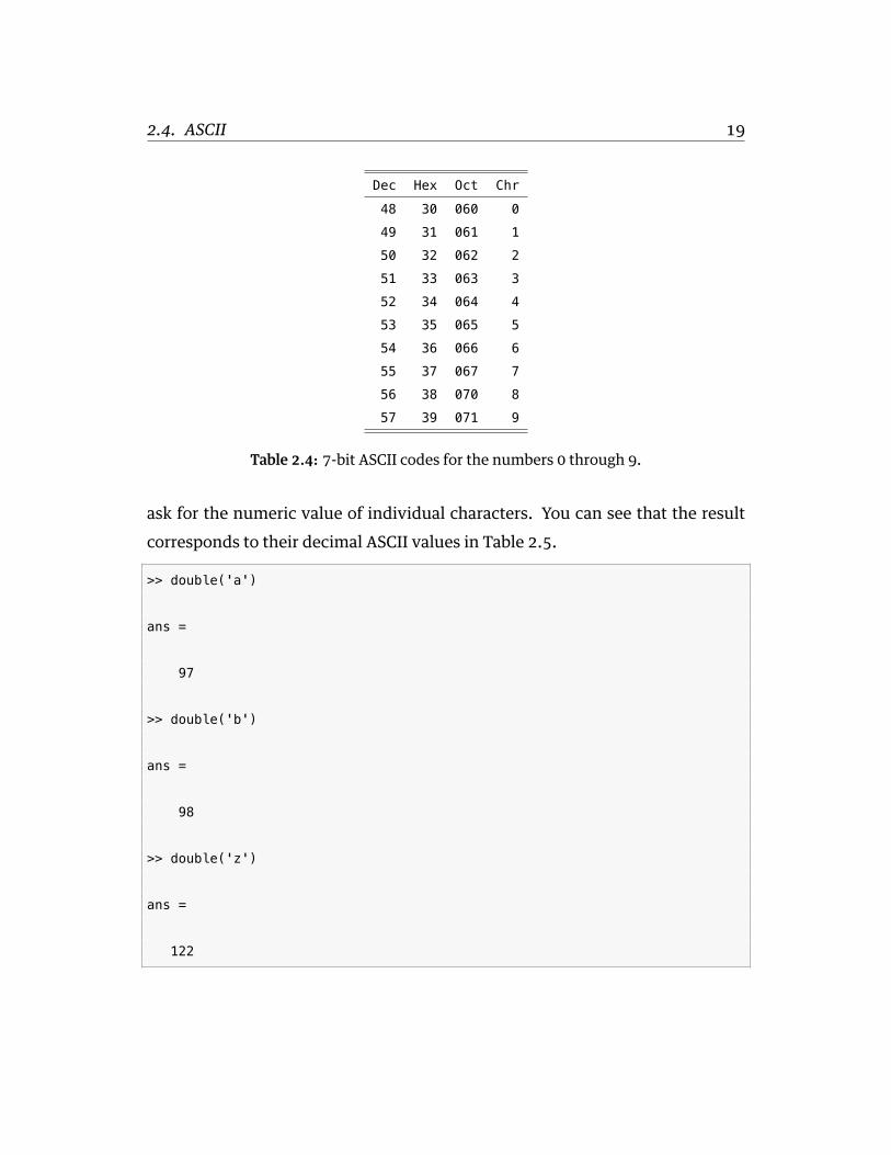
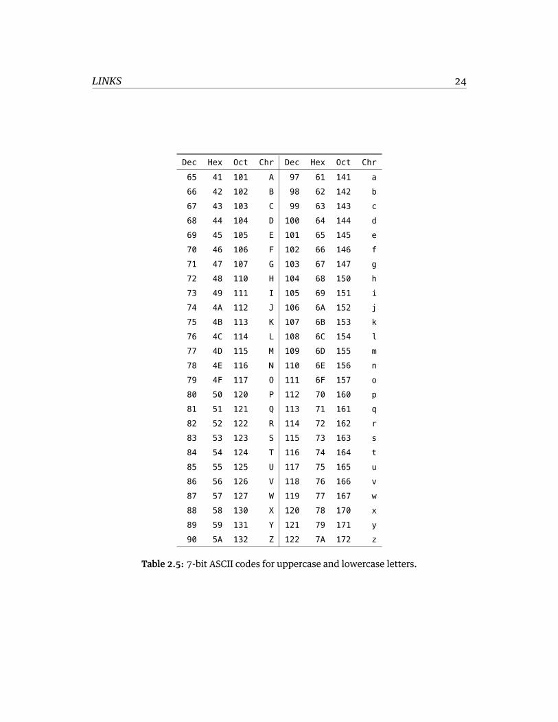
ASCII uses a 7-bit binary code to represent 128 specific characters of text. Thefirst 32 codes (decimal 0 through 31) are non-printable codes like TAB, BEL (playa bell sound), CR (carriage return), etc. Decimal codes 32 through 47 are moretypical text symbols like # and &. Decimal codes 48 through 57 are the numbers0 through 9. Decimal codes 65 through 90 are capital letters A through Z, andcodes 97 through 122 are lowercase letters a through z. Table 2.4 shows codes indecimal, hexadecimal and octal (base-8) for the numbers 0 through 9. Table 2.5shows codes for uppercase and lowercase letters.
For a full description of the 7-bit ascii codes in their entirety, including the ex-tended ASCII codes (where you will find things like ö and é), see this webpage:
http://www.asciitable.com52 (ASCII Table and Extended ASCII Codes).
In MATLAB, all individual text characters (variable type char) are represented,under the hood, as decimal ASCII values. Have a look at this code, in which we
2.4. ASCII 19
Dec Hex Oct Chr
48 30 060 0
49 31 061 1
50 32 062 2
51 33 063 3
52 34 064 4
53 35 065 5
54 36 066 6
55 37 067 7
56 38 070 8
57 39 071 9
Table 2.4: 7-bit ASCII codes for the numbers 0 through 9.
ask for the numeric value of individual characters. You can see that the resultcorresponds to their decimal ASCII values in Table 2.5.
>> double('a')
ans =
97
>> double('b')
ans =
98
>> double('z')
ans =
122

2.4. ASCII 20
You can get the character value of an ASCII code in MATLAB using the char()
function:
>> char(65)
ans =
A
You can use your knowledge of ASCII codes to do tricky things in MATLAB, likeconvert to and from uppercase and lowercase, given your knowledge that thedifference (in decimal) between ASCII A and ASCII a is 32 (see Table 2.5).
>> char('A' + 32)
ans =
a
>> char('a' - 32)
ans =
A

2.4. ASCII 21
Exercises
E 2.1 Convert the following decimal integer values into hexadecimal (resist theurge to use an online decimal–to–hex tool, try to do it using your brain):
1. 642062. 478063. 40134. 642225. 47802
E 2.2 Convert the following decimal integer values into binary (little-endian for-mat):
1. 22. 203. 2004. 175. 170
E 2.3 Convert the following (little-endian) binary values into hexadecimal:
1. 00012. 10003. 10014. 1000 00015. 1011 1010 1011 1010

LINKS 22
Links
29http://en.wikipedia.org/wiki/Binary_code
30http://en.wikipedia.org/wiki/Bit
31http://en.wikipedia.org/wiki/Endianness
32http://en.wikipedia.org/wiki/Word_(computer_architecture)
33http://www.asciitable.com
34http://en.wikipedia.org/wiki/Hexadecimal
35http://en.wikipedia.org/wiki/Octal
36http://en.wikipedia.org/wiki/Byte
37http://en.wikipedia.org/wiki/Real_number
38http://en.wikipedia.org/wiki/Floating_point
39http://en.wikipedia.org/wiki/Scientific_notation
40http://en.wikipedia.org/wiki/IEEE_floating_point
41http://en.wikipedia.org/wiki/Binary32
42http://en.wikipedia.org/wiki/Round-off_error
43http://www.wolframalpha.com/input/?i=0.1+to+binary
44http://www.wolframalpha.com/input/?i=1%2F3+in+decimal
45http://ta.twi.tudelft.nl/users/vuik/wi211/disasters.html
46http://en.wikipedia.org/wiki/Salami_slicing
47http://en.wikipedia.org/wiki/Superman_III
48http://www.youtube.com/watch?v=iLw9OBV7HYA
49http://docs.oracle.com/cd/E19957-01/806-3568/ncg_goldberg.html
50http://www.mathworks.com/help/matlab/matlab_prog/floating-point-numbers.html
51http://www.mathworks.com/help/matlab/matlab_prog/floating-point-numbers.html#
bqxyrhp
LINKS 24
Dec Hex Oct Chr Dec Hex Oct Chr
65 41 101 A 97 61 141 a
66 42 102 B 98 62 142 b
67 43 103 C 99 63 143 c
68 44 104 D 100 64 144 d
69 45 105 E 101 65 145 e
70 46 106 F 102 66 146 f
71 47 107 G 103 67 147 g
72 48 110 H 104 68 150 h
73 49 111 I 105 69 151 i
74 4A 112 J 106 6A 152 j
75 4B 113 K 107 6B 153 k
76 4C 114 L 108 6C 154 l
77 4D 115 M 109 6D 155 m
78 4E 116 N 110 6E 156 n
79 4F 117 O 111 6F 157 o
80 50 120 P 112 70 160 p
81 51 121 Q 113 71 161 q
82 52 122 R 114 72 162 r
83 53 123 S 115 73 163 s
84 54 124 T 116 74 164 t
85 55 125 U 117 75 165 u
86 56 126 V 118 76 166 v
87 57 127 W 119 77 167 w
88 58 130 X 120 78 170 x
89 59 131 Y 121 79 171 y
90 5A 132 Z 122 7A 172 z
Table 2.5: 7-bit ASCII codes for uppercase and lowercase letters.
3 Basic data types, operators & expressions
3.1 Expressions
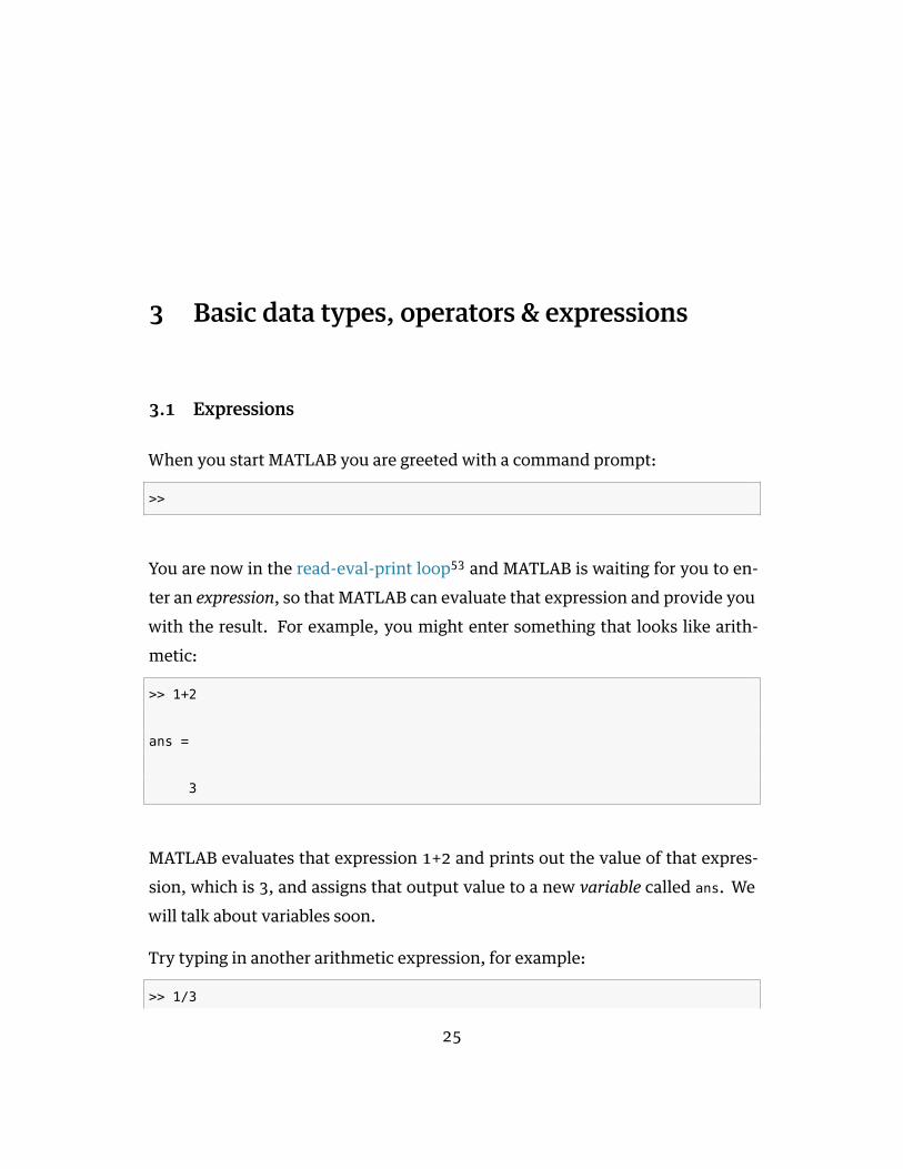
When you start MATLAB you are greeted with a command prompt:
>>
You are now in the read-eval-print loop53 and MATLAB is waiting for you to en-ter an expression, so that MATLAB can evaluate that expression and provide youwith the result. For example, you might enter something that looks like arith-metic:
>> 1+2
ans =
3
MATLAB evaluates that expression 1+2 and prints out the value of that expres-sion, which is 3, and assigns that output value to a new variable called ans. Wewill talk about variables soon.
Try typing in another arithmetic expression, for example:
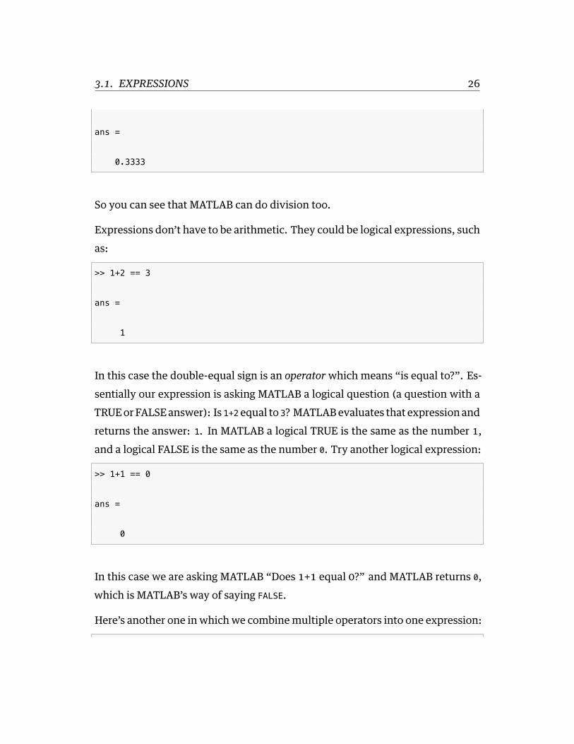
>> 1/3
25
3.1. EXPRESSIONS 26
ans =
0.3333
So you can see that MATLAB can do division too.
Expressions don’t have to be arithmetic. They could be logical expressions, suchas:
>> 1+2 == 3
ans =
1
In this case the double-equal sign is an operator which means “is equal to?”. Es-sentially our expression is asking MATLAB a logical question (a question with aTRUEorFALSEanswer): Is 1+2 equal to 3? MATLABevaluates that expressionandreturns the answer: 1. In MATLAB a logical TRUE is the same as the number 1,and a logical FALSE is the same as the number 0. Try another logical expression:
>> 1+1 == 0
ans =
0
In this case we are asking MATLAB “Does 1+1 equal 0?” and MATLAB returns 0,which is MATLAB’s way of saying FALSE.
Here’s another one in which we combine multiple operators into one expression:
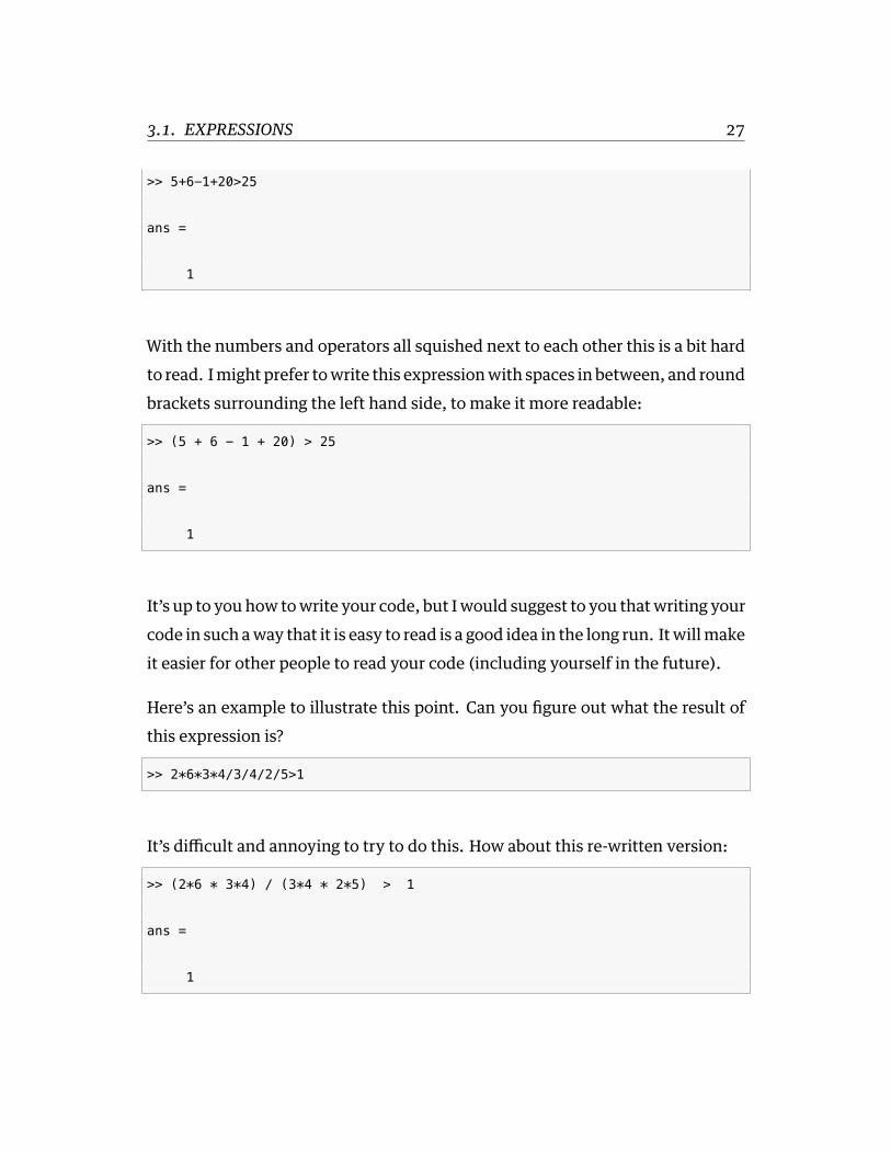
3.1. EXPRESSIONS 27
>> 5+6-1+20>25
ans =
1
With the numbers and operators all squished next to each other this is a bit hardto read. Imight prefer towrite this expressionwith spaces in between, and roundbrackets surrounding the left hand side, to make it more readable:
>> (5 + 6 - 1 + 20) > 25
ans =
1
It’s up to youhow towrite your code, but Iwould suggest to you thatwriting yourcode in such away that it is easy to read is a good idea in the long run. Itwillmakeit easier for other people to read your code (including yourself in the future).
Here’s an example to illustrate this point. Can you figure out what the result ofthis expression is?
>> 2*6*3*4/3/4/2/5>1
It’s difficult and annoying to try to do this. How about this re-written version:
>> (2*6 * 3*4) / (3*4 * 2*5) > 1
ans =
1

3.2. OPERATORS 28
They are both valid code, they both evaluate to the same result, but one version(the second version) is much more readable (in my opinion).
Here’s a puzzling result:
>> 0.1 + 0.2 == 0.3
ans =
0
This is a rather surprising result, isn’t it. I’ll leave it as an exercise for you toresearch why this happens, and what a potential solution to this kind of unex-pected result might be. Hint: look at the course notes on digital representationof data54.
Let’s move on and talk about operators.
3.2 Operators
In the example code snippets above we saw a number of operators already. Wesaw the + and / mathematical operators, and we saw the logical operator ==.There are in fact a wide variety of operators in MATLAB. The MathWorks (thecompany that makes MATLAB) has a web page that lists them all:
Operators and Elementary Operations55
There are a variety of arithmetics operators, relational and logical operators, andothers that you can read about as well.
One concept that is important to talk about is operator precedence. This refersto the order in which MATLAB evaluates expressions and operators when thereare multiple operations in a single expression. Take the following expression for
3.2. OPERATORS 29
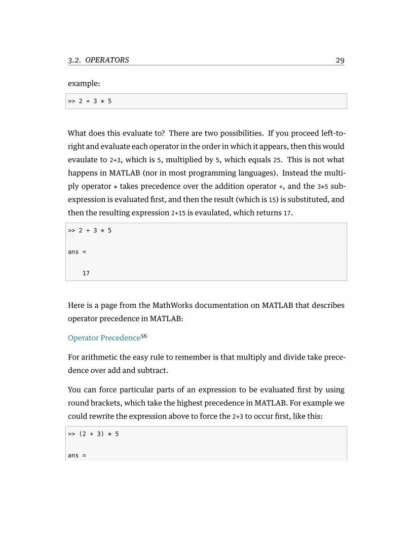
example:
>> 2 + 3 * 5
What does this evaluate to? There are two possibilities. If you proceed left-to-right and evaluate each operator in the order inwhich it appears, then thiswouldevaulate to 2+3, which is 5, multiplied by 5, which equals 25. This is not whathappens in MATLAB (nor in most programming languages). Instead the multi-ply operator * takes precedence over the addition operator +, and the 3*5 sub-expression is evaluated first, and then the result (which is 15) is substituted, andthen the resulting expression 2+15 is evaulated, which returns 17.
>> 2 + 3 * 5
ans =
17
Here is a page from the MathWorks documentation on MATLAB that describesoperator precedence in MATLAB:
Operator Precedence56
For arithmetic the easy rule to remember is that multiply and divide take prece-dence over add and subtract.
You can force particular parts of an expression to be evaluated first by usinground brackets, which take the highest precedence in MATLAB. For example wecould rewrite the expression above to force the 2+3 to occur first, like this:
>> (2 + 3) * 5
ans =

3.3. VARIABLES 30
25
3.3 Variables
In the above examples we have been typing in numbers, along with arithmeticand logical or relational operators, andMATLABevaluates those expressions andreturns the result. In factwhenyoudon’t provide anyoutput variable to store theresults of your expression, MATLAB automatically stores the result in a variablecalled ans (short for answer). So for example:
>> 1 + 2
ans =
3
MATLABhas stored theanswer in avariable called ans. Youcan thinkof avariableas a human-readable nameof somedata that is stored inMATLAB’smemory. Youcan refer to data by it’s variable name. Under the hood, MATLAB keeps trackof how these variable names correspond to the location (and type) of the datastored in memory.
This memory we are referring to is RAM or Random-access memory57. This is aformof data storage in your computerwhich is to be considered temporary. OnceMATLAB quits, or your computer is turned off, the data that was stored in RAMis gone. To permanently store data on your computer you need to store it on amore permanent form of memory, such as the hard drive in your computer, or anexternal drive such as a memory stick.
By naming your data using a variable name, you can easily view and manipulate

3.3. VARIABLES 31
those data. Here’s an example where we store the result of a calculation in a vari-able that we will name fred:
>> fred = 1 + 2
fred =
3
We type our expression 1+2 and on the left hand side we type our variable namefred, and set it to be equal to (using the equal sign =) the expression. MATLABevaluates this whole expression and in its return statement we can see that nowfred is equal to 3.
Here’s another one:
>> bob = 4 * 5
bob =
20
Now we have defined a second variable called bob which we have set to be equalto the result of the expression 4*5. We can see inMATLAB’s return statement thatnow bob is equal to 20.
We can use variable names within expressions and MATLAB will substitute thevalue of those variables within the expression:
>> joe = bob + fred
joe =
23

3.3. VARIABLES 32
We have defined a new variable called joe and assigned it to be equal to the valueof bob (which is 20) added to the value of fred (which is 3). MATLAB returns thatnow joe is equal to 23.
What happens if we do this?
>> mike = joe + bob + fred + danny
Undefined function or variable 'danny'.
MATLAB returns an error: Undefined function or variable 'danny'. The prob-lem here is that we have never defined a variable called danny and so when MAT-LAB attempts to evaluate danny, it can’t find anything. When it evaluates joe andbob and fredMATLAB knows the data that those variable names refers to, but wehave not named any data using a variable called danny and so MATLAB has noidea what we are referring to.
In fact this is exactly the right way to think about this error: when we type danny,MATLAB does not know what we are referring to.
At any time we can get a list of which variables are defined in MATLAB by usinga command called who:
Your variables are:
bob fred joe
We can see we have three variables defined. You can use a command called whos
to get a more detailed list:
>> whos
Name Size Bytes Class Attributes
3.3. VARIABLES 33
bob 1x1 8 double
fred 1x1 8 double
joe 1x1 8 double
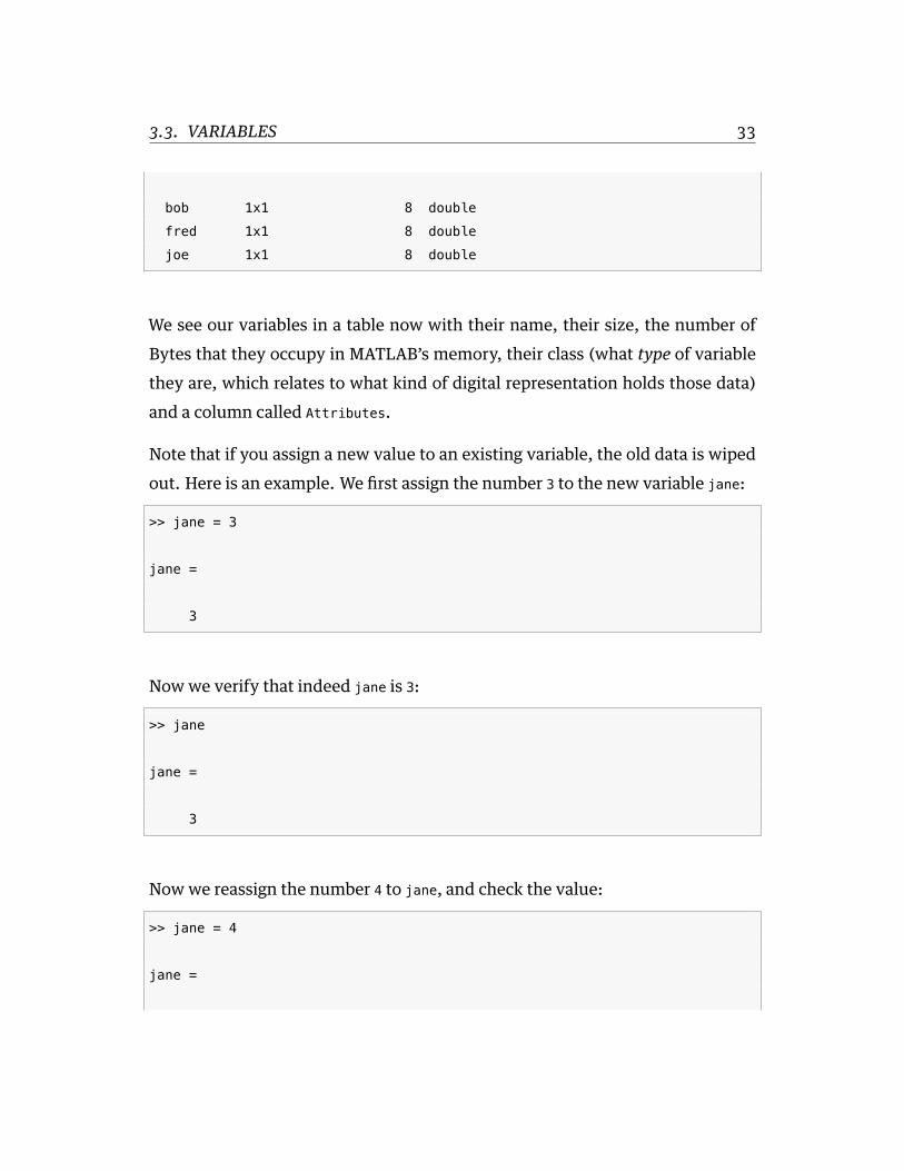
We see our variables in a table now with their name, their size, the number ofBytes that they occupy in MATLAB’s memory, their class (what type of variablethey are, which relates to what kind of digital representation holds those data)and a column called Attributes.
Note that if you assign a new value to an existing variable, the old data is wipedout. Here is an example. We first assign the number 3 to the new variable jane:
>> jane = 3
jane =
3
Now we verify that indeed jane is 3:
>> jane
jane =
3
Now we reassign the number 4 to jane, and check the value:
>> jane = 4
jane =

3.3. VARIABLES 34
4
>> jane
jane =
4
Indeed, jane is now 4 and there is no trace of 3.
There are some rules governing how you can name your variables. Variablenames cannot start with a number or a symbol, only with a letter. There canbe no spaces or symbols in variable names. Capitalization matters, so joe is dif-ferent than Joe.
The other thing to talk about in this context is thatMATLABhas some commandsand functions that are already defined by MATLAB, and so you should avoid us-ing those as your own variable names. So for example MATLAB has a built-infunction called sort() that will sort a vector of values:
>> sort([4 3 2 6 5 7 9 8 1])
ans =
1 2 3 4 5 6 7 8 9
When you type sort MATLAB executes its built-in sorting algorithm. Nothingstops you however from defining your own variable with the same name:
>> sort = 23
sort =

3.3. VARIABLES 35
23
Now when you try typing the sorting expression in again you get this:
>> sort([4 3 2 6 5 7 9 8 1])
Index exceeds matrix dimensions.
MATLABthrowsanerror. NowwhenMATLABsees sort it thinksyouare referringto your variable called sort which equals 23. Actually it equals a 1x1 matrix (asingle value) containing 23.
Why do we get this particular error message? The round brackets when put nextto a variable cause MATLAB to try to index into a vector or matrix, and since ourvariable sort has only a single value, when MATLAB tries to retrieve the 4th, then3rd, then 2nd, values, etc, it throws an error. We haven’t talked about vectorsor matrices or indexing yet, so don’t worry about that. The point here is thatwe have essentially wiped out the reference to the sorting algorithm originallyreferred to by sort by defining our own variable called sort. Oops!
We can remedy this situation by clearing the variable sort using the built-in com-mand clear:
>> clear sort
Now we have erased our variable called sort and when we type sort again, MAT-LAB will no longer refer to our variable containing 23 (since we just cleared itfrom memory) and MATLAB will go back to referring to its own built-in functioncalled sort():
>> sort([4 3 2 6 5 7 9 8 1])
ans =

3.4. BASIC DATA TYPES 36
1 2 3 4 5 6 7 8 9
Now it’s time to talk about variable types.
3.4 Basic Data Types
So farwehave beendealingwith data in the formof single numbers. Thenumber1 for example, or the number 0.5. There are in fact a number of different numerictypes of data that MATLAB can store in variables. Here is a webpage from theMathWorks that describes the full constellation of data types used in MATLAB:
Data Types58
Numeric data can be stored in a number of different Numeric Types59. Thedefault type of numeric data in MATLAB is double, which stands for double-precision floating-point format60. The floating-point part of this means essen-tially that this data type can store a real number61, i.e. numbers along a contin-uous line such as 1.0 or 1.33 or 3.14159. The double-precision part of this refersto how many bytes are used by MATLAB to represent that number. More bytesmeans more precision. You can read about this in more detail in Chapter 2, Digi-tal representation of data.
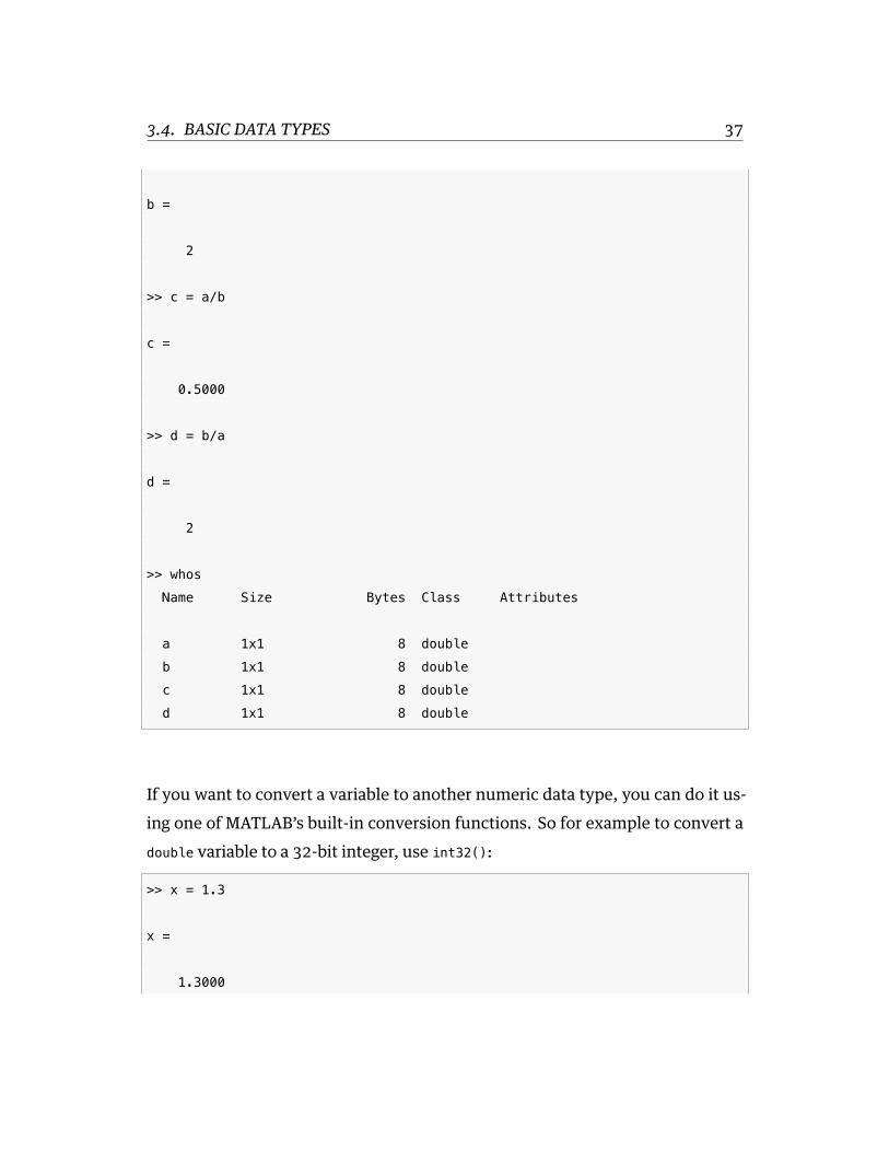
When you just type in numbers, or have MATLAB compute the result of an arith-metic expression, you will typically be using, by default, the double data type:
>> a = 1
a =
1
>> b = 2
3.4. BASIC DATA TYPES 37
b =
2
>> c = a/b
c =
0.5000
>> d = b/a
d =
2
>> whos
Name Size Bytes Class Attributes
a 1x1 8 double
b 1x1 8 double
c 1x1 8 double
d 1x1 8 double
If you want to convert a variable to another numeric data type, you can do it us-ing one of MATLAB’s built-in conversion functions. So for example to convert adouble variable to a 32-bit integer, use int32():
>> x = 1.3
x =
1.3000

3.4. BASIC DATA TYPES 38
>> y = int32(x)
y =
1
>> whos
Name Size Bytes Class Attributes
x 1x1 8 double
y 1x1 4 int32
You can see that when the double x (which equals 1.3) is converted into an int32
it is rounded down to 1.
MATLAB also has data types to deal with individual characters (letters like 'a'
and 'b') and stringsof characters (like 'joe'), anda selectionof built-in functionsto manipulate strings:
Characters and Strings62
For example:
>> x = 'a'
x =
a
>> y = 'b'
y =
b

3.4. BASIC DATA TYPES 39
>> z = 'fred'
z =
fred
>> whos
Name Size Bytes Class Attributes
x 1x1 2 char
y 1x1 2 char
z 1x4 8 char
Abovewehavedefined three variables all of type char (which stands for characterstring). The first two, named x and y both contain a single character ('a' and 'b',respectively) and the third, z, contains a string of four characters ('fred'). Youcan see that x and y occupy 2 bytes of memory and z uses 8 bytes. Two bytes arerequired to store a single character in MATLAB.
You can dive deeper here in the documentation for the char function63, whichdescribes how characters are represented. The first 7 bits (values 0 to 127) code7-bit ASCII characters. The next 9 bits code values 128 to 65535 and representcharacters that depend on your locale (i.e. other languages besides plain englishASCII).
Youcanquickly see the integer codes fordifferent characters inMATLABbydoingthe following:
>> int8('a')
ans =

3.4. BASIC DATA TYPES 40
97
>> int8('b')
ans =
98
>> int8('z')
ans =
122
In fact you can get the integer codes for all 26 lower case letters in one go, likethis:
>> int8('a':'z')
ans =
Columns 1 through 15
97 98 99 100 101 102 103 104 105 106 107 108 109 110 111
Columns 16 through 26
112 113 114 115 116 117 118 119 120 121 122
You can display a string to the screen using the disp command:
>> disp('hello, world, my name is fred')
hello, world, my name is fred

3.4. BASIC DATA TYPES 41
You can concatenate multiple strings using the square brackets [ and ] to con-struct a new string:
>> a = 'fred';
>> b = 'joe';
>> c = 'jane';
>> s = ' ';
>> z = [a,s,b,s,c];
>> disp(z)
fred joe jane
I’ve introduced some new syntax here, the use of the semicolon ; after an ex-pression. This prevents MATLAB from echoing the value of the expression tothe screen. The expression is still evaluated but MATLAB doesn’t echo the resultback to us on the screen. Use this when you want to suppress the output of ex-pressions. If you don’t need to see the result of an expression on the screen thenthis makes for a cleaner MATLAB session.
You can get attributes of a string such as its length:
>> disp(['z is ', num2str(l), ' characters long'])
z is 13 characters long
I’ve also introducted the built-in function num2str()whichwill convert a numerictype into a character string.
Another way to generate a character string out of many parts is to use thesprintf() function. This mimics the printf() function64 that is famililar to C pro-grammers:
>> m = sprintf('z is %d characters long, & pi is approx. %.5f', l, pi);
>> disp(m)
z is 13 characters long, and pi is approximately 3.14159

3.4. BASIC DATA TYPES 42
The %d notation tells the sprintf function that an integer numeric type will be pro-vided here. The %.5f notation says that a floating-point value will be provided,and please show it using 5 decimal places. At the end of the string is where yousupply the needed values, in the order in which they appear in the string. Notethat pi is a built-in value in MATLAB.
In MATLAB you can use the class() function to get the type of a variable. Forexample:
>> a = 3.14159
a =
3.1416
>> class(a)
ans =
double
You can use the isa() function to ask whether a variable is a certain type. Forexample:
>> isa(a,'char')
ans =
0
>> isa(a,'double')
ans =

3.5. SPECIAL VALUES 43
1
Remember in MATLAB 0 is “FALSE” or “NO” and 1 is “TRUE” or “YES”.
So far we have seen numeric types and character string types. These are basicdata types. MATLABalso allows for complexdata types such as vectors,matrices,structures and cell arrays. These you can think of as container types, in otherwords data types that can store not just one value but many values.
Actually, the character string is already a sort of container type, in that it storesmany single characters all strung together. You can think of a character string asa vector of single characters.
In the next section in the notes we will talk about some of these complex datatypes and how to use them.
3.5 Special values
The MathWorks online documentation has a page on various special values built-in to MATLAB:
Special Values65
There is a special numeric value in MATLAB called NaN (not a number). It is oftenused to denote missing data.
There is also a special value called Inf which stands for infinity. Try typing theexpression 1/0 and you will get Inf.
There are other mathematical special values such as pi:
>> pi
ans =

3.5. SPECIAL VALUES 44
3.1416
>> help pi
PI 3.1415926535897....
PI = 4*atan(1) = imag(log(-1)) = 3.1415926535897....
Reference page in Help browser
doc pi
and imaginary numbers i and j:
>> help i
I Imaginary unit.
As the basic imaginary unit SQRT(-1), i and j are used to enter
complex numbers. For example, the expressions 3+2i, 3+2*i, 3+2j,
3+2*j and 3+2*sqrt(-1) all have the same value.
Since both i and j are functions, they can be overridden and used
as a variable. This permits you to use i or j as an index in FOR
loops, etc.
See also J.
Reference page in Help browser
doc i
>> help j
J Imaginary unit.
As the basic imaginary unit SQRT(-1), i and j are used to enter
complex numbers. For example, the expressions 3+2i, 3+2*i, 3+2j,
3+2*j and 3+2*sqrt(-1) all have the same value.
Since both i and j are functions, they can be overridden and used
as a variable. This permits you to use i or j as an index in FOR
loops, subscripts, etc.

3.5. SPECIAL VALUES 45
See also I.
Reference page in Help browser
doc j
Also of note is the special function eps():
>> help eps
EPS Spacing of floating point numbers.
D = EPS(X), is the positive distance from ABS(X) to the next larger in
magnitude floating point number of the same precision as X.
X may be either double precision or single precision.
For all X, EPS(X) is equal to EPS(ABS(X)).
EPS, with no arguments, is the distance from 1.0 to the next larger
double
precision number, that is EPS with no arguments returns 2^(-52).
...
If we type eps(1.0) we get:
>> eps(1.0)
ans =
2.2204e-16
which is a pretty small number: 0.00000000000000022204. This is the distance be-tween the floating-point representation of 1.0 and the next largest number thatthe double floating-point representation can represent. You can think of it as theprecision of the double floating-point representation of numbers, near the num-
3.6. GETTING HELP 46
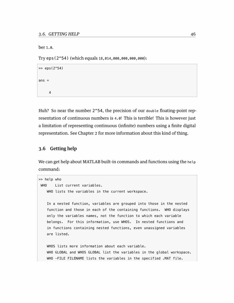
ber 1.0.
Try eps(2^54) (which equals 18,014,000,000,000,000):
>> eps(2^54)
ans =
4
Huh? So near the number 2^54, the precision of our double floating-point rep-resentation of continuous numbers is 4.0! This is terrible! This is however justa limitation of representing continuous (infinite) numbers using a finite digitalrepresentation. See Chapter 2 for more information about this kind of thing.
3.6 Getting help
We can get help about MATLAB built-in commands and functions using the help
command:
>> help who
WHO List current variables.
WHO lists the variables in the current workspace.
In a nested function, variables are grouped into those in the nested
function and those in each of the containing functions. WHO displays
only the variables names, not the function to which each variable
belongs. For this information, use WHOS. In nested functions and
in functions containing nested functions, even unassigned variables
are listed.
WHOS lists more information about each variable.
WHO GLOBAL and WHOS GLOBAL list the variables in the global workspace.
WHO -FILE FILENAME lists the variables in the specified .MAT file.

3.6. GETTING HELP 47
WHO ... VAR1 VAR2 restricts the display to the variables specified. The
wildcard character '*' can be used to display variables that match a
pattern. For instance, WHO A* finds all variables in the current
workspace that start with A.
WHO -REGEXP PAT1 PAT2 can be used to display all variables matching the
specified patterns using regular expressions. For more information on
using regular expressions, type "doc regexp" at the command prompt.
Use the functional form of WHO, such as WHO('-file',FILE,V1,V2),
when the filename or variable names are stored in strings.
S = WHO(...) returns a cell array containing the names of the variables
in the workspace or file. You must use the functional form of WHO when
there is an output argument.
Examples for pattern matching:
who a* % Show variable names starting with "a"
who -regexp ^b\d{3}$ % Show variable names starting with "b"
% and followed by 3 digits
who -file fname -regexp \d % Show variable names containing any
% digits that exist in MAT-file fname
See also WHOS, CLEAR, CLEARVARS, SAVE, LOAD.
Other functions named who:
Simulink.who
Reference page in Help browser
doc who
We can also get a GUI interface to help using the doc command.
There is also away of searching the help documentation files for keywords, using

3.7. SCRIPT M-FILES 48
the lookfor command. The lookfor command will return the names of all func-tions or commands for which the associated help documentation contains thegiven keyword. So for example let’s say we need to find the invkine() functionbut we’ve forgotten what it’s called, we just remember it’s something to do witha robot. We can search using: lookfor robot
>> lookfor robot
invkine - Inverse kinematics of a robot arm.
invkine_codepad - Modeling Inverse Kinematics in a Robotic
Arm
idnlgreydemo13 - Modeling an Industrial Robot Arm
idnlgreydemo8 - Industrial Three-Degrees-of-Freedom Robot:
C MEX-File Modeling of MIMO System Using Vector/Matrix Parameters
robot_m - A simplified Manutec r3 robot with three
arms.
robotarm_m - A physically parameterized robot arm.
refmodel_dataset - ROBOTARM_DATASET Reference model dataset
robotarm_dataset - Robot arm dataset
mech_robot_data - Data defining the manutec robot.
RobotArmExample - Multi-Loop PID Control of a Robot Arm
3.7 Script M-files
Instead of typing in commands into theMATLAB command-line, you can insteadsave them in a file, called a MATLAB script, and then type the name of the scripton the command line to execute all codewithin that script. Scripts typically havea .m filename suffix.
So for example you might have a file called random8.m that contains the followingcode:
% script M-file example random8.m
%

3.8. MATLAB PATH 49
rlist = round(rand(1,8)*10);
disp(rlist);
disp(['mean = ',num2str(mean(rlist))]);
disp(['median = ',num2str(median(rlist))]);
disp(['standard deviation = ',num2str(std(rlist))]);
The script generates a list of 8 random numbers chosen from a uniform distribu-tion between 0 and 10, and then displays the mean, median and standard devia-tion of those values.
If the script file called random8.m is in your MATLAB path, then typing random8.m
on the MATLAB command line will execute the script:
>> random8
8 9 1 9 6 1 3 5
mean = 5.25
median = 5.5
standard deviation = 3.3274
3.8 MATLAB path
When you first start MATLAB, you will be faced with the command line prompt,andMATLABwill be startedup looking at a particular location in your file system.This location is known as the current working directory. If you are using the MAT-LAB GUI (graphical user interface) you will see your current working directorydisplayed in a toolbar just above the command line. On my computer it shows as/Users/plg/Desktop. On your computer it will be something different.
The other way to query MATLAB about the current working directory is to typepwd into the command line:

3.8. MATLAB PATH 50
>> pwd
ans =
/Users/plg/Desktop
When you type something into the command line, like random8, MATLAB will gothrough a number of steps to find out what you mean:
• is random8 defined as a variable in memory?• is random8defined as a function or script file or data file inMATLAB’s current
working directory?• is random8 defined as a function or script file or data file somewhere else in
MATLAB’s path?
TheMATLABpath is a list of directories onyour computer’s harddiskwhereMAT-LAB knows to look for scripts and functions. You can see what’s defined in yourMATLAB path by typing path at the MATLAB command line:
>> path
MATLABPATH
/Users/plg/Documents/MATLAB
/Applications/MATLAB_R2015a.app/toolbox/matlab/addons
/Applications/MATLAB_R2015a.app/toolbox/matlab/addons/cef
/Applications/MATLAB_R2015a.app/toolbox/matlab/addons/
fallbackmanager
/Applications/MATLAB_R2015a.app/toolbox/matlab/demos
/Applications/MATLAB_R2015a.app/toolbox/matlab/graph2d
/Applications/MATLAB_R2015a.app/toolbox/matlab/graph3d
/Applications/MATLAB_R2015a.app/toolbox/matlab/graphics
...
...

3.8. MATLAB PATH 51
On my computer I get a list of more than 600 directories—almost all of them sub-directories of the MATLAB main application directory. This is where all of MAT-LAB’s built-in functions and scripts are located, and where the various MATLABtoolbox code is located.
The other way to see (and alter) your MATLAB path is by using the MATLAB GUI.Type pathtool on the MATLAB command line and you get a nice GUI interfacewhere you can scroll through all of the directories that are in your MATLAB path,you can delete some, add some, and change the order.
On the issue of the order: remember that MATLAB goes through its path in theorder in which the directories appear in the path list. So if you have a functioncalled random8() defined in multiple places in your path, when you type random8
on the MATLAB command line, MATLAB will use the first one it finds in the path.
My personal approach to the MATLAB path is to basically never mess with it. In-stead of adding data directories and script directories associatedwithmyvariousprojects to the MATLAB path, instead I just start MATLAB from the appropriatelocation when I am working on different projects.
To change the current working directory you can either click on the toolbar inthe MATLAB GUI, or use the cd command on the MATLAB command line, forexample:
>> cd /Users/plg/Documents/Research/projects/Heather_fMRI/
>> pwd
ans =
/Users/plg/Documents/Research/projects/Heather_fMRI

3.8. MATLAB PATH 52
Exercises
E 3.1 Write a program to convert temperature values from Celsius to Fahrenheitaccording to the equation:
F =95C+ 32 (3.1)
The program should as the user to input the temperature in Celsius, andthen print out a sentence giving the temperature in Fahrenheit, like this:
enter the temperature in Celsius: 22
22.0 degrees Celsius is 71.6 degrees Fahrenheit
E 3.2 Given parabolic flight, the height of a ball y is given by the equation:
y = x tan(θ)−[ 12v20
] [ gx2cos(θ)2
]+ y0 (3.2)
where x is a horizontal coordinate (metres), g is the acceleration of gravity(metres per second per second), v0 is the size of the initial velocity vector(metres per second) at an angle θ (radians) with the x-axis, and (0, y0) is theinitial position of the ball (metres).
Write a program to compute the vertical height of a ball. The programshould ask the user to input values for g, v0, θ, x, and y0, and print out asentence giving the vertical height of the ball.
Test your program with this example:
enter a value for g: 9.8
enter a value for v0: 6.789
enter a value for theta: 0.123
enter a value for x: 4.5
enter a value for y0: 5.4

3.8. MATLAB PATH 53
The vertical height of the ball is: 3.77057803072
E 3.3 As an egg cooks, the proteins first denature and then coagulate. When thetemperature exceeds a critical point, reactions begin and proceed faster asthe temperature increases. In the egg white the proteins start to coagulatefor temperatures above63C,while in theyolk theproteins start to coagulatefor temperatures above 70 C. For a soft-boiled egg, the white needs to havebeen heated long enough to coagulate at a temperature above 63 C, but theyolk should not be heated above 70 C. For a hard-boiled egg, the centre ofthe yolk should be allowed to reach 70 C.
The following equation gives the time t it takes (in seconds) for the centreof the yolk to reach the temperature Ty (Celsius):
t = M2/3cρ1/3Kπ2(4π/3)2/3 ln
[0.76To − Tw
Ty − Tw
](3.3)
whereM, ρ, c and K are properties of the egg: M is mass, ρ is the density, c isthe specific heat capacity, and K is the thermal conductivity. Relevant val-ues areM = 47 g for a small egg andM = 67 g for a large egg, ρ = 1.038 g cm−3,c = 3.7 J g−1 K−1, and K = 0.0054 W cm−1 K−1. The parameter Tw is the tem-perature (in Celsius) of the boiling water, and To is the original temperatureof the egg before being put in the water.
Implement the equation in a program, set Tw = 100 C and Ty = 70 C, andcompute t for a large egg taken from the fridge (To = 4 C) and from roomtemperature (To = 20 C).
Test your program with this example:
Is the egg large (1) or small (0)? 1
enter the initial temperature of the egg
reminder 4.0 for fridge, 20.0 for room: 15.0

3.8. MATLAB PATH 54
time taken to cook the egg is: 342.271 seconds (5 minutes, 42 seconds)

LINKS 55
Links
53https://en.wikipedia.org/wiki/Read–eval–print_loop
54file:digital_representation_of_data.html
55http://www.mathworks.com/help/matlab/operators-and-elementary-operations.html
56http://www.mathworks.com/help/matlab/matlab_prog/operator-precedence.html
57https://en.wikipedia.org/wiki/Random-access_memory
58http://www.mathworks.com/help/matlab/data-types_data-types.html
59http://www.mathworks.com/help/matlab/numeric-types.html
60https://en.wikipedia.org/wiki/Double-precision_floating-point_format
61https://en.wikipedia.org/wiki/Real_number
62http://www.mathworks.com/help/matlab/characters-and-strings.html
63http://www.mathworks.com/help/matlab/ref/char.html
64https://en.wikipedia.org/wiki/Printf_format_string
65http://www.mathworks.com/help/matlab/matlab_prog/special-values.html

LINKS 56

4 Complex data types
In Chapter 3 we saw data types such as double and char which are used to repre-sent individual values such as thenumber 1.234or the character 'G'. Herewewilllearn about a number of complex data types that MATLAB uses to store multiplevalues in one data structure. We will start with the array and matrix—and in facta matrix is just a two-dimensional array. What’s more, a scalar value (like 3.14)is just an array with one row and one column. We will also cover cell arrays andstructures, which are data types designed to hold different kinds of informationtogether in a single type.
4.1 Arrays
Arrays are simply ordered lists of values, such as the list of five numbers:1,2,3,4,5. In MATLAB we can define this array using square brackets:
>> a = [1,2,3,4,5]
a =
1 2 3 4 5
>> whos
Name Size Bytes Class Attributes
a 1x5 40 double
57

4.1. ARRAYS 58
We can see that a is a 1x5 (1 row, 5 columns) array of double values.
We can also get the length of an array using the length function:
>> length(a)
ans =
5
Wecan in fact leave out the commas ifwewant, whenwe construct the array—wecan use spaced instead. It’s up to you to decide which is more readable.
>> a = [1 2 3 4 5]
a =
1 2 3 4 5
MATLABhas a number of built-in functions and operators for creating arrays andmatrices. We can create the above array using a colon (:) operator like so:
>> a = 1:5
a =
1 2 3 4 5
We can create a list of only odd numbers from 1 to 10 like so, again using thecolon operator:
>> b = 1:2:10
b =
4.1. ARRAYS 59
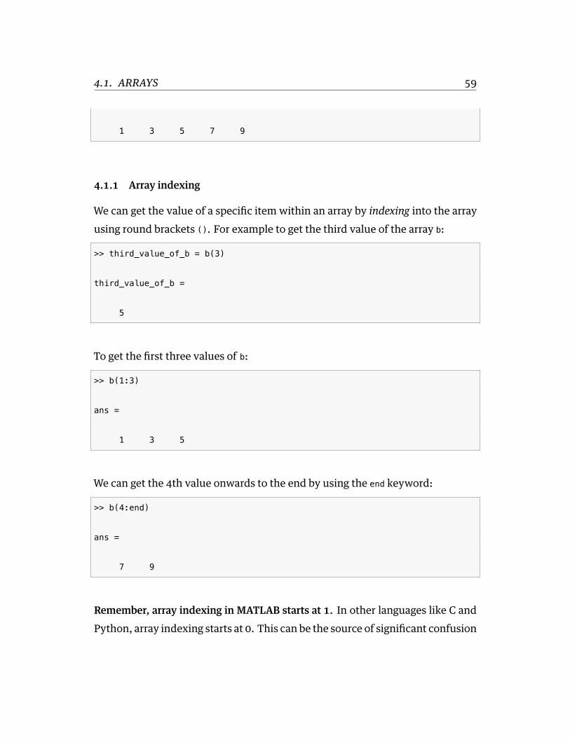
1 3 5 7 9
4.1.1 Array indexing
We can get the value of a specific item within an array by indexing into the arrayusing round brackets (). For example to get the third value of the array b:
>> third_value_of_b = b(3)
third_value_of_b =
5
To get the first three values of b:
>> b(1:3)
ans =
1 3 5
We can get the 4th value onwards to the end by using the end keyword:
>> b(4:end)
ans =
7 9
Remember, array indexing in MATLAB starts at 1. In other languages like C andPython, array indexing starts at 0. This can be the source of significant confusion
4.1. ARRAYS 60
when translating code from one language into another.
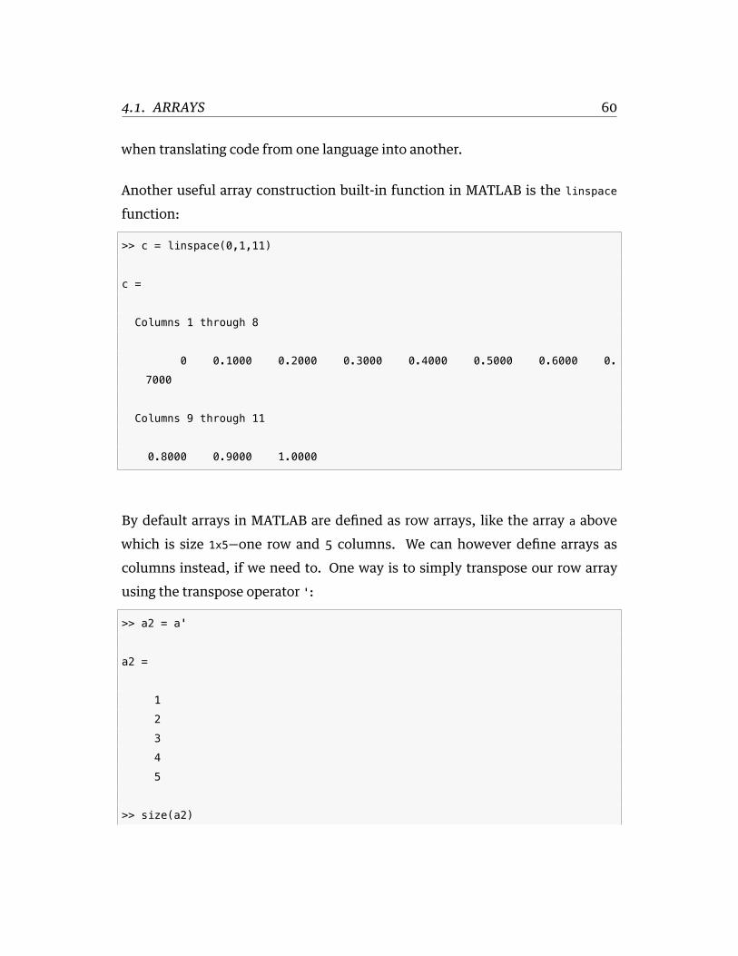
Another useful array construction built-in function in MATLAB is the linspace
function:
>> c = linspace(0,1,11)
c =
Columns 1 through 8
0 0.1000 0.2000 0.3000 0.4000 0.5000 0.6000 0.
7000
Columns 9 through 11
0.8000 0.9000 1.0000
By default arrays in MATLAB are defined as row arrays, like the array a abovewhich is size 1x5—one row and 5 columns. We can however define arrays ascolumns instead, if we need to. One way is to simply transpose our row arrayusing the transpose operator ':
>> a2 = a'
a2 =
1
2
3
4
5
>> size(a2)

4.1. ARRAYS 61
ans =
5 1
Now we can see a2 is a 5x1 column array.
We can directly define column arrays using the semicolon ; notation instead ofcommas or spaces, like so:
>> a2 = [1;2;3;4;5]
a2 =
1
2
3
4
5
So in general, commasor spacesdenotemoving fromone column to another, andsemicolons denote moving from one row to another. This will become usefulwhen we talk about matrices (otherwise know as two-dimensional arrays).
4.1.2 Array sorting
MATLABhas abuilt-in function called sort() to sort arrays (andother structures).The algorithm used by MATLAB under the hood is the quicksort66 algorithm. Tosort an array of numbers is simple:
>> a = [5 3 2 0 8 1 4 8 5 6]
a =

4.1. ARRAYS 62
5 3 2 0 8 1 4 8 5 6
>> a_sorted = sort(a)
a_sorted =
0 1 2 3 4 5 5 6 8 8
If you give the sort function two output variables then it also returns the indicescorresponding to the sorted values of the input:
>> [aSorted, iSorted] = sort(a)
aSorted =
0 1 2 3 4 5 5 6 8 8
iSorted =
4 6 3 2 7 1 9 10 5 8
The iSorted array contains the indices into the original array a, in sorted order. Sothis tells us that the first value in the sorted array is the 4th value of the originalarray; the second value of the sorted array is the 6th value of the original array,and so on.
The default sort happens in ascending order. If we want to reverse this we canspecify this as an option to the sort() function:
>> sort(a, 'descend')

4.1. ARRAYS 63
ans =
8 8 6 5 5 4 3 2 1 0
4.1.3 Searching arrays
We can use MATLAB’s built-in function called find() to search arrays (or otherstructures) for particular values. So for example if we wanted to find all valuesof the above array a which are greater than 5, we could use:
>> ix = find(a > 5)
ix =
5 8 10
This tells us that the 5th, 8th and 10th values of a are greater than 5. If we wantto see what those values are, we index into a using those found indices idx:
>> a(ix)
ans =
8 8 6
We could combine these two steps into one line of code like this:
>> a(find(a>5))
ans =
8 8 6

4.1. ARRAYS 64
4.1.4 Array arithmetic
One great feature of MATLAB is that arithmetic (and many other) operations canbe carried out on an entire array at once—and what’s more, under the hood MAT-LAB uses optimized, compiled code to carry out these so-called vectorized oper-ations. Vectorized code is typically many times faster than the equivalent codeorganized in a naive way (for example using for-loops). We will talk about vec-torized code and other ways to speed up computation in Chapter 8.
We can multiply each element of the array a2 by a scalar value:
>> a2 * 5
ans =
5
10
15
20
25
We can perform a series of operations all at once:
>> a3 = (a2 * 5) + 2.5
a3 =
7.5000
12.5000
17.5000
22.5000
27.5000
These mathematical operations are performed elementwise, meaning element-

4.1. ARRAYS 65
by-element.
We can also perform arithmetic operations between arrays. For example let’s saywe wanted to multiply two 1x5 arrays together to get a third:
>> a = [1,2,3,4,5];
>> b = [2,4,6,8,10];
>> c = a*b
Error using *
Inner matrix dimensions must agree.
Oops! We get an error message. When you perform arithmetic operations be-tween arrays in MATLAB, the default assumption is that you are doing matrix(or matrix-vector) algebra, not elementwise operations. To force elementwiseoperations in MATLAB we use dot-notation:
>> c = a.*b
c =
2 8 18 32 50
Now the multiplication happens elementwise. Needless to say we still need thedimensions to agree. If we tried multiplying, elementwise, a 1x5 array with a 1x6
array we would get an error message:
>> d = [1,2,3,4,5,6];
>> e = c.*d
Error using .*
Matrix dimensions must agree.
>> size(c)

4.2. MATRICES 66
ans =
1 5
>> size(d)
ans =
1 6
4.2 Matrices
In mathematics a matrix is generally considered to have two dimensions: a rowdimension and a column dimension. We can define a matrix in MATLAB in thefollowing way. Here we define a matrix A that has two rows and 5 columns:
>> A = [1,2,3,4,5; 1,4,6,8,10]
A =
1 2 3 4 5
1 4 6 8 10
>> size(A)
ans =
2 5
We use commas (or we could have used spaces) to denote moving from columnto column, and we use a semicolon to denote moving from the first row to thesecond row.

4.2. MATRICES 67
If we want a 5x2 matrix instead we can either just transpose our 2x5 matrix:
>> A2 = A'
A2 =
1 1
2 4
3 6
4 8
5 10
Or we can define it directly:
>> A2 = [1,2; 2,4; 3,6; 4,8; 5,10]
A2 =
1 2
2 4
3 6
4 8
5 10
There are other functions in MATLAB that we can use to generate a matrix. Therepmat function in particular is useful when we want to repeat certain values andstick them into a matrix:
>> G = repmat([1,2,3],3,1)
G =
1 2 3
1 2 3

4.2. MATRICES 68
1 2 3
This means repeat the row vector [1,2,3] three times down columns, and onetime across rows. Here’s another example:
>> H = repmat(G,1,3)
H =
1 2 3 1 2 3 1 2 3
1 2 3 1 2 3 1 2 3
1 2 3 1 2 3 1 2 3
Now we’ve repeated the matrix G once down rows and three times acrosscolumns.
There are also special functions zeros() and ones() to create arrays or matricesfilled with zeros or ones:
>> I = ones(4,5)
I =
1 1 1 1 1
1 1 1 1 1
1 1 1 1 1
1 1 1 1 1
>> J = zeros(7,3)
J =
0 0 0
0 0 0

4.2. MATRICES 69
0 0 0
0 0 0
0 0 0
0 0 0
0 0 0
Of course we can fill a matrix with any value we want by multiplying a matrix ofones by a scalar:
>> P = ones(3,4) * pi
P =
3.1416 3.1416 3.1416 3.1416
3.1416 3.1416 3.1416 3.1416
3.1416 3.1416 3.1416 3.1416
If we use zeros or oneswith just a single input argument we end up with a squarematrix (same number of rows and columns):
>> Q = ones(5)
Q =
1 1 1 1 1
1 1 1 1 1
1 1 1 1 1
1 1 1 1 1
1 1 1 1 1
There is also a special MATLAB function called eye which will generate the iden-tity matrix (a special matrix in linear algebra sort of equivalent to the number 1

4.2. MATRICES 70
in scalar arithmetic):
>> eye(3)
ans =
1 0 0
0 1 0
0 0 1
4.2.1 Matrix indexing
We can index into a matrix using round brackets, just like with an array. Nowhowever we need to specify both a row and a column index. So for example theentry in the matrix A2 corresponding to the 3rd row and the second column is:
>> A2(3,2)
ans =
6
To get the value in the last row, and the first column:
>> A2(end,1)
ans =
5
We can also specify a range in our index values. So to get rows 1 through 3 andcolumns 1 through 2:

4.2. MATRICES 71
>> A2(1:3,1:2)
ans =
1 2
2 4
3 6
Wecanuse a shorthand for “all columns” (alsoworks for all rows) using the colonoperator:
>> A2(1:3,:)
ans =
1 2
2 4
3 6
We can use indexing to replace parts of a matrix. For example to replace the firstrow of A2 (which is presently [1 2] with [99 99] we could use this code:
>> A2(1,:) = [99 99]
A2 =
99 99
2 4
3 6
4 8
5 10
To replace the second column of A2 with 5 random numbers chosen from a gaus-
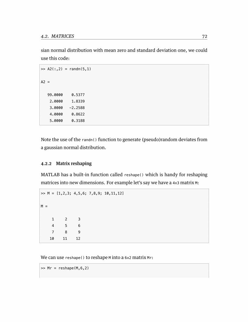
4.2. MATRICES 72
sian normal distribution with mean zero and standard deviation one, we coulduse this code:
>> A2(:,2) = randn(5,1)
A2 =
99.0000 0.5377
2.0000 1.8339
3.0000 -2.2588
4.0000 0.8622
5.0000 0.3188
Note the use of the randn() function to generate (pseudo)random deviates froma gaussian normal distribution.
4.2.2 Matrix reshaping
MATLAB has a built-in function called reshape() which is handy for reshapingmatrices into new dimensions. For example let’s say we have a 4x3 matrix M:
>> M = [1,2,3; 4,5,6; 7,8,9; 10,11,12]
M =
1 2 3
4 5 6
7 8 9
10 11 12
We can use reshape() to reshape M into a 6x2 matrix Mr:
>> Mr = reshape(M,6,2)

4.2. MATRICES 73
Mr =
1 8
4 11
7 3
10 6
2 9
5 12
Note that reshape() does its work by taking values columnwise from the originalinput matrix M. If we want to perform the reshaping in the other way—row-wise—we can do this by transposing the original matrix:
>> Mr2 = reshape(M',6,2)
Mr2 =
1 7
2 8
3 9
4 10
5 11
6 12
To reshape a matrix (or indeed any multi-dimensional array) into a column vec-tor, there is a convenient shorthand in MATLAB, namely the colon operator (:):
>> M_col = M(:)
M_col =
1
4

4.2. MATRICES 74
7
10
2
5
8
11
3
6
9
12
If we want a row vector instead we can just transpose the result:
>> M_row = M(:)'
M_row =
1 4 7 10 2 5 8 11 3 6 9 12
4.2.3 Matrix arithmetic
In MATLAB as with arrays, matrix–scalar operations happen elementwise,whereas matrix–matrix operations are assumed to be based on the rules of ma-trix algebra. We won’t go through matrix algebra in all its glory here, but you cansee a reminder of the basic operations on this wikipedia page:
Matrix Basic Operations67
I can recommend a great book on Linear Algebra by Gilbert Strang:
Introduction to Linear Algebra, 4th Edition68 by Gilbert Strang. Wellesley-Cambridge Press, 2009
He also has his course on MIT’s open-courseware, complete with videos for all

4.2. MATRICES 75
lectures here:
video lectures of Professor Gilbert Strang teaching 18.06 (Fall 1999)69
TheMathworkshas awebpagewith amatrix algebra “refresher” thatmight serveas a useful reminder for those who have had linear algebra in the past:
Matrix Algebra Refresher70
Here is an example of a scalar–matrix operation on our matrix A2 from above:
>> A2 * 10
ans =
10 20
20 40
30 60
40 80
50 100
Let’s say we wanted to multiply, elementwise, a 5x2 matrix A3 by A2:
>> A3 = rand(5,2)
A3 =
0.2785 0.9706
0.5469 0.9572
0.9575 0.4854
0.9649 0.8003
0.1576 0.1419
As with arrays, we can use dot notation to force elementwise multiplication:
>> A4 = A2 .* A3

4.2. MATRICES 76
A4 =
0.2785 1.9412
1.0938 3.8287
2.8725 2.9123
3.8596 6.4022
0.7881 1.4189
Without the dot notation we would get an error message:
>> A4 = A2 * A3
Error using *
Inner matrix dimensions must agree.
>> size(A2)
ans =
5 2
>> size(A3)
ans =
5 2
Toperformmatrixmultiplicationweneed a right-hand-side that has legal dimen-sions, in other words the same number of rows as A2 has columns. For example,if we have another matrix A5 sized 2x3:
>> A5 = rand(2,3)
A5 =

4.2. MATRICES 77
0.8147 0.1270 0.6324
0.9058 0.9134 0.0975
then we can perform matrix multiplication:
>> A6 = A2 * A5
A6 =
2.6263 1.9537 0.8274
5.2526 3.9075 1.6549
7.8789 5.8612 2.4823
10.5052 7.8150 3.3098
13.1315 9.7687 4.1372
Again, review your linear algebra if you have forgotten about the rules of matrixmultiplication. Just remember that to force elementwise operations, use dot-notation.
Addition and subtraction are always elementwise.
4.2.4 Matrix Algebra
As we saw above, MATLAB assumes that matrix–matrix operations are not ele-mentwise, but conform to the rules of linear algebra and matrix arithmetic. Theexception is matrix addition and subtraction, which happen elementwise evenin matrix algebra. Multiplication is special however, as we saw above.
What about division (/)? In MATLAB the so-called slash operator is the gatewayto much complexity.
>> help slash

4.2. MATRICES 78
Matrix division.
\ Backslash or left division.
A\B is the matrix division of A into B, which is roughly the
same as INV(A)*B , except it is computed in a different way.
If A is an N-by-N matrix and B is a column vector with N
components, or a matrix with several such columns, then
X = A\B is the solution to the equation A*X = B. A warning
message is printed if A is badly scaled or nearly
singular. A\EYE(SIZE(A)) produces the inverse of A.
If A is an M-by-N matrix with M < or > N and B is a column
vector with M components, or a matrix with several such columns,
then X = A\B is the solution in the least squares sense to the
under- or overdetermined system of equations A*X = B. The
effective rank, K, of A is determined from the QR decomposition
with pivoting. A solution X is computed which has at most K
nonzero components per column. If K < N this will usually not
be the same solution as PINV(A)*B. A\EYE(SIZE(A)) produces a
generalized inverse of A.
/ Slash or right division.
B/A is the matrix division of A into B, which is roughly the
same as B*INV(A) , except it is computed in a different way.
More precisely, B/A = (A'\B')'. See \.
./ Array right division.
B./A denotes element-by-element division. A and B
must have the same dimensions unless one is a scalar.
A scalar can be divided with anything.
.\ Array left division.
A.\B. denotes element-by-element division. A and B
must have the same dimensions unless one is a scalar.
A scalar can be divided with anything.
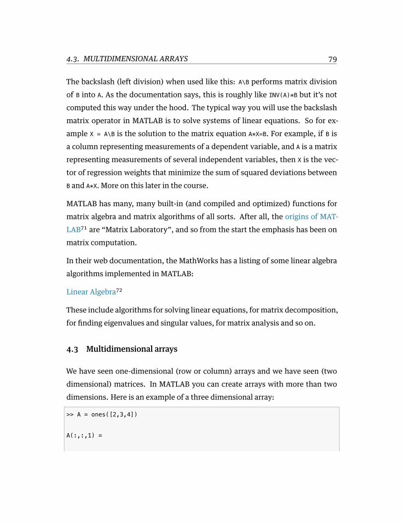
4.3. MULTIDIMENSIONAL ARRAYS 79
The backslash (left division) when used like this: A\B performs matrix divisionof B into A. As the documentation says, this is roughly like INV(A)*B but it’s notcomputed this way under the hood. The typical way you will use the backslashmatrix operator in MATLAB is to solve systems of linear equations. So for ex-ample X = A\B is the solution to the matrix equation A*X=B. For example, if B isa column representing measurements of a dependent variable, and A is a matrixrepresenting measurements of several independent variables, then X is the vec-tor of regression weights that minimize the sum of squared deviations betweenB and A*X. More on this later in the course.
MATLAB has many, many built-in (and compiled and optimized) functions formatrix algebra and matrix algorithms of all sorts. After all, the origins of MAT-LAB71 are “Matrix Laboratory”, and so from the start the emphasis has been onmatrix computation.
In their web documentation, the MathWorks has a listing of some linear algebraalgorithms implemented in MATLAB:
Linear Algebra72
These include algorithms for solving linear equations, for matrix decomposition,for finding eigenvalues and singular values, for matrix analysis and so on.
4.3 Multidimensional arrays
We have seen one-dimensional (row or column) arrays and we have seen (twodimensional) matrices. In MATLAB you can create arrays with more than twodimensions. Here is an example of a three dimensional array:
>> A = ones([2,3,4])
A(:,:,1) =
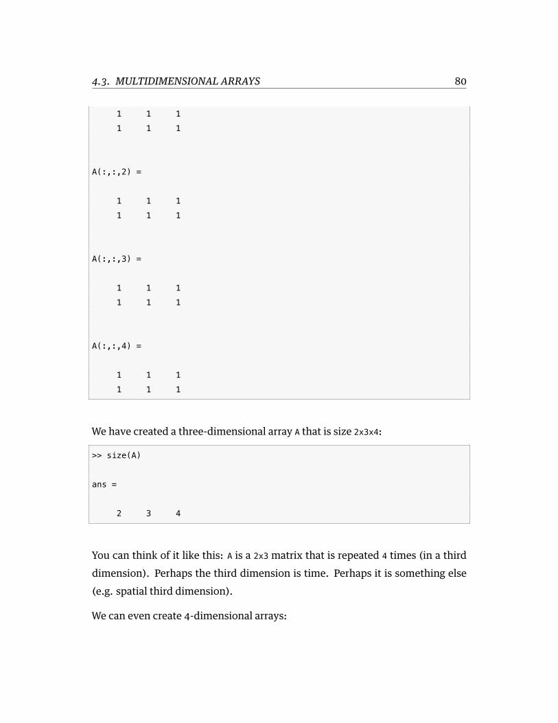
4.3. MULTIDIMENSIONAL ARRAYS 80
1 1 1
1 1 1
A(:,:,2) =
1 1 1
1 1 1
A(:,:,3) =
1 1 1
1 1 1
A(:,:,4) =
1 1 1
1 1 1
We have created a three-dimensional array A that is size 2x3x4:
>> size(A)
ans =
2 3 4
You can think of it like this: A is a 2x3 matrix that is repeated 4 times (in a thirddimension). Perhaps the third dimension is time. Perhaps it is something else(e.g. spatial third dimension).
We can even create 4-dimensional arrays:

4.3. MULTIDIMENSIONAL ARRAYS 81
>> B = rand(256,256,10,50);
>> whos
Name Size Bytes Class Attributes
B 4-D 262144000 double
>> size(B)
ans =
256 256 10 50
Here is a 4-dimensional array B. You can think of it as a 256x256x128 dimensional3D array repeated 50 times in a fourth dimension. Note how large the array is(262,144,000 bytes, about 250 megabytes). Depending on how much RAM youhave in your computer, you can potentially have MATLAB work with very largedata structures indeed.
A quick example, we could take the mean across the 4th dimension like so:
>> Bm = mean(B,4);
>> whos
Name Size Bytes Class Attributes
B 4-D 262144000 double
Bm 256x256x10 5242880 double
Anotheruseful function toknowabout is the squeeze() function inMATLAB.Thiswill remove any singleton dimensions—that is, dimensions that have size 1. Sofor example consider the following three-dimensional array:
>> A = reshape(1:12,[3,1,4])

4.3. MULTIDIMENSIONAL ARRAYS 82
A(:,:,1) =
1
2
3
A(:,:,2) =
4
5
6
A(:,:,3) =
7
8
9
A(:,:,4) =
10
11
12
>> size(A)
ans =
3 1 4

4.4. CELL ARRAYS 83
The second (middle) dimension is size 1, so we can use squeeze to reshape thisthree-dimensional array into a two-dimensional array of size [3x4]:
>> As = squeeze(A)
As =
1 4 7 10
2 5 8 11
3 6 9 12
>> size(As)
ans =
3 4
4.4 Cell arrays
Arrays (single-dimensional vectors as well as two-dimensional matrices andmulti-dimensional arrays) must contain values of the same type. MATLAB hasanother data structure called a cell array that allows one to store data of differenttypes in a structed similar to an array—namely it’s an indexed data container con-taining cells, and each cell can contain different data types. Cell arrays use curlybrackets instead of square brackets.
The MathWorks online documentation has a page devoted to cell arrays here:
Cell Arrays73
So for example we can create a cell array called myCell that contains 5 cells:
>> myCell = {1, 2, 3, 'hello', rand(1,10)}

4.4. CELL ARRAYS 84
myCell =
[1] [2] [3] 'hello' [1x10 double]
Cells 1 through 3 are numeric, cell 4 is a character string, and cell 5 is a [1x10]
array of double values. We can index into a cell array just like a regular array:
>> myCell{4}
ans =
hello
>> myCell{5}
ans =
Columns 1 through 8
0.7577 0.7431 0.3922 0.6555 0.1712 0.7060 0.0318 0.
2769
Columns 9 through 10
0.0462 0.0971
You can create an empty cell array like this:
>> emptyCell = {}
emptyCell =
{}

4.5. STRUCTURES 85
Or a cell array with a certain structure that is empty, like this:
>> emptyCell = cell(3,5)
emptyCell =
[] [] [] [] []
[] [] [] [] []
[] [] [] [] []
>> emptyCell{2,3} = 'hello'
emptyCell =
[] [] [] [] []
[] [] 'hello' [] []
[] [] [] [] []
4.5 Structures
MATLABhas another data type called a structure that is similar towhat youmighthave seen in other languages like Python, and is called a Dictionary. In MATLABa structure is an array with named fields that can contain any data type.
The MathWorks online documentation has a page devoted to structures here:
Structures74
Let’s create a structure called subject1 that contains a character string corre-sponding to their name, a numeric value corresponding to their age, a numericvalue correponding to their height, a value corresponding to the date the experi-ment was run, and an array corresponding to some recorded empirical data dur-ing an experiment:

4.5. STRUCTURES 86
>> subject1.name = 'Mr. T';
>> subject1.age = 63;
>> subject1.height = 1.78;
>> subject1.date = datetime(2015,08,12);
>> subject1.data = rand(100,2);
>> subject1.catchphrase = 'I pity the fool!';
>> subject1
subject1 =
name: 'Mr. T'
age: 63
height: 1.7800
date: [1x1 datetime]
data: [100x2 double]
catchphrase: 'I pity the fool!'
As you can see we use dot-notation to denote a field of a structure. As soon asyou introduce dot notation into a variable, it becomes a structure type. If a fieldwith the given name does not exist, it is created. Note the use of the datetime()
function which is a built-in function in MATLAB that handles dates and times.
We can access a field of a structure using dot-notation:
>> subject1.name
ans =
Mr. T
>> subject1.date
ans =

4.5. STRUCTURES 87
12-Aug-2015
4.5.1 Arrays of structures
We can of course form arrays of structures. An array can hold any data type aslong as each element is the same.
subject1.name = 'Mr. T';
subject1.age = 63;
subject1.height = 1.78;
subject1.date = datetime(2015,08,12);
subject1.data = rand(100,2);
subject1.catchphrase = 'I pity the fool!';
subject2.name = 'Polly Holliday';
subject2.age = 78;
subject2.height = [];
subject2.date = datetime(2015,08,12);
subject2.data = rand(100,2);
subject2.catchphrase = 'Kiss my grits!';
subject3.name = 'Leonard Nimoy';
subject3.age = 83;
subject3.height = [];
subject3.date = datetime(2015,02,26);
subject3.data = rand(100,2);
subject3.catchphrase = 'Live long and prosper';
allSubjects = [subject1, subject2, subject3];
>> allSubjects
allSubjects =

4.5. STRUCTURES 88
1x3 struct array with fields:
name
age
height
date
data
catchphrase
Nowwe cando convenient things like look at all of the agefields across thewholearray:
>> allSubjects.age
ans =
63
ans =
78
ans =
83
We can collect these into an array:
>> allAges = [allSubjects.age]
all_ages =

4.5. STRUCTURES 89
63 78 83
Orwe could collect all the datafields together into a three-dimensional array, andthen average across subjects:
>> allData = [allSubjects.data];
>> size(allData);
>> allData = [allSubjects.data];
>> size(allData)
ans =
100 6
>> allData = reshape(allData,100,2,3);
>> size(allData)
ans =
100 2 3
>> allDataMean = mean(allData,3);
>> size(allDataMean)
ans =
100 2
Note that if all elements of an array are not the same identical structure (i.e. donot have the same fields defined) then we get an error:
>> subject4.name = 'me'
subject4 =
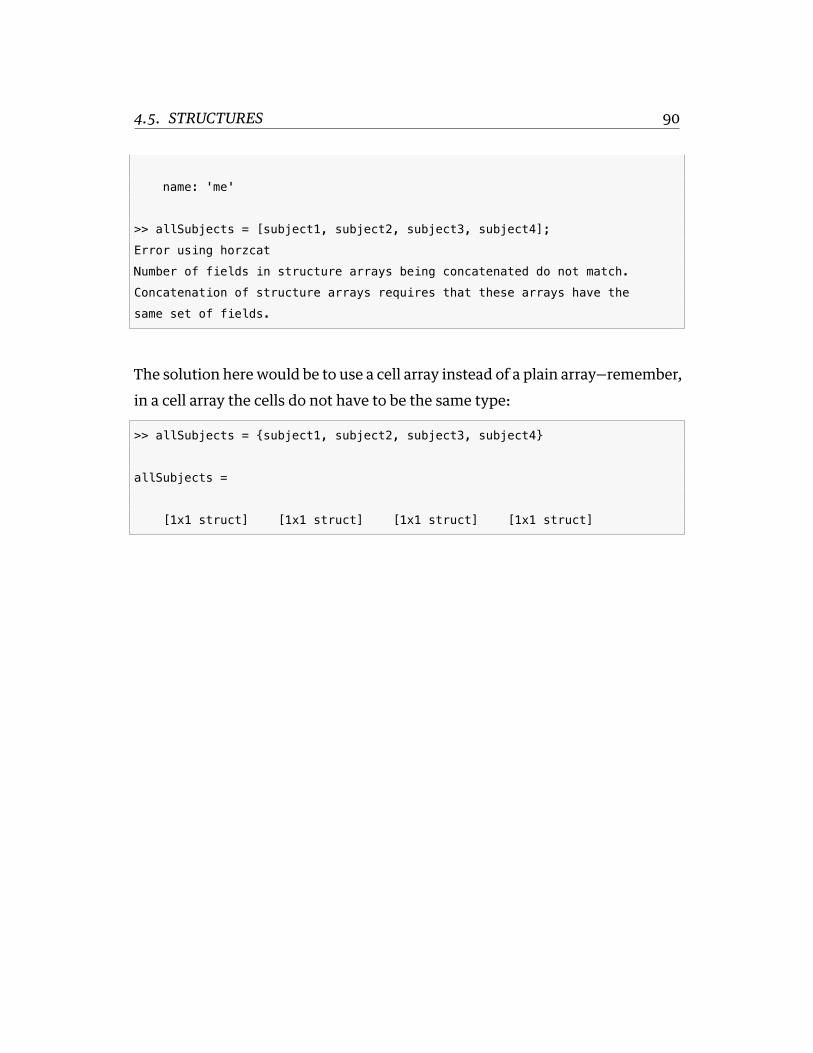
4.5. STRUCTURES 90
name: 'me'
>> allSubjects = [subject1, subject2, subject3, subject4];
Error using horzcat
Number of fields in structure arrays being concatenated do not match.
Concatenation of structure arrays requires that these arrays have the
same set of fields.
The solution here would be to use a cell array instead of a plain array—remember,in a cell array the cells do not have to be the same type:
>> allSubjects = {subject1, subject2, subject3, subject4}
allSubjects =
[1x1 struct] [1x1 struct] [1x1 struct] [1x1 struct]

4.5. STRUCTURES 91
Exercises
E 4.1 If we have a vector X containing n values, then the mean X is:
X =1n
N∑i=1
(Xi) (4.1)
In MATLAB there is a built-in function for computing the mean of a vector,called mean().
x = [2,1,5,4,8,3,4,3];
mean(x)
ans =
3.7500
Write a MATLAB script that computes the mean of a vector. Do it fromscratch, in other words don’t use the built-in function mean(). Ask the userto enter a vector using square brackets, and then compute the mean, andtell the user what it is. For example:
enter a vector, e.g. [3,1,4,1,5,9]: [1,2,3,4,5]
the mean of the vector is: 3.00
E 4.2 If we have a vector X containing n values, then the unbiased sample vari-ance75 s2 is:
s2 = 1n− 1
n∑i=1
(Xi − X)2 (4.2)
where X is the mean of the vector.

4.5. STRUCTURES 92
In MATLAB there is a built-in function for computing the variance of a vec-tor, called var().
x = [2,1,5,4,8,3,4,3];
var(x)
ans =
4.5000
Write aMATLAB script that computes theunbiasedvariance of a list of num-bers. Do it fromscratch, inotherwordsdon’tuse thebuilt-in functions var()or mean().
enter a vector, e.g. [3,1,4,1,5,9]: [1,2,3,4,5]
the variance of the vector is: 2.50

LINKS 93
Links
66https://en.wikipedia.org/wiki/Quicksort
67https://en.wikipedia.org/wiki/Matrix_(mathematics)#Basic_operations
68http://math.mit.edu/~gs/linearalgebra/
69http://ocw.mit.edu/courses/mathematics/18-06-linear-algebra-spring-2010/video-lectures/
70http://www.mathworks.com/help/finance/matrix-algebra-refresher.html
71http://www.mathworks.com/company/newsletters/articles/the-origins-of-matlab.
html
72http://www.mathworks.com/help/matlab/linear-algebra.html
73http://www.mathworks.com/help/matlab/cell-arrays.html
74http://www.mathworks.com/help/matlab/structures.html
75http://en.wikipedia.org/wiki/Variance#Sample_variance

LINKS 94

5 Control flow
Here we will learn above several ways to specify the flow of information as yourcode gets executed. We will learn about loops, which are constructs that allowyou to repeat blocks of code multiple times, typically while changing the valuesof variables inside the repeating block. We will learn about conditionals, whichallow you to execute different branches of code depending on the values of vari-ables. We will see how to pause your code, and to break out of a code block.
5.1 Loops
Loops are used when you have a chunk of code that you need to repeat over andover again, each time changing one (or more) parameters. Here is a simple ex-ample for the purposes of demonstration. Let’s say you want to load data from 5files, named data1.txt, data2.txt, …, data5.txt. Let’s say each file contains a one-dimensional array of 10 values. Let’s say you want to take the average of eachdata file and then report the overall mean and overall variance of those 5 values.Here’s one way to do it:
d1 = load('data1.txt');
d1m = mean(d1);
d2 = load('data2.txt');
d2m = mean(d2);
d3 = load('data3.txt');
d3m = mean(d3);
95

5.1. LOOPS 96
d4 = load('data4.txt');
d4m = mean(d4);
d5 = load('data5.txt');
d5m = mean(d5);
%
% report overall mean and overall variance of 5 data file means
alldata = [d1m d2m d3m d4m d5m];
datamean = mean(alldata);
datavar = var(alldata);
disp(sprintf('mean=%.3f and variance=%.3f', datamean, datavar))
You can see that there is a lot of repetition in this code. What if we had to loaddata from 1000 data files? There would be a lot of copying and pasting of codechunks. This is error prone and inefficient. Instead let’s use a for loop. A forloop allows you to repeat a block of code some predetermined number of times,and includes a counter so that you know which iteration of the loop is currentlyrunning. Here is what the code above would look like if we used a for loop:
nfiles = 5;
alldata = ones(1,nfiles)*NaN; % pre-allocate array and fill with NaN
for i=1:nfiles
d = load(['data',num2str(i),'.txt']);
alldata(i) = mean(d);
end
datamean = mean(alldata);
datavar = var(alldata);
disp(sprintf('mean=%.3f and variance=%.3f', datamean, datavar))
Nowall wewould need to change ifwe have 1000 data files (or onemillion) is thevalue of our variable nfiles=1000; or nfiles=1e6;—nothing else in the code wouldhave to change. This makes our code much more resilient against programmingerrors.

5.1. LOOPS 97
You can see a for loop begins with the keyword for followed by a name of a vari-able (your choice) that will keep track of which iteration of the loop is currentlyrunning. Then the equal sign = followed by a list of values to be iterated through.This list can be a constructed list using the colon operator (as in the exampleabove) or it can be a variable such as an array containing several values as in theexample below. Next is the block of code to be repeated. The end of this codeblock is denoted by the end keyword.
x = 1:3:15;
for i=x
disp(sprintf('i=%d', i))
end
which prints out:
i=1
i=4
i=7
i=10
i=13
For loops are executed in a serial fashion, one repetition after another. Whenwe talk later about parallel programming we will see that one can pretty easilyparallelize a for loop in MATLAB so that different iterations are distributed overmultiple cores of a CPU (or indeed over multiple CPUs in different machines overa network).
There is a second sort of loop called a while loop. This kind of loop is typicallyused when the number of iterations is not known in advance. A while loop keepsrepeating until the value of a logical expression changes from TRUE to FALSE(changes from 1 to 0). As a little demo, here is an example of a while loop that

5.1. LOOPS 98
prints out successive integers starting from 1, until they exceed a critical value,in this case 10:
i=1;
while (i<9)
disp(sprintf('i=%d', i))
i=i+1;
end
which displays:
i=1
i=2
i=3
i=4
i=5
i=6
i=7
i=8
The expression that determineswhether awhile loopwill continue repeating canbe any valid MATLAB expression that evaluates to 0 (FALSE) or 1 (TRUE). In fact,in MATLAB 0 is FALSE and any other value is considered to be TRUE.
For both for loops and while loops, there are two keywords to know about thatcan break you out of a loop (break) and can move you to the next iteration of theloop (continue). I tend not to use these, but you can see the MathWorks onlinehelp to read more about them:
break76
continue77

5.2. CONDITIONALS 99
5.2 Conditionals
So far we have seen how to use loops to repeat sections of code over and overagain as needed. The other major control flow mechanism in high-level lan-guages such as MATLAB is the conditional, which allows you to specify how codebranches in one direction or another depending on some logical condition.
So for example let’s say you ask the user to enter a number, and if the numberis even you output “The number is even.” and if the number is odd you output“The number is odd.”:
x = input('Enter a number: ');
if (mod(x,2)==0)
disp('The number is even.');
elseif (mod(x,2)~=0)
disp('The number is odd.');
end
which produces:
Enter a number: 15
The number is odd.
and
Enter a number: 12
The number is even.
In general one can string together any number of elseif branches (includingnone of them). For example:
x = input('Enter a number: ');
if (x<10)

5.3. SWITCH STATEMENTS 100
disp('The number is less than 10');
elseif (x<20)
disp('The number is less than 20');
elseif (x<30)
disp('The number is less than 30');
else
disp('I don''t have anything to say');
end
You don’t need any else statements at all if is suits your needs:
x = input('Enter a number: ');
if (x<0)
disp('That is a negative number');
end
The MathWorks online documentation has a page on conditional statementshere:
Conditional Statements78
5.3 Switch statements
The other type of conditional you might come across (though I rarely use them)is called a switch statement. Typically these are used when there is some rela-tively large list of potential cases and for each you have a defined (and different)course of action. Here is an example adapted from the MathWorks help page onconditionals:
d = input('Enter a day of the week: ','s');
switch d
case 'Monday'
disp('First day of the week')

5.4. PAUSE, BREAK, CONTINUE, RETURN 101
case 'Tuesday'
disp('Day 2')
case 'Wednesday'
disp('Day 3')
case 'Thursday'
disp('Day 4')
case 'Friday'
disp('Last day of the work week')
otherwise
disp('Weekend!')
end
Side note: can you spot any potential problem(s) with the above code?
5.4 Pause, break, continue, return
There are some keywords in MATLAB that give you finer control over the flow ofa program.
The pause keyword by itself will simply cause MATLAB to stop at that point inthe code, and wait until the user strikes any key—then MATLAB will continue.Try this:
for i=1:10
if (i==5)
disp('i is 5! hit any key to continue');
pause
else
disp(sprintf('i is not 5, continuing... (i is %d)', i));
end
end
which produces:

5.4. PAUSE, BREAK, CONTINUE, RETURN 102
i is not 5, continuing... (i is 1)
i is not 5, continuing... (i is 2)
i is not 5, continuing... (i is 3)
i is not 5, continuing... (i is 4)
i is 5! hit any key to continue
i is not 5, continuing... (i is 6)
i is not 5, continuing... (i is 7)
i is not 5, continuing... (i is 8)
i is not 5, continuing... (i is 9)
i is not 5, continuing... (i is 10)
The break keyword in MATLAB will terminate the execution of a loop. Any codeappearing after the break keywordwill not be executed. In nested loops the break
keyword only exits from the loop in which it appears. Here is an example of howbreak works:
for i=1:10
if (i==5)
disp('i is 5! stopping...');
break
else
disp(sprintf('i is not 5, continuing... (i is %d)', i));
end
end
which produces:
i is not 5, continuing... (i is 1)
i is not 5, continuing... (i is 2)
i is not 5, continuing... (i is 3)
i is not 5, continuing... (i is 4)
i is 5! stopping...

5.4. PAUSE, BREAK, CONTINUE, RETURN 103
I tend not to use break to exit out of loops but rather write code that more grace-fully determines what to do. It’s a personal preference.
The continue keyword passes control to the next iteration of a loop, and skips anycode appearing below where it appears. Like the break keyword, when continue
appears in nested loops it only applies to the loop in which it appears. Here is anexample of how continue works:
for i=1:10
if mod(i,2)==0
continue
end
disp(sprintf('the number %d is odd', i));
end
which produces:
the number 1 is odd
the number 3 is odd
the number 5 is odd
the number 7 is odd
the number 9 is odd
Again, I tend not to use continue but this is perhaps a personal preference.
The return keyword forces MATLAB to return control to the “invoking function”,whichmeans thatwhenusedwithin a function, returnwill exit the functionwith-out executing any of the remaining code. See Chapter 6 on Functions for moreabout how functions work in MATLAB.
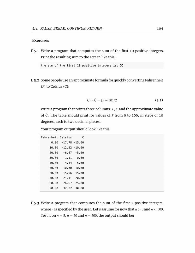
5.4. PAUSE, BREAK, CONTINUE, RETURN 104
Exercises
E 5.1 Write a program that computes the sum of the first 10 positive integers.Print the resulting sum to the screen like this:
the sum of the first 10 positive integers is: 55
E 5.2 Somepeopleuse anapproximate formula for quickly convertingFahrenheit(F) to Celsius (C):
C ≈ C = (F− 30)/2 (5.1)
Write a program that prints three columns: F, C and the approximate valueof C. The table should print for values of F from 0 to 100, in steps of 10degrees, each to two decimal places.
Your program output should look like this:
Fahrenheit Celsius C
0.00 -17.78 -15.00
10.00 -12.22 -10.00
20.00 -6.67 -5.00
30.00 -1.11 0.00
40.00 4.44 5.00
50.00 10.00 10.00
60.00 15.56 15.00
70.00 21.11 20.00
80.00 26.67 25.00
90.00 32.22 30.00
E 5.3 Write a program that computes the sum of the first n positive integers,where n is specified by the user. Let’s assume for now that n > 0 and n < 500.Test it on n = 5, n = 50 and n = 500, the output should be:

5.4. PAUSE, BREAK, CONTINUE, RETURN 105
the sum of the first 5 positive integers is: 15
the sum of the first 50 positive integers is: 1275
the sum of the first 500 positive integers is: 125250
E 5.4 Write a program to estimate the square root of 612 using Newton’smethod79. Write it so that the number whose square root is to be taken,and the number of iterations are both parameters (variables) that can beset by the user or the programmer. You can choose the initial guess on yourown, use whatever you like. I suggest the number 10.0 as in the wikipediaexample.
Find the square root of 612 using 5 iterations. Try it again using 10 itera-tions.

LINKS 106
Links
76http://www.mathworks.com/help/matlab/ref/break.html
77http://www.mathworks.com/help/matlab/ref/continue.html
78http://www.mathworks.com/help/matlab/matlab_prog/conditional-statements.html
79http://en.wikipedia.org/wiki/Newton's_method#Square_root_of_a_number
6 Functions
Functions areoneof themostuseful programming facilities that youwill run intobecause they allow you to make your code more modular.
6.1 Encapsulation
Wehave seen functions already, for example functions to print stuff to the screenlike disp() in MATLAB, functions for mathematics like sqrt(), and so on. Theadvantage of putting things like these into functions is that we avoid the need towrite everything from scratch each time we want to repeat a common operation.Imagine if every time we wanted to take the square root of a number, we had towrite an entire algorithm (like Newton’s method) to do so. It would be ridiculous.By encapsulating this operation into a function, all we need to do is write sqrt()
and the program goes and looks up the definition of that function, and executesthat code, without us having to type it in again, and again.
Herewewill be going throughhow towrite our own functions to encapsulate ourown operations, whatever they may be.
You can even imagine a series of functions that you write to perform the varioussteps of your data analysis, so that each time you collect more data in your exper-iment, you simply have to type:
>> go_my_analysis();
107

6.1. ENCAPSULATION 108
and all of your data analysis will be repeated, including the incorporation of anynewdata thatmaybe residing inyourdatadirectory. Of courseyouhave todefinewhat happens inside of go_my_analysis() for this to be useful. Maybe inside yourfunction you have defined other functions like:
>> load_all_data();
>> filter_data();
>> average_across_subjects();
>> perform_statistics();
>> generate_plots();
>> save_processed_data();
You get the idea.
Theother situationwheremodularity in your code is useful, is forwhenyouwantto share codewith other people (or use someone else’s code). If you (or someoneelse) has a specific input/output functionality in mind, then you can swap in andout one of many potential functions that claim to achieve the desired functional-ity, as long as it preserves the input/output relationship(s) that you specify.
For example, let’s say youdiscover that as part of your data analysis youwill needto compute the square root of a number, and let’s pretend that you don’t have afunction to do so built in to your language. (In fact you do of course—but forthe purpose of this thought experiment let’s imagine you don’t.) The input/out-put requirements for your square root function are that it takes as input a singlefloating-point number and returns a single floating point number. Now you cango shopping, among your friends, colleagues, or on the internet, for an imple-mentation of the square root function, and you can simply plug it in to your pro-gram and use it, as long as it takes a single floating-point number as input, andreturns a single floating-point number as output. This specification is sometimescalled the function prototype. Youmight find that several functions that youhave

6.2. FUNCTION SPECIFICATION 109
found work equally well in terms of returning the correct answer, but that one inparticular is way faster than the rest (perhaps it was written by a mathematicianwho knows some clever numerical tricks).
6.2 Function specification
In MATLAB usually sits in its own .m file, and starts with the word function, suchas in this file called mydeg2rad.m:
function radsOut = mydeg2rad(degIn)
% radsOut = mydeg2rad(degIn)
%
% accepts an angle in degrees and returns
% the equivalent in radians
%
conversion = pi / 180;
radsOut = degIn * conversion;
The first line of the file begins with the word function, followed by (1) outputvariable(s), (2) the function name, and (3) input variables. In the above casethere is a single output variablewhichwehave named radsOut, and a single inputvariable named degIn. A function in MATLAB can have zero, one, or more outputvariables, and zero, one or more intput variables.
Following the function protype on line 1, is a series of commented lines—linesbeginning with the % symbol. This tells MATLAB not to execute those lines asMATLAB code but that rather, these are human-readable comments. In additionnow when you type help mydeg2rad on the MATLAB command line, MATLAB willdisplay those comments as help for your function:

6.3. VARIABLE SCOPE 110
>> help mydeg2rad
radsOut = mydeg2rad(degIn)
accepts an angle in degrees and returns
the equivalent in radians
The last two lines of the file is where the work happens in the function. In thiscase our function has just two lines of code that do the work—but in general yourfunction can have many lines of code. The thing that your function has to have,is a definition of the value of the output variable(s)—the names of which are de-fined on line 1, in the function prototoype—so in our case this is a variable calledradsOut. This is how a function in MATLAB sends it output back to the code thatcalled the function.
We can use our function like this:
>> mydeg2rad(180)
ans =
3.1416
6.3 Variable scope
In MATLAB, we named the output variable(s) of our function and we also namedthe input variable(s) of our function. In the mydeg2rad function above, the outputvariable is named radsOut and the input variable is named degIn. The scope ofthese variable definitions is only within the function itself. Outside of the func-tion, MATLAB does not know about these variables.
Similarly, the conversion variable defined on the second-to-last line of the my-

6.3. VARIABLE SCOPE 111
deg2rad function also has a scope within the function itself, and outside of thefunction, MATLAB doesn’t know about it.
You can think of a function like a black box, and to the outside user, the innardsare unknown and inaccessible.
We can show this by trying to access the within-function variables:
>> mydeg2rad(180)
ans =
3.1416
>> degIn
Undefined function or variable 'degIn'.
>> radsOut
Undefined function or variable 'radsOut'.
>> conversion
Undefined function or variable 'conversion'.
If we want to collect the output of the function we have to define a new variableto hold it:
>> myValue = mydeg2rad(180)
myValue =
3.1416
Similarly, within a function, MATLAB does not know about variables outside ofthe function. So if we try to access, from within a function, variables defined
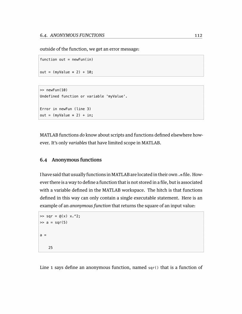
6.4. ANONYMOUS FUNCTIONS 112
outside of the function, we get an error message:
function out = newFun(in)
out = (myValue * 2) + 10;
>> newFun(10)
Undefined function or variable 'myValue'.
Error in newFun (line 3)
out = (myValue * 2) + in;
MATLAB functions do know about scripts and functions defined elsewhere how-ever. It’s only variables that have limited scope in MATLAB.
6.4 Anonymous functions
I have said thatusually functions inMATLABare located in their own .mfile. How-ever there is away to define a function that is not stored in a file, but is associatedwith a variable defined in the MATLAB workspace. The hitch is that functionsdefined in this way can only contain a single executable statement. Here is anexample of an anonymous function that returns the square of an input value:
>> sqr = @(x) x.^2;
>> a = sqr(5)
a =
25
Line 1 says define an anonymous function, named sqr() that is a function of

6.4. ANONYMOUS FUNCTIONS 113
one input variable which we shall call x (within the function—remember variablescope), and the output of that function ought to be x.ˆ2.
See the MATLAB documentation on anonyous functions for more details and ex-amples:
Anonymous Functions80

6.4. ANONYMOUS FUNCTIONS 114
Exercises
E 6.1 Write a function that determines whether a given number is a prime num-ber. Remember, a prime number81 is a (natural) number greater than 1 thatis only divisible (with zero remainder) by the number 1, and itself. The firstfew prime numbers are 2,3,5,7,11,13,17,19,23,29, …
For now you don’t have to implement a fancy algorithm for testing prime-ness (e.g. Sieve of Eratosthenes82). For now, it’s ok to implement a bruteforce method.
Hint: you will probably want to use the modulo83 operator to test whetherthe remainder is zero after dividing a number n by another number m. InMATLAB, modulo is achieved using a function mod(n,m).
So for example we can test whether the number 5 is prime by testingwhether (5 modulo m) equals 0 for m=2,3,4.
E 6.2 Write a function that computes the nth Fibonacci number84. Your functionshould be called fib() and should take as input a single integer value n, andshould return a single integer value representing the nth Fibonacci number.
Use a loop to accomplish this. Count how many arithmetic operations takeplace for computing the 10th Fibonacci number, and count also for the20th.
bonus: write a secondversionofyour function thatuses recursion85 insteadof a loop. Note how much more succint the code is. Count how many arith-metic operations take place for computing the 10th Fibonacci number, andfor the 20th as well. Now you see the potential downside of recursive algo-rithms.
bonus 2: incorporate memoization86 to make your recursive version moreefficient. Count again the number of arithmetic operations for the 10th and
6.4. ANONYMOUS FUNCTIONS 115
20th Fibonacci numbers.
E 6.3 The following equation can be used to estimate an approximate derivativeof a mathematical function f(x) if h is sufficiently small:
f′(x) ≈ f(x+ h)− f(x− h)2h (6.1)
Write a function numdiff(f,x,h) that returns an approximate estimate of thederivative of a mathematical function in a single variable x. Apply it tothe four mathematical functions given below to estimate derivatives at thegiven values:
1. f(x) = (ex) at x = 02. f(x) =
(e−2x2
)at x = 1
3. f(x) = (cos x) at x = π/24. f(x) = (ln x) at x = 1
Use h = 0.01
In each casewrite out the error, i.e., thedifferencebetween theexact deriva-tive and the result of the approximation. Use 10decimal places of precision.
If you need help finding out what the exact solutions to these derivativesare, (1) try to remember your calculus!, (2) ask a classmate, (3) google it, or(4) ask me (at which point I will direct you to WolframAlpha87).
hint: the ln() function (logarithm, base e) is typically called log() in pro-gramming languages like MATLAB whereas the logarithm, base 10 (typi-cally referred to in math class as log(), is typically called log10().
Here is some code scaffolding to get you started:
In a file called numdiff.m:
function out = numdiff(f,x,h)
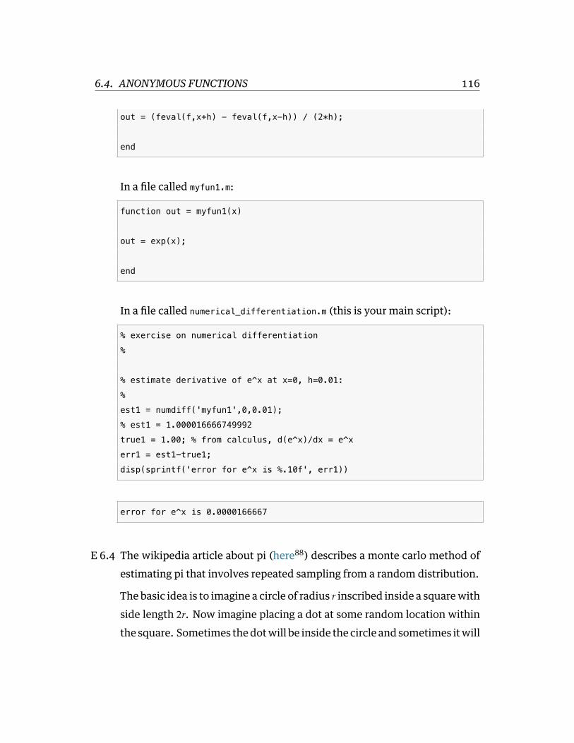
6.4. ANONYMOUS FUNCTIONS 116
out = (feval(f,x+h) - feval(f,x-h)) / (2*h);
end
In a file called myfun1.m:
function out = myfun1(x)
out = exp(x);
end
In a file called numerical_differentiation.m (this is your main script):
% exercise on numerical differentiation
%
% estimate derivative of e^x at x=0, h=0.01:
%
est1 = numdiff('myfun1',0,0.01);
% est1 = 1.000016666749992
true1 = 1.00; % from calculus, d(e^x)/dx = e^x
err1 = est1-true1;
disp(sprintf('error for e^x is %.10f', err1))
error for e^x is 0.0000166667
E 6.4 The wikipedia article about pi (here88) describes a monte carlo method ofestimating pi that involves repeated sampling from a random distribution.
The basic idea is to imagine a circle of radius r inscribed inside a squarewithside length 2r. Now imagine placing a dot at some random location withinthe square. Sometimes thedotwill be inside the circle and sometimes itwill

6.4. ANONYMOUS FUNCTIONS 117
not. If you count the number of dots that land inside the circle and dividethat by the total number of dots, that ratio ought to equal π
4 .
As an exercise, implement this method of estimating pi. Write the programso that you can use any number of random dots n. Start with 1000 dots andthen try larger numbers. See how close you can get to the actual value of π.Here are the first 100,000 digits89 of π.
Note that this algorithm isnot averyefficientor fastwayof getting thedigitsof π, but it’s a fun programming exercise nevertheless and a way to get youcoding.
hint: you will need a function that generates random numbers. In MATLABthe rand() function samples from a uniform (pseudo)random distributionover the interval (0, 1). Typing rand will return a single random value.
hint: to determine whether each point is inside or outside of the circle youcan compute the distance between the point and the centre of the circle. Ifthis distance is greater than the radius of the circle, it must be outside ofthe circle. Using the Pythagorean theorem90 you can easily show that theequation for the distance d between two points (x1, y1) and (x2, y2) is:
d =√
(x2 − x1)2 + (y2 − y1)2 (6.2)

LINKS 118
Links
80http://www.mathworks.com/help/matlab/matlab_prog/anonymous-functions.html
81http://en.wikipedia.org/wiki/Prime_number
82http://en.wikipedia.org/wiki/Sieve_of_Eratosthenes
83http://en.wikipedia.org/wiki/Modulo_operation
84http://en.wikipedia.org/wiki/Fibonacci_number
85http://en.wikipedia.org/wiki/Recursion_(computer_science)
86http://en.wikipedia.org/wiki/Memoization
87http://www.wolframalpha.com
88http://en.wikipedia.org/wiki/Pi#Geometry_and_trigonometry
89http://www.geom.uiuc.edu/~huberty/math5337/groupe/digits.html
90http://en.wikipedia.org/wiki/Pythagorean_theorem

7 Input & Output
Most of the time you will be writing programs that analyse data—whether thosedata are collected from experiments, or generated by models and simulations.We will need to be able to read in data from a file. It will also be useful to be ableto write data out to a file.
The MathWorks online documentation has a page devoted to importing and ex-porting data, here:
Data Import and Export91
Here we will go over how to read and write to some common types of files includ-ing ASCII files (plain text), MATLAB .mat files, as well as other binary formats.The MathWorks has a page listing all of the various file formats that MATLABknows how to import, it is quite lengthy:
Supported File Formats for Import and Export92
In general, there are two types of file formats, ASCII files (otherwise known asplain text files) and binary files. In fact, this is a lie and there really is only onefile type, namely binary files, since all data are ultimately stored as 0s and 1s(binary)—but we have conventions, like the ASCII code, which allow us to makeassumptions, to make life easier. So we know that if a (binary) file is coded usinga series of bytes, each of which corresponds to an ASCII code, then this file is infact a “plain text” or ASCII file (and you can read it using any plain text editorlike vim, emacs, sublime text, notepad, even MS Turd will open plain text files).
119

7.1. PLAIN TEXT FILES 120
Binaryfiles include things like image formats such as .png, .jpeg, soundfiles suchas .mp3 and video files such as .mp4 and .mov. Like I said before though, really, allfiles are binary. It’s just that we can open files containing ASCII code using manyprograms which know how to interpret the 0s and 1s as ASCII codes.
7.1 Plain text files
If your data are stored in a plan text file (ascii) then you can use the MATLABfunction load to load in the file. For example let’s say we have a plain text filecalled mydata.txt that contains the following:
2 3
4 5
6 7
8 9
Then we can use the load command to load the data:
>> d = load('mydata.txt');
>> whos
Name Size Bytes Class Attributes
d 4x2 64 double
>> d
d =
2 3
4 5
6 7
8 9

7.1. PLAIN TEXT FILES 121
You can also load the data without giving the load function an output variable tostore the data—in this case the datawill be stored in a newvariablewith the samename as the filename (but any file suffix, such as .txt stripped):
>> load mydata.txt
>> whos
Name Size Bytes Class Attributes
mydata 4x2 64 double
>> mydata
mydata =
2 3
4 5
6 7
8 9
For loading ASCII files, the file must contain a rectangular table of numbers, withan equal number of elements in each row. Delimiters such as spaces, commas,semicolons or tabs can be used—but they have to the same througout the file. Ifthese conditions are notmet, MATLABwill complain. For example if our data filemydata2.txt looks like this:
2 3
4 5
6 7 8
8 9
MATLAB will complain about number of columns not being the same:
>> load mydata2.txt

7.1. PLAIN TEXT FILES 122
Error using load
Number of columns on line 3 of ASCII file mydata2.txt must be the same as
previous lines.
To save data to an ASCII file, you can use the save command. For example let’ssay we have data store in a variable called data that looks like this:
data =
0.6557 0.7577
0.0357 0.7431
0.8491 0.3922
0.9340 0.6555
0.6787 0.1712
Then we can use save with the -ascii flag to save this into an ASCII file:
>> save mynewdata.txt data -ascii
The first argument (mynewdata.txt) is the filename of the new file to be created.The second argument (data) is the name of the variable to be saved to the file,and the third argument (-ascii) is a flag to the save command that tells MATLABto save the data in plain text (ASCII) format. Now if we look at the new file (forexamplebyopening it in theMATLAB text editor) thatwas created, mynewdata.txtit looks like this:
6.5574070e-01 7.5774013e-01
3.5711679e-02 7.4313247e-01
8.4912931e-01 3.9222702e-01
9.3399325e-01 6.5547789e-01
6.7873515e-01 1.7118669e-01
7.1. PLAIN TEXT FILES 123
Note how it has been saved in scientific notation.
If you want finer control over how things are stored in an ASCII file, you can read(as well as write) using lower-level control using MATLAB’s built-in functionsfprintf and fscanf. These mirror the functions with the same name that maybe familiar to you if you have programmed in C before. Here is an example ofwriting to an ASCII file where we want a very specific format:
data = [
0.6557 0.7577
0.0357 0.7431
0.8491 0.3922
0.9340 0.6555
0.6787 0.1712
];
fid = fopen('myfile.txt','w');
fprintf(fid, 'myfile.txt contains some data\n');
for i=1:size(data,1)
fprintf(fid,'item 1.1: %.4f, item 1.2: %.4f\n', data(i,1), data(i,2));
end
fprintf(fid, 'end of data\n');
fclose(fid);
This creates a file called myfile.txt that looks like this:
myfile.txt contains some data
item 1.1: 0.6557, item 1.2: 0.7577
item 1.1: 0.0357, item 1.2: 0.7431
item 1.1: 0.8491, item 1.2: 0.3922
item 1.1: 0.9340, item 1.2: 0.6555
item 1.1: 0.6787, item 1.2: 0.1712
end of data

7.2. BINARY FILES 124
7.2 Binary files
MATLAB has its own binary format for files, denoted using a .mat file suffix. Thesave and load functions in MATLAB with no other options use this default binaryformat. The advantage of MATLAB’s binary format over an ASCII format is (1)your data files will be smaller in size, and (2) with MATLAB’s .mat format you canstore more than one variable (and variables of different kinds) in a single file. Forexample here we store a scalar variable called mynumber, a vector called myvector,a matrix called mymatrix and a structure called mystructure in a single binary .mat
file called myfile.mat:
>> whos
Name Size Bytes Class Attributes
mymatrix 4x2 64 double
mynumber 1x1 8 double
mystructure 1x1 840 struct
myvector 1x7 56 double
>> save myfile mynumber myvector mymatrix mystructure
Now there is a file in my working directory called myfile.mat. I can now load thefile (and all the variables contained within it) into MATLAB’s memory using theload function. First I clear the memory to demonstrate that I’m not cheating:
>> clear
>> whos
Now I load the file:
>> load myfile
>> whos

7.3. ASCII OR BINARY? 125
Name Size Bytes Class Attributes
mymatrix 4x2 64 double
mynumber 1x1 8 double
mystructure 1x1 840 struct
myvector 1x7 56 double
7.3 ASCII or binary?
The question of which file format to use as you go forward and write programsfor analysing your data is an interesting one to consider. For long-term archivalpurposes, I would suggest storing your data in an ASCII format, so that it remainsreadable by human eyes. There will always be programs to read ASCII files. Therisk of storing data in a binary format is that (a) whatever program you used tosave the data will no longer be easily accessible in the future, and/or (b) you maynot even remember what the binary format is. The disadvantage of storing datain ASCII format is that the files will be larger than if they were stored in a binaryformat. The availability and affordability of large amounts of storage is growingso quickly however, so perhaps one does not have to worry too much about this.

LINKS 126
Links
91http://www.mathworks.com/help/matlab/data-import-and-export.html
92http://www.mathworks.com/help/matlab/import_export/supported-file-formats.
html

8 Debugging, profiling and speedy code
In this chapter we will look at ways of solving problems with your code using thevarious debugging tools in MATLAB. We will also look at profiling your code us-ing the built-in profiler in MATLAB, which can be used to identify parts of yourcode that are taking the most time to execute. We will go over a number of waystomake sure your code runs fast. In some cases this amounts to telling you aboutwhat not to do to make your code run slow. Finally we will look at the MATLABCoder, which is a toolbox included in MATLAB that can generate standalone CandC++code fromMATLABcode. It canalsogenerate so-calledbinaryMEXfunc-tions that allow you to call compiled versions of your MATLAB code, potentiallyspeeding up computations.
8.1 Debugging
There are at least two kinds of errors you will encounter in programming. Thefirst is when you run your code and it aborts because of some kind of error, andyou recieve an error message. Sometimes those error messages are useful andyou can determine immediately what is wrong. Other times the error message iscryptic and it takes some detective work on your part to figure out what part ofthe code is failing, and why it is failing.
The second type of error is when your code runs without aborting, and withoutreporting any problem to you, but you do not get the expected result. This is
127

8.1. DEBUGGING 128
much more difficult to debug.
In general the approach you should use for debugging is to step through yourcode, line by line, and ensure that each step is (a) performing the operation youthink it is, and (b) is performing the appropriate operation.
Thebuilt-inMATLABeditor that you canuse to edit yourMATLABcodefiles has ahandy feature called breakpoints that allows you to set a breakpoint (or multiplebreakpoints) on a specific line (or lines) of your code, such that as you run yourcode, MATLAB stops at a breakpoint and enters a special mode called the debug-ger. Once in the debugger you can examine values of variables, step to the nextline of code, step in or out of functions, and continue executing the rest of thecode. It’s a very useful way to halt execution at specific places in your code, sothat you can examinewhat is going on. Often this is howwill find bugs and errorsin your code—when you assumed a variable had a specific value, or an operationresulted in a specific value, and in fact it didn’t.
Here is an example of a MATLAB script called go.mwhich computes some values,andexecutes a for–loop inwhich is fills a vector vwith somenumbers. By clickingwith the mouse on the little dash (-) next to the line number 7 (on the left handside of the editor window) I have inserted a breakpoint, which appears as a filledred circle. Figure 8.1 shows what this looks like.
Now when we run the program, MATLAB stops the first time it encounters thebreakpoint on line 7. You will see this at the MATLAB command prompt:
>> go
7 d = c / 12;
K>>
It reports the line number (7) and the code appearing on that line, and it putsyou in to debugger mode, as indicated by the prompt K>>. Now you can enter the

8.1. DEBUGGING 129
Figure 8.1: Setting a breakpoint at line 7.
names of variables to query their value, for example we can see what the valueof i, and c are:
K>> i
i =
1
K>> c
c =
30

8.1. DEBUGGING 130
We can step to the next line of code by clicking on the “Step” button appearingat the top of the editor window, as shown in Figure 8.2.
Figure 8.2: Stepping to the next line of code.
You will see that there is now a little green arror pointing to the right, at line 8 inthe code. This indicates the line of code where the debugger has stopped, and iswaiting for you to tell itwhat to donext. We can click on the “Continue” button atthe top of the editor window to continue. When we do this we see that MATLABhas stopped again, at line 7 again, as shown in Figure 8.3.
At the command prompt we can enter i to query the value of i and we see thatindeed we are now at iteration 2 of the for–loop:
K>> i
i =
2

8.1. DEBUGGING 131
Figure 8.3: After continuing code execution.
If we click “Continue” again we will stop again at line 7, at the third iteration ofthe for–loop, and so on. To continue without stopping at the breakpoint eachtime, we need to remove or disable the breakpoint. Right-click on the little redcircle and a pop-up menu gives you these options. Note that there is also an op-tion called “Set/Modify Condition...”—this allows you to specify a logical condi-tion which if true, will cause MATLAB to stop at the breakpoint, otherwise not.This is a nice way to set up breakpoints that only stop the code if certain condi-tions are met—for example if the value of a variable you know should never benegative, is less than zero.
The MathWorks online documentation has a page devoted to debugging here:
Debugging93

8.2. TIMING AND PROFILING 132
Figure 8.4: Setting a conditional breakpoint.
8.2 Timing and Profiling
One obvious way of speeding up your MATLAB programs is to first identify thepieces of your program that are slowest—and then do what you can to speed upthose parts.
8.2.1 Timing your code using tic and toc
One way to time your code is to use the tic and toc commands in MATLAB.
>> help tic
tic Start a stopwatch timer.
tic and TOC functions work together to measure elapsed time.
tic, by itself, saves the current time that TOC uses later to
measure the time elapsed between the two.

8.2. TIMING AND PROFILING 133
TSTART = tic saves the time to an output argument, TSTART. The
numeric value of TSTART is only useful as an input argument
for a subsequent call to TOC.
Example: Measure the minimum and average time to compute a sum
of Bessel functions.
REPS = 1000; minTime = Inf; nsum = 10;
tic;
for i=1:REPS
tstart = tic;
sum = 0; for j=1:nsum, sum = sum + besselj(j,REPS); end
telapsed = toc(tstart);
minTime = min(telapsed,minTime);
end
averageTime = toc/REPS;
See also toc, cputime.
Reference page in Help browser
doc tic
>> help toc
toc Read the stopwatch timer.
TIC and toc functions work together to measure elapsed time.
toc, by itself, displays the elapsed time, in seconds, since
the most recent execution of the TIC command.
T = toc; saves the elapsed time in T as a double scalar.
toc(TSTART) measures the time elapsed since the TIC command that
generated TSTART.
Example: Measure the minimum and average time to compute a sum

8.2. TIMING AND PROFILING 134
of Bessel functions.
REPS = 1000; minTime = Inf; nsum = 10;
tic;
for i=1:REPS
tstart = tic;
sum = 0; for j=1:nsum, sum = sum + besselj(j,REPS); end
telapsed = toc(tstart);
minTime = min(telapsed,minTime);
end
averageTime = toc/REPS;
See also tic, cputime.
Reference page in Help browser
doc toc
The typical pattern using tic and toc is to bracket a chunk of code you want totime with tic and toc. There are several examples in section 8.3 below in whichtic and toc are used to time MATLAB code execution time.
8.2.2 Using MATLAB Profiler
There is a tool inMATLABcalled theProfiler that is very useful for showingwhichparts of your program take the most amount of time to execute. Think of the pro-filer as a way of automatically timing every part of your program and generatinga handy report (which it does also).
The basic way to use the profiler is to first activate it by typing:
>> profile on
You can then run your MATLAB script, and once it is finished, stop the profiler

8.2. TIMING AND PROFILING 135
by typing:
>> profile off
You can then generate a report by typing:
>> profile report
Here is an example using a script called go.m which calls two other functions, my-fun1 and myfun2:
n = 1e4;
m = zeros(100,100);
for i=1:n
m = m + myfun1(m);
m = m + myfun2(m);
end
disp(sprintf('grand mean of m is %.6f\n', mean(m(:))/n));
function out = myfun1(in)
[r,c] = size(in);
tmp = randn(r,c);
for i=1:r
for j=1:c
tmp(i,j) = sqrt(tmp(i,j));
end
end
out = tmp;
end
function out = myfun2(in)
[r,c] = size(in);
tmp = randn(r,c);

8.2. TIMING AND PROFILING 136
tmp = sqrt(tmp);
out = tmp;
end
We turn on the profiler, run the code, stop the profiler, and generate a report,which is shown in Figure 8.5.
Figure 8.5: Profiler report of go.m.
We can see that the go script overall took 160.726 seconds to run. We also seea list of functions that were called within go, and the time they took. We cansee immediately that myfun1 is way slower than myfun2. If we click the mouse onmyfun1 in the report, we get a new report of the myfun2 function itself, which isshown in Figure 8.6.
We get a quite detailed report of the lines of the code where the most time wasspent. We also see the time spent, and the number of calls made to each line of
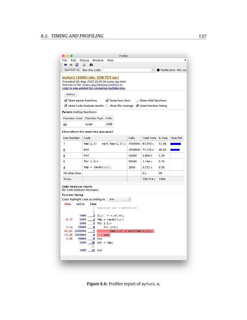
8.2. TIMING AND PROFILING 137
Figure 8.6: Profiler report of myfun1.m.

8.3. SPEEDY CODE 138
code in the function.
In this case we see that line 7 of the myfun1 function is taking a lot of time toexecute—this is where we take the square root of each element of a large ma-trix, within two nested for–loops. Line 7 represents the innermost part of thesetwo nested for–loops, and so it’s no surprise that we are spending a lot of timehere. See section 8.3.2 below for more information about how to avoid nestedfor–loops by using vectorized code operations.
The other way of running the profiler is by clicking with your mouse on the “Runand Time” button in the toolbar of the MATLAB code editor. The profiler will runyour code, timing each line, and will open up a report window.
The MathWorks online documentation has a page on the profiler here:
Profiling for Improving Performance94
8.3 Speedy Code
8.3.1 Array preallocation
There are many cases in which we want to collect the results of many computa-tions together into a single data structure, e.g. a vector or array. Onewayof doingthis is to start with an empty array, and each time through the loop, add a valueto it (and hence lengthening it). It turns out this way is very slow. What’s much,much faster is to pre-allocate the array (and fill it with whatever values you want,e.g. 0s, or NaNs), and then set each value as you go through the loop to the resultof your computation.
Here is an example in MATLAB:
% let's compute the following formula
% for values between 0 and n:
%

8.3. SPEEDY CODE 139
% f(i) = (i + f(i-1)) / n
n = 1e5;
% the slow way:
%
tic
c = [0];
for i=2:n
c = [c, (i + c(i-1)) / n];
end
toc
%
% on my laptop this takes 3.605413 seconds
% the fast way, with array pre-allocation
%
tic
c = zeros(1,n);
for i=2:n
c(i) = (i + c(i-1)) / n;
end
toc
%
% on my laptop this takes 0.002819 seconds
% this is over 1,000 times faster than the slow version
In the slowversion,we startwith an array of length 1 containing thenumber zero.Each time through the loop we concatenate the array with the next value, and inthis way we build up the array.
In the fast version, we pre-allocate an array of the required length, fill it with 0s,and then each time through the loop we simply assign the appropriate value tothe appropriate array position.

8.3. SPEEDY CODE 140
The reason the slowversion is so slow, is that each timewe concatenate the array,several steps take place under the hood:
1. a block of memory large enough to hold a new array (of length: one greaterthan the old array) is found and reserved
2. the new array is created3. the old array is copied into all elements of the new array (except the last
element which is left empty)4. the new value is copied to the last value in the new array5. the memory assigned to the old array is freed up (no longer reserved)
As you can imagine, when the array gets large, the copy operation can take a lotof time. It’s inefficient to keep copying the array over and over again.
With pre-allocation, there is no copying, only assignment, and only single valuesare assigned.
8.3.2 Vectorization
Many functions in MATLAB are vectorized, that is, they can operate on arraysand matrices as if the function had been applied one by one to each element. Anexample is the sqrt() function.
Here’s an example where we have three long arrays, defining 3D points, and ourtask is compute the length of each vector. We first compute the vector lengthsthe slowway, using a straightforward for–loop. We thendo the same calculationsbut in a vectorized fashion—in this case by recognizing that arithmetic operationssuch as squaring, addition and taking the square root can all be applied to vectorsas a whole, and MATLAB performs these operations in a vectorized fashion.
n = 1e7; % a big number
x = rand(1,n); % array of random numbers
y = rand(1,n); % array of random numbers

8.3. SPEEDY CODE 141
z = rand(1,n); % array of random numbers
% compute the norm of the 3-D vectors (x,y,z)
% the slow way
%
tic
norm_slow = zeros(1,n); % pre-allocate array
for i=1:n
norm_slow(i) = sqrt(x(i)^2 + y(i)^2 + z(i)^2);
end;
toc
%
% on my laptop this takes 0.594378 seconds
% the vectorized way
%
tic
norm_slow = sqrt(x.^2 + y.^2 + z.^2);
toc
%
% on my laptop this takes 0.040536 seconds
% this is about 15 times faster than the slow version
When we implement this in a vectorized way, MATLAB uses pre-compiled, opti-mized functions to execute that part of the code, instead of running it throughthe interpreter. When we use a for–loop, everything happens at the interpreterlayer.
Two aspects of the code example are vectorized. First, weuse the exponent oper-ator in MATLAB on the entire vector x, y, and z (with the dot notation to denoteelement-by-element exponentiation). This exponentiates the entire vector usingprecompiled optimized code under the hood. Then we use the sqrt() function

8.3. SPEEDY CODE 142
which also takes the whole array as an argument. Again, optimized precompiledcode is used on the entire array rather than stepping through the array in a forloop, at the interpreter level.
Another salient example of vectorization is matrix algebra. The matrix alge-bra operators (e.g. matrix multiplication) make use of highly optimized, pre-compiled routines that areway faster thandoing things byhandat the interpreterlevel, using for loops. Here is an example in code:
% matrix multiplication
%
A = rand(400,500);
B = rand(500,600);
C = zeros(400,600);
% the slow way, using for loops at the interpreter level
%
tic
m = size(A,1);
n = size(A,2);
p = size(B,1);
q = size(B,2);
for i=1:m
for j=1:q
the_sum = 0;
for k=1:p
the_sum = the_sum + A(i,k)*B(k,j);
end
C(i,j) = the_sum;
end
end
toc
%
% on my laptop this takes 2.552810 seconds

8.3. SPEEDY CODE 143
% the fast way (vectorized)
%
C = zeros(400,600);
tic
C = A*B;
toc
%
% on my laptop this takes 0.001998 seconds
% this is over 1,000 times faster than the slow version
When we write A*B in MATLAB, where A and B are both matrices, MATLAB usesprecompiled, optimized linear algebra routines (written in C and compiled foryour CPU) to perform the matrix multiplication calculation.
8.3.3 Suppress output to the screen
This one might seem obvious, but if you are doing something thousands or mil-lions of times, and each time you print something to the screen, that will slowdown your code. Here’s an example:
% suppress output!
% slow version
%
n = 1e5;
x = zeros(1,n);
tic
for i=1:n
tmp = (i*i) + (i/2)
x(i) = tmp;
end
toc
%
% on my laptop this takes 2.571819 seconds

8.3. SPEEDY CODE 144
% fast version
%
x = zeros(1,n);
tic
for i=1:n
tmp = (i*i) + (i/2);
x(i) = tmp;
end
toc
%
% on my laptop this takes 0.001080 seconds
% this is more than 2,000 times faster than the slow version
The only difference between the two version of this for–loop is that in the first,we fail to suppress output to the screen when we define the tmp variable. In thesecond version we include a semicolon to suppress output to the screen and ourcode runs more than 2,000 times as fast. Semicolons are powerful!
Printing values to the screen within a for–loop is not always a bad thing however.Often we want to print values to the screen in a for–loop so that we can keeptrack of how far along the computation is, or detect errors. One alternative thatavoids the slow execution of printing to the screen every time through the loop,is to print more sporadically. Here is an example where we repeat the above codebut we only print to the screen every 10,000 iterations. This still allows you tomonitor the progress of the computation, but it doesn’t eat up precious time dis-playing stuff on the screen every single time through the loop:
% partial suppression of output
% slow version
%
n = 1e6;

8.3. SPEEDY CODE 145
x = zeros(1,n);
tic
for i=1:n
tmp = (i*i) + (i/2);
x(i) = tmp;
disp(tmp);
end
time1=toc
%
% on my laptop this takes 7.689031 seconds
% fast version
%
x = zeros(1,n);
tic
for i=1:n
tmp = (i*i) + (i/2);
x(i) = tmp;
if (mod(i,100000)==0)
disp(tmp);
end
end
time2=toc
%
% on my laptop this takes 0.063113 seconds
% this is still more than 100 times faster than the slow version
%
disp(sprintf('time1=%.6f, time2=%.6f\n', time1, time2))
8.3.4 Overhead cost of calling a function
We’ve talked about the benefits of modularizing your code, and sticking com-monlyusedoperations inside functions. This is absolutely a good idea. It isworth

8.3. SPEEDY CODE 146
notinghowever that the act of calling a functiondoes involve someoverhead costin time (and in memory), for various things that happen under the hood.
Functions in general are a very good idea, but if youput everything into functions,you can start to experience unneccessary slowdowns due to the overhead in call-ing functions, passing parameters in, and passing results out. Here is a simpleexample in which we loop through an array and perform a number of calcula-tions on each element. In the slow version we put every single calculation intoits own function (admittedly this is a bit extreme, but it illustrates the problem).In the fast version we don’t use functions at all:
% slow version: make everything a function!!
%
n = 1e6;
a = 1:n;
tic
for i=1:n
tmp1 = mycomp1(i);
tmp2 = mycomp2(i);
tmp3 = mycomp3(i);
tmp4 = mycomp4(i);
tmp5 = mycomp5(i);
a(i) = tmp1 + tmp2 + tmp3 + tmp4 + tmp5;
end
toc
%
% on my laptop this takes 1.048836 seconds
% fast version: no functions here
%
n = 1e6;
a = 1:n;
tic
for i=1:n

8.3. SPEEDY CODE 147
tmp1 = i*1;
tmp2 = i*2;
tmp3 = i*3;
tmp4 = i*4;
tmp5 = i*5;
a(i) = tmp1 + tmp2 + tmp3 + tmp4 + tmp5;
end
toc
%
% on my laptop this takes 0.010898 seconds
% this is about 100 times faster than the slow version
In this case we have defined five functions in separate .m files (mycomp1.m, my-
comp2.m, mycomp3.m, mycomp4.m, mycomp5.m,):
function out = mycomp1(in)
out = in*1;
function out = mycomp2(in)
out = in*2;
function out = mycomp3(in)
out = in*3;
function out = mycomp4(in)
out = in*4;
function out = mycomp5(in)
out = in*5;
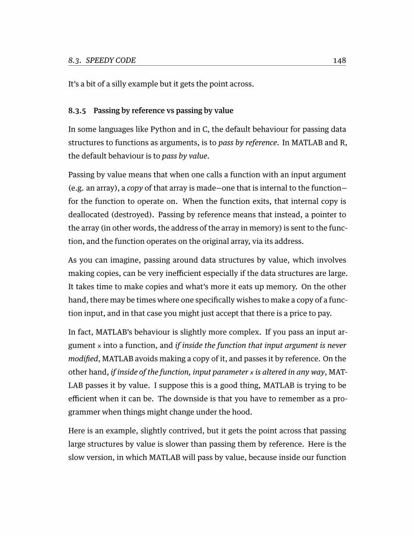
8.3. SPEEDY CODE 148
It’s a bit of a silly example but it gets the point across.
8.3.5 Passing by reference vs passing by value
In some languages like Python and in C, the default behaviour for passing datastructures to functions as arguments, is to pass by reference. In MATLAB and R,the default behaviour is to pass by value.
Passing by value means that when one calls a function with an input argument(e.g. an array), a copy of that array is made—one that is internal to the function—for the function to operate on. When the function exits, that internal copy isdeallocated (destroyed). Passing by reference means that instead, a pointer tothe array (in other words, the address of the array in memory) is sent to the func-tion, and the function operates on the original array, via its address.
As you can imagine, passing around data structures by value, which involvesmaking copies, can be very inefficient especially if the data structures are large.It takes time to make copies and what’s more it eats up memory. On the otherhand, there may be times where one specifically wishes to make a copy of a func-tion input, and in that case you might just accept that there is a price to pay.
In fact, MATLAB’s behaviour is slightly more complex. If you pass an input ar-gument x into a function, and if inside the function that input argument is nevermodified, MATLAB avoids making a copy of it, and passes it by reference. On theother hand, if inside of the function, input parameter x is altered in any way, MAT-LAB passes it by value. I suppose this is a good thing, MATLAB is trying to beefficient when it can be. The downside is that you have to remember as a pro-grammer when things might change under the hood.
Here is an example, slightly contrived, but it gets the point across that passinglarge structures by value is slower than passing them by reference. Here is theslow version, in which MATLAB will pass by value, because inside our function

8.3. SPEEDY CODE 149
we are changing a value of the input parameter x:
function out = myfunc_slow(x,y)
tmp = x(1);
x(1) = tmp*2;
out = tmp;
andhere is the fast version,wherewedon’t change thevalueof x, andsoMATLABwill pass by reference:
function out = myfunc_fast(x,y)
tmp = x(1);
y(1) = tmp*2;
out = tmp;
Here we demonstrate the speed difference:
x = rand(1e4,1e4);
y = [1,2,3];
% the slow way
% MATLAB passes x by value
% because it is altered inside myfunc_slow()
%
tic
for i=1:20
o1 = myfunc_slow(x,y);
end
toc
%
% on my laptop this takes 8.557641 seconds
% the fast way
% MATLAB passes x by reference
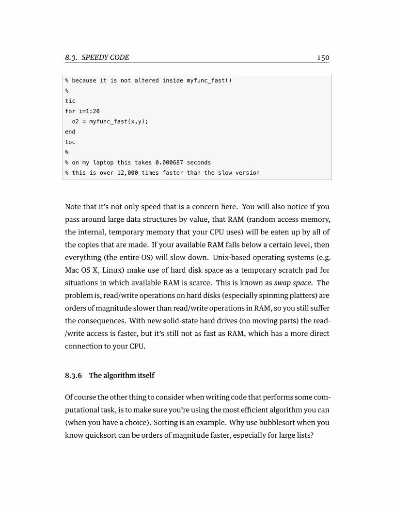
8.3. SPEEDY CODE 150
% because it is not altered inside myfunc_fast()
%
tic
for i=1:20
o2 = myfunc_fast(x,y);
end
toc
%
% on my laptop this takes 0.000687 seconds
% this is over 12,000 times faster than the slow version
Note that it’s not only speed that is a concern here. You will also notice if youpass around large data structures by value, that RAM (random access memory,the internal, temporary memory that your CPU uses) will be eaten up by all ofthe copies that are made. If your available RAM falls below a certain level, theneverything (the entire OS) will slow down. Unix-based operating systems (e.g.Mac OS X, Linux) make use of hard disk space as a temporary scratch pad forsituations in which available RAM is scarce. This is known as swap space. Theproblem is, read/write operations on hard disks (especially spinning platters) areorders ofmagnitude slower than read/write operations in RAM, so you still sufferthe consequences. With new solid-state hard drives (no moving parts) the read-/write access is faster, but it’s still not as fast as RAM, which has a more directconnection to your CPU.
8.3.6 The algorithm itself
Of course the other thing to considerwhenwriting code that performs some com-putational task, is to make sure you’re using the most efficient algorithm you can(when you have a choice). Sorting is an example. Why use bubblesort when youknow quicksort can be orders of magnitude faster, especially for large lists?

8.4. MATLAB CODER 151
Another example is optimization. For certain families of problems, specific op-timizers are known to be really fast and efficient. For others, one needs a moregeneric, more robust optimizer, that may be slower.
Whatver operation you’re coding up, do a bit of research to find out if someonehas developed an algorithm that solves the problem you’re solving, only faster.
8.4 MATLAB Coder
The MATLAB Coder is a toolbox which lets you generate standalone C and C++code from MATLAB code, and lets you generate binary MEX files which you cancall from your own MATLAB code.
Note that there is another MATLAB toolbox called the MATLAB Compiler, whichdoes something different—it lets you share MATLAB programs as standalone ap-plications. We will be talking about the MATLAB Coder here, not the MATLABCompiler.
Without getting into details (and there are a few, see the documentation) thewayto use the MATLAB Coder is to use the codegen function to generate a MEX filebased on some MATLAB function that you’ve written, and then to call that com-piled version of your function instead of the original MATLAB code version.
So for example let’s consider the following function which computes the stan-dard deviation of means of simulated random data vectors. It’s not so importantwhy we are doing these particular calculations—it’s just an example of a set ofcalculations that we can compile to make faster.
function out = myfunction(in)
out = zeros(1,in)*NaN;
for i=1:in
tmp = randn(100,5);
out(i) = std(mean(tmp));

8.4. MATLAB CODER 152
end
end
We can call the function like so:
>> tic; out=myfunction(1e5); toc
Elapsed time is 7.873669 seconds.
>> hist(out,50)
which produces the figure shown in Figure 8.7.
Figure 8.7: Output of myfunction.m.
To compile our MATLAB code into a binary MEX file we simply call the codegen
function:
>> codegen myfunction -args {double(0)}
The -args argument is a list of input parameters to our function myfunction and

8.4. MATLAB CODER 153
their types, which the MATLAB coder needs to know in advance, in order to pro-duce the C code and then the binary MEX function. The double(0) just tells MAT-LAB that we have a single input argument that is the same type as double(0), inother words a double.
Just to unpack this a bit more—if we had a function that took two input argu-ments, a scalar double and a 1x10 array of doubles then we could do the following:
>> i1 = 0.0;
>> i2 = zeros(1,10);
>> codegen myfunction -args {i1, i2}
In this case we have predefined example input variables and passed those on ina cell array (hence the curly brackets).
Now if we look in our current directory we will see a binary MEX file called my-
function_mex.mexmaci64:
>> !ls -l
total 136
drwxr-xr-x 3 plg staff 102 26 Aug 11:41 codegen
-rw-r--r--@ 1 plg staff 126 26 Aug 11:36 myfunction.m
-rwxr-xr-x 1 plg staff 62540 26 Aug 11:41 myfunction_mex.mexmaci64
We also see a directory called codegen that contains a subdirectory called mex andwithin that another directory called myfunction, that contains all of the various Cfiles and other stuff that’s required to build the binary MEX file:
>> !ls codegen/mex/myfunction
_coder_myfunction_api.o myfunction_initialize.c
_coder_myfunction_info.o myfunction_initialize.h
_coder_myfunction_mex.o myfunction_initialize.o
buildInfo.mat myfunction_mex.mexmaci64

8.4. MATLAB CODER 154
eml_error.c myfunction_mex.mk
eml_error.h myfunction_mex.mki
eml_error.o myfunction_mex.sh
html myfunction_mex_mex.map
interface myfunction_terminate.c
mean.c myfunction_terminate.h
mean.h myfunction_terminate.o
mean.o myfunction_types.h
myfunction.c randn.c
myfunction.h randn.h
myfunction.o randn.o
myfunction_data.c rt_nonfinite.h
myfunction_data.h rtwtypes.h
myfunction_data.o setEnv.sh
myfunction_emxutil.c std.c
myfunction_emxutil.h std.h
myfunction_emxutil.o std.o
So now to call our compiled version of the function we just call myfunction_mexinstead of calling myfunction:
>> tic; out=myfunction_mex(1e5); toc
Elapsed time is 0.981005 seconds.
>> hist(out,50)
We can see we already achieved a significant speedup, almost 10x.
The new MEX function produces the figure shown in Figure 8.8, which looks thesame as the one produced by the plain MATLAB code, so we have some notionthat our compiled MEX file is doing the right thing. Of course we should performmore stringent tests than this just to verifywe are getting the expectedbehaviourout of the binary MEX file.

8.4. MATLAB CODER 155
Figure 8.8: Output of myfunction_mex.
The MathWorks has a product page devoted to the Coder here:
MATLAB Coder product page95
The MathWorks also has a page on their online documentation devoted to theMATLAB Coder here:
MATLAB Coder online documentation96

LINKS 156
Links
93http://www.mathworks.com/help/matlab/debugging-code.html
94http://www.mathworks.com/help/matlab/matlab_prog/profiling-for-improving-performance.
html
95http://www.mathworks.com/products/matlab-coder
96http://www.mathworks.com/help/coder/index.html

9 Parallel programming
9.1 What is parallel computing?
Simply put, parallel computing refers to performing multiple computations inparallel, i.e. simultaneously. By default most operations that take place on yourcomputer happen in serial, that is, one at a time. These days CPU chips (eventhose on laptops) have multiple cores, which allow for some degree of paralleloperations.
In principle, every time you double the number of CPU cores (or CPUs them-selves), you can achieve something close to a halving of time to complete theoperations. In practice however, there is always some overhead cost in carryoutout the parallel computations. If the operations are at all lengthy however, theoverhead cost is always worth it.
There are several types of parallel computing, which we’ll talk briefly about (andwhich are listed below). What we’ll get hands-on experience with is symmetricmultiprocessing. This is the style of parallel computing where multiple CPUs, ormultiple cores on a single CPU, share access to the same memory (RAM) store,and can carry out operations in parallel.
Today (Fall, 2015), it’s still the case that not many programs take advantage ofmultiple cores. Operating systems, however, can take advantage of multiplecores through multithreading (see below), by assigning different threads to their
157

9.2. MULTI-THREADING 158
own processing nodes.
Some programs like MATLAB (and some Apple applications) come with the abil-ity to take advantage of multiple cores built-in. Due to the relative complexityof parallelizing serial code, however, most applications still operate in a serialfashion.
Parallel computing97 (Wikipedia)
9.2 Multi-threading
Modernoperating systems likeMacOSX, Linux, andotherUnixvariants, providethe ability for programs to spawnmultiple threads that execute independently ofeach other. The advantage of multithreading is that one process can do its workand other processes don’t have to wait until the working process is done. This isused extensively for graphical user interfaces.
When you copy a file, you can still move your mouse around, you can still startother programs, you can still browse the web, while other things are happeningsimultaneously. Multithreadingcanoccurona singleCPUwitha single core. Thisisn’t parallel computing per se, asmultiple threads still have to share a single CPUprocessing unit to do their work—but the operating systemmanages the multiplethreads so that the user has the impression that multiple things are happening atonce.
See the wikipedia article for more details:
Multithreading98 (wikipedia)
9.3 Symmetric Multiprocessing (SMP)
These days modern computers ship with CPUs that have multiple cores, or evenmultiple CPUs each with multiple cores. At the time of writing these notes (Fall

9.3. SYMMETRIC MULTIPROCESSING (SMP) 159
2015) you can for example buy a Mac Pro desktop computer with two 6-coreCPUs, for a total of 12 independent processing cores. With hyperthreading (seebelow) you get 24 processing cores, all for around $5,000—which seems like a lot,but just 10 years ago a computer cluster with 24 nodes would have cost around$75,000–$100,000.
When multiple CPUs and/or multiple CPU cores live in a single machine, theytypically all share access to the same physical RAM (memory). These days allApple desktops and laptopshaveCPUswithmultiple cores. Generic PCs also shipwith multiple CPUs and cores. Even smartphones (e.g. the iPhone, and Google’sNexus phone) come with multiple CPUs and multiple cores.
The great advantage of having multiple computing nodes in a single machine, isthat unlike multithreading on a single CPU, where the operating system has toswitch back and forth between each thread, with multiple CPUs/cores, each corecan execute a different task in parallel with the others (i.e. at the same time).
A good analogy is the following. Imagine someone gives me 10 decks of playingcards, and each deck has been shuffled, and my task is to re-order each deck ofcards. A computer with a single CPU/core is like a single person who is taskedwith sorting all 10 decks of cards. Iwould have to sort themall, one at a time, oneafter the other, i.e. in serial. I could implement “multithreading” by sorting onedeck for a few seconds, setting it aside, sorting the next deck for a few seconds,setting it aside, and soon, sorting bits of eachone, onebyone. It’s still happeningin serial though.
If I had access to other processing nodes, I could parallelize the task. So imagineinstead of me sorting all 10 decks, I found 9 other people to help me. I gave themone of the 10 decks of cards, and I took one. Now we can all sort them, at thesame time, in parallel. In theory it should take 1
10th the time compared to me
sorting them all myself, in serial. In fact though, there would be some overhead
9.4. HYPERTHREADING 160
cost, for example at the beginning, when I would have to hand out each deckand give everyone their instructions, and then at the end, when I would have tocollect all the sorted decks from each person. If the actual computational taskbeing parallelized is time intensive, however, then these overhead costs wouldbe minimal compared to the gain in speed I would achieve by parallelizing thetask.
Symmetric multiprocessing, i.e. having multiple independent processing unitsshare the same memory store, is advantageous compared to cluster or grid com-puting, where each processing node has its own memory. In the latter cases,there is a (sometimes relatively major) overhead cost involved in transferringdata to thememory store for each processing unit, and back again to a head node.When this transfer happens over a network, as you can imagine, this would beway slower than if it happens on a common logic board on which all processingcores sit (as is with the case of symmetric multiprocessing).
Here is a wikipedia article on symmetric multiprocessing:
Symmetric multiprocessing99 (wikipedia)
9.4 Hyperthreading
Hyperthreading is a proprietary implementation by Intel for allowing modernCPUs to behave as if they have twice asmany logical cores as physical cores. Thatis, if your CPU has two cores, hyperthreading implements a series of tricks at theoperating system level, that interface with a series of tricks at the hardware layer(i.e. in the CPU itself) that results in the ability to address four “logical” cores.
Unlike multithreading, which is simply a software implementation at the operat-ing system level, hyperthreading involves special implementations both at theoperating system level and at the hardware level. Current Apple laptops anddesktops all implement hyperthreading. Several generic PCs also implement hy-

9.5. CLUSTERS 161
perthreading.
For large, time consuming computations, hyperthreading won’t actually doublethe computation speed, since at the end of the day, there are still x physical cores,even though hyperthreading pretends there are 2x logical cores. If however eachcomputations is small, and doesn’t last a long time, hyperthreading can end upgiving you performance gains above and beyond regular multithreading, sinceit implements a number of efficiencies and tricks at the software and hardwarelayers.
For ourpurposes, hyperthreading is either there, or it isn’t, and it’s not somethingwe will be fiddling with. Here is a wikipedia article on hyperthreading:
Hyper-threading100 (wikipedia)
9.5 Clusters
So far we have been talking about a single machine with multiple CPUs and/ormultiple cores. Another way of implementing parallel computing is to connecttogether multiple machines, over a specialized local network. In principle onecan connect as many machines as one likes, to achieve just about any level ofparallelism one wants. Today’s fastest supercomputers101 are in fact clusters ofmachines hooked together. The world’s fastest supercomputer, as of today, Oc-tober 2015, is the Tianhe-2102, located in Guangzhou, China. It has 16,000 com-puter nodes, eachone comprising two Intel IvyBridgeXeonCPUs and threeXeonPhi chips for a total of 3,120,000 cores (3.12 million cores).
Sharcnet103 is a Canadian cluster computing facility with several individual clus-ters, the largest of which has 8,320 cores. Western has access to the Sharcnetclusters, you just have to sign up for an account.
Many individual researchers also operate smaller clusters, for example with 8, or

9.6. GRIDS 162
12, or 24 machines hooked together.
A relatively recent development is the advent of gigantic server farms oper-ated by private companies like Amazon and Google. Amazon’s Elastic ComputeCloud104 allows individuals to spawn multiple “virtual” machines, and hookthem together in networks and clusters, and run jobs on them. Cost is per ma-chine and per unit time, and so one can essentially (1) define your own clusterand (2) pay for only those minutes that you actually use. It’s a very flexible sys-tem that many researchers are beginning to utilize. Rhodri Cusack’s lab, for ex-ample, uses cloud-based machines for brain imaging data analysis.
The obvious advantage of a cluster over a single SMP machine, is that one canadd as many nodes onto the cluster (growing it as you go) to whatever size youwant (provided you can pay for it). The disadvantage is that data transfer overa network can be slower than a SMP machine where CPU cores share the sameRAM store. There is also added complexity in managing a cluster of machines,for example in configuring each one, and configuring a head node to manage allof the slave nodes. There is software out there that can organize this for you, forexampleOracleGrid Engine105, and others, but it’s still not trivial and takes someinvestment of time to fully implement.
Computer cluster106 (wikipedia)
9.6 Grids
Agrid is like a cluster, but the individualmachines are not on a local network, butthey can be anywhere on the internet. Sometimes multiple clusters are hookedtogether over the internet to form a grid. Sometimes a grid is composed of mul-tiple individual machines, spread out over multiple labs, multiple Departments,Univerisities, or even countries. Sometimes grids are set up so that individualmachines can be “taken over” as dedicated computational nodes. In other con-

9.7. GPU COMPUTING 163
figurations, individual machines only process grid jobs during their downtime,when for example the user is not using the machine for something else. One wayof setting this up is via a specialized screensaver. Wheneven the screensaver acti-vates (which is an indication that themachine is not beingused), the grid processstarts up and processes grid jobs.
Two classic examples of grids are the SETI@home107 grid (searching for extra-terrestrial life in the universe) and the Folding@home108 grid (simulations ofprotein folding for disease research). In each case, anyone around the world cansign up their machine to join the grid and donate computer time, install some lo-cal software, and then anytime their computer is not busy, it is recruited by thegrid to process data. As of now (Oct 2015) theFolding@homewebsite shows thatthere are 8,067,858 CPUs active right now on the Folding@home grid.
There are also nefarious uses for grids, which are sometimes called Botnet109s.In this case, a virus infects a user’s machine, installs a nefarious program, whichlies dormant until a central machine somewhere on the internet activates it, forsome nasty purpose (like a DDoS attack110, or for sending spam). Your machineessentially becomes a sleeper cell.
Grid computing111 (wikipedia)
9.7 GPU Computing
In recent years computer engineers and software developers have teamed up,and have delivered software libraries that allow developers to utilize graphicscards for more general purpose computing (GPGPU Computing).
Graphics cards, unlike CPUs, have hundreds if not thousands of cores, each ofwhich are typically used to process graphics for things like 3D games, video an-imation and scientific visualization. Each processing unit on a graphics cardis a much simpler beast than the cores on CPU chips—but for some computa-

9.8. TYPES OF PARALLEL PROBLEMS 164
tional tasks, one doesn’t need much complexity, and massive parallelism can beachieved by farming out general purpose computational tasks to the thousandsof cores on a graphics card.
For example, today (Oct 2015) for around $5,000 one can purchase an NVidiaTeslaGPU112,which is a singlegraphics card, thathas12GBofGPUmemory, 2880cores, and has a processing power of 1.43 Tflops. As you can imagine, if yourcomputational task is well suited to GPU processing, running it on 2880 coreswill be quite a bit faster than running on 4, 8 or 12 cores (e.g. that you get with amodern dual 6-core CPU Mac Pro).
There are two major C/C++ software libraries that provide relatively high-levelinterfaces to performing general purpose computation on graphics cards
• CUDA113 (Nvidia proprietary)• OpenCL114 (open)
MATLAB’s Parallel Computing Toolbox has the ability to farm out some compu-tations to NVidia CUDA-enabled GPUs, see this page for more info:
MATLAB GPU Computing Support for NVIDIA CUDA-Enabled GPUs115
See this wikipedia page for more general information on GPGPU Computing:
GPGPU Computing116
9.8 Types of Parallel problems
Multithreading is an example of fine-grained parallelism (many shared opera-tions per second), in which the operating system manages (e.g. switches be-tween) threads at a very fast rate, e.g. with each CPU clock cycle. This can thushappen many times per second. This is what your operating system does in thebackground, as you are interactingwith your graphical user interface, surfing theweb, playing music, processing video in the background, all the while copying

9.9. MATLAB 165
files from one disk to another.
In another kind of fine-grained parallelism, multiple processes communicatewith each other many, many times per second.
In coarse-grained parallelism, there are many, many independent threads/tasks,that rarely or never communicate with each other.
Finally, so-called embarassingly parallel problems are 100% independent opera-tions, and never communicate with each other. Each process doesn’t depend inany way on the result of another operation. This is the kind of parallelism thatwe will be talking about in this class.
9.9 MATLAB
MATLAB provides parallel computing via its Parallel Computing Toolbox (see be-low).
• MATLAB Parallel Computing Toolbox117
• MATLAB Execute loop iterations in parallel using parfor118
• MATLAB Getting Started with parfor119
• MATLAB Parallel Computing Toolbox Examples120
9.10 Shell scripts
Finally, one canparallelize tasks at the level of the shell, even if the programsyouwrite/run aren’t parallelized, using a tool like GNU Parallel (see below). Briefly,with GNU Parallel you can split a list of (ambarassingly parallel) tasks across mul-tiple cores even if the program itself is serial in nature. See the GNU Parallel pagebelow and the tutorial page for some examples. In our lab we use GNU Parallelto distribute subject-level brain imaging processing across multiple cores.
• GNU Parallel121

9.10. SHELL SCRIPTS 166
• GNU Parallel tutorial122
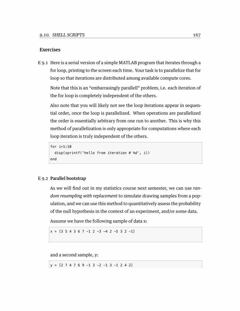
9.10. SHELL SCRIPTS 167
Exercises
E 9.1 Here is a serial version of a simple MATLAB program that iterates through afor loop, printing to the screen each time. Your task is to parallelize that forloop so that iterations are distributed among available compute cores.
Note that this is an “embarrasingly parallell” problem, i.e. each iteration ofthe for loop is completely independent of the others.
Also note that you will likely not see the loop iterations appear in sequen-tial order, once the loop is parallelized. When operations are parallelizedthe order is essentially arbitrary from one run to another. This is why thismethod of parallelization is only appropriate for computations where eachloop iteration is truly independent of the others.
for i=1:10
disp(sprintf('hello from iteration # %d', i))
end
E 9.2 Parallel bootstrap
As we will find out in my statistics course next semester, we can use ran-dom resampling with replacement to simulate drawing samples from a pop-ulation, and we can use this method to quantitatively assess the probabilityof the null hypothesis in the context of an experiment, and/or some data.
Assume we have the following sample of data x:
x = [3 5 4 3 6 7 -1 2 -3 -4 2 -5 3 2 -1]
and a second sample, y:
y = [2 7 4 7 6 9 -1 3 -2 -1 3 -1 2 4 2]

9.10. SHELL SCRIPTS 168
The mean of the sample x is 1.533 and the mean of sample y is 2.933. Let’scompute a statistic we’ll call dsamp which is the difference between means,y− xwhich in this case is equal to dsamp = 1.400.
The null hypothesis is that the sampleswere taken froma single populationwith the same mean, and so dpop = 0.00, and any departure from this in oursample statistic dsamp is due to random sampling error.
Question 1
Use bootstrapping to compute the probability of the null hypothesis, withone million bootstrap (re)samples. Write your code in the usual serial fash-ion, using for-loop(s).
Question 2
Rewrite your solution to question 1, and parallelize the bootstrap. In otherwords execute theonemillionbootstrap iterations inparallel,with theworkspread over your available compute cores.

LINKS 169
Links
97http://en.wikipedia.org/wiki/Parallel_computing
98http://en.wikipedia.org/wiki/Multithreading_(computer_architecture)
99http://en.wikipedia.org/wiki/Symmetric_multiprocessing
100http://en.wikipedia.org/wiki/Hyper-threading
101http://en.wikipedia.org/wiki/Supercomputer
102http://en.wikipedia.org/wiki/Tianhe-2
103https://www.sharcnet.ca/my/front/
104http://aws.amazon.com/ec2/
105http://en.wikipedia.org/wiki/Oracle_Grid_Engine
106http://en.wikipedia.org/wiki/Cluster_(computing)
107http://en.wikipedia.org/wiki/SETI@Home
108http://en.wikipedia.org/wiki/Folding@home
109http://en.wikipedia.org/wiki/Botnet
110http://en.wikipedia.org/wiki/Distributed_denial-of-service_attack#Distributed_
attack
111http://en.wikipedia.org/wiki/Grid_computing
112http://www.nvidia.com/object/tesla-workstations.html
113http://www.nvidia.com/object/cuda_home_new.html
114http://www.khronos.org/opencl/
115http://www.mathworks.com/discovery/matlab-gpu.html
116http://en.wikipedia.org/wiki/General-purpose_computing_on_graphics_processing_
units
117http://www.mathworks.com/products/parallel-computing/
118http://www.mathworks.com/help/distcomp/parfor.html

LINKS 170
119http://www.mathworks.com/help/distcomp/getting-started-with-parfor.html
120http://www.mathworks.com/help/distcomp/examples/
121http://www.gnu.org/software/parallel/
122http://www.gnu.org/software/parallel/parallel_tutorial.html

10 Graphical displays of data
MATLAB comes with lots of built-in functionality for generating both 2-D and3-D graphics. You will learn a collection of commands (mainly plot()) that willenable you do generate plots and configure their appearance with just about anydegree of precision you want. The great advantage of generating graphics purelybasedon scripted commands (as opposed for example to graphical, pointy-clickyapproaches based on graphical user interfaces (GUIs)) is that you can easily andinstantly re-generate graphics simply by re-running the script(s). In additionmaking changes to your graphics becomes a simple matter of tweaking com-mands and scripts.
Rather than writing notes that essentially duplicate the extensive online docu-mentation includedwithMATLAB, Iwill instead point you to some intial startinglocations where you can learn about generating graphics in MATLAB.
Graphics in MATLAB123
CommonGraphicsFunctions inMATLAB124 (a graphicalmenu showingdifferentkinds of plots and how to generate them)
2-D and 3-D Plots125
The plot() command126
Creating 2-D Graphs and Customizing Lines127
Add Titles, Axis Labels and Legends to Graphs128
171

172
Figures with multiple axes using subplots129
3-D Surface and Mesh Plots130
Shaded Polygons131
Customizing graphics by setting properties of the underlying objects132

173
Exercises
E 10.1 Line Plot
Let x be a vector:
[0,0.1,0.2,0.3,0.4,0.5,0.6,0.7,0.8,0.9]
and set y to be equal to sin(2*pi*x).
Generate a line plot that looks like this:
Smoother Line
Redefine x and y to make the curve smoother:

174
Change Line Colour
Plot it again but make the line blue, and thick:
E 10.2 Bar Plot
Let y be a vector with the following values:
[10, 8, 6, 4, 6, 8, 6, 2]

175
Generate the following bar plot:
Again with x labels
Plot it again but this time include labels on the x axis:
E 10.3 Multiline plot
Let x, y1, y2, and y3 be vectors:

176
x = [1,2,3,4,5]
y1 = [1,2,3,4,4]
y2 = [1,5,6,8,10]
y3 = [5,4,2,2,1]
Generate a multi-line plot like this:
Add a Legend
Add a legend to your plot that looks like this:
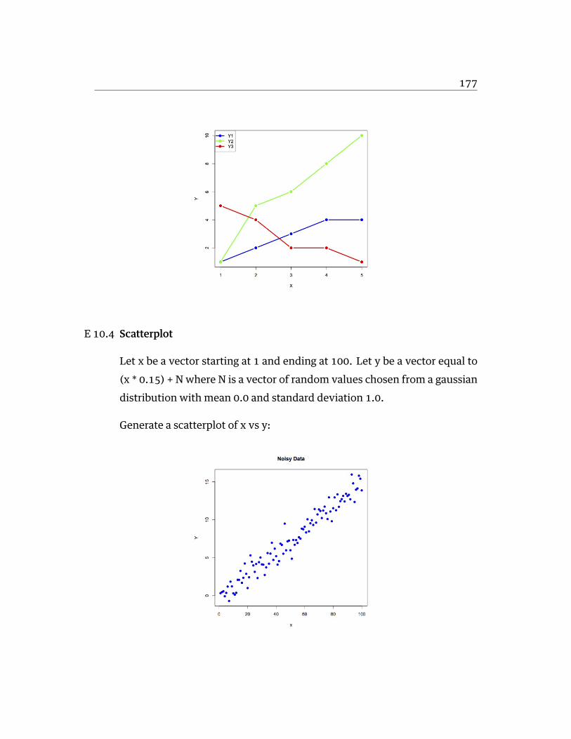
177
E 10.4 Scatterplot
Let x be a vector starting at 1 and ending at 100. Let y be a vector equal to(x * 0.15) + N where N is a vector of random values chosen from a gaussiandistribution with mean 0.0 and standard deviation 1.0.
Generate a scatterplot of x vs y:

178
A second variable
Let z be equal to ((x * 0.05) + 2) + N where N is a vector of random valueschosen from a gaussian distribution with mean 0.0 and standard deviation1.5.
Generate a scatterplot of y and z vs x, including a legend:
E 10.5 Subplots
Let x be a vector starting at 1 and ending at 100. Let y be a vector equal to(x * 0.15) + N where N is a vector of random values chosen from a gaussiandistribution with mean 0.0 and standard deviation 1.0.
Let z be equal to ((x * 0.05) + 2) + N where N is a vector of random valueschosen from a gaussian distribution with mean 0.0 and standard deviation1.5.
Generate a figure with scatterplots of (x vs y) and (x vs z) in separate sub-plots, stacked vertically:
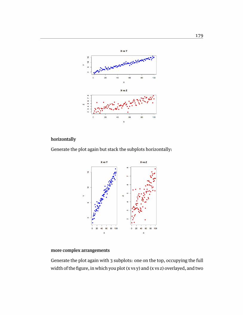
179
horizontally
Generate the plot again but stack the subplots horizontally:
more complex arrangements
Generate the plot again with 3 subplots: one on the top, occupying the fullwidthof thefigure, inwhichyouplot (x vs y) and (xvs z) overlayed, and two

180
on the bottom, in which you plot (x vs y) in one and (x vs z) in the other:
E 10.6 Histograms
Define a variable y that contains 1000 values drawn from a gaussian dis-tribution with mean 0.0 and standard deviation 1.0. Plot a histogram of y.For now just use the default settings for whatever function you find thatproduces a histogram.

181
Number of bins
Replot the histogram using 25 bins:
Bin width
Replot the histogram using a bin width of 0.20:
E 10.7 Line of best fit

182
Let x be a vector starting at 1 and ending at 100. Let y be a vector equal to(x * 0.15) + N where N is a vector of random values chosen from a gaussiandistribution with mean 0.0 and standard deviation 1.0.
Generate a scatterplot of (x vs y) and overlay on the plot, the line of best fitafter fitting a linear model to the data: y = β0 + β1x.
Add a legend

183
Add the equation of the line
E 10.8 Surface plot
Define x and y each over a grid [-8,8] in steps of 0.5.
Define r =√x2 + y2 + 0.00001.
Define z = sin(r)/r
Generate the following surface plot:

LINKS 184
Links
123http://www.mathworks.com/help/matlab/graphics.html
124http://www.mathworks.com/help/matlab/creating_plots/types-of-matlab-plots.
html#btjs9s4-1
125http://www.mathworks.com/help/matlab/2-and-3d-plots.html
126http://www.mathworks.com/help/matlab/ref/plot.html
127http://www.mathworks.com/help/matlab/creating_plots/using-high-level-plotting-functions.
html
128http://www.mathworks.com/help/matlab/creating_plots/add-title-axis-labels-and-legend-to-graph.
html
129http://www.mathworks.com/help/matlab/creating_plots/create-graph-with-subplots.
html
130http://www.mathworks.com/help/matlab/surface-and-mesh-plots-1.html
131http://www.mathworks.com/help/matlab/geometry.html
132http://www.mathworks.com/help/matlab/graphics-objects.html
11 Signals, sampling & filtering
Whereas signals in nature (such as sound waves, magnetic fields, hand posi-tion, electromyograms (EMG), electroencephalograms (EEG), extra-cellular po-tentials, etc) vary continuously, often in science we measure these signals bysampling them repeatedly over time, at some sampling frequency. The resultingcollection of measurements is a discretized representation of the original contin-uous signal.
Beforeweget into sampling theoryhoweverweshouldfirst talk abouthowsignalscan be represented both in the time domain and in the frequency domain.
Jack Schaedler has a nice page explaining and visualizing many concepts dis-cussed in this chapter:
Seeing circles, sines and signals133
11.1 Time domain representation of signals
This is how you are probably used to thinking about signals, namely how themagnitude of a signal varies over time. So for example a signal s containing asinusoid with a period T of 0.5 seconds (a frequency of 2 Hz) and a peak-to-peakmagnitude b of 2 volts is represented in the time domain t as:
s(t) =(b2
)sin (wt) (11.1)
185

11.2. FREQUENCY DOMAIN REPRESENTATION OF SIGNALS 186
where
w =2πT (11.2)
We can visualize the signal by plotting its magnitude as a function of time, asshown in Figure 11.1.
Figure 11.1: Time domain representation of a signal.
11.2 Frequency domain representation of signals
Wecanalso represent signals in the frequencydomain. This requires someunder-standing of the Fourier series134. The idea of the Fourier series is that all periodicsignals can be represented by (decomposed into) the sum of a set of pure sinesand cosines that differ in frequency and period. See the wikipedia link for lots ofdetails and a helpful animation.
s(t) = a02 +
∞∑n=1
[ancos(nwt) + bnsin(nwt)] (11.3)
The coefficients an and bn define the weighting of the different sines and cosinesat different frequencies. In other words these coefficients represent the strength

11.3. FAST FOURIER TRANSFORM (FFT) 187
of the different frequency components in the signal.
We can also represent the Fourier series using only sines:
s(t) = a02
∞∑n=1
[rncos(nwt− φn)]
(11.4)
Using this formulation we now have magnitude coefficients rn and phase coef-ficients φn. That is, we are representing the original signal s(t) using a sum ofsinusoids of different frequencies and phases.
Here is a web page that lets you play with how sines and cosines can be used torepresent different signals: Fourier series visualization135.
11.3 Fast Fourier transform (FFT)
Given a signal there is a very efficient computational algorithm called the FastFourier transform136 (FFT) for computing the magnitude and phase coefficients.We will not go into the details of this algorithm here, most high level program-ming languages have a library that includes the FFT algorithm.
Here is a video showing a 100-year-old mechanical computer that does both for-ward and inverse Fourier transforms:
• Harmonic Analyzer (1/4)137
• Harmonic Analyzer (2/4)138
• Harmonic Analyzer (3/4)139
• Harmonic Analyzer (4/4)140
11.4 Sampling
Before we talk about the FFT and magnitude and phase coefficients, we need totalk about discrete versus continuous signals, and sampling. In theory we can

11.4. SAMPLING 188
derive a mathematical description of the Fourier decomposition of a continuoussignal, as we have done above, in terms of an infinite number of sinusoids. Inpractice however, signals are not continuous, but are sampled at some discretesampling rate.
For example, when we use Optotrak to record the position of the fingertip dur-ing pointing experiments, we choose a sampling rate of 200 Hz. This means 200times per second the measurement instrument samples and records the positionof the fingertip. The interval between any two samples is 5 ms. It turns out thatthe sampling rate used has a specific effect on the number of frequencies used ina discrete Fourier representation of the recorded signals.
The Shannon-Nyquist sampling theorem141 states that a signal must be sampledat a rate which is at least twice that of its highest frequency component. If a sig-nal contains power at frequencies higher than half the sampling rate, these highfrequency components will appear in the sampled data at lower frequencies andwill distort the recording. This is known as the problem of aliasing142.
Let’s look at a concrete example that will illustrate this concept. Let’s assume wehave a signal thatwewant to sample, andwe choose a sampling rate of 4Hz. Thismeans every 250 ms we sample the signal. According to the Shannon-Nyquisttheorem, the maximum frequency we can uniquely identify is half that, whichis 2 Hz. This is called the nyquist frequency143. Let’s look at a plot and see whythis is so.
In Figure 11.2 we see a solid blue line showing a 2 Hz signal, a magenta dashedline showing a 4 Hz signal, and a green dashed line showing a 8 Hz signal. Nowimagine we sample these signals at 2 Hz, indicated by the vertical red lines. No-tice that at the sample points (vertical red lines), the 2 Hz, 4 Hz and 8 Hz sig-nals overlap with identical values. This means that on the basis of our 2 Hzsamples, we cannot distinguish between frequencies of 2, 4 and 8 Hz. What’s

11.4. SAMPLING 189
more, what this means is that if the signal we are actually sampling at 2 Hz hassignificant signal power at frequencies above the Nyquist (1 Hz) then the powerat these higher frequencies will influence our estimates of the magnitude coef-ficients corresponding to frequencies below the Nyquist... in other words thehigh-frequency power will be aliased into the lower frequency estimates.
Figure 11.2: Signal aliasing.
Figure 11.3 shows another example taken from the wikipedia article on alias-ing144. Here we have two sinusoids—one at 0.1 Hz (blue) and another at 0.9 Hz(red). We sample both at a sampling rate of 1 Hz (vertical green lines). You cansee that at the sample points, both the 0.1 Hz and 0.9 Hz sinusoids pass throughthe sample points and thus both would influence our estimates of the power atthe 0.1 Hz frequency. Since the sampling rate is 1 Hz, the Nyquist frequency (themaximum frequency we can distinguish) is 0.5 Hz—and so any power in the sig-nal above 0.5 Hz (such as 0.9 Hz) will be aliased down into the lower frequencies(in this case into the 0.1 Hz band).
Figure 11.3: Signal aliasing sinusoids.
So the message here is that in advance, before choosing your sampling rate, you

11.5. POWER SPECTRA 190
should have some knowledge about the highest frequency that you (a) are in-terested in identifying; and (b) you think is a real component in the signal (asopposed to random noise). In cases where you have no a priori knowledge aboutthe expected frequency content, one strategy is to remove high frequency com-ponents before sampling. This can be accomplished using low-pass filtering—sometimes called anti-aliasing filters. Once the signal has been sampled, it’s toolate to perform anti-aliasing.
11.5 Power spectra
Having bypassed completely the computational details of how magnitude andphase coefficients are estimated, we will now talk about how to interpret them.
For a given signal, the collection of magnitude coefficients gives a description ofthe signal in terms of the strength of the various underlying frequency compo-nents. For our immediate purposes these magnitude coefficients will be mostimportant to us and we can for the moment set aside the phase coefficients.
Here is an example of a power spectrum for a pure 10 Hz signal, sampled at 100Hz.
Figure 11.4: Power spectrum for a pure 10 Hz signal.
The magnitude values are zero for every frequency except 10 Hz. We haven’t

11.5. POWER SPECTRA 191
plotted the phase coefficients. The set of magnitude and phase coefficients de-rived from a Fourier analysis is a complete description of the underlying signal,with one caveat—only frequencies up to the Nyquist are represented. So the ideahere is that one can go between the original time-domain representation of thesignal and this frequency domain representation of the signal without losing in-formation. As we shall see below in the section on filtering, we can perform oper-ations in the frequency domain and then transform back into the time domain.
Here is some MATLAB code to illustrate these concepts. We construct a one sec-ond signal sampled at 100 Hz that is composed of a 6 Hz, 10 Hz and 13 Hz com-ponent. We then use the fft() function to compute the Fast Fourier transform,we extract the magnitude information, we set our frequency range (up to theNyquist) and we plot the spectrum, which is shown in Figure 11.5.
t = linspace(0,1,100);
y = sin(2*pi*t*6) + sin(2*pi*t*10) + sin(2*pi*t*13);
figure;
subplot(2,1,1)
plot(t,y)
xlabel('Time (sec)')
ylabel('Signal Amplitude')
subplot(2,1,2)
out = fft(y);
mag = abs(real(out));
plot(0:49, mag(1:50));
set(gca,'xlim',[0 50]);
xlabel('Frequency Component (Hz)')
ylabel('Amplitude')
Wecan see that thepower spectrumhas revealedpeaks at 6, 10 and13Hz—whichwe know is correct, since we designed our signal from scratch.
Typically however signals in the real world that we record are not pure sinusoids,

11.6. POWER SPECTRAL DENSITY 192
Figure 11.5: A signal with 6, 10 and 13 Hz pure sinusoids, and its spectrum.
but contain random noise. Noise can originate from the actual underlying pro-cess that we are interested in measuring, and it can also originate from the in-struments we use to measure the signal. For noisy signals, the FFT taken acrossthe whole signal can be noisy as well, and can make it difficult to see peaks.
11.6 Power Spectral Density
One solution is instead of performing the FFT on the entire signal all at once, toinstead, split the signal into chunks, take the FFT of each chunk, and then av-erage these spectra to come up with a smoother spectrum. This can be accom-plished using a power spectral density145 function. In MATLAB there is a func-tion pwelch() to accomplish this. We won’t go into the mathematical details orthe theoretical considerations (relating to stochastic processes) but for now suf-fice it to say that the psd can often give you a better estimate of the power atdifferent frequencies compared to a “plain” FFT.
Here is an example of plotting the power spectral density of a signal in MATLAB.We construct a 50 Hz signal at 1000 Hz sampling rate, and we add some randomnoise on top:

11.6. POWER SPECTRAL DENSITY 193
t = linspace(0,1,1000);
y = sin(2*pi*t*50);
yn = y + randn(size(y))*1;
figure
subplot(3,1,1)
plot(t,yn)
xlabel('Time (sec)')
ylabel('Signal Amplitude')
title('TIME SERIES SIGNAL')
subplot(3,1,2)
out = fft(yn);
mag = abs(real(out));
plot(0:499,mag(1:500));
xlabel('Frequency (Hz)')
set(gca,'xlim',[0 100])
ylabel('Power')
title('RAW FFT')
subplot(3,1,3)
pwelch(yn,[],[],[],1000);
set(gca,'xlim',[0 100])
xlabel('Frequency (Hz)')
ylabel('PSD')
title('PSD')
In Figure 11.6 you can see that the peak at 50Hz stands nicely above all the noisein the power spectral density estimate (bottom panel), while int the raw FFT it’sdifficult to see the 50 Hz peak against the noise (middle panel).
We have been ignoring the phase of the signal here, but just like the magnitudecoefficients over frequencies, we can recover the phase coefficients of the signalas well.

11.7. DECIBEL SCALE 194
Figure 11.6: Power spectral density of a 50 Hz signal.
11.7 Decibel scale
The decibel (dB) scale is a ratio scale. It is commonly used to measure soundlevel but is also widely used in electronics and signal processing. The dB is a log-arithmic unit used to describe a ratio. You will often see power spectra displayedin units of decibels.
The difference between two sound levels (or two power levels, as in the case ofthe power spectra above), is defined to be:

11.8. SPECTROGRAM 195
20(log10)P2P1
dB (11.5)
Thus when P2 is twice as large as P1, then the difference is about 6 dB. When P2is 10 times as large as P1, the difference is 20 dB. A 100 times difference is 40 dB.
An advantage of using the dB scale is that it is easier to see small signal compo-nents in the presence of large ones. In other words large components don’t visu-ally swamp small ones.
Since the dB scale is a ratio scale, to compute absolute levels one needs areference—a zero point. In acoustics this reference is usually 20 micropascals—about the limit of sensitivity of the human ear.
For our purposes in the absence of a meaningful reference we can use 1.0 as thereference (i.e. as P1 in the above equation).
11.8 Spectrogram
Often there are times when you may want to examine how the power spectrumof a signal (in other words its frequency content) changes over time. In speechacoustics for example, at certain frequencies, bands of energy called formants146
may be identified, and are associated with certain speech sounds like vowels andvowel transitions. It is thought that the neural systems for human speech recog-nition are tuned for identification of these formants.
Essentially a spectrogram is away tovisualize a series ofpower spectra computedfrom slices of a signal over time. Imagine a series of single power spectra (fre-quency versus power) repeated over time and stacked next to each other over atime axis.
MATLAB has a built-in function called spectrogram() that will generate a spectro-gram. MATLAB has a sample audio file called mtlb.matwhich can be loaded from

11.9. FILTERING 196
the command line:
load mtlb
spectrogram(mtlb,256,230,256,Fs,'yaxis')
sound(mtlb)
Figure 11.7 shows the resulting spectrogram. Time is on the horizontal axis andfrequency is on the vertical axis. The colours indicate the power of the differentfrequencies at the given time points.
Figure 11.7: Spectrogram of the sound “MATLAB”.
11.9 Filtering
The Fourier series representation and its computational implementation, theFFT and the PSD, are useful not only for determining what frequency com- po-nents are present in a signal, but we can also perform operations within fre-quency space in order to manipulate the strength of different frequency compo-nents in the signal. This can be especially effective for eliminating noise sourceswith known frequency content.
Let’s look at a concrete example:

11.9. FILTERING 197
t = linspace(0,1,1000);
y = sin(2*pi*t*6) + sin(2*pi*t*10) + sin(2*pi*t*13);
yn = y + randn(size(y))*0.5;
[x,y,f] = fft_plus(yn,1000);
semilogx(f,20*log10(x));
xlabel('Frequency (Hz)')
ylabel('Power (dB)')
Figure 11.8: A spectrum of a noisy signal with peaks at 6, 10 and 13 Hz.
In Figure 11.8 we can see the signal has three signal components: 6, 10 and 13Hz. Let’s say we believe that the frequencies we are interested in are all below20 Hz. In other words, frequencies above that are assumed to be noise of onesort or another. We can filter the signal so that all frequencies above 20 Hz areessentially zeroed out (or at least reduced in magnitude). One way to do this issimply to take the vector of power coefficients, change all values for frequenciesabove 20Hz to zero, and performan inverse Fourier transform (the inverse of theFFT) to go back to the time domain. We won’t go into the mathematical details,but there are also other ways to filter a signal as well.
Here is a short summary of different kinds of filters, and some terminology.

11.9. FILTERING 198
• low-pass filters pass low frequencies without change, but attenuate (i.e. re-duce) frequencies above the cutoff frequency
• high-pass filterspass high frequencies and attenuate low frequencies, belowthe cutoff frequency
•• band-pass filters pass frequencies within a pass band frequency range and
attenuate all others• band-stop filters (sometimes called band-reject filters or notch filters) atten-
uate frequencies within the stop band and pass all others
In the code example aboveweuse a function called fft_plus, which convenientlyperforms the FFT and converts the results into a format that is useful. Here is thefunction:
function [x, y, f] = fft_plus (xin, rate, winsize)
%
% function [x, y, f] = fft_plus (xin, rate, winsize)
% fft computations - normalized to give 'single-sided' results
%
% inputs: xin = signal, rate = sampling rate (Hz)
% winsize (optional) window size for computing FFT
% outputs: x = magnitude, y = phase, f = frequency
%
if nargin==2
winsize = length(xin);
end;
fx = fft(xin,winsize);
N=length(fx);
fx(2:N) = fx(2:N)*(2/N);
fx(1)=fx(1)/N;

11.9. FILTERING 199
x=abs(fx);
y=angle(fx); % radians
f=(0:N-1)/N;
f=f*rate;
nq = floor(N/2);
x=x(1:nq);
y=y(1:nq);
f=f(1:nq);
end
You might also be interested in a function called fft_plot, which generates a nicelooking plot of magnitude and phase againt frequency (it calls fft_plus to do itswork). Here is the code:
function fft_plot(xin, rate, logaxis, winsize)
%
% function dum = fft_plot(xin, rate, winsize)
% generates a plot of magnitude and phase against frequency
%
% inputs: xin = signal, rate = sampling rate (Hz)
% winsize (optional) window size for computing FFT
% outputs: none
%
if nargin==2
logaxis = 1;
end
[X,Y,F] = fft_plus(xin,rate);
subplot(2,1,1)

11.9. FILTERING 200
if logaxis==1
semilogx(F, 20.*log10(X))
else
plot(F, 20.*log10(X))
end
grid on
xlabel('Frequency (Hz)')
ylabel('Magnitude (dB)')
drawnow
subplot(2,1,2)
if logaxis==1
semilogx(F, unwrap(Y))
else
plot(F, unwrap(Y))
end
grid on
xlabel('Frequency (Hz)')
ylabel('Phase (deg)')
drawnow
end
11.9.1 Characterizing filter performance
A useful way of characterizing a filter’s performance is in terms of the ratio of theamplitude of the output to the input (the amplitude ratio AR or gain), and thephase shift (φ) between the input and output, as functions of frequency. A plotof the amplitude ratio and phase shift against frequency is called a Bode plot147.
The pass band of a filter is the range of frequencies over which signals pass withno change. The stop band refers to the range of frequencies over which a filterattenuates signals. The cutoff frequency or corner frequency of a filter is used todescribe the transition point from the pass band to the reject band. This this

11.9. FILTERING 201
transition cannot occur instantaneously it is usually defined to be the point atwhich the filter output is equal to -6 dB of the input in the pass band. The cutofffrequency is sometimes called the -6 dB point or the half-power point since -6dB corresponds to half the signal power. The roll-off refers to the rate at whichthe filter attenuates the input after the cutoff point. When the roll-off is linear itcan be specified as a specific slope, e.g. in terms of dB/decade or dB/octave (anoctave is a doubling in frequency).
Let’s look at some examples of filter characteristics.
Figure 11.9: Spectrum of three filtered versions of a noisy signal with peaks at 6, 10 and13 Hz.
In Figure 11.9 the blue trace shows the power spectrum for the unfiltered sig-nal. The red trace shows a lowpass-filtered version of the signal with a cutofffrequency of 30 Hz. The green trace shows a low-pass with a cutoff frequency of130 Hz. Also notice that the roll-off of the 30 Hz lowpass is not as great as for the130 Hz lowpass, which has a higher roll-off.
Here is a function in MATLAB to perform low-pass filtering:
function newdata = lowpass(data,samprate,cutoff,order)

11.9. FILTERING 202
% newdata = lowpass(data,samprate,cutoff,order)
%
% performs a lowpass filtering of the input data
% using an nth order zero phase lag butterworth filter
if nargin==3 order=2; end; % default to 2nd order
% get filter paramters A and B
[B,A] = butter(order,cutoff/(samprate/2));
% perform filtering
newdata = filtfilt(B,A,data);
Here is one to perform high-pass filtering:
function newdata = highpass(data,samprate,cutoff,order)
% newdata = highpass(data,samprate,cutoff,order)
%
% performs a highpass filtering of the input data
% using an nth order zero phase lag butterworth filter
if nargin==3 order=2; end;
[B,A] = butter(order,cutoff/(samprate/2),'high');
newdata = filtfilt(B,A,data);
Here is one for band-pass filtering:
function newdata = bandpass(data,samprate,cutoff,order)
% newdata = bandpass(data,samprate,cutoff,order)
%

11.9. FILTERING 203
% performs a bandpass filtering of the input data
% using an nth order zero phase lag butterworth filter
if nargin==3 order=2; end;
[B,A] = butter(order/2,cutoff./(samprate/2));
newdata = filtfilt(B,A,data);
Here is one for band-stop filtering:
function newdata = bandstop(data,samprate,cutoff,order)
% newdata = bandstop(data,samprate,cutoff,order)
%
% performs a bandstop filtering of the input data
% using an nth order zero phase lag butterworth filter
if nargin==3 order=2; end;
[B,A] = butter(order/2,cutoff./(samprate/2),'stop');
newdata = filtfilt(B,A,data);
Figure 11.10 shows the corresponding signals shown in the time-domain:
In the code we use a two-pass, bi-directional filter function (called filtfilt())to apply the butterworth filter to the signal. One-way single-pass filter functions(e.g. filter()) introduce time lags. This iswhy in real-time applications inwhichyou want to filter signals in real time (e.g. to reduce noise) there are time lagsintroduced.
So we see a very good example of how low-pass filtering can be used very ef-

11.9. FILTERING 204
fectively to filter out random noise. Key is the appropriate choice of cut-off fre-quency.
11.9.2 Common Filters
There are many different designs of filters, each with their own characteristics(gain, phase and delay characteristics). Some common types:
• Butterworth Filters have frequency responses which are maximally flat andhave a monotonic roll-off. They are well behaved and this makes them verypopular choices for simple filtering applications. For example in my work Iuse them exlusively for filtering physiological signals. MATLAB has a built-in function called butter() that implements the butterworth filter.
• Tschebyschev Filters provide a steeper monotonic roll-off, but at the ex-pense of some ripple (oscillatory noise) in the pass-band.
• Cauer Filters provide a sharper roll-off still, but at the expense of ripple inboth the pass-band and the stop-band, and reduced stop-band attenuation.
• Bessel Filters have a phase-shift which is linear with frequency in the pass-band. This corresponds to a pure delay and so Bessel filters preserve theshape of the signal quitewell. The roll-off ismonotonic and approaches thesame slope as the Butterworth and Tschebyschev filters at high frequenciesalthough it has a more gentle roll-off near the corner frequency.
11.9.3 Filter order
In filter design148 the order of a filter is one characteristic that you might comeacross. Technically the definition of the filter order is the highest exponent inthe z-domain149 (transfer function150) of a digital filter151. That’s helpful isn’t it!(not) Another way of describing filter order is the degree of the approximatingpolynomial for the filter. Yet another way of describing it is that increasing thefilter order increases roll-off and brings the filter closer to the ideal response (i.e.

11.9. FILTERING 205
a “brick wall” roll-off).
Practically speaking, youwill find that a second-order butterworthfilter providesa nice sharp roll-off without too much undesirable side-effects (e.g. large timelag, ripple in the pass-band, etc).
See this section152 of the wikipedia page on low-pass filters for another descrip-tion.
11.9.4 High-frequency noise and taking derivatives
Oneof the characteristics of just about anyexperimentalmeasurement is that thesignal that you measure with your instrument will contain a combination of truesignal and “noise” (random variations in the signal). A common approach is totake many measurements and average them together. This is what is commonlydone in EEG/ERP studies, in EMG studies, with spike-triggered averaging, andmany others. The idea is that if the “real” part of the signal is constant over trials,and the “noise”part of the signal is randomfrom trial to trial, then averagingovermany trials will average out the noise (which is sometimes positive, sometimesnegative, but on balance, zero) and what remains will be the true signal.
You can imagine however that there are downsides to this approach. First of all,it requires thatmany, manymeasures be taken so that averages can be computed.Second, there is noguarantee that theunderlying “true” signalwill in fact remainconstant over those many measurements. Third, one cannot easily do analyseson single trials, since we have to wait for the average before we can look at thedata.
One solution is to use signal processing techniques such as filtering to separatethe noise from the signal. A limitation of this technique however is thatwhen weapply a filter (for example a low-pass filter), we filter out all power in the signalabove the cutoff frequency—whether “real” signal or noise. This approach thus

11.9. FILTERING 206
assumes thatwe are fairly certain that the power above our cutoff is of no interestto us.
One salient reason to low-pass filter a signal, and remove high-frequency noise,is for cases inwhichweare interested in taking the temporal derivativeof a signal.For example, let’s say we have recorded the position of the fingertip as a subjectreaches from a start position on a tabletop, to a target located in front of themon a computer screen. Using a device like Optotrak we can record the (x,y,z) co-ordinates of the fingertip at a sampling rate of 200 Hz. Figure 11.11 shows anexample of such a recording.
In Figure 11.11 the top panel shows position in one coordinate over time. Themiddle panel shows the result of taking the derivative of the position signal toobtain velocity. I have simplyused the diff() functionhere to obtain anumericalestimate of the derivative, taking the forward difference. Note howmuch noisierit looks than the position signal. Finally the bottom panel shows the result oftaking the derivative of the velocity signal, to obtain acceleration. It is so noisyone cannot even see the peaks in the acceleration signal, they are completelymasked by noise.
What is happening here is that small amounts of noise in the position signal areamplified each time a derivative is taken. One solution is to low-pass filter theposition signal. The choice of the cutoff frequency is key—too low and we willdecimate the signal itself, and toohighandwewill not removeenoughof thehighfrequency noise. It happens that we are fairly certain in this case that there isn’tmuch real signal power above 12 Hz for arm movements. Figure 11.12 showswhat it looks like when we low-pass filter the position signal at a 12Hz cutofffrequency.
What you can see in Figure 11.12 is that for the position over time, the filteredversion (shown in red) doesn’t differ that much, at least not visibly, from the

11.10. QUANTIZATION 207
unfiltered version (in blue). The velocity and acceleration traces however lookvastly different. Differentiating the filtered position signal yields a velocity trace(shown in red in themiddle panel) that isway less noisy than the original version.Taking the derivative again of this new velocity signal yields an acceleration sig-nal (shown in red in the bottom panel) that is actually usable. The original ver-sion (shown in blue) is so noisy it overwhelms the entire panel. Note the scalechange on the ordinate.
11.10 Quantization
Converting an analog signal to a digital form involves the quantization of the ana-log signal. In this procedure the range of the input variable is divided into a set ofclass intervals. Quantization involves the replacement of each value of the inputvariable by the nearest class interval centre.
Another way of saying this is that when sampling an analog signal and convert-ing it to digital values, one is limited by the precision with which one can repre-sent the (analog) signal digitally. Usually a piece of hardware called an analog-to-digital (A/D) board is the thing that performs this conversion. The range ofA/D boards are usually specified in terms of bits. For example a 12-bit A/D boardis capable of specifying 212 = 4096 unique values. This means that a continuoussignal will be represented using only 4096 possible values. A 16-bit A/D boardwould be capable of using 216 = 65, 536 different values. Obviously the higher thebetter, in terms of the resolution of the underlying digital representation. Oftenhowever in practice, higher resolutions come at the expense of lower samplingrates.
As an example, let’s look at a continuous signal and its digital representation us-ing a variety of (low) sample resolutions. Figure 11.13 shows a range of sampleresolutions.
11.11. SOURCES OF NOISE 208
Here we see as the number of possible unique values increases, the digital repre-sentation of the underlying continuous signal getsmore andmore accurate. Alsonotice that in general, quantization adds noise to the representation of the signal.
It is also important to consider the amplitude of the sampled signal compared tothe range of the A/D board. In other words, if the signal you are sampling hasa very small amplitude compared to the range of the A/D board then essentiallyyour sample will only be occupying a small subset of the total possible valuesdictated by the resolution of the A/D board, and the effects of quantization willbe greatly increased.
For example, let’s say you are using an A/D board with 12 bits of resolution andan input range of +/- 5 Volts. This means that you have 212 = 4096 possible valueswith which to characterize a signal that ranges maximally over 10 Volts. If yoursignal is very small compared to this range, e.g. if it only occupies 25 millivolts,then the A/D board is only capable of using 0.0025/10 ∗ 4096 = 10 (ten) unique val-ues to characterize your signal! The resulting digitized characterization of yoursignal will not be very smooth.
Whenever possible, amplify your signal to occupy themaximumrangeof theA/Dboardyou’reusing. Of course the trick is always toamplify the signalwithout alsoamplifying the noise!
11.11 Sources of noise
It is useful to list a number of common sources of noise in physiological signals:
• Extraneous Signal Noise arises when a recording device records more thanone signal—i.e. signals in addition to the one you as an experimenter areinterested in. It’s up to you to decide which is signal and which is noise.For example, electrodes placed on the chest will record both ECG and EMGactivity from respiratory muscles. A cardiologist might consider the ECG

11.11. SOURCES OF NOISE 209
signal and EMG noise, while a respiratory physiologist might consider theEMG signal and the ECG noise.
• 1/f Noise: Devices with a DC response sometimes show a low frequencytrend appearing on their output even though the inputs don’t change. EEGsystems and EOG systems often show this behaviour. Fourier analysesshow that the amplitude of this noise increases as frequency decreases.
• Power or 60 Hz Noise is interference from 60 Hz AC electrical power signals.This is oneof themost commonnoise sources that experimental neurophys-iologists have to deal with. Often we find, for example, on hot days whenthe air conditioning in the building is running, we see much more 60 Hznoise in our EMG signals than on other days. Some neurophysiologists liketo do their recordings late at night or on weekends when there is minimalactivity on the electrical system in their building.
• Thermal Noise arises from the thermal motion of electrons in conductors,is always present and determines the theoretical minimum noise levels fora device. Thermal noise is white (has a Gaussian probability distribution)and thus has a flat frequency content — equal power across all frequencies.
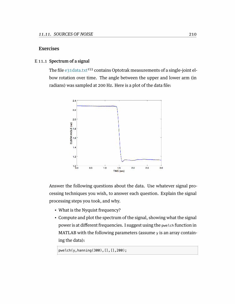
11.11. SOURCES OF NOISE 210
Exercises
E 11.1 Spectrum of a signal
The file e31data.txt153 contains Optotrak measurements of a single-joint el-bow rotation over time. The angle between the upper and lower arm (inradians) was sampled at 200 Hz. Here is a plot of the data file:
Answer the following questions about the data. Use whatever signal pro-cessing techniques you wish, to answer each question. Explain the signalprocessing steps you took, and why.
• What is the Nyquist frequency?• Compute and plot the spectrum of the signal, showing what the signal
power is at different frequencies. I suggest using the pwelch function inMATLAB with the following parameters (assume y is an array contain-ing the data):
pwelch(y,hanning(300),[],[],200);

11.11. SOURCES OF NOISE 211
Note that the Hanning function simply returns a vector of weights thatare applied to each window of data used in the pwelch function. It pro-vides a smoother spectrum. To visualize the Hanning window you cando this: plot(hanning(300)).
• What does the spectrum reveal about this signal?
E 11.2 Scoring kinematics
The file e31data.txt154 contains Optotrak measurements of a single-joint el-bow rotation over time. The angle between the upper and lower arm (inradians) was sampled at 200 Hz. Here is a plot of the data file:
Answer the following questions about the data. Use whatever signal pro-cessing techniques you wish, to answer each question. Explain the signalprocessing steps you took, and why.
• Determine theangle (indegrees) that theelbowrotatedover the courseof the arm movement.
• Determine the peak velocity, in radians per second, of the elbow move-ment. Hint: use the built-in MATLAB function gradient() to compute

11.11. SOURCES OF NOISE 212
the central difference so you don’t introduce a time lag and so thederivative has the same number of elements as the position array.
• Determine the peak positive and peak negative accelerations, in radi-ans per second per second.
E 11.3 Estimating your heart rate using your webcam or smartphone
In this exercise we will attempt to estimate your heart rate using a videotaken with your webcam or your smartphone.
Here’s what you will do to generate the data. First, make sure you’re ina brightly lit space (i.e. turn on the lights if you’re in a dark room!). Bet-ter yet, find a light source like a desk lamp and direct it at your webcam orsmartphone camera. Nowgently rest the tip of your indexfinger against thelens of your webcam or smartphone camera. Now start recording a video.Record for 30 seconds. Try not to move your finger, keep everything still.
If youusedyour smartphone, transfer thevideofile toyour computer. Openit up and look at it on the screen. Here’s a sample frame from mine, whichwas approximately 15 seconds in duration:

11.11. SOURCES OF NOISE 213
Here is a link to the example video: IMG_1383.MOV155
If you can’t make a video of your own, you are free to use my sample videoinstead, just download it to your machine.
The idea here is that as your heart pumps blood through your arteries andveins, the amount of light that the camera detects, as it comes through yourfingertip, will be modulated by the differences in blood flow. The variationin brightnesswill be subtle, and so your task is to use signal processing tech-niques to try to detect it.
Your task is to:
1. plot mean brightness over time as below2. estimate mean heart rate (in beats per minute) during your (or my)
video
Here are some suggestions as to how to proceed. Load in your video file,frame by frame. Each frame will have three channels: red, green and blue.

11.11. SOURCES OF NOISE 214
Each frame will contain the brightness of each pixel for each of the threechannels red, green and blue. You might as well average over all the pixelsin the frame to get an average brightness measure. The signal that you ulti-mately want is probably the brightness over time (i.e. for each frame of thevideo).
As an example, here is themean (over pixels) zero-centered brightness overtime, for my 15-sec example video (blue) and a band-pass filtered version(in red):
Here are some hints about how to implement this in MATLAB:
The MATLAB function VideoReader will load in a .MOV file. Here is somesample code:
video = VideoReader('IMG_1383.MOV');
nframes = video.NumberOfFrames;
frameHeight = video.Height;
frameWidth = video.Width;
frameRate = video.FrameRate; % frames per second
duration = video.Duration; % seconds

11.11. SOURCES OF NOISE 215
time = linspace(0,duration,nframes);
To read in a single frame of the video (for example the ith frame, you cando the following:
frame = read(video, i);
To get the mean brightness of the red channel you could do the following:
redChannel = frame(:, :, 1);
brt = mean(redChannel(:));
or to get the mean brightness across all channels in the frame:
brt = mean(frame(:));
What you probably want to do is implement a loop, going frame by frame,and in each frame, compute mean brightness, and store that (single) valuefor each frame, in an array.
Then you could band-pass filter this signal between frequencies of interest(e.g. a frequency range where you expect to see a heartbeat, e.g. 40–200bpm. Remember to convert beats per minute (bpm) to Hz before using thebandpass function.
The cutting edge (not needed for your assignment, just FYI)
In 2012, some researchers at MIT published a new method for amplifyingsubtle changes in motion (or other aspects of a video) and visualizing themover time:
Eulerian Video Magnification for Revealing Subtle Changes in the World156
It’s pretty cool stuff. See example videos:

11.11. SOURCES OF NOISE 216
• Revealing Invisible Changes in the World157 (layperson version)• Eulerian Video Magnification158 (more technical version)

LINKS 217
Links
133https://jackschaedler.github.io/circles-sines-signals/index.html
134http://en.wikipedia.org/wiki/Fourier_series
135http://bl.ocks.org/jinroh/7524988
136http://en.wikipedia.org/wiki/Fast_Fourier_transform
137https://youtu.be/NAsM30MAHLg
138https://www.youtube.com/watch?v=8KmVDxkia_w
139https://www.youtube.com/watch?v=6dW6VYXp9HM
140https://www.youtube.com/watch?v=jfH-NbsmvD4
141http://en.wikipedia.org/wiki/Nyquist–Shannon_sampling_theorem
142http://en.wikipedia.org/wiki/Aliasing
143http://en.wikipedia.org/wiki/Nyquist_frequency
144http://en.wikipedia.org/wiki/Aliasing
145http://www.mathworks.com/help/signal/ref/dspdata.psd.html
146http://en.wikipedia.org/wiki/Formant
147http://en.wikipedia.org/wiki/Bode_plot
148http://en.wikipedia.org/wiki/Filter_design
149http://en.wikipedia.org/wiki/Z-transform
150http://en.wikipedia.org/wiki/Transfer_function
151http://en.wikipedia.org/wiki/Digital_filter
152http://en.wikipedia.org/wiki/Low-pass_filter#Continuous-time_low-pass_filters
153http://www.gribblelab.org/scicomp/exercises/e31data.txt
154http://www.gribblelab.org/scicomp/exercises/e31data.txt
155http://www.gribblelab.org/scicomp/exercises/IMG_1383.MOV

LINKS 218
156http://people.csail.mit.edu/mrub/vidmag/
157http://youtu.be/e9ASH8IBJ2U
158http://youtu.be/ONZcjs1Pjmk

LINKS 219
Figure 11.10: Three filtered versions of a noisy signal with peaks at 6, 10 and 13 Hz, inthe time domain.

LINKS 220
Figure 11.11: Sample 3D movement data recorded from Optotrak at 200 Hz.
Figure 11.12: Sample 3D movement data recorded from Optotrak at 200 Hz, low-passfiltered using a 12 Hz cutoff frequency.

LINKS 221
Figure 11.13: A continuous signal sampled at a variety of (low) sampling rates, showingquantization.

LINKS 222

12 Optimization & gradient descent
In linear regression, we fit a line of best fit toN samples of (Xi,Yi) data (i = 1 . . .N)according to a linear equation with two parameters, β0 and β1:
Yi = β0 + β1Xi + εi (12.1)
To find the β parameters corresponding to the regression line, we can use a for-mula that’s based on a procedure called ordinary least squares (OLS). What OLSdoes is find the β parameters that minimize the sum of squared deviations of theestimated values of the data Y (using given values of β) and the actual values ofY. That is, the values of β0 and β1 that minimize Jwhere:
J =N∑i=1
(Yi − Yi
)2(12.2)
We can call this function J a cost function. The goal then, is to determine, some-how, the values of the parameters β0 and β1 that minimize the cost function J.
This is a classic example of an optimization problem. We want to optimize theparameters β so that they minimize the cost function J.
Optimization problems abound in science, data analysis, statistical modeling,and even out there in the real world. Here are a few examples, to help you so-lidify in your mind what optimization is all about, and how it may be used. For
223

224
someproblems (e.g. the shower example) it is easy to thinkabouthowyouwouldfind the optimal solution. For others, it is not immediately obvious.
• Your morning shower: A simple example of optimization is when you hopin the shower and turn on the hot and cold water taps. What you desire isa water temperature that is not too hot, not too cold, but “just right”. Theparameters to be optimized are the relative amounts of cold and hot watercoming out of the shower head. The cost function is how uncomfortable(whether too cold or too hot) the water temperature is for you.
• Tuning a radio: When you tune a radio (an analog radio) and you’re search-ing for a particular radio station, you are performing an optimization. Theparameter you are optimizing is the position of the tuner along the radiospectrum that spans the frequency of the radio station you are trying to lis-ten to. The cost function is the amount of static that you hear overtop ofthe radio station signal.
• Controlling rockets: NASA159 uses optimization techniques to determinethe trajectory of rockets and other spacecraft that will reach their destina-tionusing the least amount of fuel. In this case there are parameters that de-finedifferent trajectories, anda cost function that involves the total amountof fuel burn.
• Travelling salesman: A classic example of an optimization problem is theTravelling salesman problem160. Given a list of cities and the distances be-tween each pair of cities, what is the shortest possible route that visits eachcity exactly once and returns to the origin city? In this case the parametersto be optimized are the order of visiting each city, and the cost is the totaldistance travelled.
• Finance: Bankers perform portfolio optimization to determine the mixtureof investments that strike the best balance between risk and return. In thiscase the parameters are the proportions of each type of investment (stocks,

225
bonds, real estate, gold, etc) and the cost function is some (generally secret)equation that balances risk and return.
• Statistics: In statistics and data modelling, optimization can be used to findthe parameters of a model that best fits the observed data. In this case theparameters to be optimized are the parameters that define the particularmodel that is being used to model the data (e.g. for linear regression, the βvalues), and the cost function is some measure of goodness-of-fit (actually“badness” of fit). In the case of linear regression, the cost function J is givenabove.
• Machine Learning: Many methods in machine learning, including classifi-cation, prediction, etc, are based on optimization: finding the values ofmodel parameters that minimize some cost function. In logistic regression,support vector machines, etc, we find the parameter values that minimizethe errors in classifying inputs as belonging to one category vs another (e.g.spamvs non-spamemail, or benign vs cancerous tumours, etc). In artificialneural network models, we use optimization to find the values of neuron-to-neuron weights that minimize the network’s errors on an input-outputtraining set.
• The Brain?: Some people theorize that some brain functions (e.g. motorcontrol, perception) can be conceptualized as optimization problems. Forexample for motor cortex, the parameters to be optimized might be thetime-varying pattern of action potentials that arrive at α motoneurons inthe spinal cord (and hence activate muscles, and move the body) and thecost function might be the amount of beer that is spilled as you move thebeer stein from the tabletop to your mouth.
The big question then, is how to determine the parameters that minimize thecost function? There are two general approaches. The analytic approach is to tryto find an analytical expression that allows one to directly compute the optimal
12.1. ANALYTIC APPROACHES 226
parameter values. This is wonderful when it can be achieved, because direct cal-culation is fast. For linear regression using OLS, there exists a matrix equation(shown below) that provides an analytical solution.
For many problems however, it is not possible to find an analytical expressionthat gives the optimal parameter values. In these cases, one uses a numericalapproach to estimate the optimal parameter values (the parameter values thatminimize the cost function). As long as you can compute the value of the costfunction for a given set of parameter guesses, then you can pursue a numericalapproach to optimization. The downside of the numerical approach however isthat (1) it can take a long time to converge on the solution, and (2) for some prob-lems, it can be extremely difficult or practically infeasible to converge on the op-timal solution.
Optimization is a topic that people can (and have) spent their entire careersstudying. It is one of the most important topics in applied mathematics and en-gineering. We will not attempt to cover the topic in any great breadth. Our goalhere is to introduce you to the central idea, and to get some practical experienceusing numerical approaches to optimization.
12.1 Analytic Approaches
In the case of linear regression, there happens to be an analytical expression thatallows us to directly calculate the β values that minimize J. This is the formula,in matrix format:
β =(X⊤X
)−1X⊤Y (12.3)
In your undergraduate statistics class(es) you may have seen a simpler looking,non-matrix version of this:

12.1. ANALYTIC APPROACHES 227
β0 = Y− β1X (12.4)
β1 =
∑(Yi − Y) (Xi − X)∑(Xi − X)2 (12.5)
How do we come up with analytic expressions like these? The answer is Calcu-lus161.
It might help to understand the following material by considering a simpler op-timization problem, where we have a single paramater β to be optimized, for ex-ample the position of a radio tuner as you hone in on your favourite radio station.Call the position of the tuner dial β. What we want is to find the value of β thatminimizes the cost function J, where J is, for example, the amount of static thatyou hear overtop of the radio station signal. Let’s say we’re searching the air-waves for Virgin Radio but you’ve forgotten the frequency (97.5 MHz). We canvisualize a hypothetical relationship between β and J graphically, as shown inFigure 12.1.
Figure 12.1: Cost function for tuning a radio.
12.1. ANALYTIC APPROACHES 228
As we move the dial under or over the actual (forgotten) frequency for VirginRadio, we get static and the cost function J increases. The farther we move thedial away from the 97.5 MHz frequency, the greater the cost function J. What wedesire is the frequency (the value of β) corresponding to the bottom (minimum)of the cost function, i.e. the minimum value of J.
We can remember from our high school calculus days that at the minimum ofa function f, the first derivative162 of f equals zero. With respect to our VirginRadio example, this means that the derivative of Jwith respect to β is zero at theminimum of J. In equation form with calculus notation, what we want to deriveis an expression that gives us the value of β forwhich the first derivative of βwithrespect to J is zero:
∂J∂ β
= 0 (12.6)
If we can write an algebraic expression to describe how J varies with β, thenthere’s a chance that we can do the differentiation and arrive at an analytic ex-pression for the minimum. A very simple toy example: let’s say we can write J(β)as:
J = 10+ (β− 97.5)2 (12.7)
Now in this little example one doesn’t need calculus to see that the way to mini-mize J is to set β = 97.5. Let’s pretend however that we couldn’t see this solutiondirectly (as is often the case with more complex cost functions—for example forlinear regression and OLS). If we take the derivative of Jwith respect to β, we get:

12.1. ANALYTIC APPROACHES 229
∂J∂β = 0 (12.8)
∂[10+ (β− 97.5)2]∂β = 0 (12.9)
2 (β− 97.5) = 0 (12.10)
2β = 2(97.5) (12.11)
β = 97.5 (12.12)
So in this little example the analytical expression for the optimal value of β isn’teven an expression per se, it’s an actual value.
Note also that technically, that the slope of a function is zero not only at a min-imum but also at a peak. If we truly want to find only minima then we shouldalso look for places where the second derivative (the slope of the slope) is posi-tive. Parameter valueswhere thefirst derivative is zero and the secondderivativeis positive, correspond to valleys. Parameter values where the first derivative iszero and the second derivative is negative, correspond to peaks. Draw a functionwith a peak and a valley, then draw the first and second derivatives, to convinceyourself that this is true. See Figure 12.2 for an example of a functionwith a peakand a valley.
If youwant to seehow the solutions for β0 and β1 are derived, for linear regressionOLS, you can see this summary163 by Simon Jackman.
For some optimization problems, doing the calculus to find an analytical expres-sion for the optimal parameter values is possible. For many optimization prob-lems however, the calculus simply cannot be done. In this case our only optionis to pursue a numerical approach. This is what we will focus on in this course—numerical approaches to optimization.

12.2. NUMERICAL APPROACHES 230
Figure 12.2: Peak and valley.
12.2 Numerical Approaches
In numerical approaches to optimization, the general idea is that you pursue aniterative approach in which you guess at optimal parameter values, you evaluatethe cost, and then you revise your guess. This loop continues until you decideyou can no longer reduce the cost.
Numerical approaches canbedistinguishedas localversus globalmethods. Localmethods use only local information about the relationship between cost and pa-rameter values in the local “neighborhood”of the current guess. Globalmethodsinvolve multiple guesses over a broad range of parameter values, and revised pa-rameter guesses take into account information from all guesses across the entireparameter range.
12.2.1 Local methods
In local numerical approaches to optimization, the basic idea is to:

12.2. NUMERICAL APPROACHES 231
1. start with an initial guess at the optimal parameter values2. compute the cost at hose parameter values3. is the cost low enough? If yes, stop. If no, continue4. estimate the local gradient at the current parameter values5. take a step to new parameter values using the local gradient info6. go to step 2
Sometimes at step 2, the stopping rule looks at not just the current cost but alsoother values such as the magnitude of the local gradient. For example if the localgradient gets too shallow then the stopping rule might get triggered.
You can think of this all in real-world terms in the following way. Imagine you’reheli-skiing in the back-country, and at the end of the day instead of taking youback to Whistler village, your helicopter pilot drops you somewhere on the sideof Whistler Mountain164. Only problem is, it’s extremely foggy and you have noidea where you are, or which way is down to the village. You can only see 3 feetin front of you. All you have on you is an altimeter. What do you do? Probablysomething akin to the iterative numerical approach of gradient descent.
You have to decide which way is downhill, and then ski in that direction. To es-timate which way is downhill you could do something like the following: takea step in three directions around a circle, and for each step, check the altimeterand compare the altitude to the altitude at the center of the circle. The step cor-responding to the greatest altitude decrease represents the steepest “downhill”.
Then you have to decide how long to ski in that direction. You could even tailorthis ski time to the local gradient of the mountain. The steeper the slope, thesmaller the ski time. The shallower the slope, the longer the ski time.
When you determine thatmoving in any direction doesn’t decrease your altitudevery much, you conclude that you’re at the bottom.
This is essentially how numerical approaches to optimization work, by doing it-

12.2. NUMERICAL APPROACHES 232
erative gradient descent. Think about the ski hill example, and what kinds ofthings can go wrong with this procedure.
12.2.2 Local minima
One common challenge with complex optimization problems, is the issue of lo-calminima. In thebowl-shapedexample of a cost function thatweplotted above,there is a single global minimum to the cost function—one place on the cost land-scape where the slope is zero. It happens often however that there are local min-ima in the cost function—parameter values that correspond to a flat region of thecost function, where local steps will only increase the cost—but for which thecost is not the global minimum cost. Figure 12.3 shows an example of such acost function.
Figure 12.3: Local minimum.
You can see that there is a single global minimum at a parameter value of about-1—but there is a second, local minimum at a parameter value of about 2.2. Youcan see that if our initial parameter guess was between 1.5 and 3.0, that our localgradient descent procedure would put us at the local minimum, not the global

12.2. NUMERICAL APPROACHES 233
minimum.
One strategy to deal with local minima is to run several gradient descent runs,each starting from a different (often randomly chosen) initial parameter guess,and then to take the best one as the global minimum. Ultimately however inthe absence of an analytic solution, or a brute force mapping of the entire costlandscape (which is often infeasible) one can never be sure that one isn’t at alocal versus a global minimum.
12.2.3 Algorithms
A number of effective algorithms have been developed for finding parameter val-ues that minimize a cost function. Some don’t assume any pre-existing knowl-edge of the gradient—that is, of the derivative of the cost function with respect tothe parameters, while some assume that we can compute both the cost and thegradient for a given set of parameter values.
In simple gradient descent165, the simple idea is as described above, namely toestimate the local gradient and then take a step in the steepest direction. Thereare all sorts of ways of defining the step size, and adapting the step size to thesteepness of the local gradient. There are also terms one can add that implementmomentum166, as a scheme to try to avoid local minima. Another strategy is toinclude randomness, by implementing stochastic gradient descent167.
In conjugate gradient descent168, one requires knowledge of the local gradient,and the idea here is that the algorithm tries to compute a more intelligent guessas to the direction of the cost minimum.
In Newton’s method169, one approximates the local gradient using a quadraticfunction, and then a step is taken towards the minimum of that quadratic func-tion. Youcan thinkof this as a slightlymore sophisticatedversionof simple gradi-entdescent, inwhichoneessentially approximates the local gradient as a straight

12.2. NUMERICAL APPROACHES 234
line.
The Nelder-Mead (simplex) method170 is an iterative approach that is pretty ro-bust, that has an interesting geometric interpretation (see the animation on thewikipedia page) that is not unlike the old toy called Wacky Wally171.
There are more complex algorithms such as Levenberg-Marquardt172 and others,which we won’t get into here.
The bottom line is that there are a range of local methods that vary in their com-plexity, in theirmemory requirements, in their iteration speed, and their suscept-ability to getting stuck in local minima. My approach is to start with the simpleones, and add complexity when needed.
12.2.4 Global methods
In global optimization173, the general idea is instead of making a single guessand descending the local gradient, one instead makes a large number of guessesthat broadly span the range of the parameters, and one evaluates the cost forall of them. Then the update step uses the costs of the entire set of guesses todetermine a new set of guesses. It’s also an iterative procedure, and when thestopping rule is triggered, one takes the guess from the current set of guessesthat has the lowest cost, as the best estimate of the global minimum.
Global methods are well suited to problems that involve many local minima. Go-ing back to our ski hill example, imagine instead of dropping one person on theside of Whistler mountain, rather a platoon of paratroopers is dropped from aplane and scattered all over the entire mountain range. Some will end up in val-leys and alpine lakes (local minima) but the chances are good that at least onewill end up in whistler village, or close to it. They all radio up to the airplanewith their reported altitudes, and on the basis of an analysis of the entire set, anew platoon is dropped, and eventually, someone will end up at the bottom (the

12.3. OPTIMIZATION IN MATLAB 235
global minimum).
Two popular global methods you might come across are simulated annealing174
and genetic algorithms175. Read up on them.
12.3 Optimization in MATLAB
MATLAB has many different functions in the Optimization Toolbox for doing op-timization, depending on whether you are doing linear vs nonlinear optimiza-tion, whether you have constraints or your problem is unconstrained, and otherconsiderations as well. See the MATLAB documentation for all the details.
Here we will consider unconstrained nonlinear optimization, and later we willlook at curve fitting.
12.3.1 Unconstrained nonlinear optimization
There are two main functions to consider in MATLAB for doing uncon-strained, nonlinear optimization: fminsearch (which usese Nelder-Mead simplexsearch176) and fminunc (which uses gradients to search).
The MATLAB documentation contains some guidelines about when to use thesedifferent functions:
“fminsearch is generally less efficient than fminunc for problems of or-der greater than two. However, when the problem is highly discontin-uous, fminsearch might be more robust.”
There is also a page in theMATLABdocumentation that gives amore comprehen-sive set of guidelines for when to use different optimization algorithms:
Choosing a Solver177

12.3. OPTIMIZATION IN MATLAB 236
Here is a simple example of a one-dimensional (one parameter) optimizationproblem. Consider the following function J of a single parameter x:
J(x) = xe(−x2) +x220 (12.13)
Assume values of x range between -10.0 and +10.0.
Let’s first generate a plot of the cost function J over the range of x. The code isshown below and the plot is shown in Figure 12.4.
J = @(x) x.*exp(-x.^2) + (x.^2)/20;
x = -10:0.1:10;
y = J(x);
plot(x,y)
Figure 12.4: A function of a single variable.
We can see that there is a global minimum between -2.0 and 0.0, and there alsoappears tobea localminimumbetween0.0and3.0. Let’s tryusing the fminsearch

12.3. OPTIMIZATION IN MATLAB 237
function to find the value of xwhich minimizes J(x):
>> [X,FVAL,EXITFLAG] = fminsearch(J,0.0)
X =
-0.6691
FVAL =
-0.4052
EXITFLAG =
1
We can see that the optimizer found a minimum at x = −0.6691, and that at thatvalue of x, J(x) = −0.4052. It appears that the optimizer successfully found theglobal minimum and did not get fooled by the local minimum.
Let’s try a two-dimensional problem:
J(x, y) = xe(−x.2−y2) +x2 + y220 (12.14)
Now we have a cost function J in terms of two variables x and y. Our problem isto find the vector (x, y) that minimizes J(x, y).
Let’s write a function file for our cost function:
function J = mycostfun2d(X)
%
% note use of dot notation on .* and ./ operators

12.3. OPTIMIZATION IN MATLAB 238
% this enables the computation to happen for
% vector values of x
%
x = X(:,1);
y = X(:,2);
J = (x .* exp(-(x.*x)-(y.*y))) + (((x.*x)+(y.*y))./20);
Let’s plot the cost landscape, which is shown in Figure 12.5:
x = linspace(-3,3,51); % sample from -3 to +3 in 50 steps
y = linspace(-3,3,51);
XY = combvec(x,y);
J = mycostfun2d(XY'); % compute cost function over all values
[Y,X] = meshgrid(x,y); % reshape into matrix form
Z = reshape(J,length(x),length(y));
figure % visualize the cost landscape
meshc(X,Y,Z);
shading flat
xlabel('X');
ylabel('Y');
zlabel('J');
Now let’s use fminsearch to find the values (x, y) that minimize J(x, y):
>> [Xf,FVAL] = fminsearch('mycostfun2d', [5,5])
Xf =
-0.6690 -0.0000
FVAL =
-0.4052

12.3. OPTIMIZATION IN MATLAB 239
Figure 12.5: Cost function landscape for a 2D problem.
Let’s plot our solution to verify it looks reasonable—this is shown in Figure 12.6:
hold on
z0 = get(gca,'zlim');
z0 = z0(1);
plot3([Xf(1),Xf(1)],[get(gca,'ylim')],[z0 z0],'color','r','linewidth',2);
plot3([get(gca,'xlim')],[Xf(2),Xf(2)],[z0 z0],'color','r','linewidth',2);
12.3.2 Curve Fitting
We can do nonlinear least squares curve fitting in MATLAB using lsqcurvefit.There is also a GUI tool for curve fitting in MATLAB called cftool.

12.3. OPTIMIZATION IN MATLAB 240
Figure 12.6: Cost function landscape for a 2D problem.
Exercises
E 12.1 Curve Fitting
Here are 10 pairs of (x,y) data:
x = [ 1, 2, 3, 4, 5, 6, 7, 8, 9, 10];
y = [18, 5, 17, 38, 40, 106, 188, 234, 344, 484];
Your task is to fit a function to the data. The function has the form:
yi = β0 + β1xi + β2x2i + β3x3i (12.15)
and the cost function J is:
J =10∑i=1
(yi − yi)2 (12.16)

12.3. OPTIMIZATION IN MATLAB 241
Usewhateveroptimizeryouwish. Plot thedataas a scatterplotof xvsy, andplot the function that corresponds to the parameter values β that minimizeJ.
E 12.2 Local Minima
Generate some noisy (x,y) data using the following MATLAB code:
x = 0:0.01:3;
y = sin(2*pi*x) + randn(size(x))*0.5;
Generate a scatterplot of the data, plotting x on the abscissa and y on theordinate.
Your task is to fit a function of the following form to the data:
y = sin(βx) (12.17)
The (single) parameter to be optimized is β. Your cost function J is:
J =n∑i=1
(yi − yi)2 (12.18)
where n is the number of (x,y) pairs in the data.
• Compute the cost function J for values of β ranging from -10.0 to +10.0,and plot the cost landscape (plot J as a function of β)
• Use anoptimizationmethodof your choosing tofind the value of β thatminimizes the cost function J. Plot the data and the overlay the bestfitting function. Justify that you have found a global minimum andnot a local minimum.
E 12.3 Egg Carton

12.3. OPTIMIZATION IN MATLAB 242
Assume your cost function J is the following function of two parameters(x,y):
J(x, y) = −20eA − eB + 20+ e (12.19)
where
A = −0.2√0.5(x2 + y2) (12.20)
and
B = 0.5 [cos(2πx) + cos(2πy)] (12.21)
• Compute the cost function J for values of (x, y) ranging from -10.0 to10.0, and plot the cost landscape (plot J as a function of (x, y)). hint:Hint: it should look something like [this178
• Usewhatever optimizationmethod youwish, to find the values of (x, y)that minimize the cost function J. Justify that you have found theglobal minimum and not a local minimum

LINKS 243
Links
159http://www.nasa.gov
160http://en.wikipedia.org/wiki/Travelling_salesman_problem
161http://en.wikipedia.org/wiki/Calculus
162http://en.wikipedia.org/wiki/Derivative
163http://jackman.stanford.edu/classes/ssmart/2011/derive1.pdf
164http://www.whistlerblackcomb.com/the-mountain/weather-and-mountain-stats.aspx
165http://en.wikipedia.org/wiki/Gradient_descent
166http://www.willamette.edu/~gorr/classes/cs449/momrate.html
167http://en.wikipedia.org/wiki/Stochastic_gradient_descent
168http://en.wikipedia.org/wiki/Conjugate_gradient_method
169http://en.wikipedia.org/wiki/Newton's_method_in_optimization
170http://en.wikipedia.org/wiki/Nelder%E2%80%93Mead_method
171http://youtu.be/l8Dbne0wRaE?t=18s
172http://en.wikipedia.org/wiki/Levenberg–Marquardt_algorithm
173http://en.wikipedia.org/wiki/Global_optimization
174http://en.wikipedia.org/wiki/Simulated_annealing
175http://en.wikipedia.org/wiki/Genetic_algorithm
176https://en.wikipedia.org/wiki/Nelder–Mead_method
177http://www.mathworks.com/help/optim/ug/choosing-a-solver.html
178http://wolfr.am/85VNivEU

LINKS 244

13 Integrating ODEs & simulating
dynamical systems
13.1 What is a dynamical system?
Systems can be characterized by the specific relation between their input(s) andoutput(s). A static system has an output that only depends on its input. A me-chanical example of such a system is an idealized, massless spring. The lengthof the spring depends only on the force (the input) that acts upon it. Changethe input force, and the length of the spring will change, and this will happen in-stantaneously (obviously a massless spring is a theoretical construct). A systembecomes dynamical (it is said to have dynamics) when a mass is attached to thespring (Figure 13.1 below). Now the position of the mass (and equivalently, thelength of the spring) is no longer directly dependent on the input force, but isalso tied to the acceleration of the mass, which in turn depends on the sum of allforces acting upon it (the sum of the input force and the force due to the spring).The net force depends on the position of the mass, which depends on the lengthof the spring, which depends on the spring force. The property that accelerationof the mass depends on its position makes this a dynamical system.
Dynamical systems can be characterized by differential equations that relate thestate derivatives (e.g. velocity or acceleration) to the state variables (e.g. posi-tion). The differential equation for the spring-mass system depicted above is:
245
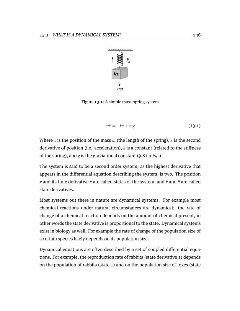
13.1. WHAT IS A DYNAMICAL SYSTEM? 246
Figure 13.1: A simple mass-spring system
mx = −kx+mg (13.1)
Where x is the position of the mass m (the length of the spring), x is the secondderivative of position (i.e. acceleration), k is a constant (related to the stiffnessof the spring), and g is the graviational constant (9.81 m/s/s).
The system is said to be a second order system, as the highest derivative thatappears in the differential equation describing the system, is two. The positionx and its time derivative x are called states of the system, and x and x are calledstate derivatives.
Most systems out there in nature are dynamical systems. For example mostchemical reactions under natural circumstances are dynamical: the rate ofchange of a chemical reaction depends on the amount of chemical present, inother words the state derivative is proportional to the state. Dynamical systemsexist in biology as well. For example the rate of change of the population size ofa certain species likely depends on its population size.
Dynamical equations are often described by a set of coupled differential equa-tions. For example, the reproduction rate of rabbits (state derivative 1) dependson the population of rabbits (state 1) and on the population size of foxes (state

13.2. WHY MAKE MODELS? 247
2). The reproduction rate of foxes (state derivative 2) depends on the popula-tion of foxes (state 2) and also on the population of rabbits (state 1). In this casewe have two coupled first-order differential equations, and hence a system of or-der two. The so-called predator-prey model is also known as the Lotka-Volterraequations179:
x = x(α− βy) (13.2)
y = −y(γ− δx) (13.3)
13.2 Why make models?
There are two main reasons why we would want to model a physical systemusing mathematical equations, one being practical and one mostly theoretical.The practical use is prediction. A typical example of a dynamical system thatis modelled for prediction is the weather. The weather is a very complex, (high-order, nonlinear, coupled and chaotic) system. More theoretically, one reason tomake models is to test the validity of a functional hypothesis of an observed phe-nomenon. A beautiful example is the model made by Hodgkin and Huxley180
to understand how action potentials arise and propagate in neurons (see Fig-ures 13.2 and 13.3 below). Theymodelled the different (voltage-gated) ion chan-nels in an axon membrane and showed using mathematical models that indeedthe changes in ion concentrations were responsible for the electical spikes ob-served experimentally 7 years earlier.
A second theoretical reason to make models is that it is sometimes very difficult,if not impossible, to answer a certain question empirically. As an example wetake the following biomechanical question: Would you be able to jump higher ifyour biceps femoris (part of your hamstrings) were two separate muscles eachcrossing only one joint rather than being one muscle crossing both the hip and

13.2. WHY MAKE MODELS? 248
Figure 13.2: Hodgkin-Huxley model of voltage-gated ion channels
knee joint? Not a strange question as one could then independently control thetorques around each joint.
In order to answer this question empirically, one would like to do the followingexperiment:
• measure the maximal jump height of a subject• change only the musculoskeletal properties in question• measure the jump height again
Of course, such an experiment would yield several major ethical, practical andtheoretical drawbacks. It is unlikely that an ethics committee would approve thetransplantation of the origin and insertion of the hamstrings in order to examineits effect on jump height. And even so, one would have some difficulties find-ing subjects. Even with a volunteer for such a surgery it would not bring us anycloser to an answer. After such a surgery, the subject would not be able to jumpright away, but would have to undergo significant rehabilitation, and surely dur-
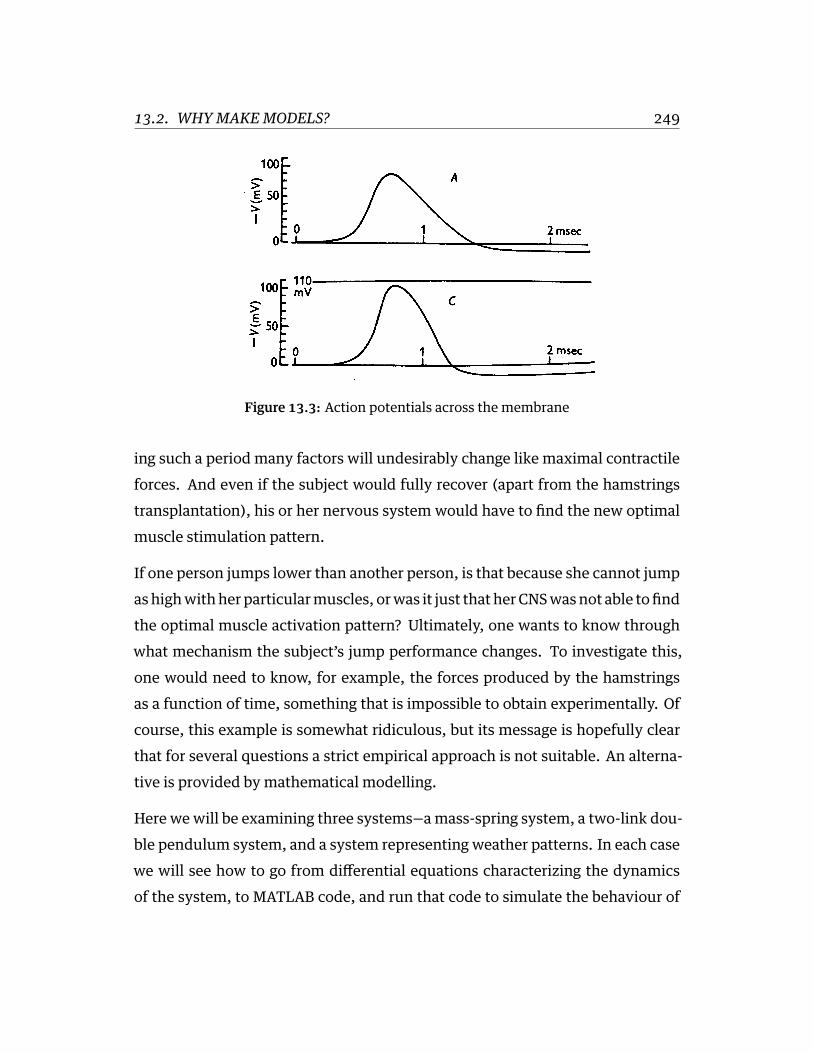
13.2. WHY MAKE MODELS? 249
Figure 13.3: Action potentials across the membrane
ing such a period many factors will undesirably change like maximal contractileforces. And even if the subject would fully recover (apart from the hamstringstransplantation), his or her nervous system would have to find the new optimalmuscle stimulation pattern.
If one person jumps lower than another person, is that because she cannot jumpashighwithher particularmuscles, orwas it just that herCNSwasnot able tofindthe optimal muscle activation pattern? Ultimately, one wants to know throughwhat mechanism the subject’s jump performance changes. To investigate this,one would need to know, for example, the forces produced by the hamstringsas a function of time, something that is impossible to obtain experimentally. Ofcourse, this example is somewhat ridiculous, but its message is hopefully clearthat for several questions a strict empirical approach is not suitable. An alterna-tive is provided by mathematical modelling.
Here we will be examining three systems—a mass-spring system, a two-link dou-ble pendulum system, and a system representing weather patterns. In each casewe will see how to go from differential equations characterizing the dynamicsof the system, to MATLAB code, and run that code to simulate the behaviour of

13.3. MODELLING DYNAMICAL SYSTEMS 250
the system over time. We will see the great power of simulation, namely the abil-ity to change aspects of the system at will, and simulate to explore the resultingchange in system behaviour.
13.3 Modelling Dynamical Systems
13.3.1 Characterizing a System Using Differential Equations
A dynamical system such as the mass-spring system we saw before, can be char-acterized by the relationship between state variables s and their (time) deriva-tives s. How do we arrive at the correct characterization of this relationship? Theshort answer is, we figure it out using our knowledge of physics, or we are simplygiven the equations by someone else. Let’s look at a simple mass-spring systemagain, shown in Figure 13.4.
Figure 13.4: A spring with a mass attached
We know a couple of things about this system. We know from Hooke’s law181 ofelasticity that the extension of a spring is directly and linearly proportional to theload applied to it. More precisely, the force that a spring applies in response to aperturbation from it’s resting length (the length at which it doesn’t generate anyforce), is linearly proportional, through a constant k, to the difference in lengthbetween its current length and its resting length (let’s call this distance x). Forconvention let’s assumepositive values of x correspond to lengthening the spring

13.3. MODELLING DYNAMICAL SYSTEMS 251
beyond its resting length, and negative values of x correspond to shortening thespring from its resting length.
F = −kx (13.4)
Let’s decide that the state variable that we are interested in for our system is x.We will refer to x instead of s from now on to denote our state variable.
We also know from Newton’s laws of motion182 (specifically Newton’s secondlaw183) that the net force on an object is equal to its mass m multiplied by itsacceleration a (the second derivative of position).
F = ma (13.5)
Instead of using a to denote acceleration let’s use a different notation, in termsof the spring’s perturbed length x. The rate of change (velocity) is denoted x andthe rate of change of the velocity (i.e. the acceleration) is denoted x.
F = mx (13.6)
We also know that the mass is affected by two forces: the force due to the spring(−kx) and also the gravitational force g. So the equation characterizing the netforces on the mass is
∑F = mx = −kx+mg (13.7)
or just
mx = −kx+mg (13.8)
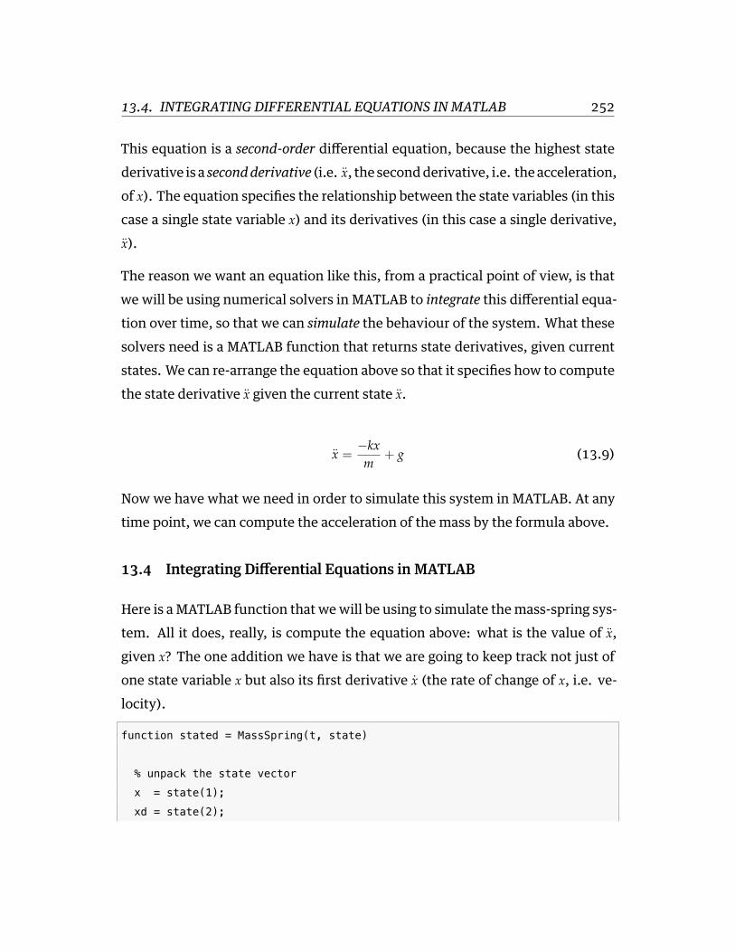
13.4. INTEGRATING DIFFERENTIAL EQUATIONS IN MATLAB 252
This equation is a second-order differential equation, because the highest statederivative is a secondderivative (i.e. x, the secondderivative, i.e. theacceleration,of x). The equation specifies the relationship between the state variables (in thiscase a single state variable x) and its derivatives (in this case a single derivative,x).
The reason we want an equation like this, from a practical point of view, is thatwe will be using numerical solvers in MATLAB to integrate this differential equa-tion over time, so that we can simulate the behaviour of the system. What thesesolvers need is a MATLAB function that returns state derivatives, given currentstates. We can re-arrange the equation above so that it specifies how to computethe state derivative x given the current state x.
x =−kxm + g (13.9)
Now we have what we need in order to simulate this system in MATLAB. At anytime point, we can compute the acceleration of the mass by the formula above.
13.4 Integrating Differential Equations in MATLAB
Here is a MATLAB function that we will be using to simulate the mass-spring sys-tem. All it does, really, is compute the equation above: what is the value of x,given x? The one addition we have is that we are going to keep track not just ofone state variable x but also its first derivative x (the rate of change of x, i.e. ve-locity).
function stated = MassSpring(t, state)
% unpack the state vector
x = state(1);
xd = state(2);

13.4. INTEGRATING DIFFERENTIAL EQUATIONS IN MATLAB 253
% these are our constants
k = 2.5; % Newtons per metre
m = 1.5; % Kilograms
g = 9.8; % metres per second
% compute acceleration xdd
xdd = ((-k*x)/m) + g;
stated = [xd, xdd];
end
Note that the function we wrote takes two arguments as inputs: state and t,which corresponds to time. This is necessary for the numerical solver that wewill use in MATLAB. The state variable is actually an array of two values corre-sponding to x and x.
How does numerical integration (simulation) work? Here is a summary of thesteps that a numerical solver takes. First, you have to provide the system withtwo things:
1. initial conditions (what are the initial states of the system?)2. a time vector over which to simulate
Given this, the numerical solver will go through the following steps to simulatethe system:
• calculate state derivatives x at the initial time (t = 0) given the initial states(x, x)
• estimate x(t+ Δt) using x(t = 0), x(t = 0) and x(t = 0)• calculate x(t = t+ Δt) from x(t = t+ Δt) and x(t = t+ Δt)• estimate x(t+2Δt) and x(t+2Δt)using x(t = t+Δt), x(t = t+Δt) and x(t = t+Δt)

13.4. INTEGRATING DIFFERENTIAL EQUATIONS IN MATLAB 254
• calculate x(t = t+ 2Δt) from x(t = t+ 2Δt) and x(t = t+ 2Δt)• … etc
In this way the numerical solver can esimate how the system states (x, x) unfoldover time, given the initial conditions, and the known relationship between statederivatives and system states. The details of the “estimate” steps above are notsomething we are going to dive into now. Suffice it to say that current estimationalgorithms are based on the work of two German mathematicians named Rungeand Kutta184 in the beginning of the 20th century. These numerical recipies arereadily available in MATLAB and are known as ODE solvers (ODE stands for ordi-nary differential equation).
Here’s how we would simulate the mass-spring system above. Assume that wehave the function MassSpring.m defined as above:
state0 = [0.0, 0.0];
t = 0:.1:10;
[t,state] = ode45('MassSpring', t, state0);
plot(t, state)
xlabel('TIME (sec)')
ylabel('STATES')
title('Mass-Spring System')
legend({'$x$ (m)', '$\dot{x}$ (m/sec)'},'interpreter','latex')
A couple of notes about the code. I have simply chosen, out of the blue, valuesfor the constants k and m. The gravitational constant185 g is of course known. Ihave also chosen to simulate the system for 10 seconds, and I have chosen a timeresolution of 100 milliseconds (0.1 seconds). We will talk later about the issue ofwhat is an appropriate time resolution for simulation.
You should see a plot like the one shown in Figure 13.5 below.
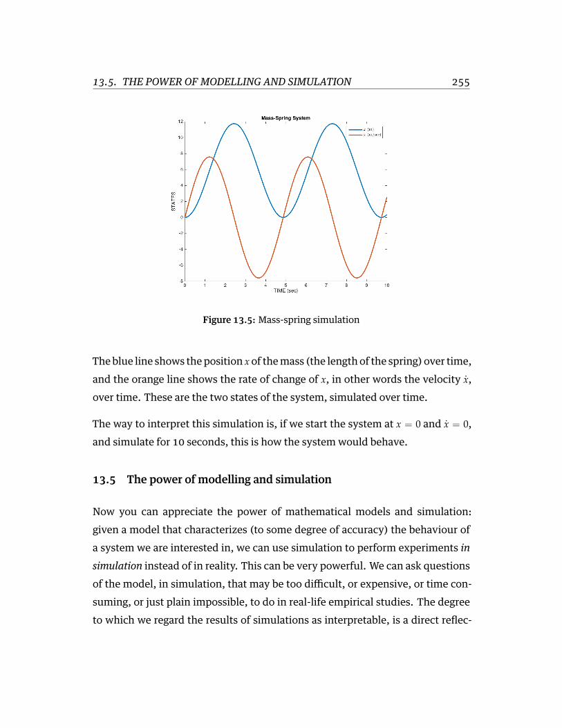
13.5. THE POWER OF MODELLING AND SIMULATION 255
Figure 13.5: Mass-spring simulation
Theblue line shows theposition xof themass (the length of the spring) over time,and the orange line shows the rate of change of x, in other words the velocity x,over time. These are the two states of the system, simulated over time.
The way to interpret this simulation is, if we start the system at x = 0 and x = 0,and simulate for 10 seconds, this is how the system would behave.
13.5 The power of modelling and simulation
Now you can appreciate the power of mathematical models and simulation:given a model that characterizes (to some degree of accuracy) the behaviour ofa system we are interested in, we can use simulation to perform experiments insimulation instead of in reality. This can be very powerful. We can ask questionsof the model, in simulation, that may be too difficult, or expensive, or time con-suming, or just plain impossible, to do in real-life empirical studies. The degreeto which we regard the results of simulations as interpretable, is a direct reflec-
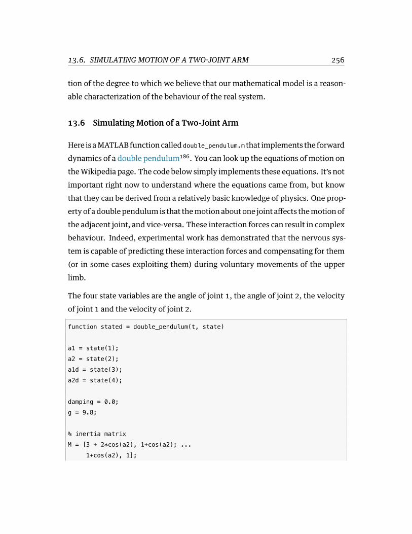
13.6. SIMULATING MOTION OF A TWO-JOINT ARM 256
tion of the degree to which we believe that our mathematical model is a reason-able characterization of the behaviour of the real system.
13.6 Simulating Motion of a Two-Joint Arm
Here is aMATLAB functioncalled double_pendulum.m that implements the forwarddynamics of a double pendulum186. You can look up the equations of motion ontheWikipedia page. The code below simply implements these equations. It’s notimportant right now to understand where the equations came from, but knowthat they can be derived from a relatively basic knowledge of physics. One prop-ertyof adoublependulum is that themotionaboutone joint affects themotionofthe adjacent joint, and vice-versa. These interaction forces can result in complexbehaviour. Indeed, experimental work has demonstrated that the nervous sys-tem is capable of predicting these interaction forces and compensating for them(or in some cases exploiting them) during voluntary movements of the upperlimb.
The four state variables are the angle of joint 1, the angle of joint 2, the velocityof joint 1 and the velocity of joint 2.
function stated = double_pendulum(t, state)
a1 = state(1);
a2 = state(2);
a1d = state(3);
a2d = state(4);
damping = 0.0;
g = 9.8;
% inertia matrix
M = [3 + 2*cos(a2), 1+cos(a2); ...
1+cos(a2), 1];

13.6. SIMULATING MOTION OF A TWO-JOINT ARM 257
% coriolis, centripetal and gravitational forces
c1 = a2d*((2*a1d) + a2d)*sin(a2) + ...
2*g*sin(a1) + g*sin(a1+a2);
c2 = -(a1d^2)*sin(a2) + g*sin(a1+a2);
% passive dynamics
cc = [c1-damping*a1d; ...
c2-damping*a2d];
% compute accelerations
acc = M\cc;
stated = [a1d a2d acc(1) acc(2)]';
end
Now that we have a function that implements the equations of motion, now wecan runa simulation, by starting the armout at some initial condition (initial jointangles and initial joint velocities) and integrating the differential equations overtime (using MATLAB’s ode45 function). Here is some MATLAB code for runninga simulation from a given set of initial state conditions, and animating the resultin a figure window. You’ll need this helper function called a2h.m as well:
function [h0,h1,h2] = a2h(a1,a2)
h0 = [0,0];
h1 = [sin(a1), cos(a1)];
h2 = [sin(a1) + sin(a1+a2), ...
cos(a1) + cos(a1+a2)];
end

13.6. SIMULATING MOTION OF A TWO-JOINT ARM 258
Here is the script for running the simulation and generating the animation:
%% run a simulation of a double pendulum
t = 0:.01:10;
x0 = [pi, pi/2, 0, 0];
[t,x] = ode45('double_pendulum', t, x0);
%% plot states over time
figure
plot(t,x)
%% run an animation
figure('position',[62 855 965 333]);
subplot(1,2,1)
plot(t,x(:,1:2))
legend({'a1','a2'})
hold on
s1ylim = get(gca,'ylim');
tline = plot([0 0],s1ylim,'r-','linewidth',1);
subplot(1,2,2)
[h0,h1,h2] = a2h(x(1,1),x(1,2));
l1 = plot([h0(1) h1(1)],[h0(2) h1(2)],'b-');
hold on
l2 = plot([h1(1) h2(1)],[h1(2) h2(2)],'b-');
axis([-2.2 2.2 -2.2 2.2]); axis equal
p0 = plot(h0(1),h0(2),'k.','markersize',15);
p1 = plot(h1(1),h1(2),'b.','markersize',15);
p2 = plot(h2(1),h2(2),'r.','markersize',15);
tp = title(sprintf('%5.1f',t(1)));
skip = 3;
for i=1:skip:length(t)
subplot(1,2,1)

13.6. SIMULATING MOTION OF A TWO-JOINT ARM 259
set(tline, 'Xdata', [t(i) t(i)]);
set(tline, 'Ydata', s1ylim);
subplot(1,2,2)
[h0,h1,h2] = a2h(x(i,1), x(i,2));
set(l1, 'XData', [h0(1) h1(1)]);
set(l1, 'YData', [h0(2) h1(2)]);
set(l2, 'XData', [h1(1) h2(1)]);
set(l2, 'YData', [h1(2) h2(2)]);
set(p1, 'XData', h1(1));
set(p1, 'YData', h1(2));
set(p2, 'XData', h2(1));
set(p2, 'YData', h2(2));
set(tp, 'String', sprintf('%5.1f', t(i)));
axis([-2.2 2.2 -2.2 2.2]);
drawnow;
end
What you see is a window with the time-varying angles on the left panel and ananimation of the double pendulum on the right panel, as in Figure 13.6.
Play with the simulation code and see what happens when you start the simula-tion from different initial conditions, for example different initial joint angles.
The simple model described here has only passive motion, there are no activeforces (for example generated by muscles). One can relatively easily add math-ematical models of muscle force generation, and other neurophysiologically rel-evant properties such as muscle mechanics, spinal reflex circuitry, reflex timedelays, and so on. One can then use such a model to test hypotheses about howthe brain controls voluntary arm movement.

13.7. LORENZ ATTRACTOR 260
Figure 13.6: Double pendulum
13.7 Lorenz Attractor
The Lorenz system187 is a dynamical system that we will look at briefly, as it willallow us to discuss several interesting issues around dynamical systems. It is asystemoftenused to illustrate non-linear systems188 theory and chaos theory189.It’s sometimes used as a simple demonstration of the butterfly effect190 (sensi-tivity to initial conditions). See here191 for a YouTube video that explains themeaning of the x, y and z coordinates.
The Lorenz system is a simplified mathematical model for atmospheric convec-tion. Let’s not worry about the details of what it represents, for now the impor-tant things to note are that it is a system of three /coupled/ differential equations,and characterizes a system with three state variables (x, y, z).

13.7. LORENZ ATTRACTOR 261
x = σ(y− x) (13.10)
y = (ρ− z)x− y (13.11)
z = xy− βz (13.12)
If you set the three constants (σ, ρ, β) to specific values, the system exhibitschaotic behaviour.
σ = 10 (13.13)
ρ = 28 (13.14)
β =83 (13.15)
Let’s implement this system in MATLAB. We have been given above the threeequations that characterize how the state derivatives (x, y, z) depend on (x, y, z)and the constants (σ, ρ, β). All we have to do is write a function that implementsthis, set some initial conditions, decide on a time array to simulate over, and runthe simulation using ode45(). First the function myLorenz.m that defines the dif-ferential equations:
function stated = myLorenz(t, state)
x = state(1);
y = state(2);
z = state(3);
% these are our constants
sigma = 10.0;
rho = 28.0;
beta = 8/3;
% compute the state derivatives

13.7. LORENZ ATTRACTOR 262
xd = sigma * (y-x);
yd = (rho-z)*x - y;
zd = x*y - beta*z;
% return the state derivatives
stated = [xd, yd, zd]';
end
Now the code to run the simulation:
state0 = [2.0, 3.0, 4.0];
t = 0:.01:30;
[t,state] = ode45('myLorenz', t, state0);
% plot the resuling state-space trajectory in 3D
plot(state(:,1), state(:,2), state(:,3))
xlabel('X'); ylabel('Y'); zlabel('Z');
grid on
You should see something like the plot shown in Figure 13.7 below.
The three axes on the plot represent the three states (x, y, z) plotted over the 30seconds of simulated time. We started the system with three particular values of(x, y, z) (I chose them arbitrarily), and we set the simulation in motion. This is thetrajectory, in state-space, of the Lorenz system.
You can see an interesting thing … the system seems to have two stable equilib-rium states, or attractors: those circular paths. The system circles around in one“neighborhood” in state-space, and then flips over and circles around the secondneighborhood. The number of times it circles in a given neighborhood, and thetime at which it switches, displays chaotic behaviour, in the sense that they areexquisitly sensitive to initial conditions.
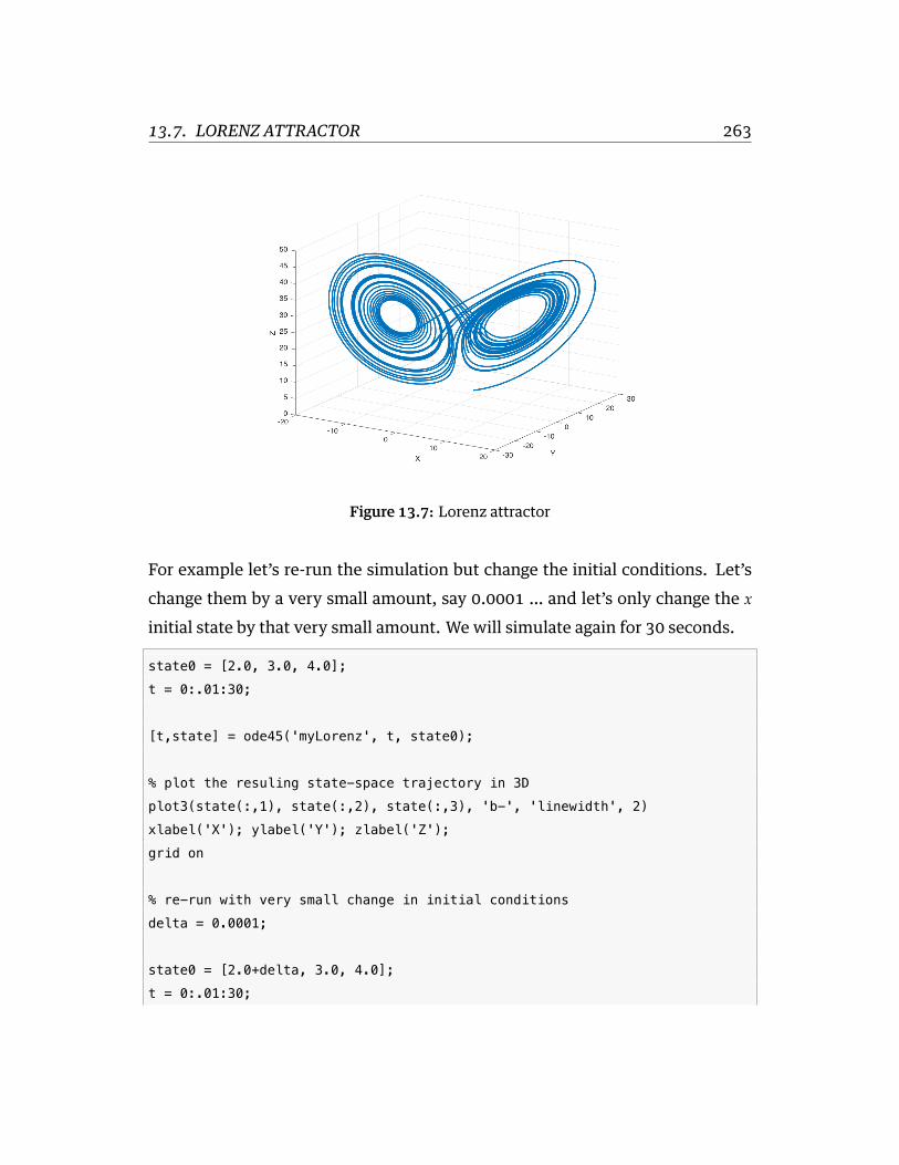
13.7. LORENZ ATTRACTOR 263
Figure 13.7: Lorenz attractor
For example let’s re-run the simulation but change the initial conditions. Let’schange them by a very small amount, say 0.0001 … and let’s only change the xinitial state by that very small amount. We will simulate again for 30 seconds.
state0 = [2.0, 3.0, 4.0];
t = 0:.01:30;
[t,state] = ode45('myLorenz', t, state0);
% plot the resuling state-space trajectory in 3D
plot3(state(:,1), state(:,2), state(:,3), 'b-', 'linewidth', 2)
xlabel('X'); ylabel('Y'); zlabel('Z');
grid on
% re-run with very small change in initial conditions
delta = 0.0001;
state0 = [2.0+delta, 3.0, 4.0];
t = 0:.01:30;

13.7. LORENZ ATTRACTOR 264
[t2,state2] = ode45('myLorenz', t, state0);
hold on
plot3(state2(:,1), state2(:,2), state2(:,3), 'r-', 'linewidth', 2)
You should see something like what is shown in Figure 13.8 below.
Figure 13.8: Lorenz attractor changing initial conditions
You can sort of see that at some point the two state-space trajectories diverge.You can better visualize this by plotting each state against time as shown in Fig-ure 13.9.
But let’s go one step further, let’s plot the distance between each point in state-space as a function of time:
dist = sqrt(sum((state2-state).^2,2));
figure
plot(t,dist,'b-','linewidth',2)
xlabel('TIME (sec)')
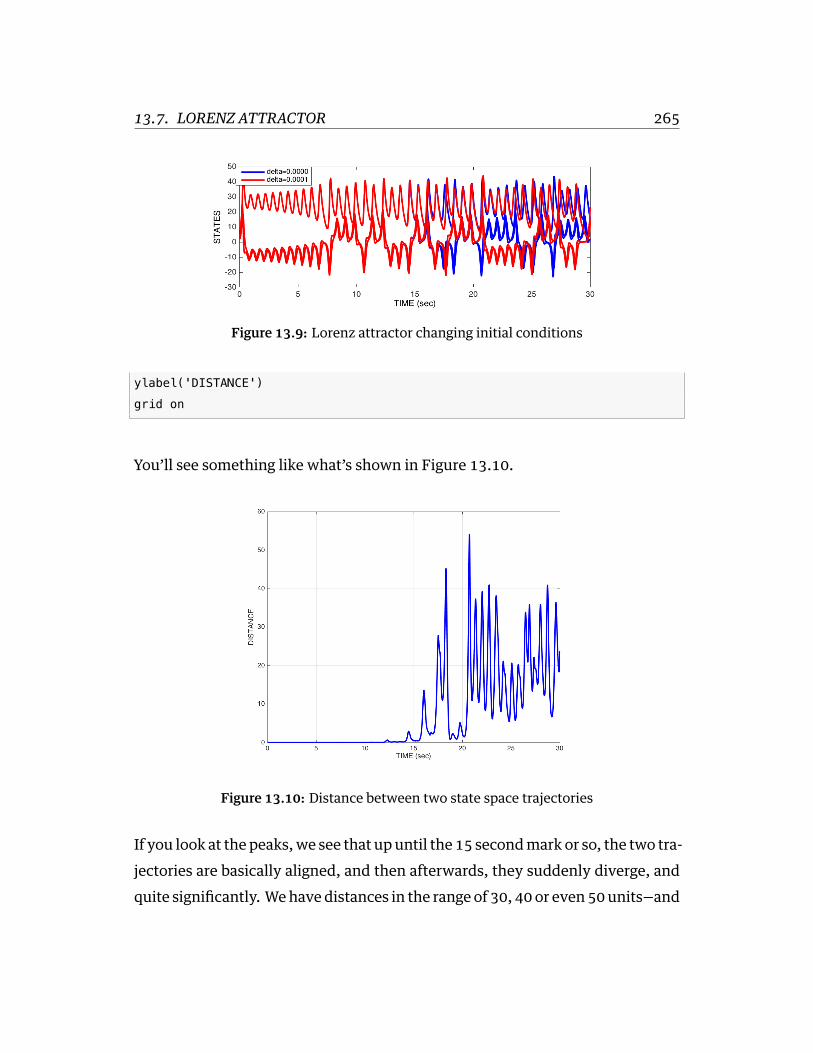
13.7. LORENZ ATTRACTOR 265
Figure 13.9: Lorenz attractor changing initial conditions
ylabel('DISTANCE')
grid on
You’ll see something like what’s shown in Figure 13.10.
Figure 13.10: Distance between two state space trajectories
If you look at the peaks,we see that upuntil the 15 secondmark or so, the two tra-jectories are basically aligned, and then afterwards, they suddenly diverge, andquite significantly. Wehavedistances in the range of 30, 40 or even50units—and

13.7. LORENZ ATTRACTOR 266
remember, this is generated with a difference in initial conditions of only 0.0001.That’s a 500,000x change.
Here’s some MATLAB code to generate an animation:
figure
plot3(state(:,1),state(:,2),state(:,3),'b-');
hold on
plot3(state2(:,1),state2(:,2),state2(:,3),'r-');
p1 = plot3(state(1,1),state(1,2),state(1,3),'b.','markersize',30);
p2 = plot3(state2(1,1),state2(1,2),state2(1,3),'r.','markersize',30);
tt = title('0.0');
step = 3;
view([32 22])
grid on
xlabel('X'); ylabel('Y'); zlabel('Z');
drawnow
for i=1:step:length(t)
set(p1,'XData',state(i,1));
set(p1,'YData',state(i,2));
set(p1,'ZData',state(i,3));
set(p2,'XData',state2(i,1));
set(p2,'YData',state2(i,2));
set(p2,'ZData',state2(i,3));
set(tt,'String',sprintf('%6.2f',t(i)));
drawnow
end
You should see an animation of the two state-space trajectories.
The original simulation is shown in blue. The simulation with the altered initialcondition is in red. Then an animated filled circle shows the state space overtime for the original (blue) and new (red, in which the initial condition of x wasincreasedby0.0001). The two followeachother quite closely for a long time, and

13.7. LORENZ ATTRACTOR 267
thenbegin todivergeat about the16 secondmark. At the20.76 secondmark theylook like what’s shown in Figure 13.11.
Figure 13.11: Animation of two Lorenz attractors
Note how the two systems are in different neighborhoods entirely!
This has illustrated how systems with relatively simple differential equationscharacterizing their behaviour, can turn out to be exquisitely sensitive to initialconditions. Just imagine if the initial conditions of your simulation were gath-ered from empirical observations (like the weather, for example). Now imagineyou use a model simulation to predict whether it will be sunny (left-hand neigh-borhoodof theplot above)or thunderstorms (right-handneighborhood), 30daysfrom now. If the answer can flip between one prediction and the other, based ona 1/10,000 different in measurement, you had better be sure of your empiricalmeasurement instruments, when you make a prediction 30 days out! Actuallythis won’t even solve the problem, no matter how precise your measurements.

13.7. LORENZ ATTRACTOR 268
The point is that the system as a whole is very sensitive to even tiny changes ininitial conditions. This is one reason why short-term weather forecasts are rela-tively accurate, but forecasts past a couple of days can turn out to be dead wrong.

13.7. LORENZ ATTRACTOR 269
Exercises
E 13.1 Mass-Spring simulation
What is the influence of the sign and magnitude of the stiffness parameterk?
E 13.2 Mass-Spring simulation
In physics, damping192 can be used to reduce the magnitude of oscillations.Damping generates a force that is directly proportional to velocity (F = −bx).Add damping to the mass-spring system and re-run the simulation. Specifythe value of the damping constant b = −2.0. What happens?
E 13.3 Mass-Spring simulation
What is the influence of the sign and magnitude of the damping coefficientb?
E 13.4 Mass-Spring simulation
Double the mass, and re-run the simulaton. What happens?
E 13.5 Lotka-Volterra Predator-Prey Model
Above, in Equations 13.3 and 13.3 the lotka-volterra equations are given,which describe a classic predator-prey model. The variable x is the numebrof prey (for example, rabbits), y is the number of predators (e.g. foxes), andx and y are the growth rates (rate of change over time) of the two popula-tions. Assumptions of the model are:
• prey find ample food at all times• food supply of predators depends entirely on prey population• rate of change of population is proportional to its size• the environment does not change

13.7. LORENZ ATTRACTOR 270
The values α, β, γ and σ are parameters (constants) that characterize differ-ent aspects of the two populations. The parameters can be interpreted as:
• α is the natural growth rate of prey in the absence of predation• β is the death rate per encounter of prey due to predation• σ is related to the growth rate of predators• γ is the natural death rate of predators in the absence of food (prey)
Your task is to simulate this system. Here are some hints about the stepsyou will have to implement in MATLAB:
• write a MATLAB function that characterizes how the system’s statederivatives are related to the system’s states (this is given by the equa-tions above)
• decide on values of the system parameters• decide on values of the initial conditions of the system (the initial val-
ues of the states)• decide on a time span and time resolution for simulating the system• simulate! (i.e. use ode45() to integrate the differential equations over
time)• examine the states, typically by plotting them
Here is some code to help you get started:
function stated = lotkaVolterra(t, state)
x = state(1);
y = state(2);
alpha = 0.1;
beta = 0.1;
sigma = 0.1;
gamma = 0.1;
xd = x*(alpha - beta*y);
yd = -y*(gamma - sigma*x);
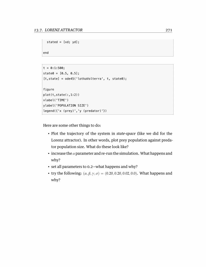
13.7. LORENZ ATTRACTOR 271
stated = [xd; yd];
end
t = 0:1:500;
state0 = [0.5, 0.5];
[t,state] = ode45('lotkaVolterra', t, state0);
figure
plot(t,state(:,1:2))
xlabel('TIME')
ylabel('POPULATION SIZE')
legend({'x (prey)','y (predator)'})
Here are some other things to do:
• Plot the trajectory of the system in state-space (like we did for theLorenz attractor). In other words, plot prey population against preda-tor population size. What do these look like?
• increase theαparameter and re-run the simulation. Whathappens andwhy?
• set all parameters to 0.2—what happens and why?• try the following: (α, β, γ, σ) = (0.20, 0.20, 0.02, 0.0). What happens and
why?

LINKS 272
Links
179http://en.wikipedia.org/wiki/Lotka_Volterra_equation
180http://en.wikipedia.org/wiki/Hodgkin-Huxley_model
181http://en.wikipedia.org/wiki/Hooke's_law
182http://en.wikipedia.org/wiki/Newton's_laws_of_motion
183http://en.wikipedia.org/wiki/Newton's_laws_of_motion#Newton.27s_second_law
184http://en.wikipedia.org/wiki/Runge–Kutta_methods
185http://en.wikipedia.org/wiki/Gravitational_constant
186https://en.wikipedia.org/wiki/Double_pendulum
187http://en.wikipedia.org/wiki/Lorenz_system
188http://en.wikipedia.org/wiki/Nonlinear_system
189http://en.wikipedia.org/wiki/Chaos_theory
190http://en.wikipedia.org/wiki/Butterfly_effect
191https://www.youtube.com/watch?v=YS_xtBMUrJg
192http://en.wikipedia.org/wiki/Damping

14 Modelling Action Potentials
In this chapter we will use a model of voltage-gated ion channels in a single neu-ron to simulate action potentials. The model is based on the work by Hodgkin &Huxley in the 1940s and 1950s. A good reference to refresh your memory abouthow ion channels in a neuron work is the Kandel, Schwartz & Jessel book “Prin-ciples of Neural Science”.
• A. L. Hodgkin and A. F. Huxley. A quantitative description of membranecurrent and its application to conduction and excitation in nerve. J. Physiol.(Lond.), 117(4):500-544, Aug 1952
• A. L. Hodgkin, A. F. Huxley, A. L. Hodgkin, and A. F. Huxley. A quantitativedescription of membrane current and its application to conduction and ex-citation in nerve. 1952. Bull. Math. Biol., 52(1-2):25-71, 1990
• O. Ekeberg, P. Wallen, A. Lansner, H. Traven, L. Brodin, and S. Grillner. Acomputer based model for realistic simulations of neural networks. I. Thesingle neuron and synaptic interaction. Biol Cybern, 65(2):81-90, 1991
• E.R. Kandel, J.H. Schwartz, T.M. Jessell, et al. Principles of neural science,volume 4. McGraw-Hill New York, 2000
To model the action potential we will use an article by Ekeberg et al. (1991) pub-lished in Biological Cybernetics (see citation above). When reading the articleyou can focus on the first three pages (up to paragraph 2.3) and try to find an-swers to the following questions:
273

14.1. THE NEURON MODEL 274
• How many differential equations are there?• What is the order of the system described in equations 1-9?• What are the states and state derivatives of the system?
Before we begin coding up the model, it may be useful to remind you of a funda-mental law of electricity, one that relates electrical potentialV to electric currentI and resistanceR (or conductanceG, the reciprocal of resistance). This of courseis known as Ohm’s law193:
V = IR (14.1)
or
V =IG (14.2)
Our goal here is to code up a dynamical model of the membrane’s electric circuitincluding two types of ion channels: sodium and potassium channels. We willuse thismodel tobetterunderstand theprocessunderlying theoriginof anactionpotential.
14.1 The Neuron Model
Figure 14.1 below, adapted from Ekeberg et al., 1991, schematically illustratesthemodel of a neuron. In panel Awe see a soma, andmultiple dendrites. Each ofthese can be modelled by an electrical “compartment” (Panel B) and the passiveinteractions between themcan bemodelled as a pretty standard electrical circuit(see Biological Neuron Model194 for more details about compartmental modelsof neurons). In panel C, we see an expanded model of the Soma from panel A.Here, a number of active ion channels are included in the model of the soma.

14.1. THE NEURON MODEL 275
Figure 14.1: Schematic of Ekeberg et al. 1991 neuron model
For our purposes here, we will focus on the soma, and we will not include anyadditional dendrites in our implementation of the model. Thus essentially wewill be modelling what appears in panel C, and at that, only a subset.
In panel C we see that the soma can be modelled as an electrical circuit with asodium ion channel (Na), a potassium ion channel (K), a calcium ion channel(Ca), and a calcium-dependent potassium channel (K(Ca)). What we will be con-cerned with simulating, ultimately, is the intracellular potential E.

14.2. PASSIVE PROPERTIES 276
14.2 Passive Properties
Equation (1) of Ekeberg is a differential equation describing the relation betweenthe time derivative of the membrane potential E as a function of the passive leakcurrent through the membrane, and the current through the ion channels. Notethat Ekeberg uses E instead of the typical V symbol to represent electrical poten-tial.
dEdt =
(Eleak − E)Gm +∑(Ecomp − E)Gcore + Ichannels
Cm(14.3)
Don’t panic, it’s not actually that complicated. What this equation is saying isthat the rate of change of electrical potential across the current (the left handside of the equation, dE
dt ) is equal to the sum of a bunch of other terms, dividedby membrane capacitance Cm (the right hand side of the equation). Recall frombasic physics that capacitance195 is a measure of the ability of something to storean electrical charge.
The “bunch of other things” is a sum of three things, actually, (from left to right):a passive leakage current, plus a term characterizing the electrical coupling ofdifferent compartments, plus the currents of the various ion channels. Since weare not going to be modelling dendrites here, we can ignore the middle term onthe right hand side of the equation
∑(Ecomp − E)Gcore which represents the sumof currents from adjacent compartments (we have none).
We are also going to include in our model an external current Iext. This can es-sentially represent the sum of currents coming in from the dendrites (which weare not explicitly modelling). It can also represent external current injected in apatch-clamp196 experiment. This is what we as experimenters can manipulate,for example, to see how neuron spiking behaviour changes. So what we will ac-tually be working with is this:

14.3. SODIUM CHANNELS (NA) 277
dEdt =
(Eleak − E)Gm + Ichannels + IextCm
(14.4)
Whatweneed todonow isunpack the Ichannels termrepresenting the currents fromall of the ion channels in the model. Initially we will only be including two, thepotassium channel (K) and the sodium channel (Na).
14.3 Sodium Channels (Na)
The current through sodium channels that enter the soma are represented byequation (2) in Ekeberg et al. (1991):
INa = (ENa − Esoma)GNam3h (14.5)
where m is the activation of the sodium channel and h is the inactivation of thesodium channel, and the other terms are constant parameters: ENa is the rever-sal potential,GNa is the maximum sodium conductance throught the membrane,and Esoma is the membrane potential of the soma.
The activationm of the sodium channels is described by the differential equation(3) in Ekeberg et al. (1991):
dmdt = αm(1−m)− βmm (14.6)
where αm represents the rate at which the channel switches from a closed to anopen state, and βm is rate for the reverse. These two parameters α and β dependon the membrane potential in the soma. In other words the sodium channel isvoltage-gated. Equation (4) in Ekeberg et al. (1991) gives these relationships:
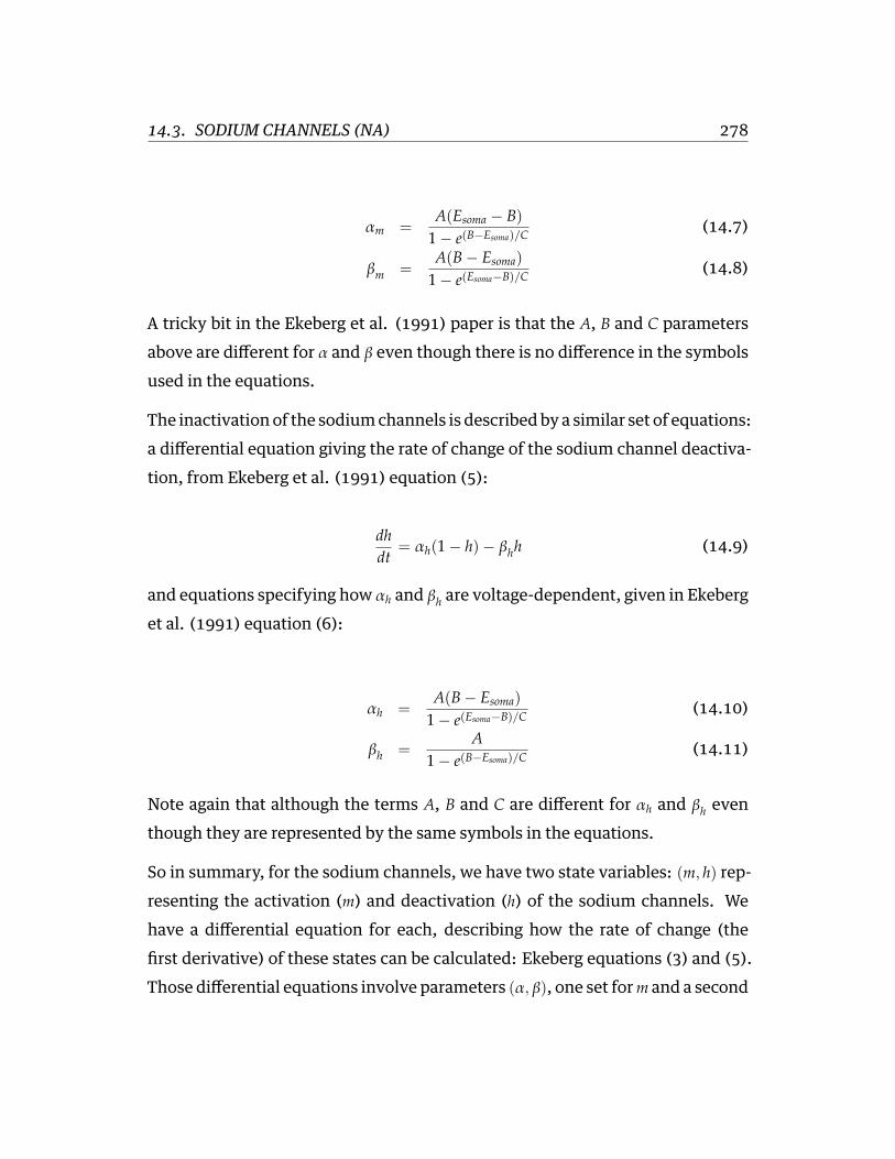
14.3. SODIUM CHANNELS (NA) 278
αm =A(Esoma − B)1− e(B−Esoma)/C (14.7)
βm =A(B− Esoma)1− e(Esoma−B)/C (14.8)
A tricky bit in the Ekeberg et al. (1991) paper is that the A, B and C parametersabove are different for α and β even though there is no difference in the symbolsused in the equations.
The inactivationof the sodiumchannels is describedby a similar set of equations:a differential equation giving the rate of change of the sodium channel deactiva-tion, from Ekeberg et al. (1991) equation (5):
dhdt = αh(1− h)− βhh (14.9)
and equations specifying how αh and βh are voltage-dependent, given in Ekeberget al. (1991) equation (6):
αh =A(B− Esoma)1− e(Esoma−B)/C (14.10)
βh =A
1− e(B−Esoma)/C (14.11)
Note again that although the terms A, B and C are different for αh and βh eventhough they are represented by the same symbols in the equations.
So in summary, for the sodium channels, we have two state variables: (m, h) rep-resenting the activation (m) and deactivation (h) of the sodium channels. Wehave a differential equation for each, describing how the rate of change (thefirst derivative) of these states can be calculated: Ekeberg equations (3) and (5).Those differential equations involve parameters (α, β), one set form and a second

14.4. POTASSIUM CHANNELS (K) 279
set for h. Those (α, β) parameters are computed from Ekeberg equations (4) (form) and (6) (for h). Those equations involve parameters (A,B,C) that have param-eter values specific to α and β andm and h (see Table 1 of Ekeberg et al., 1991).
14.4 Potassium Channels (K)
The potassium channels are represented in a similar way, although in this casethere is only channel activation, and no inactivation. In Ekeberg et al. (1991)the three equations (7), (8) and (9) represent the potassium channels:
Ik = (Ek − Esoma)Gkn4 (14.12)
dndt = αn(1− n)− βnn (14.13)
where n is the state variable representing the activation of potassium channels.As before we have expressions for (α, β) which represent the fact that the potas-sium channel is also voltage-gated:
αn =A(Esoma − B)1− e(B−Esoma)/C (14.14)
βn =A(B− Esoma)1− e(Esoma−B)/C (14.15)
Again, the parameter values for (A,B,C) can be found in Ekeberg et al., (1991)Table 1.
To summarize, the potassium channel has a single state variable n representingthe activation of the potassium channel.

14.5. SUMMARY 280
14.5 Summary
We have a model now that includes four state variables:
1. E representing the potential in the soma, given by differential equation (1)in Ekeberg et al., (1991)
2. m representing the activation of sodium channels, Ekeberg equation (3)3. h representing the inactivation of sodium channels, Ekeberg equation (5)4. n representing the activation of potassium channels, Ekeberg equation (8)
Each of the differential equations that define how to compute state derivatives,involve (α, β) terms that are given by Ekeberg equations (4) (form), (6) (for h) and(9) (for n).
So what we have to do in order to simulate the dynamic behaviour of this neu-ron over time, is simply to implement these equations in MATLAB code, give thesystem some reasonable initial conditions, and simulate it over time using theode45() function.
14.6 MATLAB code
Here is a MATLAB function called ekeberg.m that implements the equations. Itlooks intimidating but really it’s just an implementation of the equations above.
function stated = ekeberg(t,state,params)
% Purpose: simulate Hodgkin and Huxley model for the action potential using
% the equations from Ekeberg et al, Biol Cyb, 1991
% Input: state ([E m h n] (ie [membrane potential; activation of
% Na++ channel; inactivation of Na++ channel; activation of K+
% channel]),
% t (time),
% and the params (parameters of neuron; see Ekeberg et al)
% Output: statep (state derivatives)

14.6. MATLAB CODE 281
E = state(1);
m = state(2);
h = state(3);
n = state(4);
Epar = params.E;
Na = params.Na;
K = params.K;
% external current (from "voltage clamp", other compartments, other
% neurons, etc)
I_ext = Epar.I_ext;
% calculate Na rate functions and I_Na
alpha_act = Na.A_alpha_m_act * (E-Na.B_alpha_m_act) / ...
(1.0 - exp((Na.B_alpha_m_act-E) / Na.C_alpha_m_act));
beta_act = Na.A_beta_m_act * (Na.B_beta_m_act-E) / ...
(1.0 - exp((E-Na.B_beta_m_act) / Na.C_beta_m_act) );
dmdt = ( alpha_act * (1.0 - m) ) - ( beta_act * m );
alpha_inact = Na.A_alpha_m_inact * (Na.B_alpha_m_inact-E) / ...
(1.0 - exp((E-Na.B_alpha_m_inact) / Na.C_alpha_m_inact));
beta_inact = Na.A_beta_m_inact / (1.0 + (exp((Na.B_beta_m_inact-E) / ...
Na.C_beta_m_inact)));
dhdt = ( alpha_inact*(1.0 - h) ) - ( beta_inact*h );
% Na-current:
I_Na =(Na.Na_E-E) * Na.Na_G * (m^Na.k_Na_act) * h;
% calculate K rate functions and I_K
alpha_kal = K.A_alpha_m_act * (E-K.B_alpha_m_act) / ...
(1.0 - exp((K.B_alpha_m_act-E) / K.C_alpha_m_act));
beta_kal = K.A_beta_m_act * (K.B_beta_m_act-E) / ...
(1.0 - exp((E-K.B_beta_m_act) / K.C_beta_m_act));

14.6. MATLAB CODE 282
dndt = ( alpha_kal*(1.0 - n) ) - ( beta_kal*n );
I_K = (K.k_E-E) * K.k_G * n^K.k_K;
% leak current
I_leak = (Epar.E_leak-E) * Epar.G_leak;
% calculate derivative of E
dEdt = (I_leak + I_K + I_Na + I_ext) / Epar.C_m;
stated = [dEdt; dmdt; dhdt; dndt];
end
Here is a MATLAB script called go_ekeberg.m that sets up the parameters of themodel, and runs a simulation:
%% setup parameters
E.E_leak = -7.0e-2;
E.G_leak = 3.0e-09;
E.C_m = 3.0e-11;
E.I_ext = 0*1.0e-10;
Na.Na_E = 5.0e-2;
Na.Na_G = 1.0e-6;
Na.k_Na_act = 3.0e+0;
Na.A_alpha_m_act = 2.0e+5;
Na.B_alpha_m_act = -4.0e-2;
Na.C_alpha_m_act = 1.0e-3;
Na.A_beta_m_act = 6.0e+4;
Na.B_beta_m_act = -4.9e-2;
Na.C_beta_m_act = 2.0e-2;
Na.l_Na_inact = 1.0e+0;
Na.A_alpha_m_inact = 8.0e+4;
Na.B_alpha_m_inact = -4.0e-2;

14.6. MATLAB CODE 283
Na.C_alpha_m_inact = 1.0e-3;
Na.A_beta_m_inact = 4.0e+2;
Na.B_beta_m_inact = -3.6e-2;
Na.C_beta_m_inact = 2.0e-3;
K.k_E = -9.0e-2;
K.k_G = 2.0e-7;
K.k_K = 4.0e+0;
K.A_alpha_m_act = 2.0e+4;
K.B_alpha_m_act = -3.1e-2;
K.C_alpha_m_act = 8.0e-4;
K.A_beta_m_act = 5.0e+3;
K.B_beta_m_act = -2.8e-2;
K.C_beta_m_act = 4.0e-4;
params.E = E;
params.Na = Na;
params.K = K;
%% simulate
% set initial states and time vector
state0 = [-70e-03, 0, 1, 0];
t = 0:0.001:0.2;
% let's inject some external current
params.E.I_ext = 1.0e-10;
% run simulation
ekeberg_f = @(t,state) ekeberg(t,state,params);
[t,state] = ode45(ekeberg_f, t, state0);
%% plot the results
figure('position',[39 268 560 925],'paperposition',[2.4 2.5 3.6 6.0])

14.6. MATLAB CODE 284
subplot(4,1,1)
plot(t, state(:,1))
title('membrane potential')
subplot(4,1,2)
plot(t, state(:,2))
title('Na2+ channel activation')
subplot(4,1,3)
plot(t, state(:,3))
title('Na2+ channel inactivation')
subplot(4,1,4)
plot(t, state(:,4))
title('K+ channel activation')
xlabel('TIME (sec)')
What you will see is a figure as shown in Figure 14.2 below.

14.6. MATLAB CODE 285
Exercises
E 14.1 Alter the code so that themodelled neurononly has the leakage current andexternal current. In other words, comment out the terms related to sodiumand potassium channels. Run a simulation with an initial membrane poten-tial of -70mv and an external current of 0.0mv. What happens and why?
E 14.2 Change the external current to 1.0e-10 and re-run the simulation. Whathappens and why?
E 14.3 Add in the terms related to the sodium channel (activation and deactiva-tion). Run a simulation with external current of 1.0e-10 and initial states[-70e-03, 0, 1]. What happens and why?
E 14.4 Add in the terms related to the potassium channel. Run a simulation withexternal current of 1.0e-10 and initial states [-70e-03, 0, 1, 0]. What hap-pens and why?
E 14.5 Play with the external current level (increase it slightly, decrease it slightly,etc). What is the effect on the behaviour of the neuron?
E 14.6 What is the minimum amount of external current necessary to generate anaction potential? Why?

LINKS 286
Links
193http://en.wikipedia.org/wiki/Ohm's_law
194http://en.wikipedia.org/wiki/Biological_neuron_model
195http://en.wikipedia.org/wiki/Capacitance
196http://en.wikipedia.org/wiki/Patch_clamp

LINKS 287
Figure 14.2: Simulation of a neuron using equations from Ekeberg et al., Biol. Cybern.(1991)

LINKS 288

15 Basic statistical tests
MATLAB has a toolbox called the Statistics and Machine Learning Toolbox thatcontains many, many useful functions for statistical analyses.
Statistics and Machine Learning Toolbox197 documentation.
We will review only a small subset of its functionality here, so you can get a feelfor how you might analyse data in MATLAB.
15.1 Probability Distributions
MATLAB has support for a number of common probability distributions includ-ing discrete and continuous distributions, including (but not limited to) the fol-lowing:
• Uniform• Normal (Gaussian)• Binomial• Poisson• Beta• Chi-Square• Exponential• Gamma• Lognormal• Student’s t
289

15.1. PROBABILITY DISTRIBUTIONS 290
• Weibull• F distribution
Each distribution will have functions in MATLAB for the following:
• cumulative distribution function• probability density function• inverse cumulative distribution function• generating random values
So for example for a Normal distribution with mean 100 and standard deviation15, you could find the area under the curve to the left of the value x=130 using:
y = cdf('Normal',130,100,15)
y =
0.9772
This tells you that 130 is the 97.72 percentile.
To generate random values using a Normal distribution you could use either therandom function or the more direct randn function. To generate 10 random valuesfrom a Normal distribution with mean 100 and standard deviation 15:
y = randn(1,10)*15 + 100
y =
108.0650 127.5083 66.1173 112.9326 104.7815 80.3847 93.4961 105.
1394 153.6760 141.5416
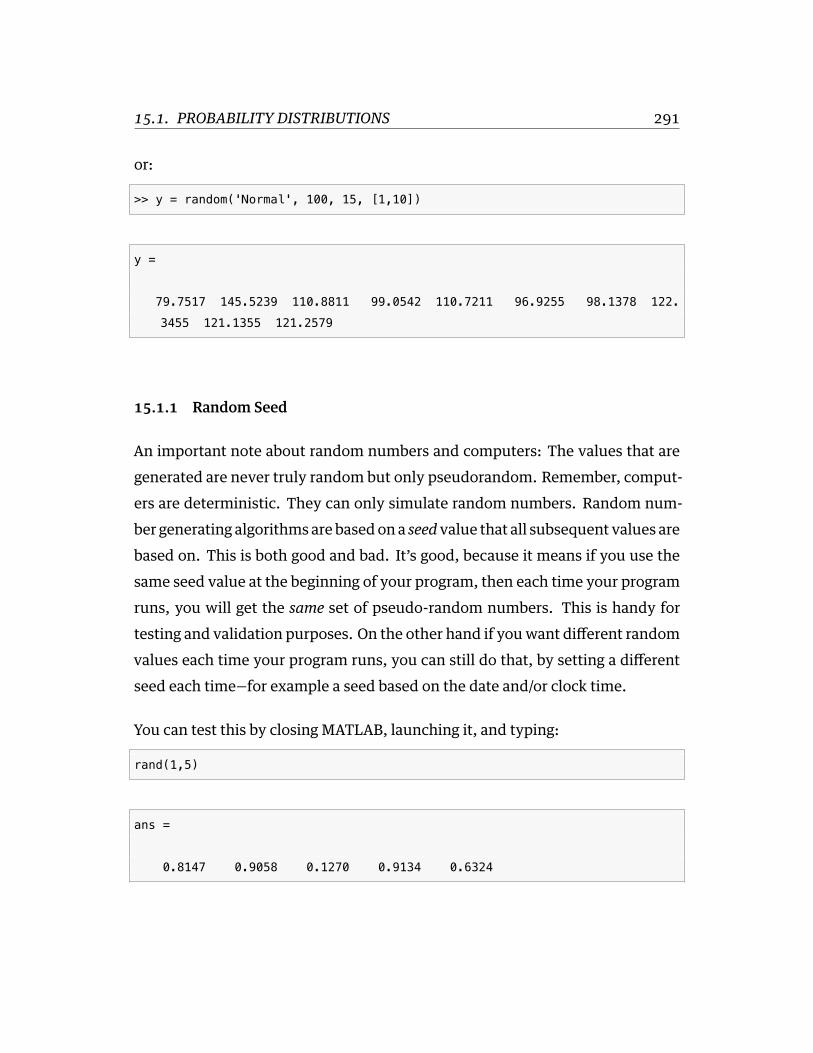
15.1. PROBABILITY DISTRIBUTIONS 291
or:
>> y = random('Normal', 100, 15, [1,10])
y =
79.7517 145.5239 110.8811 99.0542 110.7211 96.9255 98.1378 122.
3455 121.1355 121.2579
15.1.1 Random Seed
An important note about random numbers and computers: The values that aregenerated are never truly random but only pseudorandom. Remember, comput-ers are deterministic. They can only simulate random numbers. Random num-ber generating algorithms are basedon a seedvalue that all subsequent values arebased on. This is both good and bad. It’s good, because it means if you use thesame seed value at the beginning of your program, then each time your programruns, you will get the same set of pseudo-random numbers. This is handy fortesting and validation purposes. On the other hand if you want different randomvalues each time your program runs, you can still do that, by setting a differentseed each time—for example a seed based on the date and/or clock time.
You can test this by closing MATLAB, launching it, and typing:
rand(1,5)
ans =
0.8147 0.9058 0.1270 0.9134 0.6324

15.1. PROBABILITY DISTRIBUTIONS 292
Now close MATLAB again and re-open it again, and re-type:
rand(1,5)
and you ought to get the same random values:
ans =
0.8147 0.9058 0.1270 0.9134 0.6324
To set the random seed in MATLAB to a different value, put this line of code atthe beginning of your program:
rng('shuffle')
rand(1,5)
ans =
0.3672 0.7020 0.8560 0.0797 0.5879
15.1.2 Fitting
MATLABhas a function called fitdist thatwill fit a givenprobability distributionto some data. Here is how to use it. First let’s generate 100 data points from aNormal distribution with mean 0 and standard deviation 1:
fitdist
x = randn(100,1);

15.2. HYPOTHESIS TESTS 293
Now let’s use fitdist to fit the (2) parameters of aNormal distribution (meanmu,and standard deviation sigma) to the data:
d = fitdist(x, 'normal');
produces:
d =
NormalDistribution
Normal distribution
mu = -0.0726815 [-0.272105, 0.126743]
sigma = 1.00505 [0.882442, 1.16754]
You can use fitdist with other distributions besides Normal, just see the docu-mentation in MATLAB.
15.2 Hypothesis Tests
MATLAB has functionality for various kinds of statistical hypothesis tests. Herewe outline just a few. See the full documentation for all the details.
15.2.1 t-test
The function ttest performs a one-sample or a paired-sample t-test. The func-tion ttest2 performs an independent samples t-test.
Imagine we have a dependent variable measured from 5 subjects in two condi-tions:
c1 = [1,3,2,3,3];
c2 = [2,5,4,3,5];

15.2. HYPOTHESIS TESTS 294
We can perform a paired-samples t-test:
[H,P,CI,STATS] = ttest(c1,c2)
H =
1
P =
0.0249
CI =
-2.5106 -0.2894
STATS =
tstat: -3.5000
df: 4
sd: 0.8944
The first parameter is whether we reject (1=TRUE) or not (0=FALSE) the null hy-pothesis that the two groups were sampled from the same population. The sec-ondparameter gives theprobability of obtaining a valueof t as large as theonewedid, under the null hypothesis. In this case, p=0.0249. The third parameter is anarray containing the 95% confidence interval on the difference between means.The fourthparameter is a structwith the t-statistic, thedegrees of freedomof thet-test, and the estimate of the standard error of the differences between means.

15.2. HYPOTHESIS TESTS 295
You might report the result of this t-test in a paper like this: t(4)=-3.5, p=0.0249.
There are optional parameters to pass to the ttest function for things like one-tailed vs two-tailed tests, and alpha level for rejecting the null hypothesis.
Also have a look at ttest2 for independent-samples t-tests. Here you also have asan optional parameter whether to assume equal or unequal variances.
15.2.2 Analysis of Variance
MATLAB has a number of functions for performing different kinds of analyses ofvariance:
• anova1: One-way analysis of variance• anova2: Two-way analysis of variance• anovan: N-way analysis of variance• aoctool: Analysis of Covariance• ANOVA with Random Effects198
• ranova: Repeated-Measures ANOVA• manova: Multivariate analysis of variance
We are not going to go through all the different kinds of ANOVA here. For nowlet’s just see a simple example of a two-factor, between-subjects ANOVA.
MATLAB includes sample data from a study of popcorn brands and popper types.The columns are brands: (Gourmet, National, Generic) and the rows are poppertypes (Oil vs Air). The dependent variable is the yield of popped popocorn, mea-sured in cups. The first 3 rows are the oil popper and the last 3 rows are the airpopper. Researchers popped a batch of each brand three times with each popper,i.e. the number of replications in each cell of the design is 3.
load popcorn
popcorn

15.2. HYPOTHESIS TESTS 296
popcorn =
5.5000 4.5000 3.5000
5.5000 4.5000 4.0000
6.0000 4.0000 3.0000
6.5000 5.0000 4.0000
7.0000 5.5000 5.0000
7.0000 5.0000 4.5000
To perform a two-way ANOVA and save the output into a cell array called tbl:
[p,tbl] = anova2(popcorn, 3);
Source SS df MS F Prob>F
----------------------------------------------------
Columns 15.75 2 7.875 56.7 0
Rows 4.5 1 4.5 32.4 0.0001
Interaction 0.0833 2 0.04167 0.3 0.7462
Error 1.6667 12 0.13889
Total 22 17
We get a standard ANOVA table output in a Figure window. We also have thesevalues in our tbl variable:
>> tbl
tbl =
'Source' 'SS' 'df' 'MS' 'F' 'Prob>F'
'Columns' [15.7500] [ 2] [7.8750] [56.7000] [7.6790e
-07]
'Rows' [ 4.5000] [ 1] [4.5000] [32.4000] [1.0037e

15.2. HYPOTHESIS TESTS 297
-04]
'Interaction' [ 0.0833] [ 2] [0.0417] [ 0.3000] [ 0.
7462]
'Error' [ 1.6667] [12] [0.1389] []
[]
'Total' [ 22] [17] [] []
[]
So we see there is a significant main effect of Columns (popper Brand,F(2,12)=56.7, p<.0000001), a significant main effect of Rows (popper type,F(1,12)=32.4, p<.0001) and no significant interaction effect (F(2,12)=0.3,p>.7462).
See the documentation for multcompare to see how to run post-hoc multiple com-parisons on the data, to see which groups are reliably different.
15.2.3 Multiple Regression
MATLAB comes with a sample dataset called carsmall, which contains all sortsof measures of 100 automobiles including:
• acceleration• number of engine cylinders• engine displacement• engine horsepower• manufacturer• model• model year• miles per gallon• origin• weight

15.2. HYPOTHESIS TESTS 298
Let’s say we want to produce a multiple regression model that uses Weight andAcceleration to predict Miles Per Gallon. First store our data in a table:
tbl = table(Weight,Acceleration,MPG,'VariableNames',{'Weight','Acceleration
','MPG'});
We can then use fitlm to fit a linear regression model to the data:
lm = fitlm(tbl, 'MPG ~ Weight + Acceleration')
This says, make a linear model where the MPG variable depends on ( ) Weightand Acceleration.
The regression equation looks like this:
MPG = β0 + β1Weight+ β2Acceleration (15.1)
lm =
Linear regression model:
MPG ~ 1 + Weight + Acceleration
Estimated Coefficients:
Estimate SE tStat pValue
__________ __________ _______ __________
(Intercept) 45.155 3.4659 13.028 1.6266e-22
Weight -0.0082475 0.00059836 -13.783 5.3165e-24
Acceleration 0.19694 0.14743 1.3359 0.18493
Number of observations: 94, Error degrees of freedom: 91
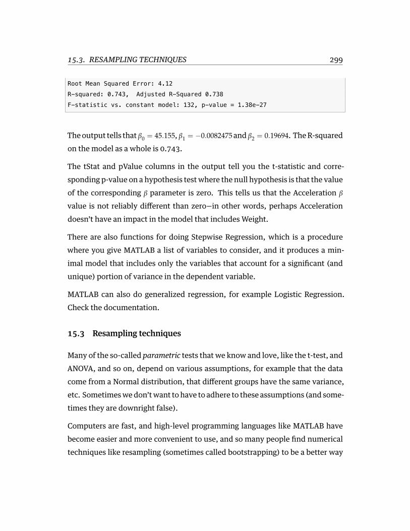
15.3. RESAMPLING TECHNIQUES 299
Root Mean Squared Error: 4.12
R-squared: 0.743, Adjusted R-Squared 0.738
F-statistic vs. constant model: 132, p-value = 1.38e-27
Theoutput tells that β0 = 45.155, β1 = −0.0082475 and β2 = 0.19694. TheR-squaredon the model as a whole is 0.743.
The tStat and pValue columns in the output tell you the t-statistic and corre-sponding p-value on a hypothesis testwhere the null hypothesis is that the valueof the corresponding β parameter is zero. This tells us that the Acceleration βvalue is not reliably different than zero—in other words, perhaps Accelerationdoesn’t have an impact in the model that includes Weight.
There are also functions for doing Stepwise Regression, which is a procedurewhere you give MATLAB a list of variables to consider, and it produces a min-imal model that includes only the variables that account for a significant (andunique) portion of variance in the dependent variable.
MATLAB can also do generalized regression, for example Logistic Regression.Check the documentation.
15.3 Resampling techniques
Many of the so-called parametric tests that we know and love, like the t-test, andANOVA, and so on, depend on various assumptions, for example that the datacome from a Normal distribution, that different groups have the same variance,etc. Sometimeswedon’twant tohave to adhere to these assumptions (and some-times they are downright false).
Computers are fast, and high-level programming languages like MATLAB havebecome easier and more convenient to use, and so many people find numericaltechniques like resampling (sometimes called bootstrapping) to be a better way

15.3. RESAMPLING TECHNIQUES 300
to go.
Let’sproceedusinganexample inwhichwehave twogroups: a control groupanda drug group. Each group has 10 (different) subjects. Each subject contributesone score. Here are the data:
g1 = [3,2,2,4,2,1,2,3,3,2]';
g2 = [4,3,3,2,3,5,4,3,6,4]';
We could do an independent-samples t-test on the data like this:
[h,p,ci,stats] = ttest2(g1,g2)
h =
1
p =
0.0102
ci =
-2.2525 -0.3475
stats =
tstat: -2.8673
df: 18
sd: 1.0138

15.3. RESAMPLING TECHNIQUES 301
And we see we get a p-value of 0.0102. But let’s say we don’t want to have tomake the assumptions that the population data are Normal and the variances areequal. Let’s instead do a bootstrap/resampling test.
The idea here is to simulate the null hypothesis, namely that both groups are sam-pled from the same population. Now we don’t have access to the stimulated pop-ulation, all we have are these two samples. What we will do then, is throw bothsamples into a bucket, and pretend that is our stipulated single population. Wewill then simulate sampling from that bucket, with replacement, to reconstitutetwo groups. We will then compute a statistic of interest on those two groups (forexample, thedifferencebetweenmeans). Wewill then repeat this a largenumberof time (e.g. 5000) and count how many times we obtained a difference betweenmeans as large as the one in the real data. If that turns out to be sufficiently rare,we can reject the null hypothesis.
We can use the datasample function in MATLAB to accomplish this. The functionwill re-sample a list of numbers, with replacement. We simply imbed this in aloop and afterwards, compute our statistic of interest—in this case, thedifferencebetween means (but it could be anything you want).
% shuffle the random number generator seed
%
rng('shuffle')
N = 5000;
g_all = [g1;g2]; % throw both groups into a bucket
% pre-allocate an array to store our statistic of interest
% and loop N times, each time simulating the null hypothesis
% namely, sampling with replacement from the bucket to
% reconstitute the two groups, then re-computing the
% statistic of interest (the difference between means)
%

15.3. RESAMPLING TECHNIQUES 302
boot = ones(N,1);
for i=1:N
g_resamp = datasample(g_all, 20);
boot(i) = mean(g_resamp(1:10)) - mean(g_resamp(11:20));
end
We get an array boot which contains our statistic of interest for each of the 5000boostrap runs. We can use the boot array to ask the question, how many timesout of the 5000 bootstrap runs didweobtain a difference betweenmeans as largeas the one for our actual observed data?
% compute actual observed difference between means
%
dm_observed = mean(g1) - mean(g2);
disp(sprintf('actual dm = %.3f', dm_observed))
% how many times in the bootstrap did we get a
% difference between means as large (far from zero)?
%
n_big = length( find( boot <= dm_observed ) );
disp(sprintf('%d times out of %d was dm as extreme as %.3f', ...
n_big, N, dm_observed))
actual dm = -1.300
33 times out of 5000 was dm as extreme as -1.300
When I ran this I got 33 times out of 5000 was the boostrapped value as extremeas the empirically observed one. You might get something slightly different ifyour random number generator was seeded using a different value.
We can draw a histogram of the boostrapped distribution of differences betweenmeans, and overlay using a vertical red line, our empirically observed difference

15.3. RESAMPLING TECHNIQUES 303
between means:
hist(boot)
hold on
plot([dm_observed dm_observed], get(gca,'ylim'), 'r-', 'linewidth',2)
You will see something like what is shown in Figure 15.1 below.
-2 -1.5 -1 -0.5 0 0.5 1 1.5 20
200
400
600
800
1000
1200
1400
Figure 15.1: Boostrapped distribution of difference between means.
Of the 5000 simulations of the null hypothesis, it’s relatively rare that we get adifference between means as extreme as the empirically observed value (the redvertical line). Most of the time, we get a difference between means near zero.This makes sense under the null hypothesis.
Specifically then, 33 times out of 5000 we obtained a difference between meansas extreme as our empirically observed value. This corresponds to p=33/5000which is 0.0066 (or 0.01 rounded up), about the same as the t-test p-value above.Here though we didn’t have to make any assumptions about the underlying dis-tribution, or variances, or anything like that.

15.3. RESAMPLING TECHNIQUES 304
If we adopt an alpha level of p=0.05, then our observed p=0.01 might cause usto reject the null hypothesis that the two groups were sampled from the samepopulation.
This approach can be used for just about any statistical test. Some people saythat since computers are fast, we might as well do statistical tests this way, sincewe don’t have to make assumptions.
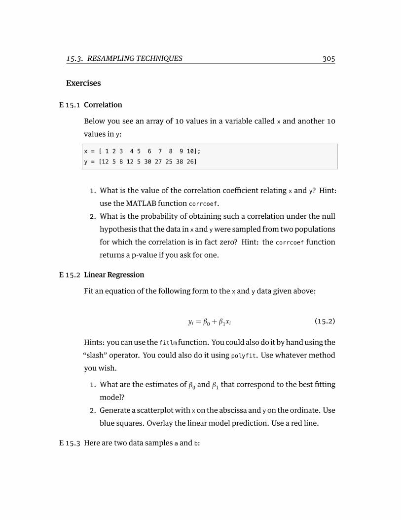
15.3. RESAMPLING TECHNIQUES 305
Exercises
E 15.1 Correlation
Below you see an array of 10 values in a variable called x and another 10values in y:
x = [ 1 2 3 4 5 6 7 8 9 10];
y = [12 5 8 12 5 30 27 25 38 26]
1. What is the value of the correlation coefficient relating x and y? Hint:use the MATLAB function corrcoef.
2. What is the probability of obtaining such a correlation under the nullhypothesis that the data in x and ywere sampled from twopopulationsfor which the correlation is in fact zero? Hint: the corrcoef functionreturns a p-value if you ask for one.
E 15.2 Linear Regression
Fit an equation of the following form to the x and y data given above:
yi = β0 + β1xi (15.2)
Hints: you canuse the fitlm function. Youcould alsodo it byhandusing the“slash” operator. You could also do it using polyfit. Use whatever methodyou wish.
1. What are the estimates of β0 and β1 that correspond to the best fittingmodel?
2. Generate a scatterplotwith x on the abscissa and y on the ordinate. Useblue squares. Overlay the linear model prediction. Use a red line.
E 15.3 Here are two data samples a and b:

15.3. RESAMPLING TECHNIQUES 306
a = [2 6 6 1 1 4 9 3 5 2];
b = [6 8 9 5 9 12 4 5 4 7];
Using resampling, test the hypothesis that the two samples were drawnfrom populations with the same mean. Use n=10,000 iterations.
• How many times out of 10,000 do you get a difference between meansas extreme as the one observed between a and b?
• What is the corresponding p-value?• What would be the difference between means that corresponds to ap = 0.05 level of significance?

LINKS 307
Links
197http://www.mathworks.com/help/stats/
198http://www.mathworks.com/examples/statistics/2176-anova-with-random-effects