Embed Size (px)
Citation preview

V.A. Solé NSLS-II 21/04/2010
Scientific Computing at the ESRFV.A. Solé
ESRF Data Analysis

V.A. Solé NSLS-II 21/04/2010
Outline
• Data handling requirements for high-data-rate experiments• Experimental data storage policies• Data reduction and analysis capabilities during user
experiments• Post-experiment data analysis support and accessibility• Organization structure (optimized?) to achieve the goals
“We would like speakers to highlight specifically the lessons learned, good and bad.”

V.A. Solé NSLS-II 21/04/2010
High data rate experiments
Tomography beamlines: id19, id17, id15 and (partially) id22

V.A. Solé NSLS-II 21/04/2010
High Data Rate Experiments: ID15• Experiment:
• Absorption and phase contrast tomography• Detector:
• 2k x 2k pixel 16 bit CMOS PCO camera• Camera supported data rate:
• > 1000 full frame images/s – > 8 Gbytes/second• 106 binned images/s Potentially a full tomography in less than 1s
• Bottleneck:• Data transfer and storage (current limitation) • Data analysis (if previous issue solved)
• Data access:• Most users come with their own disks to take data with them• Data analysis often performed on site

V.A. Solé NSLS-II 21/04/2010
ID17 & ID19: The Malapa hominid study

V.A. Solé NSLS-II 21/04/2010
The Malapa hominid study
Multiscale analysis performed on ID17 and ID19 in February 2010
Around 10 TB of basic data (radiographs)
Around 15 additional terabytes of data after processing
1 full month of calculation for reconstruction and artifact corrections with 100 processors, using at least 7 steps of processing.
Probably 1-2 years of analysis before having the first important results on dental development and internal anatomy
Acknowledgements : Paul Tafforeau, ESRF

V.A. Solé NSLS-II 21/04/2010
Data storage lessons
• We all know writing can be a limiting factor on acquisition• READING can be a limiting factor on analysis!
• Data readout from our central filesystem can be as slow as 20 Mb/s• A simple ‘ls’ on directories with thousands of files takes minutes
(provider answer: price to pay for massive cluster structure)
“First test and then buy” approach

V.A. Solé NSLS-II 21/04/2010
ID22 – Fluorescence-Diffraction Tomography
DiffractionCCD
Sample
1cm
zx
y
�

V.A. Solé NSLS-II 21/04/2010
Ny��N�Diffraction Images
1cm
y
�
Sum Sinogram
Sum Pattern
Azimuthal Integrations
Ny�N� Diffraction Patterns
Fit2d software
Phase Sinograms
�y
PyMcasoftware
ReconstructionCapillaryCalcite
Ferrite
Cubicsp3
25�my
x
Acknowledgements: Pierre Bleuet CEA - Grenoble

V.A. Solé NSLS-II 21/04/2010
• Currently• Diffraction images in EDF or MarCCD format• Fluorescence data in EDF or SPEC file format• Scan information in SPEC file format• Result of azimutal integration on Fit2D .chi format
• Preparing to move to HDF5
Data format issues
Lesson learned: Try to avoid inventing a new data format. Use an existing one
Lesson NOT learned (yet?): Forget about ASCII just because you want to look at the file

V.A. Solé NSLS-II 21/04/2010
Experimental data storage policies• Before (-2009):
• Short term:• User account and data kept 30 days• In-house data kept 100 days
• Long term:• Additional ESRF 6 month backup
• Current (2009-):• Short term (800 Tb available, 150 Tb used, 1600 Tb foreseen):
• User account and data kept 30 days• User can request additional 30 days via web interface• In-house data older than one year deleted in June or December
• Long term:• Additional ESRF 6 month backup • 1 Tb/tape, currently 2150 tapes (max: ~ 8 Pb)

V.A. Solé NSLS-II 21/04/2010
Data reduction and analysis during user experiment• Beamline Staff applications:
• SPD (SAXS - Mainly ID02, several authors)• 2D spatial distortion correction, azimuthal integration, …
• X-ray Photon Correlation Spectroscopy (ID10 – Mainly Yuriy Chushkin)• ….
• Software Group applications:• Fit2D Diffraction. Andrew Hammersley• PyHST Tomographic reconstruction. Alessandro Mirone• PyMca X-Ray Fluorescence and Mapping. V. Armando Solé• XOP XAS, PD data reduction. Manuel Sánchez del Río
• EDNA Framework:• International collaboration• Linking together different codes

V.A. Solé NSLS-II 21/04/2010
Post-experiment data analysis support and access
• Protein crystallography • ISPyB Database• No remote analysis
• Tomography• TomoDB database with metadata and processed data• Raw data discarded after six months
• Others• Ready to use data analysis codes (Fit2D, PyMca, XOP, …)• Code repository from external collaborators• Availability of source code

V.A. Solé NSLS-II 21/04/2010
Organization to achieve the goals
• Data storage: PANData• Software project management• Programs and source code distribution
• Internally• Externally
• Faster processing• Parallel computing:
• MPI• Batch processing: Condor clusters
• Better hardware use:• Use GPUs
• Multivariate analysis• Workflow automation : EDNA

V.A. Solé NSLS-II 21/04/2010
PANData?
• Photon and Neutron Data Infrastructure• http://www.pan-data.net/Main_Page
• Aims• provide user communities with data repositories and data
management tools to • deal with large sets and data rates from the experiments,• enable easy and standardized annotation of data, • allow transparent and secure remote access to data, • establish sustainable and compatible data catalogues, • allow long-term preservation of data, and .
• provide compatible open source data analysis software
Proposal recently approved by the European Union

V.A. Solé NSLS-II 21/04/2010
Software Project Management
• Previous policy• Need driven
• Close developer-customer interaction• Not well-defined goals• Subjective priorities• No man-power cost estimation
• Current policy (just starting)• Project driven
• Well defined goals• Priorities set by management • Man-power costs estimation• Potentially weaker developer-customer interaction

V.A. Solé NSLS-II 21/04/2010
Programs and Source Code distribution
• Internally• via Bliss Installer and Bliss Builder (RPM based)
• Externally (Do not be paranoid about security!)• Tango repository in sourceforge• PyMca repository in sourceforge• BLISS tools at http://blissgarden.org• EDNA at http://www.edna-site.org• Inventory of scientific programs at:
http://www.esrf.eu/UsersAndScience/Experiments/TBS/SciSoft
• Current policy (joint ESRF – ILL site):http://forge.epn-campus.eu

V.A. Solé NSLS-II 21/04/2010
Batch Processing: Condor
Test job run time [s]Acknowledgements : Gabriele Förstner, ESRF, Max Nanao, EMBL
Num
ber of runs
42 hosts (166 cores), interactive and batch use

V.A. Solé NSLS-II 21/04/2010
Batch Processing: Condor policy
• Current implementation leads to unpredictable processing times
• Suggested policy• Clearly separated clusters for batch processing and for interactive work
• Considering• Different clusters and/or queues based of expected CPU time use
• The idea is to give priority to “fast” processes• A process not respecting the directives shall be automatically killed

V.A. Solé NSLS-II 21/04/2010
GPU: Gain in performances
Pre-processing backprojection0
5
10
15
20
25
SLICE 2048X2048
PyHSTPyHST_GPU
Tim
e ( s
econ
ds)
• Backprojection using GPU : • PyHST Performance• 2k x 2x pixels per image• 1 Slice = 2k x 2k images• Single precision calculation• 2 GPU Tesla C1060
• 240 processor/GPU• 2000 slices in ~ 7 minutes
Acknowledgements: Alessandro Mirone

V.A. Solé NSLS-II 21/04/2010
Multivariate Analysis: We expect huge amounts of data• Can we afford to look into all of them?• Let’s profit from the data volume and apply statistical methods!!!
In this example:
Stack = 101x200x2000 array
20200 spectra of 2000 channels
Pixel[i, j] = sum(Stack[i, j, :])
Pixel[i, j] = sum(Stack[i, j, ch0:ch1])

V.A. Solé NSLS-II 21/04/2010
Multivariate Analysis: PCA Decomposition
We can select a set of pixels on any of the obtained eigenimages and display the cumulative spectrum associated to
those pixels.
Here we can see the average spectrum associated to the hotter pixels of the
Eigenimage 02 (in red) compared to the average spectrum of the map (in black).

V.A. Solé NSLS-II 21/04/2010
These techniques may have good clinical eyes …
We might have missed the presence of one element if we would have analyzed the sum spectrum via ROIs.

V.A. Solé NSLS-II 21/04/2010
Multivariate Analysis
• We have used principal component analysis to know what sample regions are worth taking a closer look at.
Not bad when you have lots of data …
• Do you want more?
Take the red pill and I’ll show you how deep the rabbit-hole goes …The Matrix

V.A. Solé NSLS-II 21/04/2010
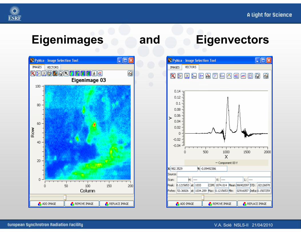
Eigenimages and Eigenvectors

V.A. Solé NSLS-II 21/04/2010
Eigenimages and Eigenvectors

V.A. Solé NSLS-II 21/04/2010
Eigenimages and Eigenvectors
V.A. Solé NSLS-II 21/04/2010
Eigenimages and Eigenvectors

V.A. Solé NSLS-II 21/04/2010
Eigenimages and Eigenvectors
V.A. Solé NSLS-II 21/04/2010
Eigenimages and Eigenvectors

V.A. Solé NSLS-II 21/04/2010
The main PCA application
• Previous example:• Map of 101 rows x 200 columns x 2000 channels
• PCA tells us:• Information can be described with 4 eigenspectra• 101 rows x 200 columns x 4 + 4 x 2000 channels
We can have the relevant information in ~ 500 times less space !!!!!
PCA is a well known technique to reduce data dimensionality

V.A. Solé NSLS-II 21/04/2010
step1
step2
step3
Step 4
Execution plug-in
Control plug-in
Features of EDNA• Pipe-lining tool for on-line data analysis• Enables single-threaded code(e.g existing scientific software) to be used multi-threaded
• Relies on data models• Testing framework
• Unit & Execution tests• Non-regression test before nightly builds
• Plugin-wise programming• Plugin generator• Re-use of plug-ins already written (by others)
• International collaborationAcknowledgements : Olof Svensson

Olof Svensson ISD³ 29/03/2010
EDNA Example: Fast Azimuthal Integration
N x ω 2D Diffraction Images
Fit2D
TADM
SPDXOP
XRDUA
N x ω 1D diffraction patterns
Integration of many tools
Other ?
Acknowledgements : Jérôme Kieffer
Diffraction images (WAXS,SAXS, tomo diffraction etc)
• SPD / Fit2D : 700/800 ms / image• Method from M. Sánchez del Río : 150 ms / image(simple histogramming with numerical noise)
V.A. Solé NSLS-II 21/04/2010
Conclusion
Learn from others’ mistakes, …… life is too short to make them all