Scientific and Technical Advisory Panel · The work was commissioned by the Scientific and Technical Advisory Panel of the Global Environment Facility ... Jean Ann Ramey, ... Keating

Scientific and Technical Advisory Panel

The Scientific and Technical Advisory Panel, administered by UNEP, advises the Global

Environment Facility

March 2013

Calculating Greenhouse Gas Benefits of the Global Environment Facility

Energy Efficiency Projects

Version 1.0.

Acknowledgments

The work was commissioned by the Scientific and Technical Advisory Panel of the Global Environment

Facility (GEF-STAP). The Methodology were prepared by the joint team of the Stockholm Environment

Institute – U.S. (SEI-US) and Synapse Energy Economics, Inc. Step-by-step explanation of GHG calculations

of each module using specific project examples was prepared by Margarita Dyubanova (STAP Secretariat).

Project team:

Michael Lazarus, SEI-US

Chelsea Chandler, SEI-US

Jean Ann Ramey, Synapse Energy Economics

Thomas Vitolo, Synapse Energy Economics

The authors would like to thank Margarita Dyubanova (STAP Secretariat) and David Rodgers (GEF

Secretariat) for their guidance, careful review, and other invaluable input. The authors also greatly appreciate

the helpful feedback provided by STAP members, GEF staff, implementing agency representatives, and

invited experts who attended the GEF-STAP workshop Developing GHG Emission Reduction Methodology for

GEF Energy Efficiency Projects held on February 14-15, 2012, in Washington D. C. that helped to refine the

draft methodology. The following experts provided very helpful early input, including Lev Neretin (STAP

Secretariat), Frank Klinckenberg (Klinckenberg Consultants BV), Richard Hosier, Marcelino Madrigal,

Zhihong Zhang, Marcel Alers (UNDP), Pradeep Monga (UNIDO) and Jas Singh (World Bank), Stephane de la

Rue du Can & Michael McNeil (Laurence Berkeley National Laboratory), My Ton (The Collaborative

Labeling & Appliance Standards Program, CLASP), and Maja Staniec (Wroclaw University of Technology,

Poland).

Table of Contents

I. INTRODUCTION, CONCEPTS AND DEFINITIONS ................................................................ 1

GEF and Energy Efficiency 1

Summary of Key Changes in the Methodology 2

What Distinguishes the GEF Methodology from Other Models for CO2 Accounting? 3

Data Assumptions and Calculation Results 4

Required Data 5

II. STEP-BY-STEP GUIDE TO ESTIMATING THE GHG BENEFITS OF GEF ENERGY EFFICIENCY PROJECTS

7

Step 1: Enter Basic Project Information 7

Step 2: List Activity Components and Select Quantification Model 7

Step 3: Model Activity Components 8

Step 4: Calculate Indirect Top-Down Impacts 12

Step 5. Review the Results 12

ANNEX 1: STEP-BY-STEP EXPLANATION OF GHG CALCULATIONS OF EACH MODULE IN THE METHODOLOGY

USING SPECIFIC PROJECT EXAMPLES ..................................................................................... 14

2.1 Standards and Labeling Module 14

2.2 Building Codes Module 18

2.3 Demonstration and Diffusion Module 22

2.4 Financial Instruments Module 26

ANNEX 2: ADDITIONAL METHODOLOGIES AND RESOURCES FOR QUANTIFICATION OF GHG EMISSION

REDUCTIONS FROM ENERGY EFFICIENCY PROJECTS ............................................................. 29

Calculating GHG Benefits of GEF EE Projects: A Revised Methodology 1

I. Introduction, Concepts and Definitions

GEF and Energy Efficiency

Since 1991, the Global Environment Facility (GEF) has played a major role in supporting energy efficiency

initiatives in developing countries and economies in transition. Through June 2011, GEF provided $1.2 billion in

financing and leveraged $8.5 billion in co-financing to more than 200 energy efficiency projects (GEF COP 17

Report1). The fraction of GEF’s climate change portfolio dedicated to energy efficiency projects has generally

grown over time, comprising 38% in GEF-4 (2006-2010). The World Bank estimated that the GEF energy

efficiency projects implemented by the World Bank, in the period of 1992-2009, have delivered nearly 100 million

tonnes of CO2 equivalent (tCO2e) in direct emission reductions over the lifetime of the projects, and close to 300

million tCO2e in indirect emission reductions2.

GEF requires every climate change project at the ex ante stage (Project Identification Form or PIF) to provide an estimate

of the avoided or reduced amount of greenhouse gas (GHG) emissions the project expected to deliver. In 2008, the

GEF published a Manual describing its methodology for calculating greenhouse gas (GHG) benefits for its energy

efficiency (EE), renewable energy (RE), and clean energy technology projects3. This methodology since then has

provided GEF agencies with a common framework for preparing ex ante (before the event) estimates of potential

GHG benefits verified further during project development and review stages. While representing a strong

foundation, this methodology has nonetheless been open to wide interpretation, providing limited tools and guidance

for consistent calculations, and resulting in a somewhat inconsistent application. At the request of the GEF

Secretariat and its partners, the GEF Scientific and Technical Advisory Panel (STAP) commissioned a study to

review the existing EE methodology, identify its strengths and weaknesses, review alternative approaches, and

develop a revised methodology/algorithm for calculating GHG benefits of GEF EE projects4. The intent of this

proposed revision is to improve the rigor and consistency of the GHG analysis, and to simplify the application of the

methodology for GEF agencies, by providing a more complete, and easy-to-use spreadsheet tool that embeds more

standardized guidance in the form of algorithms and conservative default factors.

Section 1 and 2 discuss the impetus and process for revising the methodology for EE projects, and summarizes key

changes to the existing methodology. Section 3 provides step-by-step instructions for applying the updated

methodology to calculate potential GHG emission savings associated with GEF energy efficiency projects. Annex 1

provides examples for calculating GHG benefits in each module of the methodology, while Annex 2 lists other

existing tools and methodologies relevant to estimating GHG emission benefits of energy efficiency projects.

STAP and GEF identified the following criteria to guide the revision of the existing RE and EE methodology:

Simplicity, and minimizing the level of effort required to apply the methodology;

Availability and ease of data collection;

Applicability to a broad range of energy efficiency projects;

Consistency among projects;

Significance, in order to ensure a greater focus on material impacts;

1 Available at: http://unfccc.int/resource/docs/2012/cop18/eng/06.pdf

2 Hosier, R. (2010). Laying the Foundation for a Low Carbon Future: The World Bank-GEF Partnership.

3 GEF (2008). Manual for Calculating Green House Gas Benefits of GEF Project: Energy Efficiency and Renewable Energy

Projects. Available at http://www.thegef.org/gef/sites/thegef.org/files/documents/C.33.Inf_.18%20Climate%20Manual.pdf 4 The initial RE and EE methodology (footnote 3) remains relevant for calculating GHG benefits of the GEF renewable

energy projects.

http://unfccc.int/resource/docs/2012/cop18/eng/06.pdf

http://www.thegef.org/gef/sites/thegef.org/files/documents/C.33.Inf_.18%20Climate%20Manual.pdf


Credibility, as reflected in reliance on accepted methods or credible literature and data sources.

Summary of Key Changes in the Methodology

The major changes to the GEF’s methodology for EE projects resulting from the application of the above criteria,

review of relevant methodologies, and other research are as follows:

“Modules” were introduced into a new methodology to allow for component-specific calculations of

emission reductions. In the revised methodology, activity proponents have four modules to choose from:

1) Standards and Labeling, 2) Building Codes, 3) Demonstrations and Diffusion, and 4) Financial

Instruments - with simple algorithms reflecting the unique attributes of each intervention type. The

spreadsheet is designed so that the proponents distinguish activity components and outputs that could have

a discernible GHG emission benefits, and then select specific module/s that represent them best. In

developing this methodology, over 20 GEF project documents were reviewed by the project team leading

to the conclusion that nearly all of the typical GEF EE activity components could be assigned to one or a

combination of the proposed four modules. In many instances, projects involve multiple components–

combining for example, demonstration projects, with development and enhanced enforcement of a building

code. The spreadsheet is designed to enable project proponents to combine multiple activity components

(up to 10 within each module), with reporting of results for individual components as well as cumulatively

for the entire project. The attributes for each of these modules are discussed in the following section.

Added capabilities and specification of direct, direct post-project, and indirect GHG emission savings

were introduced. For example, the revised methodology enables the calculation of the direct, post-project

emission reductions associated with policies such as standards and codes, where the policy is established

prior to project closure and for GHG savings resulting from equipment purchases or new construction after

project closure.

The new methodology includes default factors and encourages project proponents to use project-

specific dynamic baselines. In practice, some project documents have done a thorough and conservative

job of accounting for autonomous improvements in energy efficiency independent from GEF intervention,

while others have not explicitly considered such “independent” from the GEF changes in the project

baseline. The revised methodology provides simple, standard algorithms that require the User to specify

levels of energy efficiency improvement, penetration of energy efficient equipment, levels of building code

compliance, and/or the fraction of activity undertaken likely to occur in a business-as-usual scenario

without GEF intervention. In addition, it provides default values, such as an assumed 1% improvement per

year in baseline efficiency, which can be revised by users with an appropriate justification.

Additional default values are introduced to simplify calculations. Examples include 1) a selectable

database of grid electricity emission factors (based on the CDM combined margin methodology)5, 2) an

avoided transmission and distribution loss factors for electricity saving projects (often not included in the

5 The revised methodology suggests default use of the combined margin grid electricity factor, as established in CDM

methodologies, as a default for EE projects. Marginal emission factors, that reflect the types of electricity generation that is more likely to be displaced by (operated less and/or not built) are more appropriate for estimating emission reduction

impacts than the average emission factors commonly presented in national statistics (World Resources Institute and World Business Council for Sustainable Development (2007). Guidelines for Quantifying GHG Reductions from Grid-Connected Electricity Projects. Washington, DC.). More sophisticated approaches than the CDM grid emission factor methodology are

possible, taking into account the load shapes of the energy efficiency activities, and using information on hourly or seasonal variation in emissions of marginal units (e.g. via dispatch analysis) and can provide more accurate estimates (e.g., Vine, E., Hall N., Keating K., Kushler M. , and Prahl R. (2012). Emerging Issues in the Evaluation of Energy-efficiency Programs: The

US Experience. Energy Efficiency 5: 5–17).


current project descriptions), and 3) fossil fuel combustion emission factors (based on the IPCC Good

Practice Guidance6).

In addition, the Standards and Labeling module contains illustrative default values for dozens of efficient

technologies, such as CFL and LED lighting, numerous appliances, and industrial motors and boilers, along with

values for the corresponding standard technologies that they would displace. Default values are available for power

consumption, usage hours per day, and days of use per year and represent estimates for a single developing region at

a particular point in time. They provide illustrative starting values that could be replaced, as appropriate, with

current values developed for the specific project in question.

What Distinguishes the GEF Methodology from Other Models for CO2 Accounting?

One of the basic features of the GEF’s GHG emission reduction quantification methodology has been the distinction

between direct and indirect emission reductions. Direct GHG emission reductions are those achieved by project

investments such as technology demonstrations and discrete investments financed or leveraged during the project’s

supervised implementation period (from the project start to the project closure). In contrast, GHG emission

reductions achieved, for example, as a result of market facilitation and development through project-supported

policy and institutional frameworks, capacity building, information gathering, and replication effects of

demonstration activities, are considered indirect GHG emission reductions. In addition, a third category, direct

post-project emission reductions, has been used to quantify the GHG emission reductions of GEF-supported

revolving financial mechanisms that are still active after the project’s closure (ex post).

These categories have different accuracy of GHG emission reduction estimates, with the direct emission reductions

presumed to be the most accurate and certain, followed by direct post-project emission reductions, and finally,

indirect. However, in GEF practice GHG accounting for these emission categories was not applied systematically

confusing the cumulative impact of GEF investments with respect to GHG emission reductions. The ad-hoc review

of some GEF EE projects revealed that several market facilitation and policy-based projects—mostly, for efficiency

standards and labeling projects—have reported the resulting emission reductions as direct, rather than indirect, as

the manual would suggest should be done. If, indeed, standards were to be adopted, with enforcement systems, it

would be hard to argue that the estimated emission reductions are less certain and attributable to GEF than many

other project outputs that are currently considered to lead to direct impacts, such as financing to support ESCO

projects. The review also found that direct post-project emissions benefits have been reported for non-financial

projects, such as dissemination of results from demonstration projects, more often than for the revolving fund

projects for which this accounting category is intended to apply.7

In order to address the above inconsistency, the revised methodology takes a different approach to the estimation of

direct and indirect GHG emission reductions. First, the revised methodology introduces four modules enabling

analysis of the GHG emission reductions for the key existing types of GEF support for EE projects: standards and

labeling, building codes, demonstration and diffusion, and financial instruments. In all the modules, policy

implementation activities are now explicitly capable of generating direct emissions benefits. For projects where

building codes, standards, and labeling components lead to building EE improvements and equipment purchases

prior to the project closure, the resulting emission reductions (over the lifetime of those improvements and

purchases) are considered as direct project impacts. Building improvements and equipment purchases that occur

6 IPCC. (2006). “2006 IPCC Guidelines for National Greenhouse Gas Inventories.” http://www.ipcc-

nggip.iges.or.jp/public/2006gl/index.html. 7 See for example, commercial buildings project in Thailand (GEF ID 4165) and residential and commercial buildings project

in Namibia (GEF ID 3793).

http://www.ipcc-nggip.iges.or.jp/public/2006gl/index.html

http://www.ipcc-nggip.iges.or.jp/public/2006gl/index.html


after project closure are considered to result in direct post-project impacts. As a result, in the revised methodology,

policy implementation projects are treated similarly to projects involving specific investments.8

The earlier methodology provided two options for calculating indirect GHG reduction benefits. The bottom-up

method involves multiplying direct emission reductions by a replication factor (RF), intended to reflect how many

times the investments achieved during the project period might be repeated during an “influence period” (e.g., 10

years) after the project closure. The top-down method involves multiplying total market potential for CO2 emission

reductions by a causality factor (CF). Market potential combines technical and economic market potential for the

technology within the 10 years after the project’s lifetime. CF is the percentage of a realized market potential that

can be reasonably attributed to the long-term effect of the project as the result of overcoming market barriers.9

The revised methodology allows estimating both top-down and bottom-up indirect GHG benefits. The top-down

estimate is based on a single market potential analysis and is performed at the project level (as opposed to the

module level). In contrast, the bottom-up indirect estimate is calculated for individual activity components. For

projects involving demonstration and diffusion activities, or the use of investment instruments, the User can specify

(by providing justification) the number of expected replications during the post-project influence period, on a

component-by-component basis for each component (e.g., an ESCO or a green building demonstration project).

Data Assumptions and Calculation Results

The project proponent should err on the side of transparency, and generally be cautious and conservative when

making assumptions about GHG emission reductions. The calculation produces both, annual and cumulative results.

The spreadsheet presents the results separately for project and post-project periods, including for specific years that

users can select.

Currently, CO2 is the only GHG considered in this methodology. For energy efficiency projects, in most cases,

where avoided fossil fuel combustion is the principal source of GHG emission reductions within the project

boundaries, trace emissions of methane and nitrous oxide from incomplete combustion are quite small (less than 1-

2% or less of overall CO2-equivalent emissions or emission reductions). Where there is a significant on-site leakage

of natural gas or biological methane, such emissions could be significant and should be considered in the estimate.

This is the case, for example, with the climate benefits of projects that reduce GHG emissions through improved

charcoal production (methane and nitrous oxide reductions) or support technologies and frameworks reducing

emissions of ozone depleting substances (HFC and HCFC reductions). Where non-CO2 GHGs are considered, the

100-year global warming potentials from the Intergovernmental Panel on Climate Change (IPCC) Fourth

Assessment Report10

should be utilized. While the revised methodology does not provide any calculation tools for

these emissions benefits, the “Results” tab in spreadsheet provides a place to enter them.

8 The treatment of standards, labeling, and codes in the category of indirect emission reduction in the earlier methodology

may had impacted the certainty and accuracy of emission reduction estimates because indirect methods used in these calculations generally involve the use of rather speculative replication factors (bottom-up approach) and/or the estimated market potential data (top-down approach). Well-vetted methods for quantifying the benefits of these policies already exist

and have started to be applied by GEF making it possible in the revised methodology to count these emission reductions as direct emission reductions. 9 The earlier methodology implied that conducting both top-down and bottom-up analyses can provide a range of estimates

that would represent the uncertainties in indirect emissions estimation; however, only some projects in the studied cohort reported a range. While informative and theoretically appealing, the range itself does not serve as a good indication of the underlying uncertainties in indirect emission calculations. Furthermore, the bottom-up result in many cases nearly matches

or exceeds the top-down result, suggesting that this exercise does not tend to “bound” the indirect estimate, and may lead to questionable results. 10

IPCC 4th Assessment Report is available at http://www.ipcc.ch/publications_and_data/ar4/wg1/en/ch2s2-10-2.html.

http://www.ipcc.ch/publications_and_data/ar4/wg1/en/ch2s2-10-2.html


More holistic GHG accounting approaches consider life-cycle emission impacts. A possible step in this direction

would be to include full life-cycle emission factors for fuels, accounting for emissions from well or extraction point

to the point of combustion. Such values can be entered directly into the spreadsheet. A more complete analysis

would consider life-cycle emissions for the equipment and construction involved in the project. Both of these

approaches, while potentially informative, would substantially increase the level of effort required, introduce

significant uncertainties, and go beyond commonly used approaches of project-specific GHG accounting.

Required Data

The following data requirements and assumptions are common to all the modules in the methodology.

Baseline scenarios: Robust assessment of GHG benefits of the GEF EE project depends on the determination of a

dynamic baseline scenario, representing the likely evolution of energy-efficient technologies and practices without

GEF intervention. The baseline scenario should be carefully presented in the project document. The revised

methodology focuses on specific calculation techniques that can be used to ensure consideration of the likelihood

that some improvements will occur in the absence of GEF intervention (see Error! Reference source not

found.)11, for example:

o 1% improvement per year in relative efficiency of baseline technology (e.g., unit energy intensity

of the baseline technology would decline by 1% per year)

o increase in market share of improved efficiency (project) equipment of 5% per year.

Emission factors: The spreadsheet provides default fuel-specific emission factors drawn from the IPCC 4th

Assessment Report12

. It also contains a database of country-specific electricity emission factors developed under the

CDM13

. Users can overwrite these defaults if more specific information is available.

Lifetimes of investments and technologies: The investment-specific parameter that needs to be determined is the

lifetime of the investment or technology deployed. For various operational programs, different technologies,

investment conditions, and assumptions are appropriate. The methodology carries over the default from the earlier

methodology, highly-generic five year lifetime for appliances. For other technologies, the User should enter and

document an appropriate, conservative assumption for the investment lifetime.

11 As noted by many observers, there can be a tendency by GEF project proponents to understate the likely improvements

that might occur under business-as-usual conditions, for example, without the proposed GEF intervention leading to inflated estimation of GEF-specific contribution to GHG emission reductions. 12

IPCC. (2006). “2006 IPCC Guidelines for National Greenhouse Gas Inventories.” http://www.ipcc-nggip.iges.or.jp/public/2006gl/index.html. 13

See discussion document for the rationale for using these defaults (Lazarus et al. (2012). Revising GEF’s GHG Methodology for Energy Efficiency Projects. A Discussion Document for the GEF STAP Workshop (February 14, 2012, Washington DC), Feb. 8 Draft. Stockholm Environment Institute – U.S. & Synapse Energy Economics, Inc.).

.


Table 1. Overview of the Methodology Modules

Standards and Labeling Building Codes Demonstration & Diffusion Financial Instrument

General applicability

conditions

Projects that systematically address

energy using equipment or devices

through standards, labeling or other

changes to regulatory and industry

structures

Projects that systematically address

residential, public, or commercial

sector building efficiency through codes or other policy instruments

Projects that include demonstration to

strengthen awareness, knowledge, and

capacity building; or diffusion that helps

to bring about broader use of an energy-

efficient technology

Projects that involves direct finance of

EE investments or support to financial

intermediaries; interventions cannot be

easily reduced to common

technologies and penetration rates, given diversity of industries, etc.

Intervention types

Standards and labeling; minimum

efficiency performance standards

Building code establishment; enhanced

code enforcement

Technology demonstration and capacity

building; technology development and diffusion

Financing mechanisms (loan or

revolving funds); ESCO creation/support

Project examples

Appliances (e.g., refrigerators,

washing machines, air conditioners.

etc.); lighting; space heating and

cooling

Insulation, enhanced construction, cool roofs

New building with energy efficiency

technologies; retrofit of a building or a

set of buildings; implementation of

energy management plans and system optimization activities in enterprises

Promoting energy efficiency markets

in industrial, commercial, and public buildings sectors

Typical data

requirements

Targeted and displaced technologies;

either technology power and activity

or unit energy consumption; year

standard enters into force; percent of new sales compliant with standard

Target and displaced technologies;

either technology power and activity or

energy consumption per area

(kWh/m2); the year building code

enters into force; percent of affected

buildings compliant with the code

MWh or GJ savings per “unit” (e.g., per

building, foundry, optimization

completed, etc.); activity levels (number of “units” replicated each year

MWh or GJ savings per investment

unit (e.g., US$); investment in each year

Typical project-specific

data sources

Surveys and audits; national statistics;

available scenario analyses; manufacturer data

Surveys and audits; national statistics;

available scenario analyses; manufacturer data

Energy audits; surveys; national

statistics

Audits; market studies of investment

effectiveness, ESCO returns, etc.

Algorithms

Stock model based on technology

sales and penetration rates

Model based on affected building area

(m2) and penetration rates

Savings per unit multiplied by number

of units deployed

Simple ROI model: savings per unit

investment multiplied by amount invested

Baseline approach (with

default values, where

provided in parenthesis)

Annual sales and growth rate for

technology/equipment

Annual improvement in relative

efficiency of baseline technology

(1%/year)

Annual increase in improved

technology penetration (5%)

Annual affected building area (m2) and

growth rate

Improvement in relative efficiency of baseline technology (1%/year)

Percent compliance with building code

(where it currently exists)

Existing building energy intensities

Percent of activities implemented in the baseline (i.e., that would have occurred

anyway in absence of the project) (10%)

Other defaults available

Illustrative defaults for about 30

technologies (power consumption and

usage characteristics)


II. Step-by-Step Guide to Estimating the GHG benefits of GEF Energy Efficiency Projects

This section provides step-by-step instructions for using the Excel spreadsheet tool to calculate avoided GHG emissions from GEF

energy efficiency projects.

The Basic Guide tab of the spreadsheet contains a description of the tabs and the types of information contained in each tab:

Yellow tabs are working tabs where the User inputs data;

Blue tab is the results tab where the User can see the overall results of calculation;

Black tabs are reference tabs for User’s information.

The Basic Guide also illustrates various functions of cells based on the color:

User-input cells

User-input cells with a pull-down menu

User-input cells that differ from default values

Cells not intended for User input

Cells not appropriate for input or output

Step 1: Enter Basic Project Information

Complete the Project Info tab in the spreadsheet tool by entering basic project information data. In addition, the User needs to

specify the following general parameters:

1) Length of the analysis period in year after the project closure – not to exceed 20 years.

2) Maximum technology/Measure lifetime – the default maximum is set at 20 years.

3) Fuel type(s) and emission factors14

– the User can choose up to three fuels in addition to electricity by accessing the pull-

down menu. Once the fuel is chosen, its associated emission factor15

will automatically fill in the both the “Default” and

“User Specified” fields. As with all defaults, the User can overwrite the value in the User Specified cell. If a project uses a

fuel not listed, the User can add the fuel and emission factor by editing values in the black tab entitled “Fuels”. Rather

than adding a row to the table, the User should replace data in the table for one of the fuels not used in the project.

Step 2: List Activity Components and Select Quantification Model

In Project Info tab, the User should list the Activity Components and select a corresponding quantification module.

1) List Activity Components – the User should list activity components for which emission reductions are being

quantified. Please note that not all Activity Components have to match the Project Components in the Project

Logframe table in the PIF. Activity Components help break down GEF Project Components into separate

14

Default values in the model were chosen to be conservative and consistent. The use of alternative values should be justified and documented with the explanation in the “Notes” section of the spreadsheet tool itself.

15

Derived from the 2006 IPCC Guidelines for National Greenhouse Gas Inventories.


quantification steps when the characteristics of the activities within a component vary. The Activity Components

titles will appear in the table headings throughout the model.

Enter Sector/Subsector and Logframe Output, then Select Module/Intervention Type–from pull-down menu the User should select

the module that best fits each Activity component There are four different modules available for estimating GHG emission

reductions associated with the GEF energy efficiency projects:

1) Standards and Labeling,

2) Building Codes,

3) Demonstration and Diffusion, and

4) Financial Instruments.

The User begins by listing all key activity components that could yield emission reductions followed by the module selection that

is most appropriate for each component.

The Standards and Labeling and Building Codes modules are both appropriate for market transformation projects that

implement changes to existing regulatory and industry structures. Building codes characterize goals in kilowatt-hours saved per

square meter (kWh/m2), while standards and labeling projects will express savings per unit (e.g., refrigerators, motors) and ask for

the number of units to be installed under the project.

The Demonstration and Diffusion module is appropriate for: 1) projects that are intended to be used as a technology

demonstration to strengthen awareness, knowledge, and capacity building, such as a new building with multiple energy efficiency

technologies, or a retrofit of a building or a set of buildings; and 2) diffusion projects that help to bring about broader use of an

energy-efficient technology, such as projects that make a specific energy-efficient technology available at a cheaper price. This

module is quite flexible and can be applied for many different types of activity components where savings are estimated based on

an expected number of activities or investments.

The Financial Instruments module is appropriate for projects that involve investments and financing mechanisms when energy

savings may result from discrete activities where the technologies, sectors, or end use may be difficult to predict (e.g., ESCOs or

loan instruments), or from replication of pilot and demonstration activities.

Step 3: Model Activity Components

Standards and Labeling Module

In the Standards and Labeling tab the User will find tables for each Activity Component listed under “Standards and Labeling”

module in the “Project Info” tab. For each Activity Component, the User should enter several key variables, including:

1) Target technology–from drop-down menu the User should choose the fuel used by target technology and displaced

technology. The User may overwrite the default in the User-Specified column by selecting a fuel from the drop-down

menu. Only those fuels selected in the Project Info tab will appear as fuel choices here.

2) Displaced technology–the User may overwrite the default displaced technology but must enter the corresponding Power

Consumption (in watts for electricity, MJ/hour for other fuels) of the displaced technology in the “Calculate Annual

Energy Consumption” table

3) Useful technology lifetime in years (less than or equal to the Maximum Lifetime entered in the Project Info tab)

As an example, consider a project on standards and labeling in which LEDs will replace incandescent lighting. While the default

“Displaced Technology” associated with a LEDs projects is CFLs, the User can type in any alternative, (in this example,

incandescent bulbs). The title “incandescent” will flow through to the Power Consumption row and the value should be updated by

the User.

The model contains illustrative default values for more than two dozen efficient technologies, numerous appliances, and industrial

motors and boilers, along with values for the corresponding standard technologies that they would displace. Default values are


available for: usage hours per year, average power consumption. These values represent estimates for a single developing region at

a particular point in time. They provide illustrative starting values that should be replaced, as appropriate, with current values

developed for the specific project in question.

For annual energy consumption, the User should choose between:

(Option 1) allowing the model to calculate annual energy consumption, OR

(Option 2) entering the annual energy consumption for the target technology and the displaced technology.

When using Option 1 (model-calculated energy consumption), the User should enter power consumption for each technology, in

addition to technology usage data. Those values flow through to the following rows, which calculate annual energy consumption.

For Option 2, if the annual energy consumption of the target technology and the displaced technology are known, the User should

enter them directly in the final rows under “Technology Specifications” table.

The model is designed to represent a dynamic baseline, indicating natural adoption of the target technology that would have been

happening in the absence of GEF intervention, and the rate of performance improvement for both, the target and the displaced

technology. The tables entitled Market Assumptions, Baseline Assumptions, and Standard/Labeling Project Effectiveness,

contain proxy values to be used in these calculations. Ideally, the User would provide the following inputs:

1) Annual sales in first year (expected sales of all units, both the target and displaced technology);

2) Annual sales growth rate (percentage);

3) Market share of target technology in first year;

4) Baseline annual increase in target technology market share;

5) Annual reduction in energy consumption for the target technology;

6) Annual reduction in energy consumption for the displaced technology;

In addition, the model accounts for standards project effectiveness with the following inputs:

1) Year the standard is put in place;

2) Percent compliance with new standard

In the table entitled “Annual Inputs and Calculations” (for which the User should scroll to the right), the top row shows the total

units of the technology (both target and displaced) sold annually. These figures are based on market assumptions. The total annual

sales of the target technology for each year of the project can be entered manually if the actual market share of the target

technology is expected to deviate from the values calculated by the model (e.g. if sales in early years are expected to be slower

than the average of sales across all project years). The User would input values directly in the row entitled “MARKET Annual

Sales (Units)”. Once the value in the initial cell has been altered, the subsequent values will auto-update based on the percentage

growth rate in Market Assumptions. The User should overwrite all cells in the row to ensure accurate accounting.

Also in the “Annual Inputs and Calculations” table the User can view the tabulation of the project emissions, baseline emissions,

and the difference between the two (delta or savings) for each year, along with the cumulative avoided greenhouse gas emissions.

For standards and labeling activities, the module distinguishes direct and direct post-project impacts, based on the timing of

equipment purchase. Energy and emission savings associated with equipment or appliances purchased prior to the date of project

close are considered direct project impacts, while those savings associated with purchases after this date are considered direct post-

project impacts.

There is no indirect bottom-up calculation for this module. Indirect, spillover benefits from the establishment of standards and

labeling, e.g. in the form of more stringent standards or extension to additional products after project close, are best represented

through a market potential assessment, and thus are addressed through the top-down indirect calculation (see Step 4 below).


Cumulative and annual project results for all components are summarized in the table titled “Results: Standards and labeling

Activity Components” directly below the ”Project Information” table in the “Standards and Labeling” tab.

Building Codes Module

In the Building Codes tab the User will find tables for each Activity Component listed under “Building Codes” module in the

“Project Info” tab. For each Activity Component, the User should enter several key variables, including:

Target technology;

1) Fuel used;

2) Displaced technology;

3) Useful technology lifetime (years)16

The User should choose between:

(Option 1) allowing the model to calculate annual energy consumption, OR

(Option 2) entering the annual energy consumption for the target technology and the displaced technology.

If using Option 1 (model-calculated energy consumption), the User should enter power consumption per square meter of building

space for each technology.

The model is designed to represent a dynamic baseline, indicating natural adoption of the target technology that would have been

adopted in the absence of GEF intervention and the rate of performance improvement for both the target and the displaced

technology. To do this, the following inputs are required:

1) Annual floor area affected in first year;

2) Annual affected floor area growth rate;

3) Market share of target technology in first year;

4) Baseline annual increase in target technology market share;

5) Annual reduction in energy consumption for the target technology;

6) Annual reduction in energy consumption for the displaced technology;

In addition, the model accounts for effectiveness of the building code project with the following inputs:

1) Year the building code is put in place;

2) Percent compliance with new code

Finally, the area of building floor space to be affected in each year of the project can be entered manually if the actual market

share of the target technology is expected to deviate from the values calculated by the model (e.g. if affected area in early years is

expected to be slower than the average of affected area across all project years). To enter this data, the User should scroll to the

right to the annual data table for each component. To do this, the User should input values directly in the row entitled “Market

Annual Sales (Units)”. Once the value in the initial cell has been altered, the subsequent values will auto-update based on the

percentage growth rate in market assumptions. The User should overwrite all cells in the row to ensure accurate accounting.

Also in the “Annual data” table, the User can view the tabulation of the project savings, baseline savings, and the difference

between the two (delta) for each year, along with the cumulative avoided greenhouse gas emissions. The building code activities

16

While some applications such as insulation, thermal breaks and other construction techniques may have lifetimes longer than 20 years, it is important to consider the forecasting difficulties and uncertainty inherent in the results, making it inappropriate to attempt to capture savings from those longer timelines; as is the case with the deviation from any default values, robust documentation should accompany the

new values in the notes section of the model.


module distinguishes between direct and direct post-project impacts, based on the timing of equipment purchase. Energy and

emission savings associated with buildings built or retrofit prior to the date of project close are considered direct project impacts,

while those savings associated with purchases after the project close date are considered direct post-project impacts.

There is no indirect bottom-up calculation for this module. Indirect, spillover benefits from the establishment and enforcement for

building codes (e.g., in the form of more stringent codes or more effective enforcement) are best represented through a market

potential assessment, and thus are addressed through the top-down indirect calculation (see Step 4 below).

Cumulative and annual project results for all components are summarized in the table titled “Results: Building Codes Activity

Components” directly below the ”Project Information” table in the “Standards and Labeling”

Demonstration and Diffusion Module

In the Demonstration and Diffusion tab the User will find tables for each Activity Component listed under “Demonstration and

Diffusion” module in the “Project Info” tab. For each Activity Component, the User should enter several key variables, including:

1) Energy savings per user-specified unit for each fuel (e.g., per building, foundry, optimization completed, etc). The User

may note in the Notes section the unit for which the savings are calculated.

2) Lifetime of investment (years);

3) Baseline assumption (% of activities implemented absent GEF intervention);

4) Number of replications post-project as spillover (necessary for the indirect bottom-up estimate);

5) Number of units to be installed in each year of the project.

To enter the last input, the User should scroll to the right in the spreadsheet. For each component listed in the “Project

Info” tab, there is an “Annual Inputs and Calculations” table. The top row of that table (labeled “Project”) requires annual

input from the User. For each year of the project implementation period, input the number of units that will be installed in

each year of the project. This step should be repeated for each component of the project.

For each year, total savings are calculated by the spreadsheet by multiplying the total units that have been installed to date (and are

still within their useful lives) by the savings per unit.

In the “Annual Inputs and Calculations” table the User can also view the cumulative direct savings by fuel, the total cumulative

direct savings, and the indirect bottom-up savings.

Cumulative project results (including all components) are also summarized in the table directly below the “Project Information” in

the “Demonstration and Diffusion” tab.

Financial Instruments Module

In the Financial Instrument tab the User will find tables for each Activity Component listed under “Financial Instrument” module

in the “Project Info” tab. For each Activity Component, the User should enter several key variables, including:

1) Monetary unit;

2) Energy savings for each fuel per user-specified monetary unit;

3) Lifetime of investment in years;

4) Baseline assumptions, including percent of activities implemented absent GEF intervention;

5) Number of replications post-project as spillover;

6) Amount of money to be invested in each year of the project.

To enter the final input, the User should scroll to the right to view the annual data table for each component.

For each year the total savings are calculated by multiplying the total monetary amount that has been invested to date by the

emission savings per investment.


In the “Annual Data” table, the User can view the tabulation of the project savings, baseline savings, and the difference between

the two (delta) for each year, along with the cumulative avoided energy use and greenhouse gas emissions during the project and

post-project periods.

Cumulative project results (for all activity components) are also summarized in the table directly below the “Project Information”

table in the “Financial Instrument” tab.

For some projects, one project instrument could have different expected investment returns. The current model addresses this issue

by allowing multiple components (to be input in the “Project Info” tab) within each module. For example, in the financial module,

an ESCO that address commercial building efficiency and industrial efficiency could expect a return of 7 MWh per $1,000

invested on the commercial building components and 5 MWh per $1,000 invested on the industrial components. The User might

list one component as “ESCO commercial” and the other as “ESCO industrial” in “Project Info” tab.

Step 4: Calculate Indirect Top-Down Impacts

The indirect top-down estimates can be developed in the table on the top of the “Results” tab. Since multiple activity components

may target similar technologies, practices, sectors and end-uses, indirect top-down estimates are assessed at the project level,

rather than by each Activity Component. To estimate indirect top-down estimates, the User should enter the following two

variables:

1) Total market potential (tCO2).

Enter total market potential for CO2 emission reductions, based on market studies or scenario analysis, achievable during

the 10 year project influence period after project closure.

2) Causality factor (CF).

Indicate the level of attribution of the GEF intervention to full market

The User should carefully consider and document the expected causality of the GEF project in achieving the full market potential.

The User should take intoaccount that some or all market potential may be achieved without a GEF intervention due market forces

or government policies beyond those created by the project. For the GEF Causality Factor, five levels of GEF impact and

causality are suggested:

Level 5 = 100 % The GEF contribution is critical and nothing would have happened in the baseline.

Level 4 = 80 % The GEF contribution is dominant, but some of this reduction can be attributed to the baseline.

Level 3 = 60 % The GEF contribution is substantial, but modest indirect emission reductions can be attributed to the

baseline.

Level 2 = 40 % The GEF contribution is modest, and substantial indirect emission reductions can be attributed to the

baseline.

Level 1 = 20 % The GEF contribution is weak, and most indirect emission reductions can be attributed to the baseline.

While the GEF Causality Factor is useful and can deliver consistent results, GEF Causality Factors should rely on situation-

specific justifications and be estimated conservatively, and deviate from the percent values shown above. Users should provide a

narrative with reasoning and justification of their choices in the “Notes” section.

Step 5. Review the Results

Once Steps 1-4 have been completed, the User can review and report the total results shown in the “Results” tab. Proponents are

suggested to refer to other project documents and reports on energy efficiency, to ensure that results are of the correct order of


magnitude according to the scale of project. Given large uncertainties inherent in ex ante estimation, the User should also bear in

mind that results are shown with more significant digits than warranted.. Therefore, figures should be rounded to no more than 2

significant digits when reporting the results.


Annex 1: Step-by-step explanation of GHG calculations of each module in the methodology

using specific project examples

2.1 Standards and Labeling Module

PROJECT TITLE: LIGHTING MARKET TRANSFORMATION

COUNTRY: Peru

GEF GRANT: $1,636,000

CO-FINANCING: $8,864,000

DATES OF IMPLEMENTATION: 2011-2015

The aim of the project is to enhance promotion and implementation of utilization of energy saving lamps (ESLs) through the

transformation of the local lighting products market and the phasing-out of incandescent lamp (ILs) imports and sales.

The project consists of two components:

Component 1: Market Development

The barriers concerning the marketing and promotion of ESLs and the phasing out of IL production and sales are planned to be

addressed in this project component. Several activities include: (i) substitution of ILs for Compact Fluorescent Light (CFL)s,

comprising about 5 million CFLs, (ii) public lighting schemes to promote energy efficiency lighting technologies (substitution of

mercury lamps for sodium lamps) and rationalization of lighting schemes, comprising the distribution and installation of about 1

million ESLs.

Component 2: Policy and Institutional Support Program

This component will support transformation of lighting market with a coherent ESL policy in line with Peruvian governmental

policies.

Table 1 presents an extended data that were collected during the project concept preparation:

Unit Value

Maximum Technology / Measure Lifetime years 5

Target Technology CFL

Displaced Technology IL

Power Consumption of CFL W 15

Power Consumption of IL W 60

Daily Usage Hr/day 5

Days Used Each Year day 350

Annual Energy Consumption (CFL) kW/year 26

Annual Energy Consumption (IL) kW/year 105

Annual Sales in Year 2011 units 42,612,000

Annual Sales Growth Rate % 2.7

Market Share of CFL in Year 2011 % 20.2

Baseline Annual Increase in Market Share of CFL % 1.66

Annual Reduction in Energy Consumption (CFL) % 0


Annual Reduction in Energy Consumption (IL) % 1

Year Standard in Force year 2015

Percent New Sales Compliant with the Standard % 100

Step 1. Enter Project Information in “Project Info” tab.

The Guide provides explanation for the cell colors:

User-input cells





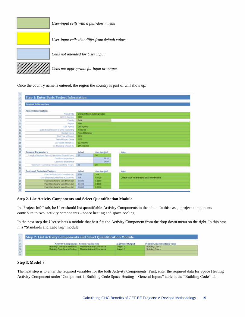
Once the country name is entered, the region the country is part of will show up.

Step 2. List Activity Components and Select Quantification Module

In “Project Info” tab, he User should list quantifiable Activity Components in the table. Both project components contribute to one

activity component.


In the next step the User selects a module that best fits the Activity Component from the drop down menu on the right. In this case,

it is “Standards and Labeling” module.

Step 3. Model Activity Components

The next step is to enter the required variables for the Activity Component.

Step 4. Calculate Indirect Top-Down Impacts

Enter Total Market Potential in tonnes of CO2 and the Causality Factor of the project in the “Results” tab.

Step 5. Review Overall Results

The results table in the “Results” tab shows overall results for all modules (or all activity components). In case of this project, the

results table shows the results of quantification the Standards and Labeling module as it is the module that was used to quantify the

impacts of the project components.


The results of the GHG emissions reduction show:

Direct emission reductions achieved during the project length;

Direct Post-Project emission reductions achieved during project influence period of 20 years after the project close date;

Indirect Top-Down reductions achieved through the causal influence of project at the national level.


2.2 Building Codes Module

PROJECT TITLE: ENERGY EFFICIENT BUILDING CODES

COUNTRY: Syria

GEF GRANT: $3,450,000


DATES OF IMPLEMENTATION: 2010 - 2014

PROJECT DESCRIPTION

The project objective is to reduce GHG emissions through implementation of energy efficient building codes for new construction

in Syria. The project has a goal to establish new Building Code that is expected to set minimum standards for buildings’ heating

and cooling demand only, thereby primarily affecting the energy consumption of space heating, air-conditioning and ventilation.


Unit Value

New Construction in 2010-2015 mill. m2 107

Average Construction Growth Rate % 15

Grid Electricity Emission Factor17

t CO2/MWh 0.712

Share of new building area in compliance with BC % 5

New area in compliance with BC mill. m2 5.355

Average baseline heat demand for space heating (covering

80% of the total area) kWh/m2 127

Annual Reduction in Baseline Energy Consumption for

Heating % 4

Assumed new building code (BC) requirement for space

heating kWh/m2 51

Average baseline electricity consumption for AC&V (covering

60% of total area) kWh/m2 17

Annual Reduction in Baseline Energy Consumption for

Cooling % 1

Assumed new BC requirement for cooling kWh/m2 11

Step 1. Enter Project Information in “Project Info” tab


User-input cells

17

For the grid emission factor, a gradual reduction from 0.824 kgCO2eq/kWh in 2007 (calculated on the basis of the reported fuel

consumption of the Syrian power plants and the net electricity consumption in 2007 as per the latest IEA annual statistics and the 2006 IPCC emission factors for different fuels) to around 0.60 kgCO2eq/kWh in 2030 is expected from a gradual improvement of the power generation and distribution efficiency and the share of different fuels in power generation. The model allows to enter to enter a static

emission factor in the “Project Info” tab. Thus, we will enter the average of two emission factors, 0.712 kgCO2eq/kWh.








In “Project Info” tab, he User should list quantifiable Activity Components in the table. In this case, project components

contribute to two activity components – space heating and space cooling.


it is “Standards and Labeling” module.

Step 3. Model s

The next step is to enter the required variables for the both Activity Components. First, enter the required data for Space Heating

Activity Component under ‘Component 1: Building Code Space Heating – General Inputs” table in the “Building Code” tab.


Then enter the required data for Space cooling Activity Component under “Component 2: Building Code Space Cooling – General

Inputs” table in the “Building Code” tab.


In the “Results” tab of the spreadsheet, enter total market potential for CO2 and the Causality factor.


The results table in the “Results” tab shows the overall results for all modules. In case of this project, the results table shows the

results of the two components listed under “Building Codes”.


Direct emission reductions are achieved from the adoption of the requirement for new Building Code for construction

activities starting the year when the code is in force.

Direct Post-Project emission reductions are direct reduction achieved after project close date.

Indirect Top-Down emission reductions are achieved from the building code enforcement for the period after the project

close date.

There are no Indirect Bottom-Up emission reductions from Building Codes project.



2.3 Demonstration and Diffusion Module

PROJECT TITLE: PROMOTING ENERGY EFFICIENCY AND RENEWABLE ENERGY IN SELECTED MICRO, SMALL AND MEDIUM

ENTERPRISES CLUSTERS

COUNTRY: India

GEF GRANT: $2,000,000


DATES OF IMPLEMENTATION: 2010 - 2014

PROJECT DESCRIPTION

The aim of the project is to develop and promote market environment for introducing energy efficiencies in process applications in

five sectors (ceramic production, hand tool production, foundries, brass production, and dairy production) with a goal of scaling up

activities to a nation-wide level in order to reduce energy usage per unit of product, improve the productivity and competitiveness

of units, and reduce overall carbon emissions/improve the local environment.


Industry Baseline Annual CO2e

Annual Savings

Number of possible

implementations

Energy saved (MWh)per

implementation

Brass 60 28 117

Ceramics 0 57 2710

Dairy 0 26 3726

Foundry 3048 52 164 (80 MWh of electricity and 302

GJ of coke)

Hand

Tools

0 22 69



User-input cells








In “Project Info” tab, he User should list quantifiable Activity Components in the table. Five activities within one project

component will contribute to 5 Activity Components.

In the next step the User selects a module that best fits each Activity Component from the drop down menu on the right. In this

case, all five activity component fit “Demonstration and Diffusion” module.


Now when all 5 components are listed in the table, the next step is to enter the required variables for each Activity Component in

“Demonstration and Diffusion” tab.

For each component, list required project data, including:

Electricity and coke savings (MWh) per Best Operating Practice,

Useful Lifetime of the Investment,

Percent of Activities Implemented in the Baseline,

Number of Replications Post-Project as Spillover

For the first Activity Component “Brass”, enter the required data as follows:


For the Number of Operating Practices, enter annual data in “Annual Inputs and Calculations” table located to the right.

Repeat Step 3 for the rest four Activity Components.


In the ‘Results” tab enter Total Market for CO2 in tonnes and the Causality Factor for the project.

Step 5. Review Overall Results:


results of five Activity Components that are part of one project component.


Direct emission reductions are achieved from the adoption of the requirement for new Building Code for construction

activities starting the year when the code is in force.

There are no Indirect Bottom-Up emission reductions achieved after project close date through a replication of project

results.

Indirect Top-Down emission reductions are achieved from causal influence of the period after the project close date.



2.4 Financial Instruments Module

PROJECT TITLE: PROMOTING AND STRENGTHENING AN ENERGY EFFICIENCY MARKET IN THE INDUSTRY SECTOR IN CHILE

COUNTRY: Chile

GEF GRANT: $2,450,000


DATES OF IMPLEMENTATION: 2009-2011

PROJECT DESCRIPTION

The aim of the project is to promote and strengthen energy efficiency in the industry sector in Chile through establishment of the

basis for the development of energy efficiency market. The project builds on pilot projects implemented in previous GEF projects

that focused on retrofit and optimization of common industrial and commercial energy-intensive systems (refrigerator, industrial

compressed air, boiler & steam distribution, and Heating Ventilation and Air-Conditioning (HVAC)).

The project consists of two components:

Component 1: Partial Guarantee Fund for Energy Service Companies (ESCOs).

Component 2: Technical assistance to overcome the lack of information about energy efficiency in the industrial sector.

Both components will use investment funds to implement a financing mechanism to support the development of energy efficiency

projects. These investments will be targeted towards small and medium industrial enterprises in sub-sectors, which will have been

identified during project preparation for its strong demonstration and impact potential.


Unit Value

Investment Unit $ 1000

Electricity Savings per 1000$ MWh 0.81

Diesel savings per 1000$ GJ 1.57

Useful Lifetime of Investment years 10

Fraction of Investments/Projects Likely to Occur in BAU % 10

Number of ($1000) implemented during the project period $ 2,450

Replication factor 2

Average Load Duration years 5

Average Total Fund Operation (years from project start) years 10

Post-project Leakage Rate % 10

Total Market Potential t CO2 6,482,077

Causality Factor % 20



User-input cells








In “Project Info” tab, he User should list quantifiable Activity Components in the table. Both project components contribute to one

Activity Component.


it is “Financial Instrument” module.


The next step is to enter the required variables for the Activity Component.

Investment unit for the financial instrument is the monetary unit for which the User enters energy savings. In this case, we chose to

use “$1,000” as an Investment Unit.

For Indirect Bottom-Up Estimates, the User should enter annual investments during the project period in the table titled “Annual

Investments and Calculations” located to the right of Component 1 table. The sum of years of investment will appear in the blue

cell in “Indirect Bottom-Up Estimate”.



Enter Total Market Potential in tonnes CO2 and the causality factor of the project in the “Results” tab.



results listed under “Financial Instrument” activity component.


Direct emission reductions are achieved from the establishment of partial guarantee fund for ESCOs.

Direct Post-Project emission reduction that are achieved for the period after project through the revolving fund.

Indirect Bottom-Up emission reductions achieved after project close date through a replication of project results.

Indirect Top-Down emission reductions are achieved from causal influence of the period after the project close date.


Annex 2: Additional Methodologies and Resources for Quantification of GHG Emission

Reductions from Energy Efficiency Projects

The revised GEF EE methodology provides several improvements to the quantification of GHG benefits in EE projects, but there

are other methodologies that are either more detailed and sophisticated, or more appropriate for other project contexts. These

methodologies may be of interest to project proponents as additional resources for alternative estimation methods when algorithms

allow to satisfy GEF requirements or for potential default values.

Table 2 lists several of these methodologies and resources. For example, though tailored to standards and labeling projects, the

technology/end-use assessment framework in the product prioritization tool created by the Collaborative Labeling & Appliance

Standards Program (CLASP) could be extendable to other interventions, and contains potentially useful default values (unit energy

consumption, usage characteristics, equipment type) and simplified stock model algorithms.

CDM project databases and methodologies (e.g., AMS-II.J, AMS-II.E.) could provide defaults for country-specific grid electricity

factors (combined margin), transmission and distribution (T&D) losses, and lamp usage hours. The Bottom-Up Energy Analysis

System (BUENAS) model could lend default values for average equipment lifetimes and autonomous improvement rates.18

Defaults can also be derived from existing GEF ex ante estimates, in instances where the emission reduction calculations

exemplify best practices. A useful approach to assess the likelihood of achieving potentials could be to develop discount factors,

for example, by comparing prior GEF ex post and ex ante analyses (where similar methodologies were used for both).

Table 2. Other GHG accounting methodologies and tools for energy efficiency projects19

Methodology / Tool Description / Applicability

Clean Development Mechanism

(CDM) Baseline and Monitoring

Methodologies

Includes several methodologies and tools applicable to energy efficiency projects and

for grid electricity factors for CDM host countries. Potential source of additional

algorithms and standardized data and assumptions.

Manual for Calculating GHG

Benefits of GEF Transportation

Projects & models20

Example of a modeling tool to assist with other GHG project types.

GHG Protocol for Grid-Connected

Electricity Projects21

Guidelines for calculating grid emissions factors.

CLASP Guidebook and calculation

tools22

Guidelines for establishing and evaluating EE S&L programs and impacts. Tools for

assessing policies and measures, including codes and standards. Region-specific

default values.

“Appraisal of policy instruments for

reducing buildings’ CO2 emissions”23

A review of policy instruments for buildings; not EE-specific.

Bottom-up Energy Analysis System

(BUENAS) model developed by

A well-developed forecasting model for projecting baseline energy demands and

emission savings from buildings and appliances.

18

Work is currently underway to improve the baseline improvement rates in BUENAS. 19

The list provided is not intended to be complete as new methodologies and tools are becoming regularly available. 20

ITDP (2010). Manual for Calculating Greenhouse Gas Benefits of Global Environment Facility Transportation Projects. Prepared for the Scientific and Technical Advisory Panel of the Global Environment Facility. New York, NY: Institute for Transportation and Development Policy and available at: http://stapgef.org/greenhouse-gas-benefits-of-gef-projects and Clean Air Initiative for Asian Cities (CAI-Asia),

Institute for Transportation and Development Policy (ITDP), and Cambridge Systematics, Inc. Transport Emissions Evaluation Models for Projects (TEEMP). 21

World Resources Institute and World Business Council for Sustainable Development (2007). Guidelines for Quantifying GHG Reductions

from Grid-Connected Electricity Projects. Washington, DC. 22

Wiel, S., andMcMahon J. (2005) Energy-Efficiency Labels and Standards: A Guidebook for Appliances, Equipment, and Lighting. 2nd Edition. Washington, D.C.: Collaborative Labeling and Appliance Standards Program (CLASP). 23

Ürge-Vorsatz, D, Koeppel S., and Mirasgedis S. (2007). Appraisal of Policy Instruments for Reducing Buildings’ CO2 Emissions. Building Research & Information 35 (August): 458–477. doi:10.1080/09613210701327384.

http://stapgef.org/greenhouse-gas-benefits-of-gef-projects


Methodology / Tool Description / Applicability

LBNL24

CLASP Policy Analysis Modeling

System25

Free access software tool designed to assess the benefits of standards and labeling

programs, and to identify the most attractive targets for appliances and efficiency

levels.

IFC Carbon Emissions Estimator

Tool26

For estimating IFC project emissions; can compare with alternative project. Detailed

calculations for gross emissions (e.g., specific types of equipment, refrigerant

types); includes construction.

IFC Edge Green Buildings

Certification System27

Provides user-friendly interface for a set of country-specific calculations to assess

building performance over time.

IPCC Fourth Assessment Report,

WGIII28,29

Ch. 6: Residential and Commercial Buildings; Ch. 7: Industry

24

McNeil, M., Letschert V,, de la Rue du Can S. (2008). Global Potential of Energy Efficiency Standards and Labeling Programs. Lawrence Berkeley National Laboratory, Environmental Energy Technologies Division. The Collaborative Labeling and Appliance Standards Program

(CLASP). 25

Available at: http://www.clasponline.org/en/ResourcesTools/Tools/PolicyAnalysisModelingSystem 26

Available at:

http://www1.ifc.org/wps/wcm/connect/Topics_Ext_Content/IFC_External_Corporate_Site/CB_Home/Policies+and+Tools/GHG_Accounting 27

Available at: http://www1.ifc.org/wps/wcm/connect/topics_ext_content/ifc_external_corporate_site/cb_home/sectors/green+buildings/edge 28

Levine, M., Ürge-Vorsatz D., Blok K., Geng L., Harvey D., Lang S., Levermore G., Mehlwana A., Mirasgedis S., Novikova A., Rilling J., Yoshino H.. (2007). Contribution of Working Group III to the Fourth Assessment Report of the Intergovernmental Panel on Climate Change. Residential and Commercial Buildings. In Climate Change 2007: Mitigation. . Cambridge University Press, Cambridge, United Kingdom

and New York, NY, USA. 29

Bernstein, L., Roy J., Delhotal K., Harnisch J., Matsuhashi R., Price L., Tanaka K.,. Worrell E, Yamba F., Fengqi Z.(2007). Contribution of Working Group III to the Fourth Assessment Report of the Intergovernmental Panel on Climate Change Industry. In Climate Change

2007: Mitigation.. Cambridge University Press, Cambridge, United Kingdom and New York, NY, USA.

http://www.clasponline.org/en/ResourcesTools/Tools/PolicyAnalysisModelingSystem

http://www1.ifc.org/wps/wcm/connect/Topics_Ext_Content/IFC_External_Corporate_Site/CB_Home/Policies+and+Tools/GHG_Accounting

http://www1.ifc.org/wps/wcm/connect/topics_ext_content/ifc_external_corporate_site/cb_home/sectors/green+buildings/edge

Documents

Scientific and Technical Advisory Panel · The work was commissioned by the Scientific and Technical Advisory Panel of the Global Environment Facility ... Jean Ann Ramey, ... Keating