28 S C I E N T I F I C A M E R I C A N E A R T H S C I E N C E

CR

ED

IT

CR

ED

IT

Most of us take it for granted that compasses point north. Sailors have relied on Earth’s mag-netic field to navigate for thousands of years. Birds and other magnetically sensitive animals have done so for considerably longer. Strangely enough, however, the planet’s magnetic poles

have not always been oriented as they are today.Minerals that record past orientations of Earth’s magnetic field reveal that it has flipped from

north to south and back again hundreds of times during the planet’s 4.5-billion-year history. But a switch has not occurred for 780,000 years—considerably longer than the average time between re-versals, about 250,000 years. What is more, the primary geomagnetic field has lessened by nearly 10 percent since it was first measured in the 1830s. That is about 20 times faster than the field would decline naturally were it to lose its power source. Is this just a fluctuation in Earth’s magnetic field, or could another reversal be on its way?

Geophysicists have long known that the source of the fluctuating magnetic field lies deep in the center of Earth. Our home planet, like several other bodies in the solar system, generates its own magnetic field through an internal dynamo. In principle, Earth’s dynamo operates like the familiar electric generator, which creates electric and magnetic fields from the kinetic energy of its moving parts. In a generator, the moving parts are spinning coils of wire; in a planet or star, the motion oc-curs within an electrically conducting fluid. A vast sea of molten iron more than seven times the volume of the moon circulates at Earth’s core, constituting the so-called geodynamo.

Until recently, scientists relied primarily on simple theories to explain the geodynamo and its magnetic mysteries. In the past 10 years, however, researchers have developed new ways to explore the detailed workings of the geodynamo. Satellites are providing clear snapshots of the geomagnetic field at Earth’s surface, while new strategies for simulating Earth-like dynamos on supercomputers and creating physical models in the laboratory are elucidating those orbital observations. These ef-forts are providing an intriguing explanation for how polarity reversals occurred in the past and clues to how the next such event may begin.

S cientis ts have wonder ed why the polar ity of Ear th’s magnetic f ield occasionally r ever ses. Recent s tudies of fer intr iguing clues about how the nex t r ever sal may begin

Probing the Geodynamo

By Gary A. Glatzmaier and Peter Olson

M A G N E T I C L I N E S O F F O R C E from a computer simulation of the geodynamo illustrate how Earth’s magnetic field is much simpler outside the planet than inside the core (tangled tubes at center). At Earth’s surface, the main part of the field exits (long yellow tubes) near the South Pole and enters (long blue tubes) near the North Pole.

GA

RY

A.

GL

ATZ

MA

IER

S C I E N T I F I C A M E R I C A N 29

D R I V I N G T H E G E O D Y N A M Obefore we explore how the mag-netic field reverses, it helps to consider what drives the geodynamo. By the 1940s physicists had recognized that three basic conditions are necessary for generating any planet’s magnetic field. A large volume of electrically conduct-ing fluid, the iron-rich liquid outer core of Earth, is the first of these conditions. This critical layer surrounds a solid in-ner core of nearly pure iron and under-lies 2,900 kilometers of solid rock that form the massive mantle and the ultra-thin crust of continents and ocean floors. The overlying burden of the crust and mantle creates average core pressures two million times greater than at the planet’s surface. Core tem-peratures are similarly extreme—about 5,000 degrees Celsius, similar to the temperature at the surface of the sun.

These extreme environmental con-ditions set the stage for the second re-quirement of planetary dynamos: a supply of energy to move the fluid. The energy driving the geodynamo is part thermal and part chemical—both cre-ate buoyancy deep within the outer core. Like a pot of soup simmering on a burner, the core is hotter at the bot-tom than at the top. (The core’s high temperatures are the result of heat that was trapped at the center of Earth dur-ing its formation.) That means the hot, buoyant iron in the lower part of the outer core tends to rise upward like blobs of hot soup. When the fluid reach-es the top of the outer core, it loses some of its heat in the overlying mantle. The

liquid iron then cools, becoming denser than the surrounding medium, and sinks. This process of transferring heat from bottom to top through rising and sinking fluid is called thermal convec-tion—the second planetary condition needed for generating a magnetic field.

In the 1960s Stanislav Braginsky, now at the University of California at Los Angeles, suggested that heat escap-ing from the upper core also causes the solid inner core to grow larger, produc-ing two extra sources of buoyancy to drive convection. As liquid iron solidi-fies into crystals onto the outside of the solid inner core, latent heat is released as a by-product. This heat contributes to thermal buoyancy. In addition, less dense chemical compounds, such as iron sulfide and iron oxide, are exclud-ed from the inner core crystals and rise through the outer core, also enhancing convection.

For a self-sustaining magnetic field to materialize from a planet, a third fac-tor is necessary: rotation. Earth’s rota-

tion, through the Coriolis effect, deflects rising fluids inside Earth’s core the same way it twists ocean currents and tropical storms into the familiar spirals we see in weather satellite images. In the core, Co-riolis forces deflect the upwelling fluid along corkscrewlike, or helical, paths.

That Earth has an iron-rich liquid outer core, sufficient energy to drive convection and a Coriolis force to twist the convecting fluid are primary rea-sons why the geodynamo has sustained itself for billions of years. But scientists need additional evidence to answer the puzzling questions about the magnetic field that emerges—and why it would change polarity over time.

M A G N E T I C F I E L D M A P Sa major discovery unfolded over the past five years as it became possible for scientists to compare accurate maps of the geomagnetic field taken 20 years apart. A satellite called Magsat mea-sured the geomagnetic field above Earth’s surface in 1980; a second satel-lite— Oersted—has been doing the same since 1999 [see illustration on page 33]. These satellite measurements provide an image of the magnetic field down to the level of the core-mantle boundary. But because of strong elec-tric currents within the core, research-ers cannot image the much more com-plicated and intense magnetic field in-side the core, where the magnetic fluctuations originate. Despite the in-herent limitations, several noteworthy observations came out of these efforts, including hints about the possible onset of a new polarity reversal.

■ The geologic record reveals that Earth’s primary magnetic field switches polarity every so often, and researchers have long wondered why.

■ Recent computer models of fluid motion in Earth’s molten core have simulated an earthlike magnetic field and associated polarity reversals. But because the fluid motion in these models is considerably simpler than the turbulent patterns thought to exist inside Earth, it is unclear how true to life these findings really are.

■ Three-dimensional models capable of simulating turbulence, which are now under development, will one day resolve some of that uncertainty. In the meantime, satellite maps of the magnetic field and laboratory convection experiments are providing additional insight.

Overview/Turbulence Matters

C O M P L E X F L O W P A T T E R N S in Earth’s molten outer core resemble two-dimensional computer simulations of turbulent convection (left). When running geodynamo simulations in three dimensions, however, scientists are limited to studying the larger plumes typical of laminar flow (right), which is akin to hot mineral oil rising through a lava lamp. Computers are so far incapable of resolving the much more complicated calculations associated with 3-D turbulent flow in Earth’s core.

GA

RY

A.

GL

ATZ

MA

IER

Small-scale vortices Large-scale

plume

Dec

reas

ing

Tem

pera

ture

T U R B U L E N T F L O W L A M I N A R F L O W

30 S C I E N T I F I C A M E R I C A N O U R E V E R C H A N G I N G E A R T H

Although the geodynamo produces a very intense magnetic field, only about 1 percent of the field’s magnetic energy extends outside the core. When mea-sured at the surface, the dominant structure of this field is called the di-pole, which most of the time is roughly aligned with Earth’s axis of rotation. Like a simple bar magnet, this field’s primary magnetic flux is directed out from the core in the Southern Hemi-sphere and down toward the core in the Northern Hemisphere. (Compass nee-dles point to Earth’s north geographic pole because the dipole’s south magnet-ic pole lies near it.) But the satellite mis-sions revealed that the flux is not dis-tributed evenly across the globe. Instead most of the dipole field’s overall inten-sity originates beneath North America, Siberia and the coast of Antarctica.

Ulrich R. Christensen of the Max Planck Institute for Solar System Re-search in Katlenburg-Lindau, Germany, suspects that these large patches come and go over thousands of years and stem from the ever evolving pattern of con-vection within the core. Might a similar phenomenon be the cause of dipole re-versals? Evidence from the geologic rec-ord shows that past reversals occurred over relatively short periods, approxi-mately 4,000 to 10,000 years. It would take the dipole about 100,000 years to disappear on its own if the geodynamo were to shut down. Such a quick transi-tion implies that some kind of instabil-ity destroys the original polarity while generating the new polarity.

In the case of individual reversals, this mysterious instability is probably some kind of chaotic change in the structure of the flow that only occa-sionally succeeds in reversing the glob-al dipole. Geoscientists who study the paleomagnetic record, such as Lisa Tauxe of the University of California at San Diego, find that dipole intensity fluctuations are common but that re-versals are rare. The epochs between reversals vary in length from tens of thousands to tens of millions of years [see illustration on page 35].

Symptoms of a possible reversal- inducing change came to light when

another group analyzed the Magsat and Oersted satellite maps. Gauthier Hulot and his colleagues at the Geo-physical Institute in Paris noticed that sustained variations of the geomagnet-ic field come from places on the core-mantle boundary where the direction of the flux is opposite of what is normal for that hemisphere. The largest of these so-called reversed flux patches stretches from under the southern tip of Africa westward to the southern tip of South America. In this patch, the mag-netic flux is inward, toward the core, whereas most of the flux in the South-ern Hemisphere is outward.

P A T C H P R O D U C T I O None of t he most significant con-clusions that investigators drew by com-paring the recent Oersted magnetic measurements with those from 1980 was that new reversed flux patches con-tinue to form on the core-mantle bound-ary, under the east coast of North America and the Arctic, for example. What is more, the older patches have grown and moved slightly toward the poles. In the late 1980s David Gubbins of the University of Leeds in England—

using cruder, older maps of the mag-netic field—noticed that the prolifera-tion, growth and poleward migration of these reversed flux patches account for the historical decline of the dipole.

Such observations can be explained physically by using the concept of mag-netic lines of force (in actuality, the field is continuous in space). We can think of these lines of force as being “frozen” in the fluid iron core so that they tend to follow its motion, like a filament of dye swirling in a glass of water when stirred. In Earth’s core, because of the Coriolis effect, eddies and vortices in the fluid twist magnetic lines of force into bun-dles that look somewhat like piles of spaghetti. Each twist packs more lines of force into the core, thereby increasing the energy in the magnetic field. (If this process were to go on unchecked, the magnetic field would grow stronger in-definitely. But electrical resistance tends to diffuse and smooth out the twists in the magnetic field lines enough to sup-press runaway growth of the magnetic field without killing the dynamo.)

Patches of intense magnetic flux, both normal and reversed, form on the core-mantle boundary when eddies and JE

N C

HR

ISTI

AN

SE

N (

cuta

wa

y);

GA

RY

A.

GL

ATZ

MA

IER

(o

ute

r co

re o

verl

ay

)

D I S T I N C T L A Y E R S of Earth’s interior include the liquid outer core, where complex circulation patterns of turbulent convection generate the geomagnetic field.

A L O O K I N S I D E

I N N E RC O R E

Equator

O U T E R C O R E

M A N T L E

Turbulent convection

C R U S TDepth:5 to 30 kilometers

2,900 km

5,100 km

w w w. s c i a m . c o m U p d a t e d f r o m t h e A p r i l 20 0 5 i s s u e 31

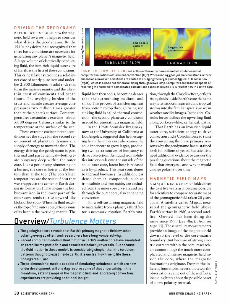
vortices interact with east-west-directed magnetic fields, described as toroidal, that are submerged within the core. These turbulent fluid motions can bend and twist the toroidal field lines into loops called poloidal fields, which have

a north-south orientation. Sometimes the bending is caused by the rising fluid in an upwelling. If the upwelling is strong enough, the top of the poloidal loop is expelled from the core [see box below]. This expulsion creates a pair of

flux patches where the ends of the loop cross the core-mantle boundary. One of these patches has normally directed flux (in the same direction as the overall di-pole field in that hemisphere); the other has the opposite, or reversed, flux.

When the twist causes the reversed flux patch to lie closer to the geograph-ic pole than the normal flux patch, the result is a weakening of the dipole, which is most sensitive to changes near its poles. Indeed, this describes the cur-rent situation with the reversed flux patch below the southern tip of Africa. For an actual planetwide polarity re-versal to occur, such a reversed flux patch would grow and engulf the entire polar region; at the same time, a similar change in overall regional magnetic po-larity would take place near the other geographic pole.

S U P E R C O M P U T E R S I M U L A T I O N Sto f u rt h e r i n v e st ig at e how reversed flux patches develop and how they may signal the onset of the next polarity reversal, researchers simulate the geodynamo on supercomputers and in laboratories. The modern era of com-puter dynamo simulations began in 1995, when three groups—Akira Kageyama of the University of Tokyo and his co-workers; Paul H. Roberts of U.C.L.A. and one of us (Glatzmaier); and Christopher A. Jones of the Univer-sity of Exeter in England and his col-leagues—independently developed nu-merical simulations that generated magnetic fields resembling the magnet-ic field at Earth’s surface. Since then, simulations representing hundreds of thousands of years have demonstrated how convection can indeed produce patches of reversed magnetic flux on the core-mantle boundary—just like those seen in the satellite images. These patch-es come and go in computer simula-tions, but sometimes they lead to spon-taneous magnetic dipole reversals.

Computer-generated polarity rever-sals provided researchers with the first rudimentary glimpse of how such switches may originate and progress [see box on page 34]. One three-dimensional

M A N T L E

O U T E R C O R E

Core-mantle boundary

Reversedflux patch

Reversed magnetic flux

Normal magnetic flux

Helicalcirculation

Toward North Pole

Normalflux patch

a

b

Convective upwelling

R E G I O N S where the direction of magnetic flux is opposite that for the rest of the hemisphere arise when twisted magnetic fields occasionally burst above Earth’s core. These reversed flux patches can weaken the main part of the magnetic field at Earth’s surface, called the dipole, and may even signal the onset of a global polarity reversal. Reversed flux patches originate as fluid rising through the molten outer core pushes upward on roughly horizontal magnetic field lines within the core. This convective upwelling sometimes bends a line until it bulges (a). Earth’s rotation simultaneously drives helical circulation of the molten fluid that can twist the bulge into a loop (b). When the upwelling force is strong enough to expel the loop from the core, a pair of flux patches forms on the core-mantle boundary.

JEN

CH

RIS

TIA

NS

EN

R E V E R S E D F L U X P A T C H E S

32 S C I E N T I F I C A M E R I C A N O U R E V E R C H A N G I N G E A R T H

simulation—which had to run for 12 hours a day every day for more than a year to simulate 300,000 years—de-picted the onset of a reversal as a de-crease in the intensity of the dipole field. Several patches of reversed mag-netic flux, such as those now forming on the core-mantle boundary, then be-gan to appear. But rather than extin-guishing the magnetic field completely, the reversed flux patches created a weak field with a complex mix of polarities during the transition.

Viewed at the surface of the model Earth, the reversal of the dipole oc-curred when the reversed flux patches begin to dominate the original polarity on the core-mantle boundary. In total, it took about 9,000 years for the old po-larity to dissipate and for the new polar-ity to take hold throughout the core.

W H A T M I G H T B E M I S S I N Gbased in pa rt on these successes, computer dynamo models are prolifer-ating rapidly. At last count, more than a dozen groups worldwide were using them to help understand magnetic fields that occur in objects throughout the so-lar system and beyond. But how well do the geodynamo models capture the dy-namo as it actually exists in Earth? The truth is that no one knows for certain.

No computer dynamo model has yet simulated the broad spectrum of turbulence that exists in a planetary in-terior, primarily because massively par-allel supercomputers are not yet fast enough to accurately simulate magnet-ic turbulence with realistic physical pa-rameters in three dimensions. The smallest turbulent eddies and vortices in Earth’s core that twist the magnetic field probably occur on a scale of me-ters to tens of meters, much less than what can be resolved with the current global geodynamo models on the cur-rent supercomputers. That means that all 3-D computer models of the geody-namo so far have simulated the simple, large-scale flow of laminar convection, akin to the hot mineral oil rising through a lava lamp.

To simulate the effects of turbulence in laminar models, investigators have

used unrealistically large values for the fluid viscosity. To achieve realistic tur-bulence in a computer model, research-ers must resort to a two-dimensional

view. The trade-off is that 2-D flow cannot sustain a dynamo. These mod-els do, however, suggest that the lami-nar flows seen in current geodynamo

GARY A. GLATZMAIER and PETER OLSON develop computer models to study the structure and dynamics of the interiors of planets and stars. In the mid-1990s Glatzmaier, then at the Institute of Geophysics and Planetary Physics (IGPP) at Los Alamos National Laboratory, created (together with Paul H. Roberts of the University of California, Los Angeles) the first geodynamo simulation that produced a spontaneous magnetic dipole reversal. Glatzmaier has been a professor in the department of earth sciences and IGPP at the University of California, Santa Cruz, since 1998. Olson is particularly interested in how Earth’s core and mantle interact to produce geomagnetic fields, plate tectonics and deep mantle plumes. He joined the department of earth and planetary sciences at Johns Hopkins University in 1978, where he has introduced geophysics to more than 1,000 students.

THE

AU

THO

RS

1 9 8 0

2 0 0 0

Outward-directed magnetic flux

Increasing intensity

Inward-directed magnetic flux

Increasing intensity

Reversed flux patches

Reversed flux patches

New patches

Enlarged patch

C O N T O U R M A P S of Earth’s magnetic field, extrapolated to the core-mantle boundary from satellite measurements, show that most of the magnetic flux is directed out from the core in the Southern Hemisphere and inward in the Northern Hemisphere. But in a few odd regions, the opposite is true. These so-called reversed flux patches proliferated and grew between 1980 and 2000; if they were to engulf both poles, a polarity reversal could ensue.

PE

TER

OL

SO

N;

SO

UR

CE

: G

AU

THIE

R H

UL

OT

ET

AL

. IN

NAT

UR

E,

VO

L.

41

6,

PA

GE

S 6

20

–6

23

; A

PR

IL 1

1,

20

02

w w w. s c i a m . c o m S C I E N T I F I C A M E R I C A N 33

34 S C I E N T I F I C A M E R I C A N E A R T H S C I E N C E

T H R E E - D I M E N S I O N A L C O M P U T E R simulations of the geodynamo are now capable of producing spontaneous reversals of the magnetic dipole, offering scientists a way to study the origin of reversals preserved in the paleomagnetic record [see timeline on opposite page]. One simulated switch from a model co-developed

by one of us (Glatzmaier) occurred over a 9,000-year interval. This event is depicted as maps of the vertical part of the magnetic field at Earth’s surface and at the core-mantle boundary, where the field is more complex. Models using magnetic field lines provide a third way to visualize a polarity reversal.

M A G N E T I C F I E L D M A P S start off with normal polarity, in which most of the overall magnetic flux points out from the core (yellow) in the Southern Hemisphere and in toward the core (blue) in the Northern Hemisphere (a). The onset of the reversal is marked by several areas of reversed magnetic flux (blue in the south and yellow in the north), reminiscent of the reversed flux patches now forming on Earth’s core-mantle boundary. In about 3,000 years the reversed flux patches have decreased

the intensity of the dipole field until it is replaced by a weaker but complex transition field at the core-mantle boundary (b). The reversal is in full swing by 6,000 years, when the reversed flux patches begin to dominate over the original polarity on the core-mantle boundary (c). If viewed only at the surface, the reversal appears complete by this time. But it takes an additional 3,000 years for the dipole to fully reverse throughout the core (d).

Geographic North

Geographic South

Geographic North

Geographic South

SU

RF

AC

E O

F E

AR

TH

CO

RE

-MA

NT

LE

BO

UN

DA

RY

N O R M A L P O L A R I T Y R E V E R S E D P O L A R I T YP O L A R I T Y R E V E R S A L I N P R O G R E S S

Reversed flux patches

a T I M E = 0 b 3 , 0 0 0 Y E A R S c 6 , 0 0 0 Y E A R S d 9 , 0 0 0 Y E A R S

GA

RY

A.

GL

ATZ

MA

IER

; S

IMU

LA

TED

AT

THE

PIT

TSB

UR

GH

SU

PE

RC

OM

PU

TIN

G C

EN

TER

S I M U L A T E D P O L A R I T Y R E V E R S A L S

b R E V E R S A L I N P R O G R E S S c R E V E R S E D P O L A R I T Ya N O R M A L P O L A R I T Y

C O M P U T E R M O D E L illustrates the magnetic field within the core (tangled lines at center) and the emerging dipole (long

curved lines) 500 years before the middle of a magnetic dipole reversal (a), at the middle (b), and 500 years after that (c).

simulations are much smoother and simpler than the turbulent flows that most likely exist in Earth’s core.

Probably the most significant differ-ence is in the paths the fluid follows as it rises through the core. In simple lam-inar convection simulations, large plumes stretch all the way from the bot-tom of the core to the top. In the turbu-lent 2-D models, on the other hand, convection is marked by multiple small-scale plumes and vortices that detach near the upper and lower boundaries of the core and then interact within the main part of the convection zone.

Such differences in the patterns of fluid flow could have a huge influence on the structure of Earth’s magnetic field and the time it takes various changes to occur. That is why investi-gators are diligently pursuing the next generation of 3-D models. Someday, maybe a decade from now, advances in computer processing speeds will make it possible to produce strongly turbu-lent dynamo simulations. Until then, we hope to learn more from laboratory dynamo experiments now under way.

L A B O R A T O R Y D Y N A M O Sa good way to improve understand-ing of the geodynamo would be to com-pare computer dynamos (which lack turbulence) with laboratory dynamos (which lack convection). Scientists had first demonstrated the feasibility of lab-scale dynamos in the 1960s, but the road to success was long. The vast dif-ference in size between a laboratory ap-paratus and the actual core of a planet was a vital factor. A self-sustaining flu-id dynamo requires that a certain di-mensionless parameter, called the mag-netic Reynolds number, exceed a mini-mum numerical value, roughly 10.

Earth’s core has a large magnetic Reynolds number, probably around

1,000, primarily because it has a large linear dimension (the radius of the core is about 3,485 kilometers). Simply put, it is very difficult to create a large mag-netic Reynolds number in small vol-umes of fluid unless you can move the fluid at extremely high velocities.

The decades-old dream of generat-ing a spontaneous magnetic field in a laboratory fluid dynamo was first real-ized in 2000, when two groups—one led by Agris Gailitis of the University of Latvia and one by Robert Stieglitz and Ulrich Müller of the Karlsruhe Research Center and Fritz Busse of the University of Bayreuth, both in Germany—inde-pendently achieved self-generation in large volumes of liquid sodium. (Liquid sodium was used because of its high electrical conductivity and low melting point.) Both groups found ways to achieve high-speed fluid flow in a sys-tem of one- to two-meter-long helical pipes, resulting in the critical magnetic Reynolds number of about 10.

These experimental results support the theory, which gives us a measure of confidence when we apply our theoreti-cal ideas about dynamos to Earth and other planets. In labs across the world—

at the University of Grenoble in France, the University of Maryland, the Univer-

sity of Wisconsin–Madison and the New Mexico Institute of Mining and Tech-nology—scientists are developing the next generation of lab dynamos. To bet-ter simulate Earth-like geometry, these experiments will stir the liquid sodium inside massive spherical chambers—the largest nearly three meters in diameter.

Besides the ongoing plans for more realistic laboratory dynamos and 3-D computer simulations, the internation-al satellite CHAMP (short for Chal-lenging Minisatellite Payload) is chart-ing the geomagnetic field with enough precision to directly measure its chang-es at the core-mantle boundary in real time. Investigators anticipate this satel-lite will provide a continuous image of the geomagnetic field over its five-year mission, allowing them to watch for continued growth of the reversed flux patches as well as other clues about how the dipole field is waning.

We expect that a synthesis of these three new approaches—satellite obser-vations, computer simulations and lab experiments—will occur in the next de-cade or two. With a more complete pic-ture of the extraordinary geodynamo, we will learn whether our current ideas about the magnetic field and its rever-sals are on the right track.

P O L A R I T Y R E V E R S A L S occurred many times in the past 150 million years and probably long before that as well. Scientists discovered these reversals by studying magnetic minerals. When such a rock cooled long ago, its magnetic field lined up in the direction Earth’s magnetic field at that location and time. The rock retains that ancient magnetic orientation indefinitely, unless it is heated to a temperature high enough to completely remagnetize it.

150 140 130 120 110 100 90 80 70 60 50 40 30 20 10 0

Millions of Years Ago

Normal polarity Reversed polarity Present

JEN

CH

RIS

TIA

NS

EN

; S

OU

RC

E:

D.

V. K

EN

T A

ND

W.

LO

WR

IE I

N T

IME

SC

AL

ES

OF

THE

PA

LE

OM

AG

NE

TIC

FIE

LD

. E

DIT

ED

BY

J.E

.T.

CH

AN

NE

LL

ET

AL

.; A

GU

, 2

00

4

M O R E T O E X P L O R ENumerical Modeling of the Geodynamo: Mechanisms of Field Generation and Equilibration. Peter Olson, Ulrich Christensen and Gary A. Glatzmaier in Journal of Geophysical Research, Vol. 104, No. B5, pages 10383–10404; 1999.

Earth’s Core and the Geodynamo. Bruce A. Buffett in Science, Vol. 288, pages 2007–2012; June 16, 2000.

Geodynamo Simulations: How Realistic Are They? Gary A. Glatzmaier in Annual Review of Earth and Planetary Sciences, Vol. 30, pages 237–257; 2002.

Recent Geodynamo Simulations and Observations of the Geomagnetic Field. Masaru Kono and Paul H. Roberts in Reviews of Geophysics, Vol. 40, No. 4, page 1013; 2002.

w w w. s c i a m . c o m S C I E N T I F I C A M E R I C A N 35