Embed Size (px)
Citation preview

Scientific Computing with Radial Basis
Functions
Edited by
C.S. ChenUniversity of Southern Mississippi, USA
Y.C. HonCity University of Hong Kong, China
R.A. SchabackUniversity of Gottingen, Germany

Contents
page v
Preface vi
1 Introduction 1
1.1 Radial Basis Functions 1
1.2 Multivariate Interpolation and Positive Definiteness 2
1.3 Stability and Scaling 5
1.4 Solving Partial Differential Equations 6
1.5 Comparison of Strong and Weak Problems 7
1.6 Collocation Techniques 9
1.7 Method of Fundamental Solutions 12
1.8 Method of Particular Solutions 13
1.9 Time–dependent Problems 14
1.10 Lists of Radial Basis Functions 14
2 Basic Techniques for Function Recovery 17
2.1 Interpolation of Lagrange Data 17
2.2 Interpolation of Mixed Data 19
2.3 Error Behavior 21
2.4 Stability 22
2.5 Regularization 26
2.6 Scaling 33
2.7 Practical Rules 37
2.8 Large Systems: Computational Complexity 38
2.9 Sensitivity to Noise 41
2.10 Time–dependent Functions 44
3 Collocation Techniques 46
3.1 High Dimensional Problems 47
3.2 Transport Problems 50
iii

iv Contents
3.3 Free Boundary Value Problems 54
3.4 Moving Boundary Value Problems 63
4 The Method of Fundamental Solutions 73
4.1 Introduction 73
4.2 Theoretical Background 75
4.3 Fundamental Solutions 80
4.4 Static Implementation 81
4.5 Interlude: Stability Issues 92
4.6 Dynamic Implementation 102
4.7 Modified Implementation 107
4.8 Special Problems 109
4.9 Inverse Problems 124
5 The Method of Particular Solutions 136
5.1 Introduction 136
5.2 The Dual Reciprocity Method (DRM) 137
5.3 The Method of Particular Solutions (MPS) 138
5.4 Approximate Particular Solutions 139
5.5 Particular Solutions for the Laplace operator 144
5.6 Particular Solutions for Biharmonic Equations 156
5.7 Particular Solutions for Helmholtz Operators 157
5.8 Multiscale Techniques 179
5.9 Solving Large Problems on Circular Points 201
6 Time–Dependent Problems 215
6.1 Method of Laplace Transforms 215
6.2 Time–stepping Methods 220
6.3 Operator-Splitting Methods 232
6.4 Wave Equation 235
References 240
Index 255

This book is dedicated to our families,
as our constant sources of joy and support.
v

Preface
In recent decades radial basis functions have proven to be very useful
in solving problems in Scientific Computing which arise in application
areas like
• Computational Mechanics, including elasticity and stress analysis,
• Fluid dynamics, including shallow water equations, reaction-diffusion
and convection-advection problems,
• Computer Graphics and image analysis, including shape modeling and
animated deformations, and
• Economics, including pricing of options.
These seemingly unrelated applications are linked via certain common
mathematical concepts and problems like
• Recovery of functions from scattered data,
• Meshless methods solving partial differential equations (PDEs),
• Ill–posed and inverse problems,
• Neural networks, and
• Learning algorithms
which can be handled easily and successfully by radial basis functions.
The mathematical reasons for this are covered by books of M.D. Buhmann
[Buh03] and H. Wendland [Wen05] providing the necessary theoretical
background, while a new book of G.E. Fasshauer [Fas07] additionally
covers MATLAB implementations of algorithms.
In contrast to these, this text focuses almost entirely on applications,
with the goal of helping scientists and engineers apply radial basis func-
tions successfully. This book is intended to meet this need. We do not
assume that readers are familiar with the mathematical peculiarities
of radial basis functions. We do, however, assume some knowledge of
vi

Preface vii
the partial differential equations arising in applications, and we include
many computational examples without dealing with implementation is-
sues.
In preparing this text, we soon realized that it was impossible to
cover all of the interesting techniques and applications, as summarized
in a recent Acta Numerica article [SW06]. We decided to leave out
neural networks and kernel-based learning algorithms completely, since
the latter currently supersede the former and are covered in several books
including applications [CST00, SS02, STC04]. Instead we focused on
meshless methods
• for reconstruction of multivariate functions from scattered data, and
• for solving partial differential equations.
Even within these seemingly small areas we had to confine ourselves
to a few core techniques which include Kansa’s method, the method of
fundamental solutions, the method of particular solutions, etc. These
techniques allowed us to extend the radial basis functions to numeri-
cally solving a large class of partial differential equations without mesh
generation. In particular, we devoted a great deal of our effort to the
derivation of particular solutions using radial basis functions for certain
differential operators. Furthermore, this book should enable the reader
to follow the references to other methods not covered here and to keep
up with the pace of new developments in the area. To this end, we
included some unpublished material at various places.
This manuscript has been used as lecture notes to teach at the grad-
uate special topic courses in scientific computing at the University of
Nevada, Las Vegas (UNLV) during 2004–2005 and the University of
Southern Mississippi (USM) during 2006–2007. During the course of
teaching these classes, we have been fortunate that our students have
enthusiastically given us a great amount of feedback and have allowed
us to constantly make revision of the content of the book. It is worth
mentioning that, due to these courses, two Master’s theses in meshless
methods were produced at UNLV and two potential Ph.D. theses in a
similar topic at USM are currently being done. We are pleased to see
some of our students were able to adopt new concepts they learn from
the book, and had turned them into research projects, and presenting
their results in conferences and conference proceedings. As such, we be-
lieve the book is suitable for a one year graduate or post-graduate course
in the area of scientific computing.
viii Preface
We would like to acknowledge the editorial help from Drs. John Dud-
ley and Joseph Kolibal at USM. We also appreciate Dr. Michael Golberg,
and Professor Andreas Karageorghis and Professor Greame Fairweather
for providing important references in the method of fundamental solu-
tions. The comments and suggestions from Professor Karageorghis to
improve our book is especially helpful. Part of this monograph was com-
pleted during the course of Dr. Chen’s summer visit in 2004 to Professor
Satya Atluri at the University of California, Irvine. The kind support of
Professor Atluri is greatly appreciated. The institutional support from
the University of Southern Mississippi, City University of Hong Kong,
and the University of Gottingen for providing resources and facilities to
complete this project is also critical and we would like to express our
gratitude for this support.
September 11, 2007 C.S. Chen, Y.C. Hon, and R.A. Schaback

1
Introduction
1.1 Radial Basis Functions
Scientific Computing with Radial Basis Functions focuses on the recovery
of unknown functions from known data. The functions are multivariate
in general, and they may be solutions of partial differential equations
satisfying certain additional conditions. However, the reconstruction
of multivariate functions from data may cause problems if the space
furnishing the “trial” functions is not fixed in advance, but is data–
dependent [Mai56]. Finite elements (see e.g. [Bra01, BS02]) provide
such data–dependent spaces. They are defined as piecewise polynomial
functions on regular triangularizations.
To avoid triangularizations, re-meshing and other geometric program-
ming efforts, meshless methods have been suggested [BKO+96]. This
book focuses on a special class of meshless techniques for generating
data–dependent spaces of multivariate functions. The spaces are spanned
by shifted and scaled instances of radial basis functions (RBF) like
the multiquadric [Har71]
x 7→ Φ(x) :=√
1 + ‖x‖22, x ∈ IRd
or the Gaussian
x 7→ Φ(x) := exp(−‖x‖22), x ∈ IRd.
These functions are multivariate, but reduce to a scalar function of the
Euclidean norm ‖x‖2 of their vector argument x, i.e. they are radial in
the sense
Φ(x) = φ(‖x‖2) = φ(r), x ∈ IRd
for the “radius” r = ‖x‖2 with a scalar function φ : IR → IR. This
1

2
makes their use for high–dimensional reconstruction problems very effi-
cient, and it induces invariance under orthogonal transformations.
Recovery of functions from meshless data is then made by trial func-
tions u which are linear combinations
u(x) :=n∑
k=1
αkφ(‖x − yk‖2) (1.1.1)
of translates φ(‖x − yk‖2) of a single radial basis function. The trans-
lations are specified by vectors y1, . . . ,yn of IRd, sometimes called cen-
ters or trial points, without any special assumptions on their number
or geometric position. This is why the methods of this book are truly
“meshless.” In certain cases one has to add multivariate polynomials in
x to the linear combinations in (1.1.1), but we postpone these details.
Our main goal is to show how useful radial basis functions are in appli-
cations, in particular for solving partial differential equations (PDE) of
science and engineering. Therefore we keep the theoretical background
to a minimum, referring to recent books [Buh03, Wen05, Fas07] on ra-
dial basis functions whenever possible. Furthermore, we have to ignore
generalizations of radial basis functions to kernels. These arise in many
places, including probability and learning theory, and they are surveyed
in [SW06]. The rest of this chapter gives an overview of the applications
we cover in this book.
1.2 Multivariate Interpolation and Positive Definiteness
The simplest case of reconstruction of a d–variate unknown function u∗
from data occurs when only a finite number of data in the form of val-
ues u∗(x1), . . . , u∗(xm) at arbitrary locations x1, . . . ,xm in IRd forming
a set X := x1, . . . ,xm are known. In contrast to the n trial cen-
ters y1, . . . ,yn of (1.1.1), the m data locations x1, . . . ,xm are called
test points or collocation points in later applications. To calcu-
late a trial function u of the form (1.1.1) which reproduces the data
u∗(x1), . . . , u∗(xm) well, we have to solve the m× n linear system
n∑
k=1
αkφ(‖xi − yk‖2) ≈ u∗(xi), 1 ≤ i ≤ m (1.2.1)
for the n coefficients α1, . . . , αn. Matrices with entries φ(‖xi−yk‖2) will
occur at many places in the book, and they are called kernel matrices
in machine learning.
Of course, users will usually make sure that m ≥ n holds by picking at

Introduction 3
least as many test points as trial centers, but the easiest case will occur
when the centers yk of trial functions (1.1.1) are chosen to be identical
to the data locations xj for 1 ≤ j ≤ m = n. If there is no noise in the
data, it then makes sense to reconstruct u∗ by a function u of the form
(1.1.1) by enforcing the exact interpolation conditions
u∗(xj) =
n∑
k=1
αjφ(‖xj − xk‖2), 1 ≤ j ≤ m = n. (1.2.2)
This is a system of m linear equations in n = m unknowns α1, . . . , αn
with a symmetric kernel matrix
AX := (φ(‖xj − xk‖2))1≤j,k≤m (1.2.3)
In general, solvability of such a system is a serious problem, but one of
the central features of kernels and radial basis functions is to make this
problem obsolete via
Definition 1.2.4 A radial basis function φ on [0,∞) is positive defi-
nite on IRd, if for all choices of sets X := x1, . . . ,xm of finitely many
points x1, . . . ,xm ∈ IRd and arbitrary m the symmetric m×m matrices
AX of (1.2.3) are positive definite.
Consequently, solvability of the system (1.2.2) is guaranteed if φ satis-
fies the above definition. This holds for several standard radial basis
functions provided in Table 1.1, but users must be aware that problems
may occur when using other scalar functions such as exp(−r). A more
detailed list of radial basis functions will follow later on page 15.
Name φ(r)
Gaussian exp(−r2)
Inverse multiquadrics (1 + r2)β/2, β < 0
Matern/Sobolev Kν(r)rν , ν > 0
Table 1.1. Positive definite radial basis functions
But there are some very useful radial basis functions which fail to be
positive definite. In such cases one has to add polynomials of a certain
maximal degree to the trial functions of (1.1.1). Let P dQ−1 denote the
space spanned by all d-variate polynomials of degree up to Q − 1, and
pick a basis p1, . . . , pq of this space. The dimension q then comes out to

4
be q =(Q−1+d
d
), and the trial functions of (1.1.1) are augmented to
u(x) :=
n∑
k=1
αkφ(‖x − yk‖2) +
q∑
ℓ=1
βℓpℓ(x). (1.2.5)
Now there are q additional degrees of freedom, but these are removed
by q additional homogeneous equations
n∑
k=1
αkpℓ(xk) = 0, 1 ≤ ℓ ≤ q (1.2.6)
restricting the coefficients α1, . . . , αn in (1.2.5). Unique solvability of
the extended system
n∑
k=1
αkφ(‖xj − yk‖2) +
q∑
ℓ=1
βℓpℓ(xj) = u(xj), 1 ≤ j ≤ n
n∑
k=1
αkpℓ(xk) = 0, 1 ≤ ℓ ≤ q
(1.2.7)
is assured if
p(xk) = 0 for all 1 ≤ k ≤ n and p ∈ P dQ−1 implies p = 0. (1.2.8)
This is the proper setting for conditionally positive definite radial
basis functions of order Q, and in case Q = 0 it will coincide with what
we had before, since then q = 0 holds, (1.2.6) is empty, and (1.2.5) re-
duces to (1.1.1). We leave details of this to the next chapter, but we
want the reader to be aware of the necessity of adding polynomials in
certain cases. Table 1.2 provides a selection of the most useful condi-
tionally positive definite functions, and again we refer to Table 1.3 on
page 15 for other radial basis functions.
Name φ(r) Q condition
multiquadric (−1)⌈β/2⌉(1 + r2)β/2 ⌈β/2⌉ β > 0, β /∈ 2IN
polyharmonic (−1)⌈β/2⌉rβ ⌈β/2⌉ β > 0, β /∈ 2IN
polyharmonic (−1)1+β/2rβ log r 1 + β/2 β > 0, β ∈ 2IN
thin–plate spline r2 log r 2
Table 1.2. Conditionally positive definite radial basis functions

Introduction 5
1.3 Stability and Scaling
Solving the system (1.2.2) is easy to program, and it is always possible
if φ is a positive definite radial basis function. But it also can cause
practical problems, since it may be badly conditioned and is non–sparse
in case of globally non–vanishing radial basis functions. To handle bad
conditions of moderately large systems, one can rescale the radial basis
function used, or one can calculate an approximate solution by solving a
properly chosen subsystem. Certain decomposition and preconditioning
techniques are also possible, but details will be postponed to the next
chapter.
In absence of noise, systems of the form (1.2.2) or (1.2.7) will in most
cases have a very good approximate solution, because the unknown
function u providing the right-hand side data can usually be well ap-
proximated by the trial functions used in (1.1.1) or (1.2.5). This means
that even for high condition numbers there is a good reproduction of the
right-hand side by a linear combination of the columns of the matrix.
The coefficients are in many cases not very interesting, since users want
to have a good trial function recovering the data well, whatever the co-
efficients are. Thus users can apply specific numerical techniques like
singular value decomposition or optimization algorithms to get
useful results in spite of bad conditions. We shall supply details in the
next chapter, but we advise users not to use primitive solution methods
for their linear systems.
For extremely large systems, different techniques are necessary. Even
if a solution can be calculated, the evaluation of u(x) in (1.1.1) at
a single point x has O(n) complexity, which is not tolerable in gen-
eral. This is why some localization is necessary, cutting the evaluation
complexity at x down to O(1). At the same time, such a localization
will make the system matrix sparse, and efficient solution techniques
like preconditioned conjugate gradients become available. Finite ele-
ments achieve this by using a localized basis, and the same method
also works for radial basis functions, if scaled functions with compact
support are used. Fortunately, positive definite radial functions with
compact support exist for all space dimensions and smoothness require-
ments [Wu95, Wen95, Buh98]. The most useful example is Wendland’s
function
φ(r) =
(1 − r)4(1 + 4r), 0 ≤ r ≤ 1,
0, r ≥ 1,
which is positive definite in IRd for d ≤ 3 and twice differentiable in x

6
when r = ‖x‖2 (see Table 1.1 and other cases in Table 1.3 on page 15).
Other localization techniques use fast multipole methods [BGP96,
BG97] or a partition of unity [Wen02]. This technique originated from
finite elements [MB96, BM97], where it served to patch local finite
element systems together. It superimposes local systems in general,
using smooth weight functions, and thus it also works well if the local
systems are made up using radial basis functions.
However, all localization techniques require some additional geometric
information, e.g. a list of centers yk which are close to any given point
x. Thus the elimination of triangulations will, in case of huge systems,
bring problems of Computational Geometry through the back door.
A particularly local interpolation technique, which does not solve any
system of equations but can be efficiently used for any local function
reconstruction process, is the method of moving least squares [LS81,
Lev98, Wen01]. We have to ignore it here. Chapter 2 will deal with
radial basis function methods for interpolation and approximation in
quite some detail, including methods for solving large systems in Section
2.8.
1.4 Solving Partial Differential Equations
With some modifications, the above observations will carry over to solv-
ing partial differential equations. In this introduction, we confine our-
selves to a Poisson problem on a bounded domain Ω ⊂ IR3 with a
reasonably smooth boundary ∂Ω. It serves as a model case for more
general partial differential equations of science and engineering that we
have in mind. If functions fΩ on the domain Ω and fΓ on the boundary
Γ := ∂Ω are given, a function u on Ω ∪ Γ with
−∆u = fΩ in Ω
u = fΓ in Γ(1.4.1)
is to be constructed, where ∆ is the Laplace operator
∆u =∂2u
∂x21
+∂2u
∂x22
+∂2u
∂x23
in Cartesian coordinates x = (x1, x2, x3)T ∈ IR3. This way the prob-
lem is completely posed in terms of evaluations of functions and deriva-
tives, without any integrations. However, this requires taking second
derivatives of u, and a careful mathematical analysis shows that there
are cases where this assumption is questionable. It holds only under

Introduction 7
certain additional assumptions, and this is why the above formulation is
called a strong form. Except for the next section, we shall deal exclu-
sively with methods for solving partial differential equations in strong
form.
A weak form is obtained by multiplication of the differential equation
by a smooth test function v with compact support within the domain
Ω. Using Green’s formula (a generalization of integration by parts), this
converts to
−∫
Ω
v · (∆u∗)dx =
∫
Ω
v · fΩdx
︸ ︷︷ ︸=:(v,fΩ)L2(Ω)
=
∫
Ω
(∇v) · (∇u∗)dx︸ ︷︷ ︸
=:a(v,u∗)
or, in shorthand notation, to an infinite number of equations
a(v, u∗) = (v, fΩ)L2(Ω) for all test functions v
between two bilinear forms, involving two local integrations. This tech-
nique gets rid of the second derivative, at the cost of local integration,
but with certain theoretical advantages we do not want to explain here.
1.5 Comparison of Strong and Weak Problems
Concerning the range of partial differential equation techniques we han-
dle in this book, we restrict ourselves to cases we can solve without
integrations, using radial basis functions as trial functions. This im-
plies that we ignore boundary integral equation methods and finite el-
ements as numerical techniques. For these, there are enough books on
the market. Since there is no integration, we need no “background” or
“integration” mesh, and some authors call such methods “truly mesh-
less”.
On the analytical side, we shall consider only problems in strong
form, i.e. where all functions and their required derivatives can be eval-
uated pointwise. Some readers might argue that this rules out too many
important problems. Therefore we want to provide some arguments in
favor of our choice. Readers without a solid mathematical background
should skip over these remarks.
First, we do not consider the additional regularity needed for a strong
solution to be a serious drawback in practice. Useful error bounds and
rapidly convergent methods will always need regularity assumptions on
the problem and its solutions. Thus our techniques should be compared
to spectral methods or the p–technique in finite elements. If a solution

8
of a weak Poisson problem definitely is not a solution of a strong problem,
the standard finite element methods will not converge with reasonable
orders anyway, and we do not want to compete in such a situation.
Second, the problems to be expected from taking a strong form instead
of a weak form can in many cases be eliminated. To this end, we look
at those problems somewhat more closely.
The first case comes from domains with incoming corners. Even if
the data functions fΩ and fΓ are smooth, there may be a singularity of
u∗ at the boundary. However, this singularity is a known function of the
incoming corner angle, and by adding an appropriate function to the set
of trial functions, the problem can be overcome.
The next problem source is induced by non–smooth data functions.
Since these are fixed, the exceptional points are known in principle, and
precautions can be taken by using nonsmooth trial functions with sin-
gularities located properly. For time–dependent problems with moving
boundaries or discontinuities, meshless methods can be adapted very
flexibly, but this is a research area which is beyond the scope of this
book.
The case of data functions which do not allow point evaluations (i.e.
fΩ ∈ L2(Ω) or even distributional data for the Poisson problem) and
still require integration can be ruled out too, because on the one hand
we do not know a single case from applications, and on the other hand
we would like to know how to handle this case with a standard finite
element code, which usually integrates by applying integration formulae.
The latter can never work for L2 functions.
Things are fundamentally different when applications in science or
engineering insist on distributional data. Then weak forms are un-
avoidable, and we address this situation now.
Many of the techniques here can be transferred to weak forms, if
absolutely necessary. This is explained to some extent in [HS05] for
a class of symmetric meshless methods. The meshless local Petrov–
Galerkin (MLPG) method [AZ98a, AZ98b, AZ00] of S.N. Atluri and
collaborators is a good working example of a weak meshless technique
with plenty of successful applications in engineering, Because it is both
weak and unsymmetric, its mathematical analysis is hard, and thus it
only recently was put on a solid theoretical foundation [Sch06c].
Finally, mixed weak and strong problems are possible [HS05, Sch06c],
confining the weak approach to areas where severe regularity problems
occur or data are distributional. Together with adaptivity, mixed meth-
ods will surely prove useful in the future.
Introduction 9
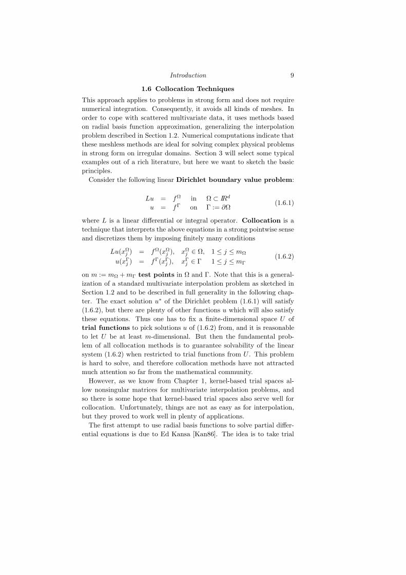
1.6 Collocation Techniques
This approach applies to problems in strong form and does not require
numerical integration. Consequently, it avoids all kinds of meshes. In
order to cope with scattered multivariate data, it uses methods based
on radial basis function approximation, generalizing the interpolation
problem described in Section 1.2. Numerical computations indicate that
these meshless methods are ideal for solving complex physical problems
in strong form on irregular domains. Section 3 will select some typical
examples out of a rich literature, but here we want to sketch the basic
principles.
Consider the following linear Dirichlet boundary value problem:
Lu = fΩ in Ω ⊂ IRd
u = fΓ on Γ := ∂Ω(1.6.1)
where L is a linear differential or integral operator. Collocation is a
technique that interprets the above equations in a strong pointwise sense
and discretizes them by imposing finitely many conditions
Lu(xΩj ) = fΩ(xΩ
j ), xΩj ∈ Ω, 1 ≤ j ≤ mΩ
u(xΓj ) = fΓ(xΓ
j ), xΓj ∈ Γ 1 ≤ j ≤ mΓ
(1.6.2)
on m := mΩ +mΓ test points in Ω and Γ. Note that this is a general-
ization of a standard multivariate interpolation problem as sketched in
Section 1.2 and to be described in full generality in the following chap-
ter. The exact solution u∗ of the Dirichlet problem (1.6.1) will satisfy
(1.6.2), but there are plenty of other functions u which will also satisfy
these equations. Thus one has to fix a finite-dimensional space U of
trial functions to pick solutions u of (1.6.2) from, and it is reasonable
to let U be at least m-dimensional. But then the fundamental prob-
lem of all collocation methods is to guarantee solvability of the linear
system (1.6.2) when restricted to trial functions from U . This problem
is hard to solve, and therefore collocation methods have not attracted
much attention so far from the mathematical community.
However, as we know from Chapter 1, kernel-based trial spaces al-
low nonsingular matrices for multivariate interpolation problems, and
so there is some hope that kernel-based trial spaces also serve well for
collocation. Unfortunately, things are not as easy as for interpolation,
but they proved to work well in plenty of applications.
The first attempt to use radial basis functions to solve partial differ-
ential equations is due to Ed Kansa [Kan86]. The idea is to take trial

10
functions of the form (1.1.1) or (1.2.5), depending on the order of the
positive definiteness of the radial basis function used. For positive q one
also has to postulate (1.2.6), and thus one should take n := m + q to
arrive at a problem with the correct degrees of freedom. The collocation
equations come out in general as
n∑
k=1
αk∆φ(‖xΩj − yk‖2) +
q∑
ℓ=1
βℓ∆pℓ(xΩj ) = fΩ(xΩ
j ), 1 ≤ j ≤ mΩ
n∑
k=1
αkφ(‖xΓj − yk‖2) +
q∑
ℓ=1
βℓpℓ(xΓj ) = fΓ(xΓ
j ), 1 ≤ j ≤ mΓ
n∑
k=1
αkpℓ(yk) + 0 = 0, 1 ≤ ℓ ≤ q,
(1.6.3)
forming a linear unsymmetric n× n = (mΩ +mΓ + q)× (mΩ +mΓ + q)
system of equations. In all known applications, the system is nonsingu-
lar, but there are specially constructed cases [HS01] where the problem
is singular.
A variety of experimental studies, e.g. by Kansa [Kan90a, Kan90b],
Golberg and Chen [GCK96], demonstrated this technique to be very
useful for solving partial differential and integral equations in strong
form. Hon et. al. further extended the applications to the numeri-
cal solutions of various ordinary and partial differential equations in-
cluding general initial value problems [HM97], the nonlinear Burgers
equation with a shock wave [HM98], the shallow water equation
for tide and current simulation in domains with irregular boundaries
[Hon93], and free boundary problems like the American option
pricing [HM99, Hon02]. These cases will be reported in Chapter 3.
Due to the unsymmetry, the theoretical possibility of degeneration, and
the lack of a seminorm-minimization in the analytic background, a the-
oretical justification is difficult but was provided recently [Sch07b] for
certain variations of the basic approach.
The lack of symmetry may be viewed as a bug, but it also can be
seen as a feature. In particular, the method does not assume ellipticity
or self-adjointness of differential operators. Thus it applies to a very
general class of problems, as many applications show.
On the other hand, symmetry can be brought back again by a suitable
change of the trial space. In the original method, there is no connection
between the test points xΩj , xΓ
j and the trial centers yk. If the trial
points are dropped completely, one can recycle the test points to define

Introduction 11
new trial functions by
u(x) :=
mΩ∑
i=1
αΩi ∆φ(‖x−xΩ
i ‖2)+
mΓ∑
j=1
αΓj φ(‖x−xΓ
j ‖2)+
q∑
ℓ=1
βℓpℓ(x) (1.6.4)
providing the correct number n := mΩ +mΓ + q of degrees of freedom.
Note how the test points xΩi and xΓ
j lead to different kinds of trial
functions, since they apply “their” differential or boundary operator to
one of the arguments of the radial basis function.
The collocation equations now come out as a symmetric square linear
system with block structure. If we define vectors
fΩ := (fΩ(xΩ1 ), . . . , fΩ(xΩ
mΩ))T ∈ IRmΩ
fΓ := (fΓ(xΓ1 ), . . . , fΓ(xΓ
mΓ))T ∈ IRmΓ
0q := (0, . . . , 0)T ∈ IRq
aΩ := (αΩ1 , . . . , α
ΩmΩ
)T ∈ IRmΩ
aΓ := (αΓ1 , . . . , α
ΓmΓ
)T ∈ IRmΓ
bq := (β1, . . . , βq)T ∈ IRq,
we can write the system with a slight abuse of notation as
∆2φ(‖xΩr − xΩ
i ‖2) ∆φ(‖xΩr − xΓ
j ‖2) ∆pℓ(xΩr )
∆φ(‖xΓs − xΩ
i ‖2) φ(‖xΓs − xΓ
j ‖2) pℓ(xΓs )
∆pt(xΩi ) pt(x
Γj ) 0
aΩ
aΓ
bq
=
fΩ
fΓ
0q
where indices in the submatrices run over
1 ≤ i, r ≤ mΩ
1 ≤ j, s ≤ mΓ
1 ≤ ℓ, t ≤ q.
The first set of equations arises when applying ∆ to (1.6.4) on the domain
test points xΩr . The second is the evaluation of (1.6.4) on the boundary
test points xΓs . The third is a natural generalization of (1.2.6) to the
current trial space. Note that the system has the general symmetric
form
AΩ,Ω AΩ,Γ PΩ
AΩ,ΓTAΓ,Γ PΓ
PΩTPΓT
0q×q
aΩ
aΓ
bq
=
fΩ
fΓ
0q
(1.6.5)
with evident notation when compared to the previous display.
Under weak assumptions, such matrices are nonsingular [Wu92, Isk95]
because they arise as Hermite interpolation systems generalizing (1.2.2).
The approach is called symmetric collocation and has a solid math-
ematical foundation [FS98b, FS98a] making use of the symmetry of the

12
discretized problem. We provide specific applications in Chapter 3 and
some underlying theory in Section 2.2.
1.7 Method of Fundamental Solutions
This method is a highly effective technique for solving homogeneous
differential equations, e.g. the potential problem (1.4.1) with fΩ = 0.
The basic idea is to use trial functions that satisfy the differential equa-
tion and to superimpose the trial functions in such a way that the ad-
ditional boundary conditions are satisfied with sufficient accuracy. It
reduces a homogeneous partial differential equation problem to an ap-
proximation or interpolation problem on the boundary by fitting the
data on the boundary. Since fundamental solutions are special homoge-
neous solutions which are well-known and easy to implement for many
practically important differential operators, the method of fundamental
solutions is a relatively easy way to find the desired solution of a given
homogeneous differential equation with the correct boundary values.
For example, the function uy(x) := ‖x− y‖−12 satisfies (∆uy)(x) = 0
everywhere in IR3 except for x = y, where it is singular. But if points
y1, . . . ,yn are placed outside the domain Ω, any linear combination u
of the uy1 , . . . , uynwill satisfy ∆u = 0 on all of Ω. Now the freedom
in the coefficients can be used to make u a good approximation to fΓ
on the boundary. For this, several methods are possible, but we do not
want to provide details here. It suffices to see that we have got rid of
the differential equation, arriving at a plain approximation problem on
the boundary of Ω.
The method of fundamental solutions was first proposed by Kupradze
and Aleksidze [KA64b] in 1964. During the past decades, the method
has re-emerged as a popular boundary-type meshless method and has
been applied to solve various science and engineering problems. One
of the reasons for the renewed interest for this method is that it has
been successfully extended to solve inhomogeneous and time–dependent
problems. As a result, the method now is applicable to a larger class of
partial differential equations. Furthermore, it does not require numerical
integration and is “truly meshless” in the sense that no tedious domain
or boundary mesh is necessary. Hence the method is extremely simple
to implement, making it especially attractive to scientists and engineers
working in applications.
In many cases, e.g. for the potential equation, the underlying math-
ematical analysis has a maximum principle [PW67, Jos02] for homo-
Introduction 13
geneous solutions, and then the total error is bounded by the error on
the boundary, which can be evaluated easily. Furthermore, adaptive
versions are possible, introducing more trial functions to handle places
where the boundary error is not tolerable. In very restricted cases, con-
vergence of these methods can be proven to be spectral (i.e. faster than
any fixed order), and for “smooth” application problems this technique
shows an extremely good convergence behavior in practice.
This book is the first to give a comprehensive treatment of the method
of fundamental solutions (MFS). The connection to radial basis func-
tion techniques is that fundamental solutions of radially invariant dif-
ferential operators like the Laplace or the Helmholtz operator have ra-
dial form around a singularity, as in the above case. For example, one
of the most widely used radial basis functions, the thin–plate spline
φ(r) := r2 log r is the fundamental solution at the origin to the thin–
plate equation ∆2u = 0 in IR2.
Methods which solve homogeneous equations by superposition of gen-
eral solutions and an approximation on the boundary have quite some
history, dating back to Trefftz [Tre26]. In particular, the work of L. Col-
latz [MNRW91] contains plenty of examples done in the 1960’s. Later,
this subject was taken up again and called Boundary Knot Method
[CT00, Che02, CH03, HC03], but we stick to the Method of Fundamen-
tal Solutions here. A recent technique [Sch07c] for solving homogeneous
problems is based on singularity–free kernels. It has a full mathematical
background theory, but is still rather special and under investigation.
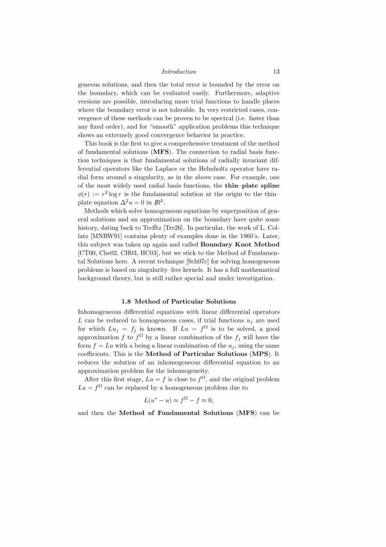
1.8 Method of Particular Solutions
Inhomogeneous differential equations with linear differential operators
L can be reduced to homogeneous cases, if trial functions uj are used
for which Luj = fj is known. If Lu = fΩ is to be solved, a good
approximation f to fΩ by a linear combination of the fj will have the
form f = Lu with u being a linear combination of the uj , using the same
coefficients. This is the Method of Particular Solutions (MPS). It
reduces the solution of an inhomogeneous differential equation to an
approximation problem for the inhomogeneity.
After this first stage, Lu = f is close to fΩ, and the original problem
Lu = fΩ can be replaced by a homogeneous problem due to
L(u∗ − u) ≈ fΩ − f ≈ 0,
and then the Method of Fundamental Solutions (MFS) can be

14
applied. The approximation of fΩ by f can be done by interpolation or
approximation techniques of the previous sections, provided that the fj
are translates of radial basis functions.
Inhom. PDEMPS⇒
App. in interior
Homog. PDEMFS⇒ App. on boundary
This is how the major techniques of this book are related. For the most
important differential operators and radial basis functions, we provide
useful (uj, fj) pairs with Luj = fj and show their applications.
1.9 Time–dependent Problems
In the final chapter, we extend the method of fundamental solutions and
the method of particular solutions to solving time–dependent problems.
A common feature of the methods in this chapter is that a given time–
dependent problem is reduced to an inhomogeneous modified Helmholtz
equation through the use of two basic techniques:
• Laplace transforms and
• time–stepping algorithms.
Using the Laplace transform, the given time–dependent problem can be
solved in one step in Laplace space and then converted back to the orig-
inal time space using the inverse Laplace transform. By time-stepping,
the given time–dependent problem is transformed into a sequence of
modified Helmholtz equations which in turn can be solved by the nu-
merical procedures described in the previous chapters. In the parabolic
case, we consider both linear and nonlinear heat equations. In the hyper-
bolic case, we only consider the wave equation using the time-stepping
algorithm. Readers are encouraged to apply this approach to solve more
challenging time–dependent problems.
1.10 Lists of Radial Basis Functions
Table 1.3 shows a selection of the most popular radial basis functions
φ(r) with non–compact support. We provide the minimal order Q of
conditional positive definiteness and indicate the range of additional
parameters.
Classes of compactly supported radial basis functions were pro-
vided by Wu [Wu95], Wendland [Wen95], and Buhmann [Buh98]. We list

Introduction 15
Name φ(r) Q condition
Gaussian exp(−r2) 0
Matern rνKν(r) 0 ν > 0
inverse multiquadric (1 + r2)β/2 0 β < 0
multiquadric (−1)⌈β/2⌉(1 + r2)β/2 ⌈β/2⌉ β > 0, β /∈ 2IN
polyharmonic (−1)⌈β/2⌉rβ ⌈β/2⌉ β > 0, β /∈ 2IN
polyharmonic (−1)1+β/2rβ log r 1 + β/2 β > 0, β ∈ 2IN
Table 1.3. Global RBFs
a selection of Wendland’s functions in Table 1.4. These are always pos-
itive definite up to a maximal space dimension dmax, and have smooth-
ness Ck as indicated in the table. Their polynomial degree is minimal for
given smoothness, and they have a close connection to certain Sobolev
spaces.
φ(r) k dmax
(1 − r)2+ 0 3
(1 − r)4+(4r + 1) 2 3
(1 − r)6+(35r2 + 18r + 3) 4 3
(1 − r)8+(32r3 + 25r2 + 8r + 1) 6 3
(1 − r)3+ 0 5
(1 − r)5+(5r + 1) 2 5
(1 − r)7+(16r2 + 7r + 1) 4 5
Table 1.4. Selection of Wendland’s compactly supported radial basis
functions

16
−2 −1.5 −1 −0.5 0 0.5 1 1.5 2−0.5
0
0.5
1
1.5
2
2.5
3
Gauss
Wendland C2
Thin−plate spline
Inverse Multiquadric
Multiquadric
Fig. 1.1. Some radial basis functions

2
Basic Techniques for Function Recovery
This chapter treats a basic problem of Scientific Computing: the recov-
ery of multivariate functions from discrete data. We shall use radial
basis functions for this purpose, and we shall confine ourselves to re-
construction from strong data consisting of evaluations of the function
itself or its derivatives at discrete points. Recovery of functions from
weak data, i.e. from data given as integrals against test functions, is a
challenging research problem [Sch06b, Sch06c], but it has to be ignored
here. Note that weak data require integration, and we want to avoid
unnecessary background meshes used for this purpose.
2.1 Interpolation of Lagrange Data
Going back to Section 1.2, we assume data values y1, . . . , ym ∈ IR to be
given, which are supposed to be values yk = u∗(xk) of some unknown
function u∗ at scattered points x1, . . . ,xm in some domain Ω in IRd. We
then pick a positive definite radial basis function φ and set up the linear
system (1.2.2) of m equations for the m coefficients α1, . . . , αm of the
representation (1.1.1) where n = m and yk = xk for all k. In case of
conditionally positive radial basis functions, we have to use (1.2.5) and
add the conditions (1.2.6).
In Figure 2.1 we have 150 scattered data points in [−3, 3]2 in which
we interpolate the MATLAB peaks function (top right). The next row
shows the interpolant using Gaussians and the absolute error. The lower
row shows MATLAB’s standard technique for interpolation of scattered
data using the griddata command. The results are typical for such
problems: radial basis function interpolants recover smooth functions
very well from a sample of scattered values, provided that the values are
noiseless and the underlying function is smooth.
17

18
Fig. 2.1. Interpolation by radial basis functions
The ability of radial basis functions to deal with arbitrary point lo-
cations in arbitrary dimensions is very useful when geometrical objects
have to be constructed, parametrized, or warped, see e.g. [ADR94,
CFB97, NFN00, CBC+01, OBS03, RTSD03, WK05, BK05]. In par-
ticular, one can use such transformations to couple incompatible finite
element codes [ABW06].
Furthermore, interpolation of functions has quite some impact on
methods solving partial differential equations. In Chapter 5 we shall
solve inhomogeneous partial differential equations by interpolating the
right-hand sides by radial basis functions which are related to particular
solutions of the partial differential equation in question.
Another important issue is the possibility parametrizing spaces of
translates of kernels not via coefficients, but via function values at the
translation centers. This simplifies meshless methods “constructing
the approximation entirely in terms of nodes” [BKO+96]. Since kernel
interpolants approximate higher derivatives well, local function values
can be used to provide good estimates for derivative data [WHW05].
This has connections to pseudospectral methods [Fas04].

Basic Techniques for Function Recovery 19
2.2 Interpolation of Mixed Data
It is quite easy to allow much more general data for interpolation by
radial basis functions. For example, consider recovery of a multivariate
function f from data including the values ∂f∂x2
(z),∫Ω f(t)dt. The basic
trick, due to Z.M. Wu [Wu92], is to use special trial functions
∂φ(‖x − z‖2)
∂x2for
∂f
∂x2(z)
∫
Ω
φ(‖x − t‖2)dt for
∫
Ω
f(t)dt
to cope with these requirements. In general, if a linear functional λ
defines a data value λ(f) for a function f as in the above cases with
λ1(f) = ∂f∂x2
(z), λ2(f) =∫Ω f(t)dt, the special trial function uλ(x) to
be added is
uλ(x) := λtφ(‖x − t‖2) for λt(f(t))
where the upper index denotes the variable the functional acts on. If
m = n functionals λ1, . . . , λm are given, the span (1.1.1) of trial functions
is to be replaced by
u(x) =n∑
k=1
αkλtkφ(‖x − t‖2).
The interpolation system (1.2.2) turns into
λju =n∑
k=1
αkλtkλ
xj φ(‖x − t‖2), 1 ≤ j ≤ n (2.2.1)
with a symmetric matrix composed of λtkλ
xj φ(‖x − t‖2), 1 ≤ j, k ≤
n which is positive definite if the functionals are linearly independent
and φ is positive definite. Thus a fully general Hermite–Birkhoff
interpolation is possible as long as the entries of the matrix in (2.2.1)
are meaningful.
To give an example with general functionals, Figure 2.2 shows an
interpolation to Neumann data +1 and -1 on each half of the unit circle,
respectively, in a total of 64 points by linear combinations of properly
scaled Gaussians.
In case of conditionally positive definite radial basis functions, the
span of (1.2.5) turns into
u(x) :=
n∑
k=1
αkλtkφ(‖x − t‖2) +
q∑
ℓ=1
βℓpℓ(x)

20
−1
−0.5
0
0.5
1
−1
−0.5
0
0.5
1
−4
−3
−2
−1
0
1
2
3
4
x 104
Fig. 2.2. Generalized interpolant to Neumann data
while the additional condition (1.2.6) is replaced by
n∑
k=1
αkλtkpℓ(t) = 0, 1 ≤ ℓ ≤ q,
and the interpolation problem is solvable, if the standard polynomial
unisolvency constraint
λtkp(t) = 0 for all 1 ≤ k ≤ n and p ∈ P d
Q−1 implies p = 0
is imposed, replacing (1.2.8).
Another example of recovery from non–Lagrange data is the construc-
tion of Lyapounov basins from data consisting of orbital derivatives
[GW06a, GW06b].
The flexibility to cope with general data is the key to various applica-
tions of radial basis functions within methods solving partial differential
equations. Collocation techniques, as sketched in Section 1.6 and treated
in Chapter 3 in full detail, solve partial differential equations numeri-
cally by interpolation of values of differential operators and boundary
conditions.
Another important aspect is the possibility of implementing addi-

Basic Techniques for Function Recovery 21
tional linear conditions or constraints like
λ(u) :=
∫
Ω
u(x)dx = 1
on a trial function. For instance, this allows us to handle conservation
laws and is inevitable for Finite Volume Methods. A constraint like
the one above, when used as additional data, adds another degree of
freedom to the trial space by addition of the basis function uλ(x) :=
λtφ(‖x − t‖2), and at the same time it uses this additional degree of
freedom to satisfy the constraint. This technique deserves much more
attention in applications.
2.3 Error Behavior
If exact data come from smooth functions f , and if smooth radial basis
functions φ are used for interpolation, users can expect very small in-
terpolation errors. In particular, the error goes to zero when the data
samples are getting dense. The actual error behavior is limited by the
smoothness of both f and φ. Quantitative error bounds can be ob-
tained from the standard literature [Buh03, Wen05] and recent papers
[NWW06]. They are completely local, and they are in terms of the fill
distance
h := h(X,Ω) := supy∈Ω
minx∈X
‖x − y‖2 (2.3.1)
of the discrete set X = x1, . . . ,xn of centers with respect to the do-
main Ω where the error is measured. The fill distance is the radius of
the largest data–less ball around points of the domain, i.e. it measures
the largest gap in the data.
The interpolation error then converges to zero for h → 0 at a rate
dictated by the minimum smoothness of f and φ. For infinitely smooth
radial basis functions like the Gaussian or multiquadrics, convergence is
even exponential [MN92, Yoo01, RZ06]. Derivatives are also convergent
as far as the smoothness of f and φ allows, but at a smaller rate, of
course. This is particularly important when applications require good
reproductions of derivatives, e.g. velocity fields or stress tensors.
For interpolation of the smooth peaks function provided by MATLAB
and used already in Figure 2.1, the error behavior on [−3, 3]2 as a func-
tion of fill distance h is given by Figure 2.3. It can be clearly seen that
smooth φ yield smaller errors with higher convergence rates. In contrast

22
10−0.7
10−0.5
10−0.3
10−0.1
100.1
100.3
10−6
10−5
10−4
10−3
10−2
10−1
100
101
Gauss, scale=0.5Wendland C2, scale=50Thin−plate spline, scale=1
Inverse Multiquadric, scale=1Multiquadric, scale=0.8
Fig. 2.3. Nonstationary interpolation to a smooth function as a function of filldistance
to this, Figure 2.4 shows interpolation to the nonsmooth function
f(x, y) = 0.03 ∗ max(0, 6 − x2 − y2)2, (2.3.2)
on [−3, 3]2, where now the convergence rate is dictated by the smooth-
ness of f instead of φ and is thus more or less fixed. Excessive smoothness
of φ never spoils the error behavior but induces excessive instability, as
we shall see later.
2.4 Stability
But there is a serious drawback when using radial basis functions on
dense data sets, i.e. with small fill distance. The condition of the matri-
ces used in (1.2.2) and (2.2.1) will get extremely large if the separation
distance
S(X) :=1
2min
1≤i<j≤n‖xi − xj‖2
of points of X = x1, . . . ,xn gets small. Figure 2.5 shows this effect in
the situation of Figure 2.3.

Basic Techniques for Function Recovery 23
10−0.7
10−0.5
10−0.3
10−0.1
100.1
100.3
10−3
10−2
10−1
100
101
Gauss, scale=0.5
Wendland C2, scale=50
Thin−plate spline, scale=1
Inverse Multiquadric, scale=1
Multiquadric, scale=0.8
Fig. 2.4. Nonstationary interpolation to a nonsmooth function as a functionof fill distance
If points are distributed well, the separation distance S(X) will be
proportional to the fill distance h(X,Ω) of (2.3.1). In fact, since the
fill distance is the radius of the largest ball with arbitrary center in
the underlying domain Ω without any data point in its interior, the
separation distance S(X) is the radius of the smallest ball anywhere
without any data point in its interior, but with at least two points of
X on the boundary. Thus for convex domains one always has S(X) ≤h(X,Ω). But since separation distance depends only on the closest pair
of points and ignores the rest, it is reasonable to avoid unusually close
points leading to some S(X) which is considerably smaller than h(X,Ω).
Consequently, a distribution of data locations in X is called quasi–
uniform if there is a positive uniformity constant γ ≤ 1 such that
γ h(X,Ω) ≤ S(X) ≤ h(X,Ω). (2.4.1)
To maintain quasi-uniformity, it suffices in most cases to delete “du-
plicates”. Furthermore, there are sophisticated thinning algorithms
[FI98, DDFI05, WR05] to keep fill and separation distance proportional,

24
10−0.7
10−0.5
10−0.3
10−0.1
100.1
100.3
100
102
104
106
108
1010
1012
Gauss, scale=0.5
Wendland C2, scale=50
Thin−plate spline, scale=1
Inverse Multiquadric, scale=1
Multiquadric, scale=0.8
Fig. 2.5. Condition as function of separation distance
i.e. to assure quasi-uniformity at multiple scaling levels. We shall come
back to this in Section 5.8. Finally, we point out that adding a properly
scaled positive regularization parameter into the diagonal of the kernel
matrix allows to get rid of the negative influence of small separation
distance [WR05].
Unless radial basis functions are rescaled in a data-dependent way,
it can be proven [Sch95] that there is a close link between error and
stability, even if fill and separation distance are proportional. In fact,
both are tied to the smoothness of φ, letting stability become worse and
errors become smaller when taking smoother radial basis functions. This
is kind of an Uncertainty Principle:
It is impossible to construct radial basis functions which guarantee
good stability and small errors at the same time.
We illustrate this by an example. Since [Sch95] proves that the square
of the L∞ error roughly behaves like the smallest eigenvalue of the inter-
polation matrix, Figure 2.6 plots the product of the MATLAB condition
estimate condest with the square of the L∞ error for the nonstationary
interpolation of the MATLAB peaks function, used already for Figures

Basic Techniques for Function Recovery 25
10−0.7
10−0.5
10−0.3
10−0.1
100.1
100.3
10−4
10−2
100
102
104
106
108
Gauss, scale=0.5Wendland C2, scale=12Thin−plate spline, scale=1
Inverse Multiquadric, scale=1Multiquadric, scale=0.5
Fig. 2.6. Squared L∞ error times condition as a function of fill distance
2.3, 2.5, and 2.7 to show the error and condition behavior there. Note
that the curves do not vary much if compared to Figure 2.5. Example
4.5.1 for the Method of Fundamental Solutions shows a similarly close
link between error and condition. But the inherent instability of inter-
polation matrices for small separation distances is dependent on having
chosen the standard basis consisting of translates of the given radial ba-
sis function. More sophisticated bases will show a better behaviour, in
particular those which parametrize trial functions in terms of values at
nodes [BKO+96].
Thus smoothness of radial basis functions must be chosen with some
care and selected dependent on the smoothness of the function to be
approximated. From the point of view of reproduction quality, smooth
radial basis functions can well recover nonsmooth functions, as proven
by papers concerning error bounds [NWW06]. On the other hand, non–
smooth radial basis functions will not achieve high convergence rates
when approximating smooth functions [SW02]. This means that using
too much smoothness in the chosen radial basis function is not critical
for the error, but rather for the stability. But in many practical cases,

26
the choice of smoothness is not as sensible as the choice of scale, as will
be discussed in Section 2.6.
2.5 Regularization
The linear systems arising in radial basis function methods have a special
form of degeneration: the large eigenvalues of kernel matrices usually are
moderate, but there are very small ones leading to bad condition. This is
a paradoxical consequence of the good error behavior we demonstrated
in Section 2.3. In fact, since trial spaces spanned by translates of radial
basis functions have very good approximation properties, the linear sys-
tems arising in all sorts of recovery problems throughout this book will
have good approximate solutions reproducing the right-hand sides well,
no matter what the condition number of the system is. And the condi-
tion will increase if trial centers are getting close, because then certain
rows and columns of the matrices AX of (1.2.3) are approximately the
same.
Therefore it makes sense to go for approximate solutions of the lin-
ear systems, for instance by projecting the right-hand sides to spaces
spanned by eigenvectors corresponding to large eigenvalues. One way
to achieve this is to calculate a singular value decomposition first
and then use only the subsystem corresponding to large singular val-
ues. This works well beyond the standard condition limits, as we shall
demonstrate now. This analysis will apply without changes to all linear
systems appearing in this book.
Let G be an m× n matrix and consider the linear system
Gx = b ∈ IRm (2.5.1)
which is to be solved for a vector x ∈ IRn. The system may arise
from any method using radial basis functions, including (1.2.1), (1.6.3),
(1.6.5), (2.2.1) and those of subsequent chapters, e.g. (4.2.7), and (5.4.4).
In case of collocation (Chapter 3) or the Method of Fundamental Solu-
tions (Chapter 4), or already for the simple recovery problem (1.2.1)
there may be more test or collocation points than trial centers or source
points. Then the system will have m ≥ n and it usually is overdeter-
mined.
But if the user has chosen enough well-placed trial centers and a suit-
able radial basis function for constructing trial functions, the previous
section told us that chances are good that the true solution can be well
Basic Techniques for Function Recovery 27
approximated by functions from the trial space. Then there is an ap-
proximate solution x which at least yields ‖Gx− b‖2 ≤ η with a small
tolerance η, and which has a coefficient vector x representable on a stan-
dard computer. Note that η may also contain noise of a certain unknown
level. The central problem is that there are many vectors x leading to
small values of ‖Gx − b‖2, and the selection of just one of them is an
unstable process. But the reproduction quality is much more impor-
tant than the actual accuracy of the solution vector x, and thus matrix
condition alone is not the right aspect here.
Clearly, any reasonably well-programmed least-squares solver [GvL96]
should do the job, i.e. produce a numerical solution x which solves
minx∈IRn
‖Gx− b‖2 (2.5.2)
or at least guarantees ‖Gx − b‖2 ≤ η. It should at least be able not
to overlook or discard x. This regularization by optimization works
in many practical cases, but we shall take a closer look at the joint
error and stability analysis, because even an optimizing algorithm will
recognize that it has problems in determining x reliably if columns of
the matrix G are close to being linearly dependent.
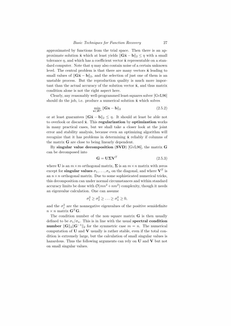
By singular value decomposition (SVD) [GvL96], the matrix G
can be decomposed into
G = UΣVT (2.5.3)
where U is an m×m orthogonal matrix, Σ is an m×n matrix with zeros
except for singular values σ1, . . . , σn on the diagonal, and where VT is
an n×n orthogonal matrix. Due to some sophisticated numerical tricks,
this decomposition can under normal circumstances and within standard
accuracy limits be done with O(mn2 +nm2) complexity, though it needs
an eigenvalue calculation. One can assume
σ21 ≥ σ2
2 ≥ . . . ≥ σ2n ≥ 0,
and the σ2j are the nonnegative eigenvalues of the positive semidefinite
n× n matrix GT G.
The condition number of the non–square matrix G is then usually
defined to be σ1/σn. This is in line with the usual spectral condition
number ‖G‖2‖G−1‖2 for the symmetric case m = n. The numerical
computation of U and V usually is rather stable, even if the total con-
dition is extremely large, but the calculation of small singular values is
hazardous. Thus the following arguments can rely on U and V but not
on small singular values.
28
Using (2.5.3), the solution of either the minimization problem (2.5.2)
or, in the case m = n, the solution of (2.5.1) can be obtained and
analyzed as follows. We first introduce new vectors
c := UT b ∈ IRm and y := VT x ∈ IRn
by transforming the data and the unknowns orthogonally. Since orthog-
onal matrices preserve Euclidean lengths, we rewrite the squared norm
as
‖Gx − b‖22 = ‖UΣVT x − b‖2
2
= ‖ΣVT x− UT b‖22
= ‖Σy − c‖22
=
n∑
j=1
(σjyj − cj)2 +
m∑
j=n+1
c2j
where now y1, . . . , yn are variables. Clearly, the minimum exists and is
given by the equations
σjyj = cj , 1 ≤ j ≤ n,
but the numerical calculation runs into problems when the σj are small
and imprecise in absolute value, because then the resulting yj will be
large and imprecise. The final transition to the solution x = Vy by an
orthogonal transformation does not improve the situation.
If we assume existence of a good solution candidate x = Vy with
‖Gx− b‖2 ≤ η, we have
n∑
j=1
(σj yj − cj)2 +
m∑
j=n+1
c2j ≤ η2. (2.5.4)
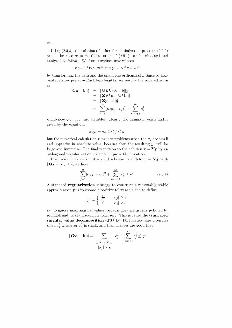
A standard regularization strategy to construct a reasonably stable
approximation y is to choose a positive tolerance ǫ and to define
yǫj :=
cj
σj|σj | ≥ ǫ
0 |σj | < ǫ
i.e. to ignore small singular values, because they are usually polluted by
roundoff and hardly discernible from zero. This is called the truncated
singular value decomposition (TSVD). Fortunately, one often has
small c2j whenever σ2j is small, and then chances are good that
‖Gxǫ − b‖22 =
∑
1 ≤ j ≤ n
|σj | ≥ ǫ
c2j +
m∑
j=n+1
c2j ≤ η2

Basic Techniques for Function Recovery 29
holds for xǫ = Vyǫ.
0 50 100 150 200 250 300 350 400 450−18
−16
−14
−12
−10
−8
−6
−4
−2
0
2
Number of DOF
Log of linear system error−log of condition of subsystem
Fig. 2.7. Error and condition of linear subsytems via SVD
Figure 2.7 is an example interpolating the MATLAB peaks function
in m = n = 441 regular points on [−3, 3]2 by Gaussians with scale 1,
using the standard system (1.2.2). Following a fixed 441× 441 singular
value decomposition, we truncated after the k largest singular values,
thus using only k degrees of freedom. The results for 1 ≤ k ≤ 441
show that there are low-rank subsystems which already provide good
approximate solutions. A similar case for the Method of Fundamental
Solutions will be provided by Example 4.5.1 in Chapter 4.
But now we proceed with our analysis. In case of large cj for small σj ,
truncation is insufficient, in particular if the dependence on the unknown
noise level η comes into focus. At least, the numerical solution should
not spoil the reproduction quality guaranteed by (2.5.4), which is much
more important than an exact calculation of the solution coefficients.
Thus one can minimize ‖y‖22 subject to the essential constraint
n∑
j=1
(σjyj − cj)2 +
m∑
j=n+1
c2j ≤ η2, (2.5.5)

30
10−25
10−20
10−15
10−10
10−5
100
10−9
10−8
10−7
10−6
10−5
10−4
10−3
10−2
10−1
100
Delta
Err
or
Error without noiseError with 0.01% noise
Fig. 2.8. Error as function of regularization parameter δ2
but we suppress details of the analysis of this optimization problem.
Another, more popular possibility is to minimize the objective function
n∑
j=1
(σjyj − cj)2 + δ2
n∑
j=1
y2j
where the positive weight δ allows placing more emphasis on small co-
efficients if δ is increased. This is called Tikhonov regularization.
The solutions of both settings coincide and take the form
yδj :=
cjσj
σ2j + δ2
, 1 ≤ j ≤ n,
depending on the positive parameter δ of the Tikhonov form, and for
xδ := Vyδ we get
‖Gxδ − b‖22 =
n∑
j=1
c2j
(δ2
δ2 + σ2j
)2
+m∑
j=n+1
c2j ,
which can me made smaller than η2 for sufficiently small δ. The optimal
value δ∗ of δ for a known noise level η in the sense of (2.5.5) would be

Basic Techniques for Function Recovery 31
0 50 100 150 200 250 300 350 400 45010
−14
10−12
10−10
10−8
10−6
10−4
10−2
100
102
j
Rat
ioc coefficients for data without noisec coefficients for data with 0.01% noise
Fig. 2.9. Coefficients |cj | as function of j
defined by the equation ‖Gxδ∗ − b‖22 = η2, but since the noise level is
only rarely known, users will be satisfied to achieve a tradeoff between
reproduction quality and stability of the solution by inspecting the error
‖Gxδ − b‖22 for varying δ experimentally.
We now repeat the example leading to Figure 2.7, replacing the trun-
cation strategy by the above regularization. Figure 2.8 shows how the
error ‖Gxδ −b‖∞,X depends on the regularization parameter δ. In case
of noise, users can experimentally determine a good value for δ even for
an unknown noise level. The condition of the full matrix was calculated
by MATLAB as 1.46 · 1019, but it may actually be higher. Figure 2.9
shows that the coefficients |cj | are indeed rather small for large j, and
thus regularization by truncated SVD will work as well in this case.
From Figures 2.9 and 2.8 one can see that the error ‖Gxδ−b‖ takes a
sharp turn at the noise level. This has led to the L–curve method for
determining the optimal value of δ, but the L-curve is defined differently
as the curve
δ 7→ (log ‖yδ‖22, log ‖Gxδ − b‖2
2).
The optimal choice of δ is made where the curve takes its turn, if it does

32
10−5
100
105
1010
1015
1020
10−18
10−16
10−14
10−12
10−10
10−8
10−6
10−4
10−2
100
L−curve for data without noiseL−curve for data with 0.01% noise
Fig. 2.10. The L-curve for the same problem
so, and there are various ways to estimate the optimal δ (see [Han92,
Han94, Han00]) including a MATLAB software package.
Figure 2.10 shows the typical L-shape of the L-curve in case of noise,
while in the case of exact data there is no visible sharp turn within
the plot range. The background problem is the same as for the previous
figures. A specific example within the Method of Fundamental Solutions
will be presented in Section 4.9 on inverse problems.
Consequently, users of radial basis function techniques are strongly
advised to take some care when choosing a linear system solver. The
solution routine should incorporate a good regularization strategy or at
least automatically project to stable subspaces and not give up quickly
due to bad condition. Further examples for this will follow in later
chapters of the book.
But for large systems the above regularization strategies are debat-
able. A singular-value decomposition of a large system is computation-
ally expensive, and the solution vector will usually not be sparse, i.e. the
evaluation of the final solution at many points is costly. In Section 2.9 we
shall demonstrate that linear systems arising from radial basis functions
often have good approximate solutions with only few nonzero coeffi-

Basic Techniques for Function Recovery 33
cients. The corresponding numerical techniques are other, and possibly
preferable regularizations which still are under investigation. A simple
but efficient recent strategy [Sch07a] is to project the right–hand side of
the system (2.5.1) to the span of adaptively selected columns of G.
2.6 Scaling
If radial basis functions are used directly, without any additional tricks
and treats, users will quickly realize that scaling is a crucial issue. The
literature has two equivalent ways of scaling a given radial basis function
φ, namely replacing it by either φ(‖x− y‖2/c) or by φ(ǫ‖x− y‖2) with
c and ǫ being positive constants. Of course, these scalings are equiva-
lent, and the case ǫ → 0, c → ∞ is called the flat limit [DF02]. In
numerical methods for solving differential equations, the scale factor c
is preferred, and it is called shape factor there. Readers should not be
irritated by slightly different ways of scaling, e.g.
φc(‖x‖2) :=√c2 + ‖x‖2
2 = c ·√
1 +‖x‖2
2
c2= c · φ1
(‖x‖2
c
)(2.6.1)
for multiquadrics, because the outer factor c is irrelevant when forming
trial spaces from functions (1.1.1). Furthermore, it should be kept in
mind that only the polyharmonic spline and its special case, the
thin–plate spline, generate trial spaces which are scale-invariant.
Like the tradeoff between error and stability when choosing smooth-
ness (see the preceding section), there often is a similar tradeoff induced
by scaling: a “wider” scale improves the error behavior but induces in-
stability. Clearly, radial basis functions in the form of sharp spikes will
lead to nearly diagonal and thus well-conditioned systems (1.2.2), but
the error behavior is disastrous, because there is no reproduction quality
between the spikes. The opposite case of extremely “flat” and locally
close to constant radial basis functions leads to nearly constant and thus
badly conditioned matrices, while many experiments show that the re-
production quality is even improving when scales are made wider, as far
as the systems stay solvable.
For analytic radial basis functions (i.e. in C∞ with an expansion into
a power series), this behavior has an explanation: the interpolants often
converge towards polynomials in spite of the degeneration of the linear
systems [DF02, Sch05, LF05, LYY05, Sch06a]. This has implications
for many examples in this book which approximate analytic solutions
of partial differential equations by analytic radial basis functions like

34
10−1
100
101
102
10−3
10−2
10−1
100
Gauss, scale=1
Wendland C2, scale=10
Thin−plate spline, scale=1
Inverse Multiquadric, scale=1
Multiquadric, scale=1
Fig. 2.11. Error as function of relative scale, smooth case
Gaussians or multiquadrics: whatever is calculated is close to a good
polynomial approximation to the solution. Users might try using poly-
nomials right away in such circumstances, but the problem is to pick a
good polynomial basis. For multivariate problems, choosing a good poly-
nomial basis must be data-dependent, and it is by no means clear how
to do that. It is one of the intriguing properties of analytic radial basis
functions that they automatically choose good data-dependent polyno-
mial bases when driven to their “flat limit”. There are new techniques
[LF03, FW04] which circumvent the instability at large scales, but these
are still under investigation.
Figure 2.11 shows the error for interpolation of the smooth MATLAB
peaks function on a fixed data set, when interpolating radial basis func-
tions φ are used with varying scale relative to a φ-specific starting scale
given in the legend. Only those cases are plotted which have both an
error smaller than 1 and a condition not exceeding 1012. Since the data
come from a function which has a good approximation by polynomials,
the analytic radial basis functions work best at their condition limit.
But since the peaks function is a superposition of Gaussians of different

Basic Techniques for Function Recovery 35
10−2
10−1
100
101
102
10−2
10−1
100
Gauss, scale=1
Wendland C2, scale=10
Thin−plate spline, scale=10
Inverse Multiquadric, scale=1
Multiquadric, scale=1
Fig. 2.12. Error as function of relative scale, nonsmooth case
scales, the Gaussian radial basis function still shows some variation in
the error as a function of scale.
Interpolating the nonsmooth function (2.3.2) shows a different behav-
ior (see Figure 2.12), because now the analytic radial basis functions
have no advantage for large scales. In both cases one can see that the
analytic radial basis functions work well only in a rather small scale
range, but there they beat the other radial basis functions. Thus it of-
ten pays off to select a good scale or to circumvent the disadvantages of
large scales [LF03, FW04].
As in finite element methods, users might want to scale the basis func-
tions in a data-dependent way, making the scale c in the sense of using
φ(‖x − y‖2/c) proportional to the fill distance h as in (2.3.1). This is
often called a stationary setting, e.g. in the context of wavelets and
quasi-interpolation. If the scale is fixed, the setting is called nonsta-
tionary, and this is what we have been considering up to this point.
Users must be aware that the error and stability analysis, as described
in the previous sections, apply to the nonstationary case, while the sta-
tionary case will not converge for h → 0 in case of unconditionally
36
10−0.6
10−0.4
10−0.2
100
100.2
10−9
10−8
10−7
10−6
10−5
10−4
10−3
10−2
10−1
100
101
Gauss, start scale=8
Wendland C2, start scale=100
Thin−plate spline, start scale=1
Inverse Multiquadric, start scale=20
Multiquadric, start scale=15
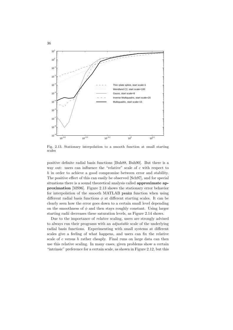
Fig. 2.13. Stationary interpolation to a smooth function at small startingscales
positive definite radial basis functions [Buh88, Buh90]. But there is a
way out: users can influence the “relative” scale of c with respect to
h in order to achieve a good compromise between error and stability.
The positive effect of this can easily be observed [Sch97], and for special
situations there is a sound theoretical analysis called approximate ap-
proximation [MS96]. Figure 2.13 shows the stationary error behavior
for interpolation of the smooth MATLAB peaks function when using
different radial basis functions φ at different starting scales. It can be
clearly seen how the error goes down to a certain small level depending
on the smoothness of φ and then stays roughly constant. Using larger
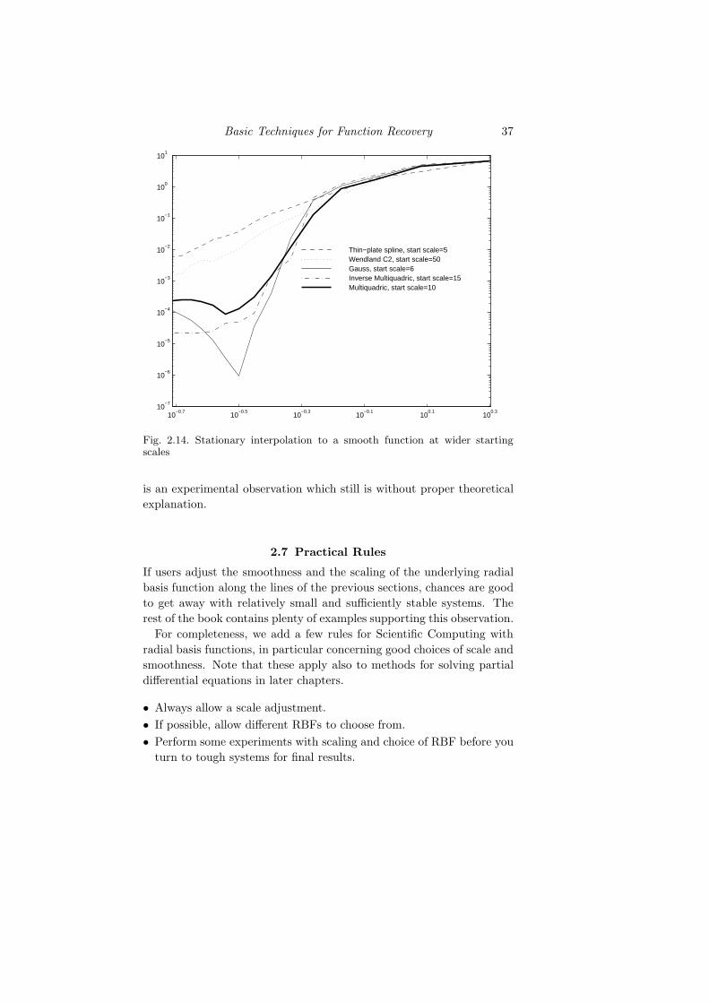
starting radii decreases these saturation levels, as Figure 2.14 shows.
Due to the importance of relative scaling, users are strongly advised
to always run their programs with an adjustable scale of the underlying
radial basis functions. Experimenting with small systems at different
scales give a feeling of what happens, and users can fix the relative
scale of c versus h rather cheaply. Final runs on large data can then
use this relative scaling. In many cases, given problems show a certain
“intrinsic” preference for a certain scale, as shown in Figure 2.12, but this
Basic Techniques for Function Recovery 37
10−0.7
10−0.5
10−0.3
10−0.1
100.1
100.3
10−7
10−6
10−5
10−4
10−3
10−2
10−1
100
101
Gauss, start scale=6Wendland C2, start scale=50Thin−plate spline, start scale=5
Inverse Multiquadric, start scale=15Multiquadric, start scale=10
Fig. 2.14. Stationary interpolation to a smooth function at wider startingscales
is an experimental observation which still is without proper theoretical
explanation.
2.7 Practical Rules
If users adjust the smoothness and the scaling of the underlying radial
basis function along the lines of the previous sections, chances are good
to get away with relatively small and sufficiently stable systems. The
rest of the book contains plenty of examples supporting this observation.
For completeness, we add a few rules for Scientific Computing with
radial basis functions, in particular concerning good choices of scale and
smoothness. Note that these apply also to methods for solving partial
differential equations in later chapters.
• Always allow a scale adjustment.
• If possible, allow different RBFs to choose from.
• Perform some experiments with scaling and choice of RBF before you
turn to tough systems for final results.
38
• If you do not apply iterative solvers, do not worry about large con-
dition numbers, but use a stabilized solver, e.g. based on Singular
Value Decomposition (SVD). Remember that unless you apply cer-
tain tricks, getting a good reproduction quality will always require
bad condition. If you need k decimal digits of final accuracy for an
application, do not bother about condition up to 1012−k.
• If you use compactly supported radial basis functions, do not expect
them to work well when each support contains less than about 50
neighbors. This means that the bandwidth of large sparse systems
should not be below 50. Increasing bandwidth will usually improve
the quality of the results at the expense of computational complexity.
• When using either compactly supported or quickly decaying radial
basis functions of high smoothness, the theoretical support and the
practical support do not coincide. In such cases one should enforce
sparsity by chopping the radial basis functions, in spite of losing pos-
itive definiteness properties. But this should be done with care, and
obeying the “50 neighbors” rule above.
• If systems get large and ill–conditioned, and if change of scale and
RBF do not improve the situation, try methods described in the fol-
lowing section.
• Use blockwise iteration (“domain decomposition”) first, because it is
simple and often rather efficient.
• Blockwise iteration can be speeded up by precalculation of LR de-
compositions of blocks.
• If all of this does not work, try partitions of unity, multilevel methods,
or special preconditioning techniques. You are now at current research
level, and you should look into the next section.
2.8 Large Systems: Computational Complexity
Handling unavoidably large problems raises questions of computational
complexity which deserve a closer look. First, there is the difference be-
tween the complexities of solving and evaluation. The latter addresses
the evaluation of trial functions like (1.2.5) for large n at many evalu-
ation points x ∈ IRd, while the former concerns the calculation of the
coefficients.
Evaluation complexity can be kept at bay by localization techniques
needing only a few “local” coefficients to evaluate the trial function.
There are several possibilities for localization:

Basic Techniques for Function Recovery 39
• Using compactly supported radial basis functions [Wu95, Wen95,
Buh98] leads to sparse systems and localized evaluation. In particu-
lar, Wendland’s functions have been applied successfully in plenty of
applications, e.g. [FI96, CBP99, SW99, CBP99, CMC99, WHL+99,
CYT00a, CYT00b, GCG00, MYP+01, CGGC02, WHG02a, WHG02b,
KSBH02, OBS03, Fas03, RTSD03, WK05, ABW06] and many others.
Since the correspondent radial basis functions have limited smooth-
ness (and thus low convergence rates, following section 2.3), the er-
ror will be larger than when using analytic radial basis functions,
but the stability is much better. However, they again need care-
ful scaling, which now influences the evaluation complexity and the
sparsity. “Flat” scaling improves the error behavior at the price of
increasing instability and complexity. Together with thinning algo-
rithms providing data at different resolution levels, compactly sup-
ported radial basis functions also allow efficient multiscale tech-
niques [FI96, Fas98, Fas99, NSW99, GFJ00, CGGC02, Isk04].
• partition of unity methods [MB96, BM97, GS00, GS02a, GS02b,
Wen02, Sch03, OBS03, TRS04] are a flexible and general tool for lo-
calizing any trial space. They have the advantage of not spoiling the
local error behavior of the original trial space while localizing both
the evaluation and the solving. The basic idea is to start with a se-
lection of smooth “weight” functions ϕi : IRd → IR with overlapping
compact supports Ωi and summing up to 1 globally. If a trial space
Ui is given on each of the subdomains Ωi, a global trial function u can
be superimposed from local trial functions ui ∈ Ui by the localized
summation
u(x) :=∑
i
ui(x)ϕi(x) =∑
i : x∈Ωi
ui(x)ϕi(x).
Depending on the problem to be solved, one can plug the above rep-
resentation into the full problem or use local methods to generate
the local trial functions ui more or less independently, thus localizing
also the solution stage. This class of techniques deserves much more
attention from scientists and engineers working in applications.
• multipole expansions work best for radial basis functions with se-
ries expansions around infinity. They aggregate “far” points into “pan-
els” and use expansions to simplify evaluation. This technique is very
successful in certain applications [BN92, BG97, BL97, BC00, BCR00,
CBN02] though it is not easy to code.

40
• Fast evaluation using transforms is another choice [PS03, FS04,
RB05], but it has not yet found its way into applications.
The dominant methods for reducing the complexity of solving large sys-
tems like (1.2.2) are domain decomposition and preconditioning.
In classical analysis, domain decomposition means the splitting of a
boundary value problem into smaller boundary value problems, using in-
terface conditions for coupling the local problems. This was also done for
problems solved via radial basis functions (e.g. [ZHL03a, LH04, ICT04]),
but the majority of authors working with radial basis functions use the
term in a different way. We explain it below, together with its close
connection to preconditioning.
Of course, one can solve a huge problem (1.2.2) or (1.2.7) by a block–
wise Gauss-Seidel or Jacobi iteration, where each “block” is defined by
taking a small set of points in a small subdomain. Each block defines a
local linear system where the unused data are shifted to the right-hand
side [WHL+99]. These local systems are solved independently and in
turn. It does not matter whether the domains overlap or not. In most
cases the numerical results for suitably chosen subdomains usually are
much better than for direct iterative methods. In particular, the LU
decompositions of the small local systems can be stored and re-used all
over again in order to save computation time. Furthermore, there are
different strategies for choosing “good” blocks.
This basic technique comes in various forms. It can be reformulated
as a block–wise preconditioner or as a Krylov subspace iteration
[FP00, FGP05] employing local cardinal functions in case of plain
interpolation [BCM99, BLB00, KH00, Mou01, LK04, LK05, BLKL05].
It can also be seen as an additive [HW00] or as a multiplicative Schwarz
decomposition [BLB00] depending whether Jacobi or Gauss-Seidel is
used as the inner iteration. For regular data these preconditioners can
achieve a fixed accuracy by a fixed number of iterations of the conjugate
gradient method which is not dependent on the number of equations
[Bax02].
Altogether, there are many successful techniques for handling large
and ill–conditioned systems (see e.g. an overview in [KH00]), and there
are a few promising theoretical investigations [BCM99, FP00, Bax02,
BLKL05, FGP05, Sch05], but a general and complete mathematical
foundation for handling large RBF–based systems arising in Partial Dif-
ferential Equations still is missing.

Basic Techniques for Function Recovery 41
2.9 Sensitivity to Noise
So far the discussion has focused on noiseless data, with the exception of
Figure 2.8. If users expect noise in the data, an interpolatory recovery
along the lines of Section 2.1 is not appropriate, because it treats noise as
data. In most of the later sections of this book, data are right-hand sides
or boundary values for partial differential equations, and they usually
are given as noiseless functions which can be evaluated anywhere. Thus
the rest of the book does not treat noisy inputs in detail. But at this
point some remarks are appropriate.
In all noisy situations, interpolation should be replaced by approxi-
mation. This can be done in various ways leading to stabilization.
A primitive, but often quite sufficient technique is to run a smoothing
process on the raw data and to recover the unknown function from the
smoothed data instead of the raw data.
Another standard trick is to solve (1.2.2) in the L2 sense with over-
sampling, if only n << m trial centers xj are used for m data points yk.
The trial centers can then be placed rather freely with a large separation
distance, while a small separation distance of data points will not have a
dramatic effect on stability any more. However, there is not very much
theoretical and practical work done on unsymmetric recovery techniques
[Sch07b, Sch06c, Sch06a].
A third possibility is the old Levenberg–Marquardt trick of adding
a positive value λ into the diagonal of the kernel matrix of (1.2.2)
with entries φ(‖xj − xk‖2). As is well-known from literature on spline
smoothing, this leads to an approximant achieving a tradeoff between
smoothness and reproduction quality which can be controlled by λ. If
a stochastic background is available, there are methods to estimate λ
properly, e.g. by cross–validation. However, in most cases users adjust
λ experimentally. This technique also helps to fight instability when
working on irregularly distributed data [WR05], because it is able to shift
the stability from dependence on the separation distance to dependence
on the fill distance (see Section 2.4).
A fourth possibilty is regularization, for example, using a singular-
value decomposition as described in Section 2.5.
In general, one can replace the system (1.2.2) by an optimization
method which penalizes the reproduction error on the one hand and
either a complexity or smoothness criterion on the other, allowing a fair
amount of control over the tradeoff between error and stability. Penalties
for the discrete reproduction error can be made in various discrete norms,

42
the ℓ1 and ℓ∞ case having the advantage of leading to linear optimization
restrictions, while the discrete ℓ2 norm leads to quadratic ones. For
radial basis functions of the form (1.1.1) or (1.2.5), the quadratic form
‖u‖2φ :=
n∑
j,k=1
αjαkφ(‖xj − xk‖2) (2.9.1)
is a natural candidate for penalizing high derivatives without evaluating
any. This is due to the standard fact that the above expression is a
squared norm in a native Hilbert space of functions with about half
the smoothness of φ, penalizing all available derivatives there. For de-
tails, we have to refer to basic literature [Buh03, Wen05] on the theory
of radial basis functions. But even though we skip over native spaces
here, all users should be aware that they always lurk in the theoreti-
cal background, and that all methods based on radial basis functions
implicitly minimize the above quadratic form under all functions in the
native space having the same data. This has a strong regularization ef-
fect which is the background reason why radial basis functions or more
general kernel methods work well for many ill-posed and inverse
problems [HW03, Li04, TWN04, CC05b, CC05a, HW05, JZ05, Li05,
Sai05, Nas06]. The above strategy of minimizing the quadratic form
(2.9.1) also is central for modern methods of machine learning, but
we cannot pursue this subject in detail here [CST00, SS02, STC04].
Let us use minimization of the quadratic form (2.9.1) to provide an
example of the tradeoff between error and complexity. Again, the basic
situation is interpolation to the MATLAB peaks function, this time in
14×14=196 regularly distributed points in [−3, 3]2 by Gaussians of scale
1. The global L∞[−3, 3]2 error of the exact interpolation on these data
is 0.024, evaluated on a fine grid with 121×121=14641 points. But now
we minimize the quadratic form (2.9.1) under the constraints
−ǫ ≤n∑
j=1
αjφ(‖xj − xk‖2) − f(xk) ≤ ǫ, 1 ≤ k ≤ n (2.9.2)
for positive ǫ. The case of ǫ = 0 is exact interpolation using all 196 data
points and trial functions. For positive ǫ, the usual Karush-Kuhn-Tucker
conditions imply that only those points xk are actually used where one
of the bounds in (2.9.2) is attained with equality. The number n(ǫ) of
required points increases to the maximally possible n(0) = 196 when ǫ
decreases. Figure 2.15 shows this for the case of exact and noisy data.
But even more interesting is the behavior of the global L∞[−3, 3]2

Basic Techniques for Function Recovery 43
0 20 40 60 80 100 120 140 160 180 2000
0.1
0.2
0.3
0.4
0.5
0.6
0.7
0.8
0.9
1
Points
Eps
ilon
no noise2 % noise
Fig. 2.15. Connection between ǫ and the number n(ǫ) of necessary points
error E(ǫ) as a function of ǫ. Figure 2.16 shows that E(ǫ) roughly follows
the behavior of ǫ when plotted as a function of the required points n(ǫ).
Both curves are experimentally available, and one can read off that the
optimal choice of ǫ in the noisy case is at the point where the curve takes
its L-turn, i.e. at the point of largest curvature around n = 40. This
can be viewed as an experimental method to determine the noise level.
Note that it does not pay off to use more points, and note the similarity
to the L-curve technique [HO93].
But these curves are also useful for exact data,. Since the maximum
value of the peaks function is about 8.17, one can get a relative global
accuracy of 1% using roughly 60 points for exact data. It makes no
sense to use the full 196 points, even for exact data, if exact results are
not required. Of course, larger noise levels lead to smaller numbers of
required points, but a thorough investigation of these tradeoff effects
between error and complexity is still a challenging research topic.
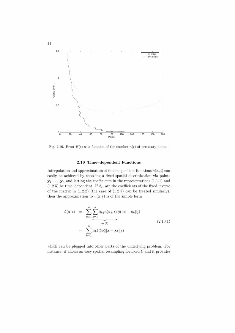
44
0 20 40 60 80 100 120 140 160 180 2000
0.5
1
1.5
Points
Glo
bal e
rror
no noise2 % noise
Fig. 2.16. Error E(ǫ) as a function of the number n(ǫ) of necessary points
2.10 Time–dependent Functions
Interpolation and approximation of time–dependent functions u(x, t) can
easily be achieved by choosing a fixed spatial discretization via points
y1, . . . ,yn and letting the coefficients in the representations (1.1.1) and
(1.2.5) be time–dependent. If βij are the coefficients of the fixed inverse
of the matrix in (1.2.2) (the case of (1.2.7) can be treated similarly),
then the approximation to u(x, t) is of the simple form
u(x, t) =
n∑
k=1
n∑
j=1
βkju(xj , t)
︸ ︷︷ ︸αk(t)
φ(‖x − xk‖2)
=
n∑
k=1
αk(t)φ(‖x − xk‖2)
(2.10.1)
which can be plugged into other parts of the underlying problem. For
instance, it allows an easy spatial resampling for fixed t, and it provides

Basic Techniques for Function Recovery 45
arbitrary approximate derivatives such as
∂u
∂xj=
n∑
k=1
αk(t)∂φ(‖x − xk‖2)
∂xj=
n∑
k=1
n∑
j=1
βkju(xj , t)∂φ(‖x − xk‖2)
∂xj
in terms of time–dependent values of either u or the coefficients αk.
Formulas like this are useful when considering time-dependent meshless
spatial discretizations, because they make resampling easy, avoiding re-
meshing.
But the above technique can also serve for line methods solving
partial differential equations like
∂u
∂t(x, t) = F (L(u(x, t)),x, t) (2.10.2)
with a linear spatial differential operator L because of
α′k(t) =
n∑
j=1
βkj∂u
∂t(xj , t), 1 ≤ k ≤ n
=
n∑
j=1
βkjF
(n∑
k=1
αk(t)L(φ(‖x − xk‖2))|x=xj,xj , t
).
leading to a system of ordinary differential equations. Along these lines.
radial basis function methods will be used in later parts of the book, in
particular in chapters 3 and 6.

3
Collocation Techniques
The history of Scientific Computing shows that important numerical
techniques like
• finite difference methods,
• finite element methods,
• finite volume methods,
• boundary element methods,
• particle methods, and
• multipole methods
were introduced and improved by engineers or physicists working in ap-
plications. Similarly, the use of radial basis functions for scattered data
interpolation, as described in Chapter 2, was first introduced in 1951 by
the South African geophysicist D.G. Krige [Kri51] within a statistical
background, and called Kriging afterwards. It was further developed
by G. Matheron [Mat62] and used without any statistical background
by the geophysicist R. Hardy [Har71] who introduced multiquadrics.
Also, the use of radial basis functions for solving partial differential
equations was started not by a mathematician, but rather by the physi-
cist E. Kansa [Kan86] who proposed the meshless collocation method
for solving partial differential equations using multiquadrics, as sketched
in Section 1.6. Since the resulting system (1.6.3) of linear equations is
asymmetric, the method is now known as the asymmetric collocation
method.
Subsequently, meshless methods based on radial basis functions
have reached more and more application areas, because they provide
efficient and easy-to-use numerical techniques for solving various kinds
of partial differential equations. In the following sections, the advantages
of the asymmetric meshless collocation method are demonstrated by
46

Collocation Techniques 47
solving some typical partial differential equation problems. Since it is
impossible to give a comprehensive survey over all relevant applications,
we confine ourselves to a few special cases. These include time-dependent
problems where we use asymmetric collocation in the spatial variables
only, letting the coefficients of the spatial representation (1.1.1) be time-
dependent as in (2.10.1) of Section 2.10. Readers will notice that the
general rules governing error, stability, and scaling will be the same as
in the previous chapter.
For other time-dependent problems, the combination of the asymmet-
ric meshless collocation method with Laplace transform techniques
was successfully demonstrated in [ME94] to greatly reduce the spatial
and temporal truncation errors, and we shall deal with this special ap-
proach in Chapter 6 because it is closely related to the Helmholtz equa-
tion arising in Chapters 4 and 5.
3.1 High Dimensional Problems
Due to the restrictive requirements of grid generation when using fi-
nite difference methods or mesh generation in finite elements, the ex-
tendability of these mesh-dependent numerical methods to solve high-
dimensional problems or problems with complicated boundaries has been
prohibitive. To illustrate the adaptability of the asymmetric meshless
collocation method described in Section 1.6 for problems in higher di-
mensions, we consider the following
Example 3.1.1
∆u = fΩ in Ω := [0, 1]d
u = fΓ in Γ := ∂Ω,(3.1.2)
where d is the dimension of the space. This is of the form (1.6.1) with
the Laplace operator L := ∆.
The exact solution of (3.1.2) is given by
u(x) =
d∏
i=1
sin(xi), x = (x1, x2, . . . , xd)T
from which the values fΩ and fΓ can then be determined.
For numerical comparison we use both the asymmetric and symmet-
ric collocation methods described in Section 1.6 to solve the bound-
ary value problem (3.1.2), respectively. In the computations, the radial

48
basis function φ(r) is chosen to be r5 to avoid scaling problems. To
keep the maximum total number of points used in the computations less
than 750, we chose the trial centers and the test points to be the same
xi, i = 1 . . .m := mΩ + mΓ which are uniformly distributed in the do-
main Ω ∪ Γ so that m = sd where s = 5, . . . , 21 for d = 2, s = 5, . . . , 9
when d = 3, s = 4 and 5 when d = 4. The maximal degree of the
additional polynomials is 2.
By assuming that the solution u of (3.1.2) can be approximated by
u(x) :=
m∑
i=1
αiφ(‖x − xi‖2) +
q∑
ℓ=1
βℓpℓ(x),
where φ(r) := r5, it follows from Section 1.6 that the system of linear
equations for asymmetric collocation is a special case of (1.6.3) in the
form
m∑
k=1
αk∆φ(‖xΩj − xk‖2) +
q∑
ℓ=1
βℓ∆pℓ(xΩj ) = fΩ(xΩ
j ), j ≤ mΩ
m∑
k=1
αkφ(‖xΓj − xk‖2) +
q∑
ℓ=1
βℓpℓ(xΓj ) = fΓ(xΓ
j ), j ≤ mΓ
n∑
k=1
αkpℓ(xk) + 0 = 0, ℓ ≤ q.
For symmetric collocation, the system of linear equations is similarly
obtained from Section 1.6 as (1.6.5). Both resultant systems of equations
for the undetermined coefficients are solved by Gaussian elimination.
The results of computations for dimensions 2, 3, and 4 are listed in
Tables 3.1 and 3.2. 2
Two features can be read from these tables:
(i) For each fixed space dimension, the accuracy of the numerical
solution improves with the total number of trial centers.
(ii) If rows with m = sd points are compared for fixed s, leading
to a dimension-independent fill distance of h = 1/2s in the L∞norm, the convergence rates of both asymmetric and symmetric
collocation increase with the space dimension.
The first feature must be expected from results on interpolation and
approximation, as summarized in Section 2.3, but the second observa-
tion is surprising. It is well known from certain stationary interpolation
processes on regular data [Buh03], but its mathematical foundation must

Collocation Techniques 49
Table 3.1. Asymmetric collocation with φ(r) = r5
Dimension Points Max Error Average Error Condition Number
2 52 2.605E-3 1.391E-3 2.673E+52 102 2.179E-4 1.345E-4 1.580E+82 152 5.774E-5 3.292E-5 3.926E+92 202 2.036E-5 1.200E-5 3.445E+10
3 53 2.521E-3 1.255E-3 9.420E+63 73 5.973E-4 3.756E-4 2.083E+83 93 2.126E-4 1.440E-4 1.964E+9
4 44 7.475E-3 2.788E-3 4.555E+74 54 1.041E-3 8.518E-4 6.313E+8
2 52 2.605E-3 1.391E-3 2.673E+53 53 2.521E-3 1.255E-3 9.420E+64 54 1.041E-3 8.518E-4 6.313E+8
Table 3.2. Symmetric collocation with φ(r) = r5
Dimension Points Max Error Average Error Condition Number
2 52 4.429E-3 3.138E-3 2.897E+62 102 4.667E-4 3.307E-4 1.924E+92 152 1.246E-4 8.440E-5 5.190E+102 202 5.011E-5 3.196E-5 4.888E+11
3 53 4.749E-3 2.054E-3 1.188E+83 73 2.811E-3 1.073E-3 5.054E+93 93 1.448E-3 5.895E-4 6.120E+10
4 44 6.489E-3 2.807E-3 1.370E+84 54 3.343E-3 1.668E-3 4.673E+9
2 52 4.429E-3 3.138E-3 2.897E+63 53 4.749E-3 2.054E-3 1.188E+84 54 3.343E-3 1.668E-3 4.673E+9
be omitted here. For solving partial differential equations, the observed
increase of the convergence rate with the space dimension has no theo-
retical basis yet.

50
3.2 Transport Problems
The advantage of using radial basis functions within collocation methods
will further be illustrated by solving the nonlinear Burgers equation
ut + uux = νuxx, ν > 0. (3.2.1)
It is an extremely simplified limit form of the Navier-Stokes equation,
and it models flows of viscous liquids as well as of cars in traffic. This
equation has been studied by many researchers for the following reasons:
(i) It contains the simplest form of a nonlinear advection term uux
and a dissipation term νuxx for simulating the physical phenom-
ena of wave motion,
(ii) its analytical solution was obtained by Cole [Col51], so that errors
of numerical computations can be evaluated, and
(iii) its solutions show a shock wave behavior [Bur40] when the Rey-
nolds number 1/ν is large, i.e. when ν is small.
Various techniques have been applied to solve equation (3.2.1) numeri-
cally under the boundary conditions
u(0, t) = 0 = u(1, t), t > 0, (3.2.2)
and the initial condition
u(x, 0) = f(x), x ∈ Ω = (0, 1). (3.2.3)
We first discretize the equation (3.2.1) by using a forward difference
approximation for the time derivative to obtain
uk + δt(uk−1uk
x − νukxx) = uk−1, k ≥ 1, (3.2.4)
where δt is the length of the time step and uk denotes the kth iterate of
the solution. We approximate uk at each iteration k by multiquadrics
uk(x) ≃m∑
j=0
αkj
√(x− xj)2 + c2j + αk
m+1x+ αkm+2, (3.2.5)
where xj are (m + 1) distinct uniformly distributed centers in [0, 1].
The scale factor cj is one of the key factors for obtaining an accurate
solution, but we do not elaborate on its choice here. We just note that
an exponential variation in the scaling factors was proposed in [Kan90b],
and the ill–conditioning problem was further studied experimentally in
[KH00].

Collocation Techniques 51
For each iteration k we have to determine the m + 3 coefficients αkj
for 0 ≤ j ≤ m + 2. The boundary conditions (3.2.2) already give the
two equations
uk(x0) = 0 = uk(xm). (3.2.6)
We then collocate uk at m+1 distinct uniformly distributed collocation
points xj in (0, 1) using equation (3.2.4) to obtain
uk(xj) + δt
(uk−1(xj)
d
dxuk(xj) − ν
d2
dx2uk(xj)
)= uk−1(xj), k ≥ 1,
(3.2.7)
for j = 1, 2, . . . ,m+1, where u0(xj) is taken to be f(xj) from the initial
condition (3.2.3). The system of equations (3.2.6) and (3.2.7) can then
be solved by using Gaussian elimination with partial pivoting to obtain
the coefficients αkj . Note that the test points xj in (3.2.5) are different
from the trial centers xj in (3.2.7).
The analytical solution given in [Col51] for the Burgers equation
(3.2.1) subject to the boundary conditions (3.2.2) and the initial condi-
tion (3.2.3) is
u(x, t) =
2πν
∞∑
k=1
kAk sin(kπx) exp(−k2νπ2t)
A0 +∞∑
k=1
Ak cos(kπx) exp(−k2νπ2t)
,
where
Ak = 2
∫ 1
0
cos(kπx) exp
(− 1
2ν
∫ x
0
f(y)dy
)dx, k ≥ 1,
and
A0 =
∫ 1
0
exp
(− 1
2ν
∫ x
0
f(y)dy
)dx.
In the case when f(x) = sin(πx), the analytical solution derived in
[CS82] is
u(x, t) =
4πν
∞∑
k=1
kIk(1/2πν) sin(kπx) exp(−k2νπ2t)
I0(1/2πν) + 2
∞∑
k=1
Ik(1/2πν) cos(kπx) exp(−k2νπ2t)
, (3.2.8)
where Ik denotes the modified Bessel function of first kind and order
k. The difficulty in evaluating an accurate solution u(x, t) based on the

52
analytical formula (3.2.8) is due to the exponentially increasing term
Ik(1/2πν) in the series when ν is small. Using double precision floating-
point numbers with a total word length of 64 bits, we can compute u(x, t)
to four decimal digits by evaluating the two series in formula (3.2.8) for
ν down to 0.01 approximately. Unless an asymptotic formula is used, it
is not possible to compute u(x, t) using formula (3.2.8) for smaller ν. In
fact, the magnitude of Ik(1/2πν) already exceeds the limits of a 64 bit
computation when ν ≤ 1/4500. For comparison purposes, in the case
when ν = 0.0001, we adopt the accurate solution computed in [CM78]
using the Galerkin method with fully upwinded cubic functions and a
particularly small value of the spatial fill distance h.
0 0.1 0.2 0.3 0.4 0.5 0.6 0.7 0.8 0.9 10
0.1
0.2
0.3
0.4
0.5
0.6
0.7
0.8
0.9
1t=0.000
t=0.004
t=0.080
t=0.012
t=0.016
t=0.020
u
x
Fig. 3.1. Solution of the Burgers equation for ν = 10
We solve the Burgers equation (3.2.1) subject to the boundary condi-
tions (3.2.2) and the initial condition f(x) = sin(πx) using m = 10 for
different values of ν:
Case ν = 10 Here, the dissipation term dominates the advection term.
In fact, the curve of the solution u drops dramatically from the
initial data to zero within the first 0.05 seconds.
Case ν = 0.1 Now both the dissipation term and the advection term
have a balanced influence on the solution.
Case ν = 0.01 This is a first case when the advection term dominates
the dissipation term. The behavior of the solution u is very
different from the previous case as soon as advection dominates.
The solution u is a shock wave moving to the right with speed

Collocation Techniques 53
0 0.1 0.2 0.3 0.4 0.5 0.6 0.7 0.8 0.9 10
0.1
0.2
0.3
0.4
0.5
0.6
0.7
0.8
0.9
1t=0.00
t=0.20
t=0.40
t=0.60
t=0.80
t=1.00
u
x
Fig. 3.2. Solution of the Burgers equation for ν = 0.1
0 0.1 0.2 0.3 0.4 0.5 0.6 0.7 0.8 0.9 10
0.1
0.2
0.3
0.4
0.5
0.6
0.7
0.8
0.9
1u
x
t=0.0
0
t=0.2
0
t=0.4
0
t=0.60
t=0.80
t=1.00
Fig. 3.3. Solution of the Burgers equation for ν = 0.01
proportional to the magnitude of u. The numerical value of the
analytical solution is still available for comparison.
Case ν = 0.0001 Here, the advection term strongly dominates the dis-
sipation term. The peak of the shock wave remains high and
moves to the right during the first 0.5 seconds. The numerical
value of the analytical solution cannot be computed accurately
by standard methods.

54
0 0.1 0.2 0.3 0.4 0.5 0.6 0.7 0.8 0.9 10
0.1
0.2
0.3
0.4
0.5
0.6
0.7
0.8
0.9
1u
x
t=0.0
0
t=0.2
0
t=0.4
0
t=0.60
t=0.80
t=1.00
Fig. 3.4. Solution of the Burgers equation for ν = 0.0001
In Figure 3.1 to Figure 3.4, we display the profiles of the numerical
solutions uk using the global formula (3.2.5) for all cases. Similar re-
sults can also be found in [OP86] for comparison. For ν = 0.0001, we
compare the numerical results with the values obtained using the Com-
pact Difference Technique [MG80], the Finite Element Method
with a special splitting technique [IM92], and with moving nodes [CS82].
The meshless spatial collocation method offers better results than the
finite element method with moving nodes and much better results than
both the compact difference technique and finite elements with split-
ting. Results are shown in Table 3.3. With a fixed number of spatial
points, the ℓ∞-norm errors of the numerical scheme are approximately
10−2, 10−3, and 10−4 for time steps δt = 0.001, 0.0001, and 0.00001,
respectively. Altogether, this truly meshless method not only is easy to
implement, but also offers an excellent approximation for large values of
the Reynolds number. Finally, we refer the reader to [IK04] for a rather
sophisticated adaptive meshless treatment of 2D advection using radial
basis functions.
3.3 Free Boundary Value Problems
As another illustration of the advantages of meshless collocation, we
now treat the Black–Scholes equation for both European and Amer-
ican option valuation. In particular, the American option valuation can
be treated as a free boundary diffusion problem in which no analytic

Collocation Techniques 55
Compact FEM FEM Meshlessaccurate difference splitting moving (m = 10 points)
x solution δt=0.001 δt=0.1* δt=0.001* δt=0.1 δt=0.001
0.00 0.000 0.000 0.000 0.000 0.000 0.0000.05 0.042 0.050 0.041 0.042 0.042 0.0420.11 0.084 0.075 0.083 0.084 0.084 0.0840.16 0.126 0.147 0.125 0.126 0.126 0.1260.22 0.168 0.135 0.169 0.168 0.168 0.1680.27 0.210 0.261 0.203 0.210 0.210 0.2100.33 0.252 0.209 0.266 0.252 0.251 0.2520.38 0.293 0.334 0.252 0.294 0.293 0.2930.44 0.335 0.304 0.396 0.336 0.334 0.3350.50 0.376 0.417 0.235 0.377 0.375 0.3760.55 0.418 0.374 0.548 0.419 0.415 0.4180.61 0.459 0.505 0.257 0.460 0.455 0.4590.66 0.500 0.463 0.604 0.500 0.495 0.4990.72 0.540 0.580 0.601 0.541 0.534 0.5400.77 0.580 0.536 0.463 0.581 0.572 0.5800.83 0.620 0.667 0.701 0.621 0.609 0.6200.88 0.659 0.620 0.671 0.660 0.645 0.6600.94 0.698 0.741 0.726 0.699 0.678 0.6951.00 0.000 0.000 0.000 0.000 0.000 0.000
* with 16 intervals
Table 3.3. Comparison of results for ν = 0.0001.
solution is available. The difference between the two only lies in the
boundary conditions, and this is why we start with the Black–Scholes
equation and postpone the boundary conditions.
As outlined in Section 2.10 concerning line methods for time-dependent
problems, we discretize the spatial part of the computational domain
by superpositions (1.1.1) of translates of a positive definite radial ba-
sis function φ and then let the coefficients be functions of time as in
(2.10.1). Since the radial basis function can be chosen to be arbitrar-
ily continuously differentiable, higher order partial derivatives of the
trial functions can directly be computed via derivatives of the radial
basis function. This is particularly useful in computing special finan-
cial derivative terms like Delta values. To handle the time derivative
variable, the Black–Scholes equation is transformed as in (2.10.2) to a
system of first order differential equations in time whose solution can be
obtained by using an ad-hoc time integration scheme.

56
To be more explicit, consider the Black–Scholes equation
∂V
∂t+
1
2σ2S2 ∂
2V
∂S2+ rS
∂V
∂S− rV = 0, 0 < t < T, S > 0, (3.3.1)
with the terminal condition
V (S, T ) = max(E − S, 0) (3.3.2)
for European put options, where r is the risk-free interest rate, σ is the
volatility of the stock price S, and V (S, t) is the option value at time t
and stock price S. The transformations
S = Eex, t = T − τ
σ2/2, V = Eeαx+βτu(x, τ)
given in [WDH95] change equations (3.3.1) and (3.3.2) to the simple
diffusion equation
∂u
∂τ=∂2u
∂x2, −∞ < x <∞, 0 < τ <
1
2σ2T, (3.3.3)
with initial condition
u(x, 0) = max(e12 (γ−1)x − e
12 (γ+1)x, 0), (3.3.4)
where γ = rσ2/2, α = −(γ − 1)/2, and β = α2 + (γ − 1)α− γ.
Using meshless collocation in the spatial variable, an approximation
of the solution of (3.3.3) subject to the initial condition (3.3.4) is sought
as in (2.10.1) by
u(x, τ) =m∑
k=1
αk(τ)φ(x − xk), (3.3.5)
where (x, τ) ∈ [a, b] × [0, σ2T/2], and X := x1 . . . , xm is a set of m
distinct points in the interval [a, b]. Define
ΦTX(x) := (φ(x − x1), . . . , φ(x− xm)) ∈ IRm
aT (t) := (α1(t), . . . , αm(t)) ∈ IRm.
The trial space is then spanned by all functions of the form ΦTX(x)a(τ).
It is well known from the theory of radial basis function approxima-
tions that smooth functions on Ω× [0, σ2T/2] can be well approximated
by functions ΦT (x)a(τ) if the scattered points from X := x1, . . . , xmhave a sufficiently small fill distance (2.3.1) in the spatial domain Ω ⊂IRd. This was outlined in Section 2.3 and has a long history dating back
to e.g. [MN88, WS93] and summarized in [Buh03, Wen05]. To handle

Collocation Techniques 57
time derivatives, an approximation of the solution in the trial space is
constructed which satisfies (3.3.3) on the lines x = xj .
Assume that a function u of the form (3.3.5) satisfies equation (3.3.3)
on the lines x = xj . Then the vector function
u(τ)T := (u(x1, τ), . . . , u(xm, τ)) ∈ IRm
has the form u(τ) = AXa(τ) with the time-independent positive definite
kernel matrix
AX := (φ(‖xj − xk‖2))1≤j,k≤m
arising already in (1.2.2).
Substituting the representation u(τ) = AXa(τ) into equation (3.3.3),
we obtain the following system
AXa′(τ) = −AX,2a(τ)
of ordinary differential equations (ODEs) for the unknown vector func-
tion a(τ), where AX,2 is defined to be the matrix with entries consisting
of spatial derivatives −φ′′(xj − xk) for 1 ≤ j, k ≤ m.
Since AX is positive definite, its inverse A−1X exists and we have
a′(τ) = −A−1X AX,2a(τ) (3.3.6)
or equivalently
u′(τ) = −AX,2A−1X u(τ). (3.3.7)
Since φ(x) is a positive definite function, the function −φ′′(x) is a pos-
itive definite function (this follows from univariate Fourier transform
arguments we omit here), and hence AX,2 is also a positive definite
matrix.
These linear ODE systems (3.3.6) or (3.3.7) can then be solved by
using various methods. With the initial condition u(0) obtained from
the initial condition (3.3.4), the systems (3.3.6) or (3.3.7) are standard
linear initial value problems from any textbook in ordinary differential
equations, and they have explicitly available exponentially decaying so-
lutions due to the negative definiteness of the system matrix −AX,2A−1X .
Using the matrix exponential
etBx :=
∞∑
n=0
tn
n!Bnx

58
for square m × m matrices B, scalars t and vectors x ∈ IRm, our ap-
proximate solution is
u(τ) = e−τAX,2A−1X u(0). (3.3.8)
So far, the above results hold for positive definite radial basis functions,
but they can be extended to conditionally positive definite functions.
For instance, if we use scaled multiquadrics φ(x) =√c2 + x2, an ap-
proximation order O(hρ) for any ρ > 0 can be achieved if the time steps
are small enough. Note that the time stepping cannot be avoided since
the numerical computation of the eigenvalues and eigenvectors from the
explicit formula can be difficult.
We can treat the case of American options similarly. Their pricing
can be treated as a free boundary value problem, but until recently no
analytical formula was available. American options allow early exercise
at any time t ∈ [0, T ] with an optimal exercise stock value of S =
B(t). The difficulty for most numerical methods to compute an accurate
solution for the American options is due to the unknown free boundary
B(t). To model an optimal early exercise, the Black–Scholes equation
for the American put options valuation now is
∂V
∂t+
1
2σ2S2 ∂
2V
∂S2+ rS
∂V
∂S− rV = 0, S > B(t)
V (S, t) = V (S, T ), S ≤ B(t).(3.3.9)
The same transformations as given before change equations (3.3.9) and
(3.3.2) to
∂u
∂τ=
∂2u
∂x2, x > xf (τ),
u(x, τ) = u(x, 0), x ≤ xf (τ),(3.3.10)
with the initial condition
u(x, 0) = max(e12 (γ−1)x − e
12 (γ+1)x, 0) (3.3.11)
where xf (τ) = log(B(t)/E) is the corresponding optimal exercise point.
The region x ≤ xf (τ) corresponds to where the American options should
be early exercised to attain the optimal value u(x, τ) = u(x, 0) (i.e.
∂u/∂τ = 0).
The difficulty in solving equation (3.3.10) under (3.3.11) is due to the
unknown optimal exercise point xf (τ). It is possible to find a suitable
transformation which can translate the unknown xf (τ) into the equation
[WK97]. However, the difficulty still persists due to the nonlinearity
added to the equation.

Collocation Techniques 59
From a physical point of view, the only difference between the Amer-
ican options and the European options problem is the propagation pro-
cess induced by the moving unknown boundary value xf (τ). This places
an additional restriction at any time τ on the solution to let its value be
at least u(x, 0).
To solve this free boundary value problem, we apply the meshless col-
location method to solve equations (3.3.10) under the initial condition
(3.3.11), additionally guaranteeing at each time τ that u(x, τ) is at least
u(x, 0). Then there will be a similar estimate as in the European op-
tion case for the error between the exact solution and the approximate
solution.
Since the only difference in the valuation of the European and the
American options is reflected by the updating procedure at the free
boundary, the American options case still is relatively simple. For illus-
tration, we show how to use the first order explicit forward difference
scheme with the necessary modification at the free boundary. Handling
higher order forward difference or implicit difference schemes is similar.
We employ the following algorithm:
• Time discretization: With chosen discrete time values τk we can
discretize equation (3.3.7) by using a first order forward difference
scheme to get an intermediate value
u†(τk+1) := u(τk) − (τk+1 − τk)AX,2A−1X u(τk).
• Updating at the free boundary: To satisfy the optimal exercise condi-
tion for the American options valuation, we update the approximate
solution u(τk+1) before the next time step to satisfy the free boundary
condition via
u(τk+1) := max(u†(τk+1),u(0)).
• The numerical approximation u(x, τ) to the exact solution u∗(x, τ) is
then given by
u(x, τ) := ΦTX(x)A−1
X u(τ),
where we can use values u(τk), u(τk+1) to approximate u(τ) for τ ∈(τk, τk+1).
As the Black–Scholes equation for the American put options is the lim-
iting case of the above algorithm when δτ ≥ τk+1 − τk tends to zero
60
(see [WDH95] page 112), the proposed algorithm is a reasonable dis-
cretization of the Black–Scholes equation for the American put options
represented by equations (3.3.10) and (3.3.11).
The spatial error estimation for the radial basis function approxima-
tion for the American options problem is the same as for the European
options. The remaining question is then the time discretization error of
the above algorithm when handling the free boundary condition for the
American options. From [WH03] we have the error behavior
O(δτ‖AX,2A−1X ‖2
2) + O(hρ2 )
provided that δτ‖AX,2A−1X ‖2
2 and h tend to zero.
Remark: The spectral radius of the matrix AX,2A−1X is less than
O(h−ρ−1). Hence, δτ ≤ o(h3ρ/2+1) is a reasonable choice for practical
computation.
For illustration, we consider a European put option with
E = 10, r = 0.05, σ = 0.20 and T = 0.5 (year)
as given in [WDH95]. Assume S ∈ [Smin, Smax] and hence
x ∈ [log(Smin/E), log(Smax/E)].
In our computations, we chose Smin = 1 and Smax = 30 sufficiently
large so that V (Smax, τ) is very close to zero. Let
δx = log(Smax/E)/(m− 1)
and
xj = (j − 1)δx for j = 1, 2, . . . ,m.
With these fixed values of xj , the constant matrices AX and AX,2 can
be determined, using the conditionally positive definite polyharmonic
spline r3 plus a linear polynomial in x. By Gaussian elimination with
partial pivoting, the inverse matrix A−1X is obtained. Note that our
theoretical description above ignores the additional linear polynomials
for simplicity of presentation.
From the initial condition (3.3.4), the initial vector u(0) of values
u(xj , 0) is given by u(xj , 0) = max(e12 (γ−1)xj − e
12 (γ+1)xj , 0). The nu-
merical approximation u(x, τ) can then be computed directly by us-
ing the analytical formula (3.3.8). If all the eigenvectors of the matrix
−AX,2A−1X are linearly independent (this still needs to be proven), the

Collocation Techniques 61
analytical formula (3.3.8) can be computed by
u(τ) =
m∑
i=1
cieλiτwi, (3.3.12)
where λi and wi are the m eigenvalues and linearly independent eigen-
vectors of the matrix −AX,2A−1X . Denote W to be the m ×m matrix
of (w1,w2, . . . ,wm). Since the eigenvectors are assumed to be linearly
independent, the matrix W is invertible. The constant vector c of cican then be determined from u(0) as
c = W−1u(0).
In the numerical computation, the eigenvalues λi and eigenvectors wi
in equation (3.3.12) are computed by using the standard matrix com-
putation software MATLAB. For a real and physical solution, we take
the real part of the right-hand side of equation (3.3.12) to obtain the
analytical approximated solution u. The European put option values
V (S, 0) ·E · exp(α log(S/E) + βσ2T/2
)· u(log(S/E), σ2T/2)
can then be determined. Unlike finite difference methods, which ap-
proximate the solution at grid points only, this meshless method gives
a global approximation formula. With the obtained values of the coeffi-
cients a(τ), the option values and all of their derivatives can be obtained
directly by using the derivatives of the radial basis function used.
To indicate the numerical accuracy of the meshless spatial collocation
method, we also used the analytical time integration scheme to com-
pute the European put option values with m equals 41, 81, and 121,
respectively. The comparison with the exact solution is given in Table
3.4. These numerical results indicate that meshless spatial collocation
provides a highly accurate approximation to the solution of the Euro-
pean option pricing problem. With δx = 0.0283 when m = 121, the
root-mean-square-error (RMSE) has already been reduced to 0.0002.
Furthermore, the benefit of this truly meshless computational method
can be seen from the following example calculating the value of an Amer-
ican put option with
E = 100, r = 0.1, σ = 0.30 and T = 1 (year).
Let S ∈ [1, 450] so that x ∈ [log(0.01), log(4.5)]. Assume
δx = [(log(4.5) − log(0.01)]/(m− 1) and δτ = σ2T/2n

62
Analytical SolutionStock S Exact m=41 m=81 m=121
2.00 7.7531 7.7531 7.7531 7.75314.00 5.7531 5.7531 5.7531 5.75316.00 3.7532 3.7531 3.7531 3.75327.00 2.7568 2.7537 2.7562 2.75668.00 1.7987 1.7912 1.7974 1.79859.00 0.9880 0.9833 0.9881 0.9879
10.00 0.4420 0.4407 0.4432 0.441711.00 0.1606 0.1575 0.1609 0.160312.00 0.0483 0.0433 0.0476 0.048113.00 0.0124 0.0082 0.0115 0.012314.00 0.0028 0.0006 0.0023 0.002715.00 0.0006 0.0003 0.0004 0.000516.00 0.0001 0.0001 0.0001 0.0001
RMSE 0.0034 0.0006 0.0002
Table 3.4. Comparison of accuracy for the European put option
so that
xj = (j − 1)δx for j = 1, 2, . . . ,m
τk = (k − 1)δτ for k = 1, 2, . . . , n.
In our computation, we take m = 101, n = 100 and apply our algorithm
with the first order explicit time discretization scheme. Table 3.5 gives
the result of comparisons of meshless spatial collocation (MSC) with the
Binomial method (Bin) and the Front Finite Difference method
(F-F-F) [WK97] for the American put option values V and their Delta
values ∂V (S, 0)/∂S. In the numerical comparison, the parameter h =
0.045 used in the F-F-F method generated a total of 134 grid points
whereas the MSC used only m = 101 to calculate the values given in the
table.
Since there is still no exact solution for the American options valua-
tion, the RMSE values are not given in Table 3.5. However, it can be
observed that meshless spatial collocation provides a reasonable approx-
imation to the American put option. A better approximation can be
expected by using higher order or implicit time discretization schemes.
More computational examples for meshless spatial collocation solving
the option pricing problem can be found in [HM99].
Unlike the finite element method, which interpolates the solution
by low-order piecewise continuous polynomials, or the finite difference

Collocation Techniques 63
Option values Delta valuesS Bin F-F-F MSC Bin F-F-F MSC
80.0 20.2689 20.2662 20.3041 -0.8631 -0.8661 -0.866685.0 16.3467 16.3396 16.3646 -0.7109 -0.7133 -0.713790.0 13.1228 13.1124 13.1269 -0.5829 -0.5848 -0.585195.0 10.4847 10.4733 10.4797 -0.4755 -0.4769 -0.4770
100.0 8.3348 8.3277 8.3278 -0.3856 -0.3866 -0.3865105.0 6.6071 6.5936 6.5893 -0.3108 -0.3116 -0.3113110.0 5.2091 5.2004 5.1932 -0.2491 -0.2497 -0.2492115.0 4.0976 4.0872 4.0784 -0.1986 -0.1990 -0.1984120.0 3.2059 3.2023 3.1928 -0.1575 -0.1578 -0.1572
Table 3.5. Comparison of accuracy for the American put option
method where the derivatives of the solution are approximated by di-
vided differences, the proposed meshless spatial collocation method pro-
vides a global interpolation, not only for the solution but also for the
derivatives of the solution. This provides a cheap and stable computa-
tion of important indicators like Delta values as a bonus without the
need to use extra interpolation techniques. The free boundary condition
in the valuation of the American options usually leads to difficulties for
most existing numerical methods. This, however, does not apply to the
meshless spatial collocation method. The valuation of American options
is roughly the same as the valuation of European options except for a
special updating formula on the free boundary.
But a disadvantage of the method is the full matrix AX,2A−1X which
normally hinders its application to large scale problems. Fortunately, re-
cent developments (see Section 2.8) including preconditioning, domain
decomposition [WHL+98], and compactly supported radial basis func-
tions [WHG02b] have shown to successfully improve the computational
efficiency.
3.4 Moving Boundary Value Problems
Finally, the advantages of meshless spatial collocation will be illustrated
by solving a wave–runup and a dam–breaking problem, which are
typical moving boundary value problems.
We first consider the following nonlinear, nondispersive shallow wa-
ter model based on hydrostatic pressure and uniform velocity distribu-
tions in the depth direction. Let h(ζ) be the water depth, g the grav-

64
itational acceleration, and t and ζ denote the time and spatial depth
variable, respectively. Furthermore, let y(ζ, t) denote the wave ampli-
tude and u(ζ, t) the depth-average velocity. Then the one-dimensional
governing equations in Eulerian form are given by
∂y
∂t+∂(h+ y)u
∂ζ= 0, t > 0, (3.4.1)
∂u
∂t+ u
∂u
∂ζ+ g
∂y
∂ζ= 0. (3.4.2)
The Lagrangian–Eulerian hybrid method [BS87] captures the moving
waterline by combining the Lagrangian description for the moving wa-
terline with the Eulerian description for the interior flow field. If W (t)
denotes the position of the waterline, then
dW
dt= u(W (t), t) =: U0(t).
Transformation of the equation (3.4.2) to the Lagrangian form gives
dU0(t)
dt= −g ∂y
∂ζ(W (t), t), (3.4.3)
where U0(t) represents the Lagrangian velocity of the waterline. Intro-
ducing a geometric transformation
ζ = (1 +W (t)/L)x+W (t)
replacing the spatial variable ζ by x, the variable domain is converted
to [−L, 0], with −L denoting the fixed end of the spatial computational
region, while the time-varying region −L ≤ ζ ≤ W (t) is transformed
into the fixed spatial region −L ≤ x ≤ 0. If we rewrite the unknown
functions U and y as functions of x and t, the equations (3.4.1), (3.4.2)
and (3.4.3), respectively, become
∂y
∂t− c1(x,W (t))U0(t)
∂y
∂x+ c2(W (t))
∂(h+ y)u
∂x= 0, (3.4.4)
∂u
∂t− c1(x,W (t))U0(t)
∂u
∂x+ c2(W (t))
(u∂u
∂x+ g
∂y
∂x
)= 0, (3.4.5)
dU0(t)
dt= −c2(W (t))g
∂y
∂x(0, t), (3.4.6)

Collocation Techniques 65
in which
c1(x,W (t)) :=1 + x/L
1 +W (t)/L,
c2(W (t)) :=1
1 +W (t)/L.
The Lagrangian–Eulerian transformation introduces additional nonlin-
ear terms into the shallow water equations (3.4.4) and (3.4.5) in ex-
change for a time-independent domain. These nonlinear terms need to
be accurately evaluated to provide a good numerical solution.
The surface elevation y and the depth-average velocity u in the shallow-
water equations (3.4.4) and (3.4.5) are approximated by using the mesh-
less spatial collocation method like in (2.10.1) as
y(x, t) =
m∑
j=1
αj(t)φj(x),
u(x, t) =
m∑
j=1
βj(t)φj(x),
where φj(x) = φ(‖x − xj‖2) are translates of a single radial basis func-
tion.
Collocation of the governing equations at the same m testing points
of X := x1, . . . , xm transforms equations (3.4.4) and (3.4.5) into a
nonlinear first-order system of ordinary differential equations
P · B(t) + Q(t, U0(t),W (t),B(t)) · B(t) = F (3.4.7)
where F is the zero vector in IRm and Q(t, U0(t),W (t),B(t)) is a rather
complicated m ×m matrix whose detailed form we suppress here. The
system uses standard notation
AX := (φ(‖xj − xk‖2))1≤j,k≤m
a(t)T := (α1(t), . . . , αm(t)), a(t)T :=
(∂α1
∂t, . . . ,
∂αm
∂t
)
and
b(t)T := (β1(t), . . . , βm(t)), b(t)T :=
(∂β1
∂t, . . . ,
∂βm
∂t
),
B(t) =
(a(t)
b(t)
), B(t) =
(a(t)
b(t)
), P =
(AX 0
0 AX
).

66
The coefficient matrix AX that we know well from (1.2.2) is usually full
and symmetric, and may become ill-conditioned when a large system
of equations is involved. The recently developed domain decomposition
method in [ZHL03b] and other techniques summarized in Section 2.8
will enable to solve large-scale problems.
Analogously, the differential equation (3.4.6) turns after spatial dis-
cretization into
U0(t) = R(W (t),B(t))
after introduction of a suitable function R.
Altogether, the full system of 2m+2 differential equations consists of
B(t) = P−1 (F− Q(t, U0(t),W (t),B(t)) ·B(t))
U0(t) = R(W (t),B(t))
W (t) = U0(t).
(3.4.8)
The numerical solution is obtained by a time integration based on given
initial conditions. The vector F becomes non–zero after implementing
the boundary conditions at x = −L and x = 0. At each time step tk,
the governing equations (3.4.8) are written respectively in the form
Bk = P−1(Fk − Qk · Bk
)
Uk0 = R(W k,Bk)
W k = Uk0
with Qk = Q(tk, Uk0 ,W
k,Bk). By employing the Wilson-θ method to
Bk we get the system
Bk = Bk−1 + δt
((1 − θ)Bk−1 + θBk
),
and similarly for Uk0 and W k we obtain
(Pk + θδtQ
k)Bk = Fk − Qk
(Bk−1 + (1 − θ)δtB
k−1), (3.4.9)
Uk0 = Uk−1
0 + δt
((1 − θ)Uk−1
0 − θR(W k,Bk)),
W k = W k−1 + δt
((1 − θ)W k−1 + θUk
0
),
where δt is the time-step and 0 ≤ θ ≤ 1. When θ is equal to 0 or 1, the
integration scheme is explicit and may need an extra stability constraint
for convergence. In the following computations, the choice of θ = 0.5
makes the time integration scheme implicit and unconditionally stable.

Collocation Techniques 67
Newton’s iterative method provides a fast convergent solution to the
nonlinear matrix equation (3.4.9).
To verify the efficiency and accuracy of the meshless spatial collocation
method, we implement the formulation derived in the last section to
calculate the flow of floodwater resulting from the collapse of a reservoir
dam. The analytical solution is known for a semi-infinite reservoir with
a constant initial depth h. The bottom of the semi-infinite channel in
front of the reservoir is flat and the bottom frictionless. The solution
provided in [Sto92] is given as:
u(ζ, t) =2
3
(ζ
t+ c0
), −c0t ≤ ζ ≤ 2c0t, t > 0, (3.4.10)
y(ζ, t) =1
9g
(−ζt
+ 2c0
)2
− h, −c0t ≤ ζ ≤ 2c0t, t > 0, (3.4.11)
where u denotes the flow velocity, y is the flood wave amplitude, and
c0 =√gh. The dam is located at ζ = 0 and the solution describes the
propagation of the flood wave in both directions following the collapse
of the dam at time t = 0. Equations (3.4.10) and (3.4.11) reveal that
the waterline has a zero surface slope and moves at a constant speed of
2c0, while the water depth and flow velocity at ζ = 0 are always equal
to 49h, and 2
3c0 respectively.
For comparison purposes, the finite difference method (FDM) is also
applied to obtain numerical approximations to the solutions y and u
of equations (3.4.4) and (3.4.5) by using the Richtmyer two-step Lax-
Wendroff scheme with the following parameters:
• Spatial domain for ζ : [-10m, 0]
• Time domain: [0, 12s]
• Initial water depth behind the dam: h=1m
• Total number of time steps: 600 (in the meshless method) and 1200
(in FDM)
• Total number of spatial discretization points: 101 (in the meshless
method) and 201 (in FDM)
• The radial basis function used: r3.
The boundary conditions y(0, t) = −h and u(−10, t) = 0 of the
transformed domain can be implemented directly in the finite difference
scheme. In the meshless collocation scheme, the boundary conditions

68
gives rise to the following numerical approximations:
m∑
j=1
αj(t)φj(xm) = −h,
m∑
j=1
βj(t)φj(x1) = 0,
which are incorporated into equation (3.4.7) to obtain the non–zero vec-
tor F as a right-hand side of the system.
Figures 3.5 and 3.6 respectively give the time histories of the water
surface and flow velocity. The meshless spatial collocation method accu-
rately describes the zero surface slope and the finite propagation velocity
at the waterline. These features at the waterline have presented a chal-
lenge to most traditional numerical methods. The comparison with the
analytical solution and the finite difference approximation is made at
time t = 1.7s and indicates excellent agreement. Figure 3.7 shows the
propagation of the waterline along the channel in front of the dam. The
asterisks indicate the analytical solution before the back-propagating
flood wave reaches the back of the reservoir at x = −10m, when the nu-
merical solution is influenced by the boundary condition. The computed
propagation velocity of the waterline is always equal to the constant 2c0,
which matches the analytical solution. The computed water depth at the
location of the dam is compared with the analytical solution in Figure
3.8. The computed water depth remains constant until the reflection of
the back-propagating flood wave from the back of the reservoir arrives.
In the numerical comparisons, the maximum relative error is less than
1.5 × 10⁻³.
Although the numerical results obtained by the FDM as illustrated in
Figure 3.5 to Figure 3.7 are also in good agreement with the analytical
solutions, they require more time steps and a higher grid density than
the proposed meshless method for the same accuracy. The extension of
the FDM to solve similar problems on irregular domains, of course, will
be much more difficult than using the meshless method.
The following example further illustrates the application of the mesh-
less collocation method to simulate wave run-up on a plane beach. The

Collocation Techniques 69
−10 −5 0 5 10 15 20 25 30 35 400
0.1
0.2
0.3
0.4
0.5
0.6
0.7
0.8
0.9
1
1.1
Horizontal Position (m)
Wat
er D
epth
(m
)
t=0.1t=1.7t=3.3
t=4.9
t=6.5
t=8.1t=9.7
t=11.3
Analytical Solutions o FDM Results
MSC Results
*
Fig. 3.5. Water-surface profiles in a dam–breaking problem
−10 −5 0 5 10 15 20 25 30 35 400
0.5
1
1.5
2
2.5
3
3.5
4
4.5
5
5.5
6
6.5
Horizontal Position (m)
Flo
w V
eloc
ity (
m/s
)
t=0.1
t=1.7
t=3.3t=4.9
t=6.5
t=8.1t=9.7
t=11.3
Analytical Solutions
o FDM Results
MSC Results
*
Fig. 3.6. Flow-velocity profiles in a dam–breaking problem
beach profile is defined by
h =
αζ : −h0
α ≤ ζ ≤ 0,
h0 : ζ < −h0
α ,
where h0 is the constant water depth in front of the beach, α denotes
the slope of the plane beach, and the still waterline is located at ζ = 0.
With the still-water initial conditions, the incident waves at the offshore

70
0 1 2 3 4 5 6 7 8 9 10 11 120
5
10
15
20
25
30
35
40
45
50
55
60
65
70
75
Time (s)
Wat
erlin
e P
ositi
on (
m)
Analytical Solutions
FDM Results
MSC Results
* o
Fig. 3.7. Waterline position in a dam–breaking problem
0 2 4 6 8 10 120.15
0.2
0.25
0.3
0.35
0.4
0.45
0.5
Time (s)
Wat
er D
epth
(m
)
Fig. 3.8. Water depth at dam site, * : analytical solution
end of the profile are generated by
u(t) = γ sin(ωt),
where ω denotes the wave frequency and γ is the amplitude of the
velocity. The boundary conditions of the transformed domain y(0, t) =
αW (t) and u(−L, t) = u(t) can be directly incorporated into equation
(3.4.7). The parameters used in the computation are:

Collocation Techniques 71
• h0 = 1m, α = 0.5, γ = 0.06, ω =√g, L = 12m
• Spatial domain for ζ: [-12m, 0]
• Time domain: [0, 10s]
• Total number of time steps: 500
• Total number of the points used: 101
• Radial basis function used: (r2 + 16)12 .
The multiquadric radial basis function is used with a scale factor of
c = 4, which was found to give an accurate solution for this problem.
Figure 3.9 shows the time history of the vertical position of the wa-
terline at the beach. The results show that the initial wave arrives at
the beach at t = 3.8s and a steady state solution develops within one
wave cycle. The unsteadiness associated with the transition from the
still water initial condition decays rapidly with time. Figure 3.10 shows
the surface profiles over a wave cycle after the initial wave reaches the
beach at t = 3.8s. It can be observed from the figures that the meshless
collocation method has reasonably simulated the complicated wave mo-
tion on the beach. Unlike traditional numerical methods, the meshless
collocation method produces a continuous solution over the domain and
thus is a good candidate for solving physical problems with high order
derivatives.
3.8 4.3 4.8 5.3 5.8 6.3 6.8 7.3 7.8 8.3 8.8 9.3 9.8−0.08
−0.06
−0.04
−0.02
0
0.02
0.04
0.06
0.08
Time (s)
Wat
erlin
e P
ositi
on (
m)
Fig. 3.9. Waterline in a wave run-up problem

72
−2 −1.8 −1.6 −1.4 −1.2 −1 −0.8 −0.6 −0.4 −0.2 0 0.2−0.07
−0.06
−0.05
−0.04
−0.03
−0.02
−0.01
0
0.01
0.02
0.03
0.04
0.05
Horizontal Position (m)
Sur
face
Ele
vatio
n (m
) t=3.8s
t=4.4s
t=4.8s
t=5.4s
t=5.8s
Fig. 3.10. Wave profiles at plane beach

4
The Method of Fundamental Solutions
4.1 Introduction
During the past three decades, the Finite Difference Method (FDM)
and the Finite Element Method (FEM) have become the dominating
numerical methods for solving mathematical problems in science and
engineering. These methods are domain–type methods in contrast to
boundary–type methods which transfer the problem to the boundary.
Each has its advantages and disadvantages. In general, the FEM and
the FDM require tedious domain meshing and are relatively expensive
to set up due to the complex bookkeeping process needed for tracking
the connectivity of the mesh in the solution domain. In particular, the
difficulty of meshing becomes a major hurdle for solving problems in 3D,
on irregular domains, and for moving boundaries and singularities.
From a numerical point of view, it is highly desirable to solve a bound-
ary value problem by only discretizing the boundary or by distribution of
unstructured discretization points on boundary-like, lower-dimensional
geometries. As a result, boundary element methods (BEM) have
gradually developed as alternative techniques for solving partial differ-
ential equations (PDEs) due to their computational efficiency. During
the past two decades, they have rapidly improved, and are nowadays
considered as mainstream. Despite the fact that the BEM requires only
meshing on the boundary, it involves quite sophisticated mathematics
and some difficult numerical integrations of singular functions. More-
over, surface meshing in 3D is still a nontrivial task.
Thus, over the past decade, some considerable effort was expanded
on eliminating the need for meshing. This led to the development of
meshless methods which require neither domain nor boundary mesh-
ing. They still require discretizations via sets of “nodes”, but these nodes
73

74
need not have any connectivity, and the trial functions are built “entirely
in terms of nodes” [BKO+96]. Among these methods, the Method of
Fundamental Solutions (MFS) has emerged as an effective boundary-
only meshless method for solving homogeneous linear partial differential
equations. It can be viewed as an indirect BEM and works exclusively
with homogeneous solutions as trial functions. Thus only the satisfac-
tion of the boundary conditions is required. Like other boundary meth-
ods, the MFS is applicable to any homogeneous elliptic boundary value
problem, provided the fundamental solution of the governing equation is
known. In fact, the MFS is not new at all. It was originally proposed by
Kupradze and Aleksidze [Kup67, KA64a, KA64b, KA65] and has been
successfully applied to many problems in science and engineering. The
method is also known under different titles such as
• General Integral Method,
• Desingularized Method,
• Superposition Method,
• Charge Simulation Method, and
• Indirect Boundary Element Method,
and it is a special case of Trefftz’s [Tre26] idea to use superpositions of
special solutions of a differential equation in order to satisfy boundary
conditions. Detailed reviews of the MFS have been given independently
by Fairweather and Karageorghis [FK98], Golberg and Chen [GC98],
Fairweather et. al. [FKM03], and Cho et. al. [CGML04].
The MFS has the following key features:
(i) It requires neither domain nor surface discretization.
(ii) It requires no numerical integration, and in particular the diffi-
culties of singular integrands can be avoided.
(iii) For smooth data and domains it was found to be spectrally con-
vergent.
(iv) It is insensitive to the dimensionality of the problem and thus is
very attractive for high dimensional problems.
(v) The computational cost is relatively low.
(vi) It can adapt to sharp changes in the geometry of the domain.
(vii) It is easy to implement.
(viii) If a maximum principle holds, its global error is controlled by the
error committed on the boundary, and the latter can be easily
evaluated. Thus it is safe to apply in practice.

The Method of Fundamental Solutions 75
4.2 Theoretical Background
The basic idea of the method of fundamental solutions is to approximate
the solution of a homogeneous linear boundary value problem in terms
of a superposition of fundamental solutions of the governing differential
operator. To be more specific, a fundamental solution G for a linear
differential operator L is a formulation in the context of distribution
theory. In terms of the Dirac delta functional δ, a fundamental solu-
tion G is the Green’s function for the unbounded space and solves the
inhomogeneous equation
L G(·,y) = −δ(·,y) for all y ∈ IRd.
It is defined on the whole of IRd × IRd except the diagonal (y,y) :
y ∈ IRd. The minus sign of the Dirac distribution is introduced for
convenience so that the obtained function of two variables is a positive
definite kernel if the differential operator L is elliptic. In other words,
the function G(·,y) is a solution of the homogeneous partial differential
equation
Lu = 0 in Ω (4.2.1)
for all domains Ω which do not contain the source point y of G(·,y).
If Ω ⊂ IRd, d = 2, 3, is a bounded open nonempty connected domain
with sufficiently regular boundary ∂Ω =: Γ and fΓ is a known function,
then the additional boundary condition
u = fΓ on Γ (4.2.2)
defines together with (4.2.1) a homogeneous Dirichlet boundary
value problem. To solve such a problem, the traditional Boundary
Integral Method is to represent u in terms of the double layer po-
tential
u(x) =
∫
Γ
∂G(x, ·)∂n
(y)σ(y)dγ(y), x ∈ Γ, (4.2.3)
where n is the outward pointing normal at y ∈ Γ, σ is the unknown
density andG(x, ·) is the fundamental solution of L with a source point x
placed on the boundary. This reduces the given homogeneous boundary
value problem to a singular boundary integral equation
fΓ(x) =
∫
Γ
∂G(x, ·)∂n
(y)σ(y)dγ(y), x ∈ Γ
to be solved for σ on the boundary.
Although the double layer approach to solve the Dirichlet problem has

76
been the most common boundary integral equation method, there has
been a substantial amount of work in recent years using the single layer
potential representation of u for solving (4.2.1) and (4.2.2) via
u(x) =
∫
Γ
G(x,y)σ(y)dγ(y), x ∈ Γ,
for the determination of the source density distribution σ(y) on the
boundary. This yields an integral equation∫
Γ
G(x,y)σ(y)dγ(y) = fΓ(x) (4.2.4)
of first kind on the boundary. One of the advantages of using (4.2.4)
over (4.2.3) is that there are fewer integration difficulties since the sin-
gularity of the single layer potential is weaker than that of the double
layer potential. The disadvantage is that the linear systems arising from
discretizations of (4.2.4) tend to be more ill–conditioned than those from
(4.2.3).
To alleviate the difficulties of singular integrals, the integration do-
main can be moved outside Ω to avoid singularities, while still con-
structing a homogeneous solution. This generates trial functions
u(x) =
∫
Γ
G(x,y)σ(y)dγ(y), x ∈ Γ, (4.2.5)
where the fictitious boundary Γ is the boundary of a domain Ω con-
taining Ω. Since u in (4.2.5) satisfies (4.2.1) automatically, we need only
to satisfy the boundary condition (4.2.2) by a trial function from (4.2.5).
This leads to the equation∫
Γ
G(x,y)σ(y)dγ(y) = fΓ(x), x ∈ Γ, (4.2.6)
where the source density distribution σ is now to be determined on Γ
instead of Γ. Once σ is determined, the solution u of (4.2.1) and (4.2.2)
is constructed.
The integral representation (4.2.6) means that there are infinitely
many source points on Γ. In order to apply numerical solution tech-
niques, it is necessary to discretize σ(y) and the integral in (4.2.6).
First, we reduce the infinite number of points x ∈ Γ to a finite set of m
test points or collocation points xjmj=1 ∈ Γ. Second, we combine
integration weights and values of σ attained in a set yknk=1 of source
points or trial centers into a set αknk=1 of real numbers to get the
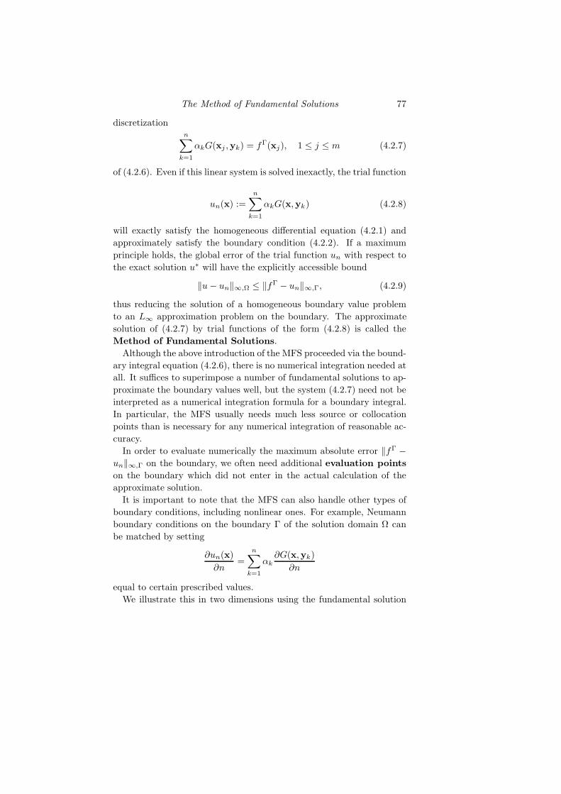
The Method of Fundamental Solutions 77
discretizationn∑
k=1
αkG(xj ,yk) = fΓ(xj), 1 ≤ j ≤ m (4.2.7)
of (4.2.6). Even if this linear system is solved inexactly, the trial function
un(x) :=n∑
k=1
αkG(x,yk) (4.2.8)
will exactly satisfy the homogeneous differential equation (4.2.1) and
approximately satisfy the boundary condition (4.2.2). If a maximum
principle holds, the global error of the trial function un with respect to
the exact solution u∗ will have the explicitly accessible bound
‖u− un‖∞,Ω ≤ ‖fΓ − un‖∞,Γ, (4.2.9)
thus reducing the solution of a homogeneous boundary value problem
to an L∞ approximation problem on the boundary. The approximate
solution of (4.2.7) by trial functions of the form (4.2.8) is called the
Method of Fundamental Solutions.
Although the above introduction of the MFS proceeded via the bound-
ary integral equation (4.2.6), there is no numerical integration needed at
all. It suffices to superimpose a number of fundamental solutions to ap-
proximate the boundary values well, but the system (4.2.7) need not be
interpreted as a numerical integration formula for a boundary integral.
In particular, the MFS usually needs much less source or collocation
points than is necessary for any numerical integration of reasonable ac-
curacy.
In order to evaluate numerically the maximum absolute error ‖fΓ −un‖∞,Γ on the boundary, we often need additional evaluation points
on the boundary which did not enter in the actual calculation of the
approximate solution.
It is important to note that the MFS can also handle other types of
boundary conditions, including nonlinear ones. For example, Neumann
boundary conditions on the boundary Γ of the solution domain Ω can
be matched by setting
∂un(x)
∂n=
n∑
k=1
αk∂G(x,yk)
∂n
equal to certain prescribed values.
We illustrate this in two dimensions using the fundamental solution

78
G(x,y) = ln(‖x − y‖2) of the Laplace operator L = ∆ which, remark-
ably, is another radial basis function. Let
p = (p1, p2),q = (q1, q2), r = ‖p− q‖2 =√
(p1 − q1)2 + (p2 − q2)2
and let p be on the boundary Γ with a unit normal n = (n1, n2) at p.
Then
∂G(p, ·)∂n
(q) =∂
∂nln r =
1
r
(∂r
∂q1n1 +
∂r
∂q2n2
)
=1
r2((p1 − q1)n1 + (p2 − q2)n2)
(4.2.10)
See Figure 4.1 for illustration.
p
q
n(p)
r(p,q)
p1 - q1
p2 - q2
Fig. 4.1. Source point and its boundary nodal point.
In the following, we shall give a more detailed mathematical anal-
ysis and a density-based convergence argument. Application-oriented
readers may skip to Section 4.4 from here.
Assume that ϕℓ(y)∞ℓ=1 is a complete set of functions on Γ. Then
the source distribution σ of (4.2.3) can be well approximated by trial
functions
σL(y) =
L∑
ℓ=1
cℓϕℓ(y), y ∈ Γ. (4.2.11)
This means that we can find a sufficiently large L and coefficients cℓsuch that
‖σ − σL‖∞,Γ =
∥∥∥∥∥σ(y) −L∑
ℓ=1
cℓϕℓ(y)
∥∥∥∥∥∞,Γ
≤ ǫ (4.2.12)
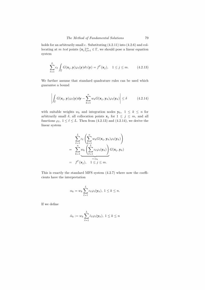
The Method of Fundamental Solutions 79
holds for an arbitrarily small ǫ. Substituting (4.2.11) into (4.2.6) and col-
locating at m test points xjmj=1 ∈ Γ, we should pose a linear equation
system
L∑
ℓ=1
cℓ
∫
Γ
G(xj ,y)ϕℓ(y)dγ(y) = fΓ(xj), 1 ≤ j ≤ m. (4.2.13)
We further assume that standard quadrature rules can be used which
guarantee a bound
∣∣∣∣∣
∫
Γ
G(xj ,y)ϕℓ(y)dy −n∑
k=1
wkG(xj ,yk)ϕℓ(yk)
∣∣∣∣∣ ≤ δ (4.2.14)
with suitable weights wk and integration nodes yk, 1 ≤ k ≤ n for
arbitrarily small δ, all collocation points xj for 1 ≤ j ≤ m, and all
functions ϕℓ, 1 ≤ ℓ ≤ L. Then from (4.2.13) and (4.2.14), we derive the
linear system
L∑
ℓ=1
cℓ
(n∑
k=1
wkG(xj ,yk)ϕℓ(yk)
)
=
n∑
k=1
wk
(L∑
ℓ=1
cℓϕℓ(yk)
)
︸ ︷︷ ︸=:αk
G(xj ,yk)
= fΓ(xj), 1 ≤ j ≤ m.
This is exactly the standard MFS system (4.2.7) where now the coeffi-
cients have the interpretation
αk = wk
L∑
ℓ=1
cℓϕℓ(yk), 1 ≤ k ≤ n.
If we define
αk := wk
L∑
ℓ=1
cℓϕℓ(yk), 1 ≤ k ≤ n

80
with the coefficients of (4.2.12), we find∣∣∣∣∣
n∑
k=1
αkG(xj ,yk) − fΓ(xj)
∣∣∣∣∣
=
∣∣∣∣∣
L∑
ℓ=1
cℓ
n∑
k=1
wkG(xj ,yk)ϕℓ(yk) − fΓ(xj)
∣∣∣∣∣
≤∣∣∣∣∣
L∑
ℓ=1
cℓ
∫
Γ
G(xj ,y)ϕℓ(y)dy − fΓ(xj)
∣∣∣∣∣+ δ‖c‖∞
≤∣∣∣∣∫
Γ
G(xj ,y)σL(y)dy −∫
Γ
G(xj ,y)σ(y)dy
∣∣∣∣ + δ‖c‖∞
≤ ǫ
∫
Γ
|G(xj ,y)|dy + δ‖c‖∞
and see that the MFS system (4.2.7) has a good approximate solution
under the above hypotheses. This means that for sufficiently dense test
points and source points, and for sufficiently smooth boundary functions,
the MFS system can be expected to be solvable by a regularized least-
squares solver, and the error in the system can be made arbitrarily small.
If, finally, the actual error∣∣∣∣∣
n∑
k=1
αkG(x,yk) − fΓ(x)
∣∣∣∣∣
for the calculated coefficients αk is evaluated on the boundary, and if a
maximum principle holds, users have sharp and arbitrarily small bounds
on the total error. This argument applies to most of the examples in
this chapter.
But users should note that the above analysis uses an unrealistically
large number of source points yk, because they are chosen to supply a
good integration formula on the fictitious boundary. A much smaller
number may be sufficient to achieve a small error in the approximation
on the boundary, as described by (4.2.9). This is supported by the
many examples of this chapter. Unfortunately, the approximation power
of traces of fundamental solutions on boundary curves or surfaces is a
difficult theoretical problem still under investigation.
4.3 Fundamental Solutions
Table 4.1 lists fundamental solutions of some commonly used linear dif-
ferential operators which will frequently occur in later sections or chap-

The Method of Fundamental Solutions 81
ters. Since all of these operators are radially invariant, their fundamental
solutions are radial kernels G(x,y) = γ(‖x− y‖2), and we only have to
list scalar radial basis functions γ of the argument r := ‖x − y‖2.
L γ(r) in IR2 γ(r) in IR3
∆−1
2πln r
1
4πr
∆2 −1
8πr2 ln r
r
8π
∆ − λ2 1
2πK0(λr)
e−λr
4πr
∆ + λ2 i
4H
(2)0 (λr)
e−iλr
4πr
(∆ − λ2
)2 −r
4πλK1 (λr) −
e−λr
8πλ
∆(∆ − λ2
) −1
2πλ2(K0 (λr) + ln r) −
e−λr − 1
4πλ2r
∆2 − λ4 1
8λ2
(−iH
(1)0 (λr) +
2
πK0(λr)
)e−λr + e−iλr
4πλ2
Table 4.1. Fundamental solutions for various differential operators.
In Table 4.1, K0 and K1 denote modified Bessel functions of second
kind, while H(2)0 is the Hankel function of order zero, and i =
√−1 as
usual.
For the fundamental solutions of the product of Helmholtz operators,
we refer readers to the Reference [CAO94].
4.4 Static Implementation
It is an important issue to determine the optimal location of the ficti-
tious boundary. In general, there are two different approaches in the
literature: static and dynamic. A third technique is also proposed in
this book, combining these two approaches. We shall treat these three
approaches in separate sections, starting with the static approach.
In the static approach, the source locations yknk=1 are chosen a-
priori in some fashion. Bogomolny [Bog85] and Cheng [Che87] have
laid the theoretical foundations in this direction. In both papers, the

82
fictitious boundary was chosen to be a circle in 2D and a sphere in 3D
with center located at the centroid of the solution domain. In fact, the
numerical results for problems with smooth domains and smooth solu-
tions reveal that the shape of the fictitious boundary has only a small
effect on the results, as long as it stays well away from the boundary
of the solution domain. As a result, it is convenient to generate the
source points uniformly distributed on a circle or sphere. Thus, in our
two-dimensional numerical examples that we show later, we will mostly
choose circles as fictitious boundaries. Theoretically, the optimal choice
of the fictitious boundary is a circle or sphere with infinite radius under
certain assumptions eliminating cases with singularities. But since the
resulting problems become more and more ill–conditioned when the fic-
titious boundary moves out to infinity, the radius should be chosen as
large as to make the systems still solvable on a given computer precision,
as suggested by Bogomolny [Bog85]. However, users must be aware that
the numerical solution will always extend out to the fictitious boundary,
and this rules out problems where singularities of the solution on the
boundary can be expected, e.g. for elliptic problems on domains with
incoming corners and general boundary data. See Section 4.8.2 for an
example.
Cheng’s result [Che87] was generalized by Katsurada and Okamoto
[Kat90, Kat94, KO88, KO96], who showed that if Γ is a closed Jordan
curve in the plane and the data are analytic, then
‖u− un‖∞,Γ ≤ c( rR
)n
where c is a constant, r and R are the diameters of Γ and Γ, respectively.
Once the source points are chosen on Γ, the coefficients αknk=1 in
(4.2.8) can be obtained by either least-squares or collocation methods.
For least-squares,m ≥ n test or collocation points xjmj=1 are chosen
on Γ and then αknk=1 are chosen to minimize [Bog85]
m∑
j=1
(n∑
k=1
αkG(xj ,yk) − fΓ(xj)
)2
in a least squares sense. Note that this was the suggestion for solving the
non-quadratic asymmetric system (4.2.7) of Section 4.2 approximately.
For collocation, the number n of source points on the fictitious bound-
ary and the numberm of test points on the physical boundary are chosen
to be equal, so that (4.2.7) becomes a quadratic symmetric linear system

The Method of Fundamental Solutions 83
of equations
n∑
k=1
αkG(xj ,yk) = fΓ(xj), 1 ≤ j ≤ n. (4.4.1)
In view of the maximum principle and for getting an optimal error
bound in the sense of (4.2.9), the optimal way to handle (4.2.7) is to take
m very large and to calculate the coefficients that solve this overdeter-
mined system by minimizing not the sum of squares, but the maximum
of the absolute values of the residuals. This can be rewritten as a linear
optimization algorithm and solved efficiently by the dual revised simplex
method.
Due to the density results shown in [Bog85], we generally need to add
a constant to (4.4.1) for the Laplace equation. This means that
un(x) =
n∑
k=1
αkG(x,yk) + α0, x ∈ Ω.
In this case, we have to collocate n + 1 points xjnj=0 on the physical
boundary and n source points yknk=1 on Γ. This gives the system
n∑
k=1
αkG(xj ,yk) + α0 = g(xj), 0 ≤ j ≤ n. (4.4.2)
Of course, a similar addition can be made when solving (4.2.7) approx-
imately by minimizing minimizing the sum of squares or the maximum
of the residuals.
In [Bog85], the author also investigated the influence of the inclusion
of a constant function into the set of trial functions. It was found that
the difference between (4.4.1) and (4.4.2) is perceptible only when the
fictitious boundary is close to the physical boundary. Hence, for con-
venience, we use (4.4.1) throughout in the next few sections for solving
the Laplace equation. For other differential equations, α0 in (4.4.2) is
not required.
For domains with interior holes, additional source points should be
placed inside the holes as shown in Figure 4.2.
The following examples are given to illustrate the effectiveness of the
method of fundamental solutions described above. We proceed from
rather simple examples to more complicated application-oriented ones.
Example 4.4.3 Here, we present a benchmark case considered by Fen-

84
Fig. 4.2. The location of sources points.
2y
π=
x=1u’=0
u=0
u =
eco
s(y)
u =
cos(
y)
•( )1/ 2, / 4π
Fig. 4.3. The rectangular domain and boundary conditions.
ner [Fen91]. The governing equation is the homogeneous Laplace op-
erator, and the appropriate fundamental solution is the singular radial
basis function φ(r) = ln r. As shown in Figure 4.3, the boundary condi-
tions prescribe a potential on three sides of the domain, and a potential
gradient on the fourth. The exact solution is u∗(x, y) = ex cos y, causing
no problems when source points are far away from the domain. The
contour plot of the exact solution is shown in Figure 4.4. As indicated
in [Fen91], the problem is considered as one of moderate complexity
and has been used before as an example for testing an Hermitian cubic
boundary element formulation.
Let n = 20 be the number of collocation points which are uniformly
distributed on the physical boundary and let the same number of sources
be uniformly distributed on a circle with center at (0.5, π/4) and radius

The Method of Fundamental Solutions 85
1
2
3
4
4
5
5
6
6
6
7
7
8
8
910
1011
12
1314
15
X
Y
0 0.5 1 1.50
0.2
0.4
0.6
0.8
1
1.2
1.4 Level a15 2.548414 2.378513 2.208612 2.038711 1.868810 1.69899 1.5298 1.35917 1.18926 1.01935 0.8494014 0.6795023 0.5096022 0.3397021 0.169802
1
1
2
2
3
6 8
X
Y
0 0.5 1 1.50
0.2
0.4
0.6
0.8
1
1.2
1.4 Level b15 2.47735E-0714 2.3122E-0713 2.14705E-0712 1.9819E-0711 1.81674E-0710 1.65159E-079 1.48644E-078 1.32129E-077 1.15614E-076 9.90989E-085 8.25838E-084 6.60687E-083 4.95536E-082 3.30385E-081 1.65234E-08
Fig. 4.4. The contour of exact solution of u (left) and its absolute error (right).
2. The contour plots of the absolute errors of u − un, ∂u/∂x− ∂un/∂x
and ∂u/∂y− ∂un/∂y are shown in Figures 4.4 to 4.5.
1
1
1
2
2
3
5
14
X
Y
0 0.5 1 1.50
0.2
0.4
0.6
0.8
1
1.2
1.4 Level c15 1.99228E-0614 1.85947E-0613 1.72665E-0612 1.59383E-0611 1.46102E-0610 1.3282E-069 1.19538E-068 1.06257E-067 9.29749E-076 7.96932E-075 6.64116E-074 5.31299E-073 3.98482E-072 2.65665E-071 1.32849E-07
1
1
1
1
1
1
2
2
2
3
3
4
4
5
5
67
1114
X
Y
0 0.5 1 1.50
0.2
0.4
0.6
0.8
1
1.2
1.4 Level d15 1.38628E-0614 1.29386E-0613 1.20145E-0612 1.10903E-0611 1.01661E-0610 9.24194E-079 8.31777E-078 7.39359E-077 6.46941E-076 5.54524E-075 4.62106E-074 3.69688E-073 2.77271E-072 1.84853E-071 9.24355E-08
Fig. 4.5. The contour of absolute error ∂u∂x
(left) and ∂u∂y
(right).
We observe that the maximum errors of u, ∂u/∂x, and ∂u/∂y occur
near the corners where the boundary condition changes from a Dirichlet
condition to a Neumann condition. The absolute maximum errors of u,
∂u/∂x, and ∂u/∂y evaluated at 400 boundary points are shown in Table
4.2 as functions of the radius R of the fictitious boundary circle. The
accuracy is relatively independent of R in this example. 2
Example 4.4.4 We consider a bounded domain Ω with an irregular

86
R ‖u− un‖∞ ‖∂u/∂x− ∂un/∂x‖∞ ‖∂u/∂y − ∂un/∂y‖∞
2.5 1.18E−7 1.21E−6 7.40E−6
4.0 3.03E−7 2.46E−6 1.70E−6
8.0 2.04E−7 2.13E−6 1.48E−6
12 2.41E−7 1.93E−6 1.34E−6
15 2.34E−7 1.88E−6 1.31E−6
18 2.28E−7 1.84E−6 1.28E−6
Table 4.2. Maximum absolute errors of u, ∂u∂x , and ∂u
∂y .
boundary ∂Ω = ΓD ∪ ΓN and the mixed boundary conditions
∆u = 0, (x1, x2) ∈ Ω,
u = ex1 cosx2, (x1, x2) ∈ ΓD,∂u
∂n= ex1(cos x2nx1 − sinx2nx2), (x1, x2) ∈ ΓN ,
where (nx1 , nx2) is a unit normal vector and
∂Ω =(r cos θ, r sin θ) : r = esin θ sin2 2θ + ecos θ cos2 2θ, 0 ≤ θ ≤ 2π
.
Then ΓD is the upper half curve of ∂Ω with 0 ≤ θ < π and ΓN is the
−1.5 −1 −0.5 0 0.5 1 1.5 2 2.5 3−1.5
−1
−0.5
0
0.5
1
1.5
2
ΓD
X
Y
ΓN
Ω
Fig. 4.6. The profile of an amoeba-like boundary.
lower half curve with π ≤ θ < 2π. The exact solution is given by the
global function u∗(x1, x2) = ex1 cosx2 such that the incoming corners
and the change of boundary conditions induce no boundary singularities.

The Method of Fundamental Solutions 87
n ‖u− un‖∞ ‖∂u/∂x1 − ∂un/∂x1‖∞ ‖∂u/∂x2 − ∂un/∂x2‖∞
120 5.755E−12 6.124E−11 3.072E−10
140 5.960E−13 1.078E−11 1.147E−11
160 9.470E−14 1.794E−12 9.325E−13
180 1.303E−13 1.239E−12 1.498E−12
200 1.569E−13 1.545E−12 1.840E−12
220 7.761E−13 5.818E−12 5.356E−12
Table 4.3. Absolute maximum solutions of u, ∂u/∂x1, and ∂u/∂x2.
For the numerical implementation, n evenly distributed collocation
points (in term of the angle parametrization) were chosen on the bound-
ary ∂Ω. Figure 4.6 shows the profile of the amoeba-like boundary. The
fictitious boundary is chosen to be a circle with radius 5 and center at
the origin.
To show the numerical results, we chose 61 evenly distributed points
on the physical boundary for testing. The approximate solution and
derivatives are denoted by un, ∂un/∂x1, and ∂un/∂x2 respectively. Ta-
ble 4.3 shows the absolute maximum errors of u, ∂u/∂x1, and ∂u/∂x2
for various n.
2
Example 4.4.5 We consider
∆u = 0, (x1, x2) ∈ Ω,
u = sinx1 coshx2, (x1, x2) ∈ Γ,(4.4.6)
on a multi-connected domain defined by
Ω∪Γ = (x1, x2) :x2
1
4+x2
2 ≤ 1, (x1 − 1)2 +x22 ≥ 1
4, (x1 +1)2 +x2
2 ≥ 1
4,
where Γ consists of an ellipse and two circles as shown in Figure 4.7.
The analytic solution is
u∗ = sinx1 coshx2,
We perform two numerical tests in this example. In both tests, we
chose 40 collocation points on Γ as shown in Figure 4.7. In Test 1, we
chose all the 40 source points outside the solution domain. In Test 2

88
Fig. 4.7. Distribution of collocation points.
we used 20 source points located on a circle with radius R and center
at (0, 0) outside the solution domain and 10 source points with radius
r = 0.4 and center at (0, 1) and (0,−1) inside each circle. The maximum
absolute error of u for various R are shown in Table 4.4. The numerical
results reveal that Test 1 is more accurate and Test 2 is less insensitive
to the the location of source points outside the ellipse. It seems that
our test contradicts the results shown in [Fen91] which indicated that
the strategy of using a single source circle enclosing the domain may not
give satisfactory results. 2
Test 1 Test 2 (r = 0.4)
R = 5 1.94E−7 5.68E−6
R = 7 4.62E−9 5.87E−6
R = 9 8.14E−11 4.96E−6
R = 11 5.61E−10 4.29E−6
R = 13 2.71E−8 5.64E−6
R = 15 1.57E−8 3.56E−6
Table 4.4. Absolute maximum error on a multi-connected domain.
In this and several following examples, we consider the Helmholtz
equation(∆ + k2
)u(x) = 0, x ∈ Ω,
which often arises in the study of physical problems involving partial
differential equations. This equation generalizes the standard ordinary

The Method of Fundamental Solutions 89
differential equation
u′′(x) + k2u(x) = 0, x ∈ IR
for stationary waves with solutions cos kx, sinkx, where k is called the
wave number related to the frequency λ by k = 2π/λ. It arises from
the standard technique of separation of variables applied to the wave
equation
∆u(x, t) − 1
c2∂2u
∂t2(x, t) = 0,
because general waves can usually be superimposed from stationary
waves. This reduces solving the time-dependent wave equation to solv-
ing a sequence of spatial Helmholtz equations. Similarly, we shall apply
various techniques to reduce time–dependent problems to a series of
Helmholtz equations in Chapter 6. Hence, it is important to show the
effectiveness of the method of fundamental solutions for solving this type
of equation. Note that the equation is not elliptic unless it is rewritten
for purely imaginary k as
−∆u(x) + γu(x) = 0, x ∈ Ω
for nonnegative γ ∈ IR.
Example 4.4.7 Consider the special Helmholtz equation(−∆ +
π2
2
)u = 0, (x1, x2) ∈ Ω,
u = sinh(πx1
2
)cosh
(πx2
2
), (x1, x2) ∈ Γ,
where Ω ∪ Γ =(x1, x2) : x2
1 + x22 ≤ 4
. The exact solution is given by
u∗ = sinh(πx1
2
)cosh
(πx2
2
),
and the fundamental solution is φ(r) = K0(πr/√
2) (see Table 4.1).
The circle around (0, 0) with radius 5 is the fictitious boundary Γ on
which various numbers of uniformly distributed source points were cho-
sen. The same number of collocation points was chosen on the boundary.
The numerical error was calculated at 400 uniformly distributed eval-
uation points on the domain boundary. Absolute maximum errors for
various numbers of source points are shown in Table 4.5. Note that the
errors decrease rapidly when n becomes larger. When n is sufficiently
large, the error started to decrease due to ill–conditioning. 2
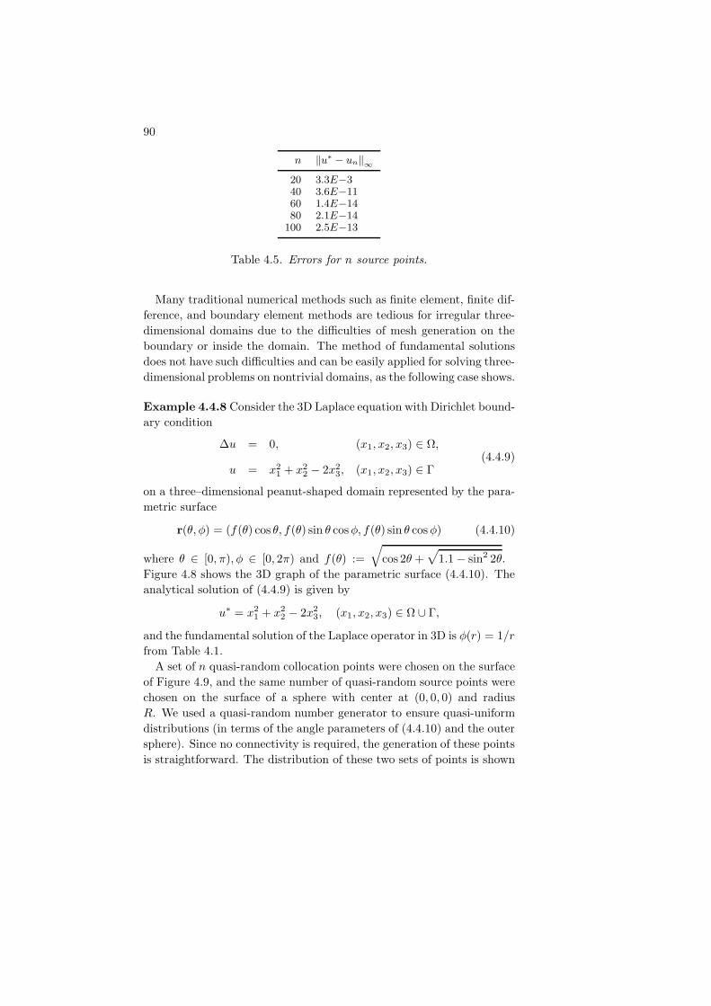
90
n ‖u∗ − un‖∞
20 3.3E−340 3.6E−1160 1.4E−1480 2.1E−14
100 2.5E−13
Table 4.5. Errors for n source points.
Many traditional numerical methods such as finite element, finite dif-
ference, and boundary element methods are tedious for irregular three-
dimensional domains due to the difficulties of mesh generation on the
boundary or inside the domain. The method of fundamental solutions
does not have such difficulties and can be easily applied for solving three-
dimensional problems on nontrivial domains, as the following case shows.
Example 4.4.8 Consider the 3D Laplace equation with Dirichlet bound-
ary condition
∆u = 0, (x1, x2, x3) ∈ Ω,
u = x21 + x2
2 − 2x23, (x1, x2, x3) ∈ Γ
(4.4.9)
on a three–dimensional peanut-shaped domain represented by the para-
metric surface
r(θ, φ) = (f(θ) cos θ, f(θ) sin θ cosφ, f(θ) sin θ cosφ) (4.4.10)
where θ ∈ [0, π), φ ∈ [0, 2π) and f(θ) :=
√cos 2θ +
√1.1 − sin2 2θ.
Figure 4.8 shows the 3D graph of the parametric surface (4.4.10). The
analytical solution of (4.4.9) is given by
u∗ = x21 + x2
2 − 2x23, (x1, x2, x3) ∈ Ω ∪ Γ,
and the fundamental solution of the Laplace operator in 3D is φ(r) = 1/r
from Table 4.1.
A set of n quasi-random collocation points were chosen on the surface
of Figure 4.9, and the same number of quasi-random source points were
chosen on the surface of a sphere with center at (0, 0, 0) and radius
R. We used a quasi-random number generator to ensure quasi-uniform
distributions (in terms of the angle parameters of (4.4.10) and the outer
sphere). Since no connectivity is required, the generation of these points
is straightforward. The distribution of these two sets of points is shown

The Method of Fundamental Solutions 91
Fig. 4.8. Peanut-shaped domain.
-1
0
1-0.5-0.2500.250.5-0.5
-0.25
0
0.25
0.5
-1
0
1
-0.5
-0.25
0
0.25
Fig. 4.9. Collocation points on the boundary.
in Figure 4.10. The absolute maximum errors for various n and R are
shown in Table 4.6. The accuracy is rapidly improving with increasing
n and R.
2
This example shows that flat analytic radial basis functions, if superim-
posed properly, and even if they are singular outside the domain, can
recover multivariate polynomials well. This is another example of the
fact mentioned in Section 2.6, namely that analytic radial basis function
interpolants often converge towards polynomials in their “flat limit”.

92
n = 50 n = 100 n = 150 n = 200
R = 4 1.25E−3 2.79E−9 4.07E−12 1.64E−13
R = 6 5.74E−4 1.28E−11 5.83E−13 3.66E−13
R = 8 7.87E−6 1.48E−12 8.91E−13 3.34E−13
R = 10 1.76E−6 1.64E−12 2.74E−13 6.66E−13
Table 4.6. Absolute maximum errors for various of n and R
Fig. 4.10. The distribution of collocation points and source points.
4.5 Interlude: Stability Issues
It must be expected that the condition numbers of (4.4.1) and (4.4.2)
rapidly deteriorates as the radius R of the fictitious boundary circle or
sphere increases. Despite this ill–conditioning, a greater distance of the
source points yjMj=1 from the boundary Γ will improve the quality of
the approximation of the solution [Bog85] if the boundary is sufficiently
smooth and the given boundary data are exact. This is a curious fea-
ture of the method which has puzzled many researchers, but it is in line
with the observations described in Section 2.4, because the usual linear
systems arising in RBF-based methods have the property that the right-
hand sides usually are close to the span of the columns of the matrix.

The Method of Fundamental Solutions 93
Consequently, optimization methods or singular value decompositions
like those described in Section 2.5 and 2.9 will help to overcome stabil-
ity problems, independent of the actual value of the condition number.
The latter measures the blow-up of relative errors in the coefficients, but
the coefficients are much less relevant than the error committed in repro-
ducing the right-hand side of the system by the constructed approximate
solution.
Also in case of the method of fundamental solutions, the coefficients
αjnj=1 in (4.2.8) are usually not of independent interest, but rather
the approximation quality of the numerical solution
un(x) =
n∑
j=1
αjG(x,yj).
The crucial point is how data errors are amplified in un(x), not neces-
sarily in αjnj=1.
Despite the notorious ill–conditioning problem, the method of funda-
mental solutions can still produce extremely accurate results, because
the Uncertainty Principle for radial basis function approximations
described in Section 2.4 can also be observed in the method of funda-
mental solutions. Subject to machine precision, the worse the condition
numbers, the better the approximate solution. As we shall see in the
following example, the Method of Fundamental Solutions can cope with
large condition numbers, if suitable projections or approximations are
used.
Example 4.5.1 To show how the number of collocation points and the
location of source points on the fictitious boundary affect the solution
of the MFS, we consider the Laplace equation with Dirichlet boundary
conditions as in (4.4.6) and boundary conditions
u = sinx1 coshx2, (x1, x2) ∈ Γ,
where the domain is
Ω ∪ Γ = (x1, x2) :x2
1
4+ x2
2 ≤ 1.
The numerical evaluation of the error was performed using 276 uniformly
distributed evaluation points on the boundary. For various numbers n of
source and collocation points, Figure 4.11 shows the absolute maximum
errors as functions of the radii of the fictitious boundary circles, while
the condition numbers for various radii and source points are shown
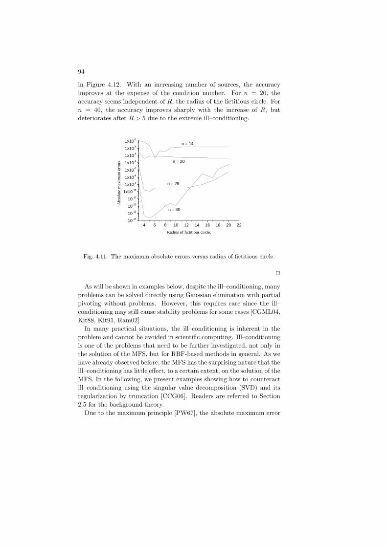
94
in Figure 4.12. With an increasing number of sources, the accuracy
improves at the expense of the condition number. For n = 20, the
accuracy seems independent of R, the radius of the fictitious circle. For
n = 40, the accuracy improves sharply with the increase of R, but
deteriorates after R > 5 due to the extreme ill–conditioning.
4 6 8 10 12 14 16 18 20 2210-14
10-13
10-12
10-11
1x10⁻¹⁰
1x10⁻⁹
1x10⁻⁸
1x10⁻⁷
1x10⁻⁶
1x10⁻⁵
1x10⁻⁴
1x10⁻³
n = 40
n = 29
n = 20
n = 14
Abs
olut
e m
axim
um e
rror
s
Radius of fictitious circle.
Fig. 4.11. The maximum absolute errors versus radius of fictitious circle.
2
As will be shown in examples below, despite the ill–conditioning, many
problems can be solved directly using Gaussian elimination with partial
pivoting without problems. However, this requires care since the ill–
conditioning may still cause stability problems for some cases [CGML04,
Kit88, Kit91, Ram02].
In many practical situations, the ill–conditioning is inherent in the
problem and cannot be avoided in scientific computing. Ill–conditioning
is one of the problems that need to be further investigated, not only in
the solution of the MFS, but for RBF-based methods in general. As we
have already observed before, the MFS has the surprising nature that the
ill–conditioning has little effect, to a certain extent, on the solution of the
MFS. In the following, we present examples showing how to counteract
ill–conditioning using the singular value decomposition (SVD) and its
regularization by truncation [CCG06]. Readers are referred to Section
2.5 for the background theory.
Due to the maximum principle [PW67], the absolute maximum error

The Method of Fundamental Solutions 95
4 6 8 10 12 14 16 18 20103
105
107
109
1011
1013
1015
1017
1019
n = 14
n = 20
n = 29
n = 40
Con
ditio
n N
umbe
rs
Radius of Fictitious Circle
Fig. 4.12. Condition numbers versus the radius of the fictitious boundary cir-cle.
for solutions of the Dirichlet problem for the Laplace equation occurs on
the boundary. Hence, through the next three examples, we calculated
the boundary error using 121 evaluation points that were uniformly dis-
tributed on Γ. Then we chose n < 121 collocation points and source
points which were uniformly distributed (in terms of angles) on the phys-
ical boundary and the fictitious boundary, respectively. Furthermore, we
chose a circle with center at (0, 0) and radius R as the fictitious bound-
ary. We denote by e, ex1 , ex2 the absolute maximum errors of u and
∂u/∂x1 and ∂u/∂x2, respectively; i.e. ,
e = ‖u− un‖∞ , ex1 =
∥∥∥∥∂u
∂x1− ∂un
∂x1
∥∥∥∥∞, ex2 =
∥∥∥∥∂u
∂x2− ∂un
∂x2
∥∥∥∥∞.
Example 4.5.2 Consider the Laplace equation with the following Dirich-
let boundary conditions
∆u = 0, (x1, x2) ∈ Ω
u = sinx1 coshx2, (x1, x2) ∈ Γ,
where
Γ =
(r cos θ, r sin θ) : r =
√cos 2θ +
√1.1 − sin2 2θ, 0 ≤ θ ≤ 2π
.
The exact solution is given by u∗ = sinx1 coshx2.

96
First, we chose 50 collocation and source points on Γ and the fictitious
boundary, respectively. Let R denote the radius of the fictitious circle.
In Table 4.7, we show the absolute maximum errors using SVD and
Gaussian elimination. In the SVD, we used all 50 singular values. We
found that the numerical results using these two approaches showed
practically no difference. There is no evidence that the SVD is superior
to Gaussian elimination here, as can be expected in all numerically stable
cases. 2
SVD Gaussian
R e ex1 e ex1
4 9.00E − 9 1.35E − 7 2.78E − 8 4.84E − 7
6 7.83E − 10 1.13E − 8 4.33E − 10 6.44E − 9
8 1.70E − 10 2.88E − 9 24.25E − 10 7.18E − 9
Table 4.7. Comparison of Gaussian elimination and SVD using 50
collocation and source points.
Example 4.5.3 We consider Laplace equation with mixed boundary
conditions. Let Γ = ΓD ∪ ΓN . As shown in Figure 4.13, we imposed
a Dirichlet condition on ΓD, which contains the upper half of Γ, and
a Neumann condition on ΓN , which contains the lower half of Γ. The
boundary conditions are imposed in such a way that the exact solution
still is u∗ = sinx1 coshx2.
We chose 200 collocation and source points and performed the same
tests as shown in Example 4.5.2. Again, as displayed in Table 4.8, the
results do not indicate that the SVD is superior to Gaussian elimination.
For testing the truncated singular value decomposition (TSVD)
described in Section 2.5, we chose the first 50 singular values and con-
ducted the same numerical tests as above. The numerical results in
Table 4.9 show that there are no differences for R = 4. However, the
numerical results are more stable when R increases. This indicates that
the TSVD is superior to the SVD in terms of accuracy and efficiency for
using large numbers of collocation and source points. We will further
elaborate on this observation in the next two examples.
2

The Method of Fundamental Solutions 97
−2 −1.5 −1 −0.5 0 0.5 1 1.5 2−0.8
−0.6
−0.4
−0.2
0
0.2
0.4
0.6
0.8
x1
x 2
ΓD
ΓN
Ω
Fig. 4.13. Profile of the Neumann and Dirichlet boundary conditions.
SVD Gaussian
R e ex1 e ex1
4 6.47E − 14 2.07E − 13 5.05E − 14 3.91E − 13
6 1.34E − 12 1.80E − 12 5.00E − 13 1.95E − 12
8 5.42E − 10 4.29E − 9 5.42E − 10 4.29E − 9
Table 4.8. Absolute maximum errors e and ex1 for mixed boundary
conditions.
Example 4.5.4 To study the effect of the TSVD on the accuracy, we
consider again the Laplace equation with mixed boundary conditions.
Let
Γ = (r cos θ, r sin θ) : r = esin θ(sin2(2θ)) + ecos θ(cos2(2θ)).
The boundary Γ is an amoeba-like irregular shape, see Figure 4.14. The
boundary conditions are given by
∂u
∂n= (cosx1 coshx2)nx1 + (sinx1 sinhx2)nx2 , (x1, x2) ∈ ΓN ,
u = sinx1 coshx2, (x1, x2) ∈ ΓD,

98
TSVD
R e ex1
4 3.96E − 14 1.72E − 13
6 8.45E − 14 1.67E − 13
8 1.35E − 12 1.67E − 12
Table 4.9. Absolute maximum errors e and ex1 for mixed boundary
conditions.
where (nx1 , nx2) is a unit normal vector, ΓN = Γ with 0 ≤ θ < π/2,
and ΓD = Γ with π/2 ≤ θ < 2π. The exact solution is given by
u∗ = sinx1 coshx2. As shown in Figure 4.14, the Neumann condition is
imposed on the first segment of the amoeba-like curve, and the Dirichlet
boundary condition on the rest of Γ.
−2 −1 0 1 2 3−1.5
−1
−0.5
0
0.5
1
1.5
2
ΓD
ΓN
x1
x 2
Fig. 4.14. Neumann and Dirichlet boundary conditions.
We first chose 200 collocation and source points on Γ and the fictitious
circle with R = 4, respectively. In Figure 4.15, we show the absolute
maximum errors of e, ex1, and ex2 versus the number of singular values
being used. In Figure 4.15, we also present the distribution of the singu-
lar values. There seems to be no significant difference in accuracy when

The Method of Fundamental Solutions 99
using more than 50 singular values. This indicates that the truncation
error and round off error have little effect on the accuracy, but users are
advised not to use more singular values than necessary.
Table 4.10 shows again that there is no significant difference between
Gaussian elimination and SVD using 200 collocation and source points.
We have conducted several tests using various boundary shapes and
conditions, and found no significant difference, even for mixed boundary
conditions, when using a circle as the fictitious boundary.
40 60 80 100 120 140 160 180 20010
−14
10−13
10−12
10−11
10−10
10−9
10−8
10−7
Number of Singular Values
Ab
solu
te M
axi
mu
m E
rro
rs
e e
xe
y
0 20 40 60 80 100 120 140 160 180 200
10−15
10−10
10−5
100
Number of Singular Values
Sin
gula
r V
alue
s
Fig. 4.15. Numerical results of e, ex1 , ex2 (upper graph) and distribution ofsingular values (lower graph) using 200 collocation and source points.
2
Example 4.5.5 We consider Example 4.5.4 adding random noise to the

100
Source radius R e (Gaussian) e (SVD) e (TSVD)
4 1.27E − 12 2.99E − 13 2.88E − 14
5 8.21E − 14 1.34E − 13 4.90E − 14
6 3.12E − 13 3.01E − 13 2.75E − 13
7 1.46E − 12 1.00E − 11 5.70E − 13
Table 4.10. Comparison of Gaussian elimination, SVD and TSVD.
boundary conditions as
∂u
∂n= (sinx1 coshx2)nx1 + (sinx1 coshx2)nx2 + δ, (x1, x2) ∈ ΓN ,
u = sinx1 coshx2 + δ, (x1, x2) ∈ ΓD,
where δ stands for uniformly distributed random numbers drawn from
[−ε, ε], such that ε denotes the noise level. As in the last example, we
chose 200 collocation and source points. We chose 60 singular values
for the truncated singular-value decomposition (TSVD). The noise level
ε was set to be at 1%. The absolute maximum errors for e, ex1 and
ex2 versus the source radius are shown in Figures 4.16 and 4.17. It is
clear that the TSVD is superior to the SVD and Gaussian elimination.
Again, there is little difference between Gaussian elimination and the
SVD. Note how a careful analysis of the singular values can help to
determine the noise level and the correct number of signgular values to
use. This is in line with the results of Section 2.5 on regularization.
2
In [HW05, Jin04] the authors discussed in detail how to choose cer-
tain regularization parameters using various techniques. However, we
found that the simple truncated singular-value decomposition (TSVD)
is sufficient to produce satisfactory results in our cases, in particular
if condition numbers are extremely large and if there is noise. We sug-
gest choosing a sufficiently large number of collocation and source points
in the formulation and then to comfortably cut-off at least half of the
singular values without loss of accuracy. Using SVD, we know how to
eliminate the smaller singular values, and using TSVD, the radius of the
fictitious circus is no longer a critical issue. This follows since the larger
the radius of the source circle, the worse the ill–conditioning becomes.
However, since the ill–conditioning is caused by the small singular values,

The Method of Fundamental Solutions 101
8 10 12 14 16 18 2010
−2
10−1
100
101
102
e
Source Radius
Abs
olut
e M
axim
um E
rror
sTSVD TSV Gaussian
8 10 12 14 16 18 2010
−2
10−1
100
101
102
ex
Source Radius
Abs
olut
e M
axim
um E
rror
s
TSVD SVD Gauss
Fig. 4.16. Absolute maximum errors of e (above) and ex1 (below).
it is rather easy to remove them in order to have a stable computation.
The price we have to pay for a simple and maybe too large choice of the
source radius is to choose many more source points than needed. In the
last and current example, we found that only 60 out of 200 singular val-
ues are enough to produce accurate results. This is in perfect agreement
with the results of Section 2.5 and the simple example yielding Figure
2.7.
Examples 4.5.2 – 4.5.5 show that the SVD without truncation or regu-
larization does not appear to be more reliable than Gaussian elimination
for solving these equations for non–noisy boundary conditions. Since
Gaussian elimination is cheaper than SVD, it appears that it can be used
to efficiently and accurately implement the MFS. But this requires that

102
8 10 12 14 16 18 2010
−2
10−1
100
101
102
ey
Source Radius
Abs
olut
e M
axim
um E
rror
s
TSVD SVD Gauss
Fig. 4.17. Absolute maximum errors of ex2 .
the numerical routine used for Gaussian elimination be well-programmed
and its pivoting process be cut off properly. Users are discouraged from
using self-made solvers. For noisy data and highly ill–conditioned sit-
uations, the truncated singular-value decomposition (TSVD) is clearly
superior to Gaussian elimination. However, we shall see in Section 4.9
that inverse problems call for even more careful regularization, and then
we shall use the Tikhonov strategy, as described in Section 2.5. Note
that TSVD is considered as a regularization method, not as a plain
solution technique.
4.6 Dynamic Implementation
This approach was first proposed by Mathon and Johnson [MJ77] and
further developed by Fairweather and Karageorghis [FK98] and extended
to a wide variety of problems, see [Kar92, KF87, KF89a, KO88, PKG98],
and references cited therein. In this approach, the locations of n source
points yknk=1 and the corresponding source strength factors αkn
k=1
in (4.2.8) are both treated as unknown and are to be found as part of
the solution. A set of m collocation points xjmj=1 is selected on the
boundary where e.g. a Dirichlet boundary condition is provided by a
known function g. Then the objective function
εm(a,Y) =
m∑
j=1
(un(xj ;a,Y) − g(xj))2
(4.6.1)

The Method of Fundamental Solutions 103
is minimized in a non–linear least-squares sense with respect to a :=
αjnj=1 and Y := yjn
j=1. This is a nonlinear optimization problem
which has high computational cost. There are 3n unknown to be deter-
mined in 2D problems and 4n for 3D problems. Since significantly more
source points are required for the 3D problems, it becomes inefficient in
implementation unless one can get away with very small n, i.e. with a
very well-chosen trial space.
Consider the following biharmonic problem
∆2u = 0, x ∈ Ω, (4.6.2)
subject to either
u = g1(x),∂u
∂n= h1(x), x ∈ Γ,
or
u = g2(x), ∆u = h2(x), x ∈ Γ. (4.6.3)
Karageorghis and Fairweather [KF87] proposed the solution to be ap-
proximated by a linear combination of fundamental solutions of both
the Laplace and biharmonic equations; i.e. ,
un(x) =
n∑
k=1
αkG1(x,yk) +
n∑
k=1
βkG2(x,yk)
where G1 and G2 are the fundamental solutions of ∆ and ∆2, respec-
tively, and where we dropped the dependence of un on the yk and the
coefficients αk, βk. Similar to the formulation of (4.6.1), the approx-
imate solution un must satisfy the biharmonic equation (4.6.2), and
αjnj=1,βjn
j=1 and the positions of the source points yjnj=1 must be
chosen in such a way that the boundary conditions (4.6.3) are satisfied.
To achieve this goal, the following nonlinear functions are minimized
εm =
m∑
j=1
((un − g1(xj))
2 +
(∂un
∂n− h1(xj)
)2)
(4.6.4)
or
εm =
m∑
j=1
((un − g2(xj))
2 + (∆un − h2(xj))2), (4.6.5)
depending on the type of the boundary conditions, and where the source
points and coefficients hidden in un are varying.
The minimization of the functionals in (4.6.1), (4.6.4) or (4.6.5) can
be performed by using various least squares minimization algorithms.

104
Among them, MINPACK, IMSL [IMS01] and NAG [NAG01] are com-
monly used. The routines LMDIF and LMDER from MINPACK mini-
mize the sum of squares of n nonlinear functionals in m variables using
a modified version of the Levenberg–Marquardt algorithm. Users
should be aware that it implicitly uses a regularization strategy which
is similar to Tikhonov regularization. LMDIF evaluates the Jacobian
internally by a forward-difference approximation, whereas LMDER re-
quires the user provide a subroutine that evaluates the Jacobian analyt-
ically. It terminates when either a user-specified tolerance is achieved
or a user-specified maximum number of function evaluations is reached.
The subroutine E04UPF from NAG can also be used. This subroutine
employs a sequential quadratic programming algorithm and minimizes
a functional consisting of a sum of squares. This subroutine can be
used either for unconstrained or constrained optimization. The subrou-
tine E04UPF terminates when a user-specified tolerance is found. The
tolerance can be supplied through an optional input parameter which
specifies the accuracy to which the user wishes the final iterate to ap-
proximate the solution of the problem. The subroutines UNLSF and
UNSLSJ from IMSL can also be used. UNLSF is based on a modified
Levenberg–Marquardt and a finite-difference Jacobian while UNSLSJ
uses the same algorithm with a user-supplied Jacobian. Note that if
the exact Jacobian is supplied in above mentioned subroutines, the ef-
ficiency, as we shall see in the numerical implementation later, will be
significantly improved. However, the complexity of the code will in-
crease, too.
The initial placement of the moving sources and the positioning of
the fixed boundary points are extremely important as they greatly affect
the convergence of the least squares procedure. In general, the sources
are initially distributed uniformly at a fixed distance from the boundary
[KF87], and the boundary points are selected uniformly on the boundary.
Following the recommendation of Oliveira [Oli68], the number m of test
or collocation points on the boundary is chosen to be approximately
three times the number of unknowns determined by the number n of
source points and the space dimension. The tendency of the sources to
move to the interior of the solution domain is overcome by an internal
check of the position of singularities during the iterative process. If a
source is moved inside Ω, it is repositioned at the exterior of the domain
[KF87].
Since the minimization problem of (4.6.4) or (4.6.5) is non–linear,
there is no guarantee that it has a unique global solution, i.e. the solution

The Method of Fundamental Solutions 105
obtained may be just an approximation of a local minimum instead of the
global minimum. Hence, one has to observe convergence using various
parameters and use the algorithms with care.
In the implementation of the MFS, it is often difficult to decide a pri-
ori how many sources and boundary collocation points should be used
in order to fit the boundary condition satisfactorily. MacDonell [Mac85]
introduced the idea of starting with a certain number of sources, say n1,
and a corresponding number of boundary points m1, and after a certain
number of function evaluations, adding sources so that the total num-
ber becomes n2 and the corresponding number of boundary collocation
points is increased to m2, a process which can be repeated until the
desired accuracy is reached. The additional sources are distributed uni-
formly around the region at a user-specified distance along the normal
of the surface. This improved version of the MFS was used in the so-
lution of biharmonic problems [KF87] and produced faster convergence
of the method. However, it reports no improvement for some nonlinear
boundary problems [KF89a].
Example 4.6.6 Consider the harmonic test problem [PKG98]
∆u = 0, (x1, x2) ∈ Ω,
u = x1, (x1, x2) ∈ Γ,
where Ω ∪ Γ = (x1, x2) : −1 ≤ x1, x2 ≤ 1.The sources were initially positioned at uniformly distributed points,
at a fixed distance d = 0.1 from the boundary. In this example, the CPU
time used was measured as a function of the user-specified tolerance ǫ
for ‖u− um‖ ≤ ǫ on the boundary. Let n denote the number of source
points and m the number of collocation points on Γ. All computations
were performed in double precision on an IBM RISC 6000 computer.
The CPU times in seconds for various ǫ,m and n, and for various least
squares software packages are shown in Table 4.11. There, E04UPF*
denotes that the Jacobian was evaluated internally, while E04UPE**
denotes that the Jacobian was provided by the user. From the table we
notice that the CPU times required by using LMDER and E04UPF**
are much less than those of LMDIF and E04UPF**.
2
Example 4.6.7 Consider the biharmonic equation (4.6.2) subject to
the boundary conditions u(x1, x2) = x21 and ∆u(x1, x2) = 2 where Ω∪Γ

106
ǫ m n LMDIF LMDER E04UPF* E04UPF**
10−2 6 56 1.1 0.6 1.4 0.27 64 2.3 1.2 1.3 0.28 72 3.7 2.0 93.1 0.49 84 3.4 1.9 141.2 1.310 92 3.5 3.3 151.8 1.1
10−3 6 56 1.1 0.7 2.6 1.67 64 20.1 1.8 4.3 0.78 72 18.6 10.2 129.6 3.99 84 22.4 12.6 243.4 6.110 92 22.3 15.6 260.0 8.3
10−4 6 56 3.3 0.8 3.7 1.97 64 56.8 56.0 60.3 10.58 72 159.7 93.4 339.9 46.79 84 398.6 146.3 506.4 95.410 92 463.3 178.3 617.7 110.4
Table 4.11. CPU times in seconds required by the least squares
minimization routines.
is the same as in the previous example. This problem is considered by
[PKG98]. The exact solution is u∗(x1, x2) = x21.
The performance of the various routines shown in Table 4.12 is similar
to those for the harmonic problem in the previous example, and the
notations are the same. The relative efficiency of the routines is the
same as above, but the CPU times required in this example are much
higher than in the previous example.
2
Example 4.6.8 In this example we consider
∆u = 0, (x1, x2) ∈ Ω,
u = x21 − x2
2, (x1, x2) ∈ Γ,
where Ω is an ellipse as shown in Example 4.5.1. We used the subrou-
tine DUNLSF from the IMSL library. A total of 72 collocation points
were uniformly distributed on the boundary and 8 source points were
initially placed on a uniformly distributed fictitious boundary ellipse
(3 cos θ, 2 sin θ) : 0 ≤ θ < 2π. The initial values of αjnj=1 were all
set equal to 1. Both the absolute and relative function tolerance are
set equal to 10−5. The numerical computation was performed using 276
evenly distributed points on the boundary. We obtained an absolute

The Method of Fundamental Solutions 107
ǫ m n LMDIF LMDER E04UPF* E04UPF**
10−2 6 72 3.2 1.7 51.4 1.57 84 7.5 4.0 69.2 1.58 96 8.2 4.1 146.7 3.39 108 9.8 5.1 343.2 4.610 120 12.1 6.2 467.9 4.5
10−3 6 72 27.9 15.4 89.4 9.67 84 53.3 30.2 159.7 21.78 96 78.7 39.2 462.7 26.49 108 125.7 64.4 767.3 53.910 120 120.9 60.0 957.4 62.7
10−4 6 72 411.8 352.8 461.4 255.47 84 860.4 274.4 735.6 310.88 96 829.2 427.2 920.7 422.39 108 1153.1 637.2 1541.2 546.410 120 2235.3 544.5 2462.4 601.9
Table 4.12. CPU times in seconds required by the least squares
minimization routines.
maximum error of ‖u− um‖∞ = 2.75E−4. The final locations of the
source points are shown in Figure 4.18. We have tested different initial
values, and found the final locations of the sources to vary greatly. This
is because there are many ways to approximate a quadratic function well
by a few distant fundamental solutions. 2
4.7 Modified Implementation
Each method of the previous two approaches has their advantages and
disadvantages. A modified MFS combining both approaches is pre-
sented. In the dynamic approach, each source contains two unknowns
in 2D (three in 3D) to be determined. As a result, using the nonlin-
ear routines becomes costly. To reduce the number of unknowns, it is
suggested now that the sources are initially fixed on a fictitious circle
in 2D (sphere in 3D) with radius R. Then the dynamic approach is
applied to determine the radius of the circle. In this way, there are only
m+ 1 unknowns for either the 2D or 3D cases. This modified approach
is particularly attractive for the 3D case.
Example 4.7.1 We use the modified approach to compare with the
static approach in Example 4.5.1. The sources initially are located on

108
-5.0 0.0 5.0 10.0 15.0 20.0 25.0
X Axis
-9
-7
-5
-3
-1
1
3
Y A
xis
Fig. 4.18. Final locations of source points.
a circle of radius 10, and the initial values of αjnj=1 are all set equal
to 1. We used the IMSL routine DUNLSF (double precision) for the
nonlinear least squares computation. In the implementation, we supplied
the absolute function tolerance and the relative function tolerance as
10−8. Let R denote the computed radius for the fictitious circle. Table
4.13 shows the absolute maximum errors using various sources on the
fictitious boundary and collocation points on the physical boundary. It
is obvious that the accuracy of the modified approach is not as high as
the static approach, but it is better than dynamic approach.
Next we compare the modified approach with the dynamic approach in
Example 4.6.8, where the boundary condition is u = x21 − x2
2. We used
the same parameters as mentioned above and obtained the numerical
results as shown in Table 4.14. We observe that the modified approach
is more accurate than the dynamic approach. Since fewer parameters
are involved in the modified approach, the method is definitely more
efficient. Overall, the modified approach appears to be good compromise
between the static and dynamic approaches. 2

The Method of Fundamental Solutions 109
m n R ‖u− um‖∞
10 22 4.378 3.258E−415 32 6.672 3.172E−520 21 4.407 3.702E−5
40 4.412 2.651E−560 4.512 2.097E−5
30 31 4.699 4.699E−740 4.562 3.146E−662 4.631 1.049E−5
Table 4.13. Absolute maximum errors using the modified approach for
Example 4.5.1
m n R ‖u− um‖∞
10 22 16.58 3.841E−615 32 5.378 7.671E−620 21 5.289 7.301E−7
40 5.536 7.603E−860 5.549 4.405E−6
30 31 6.007 1.672E−540 5.934 1.023E−562 5.960 9.371E−6
Table 4.14. Absolute maximum errors using the modified approach for
Example 4.6.8
.
4.8 Special Problems
4.8.1 Calculation of Eigenvalues of the Helmholtz Equation
In this section, we apply the static approach of the Method of Fundamen-
tal Solutions for the solution of a Helmholtz eigenvalue problem . This is
of central importance in areas like acoustic and electromagnetic waves,
e.g. in order to study the forced motion of a membrane. In this section,
we only discuss the direct approach using the method of fundamental
solutions for simple connected domain as shown in [DM76, Kar01]. We
refer readers to the more sophisticated approaches using the method of
fundamental solutions for simple and multi-connected domains in Ref-
erences [AA05, Reu05, Reu06b, Reu06a].
The Helmholtz eigenvalue problem requires the determination of
a scalar λ called the eigenvalue and a nonzero function u called the

110
eigenfunction solving(∆u+ λ2
)u = 0 in Ω,
u = 0 in Γ,(4.8.1)
where Ω is a bounded domain in IR2 with boundary Γ.
The fundamental solution of the Helmholtz equation for fixed λ is
given by
Gλ(x,y) = − i
4H
(2)0 (λr)
where i =√−1 and H
(2)0 is the Hankel function of the second kind of
order zero (see Table 4.1). Thus we can use the MFS to superimpose
translates of the fundamental solution to make the superimposed bound-
ary values as small as possible. For actual eigenvalues λ this will work
better than for other values, and this describes our basic approach to
the eigenvalue problem.
The fictitious boundary Γ where the n source points yk will be lo-
cated is taken to be of a similar shape as Γ at a fixed distance R from
it. The same number n of collocation and source points are chosen in
the implementation. The MFS for (4.8.1) yields a homogeneous linear
system of the form
n∑
k=1
αkGλ(xj ,yk) = 0, j = 1, ..., n. (4.8.2)
The above equation can be written in matrix form
Gλa = 0, (4.8.3)
where the entries of Gλ ∈ Cn×n are given by
Gλ(xk,yj) = − i
4H
(2)0 (λr(xk ,yj)), j, k = 1, 2, ..., n,
and a = α1, α2, · · · , αn. Note that (4.8.3) is a set of complex algebraic
equations for the unknowns αj . In order to obtain a nontrivial solution
of the system (4.8.3), the determinant det (Gλ) of the coefficient matrix
Gλ must be zero. Thus, the eigenvalues of (4.8.1) can hopefully be
approximately obtained if we can find λ such that
det (Gλ) = 0.
Taking the real and imaginary parts of det (G(λ)), we have
R [det (G(λ))] = 0 (4.8.4)

The Method of Fundamental Solutions 111
and
I [det (G(λ))] = 0 (4.8.5)
where R denotes the real part and I the imaginary part. The two
nonlinear equations (4.8.4) and (4.8.5) can be solved independently using
standard numerical library software such as IMSL, NAG, or Netlib.
In [Kar01], the MFS was used to calculate the smallest eigenvalue λ0
of (4.8.1) in the case when Ω is the unit disk. The exact value of λ0
is the smallest positive zero λ0 ≃ 2.4048255577 of the Bessel function
J0 of first kind [AS65]. Using the MFS, the numerical results for λ0
and the corresponding absolute errors for various numbers of degrees of
freedom for (4.8.2) are presented in Table 4.15 [Kar01], where R was
taken to be 0.6. The results were not particularly sensitive to the value
of R, provided it was not too small or too large. In this case, the MFS
approach is much superior to the boundary integral method [DM76] in
terms of accuracy and efficiency.
R [det (G)] I [det (G)]
n λ0 Error λ0 Error
12 2.409537 0.471E − 2 2.400311 0.451E − 2
16 2.404908 0.821E − 4 2.404662 0.163E − 3
20 2.404835 0.943E − 5 2.404806 0.197E − 4
24 2.404827 0.117E − 5 2.404823 0.245E − 5
28 2.404826 0.150E − 6 2.404825 0.316E − 6
32 2.404826 0.198E − 7 2.404806 0.417E − 7
50 [DM76] 2.4121 2.4119
Table 4.15. The smallest eigenvalue for various n.
4.8.2 Nonsmooth Boundary Conditions
The treatment of boundary singularities by various techniques using
boundary element methods has been the subject of several studies. Kara-
georghis and his co-workers [Kar92, KF87, KF88, KF89b, PKG98] mod-
ified and extended these techniques in conjunction with the MFS. There
are two main reasons for using the MFS. First, due to its adaptivity,

112
the MFS to some extent absorbs the effects caused by the presence of
boundary singularities [JFK87, KF87]. Second, since in the MFS the
solution is expressed in terms of a linear combination of fundamental
solutions, it is only natural to include terms prescribing the analytical
behavior of the boundary singularity in this expansion.
Let us consider the problem (4.2.1)–(4.2.2) with L = ∆. Assume
that the problem is posed in such a way (e.g. by incoming domain
corners) that the solution has a singularity at some boundary point O
on Γ. A special singular solution u of the problem can be expressed in
a neighborhood of O by
u(x) =
∞∑
k=1
αkrλkfk(θ),
where r and θ are local polar coordinates for x = (r cos θ, r sin θ) centered
at O, and where rλk and fk(θ) are known. Based on this observation,
Karageorghis [Kar92] proposed to assemble the approximate solution as
the sum of a singular solution usn and a regular solution ur
n as
un(x) = usn(x) + ur
n(x)
=
k∑
i=1
αirλifi(θ) +
n∑
k=1
akG(x,yk), yk ∈ Γ,(4.8.6)
where Γ denotes the fictitious boundary. Note that un satisfies (4.2.1)
since both the fundamental solutionG(x,y) and singular solutions rλif(θ)
are harmonic, provided that the λi are chosen appropriately, e.g. depen-
dent on the angle of incoming domain corners.
A similar approach can be applied to the biharmonic problem. Then
the solution of the boundary value problem (4.6.2)–(4.6.3) can be ap-
proximated by (see [Kar92])
un(x) =
k∑
i=1
αirλifi(θ) +
n∑
j=1
ajG1(x,yj) +
n∑
j=1
bjG2(x,yj), yj ∈ Γ,
where G1 and G2 are the fundamental solutions of ∆ and ∆2.
In contrast to the modified MFS described above, a new version of the
MFS was proposed by Poullikkas et. al. [PKG98] in which the singular
term usn in (4.8.6) only contains one term
usn = αrβ cos(βθ), (4.8.7)
where α is the unknown coefficient of the special singular solution.
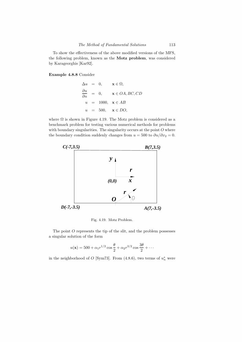
The Method of Fundamental Solutions 113
To show the effectiveness of the above modified versions of the MFS,
the following problem, known as the Motz problem, was considered
by Karageorghis [Kar92].
Example 4.8.8 Consider
∆u = 0, x ∈ Ω,
∂u
∂n= 0, x ∈ OA,BC,CD
u = 1000, x ∈ AB
u = 500, x ∈ DO,
where Ω is shown in Figure 4.19. The Motz problem is considered as a
benchmark problem for testing various numerical methods for problems
with boundary singularities. The singularity occurs at the point O where
the boundary condition suddenly changes from u = 500 to ∂u/∂x2 = 0.
A(7,-3.5)
B(7,3.5)C(-7,3.5)
D(-7,-3.5)
(0,0) x
y
rO
r
Fig. 4.19. Motz Problem.
The point O represents the tip of the slit, and the problem possesses
a singular solution of the form
u(x) = 500 + α1r1/2 cos
θ
2+ α2r
3/2 cos3θ
2+ · · ·
in the neighborhood of O [Sym73]. From (4.8.6), two terms of usn were

114
chosen. The solution is approximated by
un(x) = α1r1/2 cos
θ
2+ α2r
3/2 cos3θ
2+
n∑
j=1
ajG(x,yj), yj ∈ Γ.
By taking derivatives with respect to x and y, we obtain
∂
∂xr
12 cos
θ
2=
1
2r
−12 cos
θ
2,
∂
∂yr
12 cos
θ
2=
1
2r
−12 sin
θ
2
∂
∂xr
32 cos
θ
2=
3
2r
12 cos
θ
2,
∂
∂yr
32 cos
θ
2= −3
2r
12 sin
θ
2.
The boundary conditions become
∂un
∂n= 0, x ∈ OA,
un + α1r12 cos
θ
2+ α2r
32 cos
3θ
2− 1000 = 0, x ∈ AB,
∂un
∂n+α1
2r
−12 sin
θ
2− 3α2
2r
12 sin
θ
2= 0, x ∈ BC,
∂un
∂n− α1
2r
−12 cos
θ
2− 3α2
2r
12 cos
θ
2= 0, x ∈ CD,
un − 500 = 0, x ∈ DO.
The problem was tackled by the following four different methods [PKG98]:
MFS1 Naive MFS.
MFS2 Modified MFS with α1 as only additional unknown.
MFS3 Modified MFS with α and β in (4.8.7) as additional unknowns.
MFS4 Modified MFS with α1 and α2 as unknowns [Kar92].
The sources were initially placed outside the domain at different dis-
tances d from the boundary, as before. Due to the strong nonlinearity
of the resulting problem in the new modified method, convergence was
achieved only for a restricted range of d less than 0.4. The exact so-
lution [RP75] and approximate solutions using the MFS1 – MFS4 with
n = 66,m = 7, and a maximum of 4000 function evaluations are shown
in Table 4.16. The numerical results reveal that MFS4 is the most ac-
curate.
The calculated values of α1 and β1 are given in Table 4.17 for various
values of the initial distance of the moving sources from the boundary.
These are in excellent agreement with the exact values α1 = 151.63, β1 =
0.5.
2

The Method of Fundamental Solutions 115
(x, y) MFS1 MFS2 MFS3 MFS4 Exact
(−0.5,−3.0) 578.95 547.59 546.04 546.31 546.24
(−0.25,−3.0) 605.05 559.30 557.32 557.72 557.64
(0.0,−3.0) 631.08 576.48 574.20 574.70 574.61
(0.25,−3.0) 655.27 598.17 595.82 596.31 596.23
(0.5,−3.0) 677.50 620.75 618.49 618.92 618.85
(−0.5,−3.25) 553.03 526.03 524.63 524.89 524.81
(−0.25,−3.25) 590.52 535.61 533.17 533.71 533.59
(0.0,−3.25) 622.50 555.54 552.54 553.30 553.19
(0.25,−3.25) 649.86 586.07 583.12 583.76 583.67
(0.5,−3.5) 673.90 614.14 611.44 611.93 611.86
(−0.5,−3.5) 530.90 501.69 499.97 500.11 500.00
(−0.25,−3.5) 582.26 502.50 499.63 500.18 500.00
(0.0,−3.5) 618.48 503.46 496.80 500.26 500.00
(0.25,−3.5) 647.70 579.39 575.80 576.48 576.41
(0.5,−3.5) 672.73 611.66 608.48 608.96 608.91
Table 4.16. Approximate solution near the singularity O.
4.8.3 Axisymmetric Potential Problems
When working on an axisymmetric three-dimensional domain Ω, the
potential equation using the Laplace operator can be rewritten as
∆u =∂2u
∂r2+
1
r
∂u
∂r+∂2u
∂z2= 0, x ∈ Ω, (4.8.9)
where z is the coordinate along the axis and r is the distance to the axis.
If the boundary conditions are also axisymmetric, a 3D problem can be
reduced to a 2D problem in the variables r and z.
Karageorghis and Fairweather [KF99] considered the following axi-
symmetric mixed potential problem
∆u = 0, x ∈ Ω,
Bu = 0, x ∈ Γ,(4.8.10)

116
m n d NFEV α1 β1
7 66 0.4 2500 149.72 0.453000 150.85 0.443500 150.88 0.444000 150.88 0.44
7 66 0.6 2500 150.14 0.473000 150.14 0.473500 150.14 0.474000 150.14 0.47
10 96 0.5 2500 150.92 0.473000 150.51 0.473500 150.43 0.474000 150.39 0.47
10 96 0.6 2500 149.77 0.483000 149.17 0.483500 149.13 0.484000 149.13 0.48
Table 4.17. Approximate value of α1 and β1.
on an axisymmetric domain Ω ⊂ IR3 with boundary Γ. The boundary
operator B has the form
Bu =
α(x) + u(x), x ∈ ΓD1 , (Dirichlet part)
α(x) +∂u
∂n(x), x ∈ ΓN
2 , (Neumann part)
α(x) + β(x)u(x) + γ(x)∂u
∂n(x), x ∈ ΓR
3 , (Robin part)
where α, β, and γ are prescribed axisymmetric functions.
4.8.4 Axisymmetric boundary conditions
Since the boundary conditions are assumed to be axisymmetric, the 3D
problem in (4.8.10) reduces to a 2D problem via (4.8.9). Let p = (rp, zp)
and q = (rq, zq) be two points in Ω in axisymmetric coordinates (r, z)
and define
ρ(p,q) =√
(rp − rq)2 + (zp − zq)2 (4.8.11)

The Method of Fundamental Solutions 117
to be their standard Euclidean distance in these coordinates. Then the
fundamental solution of equation (4.8.9) is given by
G(p,q) =4K(κ(p,q))
ρ(p,q)(4.8.12)
where
K(κ) =
∫ 2π
0
1√1 − κ2 sin2(θ)
dθ and κ2(p,q) =4rprqρ2(p,q)
.
(4.8.13)
is the complete elliptic integral of the first kind. Furthermore, since
∂G(p,q)
∂n=∂G(p,q)
∂rnr +
∂G(p,q)
∂znz
where ∂/∂n denotes the outward normal derivative at the boundary
point q, and nr and nz are the components of the outward unit vector
to Γ in the r and z direction, respectively, one obtains
∂G(p,q)
∂n
=2ρ3/2
[E(κ) −K(κ)(1 − κ2)] − 2rq(rq + rp)E(κ)
]
rqρ3/2(1 − κ)2nr
−4(zq − zp)E(κ)
ρ3/2(1 − κ2)nz
where E(κ) is the complete elliptic integral of the second kind defined
by
E(κ) =
∫ 2π
0
√1 − κ2 sin2(θ)dθ,
and where the dependence of ρ and κ on p and q is dropped to simplify
the notation. OnceG(p,q) and ∂G(p,q)/∂n are available, the numerical
approximation un of the true solution can be represented by (4.2.8).
Note that in the case of simple connected domains, no boundary points
are placed on the axis of rotation.
The complete elliptic integrals K(κ) and E(κ) are evaluated using
the NAG routines S21BBF and S21BCF, or the IMSL routines ELK
and ELE, respectively.
Example 4.8.14 The problem of steady-state heat conduction through
a hollow cylinder with insulated ends is investigated [KF99] using the

118
‖u− un‖∞NFEV m = 32, n = 4 m = 64, n = 8 m = 128, n = 16
500 7.0E−3 1.5E−3 3.8E−41000 6.9E−3 5.9E−4 1.9E−52000 4.2E−3 3.6E−4 9.9E−63000 3.1E−3 2.3E−5 8.1E−64000 3.0E−3 2.0E−5 5.6E−65000 3.0E−3 1.7E−5 3.7E−6
Table 4.18. Results for the temperature distribution.
MFS. The inner and outer radii of the cylinder are denoted by ri and
ro, respectively. The boundary conditions are prescribed as
u = f, for r = ri,
u = g, for r = ro,∂u
∂z= 0, for z = ±z0.
The analytical solution [Cha67] is
u = f + (g − f)ln(r/ri)
ln(ro/ri).
The following parameter values were chosen:
ri = 1, ro = 2, z0 = 0.5, f = 1, g = 2.
The numerical computations were performed on a 0.1 × 0.1 grid for
various values of
NFEV = number of function evaluations
m = number of collocation points
n = number of source points
The errors ‖u− un‖∞ and ‖∂u/∂r− ∂un/∂r‖∞ are shown in Table 4.18
and 4.19.
2

The Method of Fundamental Solutions 119
‖∂u/∂r − ∂un/∂r‖∞NFEV m = 32, n = 4 m = 64, n = 8 m = 128, n = 16
500 4.0E−2 1.5E−2 3.8E−31000 6.9E−2 5.9E−3 1.9E−42000 4.2E−2 3.6E−3 9.9E−43000 3.1E−2 2.3E−4 8.1E−54000 3.0E−2 2.0E−4 5.6E−55000 3.0E−2 1.7E−4 3.7E−5
Table 4.19. Results for the flux.
4.8.5 Non–axisymmetric boundary conditions
For non–axisymmetric boundary conditions, the solution u is expanded
in Fourier series as
u(p) =u0(rp, zp)
2+
∞∑
i=1
[uci(rp, zp) cos(iθp) + us
i (rp, zp) sin(iθp)]
(4.8.15)
where p = (rp, zp), and where the functions uci and us
i satisfy a differ-
ential equation of the form
∂2u(p)
∂r2+
1
r
∂u(p)
∂r+∂2u(p)
∂z2−(i
r
)2
u = 0, p ∈ Ω, for i = 0, 1, 2, · · · .(4.8.16)
The fundamental solutions of (4.8.16) can be written in terms of com-
plete elliptic integrals [Gup79] as
Gi =4Ki(κ)
ρ, i ≥ 0
as in (4.8.12) and (4.8.13), with
K0(κ) = K(κ),
Ki(κ) = (−1)ii
m∑
j=0
Lij2
2(i−j)Ci−j , i ≥ 1,
Lij = (−1)j (2i− j − 1)!
j!(2i− 2j)!, j = 0, 1, · · · , i,

120
C0 := K(κ),
C1 :=1
κ2
(E(κ) − (1 − κ2)K(κ)
)
Cn :=(2n− 2)
(2κ2 − 1
)Cn−1 + (2n− 3)
(1 − κ2
)Cn−2
(2n− 1)κ2, n ≥ 2.
The normal derivatives of the fundamental solutions are [Gup79]
∂Gi(p,q)
∂n
=4
ρ2
[(ρ∂Ki
∂κ
∂κ
∂rq−Ki
∂ρ
∂r′
)nr +
(ρ∂Km
∂κ
∂κ
∂zq−Ki
∂ρ
∂zq
)nz
],
where
∂ρ
∂rq=
rq + rpρ
,
∂ρ
∂zq=
zq − zpρ
,
∂κ
∂rq=
2rp − κ2(rq + rp)
κρ2,
∂κ
∂zq=
κ (zq − zp)
ρ2.
Furthermore,
∂K0(k)
∂k=
∂K(k)
∂k
∂Ki(k)
∂k= (−1)ii
i∑
j=0
Lmj 22(m−j) ∂Ci−j
∂k, i ≥ 1,
∂Cℓ
∂κ=
E(κ) − (1 − κ2)K(κ)
κ(1 − κ2), ℓ = 0,
(2 − κ2)K(κ) − 2E(κ)
κ3, ℓ = 1,
2ℓ− 2
(2ℓ− 1)κ2
[(2κ2 − 1
) ∂Cℓ−1
∂κ+
2
κCℓ−1
]
+2ℓ− 3
(2ℓ− 1)κ2
[(1 − κ2
) ∂Cℓ−2
∂κ− 2
κCℓ−2
],
ℓ ≥ 2.

The Method of Fundamental Solutions 121
Example 4.8.17 Here, the problem of uniaxial flow in a finite cylindri-
cal region of an infinite medium is considered. The direction of heat flow
in this case is not along the axis of the cylindrical region, thus resulting
in non–axisymmetric boundary conditions. Let the boundary conditions
be as follows [Gup79]:
u = 2r cos θ on z = 0,
u = 2r cos θ on z = 2,
u = 2 cos θ on r = 2.
The exact solution of the problem is given by u = 2r cos θ. Note that
the only non–zero Fourier coefficient is uc1 in (4.8.15); i.e. i = 1. The
errors e = ‖u− um‖∞ and er = ‖∂u/∂r − ∂um/∂r‖∞ are computed on
a grid of cell width 0.2 and the results [KF99] are shown in Table 4.20.
2
n = 3,m = 24 n = 6, m = 48 n = 12, m = 96NFEV e er e er e er
500 2.1E−5 5.1E−5 9.6E−5 5.4E−4 2.9E−3 3.9E−31000 1.5E−5 3.8E−5 2.2E−5 1.9E−4 2.2E−4 7.4E−42000 1.0E−5 2.5E−5 8.7E−6 4.7E−5 1.3E−5 3.8E−53000 7.6E−6 1.8E−5 4.2E−6 2.2E−5 4.2E−6 2.9E−54000 5.6E−6 1.3E−5 2.1E−6 1.4E−5 3.2E−6 1.9E−55000 4.3E−4 1.0E−5 1.5E−6 9.4E−6 1.5E−6 8.4E−6
Table 4.20. Errors of e = ‖u− um‖∞ and er = ‖∂u/∂r − ∂um/∂r‖∞
4.8.6 Acoustic Scattering and Radiation Problems
Such problems are governed by the Helmholtz equation
(∆ + λ2)u(p) = 0, p ∈ Ω,
Bu(p) = f(p), p ∈ Γ,
where B is a boundary operator and λ the wave number. Let p =
(rp, zp, θp),q = (rq, zq, θq). Define
ρ (p,q) =√r2p + r2q − 2rprq cos(θq − θp) + (zq − zp)2.

122
The fundamental solution of the axisymmetric version of the Helmholtz
equation is given by
G(p,q) =
∫ 2π
0
e−iλρ(p,q)
ρ (p,q)dθ(q).
G(p,q) can be written into two parts, consisting of a nonsingular and a
singular integral
G(p,q) =
∫ 2π
0
e−iλρ(p,q) − 1
ρ (p,q)dθ(q) +
∫ 2π
0
1
ρ (p,q)dθ(q)
= G1(p,q) +G2(p,q).
Notice that G1 can be evaluated using a standard quadrature rule. As
shown in the previous example, we have
G2(p,q) =4K(κ)
ρ
where K(κ) and ρ are given in (4.8.11) and (4.8.13), and the normal
derivative of G(p,q) can be written in terms of K(κ) and E(κ). The
formulation of the MFS is similar to the bi-harmonic equation described
in Section 4.6. As a result, there are 4M unknowns to be determined
using dynamic approach. For the acoustic radiation and scattering prob-
lems for axisymmetric bodies in the half space z > 0, the problem of
discretizing the plane z = 0 is avoided by using an appropriate fun-
damental solution. When the plane is rigid, the following fundamental
solution is available:
GH(p,q) =
∫ 2π
0
e−iλρ(p,q) − 1
ρ (p,q)dθ(q) +
∫ 2π
0
e−iλρ(p′,q) − 1
ρ (p′,q)dθ(q)
where the point p′ is the image point of p in the plane. This fundamental
solution satisfies the axisymmetric version of the Helmholtz equation and
the boundary condition for a rigid plane, ∂u/∂z = 0 on z = 0.
For numerical examples, we refer the reader to [KF98].
4.8.7 Nonlinear Boundary Conditions
One of the criticisms of the MFS, when the dynamic approach is used,
is that linear problems are solved by means of a nonlinear technique. In
this subsection, we present problems which are governed by Laplace’s
equation and are subject to nonlinear boundary conditions [KF89a].

The Method of Fundamental Solutions 123
The mathematical formulation of the MFS does not depend on the lin-
earity of the boundary conditions, as we shall see, and it can be easily
adapted to such problems.
Consider the following Laplace equation subject to the nonlinear bound-
ary condition
∆u = 0, x ∈ Ω,
Bu = 0, x ∈ Γ,
where B is a nonlinear operator. Similar to the problems with linear
boundary conditions, the approximate solution un can be represented
by a linear combination of fundamental solutions as shown in (4.2.8). In
particular, Karageorghis and Fairweather [KF89a] considered operators
of the form
Bu(x) = α(x)u(x) + β(x)∂u
∂n(x) + γ(x)u(x)4 + δ(x), x ∈ Γ.
The least squares subroutines outlined in Section 4.6 can be used to
minimize the sum of squares
εm =
m∑
i=1
|fi|2
where
fi = α(xi)
n∑
k=1
akG(xi,yk) + β(xi)
n∑
k=1
ak∂
∂nG(xi,yk)
+γ(xi)
(n∑
k=1
akG(xi,yk)
)4
+ δ(xi), 1 ≤ i ≤ m.
The initial location of source points and the initial values of ak are taken
to be the same as in the linear cases mentioned in the previous sections.
Example 4.8.18 Consider the following nonlinear boundary problem
∆u = 0, x ∈ Ω,
∂u
∂n= u(x) + u4(x), x ∈ AB,
∂u
∂n= −u(x) − u4(x), x ∈ BC,
∂u
∂n= 0, x ∈ CD,
u = 1, x ∈ DA,

124
where Ω = x = (x1, x2) : 0 ≤ x1 ≤ 1, 0 ≤ x2 ≤ 0.1. The problem do-
main Ω is shown in Figure 4.20. This problem arises in the study of
heat transfer from finned surfaces (Kern and Kraus [KK72]), which was
solved using a boundary element approach by Ingham et. al. [IHM81].
The problem was also solved by Karageorghis and Fairweather [KF89a]
using the MFS, and their results were in good agreement with those
obtained by Ingham et. al. [IHM81]. In addition to the difficulties
of nonlinear boundary conditions, the large aspect ratio of the region
(AB = 1, BC = 0.1) causes further complications.
The numerical results at some selected points obtained by Karageorghis
and Fairweather [KF89a] using the dynamic approach are shown in Table
4.21. Variousm,n and maximal numbersNFEV of function evaluations
were used in their tests. Table 4.21. uses the following notations:
MFS1: m = 13, n = 120, NFEV = 1500
MFS2: m = 13, n = 120, NFEV = 2000
BEM: Ingham et. al. [IHM81]
(x1, x2) MFS1 MFS2 BEM
(0.2, 0.02) 0.5091 0.5110 0.5073
(0.4, 0.02) 0.2714 0.2745 0.2734
(0.6, 0.02) 0.1494 0.1510 0.1510
(0.2, 0.04) 0.5171 0.5192 0.5152
(0.4, 0.04) 0.2751 0.2783 0.2772
(0.6, 0.04) 0.1515 0.1531 0.1531
(0.2, 0.06) 0.5229 0.5250 0.5210
(0.4, 0.06) 0.2778 0.2810 0.2800
(0.6, 0.06) 0.1530 0.1546 0.1546
Table 4.21. Approximate solution of u at 9 selected points.
2
4.9 Inverse Problems
Let Ω be a simply connected domain in IRd, d = 2, 3, and Γ1, Γ2, Γ3
be three parts of the boundary Γ. Suppose that Γ1 ∪ Γ2 ∪ Γ3 = Γ,
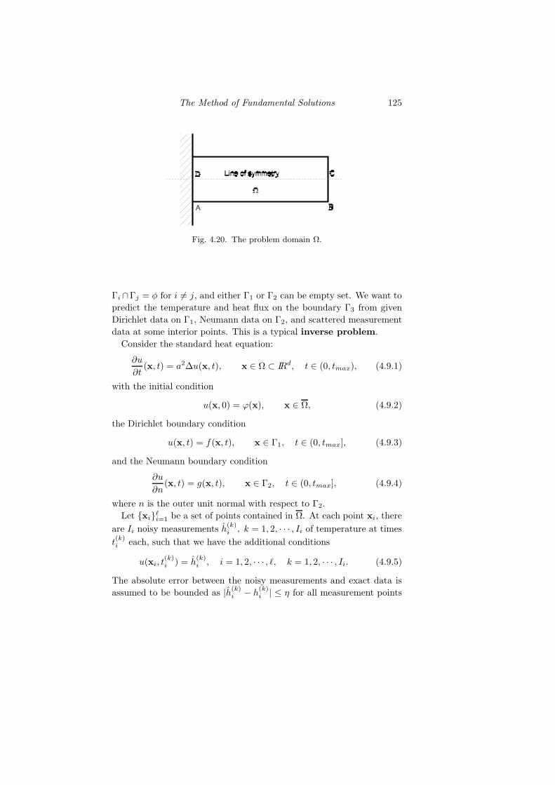
The Method of Fundamental Solutions 125
Fig. 4.20. The problem domain Ω.
Γi ∩Γj = φ for i 6= j, and either Γ1 or Γ2 can be empty set. We want to
predict the temperature and heat flux on the boundary Γ3 from given
Dirichlet data on Γ1, Neumann data on Γ2, and scattered measurement
data at some interior points. This is a typical inverse problem.
Consider the standard heat equation:
∂u
∂t(x, t) = a2∆u(x, t), x ∈ Ω ⊂ IRd, t ∈ (0, tmax), (4.9.1)
with the initial condition
u(x, 0) = ϕ(x), x ∈ Ω, (4.9.2)
the Dirichlet boundary condition
u(x, t) = f(x, t), x ∈ Γ1, t ∈ (0, tmax], (4.9.3)
and the Neumann boundary condition
∂u
∂n(x, t) = g(x, t), x ∈ Γ2, t ∈ (0, tmax], (4.9.4)
where n is the outer unit normal with respect to Γ2.
Let xiℓi=1 be a set of points contained in Ω. At each point xi, there
are Ii noisy measurements h(k)i , k = 1, 2, · · · , Ii of temperature at times
t(k)i each, such that we have the additional conditions
u(xi, t(k)i ) = h
(k)i , i = 1, 2, · · · , ℓ, k = 1, 2, · · · , Ii. (4.9.5)
The absolute error between the noisy measurements and exact data is
assumed to be bounded as |h(k)i − h
(k)i | ≤ η for all measurement points

126
at all measured times. Here, the constant η is called the noise level of
the input data.
Our goal is to reconstruct the temperature u and the heat flux ∂u/∂n
on the boundary Γ3 from the given conditions in (4.9.1)–(4.9.4) and the
scattered noisy measurements (4.9.5).
It is well known that the fundamental solution of the heat equation
(4.9.1) is given by
G(x,y, t) =1
(4πa2t)d/2exp
(− r2
4a2t
)H(t),
where r = ‖x− y‖ and H(t) is the Heaviside function. Assuming that
T > tmax is a constant, the function
φ(x, t) := G(x, t+ T ) (4.9.6)
is a solution of (4.9.1) in the solution domain Ω × [0, tmax].
We rearrange the measurement points to be (xj , tj), j = 1, · · · ,m =∑ℓi=1 Ii. Note that two measurements taken at the same location xi
but at different times are now treated as two distinct collocation points.
The collocation points are renumbered as
(xj , tj), j = m+ 1, · · · ,m+ n on Ω × 0,
(xj , tj), j = m+ n+ 1, · · · ,m+ n+ p on Γ1 × (0, tmax],
(xj , tj), j = m+ n+ p+ 1, · · · ,m+ n+ p+ q on Γ2 × (0, tmax].
Here, n, p, q denote the total number of collocation points for the initial
condition (4.9.2), Dirichlet boundary condition (4.9.3), and Neumann
boundary condition (4.9.4), respectively. In this way, we treat time as
an additional spatial dimension. As a result, the collocation points are
now distributed in a (d+ 1)-dimensional space-time.
Using the MFS, an approximation u to the solution of (4.9.1) under
the conditions (4.9.2)-(4.9.4) with the noisy measurements hj can be
expressed as follows:
u(x, t) =
n+m+p+q∑
j=1
αjφ(x − xj , t− tj),
where φ(x, t) is given by (4.9.6) and αj are unknown coefficients to be
determined.
In this way, the procedure for solving homogeneous time–dependent
problems is the same as for solving elliptic problems. Since φ is the

The Method of Fundamental Solutions 127
fundamental solution of the heat equation, the approximate solution
u automatically satisfies the original heat equation (4.9.1) inside the
domain. We need only to fit the boundary conditions. Using the initial
condition (4.9.2) and collocating the boundary conditions (4.9.3) and
(4.9.4), we then obtain the following system of linear equations:
Gα = b, (4.9.7)
where
G =
φ(xi − xj , ti − tj) 1 ≤ i ≤ m
φ(xi − xj , ti − tj) m+ 1 ≤ i ≤ m+ n
φ(xi − xj , ti − tj) m+ n+ 1 ≤ i ≤ m+ n+ p
∂u∂n (xk − xj , tk − tj) m+ n+ p+ 1 ≤ i ≤ m+ n+ p+ q
where the column index j always runs from 1 to m+n+ p+ q to match
the vector
α =(α1, α2, . . . , αn+m+p+q)T
and where
b =
hi 1 ≤ i ≤ m
ϕ(xi, ti) m+ 1 ≤ i ≤ m+ n
f(xi, ti) m+ n+ 1 ≤ i ≤ m+ n+ p
g(xi, ti) m+ n+ p+ 1 ≤ i ≤ m+ n+ p+ q
.
Note that this method, in contrast to many standard methods for inverse
problems, does not need a separate solver for the direct problem. It
solves both the direct and the inverse problem simultaneously, but it is
not recommended for solving the direct problem alone.
The solvability of the system (4.9.7) depends on the non–singularity of
the matrix G, which is still an open research problem. Due to the large
number of collocation points, the resultant matrix G is very large, and
in addition it is extremely ill–conditioned and thus ill-posed, if the trial
centers get dense. To alleviate the extreme ill–conditioning for the in-
verse problem indicated above, a regularization technique is needed. As
we note in Section 2.5, regularization can produce a stable and accurate
solution for the unknown parameters α of the matrix equation (4.9.7).
The singular value decomposition (SVD) usually works well for the di-
rect problem [Ram02] but fails to provide a stable and accurate solution
to the system (4.9.7) for the inverse problem. A number of regulariza-
tion methods have been applied to solving this kind of ill–conditioning

128
problem, and in Section 2.5 we described Tikhonov regularization,
the truncated singular value decomposition, and the L–curve
method.
After solving (4.9.7) by regularization with a parameter δ along the
lines mentioned in Section 2.5, the corresponding approximate solution
for the problem (4.9.1)–(4.9.4) with noisy measurement data is then
given by
uδ(x, t) :=
N∑
j=1
αδjφ(x − xj , t− tj)
for N = m + n + p + q. The temperature and heat flux at the surface
Γ3 can also be calculated accordingly.
Example 4.9.8 Let the heat conduction coefficient a = 1 and tmax = 1
in (4.9.1). The noisy data are generated by hi = hi + η r(i), where hi
is the exact data and r(i) is a random number in [−1, 1]. The scalar η
indicates the noise level of the measurement data.
To validate the accuracy of the approximate solution, we compute the
Root Mean Square Error (RMSE) which is defined by
E(u) =
√√√√ 1
Nt
Nt∑
i=1
(uδ(zi, τi) − u(zi, τi)) 2,
with a total of Nt evaluation points (zi, τi) in the domain Γ3 × [0, 1]
where uδ(zi, τi) and u(zi, τi) are the approximate and exact temperature
respectively at a test point. The error E(∂u/∂n) for the heat flux is
defined in a similar way.
The boundary conditions f(x, t), g(x, t) and the initial temperature
ϕ(x, t) are chosen in such a way that they satisfy the exact solution
u∗(x1, x2, t) = 2t+1
2(x2
1 + x22) + e−t(cos(x1) + cos(x2))
of (4.9.1).
Three different domain and boundary configurations are considered:
Case 1:
Ω = (x1, x2) | 0 < x1 < 1, 0 < x2 < 1,Γ1 = (x1, x2) | x1 = 1, 0 < x2 < 1,Γ2 = (x1, x2) | 0 < x1 < 1, x2 = 1,Γ3 = ∂Ω \ Γ1 ∪ Γ2.

The Method of Fundamental Solutions 129
0 0.2 0.4 0.6 0.8 10
0.1
0.2
0.3
0.4
0.5
0.6
0.7
0.8
0.9
1
x1
x 2
Ω
Γ2
Γ1
Γ3
Γ3
Case 1.
Fig. 4.21. The distribution of measurement and collocation points for the Case1.
Case 2:
Ω = (x1, x2) | x21 + x2
2 < 1,Γ1 = ∅,Γ2 = (x1, x2) | x2
1 + x22 = 1, x1 > 0,
Γ3 = ∂Ω \ Γ1 ∪ Γ2.
Case 3: Ω as in Case 1, Γ1 = Γ2 = ∅, Γ3 = ∂Ω \ Γ1 ∪ Γ2.
The distributions of the internal measurements and collocation points
over Ω for the three cases are shown in Figures 4.21-4.23. In these
figures,
* represents a collocation point for Dirichlet data,
2 represents a collocation point for Neumann data,
· represents a collocation point for initial data, and
represents points with a sensor for internal measurement.
Numerical results are obtained by taking the constant T = 1.8 in all
three cases. In Case 1,
n = 36, m = 100, p = 55, q = 50.
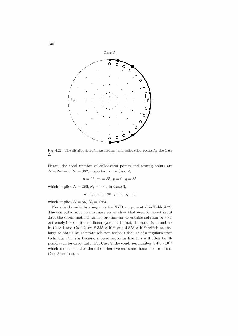
130
Ω Γ3
Γ2
Case 2.
Fig. 4.22. The distribution of measurement and collocation points for the Case2.
Hence, the total number of collocation points and testing points are
N = 241 and Nt = 882, respectively. In Case 2,
n = 96, m = 85, p = 0, q = 85.
which implies N = 266, Nt = 693. In Case 3,
n = 36, m = 30, p = 0, q = 0,
which implies N = 66, Nt = 1764.
Numerical results by using only the SVD are presented in Table 4.22.
The computed root mean-square errors show that even for exact input
data the direct method cannot produce an acceptable solution to such
extremely ill–conditioned linear systems. In fact, the condition numbers
in Case 1 and Case 2 are 8.355 × 1033 and 4.878 × 1034 which are too
large to obtain an accurate solution without the use of a regularization
technique. This is because inverse problems like this will often be ill-
posed even for exact data. For Case 3, the condition number is 4.5×10¹⁹
which is much smaller than the other two cases and hence the results in
Case 3 are better.

The Method of Fundamental Solutions 131
0 0.2 0.4 0.6 0.8 10
0.1
0.2
0.3
0.4
0.5
0.6
0.7
0.8
0.9
1 Case 3.
Ω
Γ3
Γ3 Γ
3
Γ3
Fig. 4.23. The distribution of measurement and collocation points for the Case3.
The use of regularization techniques, as we shall see, gives a stable and
much more accurate solution. Table 4.23 shows the root mean-square
errors of the temperature and heat flux in domain Γ3 × [0, 1] with exact
data, using Tikhonov regularization with an L-curve-based choice of the
regularization parameter δ. In contrast to Table 4.22, the RMSE errors
in Table 4.23 are greatly reduced. We remark that the L-curve method
works well for determining the crucial regularization parameter, but it
can be further improved if a scaling factor is used.
Numerical results for the example with noisy data (noise level η = 0.01
in all cases) are shown in Table 4.24. The regularization method with the
L-curve technique provides an acceptable approximation to the solution
whilst the direct method fails completely. The problem of how to choose
an optimal regularization parameter is still an open question.
Note that the setting for Case 3 comes from a real-life problem in a
steel company. In fact, the solution for this case may not be unique,
but our computational results demonstrate that the proposed method is
flexible enough to give a reasonable approximation to the solution under
insufficient information.

132
Case 1E(u)= 11.2115
E(∂u/∂n) = 4.6189
Case 2E(u) = 12.2759
E(∂u/∂n) = 2.1023
Case 3E(u) = 0.0104
E(∂u/∂n) = 0.0556
Table 4.22. RMSE in domain Γ3 × [0, 1] with exact data and no
regularization technique.
Case 1δ = 2.7404E − 12 E(u)= 2.7289E − 04
E(∂u/∂n) = 6.7662E − 04
Case 2δ = 4.1551E − 13 E(u) = 0.0011
E(∂u/∂n)= 0.0029
Case 3δ = 1.0370E − 8 E(u) = 0.0013
E(∂u/∂n) = 0.0062
Table 4.23. RMSE in domain Γ3 × [0, 1] with exact data by using
Tikhonov regularization with L-curve parameter δ.
The relationship between the RMSE and the value of the constant
T in Case 1 with noisy data (η = 0.01) is displayed in Figure 4.24.
The regularization parameter δ is obtained again by using the L-curve
method. The numerical results indicate that the choice of the parameter
T plays an important role for obtaining an accurate approximation.
2
Example 4.9.9 Let
Ω = (x1, x2, x3) : 0 < xi < 1, i = 1, 2, 3Γ1 = (x1, x2, x3) : 0 < x1 < 1, 0 < x2 < 1, x3 = 1Γ2 = (x1, x2, x3) : 0 < x1 < 1, 0 < x2 < 1, x3 = 0Γ3 = ∂Ω \ (Γ1 ∪ Γ2).
The locations of the measurement points and the collocation points in
the domain Ω are shown in Figure 4.25 where
∗ represents a measurement point with Dirichlet data,

The Method of Fundamental Solutions 133
Case 1δ = 6.9833E − 5 E(u)= 0.0266
E(∂u/∂n) = 0.0538
Case 2δ = 0.003 E(u)= 0.2456
E(∂u/∂n) = 0.4211
Case 3δ = 6.7772E − 7 E(u)= 0.0290
E(∂u/∂n) = 0.0608
Table 4.24. RMSE in domain Γ3 × [0, 1] with noisy data (η = 0.01) by
Tikhonov regularization with L-curve parameter δ
1 2 3 4 5 6 7 8 9 100
0.01
0.02
0.03
0.04
0.05
0.06
parameter T
RM
S(u
) and
RM
S(d
u)
For case 1. σ=0.01
Fig. 4.24. RMSE of temperature and heat flux on Γ3 × [0, 1] with respect tothe parameter T.
2 represents a measurement point with Neumann data, and
represents a point with sensor data.
In this computation, we set
n = 245, m = 250, p = 180, q = 180, N = 855, Nt = 5324.

134
0
0.5
1
0
0.5
10
0.2
0.4
0.6
0.8
1
x1
x2
x 3
Γ1
Γ2
Ω
Fig. 4.25. Locations of measurement and collocation points.
00.5
1
0
0.5
1−5
0
5
x 10−3
x1
x3
Err
or o
f u(x
1,0,x
3,1)
00.5
1
0
0.5
1−2
0
2
4
x 10−3
x2
x3
Err
or o
f u(0
,x2,x
3,1)
00.5
1
0
0.5
1−5
0
5
x 10−3
x1
x3
Err
or o
f u(x
1,1,x
3,1)
00.5
1
0
0.5
1−4
−2
0
x 10−3
x2
x3
Err
or o
f u(1
,x2,x
3,1)
Fig. 4.26. Surface plots of temperature errors on boundary Γ3
The exact solution is given by
u∗(x1, x2, x3, t) = e(−4t)(cos(2x1) + cos(2x2) + cos(2x3)).
In the computation, the value of the parameter T is 2.3 and the noise
level is set to be η = 0.01. The errors between the exact solution and
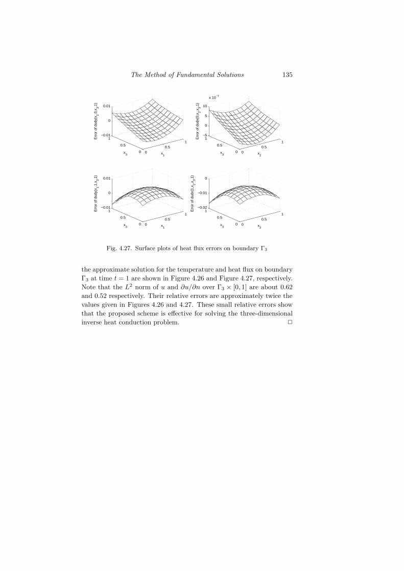
The Method of Fundamental Solutions 135
00.5
1
0
0.5
1−0.01
0
0.01
x1
x3
Err
or o
f dud
y(x 1,0
,x3,1
)
00.5
1
0
0.5
1−5
0
5
10
x 10−3
x2
x3
Err
or o
f dud
x(0,
x 2,x3,1
)
00.5
1
0
0.5
1−0.01
0
0.01
x1
x3
Err
or o
f dud
y(x 1,1
,x3,1
)
00.5
1
0
0.5
1−0.02
−0.01
0
x2
x3
Err
or o
f dud
x(1,
x 2,x3,1
)
Fig. 4.27. Surface plots of heat flux errors on boundary Γ3
the approximate solution for the temperature and heat flux on boundary
Γ3 at time t = 1 are shown in Figure 4.26 and Figure 4.27, respectively.
Note that the L2 norm of u and ∂u/∂n over Γ3 × [0, 1] are about 0.62
and 0.52 respectively. Their relative errors are approximately twice the
values given in Figures 4.26 and 4.27. These small relative errors show
that the proposed scheme is effective for solving the three-dimensional
inverse heat conduction problem. 2
5
The Method of Particular Solutions
5.1 Introduction
In the last chapter, we considered only linear homogeneous equations
having fundamental solutions. In this chapter we extend our discussion
to linear inhomogeneous problems
Lu = fΩ in Ω ⊂ IRd
u = fD in ΓD ⊆ Γ := ∂Ω∂u
∂n= fN in ΓN ⊂ Γ = ΓD ∪ ΓN , ΓD ∩ ΓN = ∅
(5.1.1)
with Dirichlet boundary conditions on ΓD and Neumann boundary con-
ditions on ΓN . Here, fΩ, fD, fN are given functions on Ω, ΓD, ΓN ,
respectively. We shall later replace the right-hand side fΩ : Ω → IR by
fΩ(x, u,∇u, ...) to treat more general quasi-linear or nonlinear problems.
In the Boundary Element Method, it is well-known that (5.1.1)
can be reformulated as an integral equation [PBW92]
c(x)u(x) =
∫
Γ
(u(y)
∂G(x, ·)∂n
(y) − ∂u
∂n(y)G(x,y)
)dy
+
∫
Ω
G(x,y)fΩ(y)dy(5.1.2)
where x ∈ Ω∪Γ and c(x) is a geometric factor depending on the location
of x, i.e.
c(x) =
1, x in the interior,
1
2, x on a smooth boundary,
θ
2π, x at a corner with angle θ,
136

The Method of Particular Solutions 137
and G(x,y) is the fundamental solution of the differential operator L.
In (5.1.2), a domain integration is required. Due to this, the Bound-
ary Element Method (BEM) loses its attractiveness of having a bound-
ary integration only. During the past two decades, considerable effort
has been devoted to the problem of either efficiently computing the do-
main integrals or transferring them to the boundary. Even though the
domain integrals usually do not introduce any new unknowns in the nu-
merical implementation, the singularity in the integrand and the possibly
irregular shape of the domain make it difficult to evaluate the integral
with efficient numerical schemes, especially in the 3D case. In fact, the
accurate evaluation of these integrals becomes the dominating computa-
tional task in the whole numerical process for solving partial differential
equations.
In this chapter we will briefly introduce a number of approaches to al-
leviate the difficulties of domain integration in irregular domains. Later,
we shall focus on how to eliminate these domain integrations by using
radial basis functions.
5.2 The Dual Reciprocity Method (DRM)
A particular solution of a boundary-value problem (5.1.1) is defined
as a function up on Ω ∪ Γ which satisfies the inhomogeneous equation
Lup = fΩ in Ω (5.2.1)
but does not necessarily satisfy the boundary conditions of (5.1.1). No-
tice that the particular solution is not unique.
Suppose a particular solution up of (5.2.1) is known. Then the integral
equation (5.1.2) can be rewritten without any domain integral. To see
this, let I(x) be the domain integral term in (5.1.2). Then
I(x) =
∫
Ω
G(x,y)fΩ(y)dy =
∫
Ω
G(x,y)Lup(y)dy. (5.2.2)
Using Green’s Theorem, we have
∫
Ω
(G(x,y)Lup(y) − up(y)LG(x,y)) dy
=
∫
Γ
(G(x,y)
∂up
∂n(y) − up(y)
∂G(x, ·)∂n
(y)
)dy,

138
and thus get
I(x) =
∫
Ω
G(x,y)Lup(y)dy
=
∫
Ω
up(y)(LG(x, ·))(y)dy
+
∫
Γ
(G(x,y)
∂up
∂n(y) − up(y)
∂G(x, ·)∂n
(y)
)dy.
(5.2.3)
We note that fundamental solutions satisfy LG(x, ·) = δx. Furthermore,
the domain integral term in the right hand side of (5.2.3) is equal to
c(x)up(x). From (5.2.2) and (5.2.3), we finally get
I(x) = c(x)up(x) +
∫
Γ
(G(x,y)
∂up
∂n(y) − up(y)
∂G(x, ·)∂n
(y)
)dy,
which contains no domain integral any more. In this way the boundary
element method can keep its advantage of having boundary integrations
only.
The above procedure to transfer the domain integral to the boundary
can be successful only if an explicit particular solution up is available.
However, the task of deriving an explicit particular solution is nontrivial
and often impossible when fΩ becomes complicated. In Section 5.5, we
will introduce a numerical scheme to approximate the particular solu-
tion. Coupling Boundary Element Methods with such a scheme is known
as the Dual Reciprocity Method (DRM). We refer the readers to the
book [PBW92] for further details on the DRM.
5.3 The Method of Particular Solutions (MPS)
Another approach for solving the inhomogeneous problem (5.1.1) is to
split the solution u into a particular solution up and its associated ho-
mogeneous solution uh as
u = uh + up. (5.3.1)
From (5.1.1) and (5.2.1) we get
Luh = Lu− Lup = fΩ − fΩ = 0.
Thus we have the homogeneous problem
Luh = 0 in Ω
uh = fD − up in ΓD
∂uh
∂n= fN − ∂up
∂nin ΓN .
(5.3.2)

The Method of Particular Solutions 139
Once up is known, the influence of the solution by the inhomogeneous
term has in fact been transferred to the boundary and the homoge-
neous solution uh in (5.3.2) can be calculated by standard boundary
methods such as the Boundary Element Method, the Method of
Fundamental Solutions, the Boundary Integral Method, etc. For
simplicity and the advantages we have discussed in the previous chapter,
the Method of Fundamental Solutions will be employed throughout
this chapter to find the homogeneous solution uh. The final solution u
can be recovered by adding uh and up as in (5.3.1). The key step of
the Method of Particular Solutions is to obtain an explicit partic-
ular solution or, at least, a good explicit approximation to it. In the
next section we will focus on the general idea of the approximation of
particular solutions via radial basis functions.
5.4 Approximate Particular Solutions
To construct a particular solution for the boundary-value problem (5.1.1)
approximately, one can take particular solutions of other boundary-value
problems
Luk = fk, 1 ≤ k ≤ n (5.4.1)
with the same linear differential operator, and approximate fΩ by a
superposition
fΩ ≃n∑
k=1
αkfk (5.4.2)
of the functions fk to some accuracy. Then the function
up :=
n∑
k=1
αkuk
satisfies
Lup =
n∑
k=1
αkLuk =
n∑
k=1
αkfk ≃ fΩ
and thus is an approximate particular solution for the boundary-
value problem (5.1.1). This reduces the construction of approximate
particular solutions of boundary-value problems to a standard approxi-
mation problem like those considered in Chapter 2.
Furthermore, the Method of Particular Solutions combined with the
Method of Fundamental Solutions leads to reliable results, because there

140
will be explicitly available functions up and uh such that in the situation
of (5.2.1) we have small residuals
Lup − fΩ =: rΩ small in Ω
uh − (fD − up) =: rD small in ΓD
∂uh
∂n− (fN − ∂up
∂n) =: rN small in ΓN .
If there is continuous dependence of the exact solution u on the data in
the sense that for each other approximate solution u the inequality
‖u− u‖ ≤ cΩ‖Lu− Lu‖Ω + cΓD‖u− u‖ΓD + cΓN ‖∂u∂n
− ∂u
∂n‖ΓN
holds in suitable norms, we have a final small error
‖u− up − uh‖ ≤ cΩ‖Lu− Lup − Luh‖Ω
+cΓD‖u− up − uh‖ΓD
+cΓN‖∂u∂n
− ∂up
∂n− ∂uh
∂n‖ΓN
= cΩ‖fΩ − Lup‖Ω
+cΓD‖fD − up − uh‖ΓD
+cΓN‖fN − ∂up
∂n− ∂uh
∂n‖ΓN
= cΩ‖rΩ‖Ω + cΓD‖rD‖ΓD + cΓN ‖rN‖ΓN .
This is a good theoretical a-posteriori justification for the method, but
in practice the constants cΩ, cΓD , cΓN are only rarely known explicitly.
For the particular solutions arising in (5.4.1) one can use any pair of
functions u, f with Lu = f , and each such pair can be called a par-
ticular solution for the differential operator L. A simple and easy
technique to get approximate particular solutions is to take some ar-
bitrary smooth and explicit u and to evaluate f := Lu explicitly in a
straightforward way. We shall use this direct technique below in some
cases, but it has the disadvantage that it is not always guaranteed that
the functions fk obtained this way are able to recover fΩ up to high
accuracy within a well-developed theory of multivariate approximation.
This limits the applicability of the direct technique somewhat, since we
require (5.4.2) to work properly. But in many cases one can start with
functions fk which provide useful approximations, and then one has to
solve for uk with Luk = fk. We call this the indirect technique.

The Method of Particular Solutions 141
Since Chapter 2 provides a well-established theory for approximation
by radial basis trial functions, this chapter focuses on the indirect tech-
nique to derive particular solutions u such that f = Lu is a translate
φ(‖ · −y‖2) of a radial basis function φ with respect to a trial point
y ∈ IRd. If n such trial centers yknk=1 are chosen, the inhomoge-
neous term fΩ is approximated as in (5.4.2) via a finite combination of
translates of radial basis functions as
fΩ(x) ≃ f(x) :=
n∑
k=1
αkφ(‖x − yk‖2) (5.4.3)
where αknk=1 is a vector of coefficients to be determined. If we do
the approximation in (5.4.3) by interpolation, and take the trial centers
yknk=1 also as test points, we have to satisfy the conditions
fΩ(yj) = f(yj), 1 ≤ j ≤ n,
which lead to the linear system
fΩ (yj) =
n∑
k=1
αkφ(‖yj − yk‖2), 1 ≤ j ≤ n, (5.4.4)
which is uniquely solvable if the symmetric n× n matrix
A =
φ(‖y1 − y1‖2) · · · φ(‖y1 − yn‖2)
.... . .
...
φ(‖yn − y1‖2) · · · φ(‖yn − yn‖2)
is nonsingular. If φ is a positive definite radial basis function, Definition
1.2.4 in Chapter 1 even guarantees that the matrix is positive definite
which implies that the matrix is nonsingular.
Therefore we need to find particular solutions uk such that
Luk(x) = φ(‖x − yk‖2).
If L is a radially invariant operator like the Laplace or Helmholtz oper-
ator, we get particular solutions that itself are radial basis functions
uk(x) = ψ(‖x− yk‖2).
In this case, the indirect method also works, provided that the differ-
ential operator is elliptic, e.g. for the negative Laplace operator or the
modified Helmholtz equation. Radiality will not be conserved for gen-
eral operators, but the overall logic of the Dual Reciprocity Method
stays the same. Since this book focuses on radial basis functions, we
142
shall also focus on radially invariant linear differential operators and
radial particular solutions.
Once f in (5.4.3) is established, an approximate particular solution
up to a particular solution up of (5.2.1) can be written as
up(x) =
n∑
k=1
αkψ (‖x− yk‖2) , x ∈ Ω, (5.4.5)
where ψ satisfies
Lψ(‖x − yk‖2) = φ(‖x − yk‖2), x ∈ Ω, 1 ≤ k ≤ n. (5.4.6)
The normal derivative of a particular solution (5.4.5) is
∂up
∂n(x) =
n∑
k=1
αk∂
∂nψ(‖x − yk‖2), x ∈ Ω. (5.4.7)
The above approximation of the particular solution requires knowing ψ
in (5.4.6) in closed form. Since φ is radially symmetric, the analytical
solvability of (5.4.6) for differential operators L that are radially and
translationally invariant can be expected. For these operators such as
the Laplace operator ∆ and the bi-harmonic operator ∆2, a variety of
closed-form radial particular solutions ψ are available.
Consequently, an appropriate choice of a radial basis function is of con-
siderable interest. In the past, the function φ(r) = 1+r was used almost
exclusively in the literature on Boundary Element Methods [PBW92].
Unfortunately, there is no theoretical basis to justify the ad-hoc choice
of 1 + r. However the introduction of a positive definite radial basis
functions gives a firm theoretical justification of the Dual Reciprocity
Method.
Moreover, the traditional approach of the Dual Reciprocity Method
coupled the boundary values and the domain term [PBW92] and thus
placed a substantial restriction on the choice of the interpolation points
and basis functions in (5.4.3). One of the advantages of using the Method
of Particular Solutions is that it decouples the original differential equa-
tion into two parts as shown in the previous section. Since the particular
solution is independent of the geometric shape of the solution domain,
this allows us to use a domain-embedding approach to calculate an ap-
proximate particular solution. As shown in Figure 5.1, the interpolation
points can reside inside and outside the solution domain and can be
scattered points or regular grid points in a box containing any irregular
domain Ω. The simplicity and flexibility of choosing interpolation points
in such a way are desirable when preparing the data input.

The Method of Particular Solutions 143
Fig. 5.1. Domain embedding method using scattering points (left) or irregulargrid points inside the domain (right).
In the past, due to the difficulty of obtaining closed-form particu-
lar solutions, the Dual Reciprocity Method was restricted mostly to
Poisson-type equations [PBW92]. Other types of differential equations
were treated as a generalized Poisson equation by keeping the Laplace
operator operator on the left-hand-side and moving the rest to the right
hand side, i.e.
∆u = f(x, u,∇u, ∂u∂t, ...).
The right-hand-side of the equation is treated as a known quantity by
means of iterative updating in nonlinear problems, or by time-stepping
in time–dependent problems. This is possible because RBF methods
provide smooth approximate solutions which can be evaluated or differ-
entiated everywhere.
In recent years, significant progress in deriving closed–form particu-
lar solutions for other differential operators has been reported [CR98,
MGC99]. As we shall see in the later sections, significant improvement
in efficiency and accuracy of numerical computations has been achieved
this way.

144
5.5 Particular Solutions for the Laplace operator
To obtain ψ in (5.4.6) for L = ∆, we notice that ∆ is both translationally
and rotationally invariant. In polar coordinates, we have
∆ψ =
1
r
d
dr
(rdψ
dr
), in 2D,
1
r2d
dr
(r2dψ
dr
), in 3D.
Thus one can easily determine particular solutions by the direct method,
while the indirect method requires solving a second-order ordinary dif-
ferential equation.
All cases allow a simple scaling technique. If we scale the radial basis
function φ by a positive scale factor c as φc(r) := φ(r/c) as we did in
Section 2.6 for various numerical reasons, the function
∆(c2ψ(r/c)) = φ(r/c) or ∆(c2ψc(r)) = φc(r) (5.5.1)
will solve the scaled problem. Thus we only need to focus on unscaled
particular solutions here, but note that this argument works only for
homogeneous differential operators in this straightforward way.
We first treat the direct case, which goes back to Schclar [Sch94]. It
can be proven by Fourier transform arguments that any linear elliptic
and radially symmetric operator transforms smooth positive definite ra-
dial basis functions into positive definite radial basis functions. Thus
if we start with a smooth positive definite radial basis function ψ and
take −φ := −∆ψ, the function −φ will be positive definite and radial
again, because −∆ is elliptic and radially symmetric. A more careful
analysis reveals that if ψ is a conditionally positive definite radial basis
function of positive order Q from Table 1.3, then −∆ψ will be condi-
tionally positive definite of order Q−1. This technique generates plenty
of new radial basis functions, if (−∆)m is applied to the ones we gave in
Table 1.3. Note, however, that polyharmonic splines will go into poly-
harmonic splines again. Furthermore, the procedure comes to an end
when generating singular radial basis functions after application of −∆.
In this way, it is mathematically justified to choose ψ as the particular
solution corresponding to φ := ∆ψ which is used to interpolate the
right–hand side of the given differential equation. In this way, not only
the invertibility of the interpolation matrix is guaranteed, but also the
particular solution can be obtained cheaply.

The Method of Particular Solutions 145
For the inverse multiquadric
ψ =1√
r2 + c2
the direct technique yields
φ = ∆ψ =
r2 − 2c2
(r2 + c2)5/2, in 2D,
−3c2
(r2 + c2)5/2, in 3D.
For the unscaled compactly supported Wendland–type RBF
ψ = (1 − r)6+
(35r2 + 18r + 3
), (5.5.2)
the new interpolation function is given by
φ = ∆ψ =
112 (1 − r)
4+
(20r2 − 4r − 1
), in 2D,
168 (1 − r)4+
(15r2 − 4r − 1
), in 3D.
(5.5.3)
In this approach, the smoothness of the new radial basis function φ is
two orders lower than ψ. Hence we have to choose sufficiently smooth
functions for ψ if we want to end up with a certain smoothness for φ.
Note that since the inverse multiquadric is C∞, the smoothness of φ will
not be affected. In this way, a wide class of new radial basis functions
can be generated.
Example 5.5.4 As an application of the direct method, we consider the
Poisson problem
∆u = 2ex−y, (x, y) ∈ Ω,
u = ex−y + ex cos y, (x, y) ∈ Γ,
where Ω ∪ Γ is the unit square. The exact solution is given by u∗ =
ex−y + ex cos y.
In this example, we chose ψ in (5.5.2) as the basis function for the
particular solution and φ in (5.5.3) as the basis for the interpolation
function. A special feature of this approach is that the particular solu-
tion is compactly supported, unlike the results of the indirect technique
to be described below. The L∞ norms for various scaling factors can be
found in Table 5.1 which shows little difference in L∞ when c becomes
large. To perform the numerical computations, we used 81 evenly dis-
tributed points on a regular grid as the interpolation points in [0, 1]2.
The L∞ errors of u were computed on a 20 × 20 uniform grid in the

146
domain. The numerical tests were performed using MATLAB which
has a built–in sparse matrix solver. The method of fundamental solu-
tions was employed to find the homogeneous solution with 20 uniformly
distributed collocation points on the boundary Γ and 20 uniformly dis-
tributed source points on a circle with radius 10 and center (0, 0). Figure
5.2 shows the absolute error using c = 0.7.
c L∞ c L∞
0.3 5.77E-2 0.9 2.47E-4
0.4 2.68E-2 1.0 1.75E-4
0.5 9.10E-3 1.1 2.32E-4
0.6 3.52E-3 1.2 1.28E-4
0.7 1.51E-3 1.3 1.40E-4
0.8 5.68E-4 1.4 1.57E-4
Table 5.1. L∞ norm error using the direct approach
00.2
0.40.6
0.81
0
0.2
0.4
0.6
0.8
10
0.2
0.4
0.6
0.8
1
1.2
1.4
1.6
x 10−3
Fig. 5.2. The profile of absolute error using c = 0.7.
2
We now turn to the indirect technique. For a given radial basis
function φ, a radial basis function ψ with ∆ψ = φ can be obtained by
repeated integration. With modern symbolic software such as Maple c©or Mathematica c©, it is convenient to obtain ψ explicitly. However, since

The Method of Particular Solutions 147
the integration constants are normally omitted by the symbolic software,
one needs to treat them with care.
It should be noted that −ψ is a positive definite radial basis func-
tion whenever φ is positive definite. Thus the methods of this section
generate new classes of useful radial basis functions.
For simple fΩ such as polynomials or finite trigonometric sums, partic-
ular solutions may be obtained explicitly by the method of undetermined
coefficients.
Example 5.5.5 Assume that fn(x1, x2) is a homogeneous polynomial
of degree n, i.e.
fn =
n∑
k=0
αkxn−k1 xk
2 .
Then a particular solution of
∆u = fn
may be of the form
up =n+2∑
k=0
βkxn−k+21 xk
2
that is a polynomial of degree n+2. With given αknk=0, the unknowns
βkn+2k=0 can be determined by direct substitution. A detailed derivation
can be found in [CMG99]. A particular choice of βkn+2k=0 is given by
βn+1 = 0, βn+2 = 0 and
βk =
⌊n−k2 ⌋∑
m=0
(−1)m(k + 2m)!(n− k − 2m)!
k!(n− k + 2)!αk+2m, 1 ≤ k ≤ n
where ⌊(n − k)/2⌋ denotes the integer M satisfying M ≤ (n − k)/2 <
M + 1. For instance, for
fn =1
12
(x4
1 − 4x31x2 + 6x2
1x22 − 4x1x
32 + x4
2
),
a particular solution is given by
up =x6
1
360− x3
1x32
18+x2
1x42
24.
2
For general f(x), the derivation of closed–form particular solutions is
not trivial. The classical method for obtaining a particular solution of

148
(5.2.1) is to construct the associated Newton potential which is given by
up(x) =1
2π
∫
Ω
G(x,y)f(y)dΩ, x ∈ Ω (5.5.6)
where G is the fundamental solution as used in Chapter 4. In fact, up in
(5.5.6) is equivalent to the domain integral term in (5.1.2). As observed
by Atkinson [Atk85], if f can be extended smoothly to Ω ⊃ Ω with the
same order of differentiability as it had on Ω, then
up(x) =1
2π
∫
Ω
G(x,y)f(y)dΩ, x ∈ Ω, (5.5.7)
is also a particular solution of (5.2.1). As a result, up in (5.5.7) can
be numerically approximated on a larger regular domain Ω instead of
an irregular domain Ω. In general, Ω can be chosen as an ellipse in IR2
and an ellipsoid in IR3. This offers a general approach as long as the
fundamental solution G of L is available. In his paper, Atkinson [Atk85]
provided three different numerical methods to approximate particular
solutions.
5.5.1 Globally Supported Radial Basis Functions
For thin plate splines φ(r) = r2 ln r, by direct integration of
1
r
d
dr
(rdψ
dr
)= r2 ln r
we can easily obtain
ψ(r) =r4 ln r
16− r4
32+ C1 ln r + C2. (5.5.8)
Through this subsection, C1 and C2 denote the integration constants.
Since the first two terms of ψ in (5.5.8) are non–singular at r = 0, we
can choose C1 = C2 = 0. Beware that if we use symbolic software to do
the integration, the term C1 ln r + C2 in (5.5.8) is not displayed. As we
shall see, these terms play an important role canceling the singularity of
ψ(r) if there is any.
For polyharmonic splines φ(r) = r2n ln r, an analytic expression of
ψ(r) is given by
ψ(r) =r2n+2
4(n+ 1)2ln r − r2n+2
4(n+ 1)3

The Method of Particular Solutions 149
For multiquadrics φ(r) =√r2 + c2 in 2D, by direct integration using
Mathematica c© we obtain
ψ(r) =
(4c2 + r2
)
9
√r2 + c2 − c3
3ln
(2
c3r+
2√r2 + c2
c4r
)+ C1 ln r + C2.
(5.5.9)
We observe that ψ(r) is singular at r = 0. In this case, the integration
constants in C1 ln r+C2 are crucial. One can choose C1 and C2 so that
the singularity at r = 0 is canceled. This can be achieved by rewriting
the second term of ψ in (5.5.9) as
−c3
3ln 2 − c3
3ln(c+
√r2 + c2) +
c3
3ln c4 +
c3
3ln r.
To cancel the singularity at r = 0, it is clear that we can choose
C1 = −c3
3, C2 =
c3
3ln 2 − c3
3ln c4.
Consequently, in the 2D case, we have
ψ(r) =1
9
(4c2 + r2
)√r2 + c2 − c3
3ln(c+
√r2 + c2
). (5.5.10)
The analytic form of ψ(r) of the inverse multiquadric φ(r) = 1/√r2 + c2
in 2D should also be treated with care to avoid the singularity at r = 0.
It can be obtained in a similar fashion as
ψ(r) =√r2 + c2 − c ln
(c+
√r2 + c2
).
Even for a simple differential operator such as the Laplace operator, a
closed form of ψ with ∆ψ = φ for a given φ can be difficult to obtain
and evaluate. For instance, for the Gaussian φ(r) = e−r2
one has
ψ(r) =1
4
(ln r2 +
∫ ∞
r2
e−t
tdt
).
For the 3D case, repeated integration can also be employed as in the
2D case. But an alternative approach is also possible. We observe that
by defining
ψ(r) =z(r)
r(5.5.11)
the problem ∆ψ = φ can be reformulated as
1
r2d
dr
(r2dψ
dr
)=
1
r
d2z
dr2= φ.
150
This implies that we only have to solve
d2z
dr2= rφ.
An ordinary differential equation solver or direct integration can be ap-
plied to obtain z and hence ψ.
For multiquadrics φ =√r2 + c2 we have
z (r) =r(2r2 + 5c2
)
24
√r2 + c2 +
c4
8ln(r +
√r2 + c2
)+ C1r + C2
Using (5.5.11), we get
ψ (r) =
(2r2 + 5c2
)
24
√r2 + c2 +
c4
8rln(r +
√r2 + c2
)+ C1 +
C2
r.
We observe the second term (c4/8r) ln(r +√r2 + c2) has a singularity
at r = 0. To cancel the singularity, we choose
C1 = 0, C2 = −c4 ln c
8.
This implies
limr→0
(c4
8rln(r +
√r2 + c2
)+C2
r
)
= limr→0
c4
8r
(ln(r +
√r2 + c2
)− ln c
)
=c3
8.
Thus,
ψ (r) =
(2r2 + 5c2
)
24
√r2 + c2 +
c4
8rln
(r +
√r2 + c2
c
), r > 0,
c3
3, r = 0.
(5.5.12)
Similarly, for inverse multiquadrics we obtain
ψ (r) =
√r2 + c2
2+c2
2rln
(r +
√r2 + c2
c
), r > 0,
c
2, r = 0.

The Method of Particular Solutions 151
5.5.2 Monomial Basis Functions
For conditionally positive definite radial basis functions, the additional
polynomial terms are required as indicated in Section 1.2 and equation
(1.2.5). Hence the corresponding particular solutions are also necessary.
We note that the particular solutions for monomial right-hand sides for
the 2D and 3D cases are available in the literature [CLG94, GMCC03].
The results are as follows.
A particular solution of
∆ψ = xnym, m ≥ 0, n ≥ 0,
is given by [CLG94]
ψ(x, y) =
⌊n+22 ⌋∑
k=1
(−1)k+1 m!n!xm+2kyn−2k+2
(m+ 2k)!(n− 2k + 2)!, m ≥ n,
⌊m+22 ⌋∑
k=1
(−1)k+1 m!n!xm−2k+2yn+2k
(m− 2k + 2)!(n+ 2k)!m < n.
A particular solution of
∆ψ = xℓymzn
in 3D can be obtained similar to the 2D case [GMCC03]:
ψ =
⌊m2 ⌋+⌊n
2 ⌋+1∑
i=1
xℓ+2i
mini,⌊m2 ⌋+1∑
j=max1,i−⌊n2 ⌋
aijym−2j+2zn−2i+2j
where
aij =−1
(ℓ+ 2i)(ℓ+ 2i− 1)[(m− 2j + 4)(m− 2j + 3)ai−1,j−1
+ (n− 2i+ 2j + 2)(n− 2i+ 2j + 1)ai−1,j ] ,
a11 = ai0 = a0j = 0.
5.5.3 Compactly Supported Radial Basis Functions
As was already pointed out in Section 2.8, there are good reasons to use
compactly supported radial basis functions (CS-RBFs) for dealing with
large problems involving data with limited smoothness. Therefore we
now focus on the derivation of particular solutions based on compactly
supported radial basis functions [CGS03]. Note that we already have

152
some direct cases in (5.5.2) and (5.5.3). For practical implementation,
all radial basis functions in Table 1.4 should be scaled, but due to (5.5.1)
the general scaling can be deduced from the unscaled case easily.
For the 2D case, and for the original radial basis function φ supported
in [0, 1], an explicit representation of ψ(r) can be derived by straightfor-
ward integration as follows [CBP99]:
ψ (r) =
∫ r
0
1
s
[∫ s
0
tφ (t) dt
]ds, r ≤ 1,
∫ 1
0
1
s
[∫ s
0
tφ (t) dt
]ds+
∫ r
1
1
s
[∫ 1
0
tφ (t) dt
]ds, r > 1.
Note that the part for r > 1 can be rewritten as
ψ(r) = ψ(1) + ψ′(1) ln r, r > 1, (5.5.13)
and this also explains why the resulting function ψ is not compactly
supported. At r = 1 there must be a smooth extension with a harmonic
function of r, which is exactly what the above formula says. The dou-
ble integration shown above can be performed easily by using symbolic
software. A list of particular solutions ψ(r) corresponding to various
compactly supported functions of Wendland type is given in Table 5.2
[CBP99]. Note that φi4i=1 are the first four Wendland CS-RBFs in
Table 1.4.
The explicit representation of ψ(r) for the 3D case is similar to the
2D case. In particular,
ψ (r) =
∫ r
0
1
s2
[∫ s
0
t2φ (t) dt
]ds, r ≤ 1,
∫ 1
0
1
s2
[∫ s
0
t2φ (t) dt
]ds+
∫ r
1
1
s2
[∫ 1
0
t2φ (t) dt
]ds, r > 1,
where now instead of (5.5.13) we have
ψ(r) = ψ(1) + ψ′(1)(1 − 1/r), r > 1
as a harmonic extension. Explicit ψ(r) corresponding to various Wend-
land CS-RBFs φ(r) are given in Table 5.3. Note that φi4i=1 in this
table is the same as those in Table 5.2.
We now implement the particular solutions we derived above to solve
the following Poisson problems in 2D and 3D.

The Method of Particular Solutions 153
φ ψ
φ1 (r)
r4
16−
2r3
9+r2
4, r ≤ 1,
13
144+
1
12ln r, r > 1.
φ2 (r)
4r7
49−
5r6
12+
4r5
5−
5r4
8+r2
4, r ≤ 1,
529
5880+
1
14ln r, r > 1.
φ3 (r)
7r10
20−
64r9
27+
105r8
16−
64r7
7+
35r6
6−
7r4
4+
3r2
4, r ≤ 1
3517
15120+
1
6ln r, r > 1.
φ4 (r)
32r13
169−
77r12
48+
64r11
11−
231r10
20+
352r9
27
−231r8
32+
11r6
6−
11r4
16+r2
4,
r ≤ 1,
541961
8030880+
7
156ln r, r > 1.
Table 5.2. A list of ψ corresponding to various CS-RBFs φ in 2D.
Example 5.5.14 Consider the Poisson problem
∆u = −5π2
4sinπx cos
πy
2, in Ω,
u = sinπx cosπy
2, on Γ.
where Ω∪Γ = [0, 1]2\[0.5, 1]2 which is three-quarters of the unit square.
The exact solution is given by u∗ = sinπx cos πy/2. Note that the solu-
tion has no singularity at the incoming corner.
We chose 81 evenly distributed collocation points in Ω, and we used
multiquadrics with scale factor c = 0.8 for the MPS. In the method
of fundamental solutions, we used 16 evenly distributed points on the
boundary ∂Ω and the same number of source points on a circle with
center at (0.5, 0.5) and radius 5. In Figure 5.3, the contour plots of the
solution u and velocity field ∇u are plotted on the left and the contour

154
φ ψ
φ1 (r)
r4
20−r3
6α+r2
6, r ≤ 1,
1
12−
1
30r, r > 1.
φ2 (r)
r7
14−
5r6
14+
2r5
3−r4
2−r2
6, r ≤ 1,
1
14−
1
42r, r > 1.
φ3 (r)
7r10
22−
32r9
15+
35r8
6− 8r7 + 5r6 −
7r4
5+r2
2, r ≤ 1,
1
6−
8
165r, r > 1.
φ4 (r)
16r13
91−
77r12
52+
16r11
3−
21r10
2+
176r9
15−
77r8
12
+11r6
7−
11r4
20+r2
6,
r ≤ 1,
4903
60 060−
8
165r, r > 1.
Table 5.3. A list of ψ corresponding to various CS-RBFs φ in 3D.
plot of the solution and the distribution of absolute errors are plotted
on the right.
2
Example 5.5.15 Let us consider the following 3D problem using com-
pactly supported radial basis functions:
∆u = −3 cosx cos y cos z, in Ω
u = cosx cos y cos z, on Γ.
Define R(θ) =
√cos(2θ) +
√1.1 − sin2(2θ). Then the surface of the do-
main Ω is represented by the parametric surface
x(θ, φ) =
R(θ) cos (θ)
R(θ) sin (θ) cos (φ)
R(θ) sin (θ) cos (φ)
(5.5.16)

The Method of Particular Solutions 155
X
Y
0 0.5 1-0.1
0
0.1
0.2
0.3
0.4
0.5
0.6
0.7
0.8
0.9
1
1.1
solution0.9374940.8749870.8124810.7499750.6874680.6249620.5624560.4999490.4374430.3749370.312430.2499240.1874180.1249110.0624049
0
0.25
0.5
0.75
1
X
0
0.2
0.4
0.6
0.8
1
Y
Y
Z
X
error6.21394E-055.79968E-055.38541E-054.97115E-054.55689E-054.14263E-053.72836E-053.3141E-052.89984E-052.48558E-052.07132E-051.65705E-051.24279E-058.28529E-064.14266E-06
Fig. 5.3. MQ with c = 0.8: contour plot of the solution and velocity field (left)and contour plot of the solution and error distribution (right).
where θ ∈ [0, π), φ ∈ [0, 2π). The 3D graph of the parametric surface in
(5.5.16) can be found in Example 4.4.10. The exact solution is given by
u∗ = cosx cos y cos z, (x, y, z) ∈ Ω ∪ Γ.
In this example, we chose Wendland’s basis function ϕ = (1 − r)4+ (4r + 1)
to approximate the forcing term. We chose 300 quasi-random points in
a box [−1.5, 1, 5]× [−0.5, 0.5]× [0.5, 0.5]. In the method of fundamental
solutions, we chose 100 quasi-random test points on the peanut-shape
surface and 100 quasi-random source points on a sphere with center at
the origin with radius 9. The numerical results were computed along
the x-axis with y = z = 0. The results in terms of relative errors in
percent with three different scaling factors are shown in Figure 5.4. We
used scaling factors α = 0.7, 1.0, and 1.4 in the sense of the parameter
c in (5.5.1). Notice that these results are consistent with our intuition.
With larger support, more interpolation points are included in the ap-
proximation. Therefore as more information is provided, more accurate
solutions are expected.
2

156
-1.0 -0.5 0.0 0.5 1.0 1.50
1
2
3
4
5
6
7
8
α = 1.4
α = 1.0
α = 0.7
Rel
ativ
e E
rror
s (
%)
X Axis
Fig. 5.4. The effect of various scaling factors.
5.6 Particular Solutions for Biharmonic Equations
The derivation of particular solutions for the biharmonic operator is sim-
ilar to the one for the Laplace operator which was described in the pre-
vious sections. However, the algebraic manipulations are getting more
complicated, and the correct scaling now is
∆2(c4ψ(r/c)) = φ(r/c).
In some cases such as multiquadrics, the continuing integration on (5.5.9)
two more times can become very difficult.
But in case of factorizable differential operators, the Method of Par-
ticular Solutions can always be iterated. If L = L1L2 is a factorizable
differential operator, the problem to find a particular solution pair (u, f)
with Lu = f can be split into finding particular solution pairs (v, f) with
L1v = f and (u, v) with L2u = v due to
Lu = L1L2u = L1v = f.
For approximate particular solutions using radial basis functions, users
can first find an approximate particular solution v for L1v = f using
pairs (ψ1, φ1) of particular RBF solutions for the operator L1. This
requires an approximation of f in terms of translates of φ1 and yields
an approximation of v in terms of translates of ψ1. Then fundamental

The Method of Particular Solutions 157
RBF solutions (ψ2, φ2) for L2 are used, and v must be re-represented in
terms of translates of φ2 to get an approximate particular solution u to
Lu = f or L2u = v in terms of translates of ψ2.
5.7 Particular Solutions for Helmholtz Operators
Before we go into details, let us settle the scaling problem for particular
solutions of Helmholtz-type operators ∆ ± λ2.
Assume that we have a pair (ψ±λ, φ±λ) satisfying
(∆ ± λ2)ψ±λ = φ±λ.
Then, by some easy calculation, we get pairs (c2ψ±cλ(r/c), φ±cλ(r/c))
of scaled particular solutions for ∆ ± λ2 via
(∆ ± λ2)(c2ψ±cλ(r/c)) = φ±cλ(r/c) (5.7.1)
for all positive scaling factors c. Note how the scaling factor c interacts
with λ.
Furthermore, if the following discussion allows complex λ, we can fix
the sign in the differential equation ad libitum. But note that only the
case −∆ − λ2 for nonnegative λ will be elliptic in general.
5.7.1 Historical Remarks
In most applications so far, the Dual Reciprocity Method was applied
in the case of the Laplace or biharmonic operator on the left hand
side, while the remaining terms in the original differential equation were
moved to the right hand side and treated as source terms. This was
primarily due to the difficulty in obtaining particular solutions in closed
form as we have indicated in the earlier sections. As a result, the Dual
Reciprocity Method gets additional source terms and needs an additional
iteration. For instance, to find an approximate particular solution to the
Helmholtz-type equation
∆u± λ2u = f(x, y), (5.7.2)
one has to rearrange (5.7.2) to the following form
∆u = f(x, y) ∓ λ2u. (5.7.3)
Then one has to iterate as follows:
• Given an approximation u of u in (5.7.2), use it in the right–hand side
of (5.7.3).

158
• Then apply the Method of Particular Solutions for ∆ in (5.7.3) to
get a new approximate solution u for the Helmholtz–type differential
equation (5.7.2).
• Repeat this for u := u until changes are small.
The disadvantages of (5.7.3) instead of (5.7.2) are obvious. Not only is
the source term in (5.7.3) more difficult to approximate, but also the
above iteration scheme is required and the convergence of the iteration
is uncertain.
Zhu [Zhu93] worked along these lines using Helmholtz-type operators
as the main differential operators in the Dual Reciprocity Method. How-
ever, no closed form particular solutions are possible by using polynomial
radial basis functions, as is shown in his paper. Instead, a non–trivial
recursive scheme was developed to evaluate the particular solutions.
Example 5.7.4 We give an example to demonstrate the problems in-
curred by iterations when shifting terms to the right–hand side. For
simplicity, we only use the Thin Plate Splines as basis functions in this
example. Let us consider the following modified Helmholtz equation
∆u− λ2u = (ex + ey)(1 − λ2), (x, y) ∈ Ω,
u = ex + ey, (x, y) ∈ Γ,(5.7.5)
where Ω ∪ Γ = (x, y) : x2 + y2 ≤ 1. The exact solution is given by
u∗ = ex + ey. In the past, due to the lack of closed form particular
solutions for the Helmholtz equation, the governing equation of (5.7.5)
was often reformulated as
∆un+1 = (ex + ey)(1 − λ2) + λ2un, (x, y) ∈ Ω. (5.7.6)
in which numerical iterations are required.
To obtain an approximate particular solution by this technique, we
chose 60 quasi-random points in the interior to interpolate the right
hand side. To approximate the homogeneous solution, the method of
fundamental solutions was used and 40 evenly distributed points on the
boundary were chosen. The source points of the method of fundamental
solutions were chosen on a fictitious boundary of a circle with radius 8
and center at the origin. In the iteration of (5.7.6), we set the tolerance to
ε = 10−4, i.e. when max(x,y)∈Ω |un+1(x, y) − un(x, y)| < ε, the iteration
will be terminated. In Table 5.7.6, it turns out that the iteration diverges
when λ2 > 6.
As an alternative approach, we avoided the iteration by using our

The Method of Particular Solutions 159
λ2 # of Iteration CPU
1 8 3.30
2 12 4.56
3 18 5.38
4 31 7.14
5 78 17.41
6 Divergence
Table 5.4. Iterations and relative CPU times for various λ2.
−1
−0.5
0
0.5
1
−1
−0.5
0
0.5
1
0
0.002
0.004
0.006
0.008
0.01
0.012
0.014
Abs
. Err
or
Fig. 5.5. The profile of the absolute error of solution of (5.7.5)for λ2 = 1000.
special particular solution (5.7.15) for the modified Helmholtz equation
to that is derived below. Then the absolute error of the solution is shown
in Figure 5.5. It took only 0.22 relative CPU time. Here we chose
λ2 = 1000. Solution with higher wave numbers can also be achieved
easily.
2
Ingber et. al. [IPT92] also developed a numerical scheme to find an
approximate particular solution for (5.7.2) using radial basis functions.
We briefly state their approach because it has connections to our con-
struction below. To find an approximate particular solution for (5.7.2),

160
it suffices to determine a particular solution ψ(r) for the equation
1
r
d
dr
(rdψ
dr
)− λ2ψ = φ(r) (5.7.7)
where φ(r) is a radial basis function and λ is a complex number. By
letting z = λr and rewriting both functions in terms of z, we get
z2d2ψ
dz2+ z
dψ
dz− z2ψ =
z2φ
λ2.
This equation is an inhomogeneous modified Bessel equation of order
zero. The solutions of the homogeneous problem are linear combinations
of the modified Bessel functions I0 and K0 of first and second kind.
One can get a particular solution by using the classical variation of
parameters method, i.e.
ψ(z) = A(z)I0(z) +B(z)K0(z). (5.7.8)
The coefficient functions A(z) and B(z) are determined by
A′I0 + B′K0 = 0,
A′I ′0 + B′K ′0 =
φ
λ2.
Solving for A and B yields
A(z) =1
λ2
∫K0φ
I ′0K0 −K ′0I0
,
B(z) =1
λ2
∫I0φ
I ′0K0 −K ′0I0
.
Thus the determination of particular solutions of Helmholtz-type equa-
tions is much more sophisticated than for the Laplace operator case.
The particular solution of (5.7.8) involves integration of Bessel func-
tions. But for efficiency in applications, it is important to be able to
solve (5.7.7) explicitly. Consequently, this motivates further search for
closed forms of particular solutions using various differential operators.
Along this line, Chen and Rashed [CR98] discovered that a closed form
particular solution can be obtained by choosing Helmholtz-type differen-
tial operators as main differential operators and thin plate splines (TPS)
as the basis functions in the context of the Dual Reciprocity Method.
The discovery of these particular solutions was purely by observation
and no systematic derivation was given.
Golberg et. al. [GCR99] re-derived the results of [CR98] by an ap-
proach which generalizes the annihilator method used to obtain par-
ticular solutions for ordinary differential equations. To be more specific,

The Method of Particular Solutions 161
suppose there is a differential operator M such that Mφ = 0. Then
operating on Lψ = φ gives
MLψ = Mφ = 0
so ψ now satisfies a homogeneous equation. In addition, if we can choose
M to commute with L, then one can write ψ as
ψ = Θ + Ψ
where MΘ = 0 and LΨ = 0 so that ψ can be found by solving a pair of
homogeneous equations, i.e. when ML = LM then
MLψ = ML(Θ + Ψ) = M(LΘ) +M(LΨ) = L(MΘ) +M(LΨ) = 0.
We shall implement this concept in the next section.
5.7.2 Thin–Plate Splines in 2D
To obtain a specific closed form particular solution ψ for L = ∆− λ2 in
2D, we choose thin–plate splines φ = r2 ln r and have to solve
(∆ − λ2
)ψ = r2 ln r. (5.7.9)
If we choose M = ∆2 for the annihilator method, we can use ∆2r2 ln r =
0 outside the origin. Operating on (5.7.9) by M := ∆2 then gives
∆2(∆ − λ2
)ψ = 0.
Since ∆2 and ∆ − λ2 are radially and translationally invariant, we can
focus on
∆2r
(∆r − λ2
)ψ = 0 (5.7.10)
where
∆r =1
r
d
dr(rd
dr) =
d2
dr2+
1
r
d
dr.
Thus (5.7.10) is a sixth order ODE which has a six dimensional solution
space [DG76]. Since ∆2r and ∆r −λ2 commute and their solution spaces
have empty intersection (as we shall see), then we have
ψ = Θ + Ψ
where(∆r − λ2
)Ψ = 0 (5.7.11)

162
and
∆2rΘ = 0. (5.7.12)
As is well known, (5.7.11) is a Bessel equation, and we get
Ψ = AI0(λr) +BK0(λr)
where I0 and K0 are modified Bessel functions of first and second kind
with order 0, respectively.
By straightforward algebra, we find that (5.7.12) is equivalent to the
fourth order Euler equation
r4d4Θ
dr4+ 2r3
d3Θ
dr3− r2
d2Θ
dr2+ r
dΘ
dr= 0
whose characteristic polynomial is P (r) = r2(r − 2)2. Thus it follows
from standard theory of ordinary differential equations [DG76] that
v = a+ b ln r + cr2 + dr2 ln r,
where a, b, c, and d are constants to be determined. Hence,
ψ = AI0(λr) +BK0(λr) + a+ b ln r + cr2 + dr2 ln r. (5.7.13)
To determine the constants in (5.7.13) we must use the additional con-
dition that(∆r − λ2
)ψ = r2 ln r to guarantee that ψ is a particular
solution of ∆r −λ2. Since(∆r − λ2
)I0 =
(∆r − λ2
)K0 = 0, we have to
solve(∆r − λ2
)a+
(∆r − λ2
)b ln r +
(∆r − λ2
)cr2 +
(∆r − λ2
)dr2 ln r
= r2 ln r.
By the method of undeterminate coefficients and some tedious algebra,
we obtain
a =−4
λ4, b =
−4
λ4, c = 0, d =
−1
λ2.
Thus we end up with
ψ = AI0(λr) +BK0(λr) −4
λ4− 4 ln r
λ4− r2 ln r
λ2. (5.7.14)
To get a particular solution which is continuous at r = 0, we need to
choose B to cancel the ln r term at r = 0. As in [CR98], this can be
done by using
K0(λr) → −γ − ln
(λr
2
), r → 0,
where γ ≃ 0.5772156649015328 is Euler’s constant [AS65]. Choosing

The Method of Particular Solutions 163
B = −4/λ4 gives the required result. Furthermore, since(∆r − λ2
)I0 =
0 and particular solutions are not unique, we can take A = 0. Hence our
final result is
ψ =
− 4
λ4− 4 ln r
λ4− r2 ln r
λ2− 4K0(λr)
λ4, r > 0,
− 4
λ4+
4γ
λ4+
4
λ4ln
(λ
2
), r = 0.
(5.7.15)
The derivation of the derivative of ψ in (5.7.15) can proceed as follows.
The singularities have to be cancelled in a similar way shown above.
∂ψ
∂n=∂ψ
∂r
(∂r
∂xnx +
∂r
∂yny
)
=∂ψ
∂r
(x− ξ
rnx +
y − η
rny
)
=1
r
∂ψ
∂r((x− ξ)nx + (y − η)ny)
where r2 = (x − ξ)2 + (y − η)2, and (nx, ny) is a unit normal vector.
Hence it is sufficient to find (1/r)∂ψ/∂r. Note that
d
drK0(λr) = −λK1(λr).
Form (5.7.15), we have
1
r
∂ψ
∂r=
−4
r2λ4− 2 ln r
λ2− 1
λ2+
4K1(λr)
λ3, r 6= 0. (5.7.16)
We observe that
K1(λr) =
(ln
(λr
2
)+ γ
)I1(λr) +
1
λr
where
I1(λr) =λr
2+
(λr)3
22 · 4 + · · ·
Considering the expansion of the first term of I1(λr), we obtain
K1(λr) =
(ln
(λr
2
)+ γ
)λr
2+
1
λr+O(r3).
The last term of (5.7.16) can be expanded as follows:
4K1(λr)
λ3r=
2
λ2ln
(λ
2
)+
2
λ2ln r +
2γ
λ2+
4
r2λ4+O(r2).

164
As r → 0, (5.7.16) can be further simplified as follows:
1
r
∂ψ
∂r=
2
λ2ln
(λ
2
)+
2γ
λ2− 1
λ2.
Thus, we obtain
1
r
∂ψ
∂r=
−4
r2λ4− 2 ln r
λ2− 1
λ2+
4K1(λr)
λ3, r 6= 0,
2
λ2ln
(λ
2
)+
2γ
λ2− 1
λ2, r = 0.
5.7.3 Polyharmonic Splines in 2D
This argument can be extended to find particular solutions for ∆ − λ2
[MGC99] when φ(n) is a polyharmonic spline
φ(n)(r) =
r2n ln r, in 2D,
r2n−1, in 3D.
Since ∆n+1r φ(n) = 0, r 6= 0, we find that particular solutions can be
found by solving
∆n+1r
(∆r − λ2
)ψ = 0.
As before, we have
ψ = Θ + Ψ
where(∆r − λ2
)Θ = 0, and ∆n+1
r Ψ = 0.
Since ∆n+1r is a multiple of an Euler operator, we look for solutions of
∆n+1r Ψ in the form Ψ = rq where q is the characteristic exponent. Using
∆n+1r rq = q2rq−2 repeatedly, we get
∆n+1r rq = q2 (q − 2)
2 · · · (q − 2n)2rq−2n.
Hence the characteristic polynomial of the differential equation is
P (r) = r2 (r − 2)2 · · · (r − 2n)
2= 0,
and the characteristic exponents are q = 0, 2, 4, . . . , 2n. Since the roots
are double, the theory of the Euler equation shows that the solution

The Method of Particular Solutions 165
space W is spanned byr2k, r2k ln r
, 0 ≤ k ≤ n (dimW = 2n + 2)
[MGC99] so that
ψ(r) = AI0(λr) +BK0(λr) +
n+1∑
k=1
ckr2k−2 ln r +
n+1∑
k=1
dkr2k−2. (5.7.17)
We now need to choose A,B, ck , dk so that(∆ − λ2
)ψ = r2n ln r
with ψ having the maximum differentiability. Here we can choose A = 0.
By some tedious algebraic derivations, one obtains
B = − (2n)!!2
λ2n+2
ck = − (2n)!!2
(2k − 2)!!2λ2k−2n−4, 1 ≤ k ≤ n+ 1,
dk = ck
n∑
j=k
1
j, 1 ≤ k ≤ n.
Here m!! denotes the product of all positive integers that are less than
or equal to m and have the same remainder as m when divided by 2, e.g.
5!! = 1×3×5, 8!! = 2×4×6×8. Furthermore, by conventional notation,
2!! = 2, 0!! = 1, 1!! = 1, and (−1)!! = 1. Since A is arbitrary, it can be
chosen as zero. We refer readers to [MGC99] for detailed derivation.
From a theoretical point of view, we should prefer to use splines of
highest possible order due to their higher convergence rate. However,
from a computational point of view, ill–conditioning will pose limitations
for using high–order splines. As a result, within machine precision, we
try to push the order of the splines as high as possible within reasonable
stability limits.
By our construction, the singularities in equations (5.7.17) have been
nicely canceled out. To be more specific, (5.7.17) can be expanded and
rewritten as
ψ(r) = B
∞∑
k=0
akr2k −B
∞∑
k=n+1
λ2k
(2k)!!2r2k ln r +
n∑
k=1
dkr2k−2. (5.7.18)
From (5.7.18) we notice that ψ ∈ C2n+1. Furthermore, for computational
purposes, we prefer to use (5.7.18) for small r, since only a few terms in
the summation are required. For larger r, we switch to equation (5.7.17)
by using a library subroutine to compute K0.

166
5.7.4 Thin–Plate Splines in 3D
The derivation of a particular solution for ∆−λ2 in the 3D case is similar
to the 2D case [MGC99]. We start with the thin–plate spline φ = r as
the basis function, which is the fundamental solution of the biharmonic
equation in IR3. We need to solve(∆ − λ2
)ψ = r.
As in the 2D case, we have ∆2r = 0 so that
∆2(∆ − λ2
)ψ = 0.
As before, radially symmetric solutions ψ can be obtained by solving
the following ordinary differential equation
∆2r
(∆r − λ2
)ψ = 0
where
∆r =1
r2d
dr
(r2d
dr
)=
(d2
dr2+
2
r
d
dr
).
Once again, we split ψ into the solutions of two homogeneous equations
ψ = Θ + Ψ
where(∆r − λ2
)Θ = 0 and ∆2
rΨ = 0. (5.7.19)
To solve the first part of (5.7.19), we make the change of variable
Ψ =z
r.
Then z satisfiesd2z
dr2− λ2z = 0,
whose general solution is
z = Ae−λr +Beλr
so that
Ψ =Ae−λr
r+Beλr
r.
To solve the second part of (5.7.19), we note that it is equivalent to the
fourth order Euler equation
r4d4Θ
dr4+ 4r3
d3Θ
dr3= 0 (5.7.20)

The Method of Particular Solutions 167
whose characteristic polynomial is P (r) = r(r− 1)(r+1)(r− 2). Hence,
the general solution of (5.7.20) is
Θ = a+ br +c
r+ dr2.
Thus we superimpose everything into
ψ =Ae−λr
r+Beλr
r+ a+ br +
c
r+ dr2
where the coefficients are determined by the condition(∆r − λ2
)ψ = r.
Doing this gives
a = d = 0, b =−1
λ2, c =
−2
λ4
so that
ψ =Ae−λr
r+Beλr
r− r
λ2− 2
λ4r.
Since A and B are arbitrary, we choose A = 2/λ4, B = 0 to get a
continuous particular solution at r = 0. Doing this yields
ψ =
− r
λ2− 2
λ4r+
2e−λr
λ4r, r 6= 0,
−2
λ3, r = 0.
5.7.5 Polyharmonic Splines in 3D
Similar to the 2D case, if we consider polyharmonic splines φ = r2n−1,
we have to solve(∆r − λ2
)Θ = 0 and ∆n+1
r Θ = 0, since ∆n+1r r2n−1 = 0.
It is easily shown that the solution to(∆r − λ2
)Θ = 0 is
Θ(r) = Acosh (λr)
r+B
sinh (λr)
r.
As in IR2, the remaining problem is to solve ∆n+1r Θ = 0. Again one
can show that this is a multiple of an Euler equation. Thus we look for
solutions of the form Θ = rp. Since ∆rrp = (p + 1)prp−2, we find by
repeated differentiation that the characteristic polynomial is
P (r) = (r + 1)r(r − 1) · · · (r − 2n) = 0.
Thus the characteristic exponents are p = −1, 1, 2, ..., 2n so the solution
is spanned byrk,−1 ≤ k ≤ 2n. Hence the particular solution ψ of

168
(∆r − λ2)ψ = r2n−1 is of the form
ψ(r) = Acosh (λr)
r+B
sinh (λr)
r+
2n∑
k=−1
akrk.
To obtain solutions which are regular at r = 0 we use the Taylor series
expansions of cosh(λr) and sinh(λr) at r = 0. Comparing coefficients
gives
B = 0, A =(2n)!
λ2n+2,
a2k = 0, a2k−1 =−(2n)!
(2k)!λ2n+2k+2, 0 ≤ k ≤ n.
Thus
ψ(r) =(2n)! cosh(λr)
rλ2n+3−
n∑
k=0
(2n)!
(2k)!
r2k−1
λ2n−2k+2(5.7.21)
is the particular solution of ∆ − λ2 corresponding to φ = r2n−1.
Similar to (5.7.18) for small r, (5.7.21) can be expanded and rewritten
as
ψ(r) =
∞∑
k=n+1
(2n+ 1)!
(2k + 1)!
r2k
λ2n−2k+2
showing the smoothness properties.
5.7.6 Particular Solutions for ∆ + λ2 in 2D and 3D
The remaining cases for Helmholtz–type operators ∆+λ2 in IR2 and IR3
can be obtained using an analysis similar to that above. The detailed
derivation can be found in [MGC99]. We quote the results which the
reader can verify by differentiation.
For ∆ + λ2 in IR2 and φ = r2 ln r, we find
ψ(r) =
2
λ4(πY0(λr) − 2 ln r) +
r2 ln r
λ2− 4
λ4, r > 0,
4
λ4
(γ + ln
(λ
2
))− 4
λ4, r = 0.
If we choose polyharmonic splines φ = r2n ln r, we have
ψ(r) = BY0 (λr) +
n+1∑
k=1
ckr2k−2 ln r +
n∑
k=1
dkr2k−2 (5.7.22)

The Method of Particular Solutions 169
where
B =π
2
(−1)n+1
(2n)!!2
λ2n+2,
ck =(−1)
n+k+1(2n)!!2λ2k−2n−4
(2k − 2)!!2, 1 ≤ k ≤ n+ 1,
dk = ck
n∑
j=k
1
j, 1 ≤ k ≤ n,
where Y0 is the Bessel function of second kind of order 0. For small r,
(5.7.22) can be expanded and rewritten as
ψ(r) = B
∞∑
k=0
akr2k +
2B
π
∞∑
k=n+1
(−1)kλ2k
(2k)!!2r2k ln r +
n∑
k=1
dkr2k−2.
For ∆ + λ2 in IR3 and φ = r, we have
ψ =
r
λ2+
2(cos(λr) − 1)
λ4r, r 6= 0,
r
λ2, r = 0.
Similarly, for polyharmonic splines φ = r2n−1 we have
ψ(r) =(−1)
n+1(2n)!
rλ2n+2cos(λr) +
n∑
k=0
(2n)!
(2k)!
(−1)n+k
r2k−1
λ2n−2k+2.
For small r, ψ(r) can be expanded and rewritten as
ψ(r) =∞∑
k=n+1
(2n+ 1)!
(2k + 1)!
(−1)n+k+1r2k
λ2n−2k+2.
5.7.7 Polynomial Basis Functions
Since polyharmonic splines are conditionally positive definite as ex-
plained in Section 1.2, additional polynomial terms of the form (1.2.5)
are required to assure the solvability of the resulting matrix system.
Theorem 5.7.23 Assume ε = ±1 and consider the Helmholtz operator
∆ + ελ2 in IR2. A particular solution for
∆ψ + ελ2ψ = xnym (5.7.24)

170
for nonnegative integers m, n is given by
ψ(x, y) =
⌊m2 ⌋∑
k=0
⌊n2 ⌋∑
ℓ=0
ε (−ε)k+ℓ(k + ℓ)!m!n!xm−2kyn−2ℓ
λ2k+2ℓ+2k!ℓ!(m− 2k)!(n− 2ℓ)!.
where ⌊t⌋ is the largest integer that is less than or equal to t.
Proof See [MCGC00].
Example 5.7.25 Consider the following 2D modified Helmholtz differ-
ential equation
∆ψ − 16ψ = x2y5. (5.7.26)
In (5.7.24), ǫ = −1, λ = 4,m = 2, n = 5, ⌊m2 ⌋ = 1 and ⌊n
2 ⌋ = 2. Thus a
particular solution u is given by
ψ = −1∑
k=0
2∑
ℓ=0
2!5!(k + ℓ)!x2−2ky5−2ℓ
42k+2ℓ+2k!ℓ!(2 − 2k)!(5 − 2ℓ)!
= − 1
16x2y5 − 5
64x2y3 − 15
512x2y − 1
128y5 − 5
256y3 − 45
4096y.
It can be easily checked that ψ obtained above satisfies the modified
Helmholtz differential equation in (5.7.26). Note that the above calcu-
lation can be obtained effortlessly by symbolic computation. 2
We now provide a somewhat more general and direct approach to
obtain particular solutions of Helmholtz equations for polynomial forcing
terms [CLH07]. Suppose that f is a polynomial of degree m and we
consider solving the following modified Helmholtz equation
∆up − λ2up = f(x, y) (5.7.27)
for a particular solution up and λ ∈ C \ 0. The above expression can
be written in the following form
(∆ − λ2I
)up = f(x, y), (5.7.28)
where I is the identity operator. We observe that ∆L+1f(x, y) = 0 for
some positive integer L, and then(I −
(∆
λ2
)L+1)f(x, y) = f(x, y). (5.7.29)

The Method of Particular Solutions 171
By geometric series expansion, we have
I −(
∆
λ2
)L+1
=
(I − ∆
λ2
) L∑
k=0
(∆
λ2
)k
. (5.7.30)
From (5.7.29) and (5.7.30), we obtain
(I − ∆
λ2
) L∑
k=0
(∆
λ2
)k
f(x, y) = f(x, y). (5.7.31)
On the other hand, (5.7.28) can be re-written as
−λ2
(I − ∆
λ2
)up(x, y) = f(x, y). (5.7.32)
Comparing (5.7.31) and (5.7.32), it follows that
−λ2up(x, y) =
L∑
k=0
(∆
λ2
)k
f(x, y).
Consequently, we have
up(x, y) =−1
λ2
L∑
k=0
(∆
λ2
)k
f(x, y). (5.7.33)
Similarly, the particular solution for the Helmholtz equation
∆up + λ2up = f(x, y)
can be obtained as
up =L∑
k=0
(−1)k ∆k
λ2k+2f(x, y).
Example 5.7.34 Consider the following modified Helmholtz equation
∆up − 9up = x2y3 + x2y5 + 3xy.
Notice that
∆(x2y3 + x2y5 + 3xy
)= 2y3 + 2y5 + 6x2y + 20x2y3,
∆(2y3 + 2y5 + 6x2y + 20x2y3
)= 24y + 80y3 + 120x2y,
∆(24y + 80y3 + 120x2y
)= 720y,

172
From (5.7.33), we obtain the particular solution
up = − 1
32
(x2y3 + x2y5 + 3xy
)− 1
34
(2y3 + 2y5 + 6x2y + 20x2y3
)
− 1
36
(24y + 80y3 + 120x2y
)− 1
38(720y)
= −29
81x2y3 − 1
9x2y5 − 1
3xy − 98
729y3 − 2
81y5 − 58
243x2y − 104
729y.
2
Theorem 5.7.35 Let ε = ±1 and assume that p, q and r are positive
integers. A particular solution for the Helmholtz problem
∆ψ + ελ2ψ = xpyqzr,
in IR3 is given by
ψ(x, y, z) =
⌊ p
2 ⌋∑
j=0
⌊ q
2 ⌋∑
k=0
⌊ r2 ⌋∑
ℓ=0
ε (−ε)k+ℓ(j + k + ℓ)!p!q!r!xp−2jyq−2kzr−2ℓ
λ2j+2k+2ℓ+2j!k!ℓ!(p− 2j)!(q − 2k)!(r − 2ℓ)!
where ⌊t⌋ is the largest integer that is less than or equal to t.
Proof See [GMCC03].
Example 5.7.36 Consider the following interior Dirichlet problem for
the modified Helmholtz equation [MGC99](∆ − λ2
)u = (ex + ey)(1 − λ2), (x, y) ∈ Ω,
u = ex + ey, (x, y) ∈ Γ,(5.7.37)
where Ω ∪ Γ = [0, 1]2.
The exact solution is given by
u∗ = ex + ey, (x, y) ∈ Ω ∪ Γ.
To calculate an approximate particular solution up, we chose poly-
harmonic splines as the basis function to interpolate the forcing term in
(5.7.37). In order to do so, we took 36 uniform grid points on the unit
square. Furthermore, we used λ2 = 25.
To approximate the homogeneous solution, we used the method of
fundamental solutions. We chose 16 uniformly distributed collocation
points on Γ and the same number of source points on the fictitious
boundary which is a circle with center at (0, 0) and radius 8.
Then we observed the absolute errors of approximate solutions u along

The Method of Particular Solutions 173
the line (x, 0.4) : 0 ≤ x ≤ 1. In Figure 5.6, we show the absolute error
of u in a logarithmic scale using polyharmonic splines of order 1 through
5. In the figure the solution with polyharmonic splines of order * is
denoted by S∗.The numerical results in Figure 5.6 show the accuracy of the higher
order splines which improves from thin plate splines (TPS) up to three
orders of magnitude. In Figure 5.7, we show the profile of the overall
relative errors using polyharmonic splines of order 4. We observe the
high numerical accuracy with a maximum relative error within 7×10⁻⁷.
Comparing with thin–plate splines, the results are remarkable with very
little additional computational cost. 2
0.0 0.2 0.4 0.6 0.8 1.0
1E-9
1E-8
1E-7
1E-6
1E-5
1E-4
1E-3
S5
S4
S3
S2
TPS
Abs
olut
e E
rror
s
X axis
Fig. 5.6. Absolute errors of u along the line y = 0.4 using polyharmonic splinesof various orders.
5.7.8 Compactly Supported RBFs in 3D
In this section, we focus on the indirect method for derivation of par-
ticular solutions ψ to compactly supported radial basis functions φ in
3D [GCG00]. Unfortunately, no explicit results are known for the 2D
case, but fortunately there still is the direct method. We shall give an
example at the end of this section. Furthermore, we recall that we can
handle scaling easily via (5.7.1), so that we can ignore scaling from now
on.
Consider the following equation(∆ − λ2
)ψ(r) = φ(r)

174
0
0.5
1
0
0.5
10
2
4
6
8
x 10-7
Fig. 5.7. Profile of relative errors for u using splines of order 4.
where φ is a Wendland–type compactly supported function with support
in [0, 1]. This is equivalent to solving
1
r2d
dr(r2
dψ
dr) − λ2ψ =
(1 − r)
np (r), 0 ≤ r ≤ 1,
0, r > 1,(5.7.38)
where p is an appropriately chosen polynomial of fixed degree k ≥ 0 so
that φ is a C2k compactly supported radial basis function [GCG00]. For
r = 0, (5.7.38) is to be considered in the limiting case as r → 0+. If we
let
ψ(r) =z(r)
r, r > 0, ψj(0) = lim
r→0+
dj
drj
(zr
), j = 0, 1, 2, (5.7.39)
then
1
r2
(d
drr2dψ
dr
)=
1
r
d2z
dr2,
and hence (5.7.38) is equivalent to
d2z
dr2− λ2z =
r (1 − r)
np (r), 0 ≤ r ≤ 1,
0, r > 1.(5.7.40)
By elementary arguments from ordinary differential equations, the gen-

The Method of Particular Solutions 175
eral solution of the above equation is of the form
z(r) =
Ae−λr + Beλr + q(r), 0 ≤ r ≤ 1,
Ce−λr +Deλr, r > 1,(5.7.41)
where q(r) is a particular smooth solution of the first equation in (5.7.40).
The task of determining q(r) by the method of undetermined coefficients
could be tedious. But using modern computer symbolic ordinary differ-
ential equation solvers such as Maple c© or Mathematica c©, q(r) can be
obtained easily.
The four constants A,B,C and D in (5.7.41) are to be determined
so that ψ given by (5.7.39) is at least twice continuously differentiable
at r = 0 and r = 1, and hence on [0,∞). Since z is a solution of an
inhomogeneous linear second–order equation with a piecewise smooth
right-hand side, it is piecewise smooth everywhere. At r = 0 we only
have to make sure that z(0) = 0 holds, because we want a nonsingular
ψ. The additional degrees of freedom can be used to ensure smoothness
at r = 1.
Clearly, the condition z(0) = 0 is
A+ B + q(0) = 0. (5.7.42)
Let us check the derivatives at r = 1 and write down the equations for
smoothness. The mth derivative is continuous at r = 1 if
(−1)mλmAe−λ + λmBeλ + q(m)(1) = (−1)mλmCe−λ + λmDeλ.
This means
(−1)m(C −A)e−λ + (D −B)eλ =q(m)(1)
λm
for λ 6= 0. There are essentially only two different equations for odd
and even m, but with infinitely many right-hand sides. There is no
unique solution, and it is easy to come up with a solution for the first
two equations for m = 0 and m = 1. Since
(D −B)eλ =1
2
(q(1) +
q′(1)
λ
)
(C −A)e−λ =1
2
(q(1) − q′(1)
λ
),
only C −A and D−B are uniquely defined, but we have the additional
condition (5.7.42). Hence one of the variables can be chosen arbitrarily.

176
For computational efficiency, we set D := 0. Consequently, we get
A = −[B + q(0)],
B = −e−λ [q′(1) + λq(1)]
2λ,
C = B(e2λ − 1
)+ q(1)eλ − q(0).
(5.7.43)
As we now know z(r) explicitly, we have a particular solution of (5.7.38)
given by
ψ(r) =
λ(2B + q(0)) + q′(0), r = 0
Ae−λr +Beλr + q(r)
r, 0 < r ≤ 1,
Ce−λr
r, r > 1,
(5.7.44)
where A,B and C are as in (5.7.43). Notice that for r > 1 and for
λ > 0 and large, ψ(r) in (5.7.44) decays exponentially. Higher orders of
smoothness can only occur if q has additional properties. For instance,
second-order smoothness needs
q(2)(1)
λ2=q(0)
λ0= q(0).
Example 5.7.45 Let φ(r) = (1 − r)2+. The general solution of
d2z
dr2− λ2z = r (1 − r)
2, r ∈ IR
is given by
z (r) = −−4 + rλ2 + 6r − 2r2λ2 + r3λ2
λ4+Ae−λr +Beλr.
Hence q(r), 0 ≤ r ≤ 1, in (5.7.41) is given by
q(r) =4
λ4− 1
λ2r − 6
λ4r +
2
λ2r2 − 1
λ2r3
and
d
drq(r) = −λ
2 + 6 − 4rλ2 + 3r2λ2
λ4.
Since
q(0) =4
λ4, q(1) = − 2
λ4,
The Method of Particular Solutions 177
dq
dr(0) = −λ
4 + 6
λ4,
dq
dr(1) = − 6
λ4,
using (5.7.43) we get
A = −e−λ(3 + λ) + 4λ
λ5,
B =e−λ(3 + λ)
λ5
C =3eλ − e−λ(3 + λ) − λ(4 + eλ)
λ5.
Using the above values in (5.7.44), we get ψ. 2
Example 5.7.46 Let φ(r) = (1 − r)4+ (4r + 1). In this case, as in the
previous example we can show that
q(r) = −480
λ6− 2880
λ8+ r
(60
λ4+
1800
λ6− 1
λ2
)+ r2
(−240
λ4− 1440
λ6
)
+ r3(
10
λ2+
300
λ4
)− r4
(20
λ2+
120
λ4
)+
15
λ2r5 − 4
λ2r6.
Hence A,B,C and the solution ψ can now be easily computed using
(5.7.43) and (5.7.44). 2
Example 5.7.47 Consider the following Helmholtz problem in three
dimensions [GCG00]
(∆ − 400)u = −397
400ex+y+z, (x, y, z) ∈ Ω,
u =ex+y+z
400, (x, y, z) ∈ Γ,
(5.7.48)
where the physical domain Ω is two connected spheres in IR3 (see Figure
5.8); i.e. ,
Ω =(x, y, z) ∈ IR3 : H(x, y, z) < 1
with
H(x, y, z) = min
(x− 3
4
)2
,
(x+
3
4
)2
+ y2 + z2.
To construct an approximate particular solution, 400 quasi-random
points were generated to serve as the interpolation points in Ω∪Γ. The

178
Fig. 5.8. The solution domain Ω.
CS-RBF φc = (1 − r/c)2+ was chosen as the basis function to interpolate
the inhomogeneous term in (5.7.48). The sparseness of the interpolation
matrix depends on the scaling factor c. To approximate the homoge-
neous solution, the method of fundamental solutions with 100 uniformly
distributed collocation points on the surface of the physical domain was
employed. The same number of source points on the fictitious surface
which is a sphere with radius 10 and center (0, 0) was chosen.
The L∞ norm error was computed at 500 random points in Ω for
various choices of the scaling factor c. The number nz of nonzero ele-
ments and the fill–in (i.e. percentage of nonzero matrix elements) of the
interpolation matrix, L∞ norm, and the corresponding computing time
are shown in Table 5.5. The numerical results shown here are especially
encouraging for future work in solving a large class of time–dependent
problems. 2
Example 5.7.49 In this example, we consider the case where the closed
form particular solution is not available for the using compactly sup-
ported radial basis functions. Let us choose the same particular solution
ψ as in Example 5.5.4. Then
φ(r) =(∆ − λ2
)ψ(r)
=(1 − r
c
)4
+
(112
c4(20r2 − 4rc− c2
)−
λ2(1 − r
c
)6(
35r2
c2+
18r
c+ 3
)).

The Method of Particular Solutions 179
c nz fill–in (%) L∞ CPU (sec.)
0.2 756 0.40 2.28E-2 01.40
0.4 3392 2.10 1.61E-2 04.43
0.6 10562 6.60 9.77E-3 07.48
0.8 21526 13.5 6.45E-3 10.63
1.0 36476 22.8 4.50E-3 13.71
1.2 54116 22.8 3.82E-3 16.98
1.4 73722 46.0 3.30E-3 20.53
1.6 92722 57.9 2.90E-3 24.08
1.8 110498 69.0 2.63E-3 27.60
Table 5.5. Sparseness, error estimates and CPU time for various
scaling factor c.
We consider the following modified Helmholtz equation: :(∆ − λ2
)u =
(1 − λ2
)(ex + ey), (x, y) ∈ Ω,
u = ex + ey, (x, y) ∈ Γ,
where Ω is a unit circle. In the implementation we choose λ2 = 100,
and 150 quasi-random interpolation points were selected in the domain.
To find the homogeneous solution using the method of fundamental so-
lutions, 35 evenly distributed collocation points and the same number
of source points were chosen. The fictitious boundary is a circle with
radius 10 and center at the origin. The L∞ norm errors are shown in
Table 5.6.
2
5.8 Multiscale Techniques
When compactly supported radial basis functions were developed in
mid-1990 [Wu95, Wen95, Buh98], they were regarded as a cure to the
problems of the dense and ill–conditioned matrices arising when using
traditional globally supported radial basis functions. Since then, they
have been widely applied for solving various kinds of problems in sci-
ence and engineering [FI96, CBP99, CMC99, SW99, CYT00a, CYT00b,

180
c L∞ c L∞
0.3 2.618 1.1 2.982E-2
0.4 1.711 1.2 2.415E-2
0.5 0.821 1.3 1.978E-2
0.6 0.289 1.4 1.634E-2
0.7 0.098 2.0 6.425E-3
0.8 0.051 4.0 1.228E-3
0.9 4.469E-2 8.0 3.828E-4
1.0 3.658E-2 10 2.965E-4
Table 5.6. Absolute maximum errors for the modified Helmholtz
equation
GCG00, MYP+01, WHG02b, CGGC02, WHG02a, OBS03] and numer-
ous others to follow.
However, several difficulties of compactly supported radial basis func-
tions have been observed:
(i) the accuracy and efficiency depends on the scale of the support,
(ii) there is no theoretical background for determining the optimal scale
of the support,
(iii) the convergence rate of compactly supported radial basis functions is
low due to their limited smoothness.
These effects have explanations along the lines of earlier sections on
scaling and error estimates (see sections 2.6 and 2.3). In order to obtain
a very sparse matrix system, the support needs to be very small, but
then the interpolation error becomes unacceptable. When the support
is large enough to make the error acceptable, the matrix sparsity may
be too low to be acceptable to the user. As a result, the application of
compactly supported radial basis functions with a fixed support requires
some experience and some additional techniques. Section 2.7 presents
practical rules-of-thumb for this. But one can also use compactly sup-
ported radial basis functions with a variable support, and this is the
topic of this section.
As described in Section 2.3, the accuracy of any RBF approximation
based on a set X of data locations within a domain Ω is controlled by

The Method of Particular Solutions 181
the fill distance h = h(X,Ω) of (2.3.1), i.e.
h = h(X,Ω) := supx∈Ω
miny∈X
‖x − y‖ .
On the other hand, stability is dominated by the separation distance
S(X) :=1
2min
y 6=z∈X‖y − z‖
following Section 2.4. Ideally, the distribution of data locations in X
should be quasi–uniform as defined in (2.4.1) in order not to have
spurious near-duplicate points that spoil stability.
But both the fill and the separation distance should be closely tied to
the scale factor c of the underlying radial basis function, in particular
in case of compact support when c is the support radius. As in Section
2.6, we use c here in the sense
φc(‖x − y‖2) := φc(‖x− y‖2/c).
Ideally, one could link c closely to h and S by making it proportional
to these quantities in a quasi-uniform setting. In the case of compactly
supported radial basis functions, the ratio
B :=c
h
controls the number of data locations in each support, and it is closely
connected to the bandwidth of the system matrix. Increasing B will in-
crease accuracy and computational complexity, while stability decreases.
The basic idea of multiscale techniques is to first recover the main
features of the unknown solution on a coarse discretization level using
only a few data points and applying a radial basis function with a large
support. This means using large S ≈ c ≈ h first. Then errors are evalu-
ated, and in subsequent levels smaller details are resolved using smaller
values of S ≈ c ≈ h. Thus multiscale techniques are often called mul-
tilevel methods or multiresolution methods, because they work at
different levels of S ≈ c ≈ h but with roughly fixed bandwidth B in
order to improve resolution.
Multiscale methods came up in 1996 [FI96, Sch97] in the context of
multivariate interpolation. They were further investigated by various au-
thors [Fas99, NSW99, GFJ00, OBS03], and readers are referred to the
book [Isk04] of Iske for details and applications. Chen et. al. [CGGC02]
applied the concept of multiscale schemes to solving partial differential
equations via particular solutions. Here we will briefly introduce two

182
multiscale schemes using compactly supported radial basis functions fol-
lowing [CGGC02].
5.8.1 Notation
Let X = xiNi=1 be a large set of interpolation points. We assume that
X is split into a chain of quasi–uniformly distributed point sets
X1 ⊂ X2 ⊂ . . . ⊂ Xk ⊂ . . . ⊂ XK = X (5.8.1)
where Xk consists of Nk points with NK = N . To simplify notation,
we introduce index sets Ik ⊆ 1, . . . , N with |Ik| = Nk and write Xk =
xi : i ∈ Ik.At this point, it is open whether the user works “bottom–up” from
coarse sets X1 ⊂ X2 ⊂ . . . towards finer and finer sets, or if a set
X large enough for final accuracy is hierarchically decomposed “top–
down” into smaller and coarser sets. Both approaches arise in specific
circumstances, depending e.g. whether the fine data are at the user’s
disposal or not.
For each level index k = 1, . . . ,K there is a different scaling factor
ck, a different separation distance Sk, and a fill distance hk which all
decrease with increasing k. Ideally, the ratios of these parameters should
be independent of k to ensure a fixed generalized bandwidth B for all
levels, but in general the choice of the parameters depends on the re-
quired minimal accuracy of the approximation and the size and sparsity
constraints of the interpolation or collocation matrix Ak at level k.
Note that special thinning algorithms are available [FI98, DDFI05]
for maintaining quasi–uniformity efficiently when extracting coarser sub-
sets Xk−1 from finer sets Xk in the top–down scenario. In the bottom–
up situation, new data locations are usually placed adaptively where
residuals are large, and this automatically serves to avoid near–duplicate
data locations, though it does not necessarily guarantee quasi–uniformity.
Figures 5.9 and 5.10 show three sets of interpolation points and their
corresponding scaling factors. In these examples, we used a quasi–
Monte Carlo method [PTVF96] to generate a sequence of quasi-
random points to ensure quasi–uniformity of interpolation points at each
level. In [CGGC02], two multiscale schemes were employed for solv-
ing partial differential equations. Next, we briefly summarize these ap-
proaches. We do this in the context of the Method of Particular Solutions
as in the previous sections.

The Method of Particular Solutions 183
C1
C1
C1
C2
C2
C2
Fig. 5.9. N1 = 30 with support radius c1, N2 = 100 with scale c2, and N3 =303 with scale c3.
C3
C3C3
Fig. 5.10. N3 = 303 with scale c3.
5.8.2 Multiscale MPS Algorithm
For k = 1, . . . ,K with ck being the scaling factor for Xk, we let
fk(x) =∑
j∈Ik
α(k)j φck
(‖x − xj‖2
)(5.8.2)
and at level k we construct an approximate particular solution of (5.4.5)
as
ukp(x) =
∑
j∈Ik
α(k)j ψck
(‖x − xj‖2), x ∈ Ω, (5.8.3)
where ψck(‖x− xj‖2) is a solution of
Lψck(‖x − xj‖2) = φck
(‖x − xj‖2
), x ∈ Ω, j ∈ Ik, xj ∈ Xk.
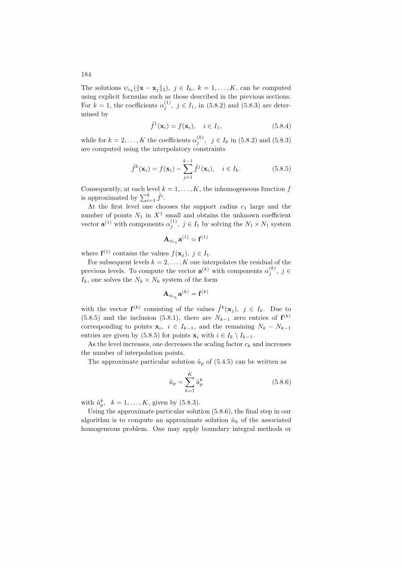
184
The solutions ψck(‖x − xj‖2), j ∈ Ik, k = 1, . . . ,K, can be computed
using explicit formulas such as those described in the previous sections.
For k = 1, the coefficients α(1)j , j ∈ I1, in (5.8.2) and (5.8.3) are deter-
mined by
f1(xi) = f(xi), i ∈ I1, (5.8.4)
while for k = 2, . . . ,K the coefficients α(k)j , j ∈ Ik in (5.8.2) and (5.8.3)
are computed using the interpolatory constraints
fk(xi) = f(xi) −k−1∑
j=1
f j(xi), i ∈ Ik. (5.8.5)
Consequently, at each level k = 1, . . . ,K, the inhomogeneous function f
is approximated by∑k
i=1 fi.
At the first level one chooses the support radius c1 large and the
number of points N1 in X1 small and obtains the unknown coefficient
vector a(1) with components α(1)j , j ∈ I1 by solving the N1 ×N1 system
Aφc1a(1) = f (1)
where f (1) contains the values f(xj), j ∈ I1.
For subsequent levels k = 2, . . . ,K one interpolates the residual of the
previous levels. To compute the vector a(k) with components α(k)j , j ∈
Ik, one solves the Nk ×Nk system of the form
Aφcka(k) = f (k)
with the vector f (k) consisting of the values fk(xj), j ∈ Ik. Due to
(5.8.5) and the inclusion (5.8.1), there are Nk−1 zero entries of f (k)
corresponding to points xi, i ∈ Ik−1, and the remaining Nk − Nk−1
entries are given by (5.8.5) for points xi with i ∈ Ik \ Ik−1.
As the level increases, one decreases the scaling factor ck and increases
the number of interpolation points.
The approximate particular solution up of (5.4.5) can be written as
up =K∑
k=1
ukp (5.8.6)
with ukp, k = 1, . . . ,K, given by (5.8.3).
Using the approximate particular solution (5.8.6), the final step in our
algorithm is to compute an approximate solution uh of the associated
homogeneous problem. One may apply boundary integral methods or

The Method of Particular Solutions 185
the method of fundamental solutions to find the homogeneous solution
uh.
Finally, as in the DRM, one takes u = uh + up as an approximation
to the unique solution u of (5.1.1).
If the algorithm is run bottom–up, users can monitor the full residuals
rK := f − L
(K∑
k=1
ukp
)= f −
K∑
k=1
fk
and stop if a given tolerance on ‖rK‖∞ is reached. If new points for
Xk+1 ⊃ Xk are needed, one can add points y where |rK(y)| is maximal
and thus well above ‖rK‖∞ and the final tolerance. If the scaling is not
changed, this will decrease the residuals under weak assumptions, as is
proven in [SW00, HSZ03] on greedy algorithms. Users should select a
smaller scale for level k+1 only if a reasonable decrease of the residuals
results. If not, the point density at the old level was not large enough,
and the scale should be kept.
With these precautions, the above multiscale algorithm can be run
without difficulty. It ignores the additional homogeneous solution until
it has approximated the particular solution up to some accuracy. On
the downside, it controls only the MPS residual, not the full residual
of the PDE problem. Users will have to wait through all steps of the
algorithm until finally a full approximate solution to the PDE problem
can be displayed.
Thus it is desirable to have a technique which allows us to display an
approximate solution of the problem at each resolution level. This will
be done by the method we describe in the next section.
5.8.3 Multiscale MPS–MFS Algorithm
We now reformulate the previous method in such a way that it calculates
a full approximate solution to the PDE at each scale. The trade–off
is some additional increase in computation costs, because the algorithm
must include the homogeneous solution in each multiscale calculation.
For the starting level k = 1, we first calculate a particular solution u1p
of
Lu1p = f1 in Ω,
using the representations (5.8.3) and (5.8.4). Then u1h is calculated as
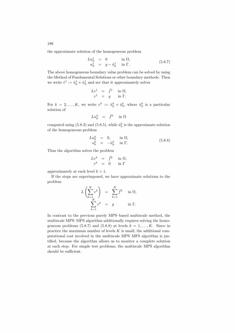
186
the approximate solution of the homogeneous problem
Lu1h = 0 in Ω,
u1h = g − u1
p in Γ.(5.8.7)
The above homogeneous boundary value problem can be solved by using
the Method of Fundamental Solutions or other boundary methods. Then
we write v1 := u1p + u1
h and see that it approximately solves
Lv1 = f1 in Ω,
v1 = g in Γ.
For k = 2, . . . ,K, we write vk := ukp + uk
h, where ukp is a particular
solution of
Lukp = fk in Ω
computed using (5.8.3) and (5.8.5), while ukh is the approximate solution
of the homogeneous problem
Lukh = 0, in Ω,
ukh = −uk
p in Γ.(5.8.8)
Thus the algorithm solves the problem
Lvk = fk in Ω,
vk = 0 in Γ
approximately at each level k > 1.
If the steps are superimposed, we have approximate solutions to the
problem
L
(K∑
k=1
vk
)=
K∑
k=1
fk in Ω,
K∑
k=1
vk = g in Γ.
In contrast to the previous purely MPS–based multiscale method, the
multiscale MPS–MFS algorithm additionally requires solving the homo-
geneous problems (5.8.7) and (5.8.8) at levels k = 1, . . . ,K. Since in
practice the maximum number of levels K is small, the additional com-
putational cost involved in the multiscale MPS–MFS algorithm is jus-
tified, because the algorithm allows us to monitor a complete solution
at each step. For simple test problems, the multiscale MPS algorithm
should be sufficient.
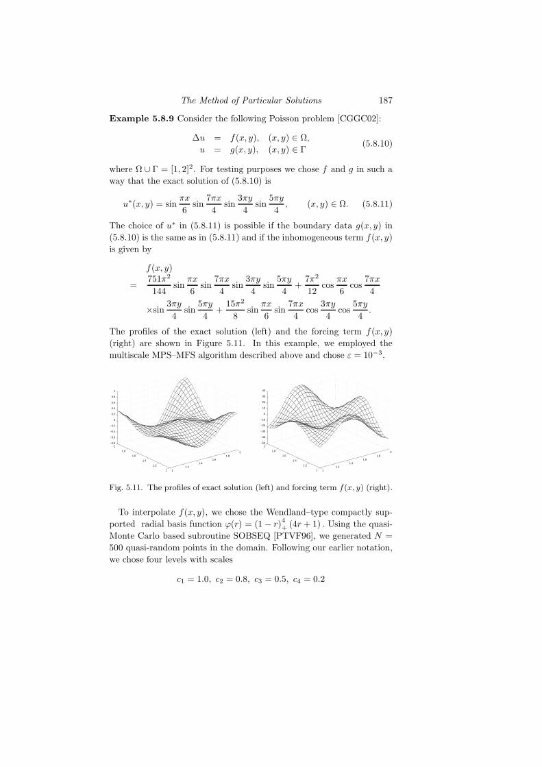
The Method of Particular Solutions 187
Example 5.8.9 Consider the following Poisson problem [CGGC02]:
∆u = f(x, y), (x, y) ∈ Ω,
u = g(x, y), (x, y) ∈ Γ(5.8.10)
where Ω ∪ Γ = [1, 2]2. For testing purposes we chose f and g in such a
way that the exact solution of (5.8.10) is
u∗(x, y) = sinπx
6sin
7πx
4sin
3πy
4sin
5πy
4, (x, y) ∈ Ω. (5.8.11)
The choice of u∗ in (5.8.11) is possible if the boundary data g(x, y) in
(5.8.10) is the same as in (5.8.11) and if the inhomogeneous term f(x, y)
is given by
f(x, y)
= −751π2
144sin
πx
6sin
7πx
4sin
3πy
4sin
5πy
4+
7π2
12cos
πx
6cos
7πx
4
×sin3πy
4sin
5πy
4+
15π2
8sin
πx
6sin
7πx
4cos
3πy
4cos
5πy
4.
The profiles of the exact solution (left) and the forcing term f(x, y)
(right) are shown in Figure 5.11. In this example, we employed the
multiscale MPS–MFS algorithm described above and chose ε = 10−3.
11.2
1.41.6
1.82
1
1.2
1.4
1.6
1.8
2−0.8
−0.6
−0.4
−0.2
0
0.2
0.4
0.6
0.8
1
11.2
1.41.6
1.82
1
1.2
1.4
1.6
1.8
2−50
−40
−30
−20
−10
0
10
20
30
40
Fig. 5.11. The profiles of exact solution (left) and forcing term f(x, y) (right).
To interpolate f(x, y), we chose the Wendland–type compactly sup-
ported radial basis function ϕ(r) = (1 − r)4+ (4r + 1) . Using the quasi-
Monte Carlo based subroutine SOBSEQ [PTVF96], we generated N =
500 quasi-random points in the domain. Following our earlier notation,
we chose four levels with scales
c1 = 1.0, c2 = 0.8, c3 = 0.5, c4 = 0.2

188
and
N1 = 30, N2 = 150, N3 = 300, N4 = 500
and for k = 1, 2, 3, 4 the sets Xk consisted of the first Nk points from
the generated quasi-random points in [1, 2]2.
For k = 1, 2, 3, 4 the sparsity structure (with non–zero entries nzk
and fill–in in %) of the resulting Nk ×Nk matrix Aφckand the absolute
maximum error are given in Table 5.7.
Nk nzk fill–in (%) L∞ error
30 459 51 0.1984
150 9729 43.24 0.59E-3
300 22057 24.50 8.86E-3
500 13299 5.31 8.758E-3
Table 5.7. Sparsity pattern of the interpolation matrix and L∞ error
The profiles of the interpolation error ek = f −∑ki=1 f
k of the forcing
term at each level k = 1, 2, 3, 4 are given in Figure 5.12. The main inter-
est is in the particular solutions obtained at each level. Their profiles are
given in Figure 5.13. As expected, from Figures 5.12 and 5.13, one ob-
serves that ‖ek‖∞ and ||ukp||∞ get smaller as the level increases; i.e. the
scaling factor c shrinks and the number of interpolation points increases.
The profiles of the solution produced at each level, ukp +uk
h, k = 1, 2, 3, 4,
are shown in Figure 5.14. One notes that the contribution of the solution
at levels 3 and 4 is almost insignificant. The overall errors on each level
are shown in Figure 5.15 which are consistent with the solution profile
in Figure 5.14. 2
5.8.4 Series Expansions for Differential Operators
The derivation of particular solutions for Helmholtz-type equations by
solving linear ordinary differential equations as shown in Section 5.7 is
somewhat tedious. In this section, we come back to the technique we
used in Section 5.7.7 to derive particular solutions for polynomial right–
hand sides. Coupled with symbolic software such as MATHEMATICA c©or MAPLE c©, this approach can be applied to more complicated oper-
ators, but it is restricted to the case that φ is a polyharmonic function.

The Method of Particular Solutions 189
11.5
2
1
1.5
2−40
−20
0
20
Level 1
11.5
2
1
1.5
2−4
−2
0
2
Level 2
11.5
2
1
1.5
2−1
−0.5
0
0.5
Level 3
1
1.5
2
1
1.5
2
−1
−0.5
0
0.5
Level 4
Fig. 5.12. Interpolation errors after each level.
11.5
2
1
1.5
2−2
−1
0
Level 1
11.5
2
1
1.5
2−2
−1.5
−1
−0.5
Level 2
11.5
2
1
1.5
2−0.15
−0.1
−0.05
Level 3
1
1.5
2
1
1.5
2
−6
−5
−4
−3
x 10−3
Level 4
Fig. 5.13. Particular solutions produced at each level.

190
11.5
2
1
1.5
2−1
0
1
2
Level 1
11.5
2
1
1.5
2−0.2
0
0.2
Level 2
11.5
2
1
1.5
2−4
−2
0
2
x 10−3
Level 3
1
1.5
2
1
1.5
2
−2
−1
0
1
x 10−3
Level 4
Fig. 5.14. Solution contributed at each level.
11.5
2
1
1.5
20
0.1
0.2
Level 1
11.5
2
1
1.5
20
0.005
0.01
Level 2
11.5
2
1
1.5
20
0.005
0.01
Level 3
1
1.5
2
1
1.5
2
0
0.005
0.01
Level 4
Fig. 5.15. Overall errors after each level.

The Method of Particular Solutions 191
From (5.7.27) and (5.7.33), a particular solution ψ of the Helmholtz
equation
∆ψ − λ2ψ = φ
is given by
ψ =−1
λ2
L∑
k=0
(∆
λ2
)k
φ (5.8.12)
where L is a sufficiently large positive integer. Notice that (5.8.12) is
valid only if φ satisfies ∆L+1φ = 0 for some positive integer L. Following
and generalizing Section 5.7.2, we take fundamental solutions of the
iterated Laplace operator, which are called polyharmonic splines (see
Table 1.3). Like fundamental solutions of the Laplace operator itself,
polyharmonic splines must depend on the space dimension d. In even
space dimensions, they are of the form φ(r) = r2n ln r with L + 1 =
(2n + d)/2 , while they are φ(r) = r2n−1 with L + 1 = (2n − 1 + d)/2
in odd space dimensions. For illustration, let us choose φ = r2 ln r in
(5.8.12) for two dimensions. It is called the thin–plate spline because it
is the fundamental solution of the thin–plate or biharmonic operator ∆2
in two dimensions, leading to L = 1 above. The following Mathematica
code can be used to produce ψ in (5.8.12) symbolically:
ψ [λ ] := Module [ φ, φ = r2 ∗ Log[r]; g = 0;L = 20;
For [ i = 0, i ≤ L, i+ +, g = φ+ g;
φ = Simplify[(
1r ∗ ∂r ∗ (r ∗ ∂r (φ))
)/λ2];
If [φ == 0,Break [ ]] ] ;
g = Simplify[−g/λ2
]];
In the above code, we choose L = 20 which is considered to be sufficiently
large to handle most of the cases. Using the above Mathematica code,
we obtain
ψ [λ] = −4 +(4 + r2λ2
)Log [r]
λ4. (5.8.13)
The particular solution ψ in (5.8.13) is equivalent to the last three terms
in (5.7.14) which we have derived in Section 5.7.2. In (5.8.13), there is
a singular term ln r that needs to be de-singularized. Hence, we still
need to follow the procedure as shown in Section 5.7.2 to cancel the
singularity in (5.8.13).
A similar technique for series expansions of differential operators can
be applied to other types of differential operators such as(∆ − λ2
)2,
∆2 − λ4, product of Helmholtz operators, etc. It is almost impossible

192
to derive the particular solutions for these types of differential operators
using the technique of Section 5.7.2. More specifically, let us consider
the particular solution of the following equation(∆2 − λ4
)ψ = ϕ
which arises in solving the Berger equation. For ϕ = r2 ln r, it is
trivial that
ψ =−r2 ln r
λ4.
For ϕ = r4 ln r, we have
ψ =
r4 ln r
λ4− 4 ln r + 96
λ8− 64K0(λr)
λ8, r > 0,
1
λ8
(64γ + ln
(λ
2
)− 96
), r = 0.
For ϕ = r6 ln r, we have
ψ = − 1
λ4
(r6 ln r +
1
λ4
(576r2 ln r + 480
)).
The fundamental solution for the operator ∆2 − λ4 in 2D can be found
in Table 4.1. With particular solution and fundamental solution both
available, the Berger equation can be solved without much effort.
5.8.5 Particular Solutions from Fundamental Solutions
We now provide a technique for constructing particular solutions to
Laplace or Helmholtz equations starting from fundamental solutions of
the Helmholtz equation [AC05].
We take a fundamental solution ψλ of the modified Helmholtz equa-
tion, i.e.
(∆ − λ)ψλ = −δ (5.8.14)
where λ ∈ IR and
ψλ(r) =
1
2πK0(
√λr), if λ > 0
−1
2πln(r), if λ = 0
i
4H
(1)0 (
√−λr), if λ < 0
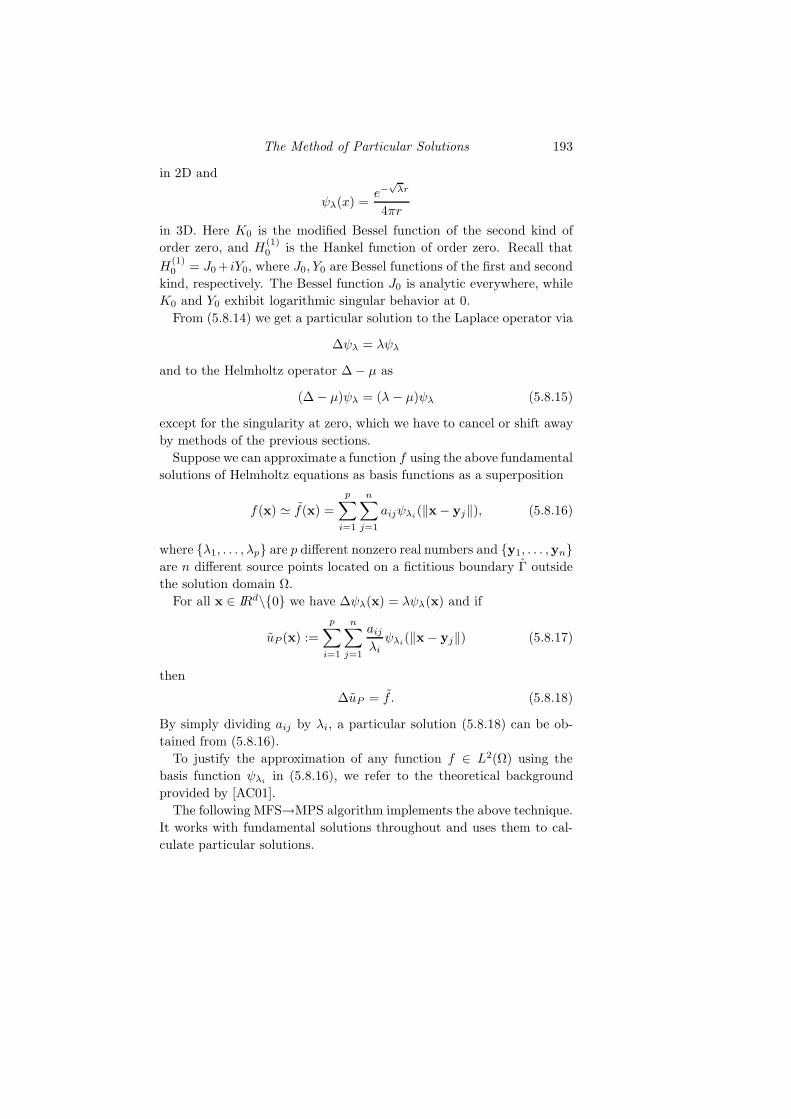
The Method of Particular Solutions 193
in 2D and
ψλ(x) =e−
√λr
4πr
in 3D. Here K0 is the modified Bessel function of the second kind of
order zero, and H(1)0 is the Hankel function of order zero. Recall that
H(1)0 = J0 + iY0, where J0, Y0 are Bessel functions of the first and second
kind, respectively. The Bessel function J0 is analytic everywhere, while
K0 and Y0 exhibit logarithmic singular behavior at 0.
From (5.8.14) we get a particular solution to the Laplace operator via
∆ψλ = λψλ
and to the Helmholtz operator ∆ − µ as
(∆ − µ)ψλ = (λ − µ)ψλ (5.8.15)
except for the singularity at zero, which we have to cancel or shift away
by methods of the previous sections.
Suppose we can approximate a function f using the above fundamental
solutions of Helmholtz equations as basis functions as a superposition
f(x) ≃ f(x) =
p∑
i=1
n∑
j=1
aijψλi(‖x− yj‖), (5.8.16)
where λ1, . . . , λp are p different nonzero real numbers and y1, . . . ,ynare n different source points located on a fictitious boundary Γ outside
the solution domain Ω.
For all x ∈ IRd\0 we have ∆ψλ(x) = λψλ(x) and if
uP (x) :=
p∑
i=1
n∑
j=1
aij
λiψλi
(‖x − yj‖) (5.8.17)
then
∆uP = f . (5.8.18)
By simply dividing aij by λi, a particular solution (5.8.18) can be ob-
tained from (5.8.16).
To justify the approximation of any function f ∈ L2(Ω) using the
basis function ψλiin (5.8.16), we refer to the theoretical background
provided by [AC01].
The following MFS→MPS algorithm implements the above technique.
It works with fundamental solutions throughout and uses them to cal-
culate particular solutions.
194
MFS→MPS Algorithm
(i) Choose m collocation points x1, ...,xm in the domain Ω,
(ii) choose n source points y1, ...,yn on the fictitious boundary Γ,
(iii) choose p nonzero frequencies λ1, ..., λp ∈ IR,
(iv) define the m × (np) matrix M
M := (M1, . . . ,Mp)
consisting of p blocks
Mi := (ψλi(‖xj − yk‖))1≤j≤m, 1≤k≤n , 1 ≤ i ≤ p
of size m× n each,
(v) solve the (np) × (np) least-squares system
MTMa = MT f ,
where f = (f(x1), . . . , f(xm))T .
The vector solution a = (a11, . . . , an1, . . . , a1p, . . . , anp) ∈ IRnp will
provide an approximation of f in the form
f(x) =
p∑
k=1
n∑
j=1
ajkψλk(‖x − yj‖). (5.8.19)
Since we just want to approximate a real–valued function, there is no
need to consider complex fundamental solutions. We can simply use the
real part of the complex fundamental solution as our basis function. For
instance, in the 2D case, it will be sufficient to use J0, which is a regular
function, as the basis. As a result, this allows us to admit points yj
inside Ω. This means that we can take our approximations from the
space
spanJ0(√−λ‖x− y‖)|Ω : y ∈ IR2, λ ∈ (−∞, 0].
Similarly, in the 3D case, it suffices to consider
span
sin(
√−λ‖x − y‖)‖x − y‖ |Ω : y ∈ IR3, λ ∈ (−∞, 0]
.

The Method of Particular Solutions 195
5.8.6 Inhomogeneous Helmholtz Equation
A similar technique can be applied to find a particular solution of the
inhomogeneous Helmholtz-type equation
∆u− µu = f
for any µ ∈ IR. We already pointed this out in (5.8.15). In fact, assuming
that we have an approximation of f given by f in formula (5.8.19), then
from
uP (x) =
p∑
k=1
n∑
j=1
ajk
λk − µψλk
(‖x − yj‖) (5.8.20)
with λ1, ..., λp 6= µ, we get
(∆ − µ)uP (x) =
p∑
k=1
n∑
j=1
ajk
λk − µ(∆ − µ)ψλk
(‖x − yj‖)
=
p∑
k=1
n∑
j=1
ajk
λk − µ(λk − µ)ψλk
(‖x − yj‖)
= f(x).
Once we have obtained the approximation of the particular solution uP
in (5.8.20), we must then solve the problem
∆uH − µuH = 0, in Ω,
BuH = g − BuP , on Γ,
and this can be done using the classical method of fundamental solutions.
We must keep in mind that the condition on the boundary is now given
with an approximated uP and a poor approximation of uP might carry
more significant errors to uH .
We recall that the solution obtained by the method of fundamental
solutions will now be written in the form
uH(x) =m∑
j=1
ajψµ(‖x − yj‖).
Example 5.8.21 We consider the Poisson problem given in Example
5.8.9. To approximate the forcing term f(x, y) and thus the particular
solution, we used the Bessel function J0 as the basis function. We chose
400 quasi-random interior points in an extended domain [0.85, 2.15] ×[0.85, 2.15] and 40 evenly distributed source points on the fictitious
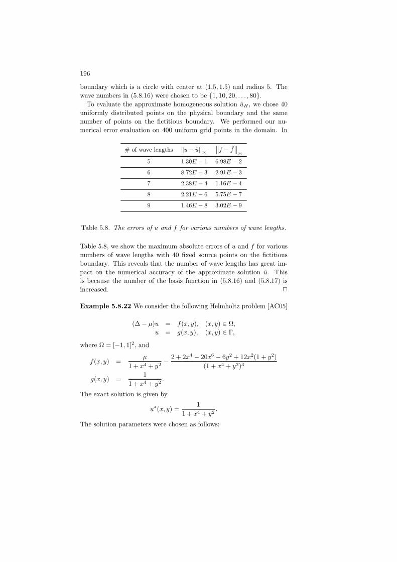
196
boundary which is a circle with center at (1.5, 1.5) and radius 5. The
wave numbers in (5.8.16) were chosen to be 1, 10, 20, . . . , 80.To evaluate the approximate homogeneous solution uH , we chose 40
uniformly distributed points on the physical boundary and the same
number of points on the fictitious boundary. We performed our nu-
merical error evaluation on 400 uniform grid points in the domain. In
# of wave lengths ‖u− u‖∞∥∥f − f
∥∥∞
5 1.30E − 1 6.98E − 2
6 8.72E − 3 2.91E − 3
7 2.38E − 4 1.16E − 4
8 2.21E − 6 5.75E − 7
9 1.46E − 8 3.02E − 9
Table 5.8. The errors of u and f for various numbers of wave lengths.
Table 5.8, we show the maximum absolute errors of u and f for various
numbers of wave lengths with 40 fixed source points on the fictitious
boundary. This reveals that the number of wave lengths has great im-
pact on the numerical accuracy of the approximate solution u. This
is because the number of the basis function in (5.8.16) and (5.8.17) is
increased. 2
Example 5.8.22 We consider the following Helmholtz problem [AC05]
(∆ − µ)u = f(x, y), (x, y) ∈ Ω,
u = g(x, y), (x, y) ∈ Γ,
where Ω = [−1, 1]2, and
f(x, y) =µ
1 + x4 + y2− 2 + 2x4 − 20x6 − 6y2 + 12x2(1 + y2)
(1 + x4 + y2)3
g(x, y) =1
1 + x4 + y2.
The exact solution is given by
u∗(x, y) =1
1 + x4 + y2.
The solution parameters were chosen as follows:

The Method of Particular Solutions 197
• 400 evenly distributed collocation points in an extended domain
W ⊃ Ω where W = [−1.2, 1.2]2.
• 16 source points evenly distributed
in the extended domain [−1.1, 1.1]2.
• 8 frequencies:
λk8k=1 = −1,−4,−9,−16,−25,−36,−49,−64.
Note that we shall use values of µ different from these frequencies.
This information is required to approximate f and uP . Note that we
considered an extended domain W to produce a better approximation
of f in Ω.
To approximate the homogeneous solution uH , we chose the following
parameters:
• 40 collocation points on the physical boundary Γ.
• 40 source points on the fictitious boundary Γ which is a circle
with center at (0, 0) and radius 5.
In this example, we placed the source points inside the domain for the
approximation of particular solutions. This distribution of the colloca-
tion and source points for the MFS→MPS algorithm on page 194 and
the traditional method of fundamental solutions are shown in Figure
5.16. This does not present a singularity problem because we have used
the nonsingular part of the Bessel function J0 as the basis. In fact,
we could have also placed the 16 source points on a circle outside the
domain. Now consider the Helmholtz equation with µ = −18. Using
−1.5 −1 −0.5 0 0.5 1 1.5−1.5
−1
−0.5
0
0.5
1
1.5
−6 −4 −2 0 2 4 6−6
−4
−2
0
2
4
6
Fig. 5.16. Source points (circle) and collocation points (dot) using MFS→MPSfor evaluating uP (left) and the traditional method of fundamental solutionsfor evaluating uH (right).

198
the previous data with interior point sources, we obtained about 0.5%
maximum relative errors in the function approximation and about 0.1%
maximum relative errors in the approximation of the solution of the
Helmholtz equation. The profiles of the relative errors of f and u are
shown in Figure 5.17.
-1-0.5
0
0.5
1
-1
-0.5
00.5
1
0
0.02
0.04
0.06
-1-0.5
0
0.5
1
-1
-0.5
00.5
1
-1-0.5
0
0.5
1
-1
-0.50
0.51
0
0.0005
0.001
-1-0.5
0
0.5
1
-1
-0.50
0.51
Fig. 5.17. The profiles of relative errors of f and u.
2
5.8.7 Fast Solution of the MFS for Modified Helmholtz
Equations
In the formulation of the Method of Fundamental Solutions, we usually
obtain a dense matrix which is expensive to handle, especially for the
3D case. But for the modified Helmholtz equation, we have noticed that
its fundamental solutions K0(λr) in 2D and exp(−λr)/r in 3D have ex-
ponential decay. As a result, when λr is sufficiently large, most of the
entries of the formulated matrix become so small that they can be con-
sidered as negligible and thus can be truncated without loss of numerical
accuracy. After the truncation, the new resulting matrix becomes sparse
and can be treated efficiently using some sparse solver.
The wave number λ inK0(λr) or exp(−λr)/r depends on the governed
equation, and r depends on the size and geometric shape of the domain.
Thus the efficiency of the algorithm depends on the combination of these
two factors.
Example 5.8.23 To be more specific, we consider the following modified
Helmholtz equation with Dirichlet boundary condition
∆u− λ2u = (1 − λ2)(ex + ey), (x, y) ∈ Ω,
u = ex + ey, (x, y) ∈ Γ,(5.8.24)

The Method of Particular Solutions 199
where Ω is a bounded domain and Γ satisfies the following parametric
equation:
x = r(θ) cos θ, y = r(θ) sin θ,
r(θ) =
√cos2 2θ +
√1.1 − sin2 2θ, 0 ≤ θ ≤ 2π.
By the method of particular solutions, we reduce (5.8.24) to the following
homogeneous equation:
∆v − λ2v = 0, (x, y) ∈ Ω,
v = ex + ey − up, (x, y) ∈ Γ.
Here we choose λ2 = 1000. To evaluate the approximate particular so-
lution, 100 evenly distributed grid points were chosen in the extended
domain [−1.5, 1.5] × [−1, 1] plus 100 boundary points which were also
used as the collocation points for the method of fundamental solutions.
The distribution of these points is shown in Figure 5.18. Furthermore,
third order polyharmonic splines were chosen as the basis function to
interpolate the forcing term of (5.8.24). Let A be the coefficient ma-
−1.5 −1 −0.5 0 0.5 1 1.5−1
−0.8
−0.6
−0.4
−0.2
0
0.2
0.4
0.6
0.8
1
Fig. 5.18. The distribution of interpolation points and collocation points.
trix in the formulation of the method of fundamental solutions. The
maximum and minimum coefficients of A are εmax = 5.346× 10−92 and
εmin = 2.157×10−131 respectively. We notice that there is a wide margin

200
between εmax and εmin. Let the truncation value be ε. This means
aij =
0, aij < ε,
aij , i = j,
aij , aij ≥ ε,
where aij is the entry in A. To ensure the matrix is nonsingular after
the truncation, we should always keep the diagonal entries of A. For
ε = 10−95, there are only 412 nonzero entries in A. This means 96% of
the entries of A were truncated. The profile of nonzero entries of A is
shown in Figure 5.19. Surprisingly, the maximum absolute errors of the
solution (3.35×10⁻⁵) before and after the truncation are identical. The
absolute maximum error were computed on the 60 test points located
on the boundary. We also observe that the condition numbers of A
before and after the truncation are 1035 and 1018 respectively. The
improvement of the condition number does not affect the final result.
0 10 20 30 40 50 60 70 80 90 100
0
10
20
30
40
50
60
70
80
90
100
nz = 412
Fig. 5.19. The profile of nonzero entries of A.
Using the same setting as just described, some further numerical re-
sults using various wave number λ2 are given in Table 5.9 where L∞denotes the absolute maximum error. In all cases, the L∞ are exactly
the same before and after the truncation. The last column of Table 5.9
shows the condition numbers before and after the truncation.
2
One of the important applications of using modified Helmholtz equa-

The Method of Particular Solutions 201
λ2 εmin εmax ε L∞ #( 6= 0) Cond. #
10 2.60E-10 2.54E-14 2.60E-11 5.49E-2 12.32% 1020 : 109
100 4.58E-30 1.41E-42 4.58E-32 1.023E-3 7.72% 1023 : 108
500 1.68E-65 2.22E-93 1.68E-67 8.55E-5 3.76% 1029 : 1013
Table 5.9. Numerical results for various values of λ2.
tions is in the area of time–dependent problems which will be described
in the next chapter. The above described fast solution algorithm can be
applied to the time–dependent problems in case of large wave numbers.
5.9 Solving Large Problems on Circular Points
In case of specially distributed interpolation or collocation points, a
surprisingly effective numerical technique for reconstruction of functions
from data can be applied [KCS07]. Though it could also be presented at
the end of Chapter 2, we present it here due to its applicability within
the Method of Particular Solutions.
Assume that the forcing term of a two–dimensional PDE is given as a
global formula, and assume that we want to approximate it by a linear
combination of particular solutions. Then we are free to choose the data
points for reconstruction, and we can make use of this freedom.
We choose a large circle around the domain in question, and choose
a number m of concentric circles within this circle. On each circle, we
choose the same number n of equidistant points. In this way, the resul-
tant interpolation matrix has the special feature of blocks of circulant
matrices due to symmetry. The circulant matrix has many attractive
properties which allow us to solve linear equations that contains them
efficiently through the use of the fast Fourier transform.
For simplicity, assume that 12 = 3 · 4 interpolation points are dis-
tributed in the circular form with n = 4 equidistant points on m = 3
circles as shown in Figure 5.20.
We focus on reconstruction by interpolation, and we let f(x) be the
function to be interpolated. By the usual radial basis function interpo-

202
1
3
4
5
67
8
2
910
1112
Fig. 5.20. Distribution of 12 circulant points.
lation scheme as shown in Chapter 1.1, we have
f(x) ≃ f(x) =
12∑
j=1
ajϕ (‖x − xj‖) .
As the standard linear system for interpolation, we have
f(xi) = f(xi) =
12∑
j=1
ajϕ (‖xi − xj‖) , 1 ≤ i ≤ 12, (5.9.1)
which can be formulated in the matrix form Aϕa = f where
a = (a1, a2, . . . , a12)T,
f = (f(x1), f(x2), . . . , f(x12))T,
and
Aϕ =
ϕ1,1 ϕ1,2 · · · ϕ1,12
ϕ2,1 ϕ2,2 · · · ϕ2,12
......
. . ....
ϕ1,12 ϕ12,12 · · · ϕ12,12
,
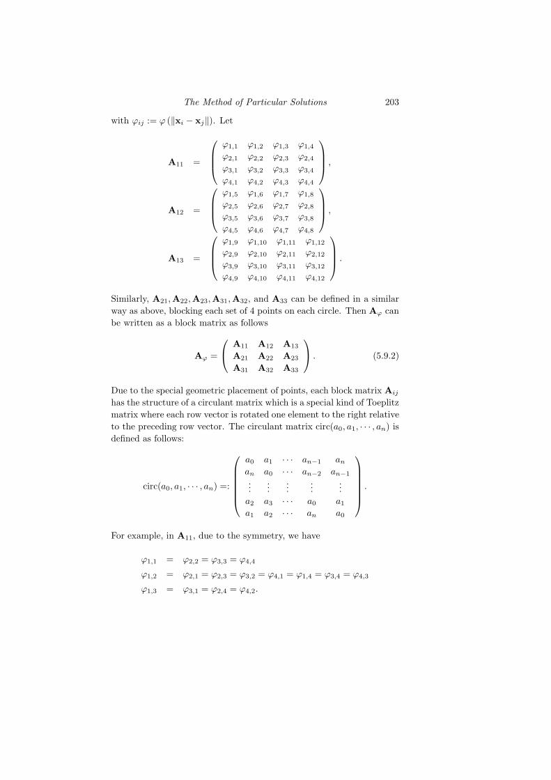
The Method of Particular Solutions 203
with ϕij := ϕ (‖xi − xj‖). Let
A11 =
ϕ1,1 ϕ1,2 ϕ1,3 ϕ1,4
ϕ2,1 ϕ2,2 ϕ2,3 ϕ2,4
ϕ3,1 ϕ3,2 ϕ3,3 ϕ3,4
ϕ4,1 ϕ4,2 ϕ4,3 ϕ4,4
,
A12 =
ϕ1,5 ϕ1,6 ϕ1,7 ϕ1,8
ϕ2,5 ϕ2,6 ϕ2,7 ϕ2,8
ϕ3,5 ϕ3,6 ϕ3,7 ϕ3,8
ϕ4,5 ϕ4,6 ϕ4,7 ϕ4,8
,
A13 =
ϕ1,9 ϕ1,10 ϕ1,11 ϕ1,12
ϕ2,9 ϕ2,10 ϕ2,11 ϕ2,12
ϕ3,9 ϕ3,10 ϕ3,11 ϕ3,12
ϕ4,9 ϕ4,10 ϕ4,11 ϕ4,12
.
Similarly, A21,A22,A23,A31,A32, and A33 can be defined in a similar
way as above, blocking each set of 4 points on each circle. Then Aϕ can
be written as a block matrix as follows
Aϕ =
A11 A12 A13
A21 A22 A23
A31 A32 A33
. (5.9.2)
Due to the special geometric placement of points, each block matrix Aij
has the structure of a circulant matrix which is a special kind of Toeplitz
matrix where each row vector is rotated one element to the right relative
to the preceding row vector. The circulant matrix circ(a0, a1, · · · , an) is
defined as follows:
circ(a0, a1, · · · , an) =:
a0 a1 · · · an−1 an
an a0 · · · an−2 an−1
......
......
...
a2 a3 · · · a0 a1
a1 a2 · · · an a0
.
For example, in A11, due to the symmetry, we have
ϕ1,1 = ϕ2,2 = ϕ3,3 = ϕ4,4
ϕ1,2 = ϕ2,1 = ϕ2,3 = ϕ3,2 = ϕ4,1 = ϕ1,4 = ϕ3,4 = ϕ4,3
ϕ1,3 = ϕ3,1 = ϕ2,4 = ϕ4,2.
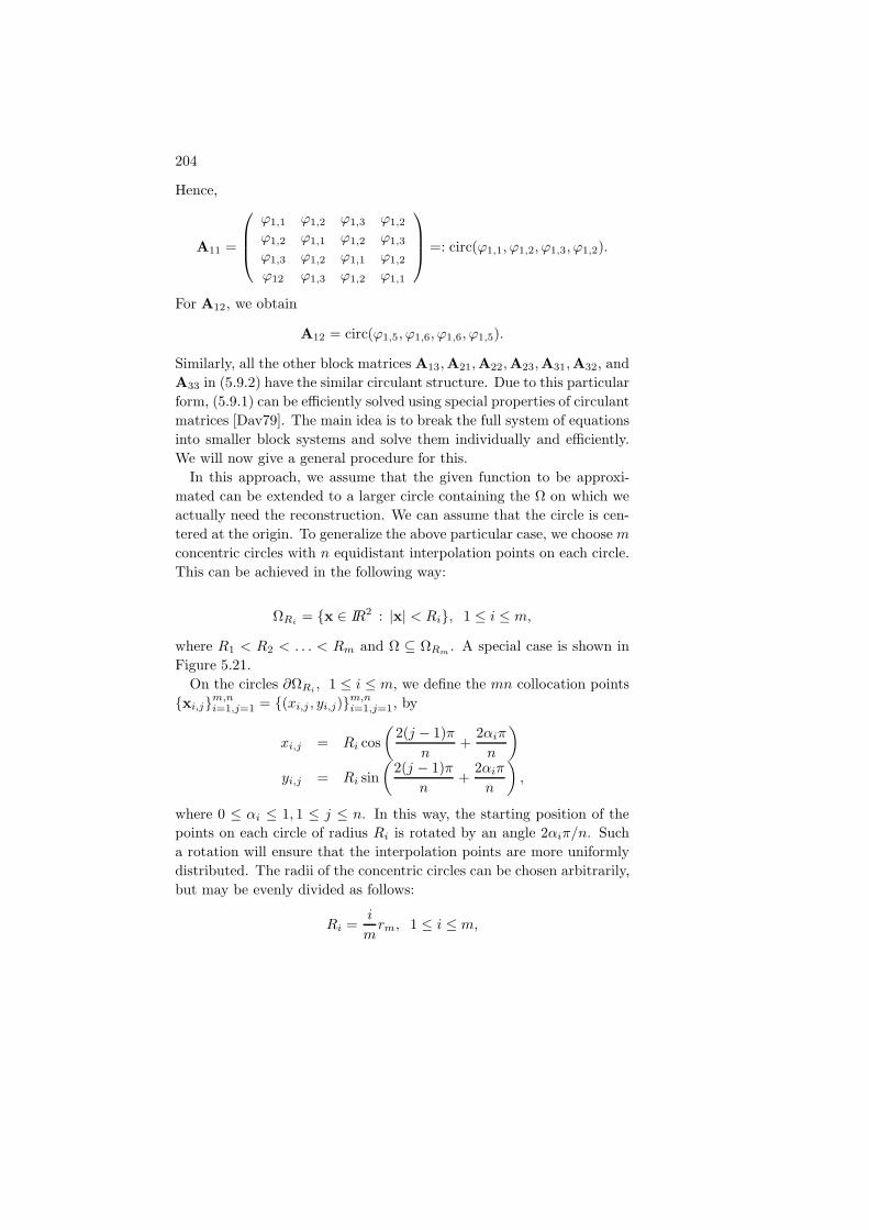
204
Hence,
A11 =
ϕ1,1 ϕ1,2 ϕ1,3 ϕ1,2
ϕ1,2 ϕ1,1 ϕ1,2 ϕ1,3
ϕ1,3 ϕ1,2 ϕ1,1 ϕ1,2
ϕ12 ϕ1,3 ϕ1,2 ϕ1,1
=: circ(ϕ1,1, ϕ1,2, ϕ1,3, ϕ1,2).
For A12, we obtain
A12 = circ(ϕ1,5, ϕ1,6, ϕ1,6, ϕ1,5).
Similarly, all the other block matrices A13,A21,A22,A23,A31,A32, and
A33 in (5.9.2) have the similar circulant structure. Due to this particular
form, (5.9.1) can be efficiently solved using special properties of circulant
matrices [Dav79]. The main idea is to break the full system of equations
into smaller block systems and solve them individually and efficiently.
We will now give a general procedure for this.
In this approach, we assume that the given function to be approxi-
mated can be extended to a larger circle containing the Ω on which we
actually need the reconstruction. We can assume that the circle is cen-
tered at the origin. To generalize the above particular case, we choose m
concentric circles with n equidistant interpolation points on each circle.
This can be achieved in the following way:
ΩRi= x ∈ IR2 : |x| < Ri, 1 ≤ i ≤ m,
where R1 < R2 < . . . < Rm and Ω ⊆ ΩRm. A special case is shown in
Figure 5.21.
On the circles ∂ΩRi, 1 ≤ i ≤ m, we define the mn collocation points
xi,jm,ni=1,j=1 = (xi,j , yi,j)m,n
i=1,j=1, by
xi,j = Ri cos
(2(j − 1)π
n+
2αiπ
n
)
yi,j = Ri sin
(2(j − 1)π
n+
2αiπ
n
),
where 0 ≤ αi ≤ 1, 1 ≤ j ≤ n. In this way, the starting position of the
points on each circle of radius Ri is rotated by an angle 2αiπ/n. Such
a rotation will ensure that the interpolation points are more uniformly
distributed. The radii of the concentric circles can be chosen arbitrarily,
but may be evenly divided as follows:
Ri =i
mrm, 1 ≤ i ≤ m,

The Method of Particular Solutions 205
Fig. 5.21. The domain of the function and the circular interpolation points.
where rm is the radius of the largest circle. In Figure 5.21, we present a
typical distribution of collocation points with n = 20,m = 20, rmax = 1,
and αi = 0 for i = 1, 3, · · · , 19, αi = 0.5, for i = 2, 4, · · · , 20.
For the mn circular points given above, the collocation equations
(5.9.1) can be generalized to the following system
f(xi,k) =
m∑
ℓ=1
n∑
j=1
aℓ,jϕ(‖xℓ,j −xi,k‖2), 1 ≤ i ≤ m, 1 ≤ k ≤ n. (5.9.3)
In matrix form, we have
Aϕa = f (5.9.4)
where the mn×mn matrix Aϕ has the structure
Aϕ =
A11 A12 . . . A1,m
A21 A22 . . . A2,m
......
. . ....
Am1 Am2 . . . Am,m
(5.9.5)

206
where each of the n× n submatrices Ai,ℓ is circulant due to
Ai,ℓ = (ϕ(‖xi,k − xℓ,j‖2))1≤j,k≤n
= (ϕ(‖Rk−1xi,1 −Rj−1xℓ,1‖2))1≤j,k≤n
= (ϕ(‖Rk−1(xi,1 −Rj+n−kxℓ,1)‖2))1≤j,k≤n
= (ϕ(‖xi,1 −Rj+n−kxℓ,1‖2))1≤j,k≤n
= circ(ϕ ‖xi,1 − xℓ,1‖2 , . . . , ϕ ‖xi,1 − xℓ,n‖2), 1 ≤ i, ℓ ≤ m,
if we denote rotation by an angle of 2π/n by R. Also, we have
f(i−1)n+j = f(xi,j), 1 ≤ i ≤ m, 1 ≤ j ≤ n.
Altogether, our system is block–circulant, and such systems have an
efficient solution procedure which we outline here.
It is known that any circulant matrix can be diagonalized in the fol-
lowing way. If C = circ(c1, . . . , cn), then
C = U∗DU
where D = diag(d1, . . . , dn), dj =∑n
k=1 ckω(k−1)(j−1), and the n × n
matrix U is the matrix arising in the Discrete Fourier Transform,
and is the conjugate of the matrix (see [Dav79])
U∗ =1
n1/2
1 1 1 . . . 1
1 ω ω2 . . . ωn−1
1 ω2 ω4 . . . ω2(n−1)
......
......
1 ωn−1 ω2(n−1) . . . ω(n−1)(n−1)
,
with ω = e2πι/n.
Next, we denote the matrix tensor product by ⊗. The tensor product
of the m× n matrix V and the ℓ× k matrix W is the mℓ× nk matrix
[Mey00]
V ⊗ W =
v11W v12W · · · v1nW
v21W v22W · · · v2nW...
.... . .
...
vm1W vm2W · · · vmnW
.
We therefore premultiply the system (5.9.4) by the block diagonal mn×mn matrix Im ⊗ U and, using the fact that U is unitary, we have
(Im ⊗ U)Aϕ (Im ⊗ U∗) (Im ⊗ U)a = (Im ⊗ U) f ,

The Method of Particular Solutions 207
since (Im ⊗ U∗) (Im ⊗ U) = Imn. This yields
Aϕa = f , (5.9.6)
where a = (Im ⊗ U)a , f = (Im ⊗ U) f ,
Aϕ =
D11 D12 . . . D1,m
D21 D22 . . . D2,m
......
. . ....
Dm1 Dm2 . . . Dm,m
(5.9.7)
and each n × n submatrix Dk,ℓ is diagonal and symmetric. If the sub-
matrix Ai,ℓ of Aϕ in (5.9.5) is circulant, i.e.
Ai,ℓ = circ(ci,ℓ1 , . . . , ci,ℓn )
=
ci,ℓ1 ci,ℓ2 ci,ℓ3 . . . ci,ℓn
ci,ℓn ci,ℓ1 ci,ℓ2 . . . ci,ℓn−1
ci,ℓn−1 ci,ℓn ci,ℓ1 . . . ci,ℓn−2...
......
. . ....
ci,ℓ2 ci,ℓ3 ci,ℓ4 . . . ci,ℓ1
,
then the corresponding submatrix is Di,ℓ = diag(di,ℓ1 , . . . , di,ℓ
n ), where
di,ℓj =
n∑
k=1
ci,ℓk ω(k−1)(j−1), 1 ≤ j ≤ n.
Equipped with this important property, the system (5.9.6) can be de-
composed into n complex systems of equations, each of size m×m, i.e.
Ej aj = fj , 1 ≤ j ≤ n, (5.9.8)
where
(Ej)i,ℓ = di,ℓj , 1 ≤ i, ℓ ≤ m, 1 ≤ j ≤ n,
(fj)i = f(i−1)n+j = f(xi,j), 1 ≤ j ≤ n, 1 ≤ i ≤ m,
and
(aj)i = a(i−1)n+j = ai,j , 1 ≤ j ≤ n, 1 ≤ i ≤ m.
In other words, the entries (i, ℓ) of the matrix Ej are formed by extract-
ing the jth diagonal entry of each Di,ℓ.

208
We summarize the above procedure in the following matrix decom-
position algorithm for the evaluation of coefficients of a = ajmnj=1 in
(5.9.3):
Algorithm of Matrix Decomposition
Step 1 Compute f = (Im ⊗ U) f.
Step 2 Evaluate the m2n elements di,ℓj , 1 ≤ i, ℓ ≤ m, 1 ≤ j ≤ n.
Step 3 Solve the m×m systems Ej aj = fj , 1 ≤ j ≤ n.
Step 4 Compute a = (Im ⊗ U∗) a.
Due to the form of the unitary matrix U, the operation in Step 1
can be efficiently performed using the Fast Fourier Transform (FFT).
The operation count then is O(mn lnn). Similarly, because of the form
of the matrix U∗, the operation in Step 4 can be carried out via inverse
FFTs at a cost of order O(mn lnn).
In Step 3, we need to solve n complex linear m×m systems. Gauss
elimination with partial pivoting can be employed at a cost of O(nm3)
operations. In Step 2, we apply FFTs at a cost of O(m2n lnn) opera-
tions.
It is noteworthy that in this algorithm we do not have to physically
store the interpolation points. All we need is to store the diagonal ele-
ments of Dij as shown in (5.9.7). When m and n are large, this results
in substantial saving in storage. Furthermore, the diagonal entries of
Dij are conjugate complex numbers. As a result, we need to store only
half of them in the computer memory. The other half of the conjugate
numbers can be generated when needed. This also presents a great sav-
ing in memory space on a computer. This allows us to solve large-scale
problems of this specific form without using the domain decomposition
method or any other of the techniques described in Section 2.8.
Some limitations of the above algorithm include the fact that it is
not suitable for the interpolation of data at fixed scattered locations. If
working on a non–circular domain, we also need to be able to smoothly
extend the function to be reconstructed to the exterior of the domain un-
der consideration. Furthermore, radial basis functions with polynomial
augmentation cannot be used.
Example 5.9.9 Here we perform some numerical tests [KCS07] by using
two of the benchmark functions of R. Franke [Fra82] on the unit square.

The Method of Particular Solutions 209
Two of these test functions are given as follows:
F1(x, y) =3eh1(x,y)
4+
3eh2(x,y)
4+eh3(x,y)
2− eh4(x,y)
5
where
h1(x, y) =−1
4
((9x− 2)2 + (9y − 2)2
),
h2(x, y) =−1
49(9x+ 1)2 − 1
10(9y + 1)2,
h3(x, y) =−1
4(9x− 7)2 − 1
4(9y − 3)2,
h4(x, y) = −(9x− 4)2 − (9y − 7)2,
F2(x, y) = 19 [tanh(9y − 9x) + 1] .
00.2
0.40.6
0.81
00.2
0.40.6
0.81
−0.2
0
0.2
0.4
0.6
0.8
1
1.2
XY
Z
00.2
0.40.6
0.81
0
0.2
0.4
0.6
0.8
10
0.05
0.1
0.15
0.2
0.25
XY
Z
Fig. 5.22. Profiles of test functions F1 and F2.
We denote by m the number of concentric circles, by n the number of
interpolation points that are evenly distributed on each circle, and by
rm the radius of the largest circle centered at (0.5, 0.5) which covers the
unit square [0, 1]×[0, 1]. We used multiquadrics with a scaling constant
c as in (2.6.1).
We chose 400 evenly distributed test points in the unit square for
the evaluation of the absolute maximum error. The numerical results in
Table 5.10 were obtained by choosing various parameters c, rm,m, and n.
Consequently, the total number of interpolation points used for m = n =
90, 110, 130, 150 is 8100, 12100, 16900, and 22500, respectively. The
accuracy of the results presented in Table 5.10 is excellent. Furthermore,
the matrix decomposition algorithm is also highly efficient. Using a
Pentium 4 (3.19GHZ) PC, the CPU time for various m and n is also
listed in Table 5.10.

210
m n c F1
(∥∥∥f − f∥∥∥∞
)F2
(∥∥∥f − f∥∥∥∞
)CPU (seconds)
90 90 0.1 1.17E − 09 2.18E − 09 1.57
110 110 0.1 2.10E − 10 2.81E − 10 2.56
130 130 0.09 5.43E − 11 5.41E − 11 3.92
150 150 0.07 2.92E − 11 4.08E − 11 5.67
Table 5.10. Absolute maximum errors for the two test functions with
rm = 1.0.
As is well known, a challenge when using radial basis functions is
the limitation in the number of interpolation points we can use. Here
we wish to make m and n as large as possible. To break the barrier
of memory limitation, further consideration of memory management is
required. Instead of storing all the Ej, j = 1, . . . , n in (5.9.8), we
simply subdivide n into k equal groups, depending on the capacity of
the computer, and store Ej accordingly. We then solve these group by
group. The price one pays for this is the additional evaluation of Dij
in (5.9.7) k times. In this way, we use computing time in exchange
for memory space. The number k can be adjusted depending on the
computer hardware system used. As shown in Table 5.11, we managed
to reachm = 250, n = 400 with k = 2 (i.e. 100, 000 interpolation points)
without encountering problems. Without memory management (k = 1),
the CPU times in Table 5.11 are 26.92, 29.75, 44.56 respectively. Thus,
this method enables us to solve large–scale problems on a standard PC.
Here we used multiquadrics with a scale factor c = 0.04. The better
accuracy with larger rm is consistent with the results in Table 5.10.
Since we solve a much smaller m×m system n times instead of solving
a large mn×mn system, the algorithm is suitable for parallel implemen-
tation. The computer running time can thus be significantly reduced.
2
For engineering applications, it is important to have good approxima-
tions of the gradient and second derivatives of a given function. But it
is known that numerical differentiation is inherently ill-posed. A small
change of the function may cause significant change in its derivatives.
The approximation of the first derivative of a given function is unstable
by any numerical algorithm, although the instability is often manage-

The Method of Particular Solutions 211
m n∥∥∥f − f
∥∥∥∞
CPU time (seconds)
250 250 2.68E-11 43.53
250 300 4.07E-11 47.15
250 400 7.29E-11 54.23
Table 5.11. Absolute maximum error and CPU time for F1 with
c = 0.04 and rm = 1.0.
able. The task of approximating higher derivatives is even more chal-
lenging. Thus we also treat derivative evaluation here, but we remind
the reader that interpolation of smooth functions by smooth radial basis
functions will always yield good approximations also to the derivatives
of the given function (see Section 2.3).
Example 5.9.10 In this example, we further consider the approxima-
tion of the first and second partial derivatives of the following function
[KCS07]:
f(x, y) := F3(x, y) := x exp(−x2 − y2), (x, y) ∈ [0, 1]× [0, 1] .
Then,
∇f(x, y) =
((1 − 2x2) exp(−x2 − y2), 2xy exp(−x2 − y2)
),
∂2f
∂x2(x, y) = (4x3 − 6x) exp(−x2 − y2),
∂2f
∂y2(x, y) = −(2x− 4xy2) exp(−x2 − y2).
To approximate the partial derivatives of a given function, we take
the partial derivatives of the basis function in (5.9.3); i.e. ,
∂f
∂x(x, y) ≃ ∂f
∂x(x, y)) =
mn∑
j=1
aj∂ϕj
∂x(x, y),
∂2f
∂x2(x, y) ≃ ∂2f
∂x2(x, y) =
mn∑
j=1
aj∂2ϕj
∂x2(x, y),

212
∂f
∂y(x, y) ≃ ∂f
∂y(x, y) =
mn∑
j=1
aj∂ϕj
∂y(x, y),
∂2f
∂y2(x, y) ≃ ∂2f
∂y2(x, y) =
mn∑
j=1
aj∂2ϕj
∂y2(x, y),
with
ϕj(x, y) =√ρ2
j(x, y) + c2, ρ2j(x, y) := (x− xj)
2 + (y − yj)2
and∂ϕj
∂x=
x− xj√ρ2
j + c2,
∂ϕj
∂y=
y − yj√ρ2
j + c2,
∂2ϕj
∂x2=
(y − yj)2+ c2
(ρ2
j + c2)3/2
,∂2ϕj
∂y2=
(x− xj)2
+ c2
(ρ2
j + c2)3/2
.
We chose multiquadrics as the basis functions, and rm = 1.0. Similar
to the last example, we chose 400 evenly distributed points in the given
domain for the evaluation of the absolute maximum error. From Table
5.12, we observe that the approximations of the first partial derivatives
are less accurate than the function approximation by two orders of mag-
nitude. The second derivatives are two to three orders of magnitude less
accurate than the approximations of the first derivatives. These results
are consistent with Section 2.3 and much better than any other tradi-
tional numerical method using divided differences. In order to achieve
higher accuracy in approximating the second derivatives, we can in this
case extend the region covered by the interpolation circles. For instance,
if we let m = n = 140, c = 0.05, rm = 1.2, we obtain the following re-
sults:
ǫ :=∥∥∥f − f
∥∥∥∞
= 2.58E− 13 ,
ǫx :=∥∥∥∂f
∂x − ∂f∂x
∥∥∥∞
= 3.63E− 11 ,
ǫy :=∥∥∥∂f
∂y − ∂f∂y
∥∥∥∞
= 3.69E− 11 ,
ǫxx :=∥∥∥∂2f
∂x2 − ∂2f∂x2
∥∥∥∞
= 6.16E− 9 ,
ǫyy :=∥∥∥∂2f
∂y2 − ∂2f∂y2
∥∥∥∞
= 4.84E− 9 .
The above notation is also used in Table 5.12. 2

The Method of Particular Solutions 213
m = n c ǫ ǫx ǫy ǫxx ǫyy
60 0.2 1.17E-09 7.07E-08 9.79E-07 9.01E-06 8.48E-06
80 0.2 5.69E-10 1.06E-08 1.16E-08 1.30E-06 1.32E-06
100 0.1 5.73E-10 3.45E-08 3.98E-08 1.01E-05 8.54E-06
120 0.08 4.75E-11 2.43E-08 1.98E-08 6.17E-07 7.98E-07
140 0.07 2.26E-11 3.69E-09 4.13E-09 1.03E-06 7.17E-07
160 0.05 4.22E-12 3.61E-09 4.10E-09 4.23E-07 3.63E-07
Table 5.12. Absolute maximum error for function F3 and its partial
derivatives.
Example 5.9.11 In this example we applied the above matrix decom-
position algorithm and the Method of Particular Solutions to solve the
following Poisson problem:
∆u = 2ex−y, (x, y) ∈ Ω,
u = ex−y + ex cos y, (x, y) ∈ Γ,
where the parametric representation of the boundary curve Γ is given
by
x = (1 + cos2 4t) cos t,
y = (1 + cos2 4t) sin t,t ∈ [0, 2π] ,
which is illustrated in Figure 5.23.
To get an approximate particular solution, we chose multiquadrics as
the basis functions. The close form approximate particular solution can
be found in (5.5.10) and (5.5.12). The collocation points were chosen in
the form of concentrated circles as described in this section. We chose
m = n = 100, c = 0.1, and rm = 2.8. To approximate the homogeneous
solution, we applied the Method of Fundamental Solutions with 80 col-
location points evenly distributed (in terms of angle) on the boundary
and the same number of source points on the fictitious circle with center
at (0, 0) and radius 8. Using the Maximum Principle [PW67], it can
be shown that the maximum error of the Method of Fundamental So-
lutions occurs on the boundary. Hence, we chose 200 testing points on
the boundary and computed the absolute maximum error. The result of

214
-2 -1 1 2
-2
-1
1
2
Fig. 5.23. The profile of of the star–shaped boundary.
combining these two approaches is amazing. We obtained an absolute
maximum error 1.231E − 10.
As we know, the method of fundamental solutions can be almost as
accurate as machine accuracy for the homogeneous equations if the exact
boundary conditions are given. One of the reasons preventing us from
obtaining such accuracy for inhomogeneous equations is the accuracy
of evaluating particular solutions. This example shows that if we can
increase the accuracy of approximating the inhomogeneous term, we can
obtain extremely high accuracy of solving inhomogeneous problems. 2

6
Time–Dependent Problems
Simple time–dependent problems can be tackled by the Method of
Lines we sketched in Section 2.10. It requires a spatial discretization
and solves a system of ordinary differential equations in time for the co-
efficients of the spatial representation of the solution. But in this chapter
we will further extend the methodology we introduced for solving ellip-
tic problems in the last two chapters to various types of time–dependent
problems which require neither domain nor boundary discretizations.
We shall focus on algorithms which are primarily based on the reduc-
tion of boundary value problems for various time–dependent partial dif-
ferential equations to time-independent inhomogeneous Helmholtz-type
equations. Using the particular solutions derived in Chapter 5, the inho-
mogeneities can be further eliminated. Consequently, the resulting ho-
mogeneous equations can be solved using a variety of standard boundary
methods. As we have shown in Chapter 4, the Method of Fundamental
Solutions is a highly efficient boundary meshless method. In this chap-
ter, the MFS will be our main tool for solving homogeneous problems.
For reducing time–dependent problems to time-independent ones, we
shall employ two techniques: the Laplace transform in Section 6.1 and
a specific time-stepping method in Section 6.2.
6.1 Method of Laplace Transforms
In this section several important numerical methods are combined to
solve time–dependent problems. The overall solution procedure can be
summarized as follows:
(i) The Laplace transform temporarily removes the time variable.
(ii) The Method of Particular Solutions (MPS) from Chapter 5 splits
215

216
the resulting elliptic Helmholtz-type boundary value problem into
two subproblems: finding a particular solution and a homoge-
neous solution.
(iii) Construct an approximate particular solution using radial basis
functions, ignoring boundary conditions.
(iv) The Method of Fundamental Solutions (MFS) from Chapter 4
solves the homogeneous boundary value problem without any do-
main or boundary discretization.
(v) The well-known Stehfest algorithm [Ste70] inverts the Laplace
transform and finally provides a solution of the time–dependent
problem we started with.
6.1.1 Applying the Laplace Transform
We shall explain this by boundary value problems for the diffusion equa-
tion. Let Ω be a bounded domain in IRd with Dirichlet and Neumann
boundaries Γ = ΓD ∪ ΓN ,ΓD ∩ ΓN = ∅. We consider the following
inhomogeneous diffusion equation
1
k
∂u(x, t)
∂t+ f(x, t) = ∆u(x, t), x ∈ Ω, t > 0, (6.1.1)
with boundary conditions
u(x, t) = g1(x, t), x ∈ ΓD, t > 0,
∂u
∂n(x, t) = g2(x, t), x ∈ ΓN , t > 0,
and initial condition
u(x, 0) = u0(x), x ∈ Ω,
where n is the outward unit vector normal to Γ. The diffusion coeffi-
cient k is assumed to be constant with respect to space and time. The
functions u0(x), f(x, t), g1(x, t) and g2(x, t) are given.
To temporarily remove the time variable, we first define the Laplace
transform of a given real-valued function g on [0,∞), when it exists,
by
L [g(·)] (s) := G(s) :=
∫ ∞
0
g(t)e−stdt (6.1.2)
where the transform parameter s is real and positive. By integration by

Time–Dependent Problems 217
parts, we have
L[∂u
∂t(x, t)
](s) =
∫ ∞
0
∂u
∂t(x, t)e−stdt = sU(x, s) − u0(x). (6.1.3)
By direct substitution of (6.1.2) and (6.1.3) into (6.1.1), we obtain
(∆ − s
k
)U(x, s) = F (x, s) − u0(x)
k, x ∈ Ω,
U(x, s) = G1(x, s), x ∈ ΓD,∂U
∂n(x, s) = G2(x, s), x ∈ ΓN ,
(6.1.4)
where F (x, s) = L [f(x, ·)] (s), Gi(x, s) = L [gi(x, ·)] (s), i = 1, 2. The
modified Helmholtz equation in (6.1.4) is inhomogeneous. The Method
of Particular Solutions (MPS) and the Method of Fundamental Solutions
(MFS) introduced in the last two chapters can be applied to solve (6.1.4).
A similar procedure can be applied to the following wave equation
∆u(x, t) =∂2u
∂t2(x, t), x ∈ Ω, t > 0,
u(x, 0) = u0(x), x ∈ ΓD
∂u
∂t(x, 0) = v0(x), x ∈ ΓN
(6.1.5)
with Dirichlet boundary conditions
u(x, t) = g(x, t), x ∈ ΓD, t > 0. (6.1.6)
By Laplace transform, we have
L[∂2u
∂t2(x, t)
](s) =
∫ ∞
0
∂2u
∂t2e−stdt
= −∂u∂t
(x, 0) + s
∫ ∞
0
∂u
∂t(x, t)e−stdt
= s2U(x, s) − su(x, 0) − ∂u
∂t(x, 0)
= s2U(x, s) − su0(x) − v0(x).
Once again, (6.1.5)-(6.1.6) can be reduced to the following inhomoge-
neous modified Helmholtz problem
∆U(x, s) − s2U(x, s) = −su0 − v0, x ∈ Ω,
U(x, s) = G(x, s), x ∈ ΓD,
where U(x, s) = L [u(x, ·)] (s) and G(x, s) = L [g(x, ·)] (s).Notice that the solution processes for solving the diffusion equations
and wave equations are practically the same. If the parameter k behaves

218
nicely, the same approach can also be applied to reaction-diffusion equa-
tions of the type
1
k
∂u(x, t)
∂t= ∆u(x, t) − λ2u
without additional difficulty. After suitable modifications the proce-
dure can be implemented similarly for convection-diffusion and nonlinear
equations.
6.1.2 Inverting the Laplace Transform
Once the approximate solution of U(x, s) is found in the Laplace space,
we need to invert it back to the original time space which can be achieved
by applying numerical inverse Laplace transform schemes. There are
many such schemes in the literature. Among them, the Stehfest algo-
rithm [Ste70] has been successfully implemented in the context of bound-
ary element methods [CAB92, ZSL94]. g There are two major steps in
the Stehfest algorithm. First, one needs to use ns distinct parameters s
for a given observation time t, e.g.
sν =ln 2
tν, ν = 1, 2, · · · , ns,
where ns is the number of terms in the Stehfest algorithm and must be
an even number. For each sν , we need to obtain a solution U(x, sν) from
(6.1.4) at any given point x ∈ Ω ∪ ΓD.
Second, one needs to invert the solution from the Laplace transform
space to the time domain. The inversion procedure is
u(x, t) =ln 2
t
ns∑
ν=1
Wν · U(x, sν) (6.1.7)
where
Wν = (−1)ns2 +ν
minν, ns2 ∑
k= 12 (ν+1)
kns2 (2k)!(
ns
2 − k)!k!(k − 1)!(ν − k)!(2k − ν)!
.
The accuracy of the Stehfest algorithm depends on the correct choice of
the number ns of terms in (6.1.7). As ns increases, the accuracy improves
first, but then round-off errors become dominant and finally the accuracy
declines. This is a rather common phenomenon in practical numerical
computation. The optimal ns has a significant impact on the quality
of the final solution of our proposed method. According to Stehfest’s

Time–Dependent Problems 219
test of his algorithm on 50 test functions with known inverse Laplace
transforms, he concluded that the optimal value of ns is 10 for single
precision variables and 18 for double precision variables. The accuracy
of the results provided by Moridis and Reddell [MR91] and Zhu et. al.
[ZSL94] differed little for values of ns between 6 and 16.
Example 6.1.8 As a simple model problem [CGR98], we consider the
flow of heat in Eq. (6.1.1) with f(x, y, t) = 0 in the finite rectangle
Ω = [a, b]2 where a = b = 0.2 meters, and with a unit initial temperature
and boundaries kept at zero temperature. The exact solution for the
temperature distribution was given by Carslaw and Jaeger [CJ59] as
u∗(x, y, t) =16
π2
∞∑
n=0
∞∑
m=0
Ln,m cos(2n+ 1)πx
2acos
(2m+ 1)πy
2be−Dn,mt
where
Ln,m =(−1)n+m
(2n+ 1)(2m+ 1),
Dn,m =kπ2
4
((2n+ 1)2
a2+
(2m+ 1)2
b2
).
Note that k is the thermal diffusivity of the substance with units of
[L2][T−1]. In this example, we chose a thermal diffusivity of k = 5.8 ×10⁻⁷ m2/ sec and an observation time tobs of 9000 seconds. The solution
profile is shown in Figure 6.1.
00.2
0.40.6
0.81
0
0.2
0.4
0.6
0.8
10
0.2
0.4
0.6
0.8
1
Fig. 6.1. The profile of the temperature distribution on the whole domain
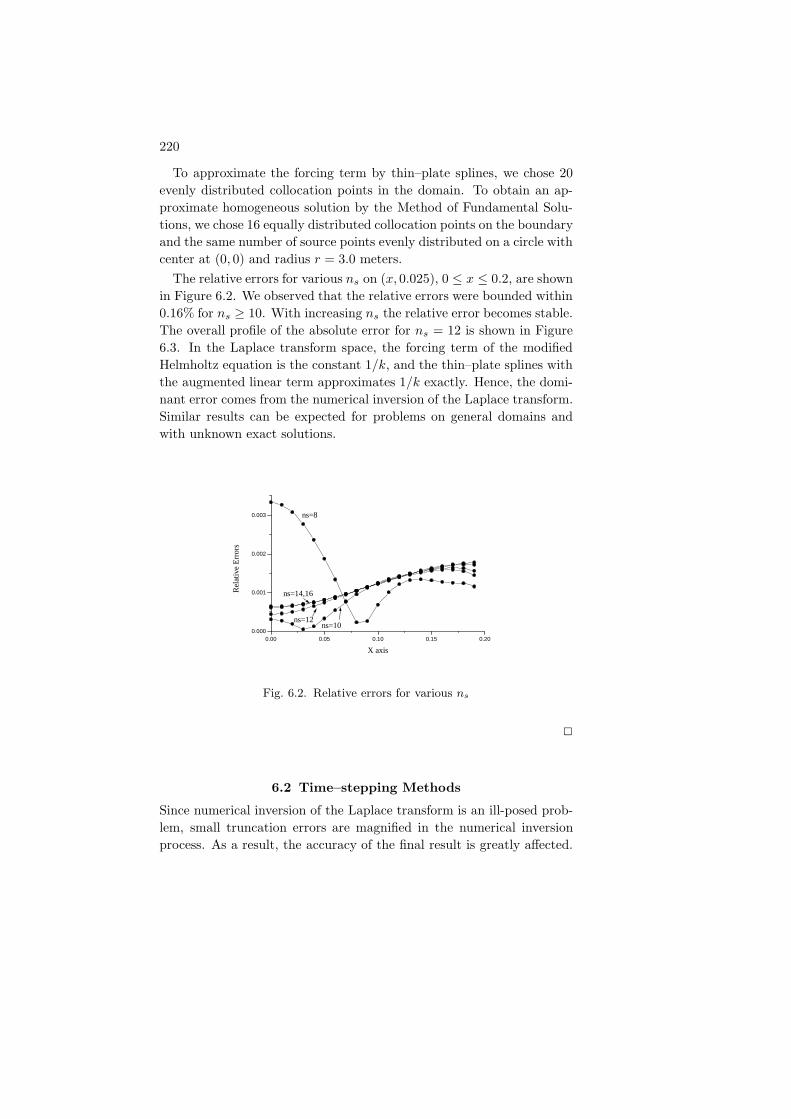
220
To approximate the forcing term by thin–plate splines, we chose 20
evenly distributed collocation points in the domain. To obtain an ap-
proximate homogeneous solution by the Method of Fundamental Solu-
tions, we chose 16 equally distributed collocation points on the boundary
and the same number of source points evenly distributed on a circle with
center at (0, 0) and radius r = 3.0 meters.
The relative errors for various ns on (x, 0.025), 0 ≤ x ≤ 0.2, are shown
in Figure 6.2. We observed that the relative errors were bounded within
0.16% for ns ≥ 10. With increasing ns the relative error becomes stable.
The overall profile of the absolute error for ns = 12 is shown in Figure
6.3. In the Laplace transform space, the forcing term of the modified
Helmholtz equation is the constant 1/k, and the thin–plate splines with
the augmented linear term approximates 1/k exactly. Hence, the domi-
nant error comes from the numerical inversion of the Laplace transform.
Similar results can be expected for problems on general domains and
with unknown exact solutions.
0.00 0.05 0.10 0.15 0.200.000
0.001
0.002
0.003
ns=10ns=12
ns=14,16
ns=8
Rel
ativ
e E
rror
s
X axis
Fig. 6.2. Relative errors for various ns
2
6.2 Time–stepping Methods
Since numerical inversion of the Laplace transform is an ill-posed prob-
lem, small truncation errors are magnified in the numerical inversion
process. As a result, the accuracy of the final result is greatly affected.

Time–Dependent Problems 221
00.2
0.40.6
0.81
0
0.2
0.4
0.6
0.8
10
0.2
0.4
0.6
0.8
1
1.2
1.4
x 10−3
Rel
ativ
e E
rror
Fig. 6.3. Profile of absolute error using ns = 12
In this section, we introduce another popular method for solving time–
dependent problems using a time difference scheme.
The standard Method of Lines takes a spatial discretization of the
domain Ω by points xj ∈ Ω, defines univariate functions uj(t) ≈ u(xj , t)
and transforms the partial differential equation into a system of spatially
coupled ordinary differential equations (ODEs) for these functions.
Then one can use any package for solving large systems of ODEs for
the numerical determination of the uj(t). These methods construct spa-
tial discretizations at various time levels tk determined by the ODE
solver. Radial basis functions can then serve to provide the full spatial
approximations u(x, tk) as interpolants or approximants based on the
data provided by the values uj(tk) ≈ u(xj , tk). Therefore classical line
methods based on radial basis functions reduce to spatial interpolation
or approximation, at each time level, as described in the introductory
sections. A somewhat more sophisticated recent variation expressing
spatial derivatives of radial basis function approximations directly in
terms of the spatial data is due to Fasshauer [Fas04, FF07] and closely
related to pseudospectral methods.
But these methods do not take advantage of fundamental or particular
solutions, as provided by the previous sections. Thus we now describe a
technique which use these to construct approximations at various time
levels, connecting them in time by certain time–stepping methods.

222
6.2.1 Diffusion Equation
A simple thermal diffusion process can be modeled by
1
k
∂u
∂t(x, t) + f(x, t) = ∆u(x, t) (6.2.1)
for all x in a closed spatial domain Ω ⊂ IRd, d = 2, 3 with boundary Γ
and for time t ≥ 0. Here u is the temperature, f is the internal heat
generator, and k is the thermal conductivity. If n is the outward unit
normal vector and q = ∂u/∂n is the heat flux, one can prescribe three
different types of boundary conditions
temperature : u(x, t) = u(x), x ∈ ΓD,
flux :∂u
∂n(x, t) = −q(x), x ∈ ΓN ,
convection :∂u
∂n(x, t) = −h(u(x, t) − u∞), x ∈ ΓC ,
for all t ≥ 0, where h is the heat transfer coefficient and u∞ is the
ambient temperature. The initial condition is given by
u(x, 0) = g(x), x ∈ Ω.
Now the spatial variables are discretized using a combination of the
Method of Fundamental Solutions of Chapter 4 and the Method of Par-
ticular Solutions of Chapter 5, while time is discretized using the finite
difference method.
Generalized trapezoidal methods (θ-methods) are a standard
way of doing this. They are defined as follows [PBW92]. Let the time
step be δt > 0 and define the time mesh tn = nδt, n ≥ 0. For tn−1 ≤t ≤ tn, approximate u(x, t) by
u(x, t) ≃ θu(x, tn) + (1 − θ)u(x, tn−1) (6.2.5)
f(x, t) ≃ θf(x, tn) + (1 − θ)f(x, tn−1) (6.2.6)
so that
∆u(x, t) ≃ θ∆u(x, tn) + (1 − θ)∆u(x, tn−1) (6.2.7)
and
∂u
∂t(x, t) ≃ u(x, tn) − u(x, tn−1)
δt.
Note that the implicit Euler method arises for θ = 1 while the Crank–
Nicholson method has θ = 1/2. Let Γ = ΓD ∪ ΓN ∪ ΓC be a disjoint

Time–Dependent Problems 223
splitting of the spatial boundary. Then (6.2.1) can be discretized as
1
k
un − un−1
δt= θ(∆un − fn) + (1 − θ)(∆un−1 − fn−1) (6.2.8)
where δt is the time step, un = u(x, tn), fn = f(x, tn), and 0 < θ ≤ 1.
In particular, forward differences (θ = 0) cannot be used in the present
formulation. The transformed temperature is defined by
vn = un +(1 − θ)
θun−1. (6.2.9)
Rearranging (6.2.8) gives
∆vn − λ2vn = − 1
θ2kδtun−1 +
(1 − θ)
θfn−1 + fn (6.2.10)
where λ2 = 1/θkδt and u0(x) = g(x). We note that after vn is evaluated,
un can be retrieved from (6.2.9).
Now the diffusion equation (6.2.1) has been transformed into a series
of inhomogeneous modified Helmholtz equations (6.2.10) which can be
solved by a boundary type approach. The most challenging part of
the solution procedure is to effectively obtain an approximate particular
solution.
To solve (6.2.1) at each time step, our standard procedure of splitting
the given problem into a homogeneous solution vnh , and a particular
solution vnp is applied, i.e. vn = vn
h +vnp . The governing equation for the
particular solution is given by
∆vnp − λ2vn
p = − 1
θ2kδtun−1 +
(1 − θ)
θfn−1 + fn. (6.2.11)
As we have indicated in the previous chapters, the particular solution vnp
is not required to satisfy any boundary condition. The governing system
for the homogeneous solution vnh is then given by
∆vnh (x) − λ2vn
h(x) = 0, x ∈ Ω,
vnh(x) = u(x) − vn
p (x), x ∈ ΓD,
qnh(x) = q(x) − qn
p (x), x ∈ ΓN ,
(kqnh + hvn
h) (x) = −kqnp (x) − hvn
p (x) + hu∞(x), x ∈ ΓC .
The right-hand side of (6.2.11) is completely known at each time step
and can be approximated by polyharmonic splines as shown in Chapter
2.

224
Example 6.2.12 Consider the parabolic equation
∂u
∂t(x1, x2, t) = ∆u(x1, x2, t) + f(x1, x2, t)
in the 2D domain [−2, 2]× [−2, 2]. The forcing term is given by
f(x1, x2, t) = sinx1 sinx2(2 sin t+ cos t).
The initial and boundary conditions lead to the solution
u∗(x1, x2, t) = sinx1 sinx2 sin t.
To approximate the forcing term f , we chose 132 interpolation points
in which 32 boundary points were used as the collocation points for the
Method of Fundamental Solutions. We chose the polyharmonic spline
(r4 ln r) of order two from Table 1.3 as the radial basis function. To
evaluate the homogeneous solution using the Method of Fundamental
Solutions, we chose 32 source points on a circle with center at (0, 0) and
radius 8.
To verify the effectiveness of the method, we computed the errors on
a point randomly chosen at (0.889, 0.889). The errors for δt = 0.05 and
δt = 0.025 are shown in Figure 6.4. Similar results were also obtained
at other points. The results are highly accurate for the smaller time
step δt. Increasing the number of interpolation points has only a small
influence on the numerical accuracy.
0 5 10 15 20-0.02
-0.015
-0.01
-0.005
0
0.005
0.01
0.015
0.02
Time (Seconds)
Err
ors
dt=0.05 dt=0.025
Fig. 6.4. Example 6.2.12. Errors for δt = 0.05 and δt = 0.025 at (0.889, 0.889).
To evaluate the global error, we chose 400 evenly distributed points

Time–Dependent Problems 225
on the domain and computed the errors using δt = 0.0125 at t = 10.
The profile of the error over the domain is shown in Figure 6.5, while the
exact solution at t = 10 is displayed in Figure 6.6. The error decreases
linearly with the time step chosen, as shown in Figure 6.7.
−2−1
01
2
−2−1
01
2
−4
−3
−2
−1
0
1
2
3
4
x 10−3
XY
Err
or
Fig. 6.5. Example 6.2.12. Errors at t = 10 using δt = 0.0125.
−2
0
2
−2−1
01
2
−0.8
−0.6
−0.4
−0.2
0
0.2
0.4
0.6
XY
u(x
,y)
Fig. 6.6. Example 6.2.12. Exact solution at t = 10.
2
Example 6.2.13 Consider the diffusion equation (6.2.1) in a 3D cube
0 ≤ x1, x2, x3 ≤ 1 with k = 1 [ICT04]. The boundary conditions are

226
0 0.02 0.04 0.06 0.08 0.1 0.12 0.14 0.16 0.18 0.20
0.01
0.02
0.03
0.04
0.05
0.06
0.07
Time Step
Abs
. Max
. Err
ors
Fig. 6.7. Example 6.2.12. Error in terms of the time discretization.
given by
u(0, x2, x3, t) = 0, u(1, x2, x3, t) = 1, (6.2.14)
∂u
∂n(x1, x2, 0, t) =
∂u
∂n(x1, x2, 1, t) = 0, (6.2.15)
∂u
∂n(x1, 0, x3, t) =
∂u
∂n(x1, 1, x3, t) = 0 (6.2.16)
on the sides of the cube and for positive t. The initial condition is given
by u(x1, x2, x3, 0) = 0 for 0 < x1, x2, x3 < 1. This problem represents
the problem of an insulated unit bar with initial temperature 0 whose
left-hand boundary is isothermal at 0 and whose right hand boundary
is impulsively raised to 1 at time t = 0. The exact solution can be
determined using a separation of variables and is given in [O’N99].
The domain is discretized with 218 source points outside the domain
and 343 collocation points, of which 218 are located on the surface of the
domain while the remaining 125 collocation points are located in the in-
terior of the domain. The radius of the fictitious boundary is 8. In Table
6.1, PS1, PS2 and PS3 denote errors obtained via polyharmonic splines
r2k−1, k = 1, 2, 3, respectively. In general, the results get better with
higher-order polyharmonic splines and reduced time steps, but this is
not always the case. Care must be taken when either reducing the time
step or going to higher-order polyharmonic splines since the higher-order
polyharmonic splines result in worse conditioning of the linear system
associated with the particular solution, while smaller time steps result

Time–Dependent Problems 227
in worse condition of the linear system associated with the homogeneous
solution. In fact, for small time steps, the Euler implicit method (θ = 1)
is more accurate than the Crank–Nicholson method (θ = 1/2) despite
the difference in the local truncation error for the two methods. The cur-
rent results are consistent with findings of Muleshkov et. al. [MGC99]
who showed that significant improvement in accuracy can be obtained
using higher-order polyharmonic splines for elliptic boundary value prob-
lems. Further, they observed limited improvement for time–dependent
problems, presumably because the dominating error was caused by the
time-stepping scheme. 2
θ ∆t PS1 PS2 PS3
0.01 1.00E − 2 2.83E − 3 1.38E − 20.005 1.57E − 2 2.77E − 3 2.40E − 3
0.5 0.002 2.92E − 2 2.47E − 3 1.96E − 30.001 4.56E − 2 2.50E − 3 overflow
0.01 1.73E − 2 1.39E − 2 1.38E − 20.005 1.35E − 2 7.20E − 3 7.07E − 3
1 0.002 1.84E − 2 3.31E − 3 3.02E − 30.001 2.86E − 2 2.26E − 3 1.76E − 3
Table 6.1. Example 6.2.13. Absolute maximum errors at t = 1 using
polyharmonic splines.
6.2.2 Convection-Diffusion Problems
The standard two-dimensional convection-diffusion equation is of
the form
1
k
∂u
∂t+ wx
∂u
∂x+ wy
∂u
∂y+ f = ∆u, (6.2.17)
where wx and wy are the components of a variable velocity vector field
and f is the source term. The solution to this problem is formulated in
the same manner as before by explicitly combining the convection and
source terms, i.e.
F = wx∂u
∂x+ wy
∂u
∂y+ f.
228
In this way, (6.2.17) can be solved like (6.2.1) in the diffusion case.
Consequently,
∆vnp − λ2vn
p = − 1
θ2kδtun−1 +
(1 − θ)
θFn−1 + Fn
is another inhomogeneous modified Helmholtz equation which can be
solved similar to the case of diffusion equations as before.
6.2.3 Semi-nonlinear Diffusion Equation
If the convection term in (6.2.17) is replaced by a general nonlinear term
of the form f(x, t, u,∇u), the method given above can be modified to
solve the nonlinear diffusion equation
1
k
∂u
∂t(x, t) + f(x, t,∇u, u) = ∆u(x, t). (6.2.18)
Again, u(x, t) can be approximated by (6.2.5) using the θ–method. In
the next example, we choose θ = 1 Similar to the derivation of (6.2.10),
we can reformulate (6.2.18) as
∆vn − λ2vn = − 1
θ2kδtun−1 + fn−1,
where vn is defined in (6.2.9). Interestingly, this scheme requires no
spatial iteration. This is in sharp contrast to the steady state case
∂u/∂t = 0 [Che95].
Example 6.2.19 We first consider the two-dimensional Fisher equa-
tion [Bri86, Lan99]
∂u
∂t= ∆u+ κu(1 − u) in Ω × (0, T ], κ ≥ 0, (6.2.20)
with initial and boundary conditions
u(x, 0) = J0
(c
√x2
1
9+ x2
2
)in Ω, (6.2.21)
u(x, t) = 0 on Γ × (0, T ], (6.2.22)
where J0 is the first kind Bessel function of order zero, c ≃ 2.4048 is
the first zero of J0 and x = (x1, x2). The physical domain is an ellipse
Ω ∪ Γ = (x1, x2) : x21/9 + x2
2 ≤ 1.The existence and uniqueness of a solution to (6.2.20)-(6.2.22) was
proven by Britton [Bri86]. Furthermore, there exists a critical value
δ∗ > 0 such that the zero solution is a stable steady state for κ < δ∗,
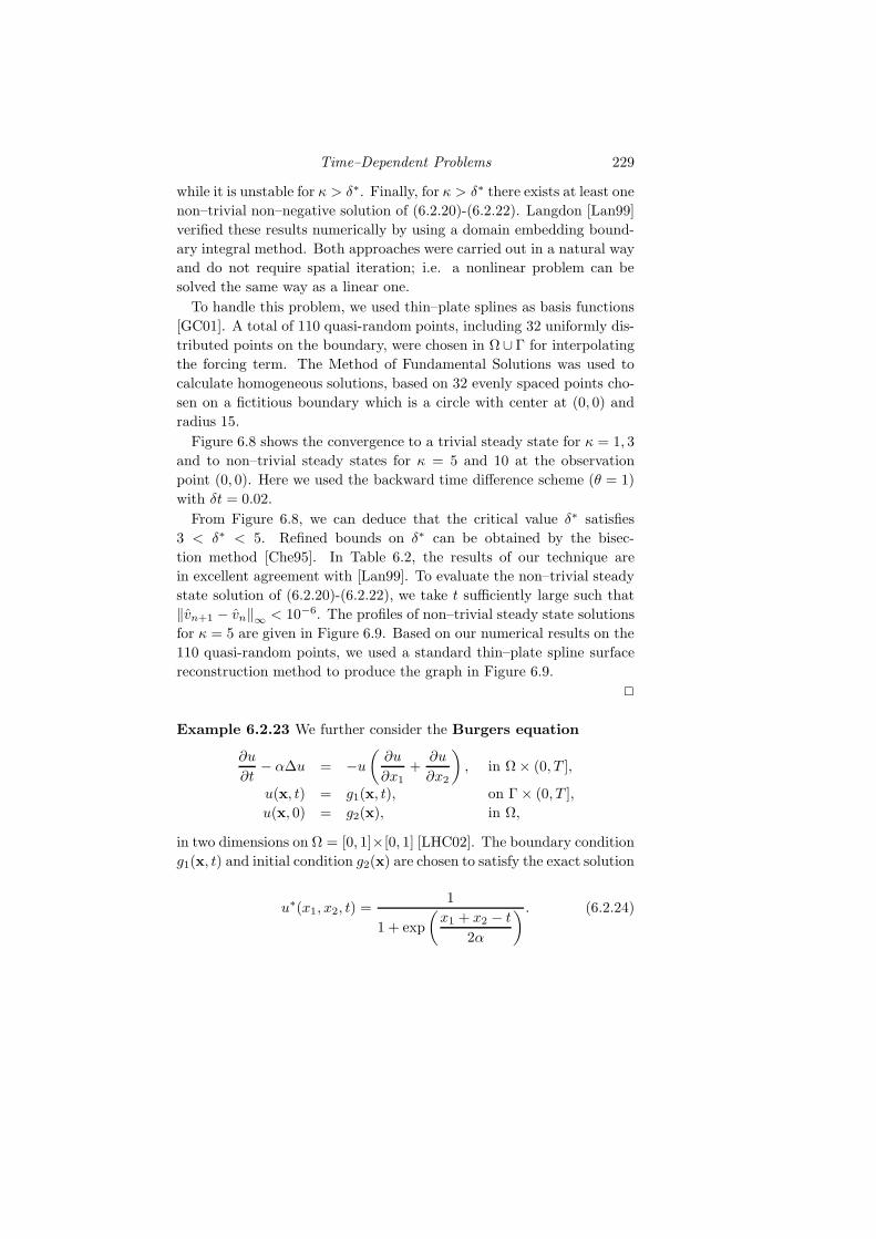
Time–Dependent Problems 229
while it is unstable for κ > δ∗. Finally, for κ > δ∗ there exists at least one
non–trivial non–negative solution of (6.2.20)-(6.2.22). Langdon [Lan99]
verified these results numerically by using a domain embedding bound-
ary integral method. Both approaches were carried out in a natural way
and do not require spatial iteration; i.e. a nonlinear problem can be
solved the same way as a linear one.
To handle this problem, we used thin–plate splines as basis functions
[GC01]. A total of 110 quasi-random points, including 32 uniformly dis-
tributed points on the boundary, were chosen in Ω ∪ Γ for interpolating
the forcing term. The Method of Fundamental Solutions was used to
calculate homogeneous solutions, based on 32 evenly spaced points cho-
sen on a fictitious boundary which is a circle with center at (0, 0) and
radius 15.
Figure 6.8 shows the convergence to a trivial steady state for κ = 1, 3
and to non–trivial steady states for κ = 5 and 10 at the observation
point (0, 0). Here we used the backward time difference scheme (θ = 1)
with δt = 0.02.
From Figure 6.8, we can deduce that the critical value δ∗ satisfies
3 < δ∗ < 5. Refined bounds on δ∗ can be obtained by the bisec-
tion method [Che95]. In Table 6.2, the results of our technique are
in excellent agreement with [Lan99]. To evaluate the non–trivial steady
state solution of (6.2.20)-(6.2.22), we take t sufficiently large such that
‖vn+1 − vn‖∞ < 10−6. The profiles of non–trivial steady state solutions
for κ = 5 are given in Figure 6.9. Based on our numerical results on the
110 quasi-random points, we used a standard thin–plate spline surface
reconstruction method to produce the graph in Figure 6.9.
2
Example 6.2.23 We further consider the Burgers equation
∂u
∂t− α∆u = −u
(∂u
∂x1+
∂u
∂x2
), in Ω × (0, T ],
u(x, t) = g1(x, t), on Γ × (0, T ],
u(x, 0) = g2(x), in Ω,
in two dimensions on Ω = [0, 1]×[0, 1] [LHC02]. The boundary condition
g1(x, t) and initial condition g2(x) are chosen to satisfy the exact solution
u∗(x1, x2, t) =1
1 + exp
(x1 + x2 − t
2α
) . (6.2.24)

230
u(0, 0) (Langdon) u(0, 0) (MFS-MPS)
Time k = 1 k = 5 k = 10 k = 1 k = 5 k = 10
0.5 3.46E-1 6.14E-1 9.04E-1 3.45E-1 6.15E-1 9.03E-1
1.0 1.41E-1 5.48E-1 8.67E-1 1.40E-1 5.49E-1 8.69E-1
1.5 5.96E-2 5.22E-1 8.50E-1 5.89E-2 5.23E-1 8.54E-1
2.0 2.54E-2 5.10E-1 8.42E-1 2.50E-2 5.10E-1 8.47E-1
2.5 1.08E-2 5.04E-1 8.37E-1 1.06E-2 5.04E-1 8.43E-1
3.0 4.66E-3 5.01E-1 8.34E-1 4.55E-3 5.01E-1 8.40E-1
3.5 1.99E-3 5.00E-1 8.32E-1 1.94E-3 5.00E-1 8.39E-1
4.0 8.57E-4 4.99E-1 8.31E-1 8.31E-4 4.99E-1 8.38E-1
4.5 3.67E-4 4.99E-1 8.30E-1 3.55E-4 4.99E-1 8.38E-1
5.0 1.57E-4 4.99E-1 8.29E-1 1.51E-4 4.99E-1 8.37E-1
Table 6.2. Example 6.2.19. Comparison of u(0, 0) using different
methods.
The solution in (6.2.24) is a wave front moving along the line x1 +x2− t.The profile for α = 0.05 and t = 1.0 is shown in Figure 6.10. The
numerical solutions were obtained by choosing the fully implicit time
stepping scheme θ = 1 and the time step δt = 0.01. From (6.2.9)-
(6.2.10), we have
∆un − 1
αδtun = − 1
αδtun−1 +
1
αun−1
(∂un−1
∂x1+∂un−1
∂x2
).
The spatial domain Ω is discretized by 19×19 uniform grid points inside
Ω. Third order polyharmonic splines (r6 ln r) are chosen to approximate
the forcing term. For the implementation of the Method of Fundamental
Solutions, 32 points were evenly distributed on the boundary Γ. For the
initial step, u0 = g2(x) and
∂u0
∂xi=∂g2∂xi
, i = 1, 2,
are used. For the time step n ≥ 1, we have
∂un
∂xi=∂un
h
∂xi+∂un
p
∂xi, i = 1, 2,
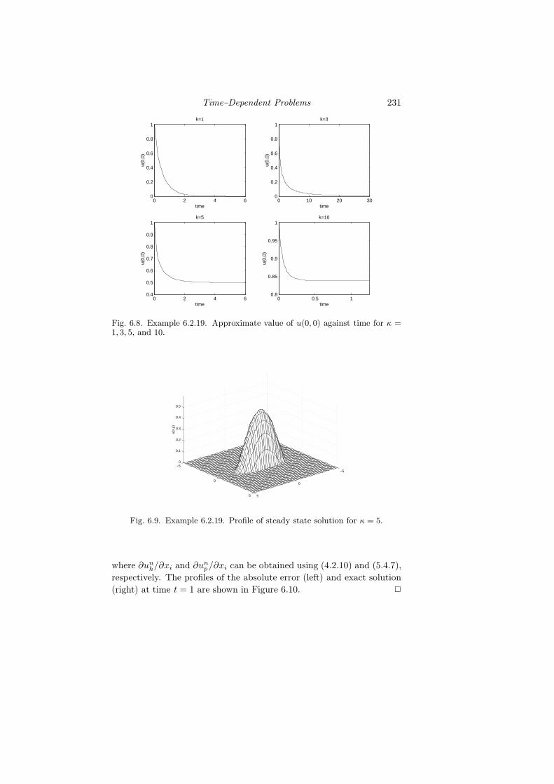
Time–Dependent Problems 231
0 2 4 60
0.2
0.4
0.6
0.8
1
time
u(0,
0)
k=1
0 10 20 300
0.2
0.4
0.6
0.8
1
time
u(0,
0)
k=3
0 2 4 60.4
0.5
0.6
0.7
0.8
0.9
1
time
u(0,
0)
k=5
0 0.5 10.8
0.85
0.9
0.95
1k=10
time
u(0,
0)
Fig. 6.8. Example 6.2.19. Approximate value of u(0, 0) against time for κ =1, 3, 5, and 10.
−5
0
5
−5
0
5
0
0.1
0.2
0.3
0.4
0.5
u(x,
y)
Fig. 6.9. Example 6.2.19. Profile of steady state solution for κ = 5.
where ∂unh/∂xi and ∂un
p/∂xi can be obtained using (4.2.10) and (5.4.7),
respectively. The profiles of the absolute error (left) and exact solution
(right) at time t = 1 are shown in Figure 6.10. 2

232
0
0.01
0.02
0.03
0.04
00.25
0.50.75
1X
00.2
0.40.6
0.81
Y
Y
Z
X
Error4.6243E-024.3160E-024.0077E-023.6994E-023.3912E-023.0829E-022.7746E-022.4663E-022.1580E-021.8497E-021.5414E-021.2331E-029.2486E-036.1657E-033.0829E-03
00.2
0.40.6
0.81 0
0.20.4
0.60.8
1
0
0.1
0.2
0.3
0.4
0.5
0.6
0.7
0.8
0.9
1
YX
Z
Fig. 6.10. Error and solution profiles at t = 1.
6.3 Operator-Splitting Methods
Consider the nonlinear diffusion–reaction equation
∂u
∂t= ∆u+ f(u) on Ω (6.3.1)
with boundary conditions
u(x, t) = u0(x, t), on ΓD,∂u
∂n(x, t) = 0, on ΓN ,
where Γ = ΓD ∪ ΓN denotes the boundary of Ω, and f is a nonlinear
forcing function. The operator splitting method is a procedure to
separate the elliptic operator from the nonlinear forcing term, followed
by an approach similar to the alternating direction implicit (ADI) pro-
cedure proposed by Peaceman and Rachford [PR55]. Balakrishnan et.
al. [BSR02] generalized the procedure in the context of the Method of
Fundamental Solutions and Radial Basis Functions.
In general, a time–dependent problem can be written as
∂u
∂t= L1 + L2 + · · ·Ln
via a sum of n operators L1, L2, · · · , Ln. In (6.3.1), we have the following
expressions
L1 = f(u) (6.3.2)
L2 = ∆u. (6.3.3)
To discretize ∂u/∂t, a two-time-step finite difference scheme can be used.

Time–Dependent Problems 233
More specifically, the non–linear forcing term in (6.3.2) is evaluated ex-
plicitly at each half time step and the resulting solution is then used for
an implicit solution of the Laplacian term in (6.3.3). For the first half
step, we can use the second order explicit Adams-Bashforth scheme
and obtain
un+1/2 − un
δt=
3
2f(un) − 1
2f(un−1). (6.3.4)
The solution un+1/2 from (6.3.4) is then used in the next half step, which
can be discretized implicitly using the second order Adams-Moulton
scheme as
un+1 − un+1/2
δt=
1
2(∆un+1 + ∆un). (6.3.5)
We observe that the non–linear term in (6.3.4) is evaluated explicitly
without any spatial iteration. We also note that the evaluation of the
Laplace operator for the previous step in (6.3.5) will add some error
to the one induced by the time difference scheme. To circumvent this
difficulty, the dependent variable in (6.3.5) is transformed to u∗ via
u∗ ≡ un + un+1
2. (6.3.6)
Then
∆u∗ − 2u∗
δt= −(
3
2fn − 1
2fn−1) − 2un
δt(6.3.7)
can be achieved by using (6.3.4)-(6.3.6) and some algebraic manipula-
tions. Again, we observe that (6.3.7) is a modified Helmholtz equation,
solvable by the procedures of the previous chapters. Fortunately, at each
time step the non–homogeneous term is explicitly known. Furthermore,
u∗ can be computed at each time step by the solution of (6.3.7). The val-
ues of un+1 are then extracted from the computed values of u∗ through
(6.3.6). We remark that the whole solution process needs the function
values at the current and previous time step. Hence, the method itself
is not self-starting, and an extrapolated explicit forward Euler method
is used for simplicity for the first time step to initiate the time stepping.
For numerical examples and further details, we refer the reader to the
work of Balakrishnan et. al. [BSR02].
6.3.1 Stokes Flow
The Stokes flow problem is a simplification of the Navier-Stokes
problem, in which the nonlinear convective terms are very small and

234
can be neglected. For the solution of Stokes flows using the velocity–
vorticity formulation, the governing equations can be written as a
system of diffusion-type and Poisson–type equations for the components
of the vorticity and velocity field, respectively. This means
∂ω
∂t= ∆ω
∆u = −∇× ω
in Ω (6.3.8)
u = U on Γ (6.3.9)
where u is the velocity vector, ω the vorticity vector, U the given bound-
ary velocity and Ω, Γ denote the domain and its boundary, respectively.
Furthermore, the vorticity vector ω can be expressed as
ω = ∇× u.
One of the advantages of this formulation is the separation of the kine-
matic and kinetic aspects of the fluid flow.
The general numerical procedure for solving (6.3.8) and (6.3.9) can be
described as follows:
(i) Set the initial value to be zero:
u0(x) = (u01(x), u0
2(x), u03(x)) = (0, 0, 0)
ω0(x) = (ω01(x), ω0
2(x), ω03(x)) = (0, 0, 0)
and un = u(x, nδt), ωn = ω(x, nδt).
(ii) Solve ∆un+1 = 0 with the given boundary velocity condition
u = U (Laplace equation).
(iii) Obtain the vorticity on the boundary using ωn+1 = ∇× un+1.
(iv) Solve the diffusion equation in (6.3.8) for ωn+1 with the boundary
condition from step (iii).
(v) Solve the velocity equation in (6.3.9) with the given boundary
condition (Poisson equation) for un+1. The forcing term is the
derivative of the vorticity components obtained from step (iv).
(vi) Repeat step (iii)-(v) until the solutions are convergent.
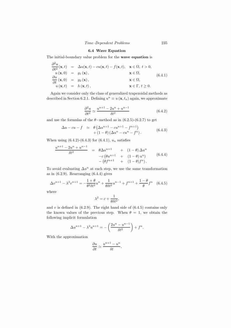
Time–Dependent Problems 235
6.4 Wave Equation
The initial-boundary value problem for the wave equation is
∂2u
∂t2(x, t) = ∆u(x, t) − cu(x, t) − f(x, t), x ∈ Ω, t > 0,
u (x, 0) = g1 (x) , x ∈ Ω,∂u
∂t(x, 0) = g2 (x) , x ∈ Ω,
u (x, t) = h (x, t) , x ∈ Γ, t ≥ 0.
(6.4.1)
Again we consider only the class of generalized trapezoidal methods as
described in Section 6.2.1. Defining un ≡ u (x, tn) again, we approximate
∂2u
∂t2≃ un+1 − 2un + un−1
δt2(6.4.2)
and use the formulas of the θ−method as in (6.2.5)-(6.2.7) to get
∆u− cu− f ≃ θ(∆un+1 − cun+1 − fn+1
)
+ (1 − θ) (∆un − cun − fn) .(6.4.3)
When using (6.4.2)-(6.4.3) for (6.4.1), un satisfies
un+1 − 2un + un−1
δt2= θ∆un+1 + (1 − θ) ∆un
−c(θun+1 + (1 − θ) un)
−(θfn+1 + (1 − θ)fn) .
(6.4.4)
To avoid evaluating ∆un at each step, we use the same transformation
as in (6.2.9). Rearranging (6.4.4) gives
∆vn+1 − λ2vn+1 = −1 + θ
θ2δt2un +
1
θδt2un−1 + fn+1 +
1 − θ
θfn (6.4.5)
where
λ2 = c+1
θδt2,
and v is defined in (6.2.9). The right hand side of (6.4.5) contains only
the known values of the previous step. When θ = 1, we obtain the
following implicit formulation
∆un+1 − λ2un+1 = −(
2un − un−1
δt2
)+ fn.
With the approximation
∂u
∂t≃ un+1 − un
δt,

236
we get the initial conditions
u0 (x) = g1 (x) , x ∈ Ω ∪ Γ, (6.4.6)
u1 (x) = g1 (x) + δtg2 (x) , x ∈ Ω ∪ Γ, (6.4.7)
and boundary conditions
un+1 (x) = hn+1 (x) , x ∈ Γ.
Note that (6.4.5) is again a modified Helmholtz equation. Hence at each
time step un satisfies a boundary-value problem for a modified Helmholtz
equation. The solution procedure is quite similar to the diffusion equa-
tion using the approach described in Section 6.2.1.
Example 6.4.8 Consider the wave equation
∂2u
∂t2(x, t) = ∆u(x, t), x ∈ Ω, t > 0
u (x, 0) = sin2 (πx1) sin(πx2), x ∈ Ω,∂u
∂t(x, 0) = 0, x ∈ Ω,
u (x, t) = 0, x ∈ Γ,
where x = (x1, x2), Ω∪Γ = [0, 1]× [0, 1]. The exact solution is given by
u(x1, x2, t) =−8
π
∞∑
n=1,3,5,···
cos(πt√n2 + 1
)
n(n2 − 4)sinnπx1 sinπx2.
To evaluate the particular solution at each time step, we chose 121 evenly
distributed grid points on Ω ∪ Γ. As our radial basis function we chose
polyharmonic splines (1.3) of order two, i.e. φ(r) = r4 ln r. To solve the
homogeneous equation, we chose 32 collocation points on the boundary
and 32 source points on the fictitious circle with center at (0.5, 0.5) and
radius r = 2. For the time-stepping scheme, we chose the fully implicit
method with θ = 1. Figure 6.11 shows both the profiles of the exact and
the approximate solution at (0.5, 0.5) over the time interval 0 ≤ t ≤ 6.
We have noticed that the larger errors occur near turning points of each
cycle. The accuracy when using the smaller time step (dt = 0.001) is far
better than the larger time step (dt = 0.01). The profiles of the exact
solution and the error u − un on the whole domain at t = 2.8, 6 using
δt = 0.001 are shown in Figures 6.12-6.13. 2

Time–Dependent Problems 237
0 1 2 3 4 5 6
−1
−0.8
−0.6
−0.4
−0.2
0
0.2
0.4
0.6
0.8
1
dt = 0.01
Time
Err
or
Approx.Exact
0 1 2 3 4 5 6
−1
−0.8
−0.6
−0.4
−0.2
0
0.2
0.4
0.6
0.8
1
dt = 0.001
Time
Err
or
Exact Approx.
Fig. 6.11. Example 6.4.8: un(0.5, 0.5) for δt = 0.01 and 0.001
00.2
0.40.6
0.81
00.2
0.40.6
0.81
0
0.1
0.2
0.3
0.4
0.5
0.6
0.7
0.8
X
T = 2.8
Y
u(x
,y)
00.2
0.40.6
0.81
0
0.5
1
−0.01
0
0.01
0.02
0.03
0.04
0.05
X
T = 2.8
Y
Err
or
Fig. 6.12. Example 6.4.8: The profiles of un (left) and errors (right) at t = 2.8using δt = 0.001
Example 6.4.9 Consider the wave equation
∂2u
∂t2(x, t) = ∆u(x, t) + f(x, t), x ∈ Ω, t > 0,
u (x, 0) = x1(1 − x1)x2(1 − x2), x ∈ Ω,∂u
∂t(x, 0) = 0, x ∈ Ω,
u (x, t) = x1(1 − x1)x2(1 − x2) cos(t), x ∈ Γ,
00.20.40.60.81
0
0.5
1
−0.15
−0.1
−0.05
0
0.05
0.1
0.15
0.2
X
T = 6
Y
u(x
,y)
00.20.40.60.81
0
0.5
1
−0.04
−0.02
0
0.02
0.04
0.06
X
T = 6
Y
Err
or
Fig. 6.13. The profiles of un (left) and errors (right) at t = 6 using δt = 0.001.

238
where
f(x, t) = (2x1(1 − x1) + 2x2(1 − x2) − x1(1 − x1)x2(1 − x2)) cos(t)
and x = (x1, x2), Ω ∪ Γ = [0, 1] × [0, 1]. The exact solution is
u∗(x1, x2, t) = x1(1 − x1)x2(1 − x2) cos(t).
The number of collocation points, the radial basis function, and the
time-stepping scheme are like in the previous example. For the time
step we chose δt = 0.05. From (6.4.7), the initial condition ∂u∂t = 0
implies u0 = u1. The profiles of u(x1, x2) and the errors at t = 1, 3, 5
are shown in Figures 6.14 to 6.16. The solution u is vibrating up and
down. In Figure 6.17, we show the errors of u(0.5, 0.5, t) for 0 ≤ t ≤ 20
using time steps δt = 0.01, and 0.025. This shows that the error is
oscillating, but stable. However, the smaller time step did not improve
the error as much as in the last example and for the diffusion equation
in Example 6.2.12. We offer no further explanation here as no error
analysis is available. It is possible that the source term f(x, t) cancels
the damping effect as shown in the previous example.
0
0.2
0.4
0.6
0.8
1
00.2
0.40.6
0.81
0
0.005
0.01
0.015
0.02
0.025
0.03
0.035
X
T = 1
Y
u(x
,y)
0
0.2
0.4
0.6
0.8
1
00.2
0.40.6
0.81
0
1
2
3
4
5
x 10−4
X
T = 1
Y
Err
or
Fig. 6.14. Example 6.4.9: The profiles of un (left) and errors (right) at t = 1.
2
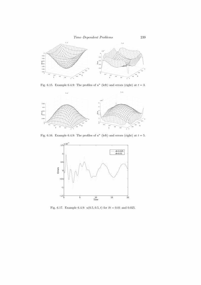
Time–Dependent Problems 239
0
0.2
0.4
0.6
0.8
1
00.2
0.40.6
0.81
−0.07
−0.06
−0.05
−0.04
−0.03
−0.02
−0.01
0
X
T = 3
Y
u(x
,y)
0
0.2
0.4
0.6
0.8
1
00.2
0.40.6
0.81
−1
−0.8
−0.6
−0.4
−0.2
0
x 10−3
X
T = 3
Y
Err
or
Fig. 6.15. Example 6.4.9: The profiles of un (left) and errors (right) at t = 3.
0
0.2
0.4
0.6
0.8
1
00.2
0.40.6
0.81
0
0.005
0.01
0.015
0.02
0.025
X
T = 5
Y
u(x
,y)
0
0.2
0.4
0.6
0.8
1
00.2
0.40.6
0.81
0
1
2
3
4
5
x 10−4
X
T = 5
Y
Err
or
Fig. 6.16. Example 6.4.9: The profiles of un (left) and errors (right) at t = 5.
0 5 10 15 20−1.5
−1
−0.5
0
0.5
1
1.5x 10
−3
Time
Err
ors
dt=0.025dt=0.01
Fig. 6.17. Example 6.4.9: u(0.5, 0.5, t) for δt = 0.01 and 0.025.

References
Bibliography
[AA05] C.J.S. Alves and P.R.S. Antunes, The method of fundamental solutionsapplied to the calculation of eigenfrequencies and eigenmodes of 2d simplyconnected shapes, Compters, Materials, and Continua (2005), 251–266.
[ABW06] R. Ahrem, A. Beckert, and H. Wendland, A meshless spatial cou-pling scheme for large-scale fluid-structure-interaction problems, Com-puter Modeling in Engineering and Sciences 12 (2006), 121–136.
[AC01] C.J.S. Alves and C.S. Chen, The MFS method adapted for a nonho-mogeneous equation, Advances in Computational Engineering & Sciences(S.N. Atluri, T. Nishioka, and M. Kikuchi, eds.), Tech Science Press, LosAngeles, CD Rom, # 135, 2001.
[AC05] , Approximating functions and solutions of non homogeneouspartial differential equations using the method of fundamental solutions,Advances in Computational Mathematics (2005), 125–142.
[ADR94] N. Arad, N. Dyn, and D. Reisfeld, Image warping by radial basisfunctions: applications to facial expressions, Graphical Models and ImageProcessing 56 (1994), 161–172.
[AS65] M. Abramowitz and I.A. Stegun, Handbook of Mathematical Functions,Dover, New York, 1965.
[Atk85] K.E. Atkinson, The numerical evaluation of particular solutions forPoisson’s equation, IMA Journal of Numerical Analysis 5 (1985), 319–338.
[AZ98a] S.N. Atluri and T.-L. Zhu, A new meshless local Petrov-Galerkin(MLPG) approach in Computational mechanics, Computational Mechan-ics 22 (1998), 117–127.
[AZ98b] , A new meshless local Petrov-Galerkin (MLPG) approach tononlinear problems in Computer modeling and simulation, ComputerModeling and Simulation in Engineering 3 (1998), 187–196.
[AZ00] , The meshless local Petrov-Galerkin (MLPG) approach for solv-ing problems in elasto-statics, Computational Mechanics 25 (2000), 169–179.
[Bax02] B.J.C. Baxter, Preconditioned conjugate gradients, radial basis func-tions, and Toeplitz matrices, Comput. Math. Appl. 43 (2002), 305–318.
[BC00] R.K. Beatson and E. Chacko, Fast evaluation of radial basis functions:A multivariate momentary evaluation scheme, Curve and Surface Fit-
240

References 241
ting: Saint-Malo 1999 (A. Cohen, C. Rabut, and L.L. Schumaker, eds.),Vanderbilt University Press, 2000, pp. 37–46.
[BCM99] R.K. Beatson, J.B. Cherrie, and C.T. Mouat, Fast fitting of radialbasis functions: Methods based on preconditioned GMRES iteration, Adv.Comput. Math. 11 (1999), 253–270.
[BCR00] R.K. Beatson, J.B. Cherrie, and D.L. Ragozin, Polyharmonic splines
in IRd: Tools for fast evaluation, Curve and Surface Fitting: Saint-Malo1999 (A. Cohen, C. Rabut, and L.L. Schumaker, eds.), Vanderbilt Uni-versity Press, 2000, pp. 47–56.
[BG97] R.K. Beatson and L. Greengard, A short course on fast multipole meth-ods, Wavelets, Multilevel Methods and Elliptic PDEs (M. Ainsworth,J. Levesley, W. Light, and M. Marletta, eds.), Oxford University Press,1997, pp. 1–37.
[BGP96] R.K. Beatson, G. Goodsell, and M.J.D. Powell, On multigrid tech-niques for thin plate spline interpolation in two dimensions, The math-ematics of numerical analysis, Lectures in Appl. Math., vol. 32, Amer.Math. Soc., Providence, RI, 1996, pp. 77–97.
[BK05] M. Botsch and L. Kobbelt, Real-time shape editing using radial basisfunctions, Computer Graphics Forum, vol. 24, 2005, pp. 611–621.
[BKO+96] T. Belytschko, Y. Krongauz, D.J. Organ, M. Fleming, and P. Krysl,Meshless methods: an overview and recent developments, ComputerMethods in Applied Mechanics and Engineering, special issue 139 (1996),3–47.
[BL97] R.K. Beatson and W.A. Light, Fast evaluation of radial basis functions:Methods for two–dimensional polyharmonic splines, IMA Journal of Nu-merical Analysis 17 (1997), 343–372.
[BLB00] R.K. Beatson, W.A. Light, and S. Billings, Fast solution of the radialbasis function interpolation equations: domain decomposition methods,SIAM J. Sci. Comput. 22 (2000), no. 5, 1717–1740.
[BLKL05] D. Brown, L. Ling, E.J. Kansa, and J. Levesley, On approximatecardinal preconditioning methods for solving PDEs with radial basis func-tions, Engineering Analysis with Boundary Elements 19 (2005), 343–353.
[BM97] I. Babuska and J.M. Melenk, The Partition of Unity Method, Int. J.Numer. Meths. Eng. 40 (1997), 727–758.
[BN92] R.K. Beatson and G.N. Newsam, Fast evaluation of radial basis func-tions. I, Comput. Math. Appl. 24 (1992), no. 12, 7–19, Advances in thetheory and applications of radial basis functions.
[Bog85] A. Bogomolny, Fundamental solutions method for elliptic boundaryvalue problems, SIAM J. Numer. Anal. 22 (1985), 644–669.
[Bra01] D. Braess, Finite elements. Theory, fast solvers and applications insolid mechanics, Cambridge University Press, 2001.
[Bri86] N.F. Britton, Reaction-diffusion equations and their applications to Bi-ology, Academic Press, 1986.
[BS87] C.V. Bellos and J.G. Sakkas, 1-D dam-break flood-wave propagation ondry bed, Journal of Hydraulic Engineering 113 (1987), 1510–1524.
[BS02] S.C. Brenner and L.R. Scott, The mathematical theory of finite elementmethods, second edition, Springer, 2002.
[BSR02] K. Balakrishnan, R. Sureshkumar, and P.A. Ramachandran, An oper-ator splitting-RBF method for the solution of transient nonlinear Poissonproblems, Computers and Mathematics with Applications 43 (2002), 289–304.

242 References
[Buh88] M.D. Buhmann, Convergence of univariate quasi-interpolation usingmultiquadrics, IMA J. Numer. Anal. 8 (1988), 365–383.
[Buh90] , Multivariate cardinal interpolation with radial–basis functions,Constr. Approx. 6 (1990), 225–255.
[Buh98] , Radial functions on compact support, Proceedings of the Ed-inburgh Mathematical Society 41 (1998), 33–46.
[Buh03] , Radial basis functions, theory and implementations, Cam-bridge University Press, 2003.
[Bur40] J.M. Burgers, Application of a model system to illustrate some pointsof the statistical theory of free turbulence, Proc. Acad. Sci. Amsterdam43 (1940), 2–12.
[CAB92] A.H.-D. Cheng, Y. Abousleiman, and T. Badmus, A Laplace trans-form BEM for axisymmetric diffusion utilizing pre-tabulated Greeen’sfunction, Eng. Anal. Boundary Elements 9 (1992), 39–46.
[CAO94] A.H.-D. Cheng, H. Ahtes, and N. Ortner, Fundamental solutions ofproduct of Helmholtz and polyharmonic operators, Eng. Anal. BoundaryElements 14 (1994), 187–191.
[CBC+01] J.C. Carr, R.K. Beatson, J.B. Cherrie, T.J. Mitchell, W.R. Fright,B.C. McCallum, and T.R. Evans, Reconstruction and representation of3D objects with radial basis functions, Computer Graphics Proceedings,Addison Wesley, 2001, pp. 67–76.
[CBN02] J.B. Cherrie, R.K. Beatson, and G.N. Newsam, Fast evaluation of ra-dial basis functions: Methods for generalised multiquadrics in IRn, SIAMJ. Sci. Comput. 23 (2002), 1272–1310.
[CBP99] C.S. Chen, C.A. Brebbia, and H. Power, Dual reciprocity method usingcompactly supported radial basis functions, Comm. Num. Meth. Eng. 15(1999), 137–150.
[CC05a] A.H.-D. Cheng and J.J.S.P. Cabral, Direct solution of certain ill-posed boundary value problems by collocation method, Boundary ElementsXXVII (A. Kassab, C.A. Brebbia, E. Divo, and D. Poljak, eds.), 2005,pp. 35–44.
[CC05b] , Direct solution of ill-posed boundary value problems by radialbasis function collocation method, Internat. J. Numer. Methods Engrg. 64(2005), no. 1, 45–64.
[CCG06] H.A. Cho, C.S. Chen, and M.A. Golberg, Some comments on miti-gating the ill-conditioning of the method of fundamental solutions, Engi-neering Analysis with Boundary Elements 30 (2006), 405–410.
[CFB97] J.C. Carr, W.R. Fright, and R.K. Beatson, Surface interpolation withradial basis functions for medical imaging, IEEE Transactions on MedicalImaging 16 (1997), 96–107.
[CGGC02] C.S. Chen, M.A. Golberg, M. Ganesh, and A.H.-D. Cheng, Multi-level compact radial functions based computational schemes for some el-liptic problems, Computers and Mathematics with Application 43 (2002),359–378.
[CGML04] H.A. Cho, M.A. Golberg, A.S. Muleshkov, and X. Li, Trefftz meth-ods for time dependent partial differential equations, Computers, Materi-als, and Continua 1 (2004), 1–38.
[CGR98] C.S. Chen, M.A. Golberg, and Y.F. Rashed, A mesh free method forlinear diffusion equations, Numerical Heat Transfer, Part B 33 (1998),469–486.
[CGS03] C.S. Chen, M.A. Golberg, and R. Schaback, Recent developments of

References 243
the dual reciprocity method using compactly supported radial basis func-tions, Transformation of Domain Effects to the Boundary (Y.F. Rashed,ed.), WIT Press, 2003, pp. 183–225.
[CH03] W. Chen and Y.C. Hon, Numerical convergence of boundary knotmethod in the analysis of Helmholtz, modified Helmholtz, and convection-diffusion problems, Computer Methods Appl. Mech. Engng. 192 (2003),1859–1875.
[Cha67] A.J. Chapman, Heat transfer, Macmillan, New York, 1967.[Che87] R.S.C. Cheng, Delta-trigonometric and spline methods using the single-
layer potential representation, Ph.D. thesis, University of Maryland, 1987.[Che95] C.S. Chen, The method of fundamental solutions for non-linear thermal
explosions, Comm. Numer. Methods Engrg. 11 (1995), no. 8, 675–681.[Che02] W. Chen, Symmetric boundary knot method, Engineering Analysis with
Boundary Elements 26 (2002), 489–494.[CJ59] H.S. Carslaw and J.C. Jaeger, Conduction of heat in solids, Oxford
University Press, London, 1959.[CLG94] A.H.-D. Cheng, O. Lafe, and S. Grilli, Dual reciprocity BEM based on
global interpolation functions, Eng. Anal. Boundary Elements 13 (1994),303–311.
[CLH07] C.S. Chen, Sungwook Lee, and C.-S. Huang, The method of partic-ular solutions using chebyshev polynomial based functions, InternationalJournal of Computational Methods 4(1) (2007), 15–32.
[CM78] I. Christie and A.R. Mitchell, Upwinding of high order Galerkin meth-ods in conduction-convection problems, Int. J. Num. Meth. Eng. 12(1978), 1764–1771.
[CMC99] C.S. Chen, M.D. Marcozzi, and S. Choi, The method of fundamentalsolutions and compactly supported radial basis functions: a meshless ap-proach to 3D problems, Boundary elements, XXI (Oxford, 1999), Int. Ser.Adv. Bound. Elem., vol. 6, WIT Press, Southampton, 1999, pp. 561–570.
[CMG99] C.S. Chen, A.S. Muleshkov, and M.A. Golberg, The numerical eval-uation of particular solution for Poisson’s equation - a revisit, Bound-ary Elements XXI (C.A. Brebbia and H. Power, eds.), WIT Press, 1999,pp. 313–322.
[Col51] J.D. Cole, On a quasi-linear parabolic equation occuring in aerodynam-ics, Q. Appl. Math 9 (1951), 225–236.
[CR98] C.S. Chen and Y.F. Rashed, Evaluation of thin plate spline based par-ticular solutions for Helmholtz-type operators for the DRM, Mech. Res.Comm. 25 (1998), 195–201.
[CS82] J Caldwell and P. Smith, Solution of Burgers’ equation with a largeReynolds number, Appl. Math. Modelling 6 (1982), 381–385.
[CST00] N. Cristianini and J. Shawe-Taylor, An introduction to support vectormachines and other kernel-based learning methods, Cambridge UniversityPress, Cambridge, 2000.
[CT00] W. Chen and M. Tanaka, New insights into boundary-only and domain-type RBF methods, Int. J. Nonlinear Sci. & Numer. Simulation 1 (2000),145–151.
[CYT00a] A.H.-D. Cheng, D.-L. Young, and J.-J. Tsai, Solution of Poisson’sequation by iterative DRBEM using compactly supported, positive definiteradial basis function, Eng. Analy. Boundary Elements 24 (2000), 549–557.
[CYT00b] , Solution of Poisson’s equation by iterative DRBEM usingcompactly supported, positive definite radial basis function, Eng. Analy.
244 References
Boundary Elements 24 (2000), 549–557.[Dav79] P.J. Davis, Circulant matrices, John Wiley & Sons, New York, 1979.[DDFI05] L. Demaret, N. Dyn, M.S. Floater, and A. Iske, Adaptive thinning
for terrain modelling and image compression, Advances in multiresolutionfor geometric modelling, Math. Vis., Springer, Berlin, 2005, pp. 319–338.
[DF02] T.A. Driscoll and B. Fornberg, Interpolation in the limit of increasinglyflat radial basis functions, Comput. Math. Appl. 43 (2002), 413–422.
[DG76] W.R. Derrick and S.I. Grossman, Elementary differential equationswith applications, Addison-Wessley Publishing Co., 1976.
[DM76] G. De Mey, Calculation of eigenvalues of the Helmholtz equation by anintegral equation, International Journal for Numerical Methods in Engi-neering 10 (1976), 59–66.
[Fas98] G.E. Fasshauer, On smoothing for multilevel approximation with ra-dial basis functions, Approximation Theory IX, Vol. 2: ComputationalAspects (Nashville) (C. K. Chui and L.L. Schumaker, eds.), VanderbiltUniversity Press, 1998, pp. 55–62.
[Fas99] , Solving differential equations with radial basis functions: Mul-tilevel methods and smoothing, Adv. Comput. Math. 11 (1999), 139–159.
[Fas03] , Approximate moving least-squares approximation with com-pactly supported radial weights, Meshfree methods for partial differentialequations (Bonn, 2001), Lect. Notes Comput. Sci. Eng., vol. 26, Springer,Berlin, 2003, pp. 105–116.
[Fas04] , RBF collocation methods and pseudospectral methods,Preprint, Illinois Institute of Technology, Chicago, 2004.
[Fas07] , Meshfree approximation methods with MATLAB, Interdisci-plinary Mathematical Sciences, vol. 6, World Scientific, 2007.
[Fen91] R.T. Fenner, Source field superposition analysis of two-dimensional po-tential problems, International Journal for Numerical Methods in Engi-neering 32 (1991), 1079–1091.
[FF07] G.E. Fasshauer and A.J.M. Ferreira, Analysis of natural frequencies ofcomposite plates by an RBF–pseudospectral method, Composite Structures79 (2007), 202–210.
[FGP05] A.C. Faul, G. Goodsell, and M.J.D. Powell, A Krylov subspace algo-rithm for multiquadric interpolation in many dimensions, IMA J. Numer.Anal. 25 (2005), no. 1, 1–24.
[FI96] M.S. Floater and A. Iske, Multistep scattered data interpolation usingcompactly supported radial basis functions, J. Comput. Applied Math. 73(1996), 65–78.
[FI98] , Thinning algorithms for scattered data interpolation, BIT 38:4(1998), 705–720.
[FK98] G Fairweather and A. Karageorghis, The method of fundamental so-lution for elliptic boundary value problems, Advances in ComputatonalMathematics 9 (1998), 69–95.
[FKM03] G Fairweather, A. Karageorghis, and P.A. Martin, The method offundamental solution for scattering and radiation problems, EngineeringAnalysis with Boundary Elements 27 (2003), 759–769.
[FP00] A.C. Faul and M.J.D. Powell, Krylov subspace methods for radial ba-sis function interpolation, Numerical analysis 1999 (Dundee), Chapman& Hall/CRC Res. Notes Math., vol. 420, Chapman & Hall/CRC, BocaRaton, FL, 2000, pp. 115–141.
[Fra82] R. Franke, Scattered data interpolation: tests of some methods, Math-
References 245
ematics of Computation 48 (1982), 181–200.[FS98a] C. Franke and R. Schaback, Convergence order estimates of meshless
collocation methods using radial basis functions, Adv. Comput. Math. 8(1998), 381–399.
[FS98b] , Solving partial differential equations by collocation using radialbasis functions, Appl. Math. Comput. 93 (1998), 73–82.
[FS04] M. Fenn and G. Steidl, Fast NFFT based summation of radial functions,Sampl. Theory Signal Image Process. 3 (2004), no. 1, 1–28.
[FW04] B. Fornberg and G. Wright, Stable computation of multiquadric inter-polants for all values of the shape parameter, Comput. Math. Appl. 48(2004), no. 5-6, 853–867.
[GC98] M.A. Golberg and C.S. Chen, The method of fundamental solutions forpotential, Helmholtz and diffusion problems, Boundary Integral Methods:Numerical and Mathematical Aspects (M.A. Golberg, ed.), WIT Press,1998, pp. 103–176.
[GC01] , A mesh free method for solving nonlinear reaction-diffusionequations, Journal of Computer Modeling in Engineering & Science 2(2001), 87–95.
[GCG00] M.A. Golberg, C.S. Chen, and M. Ganesh, Particular solutions of 3DHelmholtz-type equations using compactly supported radial basis functions,Eng. Anal. with Boundary Elements 24 (2000), 539–547.
[GCK96] M.A. Golberg, C.S. Chen, and S. Karur, Improved multiquadric ap-proximation for partial differential equations, Engineering Analysis withBoundary Elements. 18 (1996), no. 1, 9–17.
[GCR99] M.A. Golberg, C.S. Chen, and Y.F. Rashed, The annihilator methodfor computing particular solutions to partial differential equations, Eng.Analy. Boundary Elements 23 (1999), 275–279.
[GFJ00] E.C. Gartland G.E. Fasshauer and J.W. Jerome, Algorithms definedby Nash iteration: some implementations via multilevel collocation andsmoothing, J. Comp. Appl. Math. 119 (2000), 161–183.
[GMCC03] M.A Golberg, A.S. Muleshkov, C.S. Chen, and A.H.-D. Cheng,Polynomial particular solutions for certain kind of partial differential op-erators, Numerical Methods for Partial Differential Equations 19 (2003),112–133.
[GS00] M. Griebel and M.A. Schweitzer, A Particle-Partition of Unity Methodfor the solution of Elliptic, Parabolic and Hyperbolic PDE, SIAM J. Sci.Comp. 22 (2000), no. 3, 853–890.
[GS02a] , A particle-partition of unity method - part II: Efficient coverconstruction and reliable integration, SIAM J. Sci. Comput. 23 (2002),1655–1682.
[GS02b] , A particle-partition of unity method - part III: A multilevelsolver, SIAM J. Sci. Comput. 24 (2002), 377–409.
[Gup79] A.K. Gupta, The boundary integral method for potential problems in-volving axisymmetric geometry and arbitrary boundary conditions, Ph.D.thesis, M.S. thesis, Department of Engineering Mechanics, University ofKentucky, 1979.
[GvL96] G. Golub and C. van Loan, Matrix computations, The Johns HopkinsUniversity Press, 1996, Third edition.
[GW06a] P. Giesl and H. Wendland, Approximating the basin of at-traction of time-periodic ODEs by meshless collocation, PreprintGottingen/Munchen, 2006.

246 References
[GW06b] , Meshless collocation: Error estimates with application to dy-namical systems, Preprint Gottingen/Munchen, 2006.
[Han92] P.C. Hansen, Analysis of discrete ill-posed problems by means of thel-curve, SIAM Review 34 (1992), 561–580.
[Han94] , Regularization tools: a MATLAB package for analysis andsolution of discrete ill-posed problems, Numerical Algorithms 6 (1994),1–35.
[Han00] , The L-curve and its use in the numerical treatment of in-verse problems, Computational Inverse Problems in Electrocardiology,Advances in Computational Bioengineering Series (P. Johnston, ed.),WIT Press, Southampton, 2000.
[Har71] R.L. Hardy, Multiquadric equations of Topography and other irregularsurfaces, Journal of Geophysical Research 176 (1971), 1905–1915.
[HC03] Y.C. Hon and W. Chen, Boundary knot method for 2D and 3DHelmholtz and convection-diffusion problems with complicated geometry,Int. J. Numer. Methd. Engng 56 (2003), 1931–1948.
[HM97] Y.C. Hon and X.Z. Mao, A multiquadric interpolation method for solv-ing initial value problems, Sci. Comput. 12 (1997), no. 1, 51–55.
[HM98] , An efficient numerical scheme for Burgers’ equation, Appl.Math. Comput. 95 (1998), no. 1, 37–50.
[HM99] , A radial basis function method for solving option pricingmodel, Int. J. Financial Engineering 8 (1999), no. 1, 31–49.
[HO93] P.C. Hansen and D.P. O’Leary, The use of the l-curve in the regulariza-tion of discrete ill-posed problems, SIAM Journal of Scientific Computing14 (1993), 1487–1503.
[Hon93] Y.C. Hon, Typhoon surge in Tolo Harbour of Hong Kong - an approachusing finite element method with quadrilateral elements and parallel pro-cessing technique, Chinese J. Num. Math. Appl. 15 (1993), no. 4, 21–33.
[Hon02] , A quasi-radial basis function method for American optionspricing, Comput. Math. Applic. 43 (2002), no. 3-5, 513–524.
[HS01] Y.C. Hon and R. Schaback, On unsymmetric collocation by radial basisfunctions, J. Appl. Math. Comp. 119 (2001), 177–186.
[HS05] , Solvability of partial differential equations by meshless kernelmethods, to appear in Adv. in Comp. Math., 2005.
[HSZ03] Y. C. Hon, R. Schaback, and X. Zhou, An adaptive greedy algorithmfor solving large RBF collocation problems, Numer. Algorithms 32 (2003),no. 1, 13–25. MR 2003k:65157
[HW00] Y.C. Hon and Z.M. Wu, Additive Schwarz domain decomposition witha radial basis approximation, Int. J. Appl. Math. 4 (2000), 81–98.
[HW03] Y.C. Hon and T. Wei, A meshless scheme for solving inverse problemsof Laplace equation, Recent development in theories & numerics, WorldSci. Publishing, River Edge, NJ, 2003, pp. 291–300.
[HW05] , The method of fundamental solution for solving multidimen-sional inverse heat conduction problems, Comput. Model. Eng. Sci. 7(2005), no. 2, 119–132.
[ICT04] M.S. Ingber, C.S. Chen, and J.A. Tanski, A mesh free approach usingradial basis functions and parallel domain decomposition for solving three-dimensional diffusion equations, Internat. J. Numer. Methods Engrg. 60(2004), 2183–2201.
[IHM81] D.B. Ingham, P.J. Heggs, and M Manzoor, Boundary integral equationsolution of non-linear plane potential problems, IMA J. Numer. Anal. 1
References 247
(1981), 415–426.[IK04] A. Iske and M. Kaser, Conservative semi-Lagrangian advection on adap-
tive unstructured meshes, Numerical Methods for Partial DifferentialEquations 20 (2004), 388–411.
[IM92] L. Iskandar and A. Mohsen, Some numerical experiments on the split-ting of Burgers’ equation, Numer. Methods for Partial Diff. Equations 8(1992), 267–276.
[IMS01] IMSL, IMSL Software, Visual Numerics Inc. Houston, Texas, USA,2001.
[IPT92] M.S. Ingber and N. Phan-Thien, A boundary element approach forparabolic differential equations using a class of particular solutions, Appl.Math. Modelling 16 (1992), 124–132.
[Isk95] A. Iske, Reconstruction of functions from generalized Hermite-Birkhoffdata, Approximation Theory VIII, Vol. 1 (C.K. Chui and L.L. Schumaker,eds.), World Scientific, Singapore, 1995, pp. 257–264.
[Isk04] , Multiresolution methods in scattered data modelling, LectureNotes in Computational Science and Engineering, vol. 37, Springer-Verlag, Berlin, 2004.
[JFK87] R.L. Johnston, G. Fairweather, and A. Karageorghis, An adaptiveindirect boundary element method with applications, Boundary ElementsVIII (M. Tanaka and C.A. Brebbia, eds.), Springer-Verlag, Tokyo, 1987,pp. 587–597.
[Jin04] B. Jin, A meshless method for the Laplace and biharmonic equationssubjected to noisy boundary data, Computer Modeling in Engineering &Sciences 6(3) (2004), 253–261.
[Jos02] J. Jost, Partial differential equations, Springer, 2002.[JZ05] B. Jin and Y. Zheng, Boundary knot method for some inverse problems
associated with the Helmholtz equation, Internat. J. Numer. Methods En-grg. 62 (2005), no. 12, 1636–1651.
[KA64a] V.D. Kupradze and M.A. Aleksidze, A method for the approximatesolution of limiting problems in mathematical physics, U.S.S.R. Compu-tational Mathematics and Mathematical Physics 4 (1964), 199–205.
[KA64b] , The method of functional equations for the approximate solu-tion of certain boundary value problems, U.S.S.R. Computational Math-ematics and Mathematical Physics 4 (1964), 82–126.
[KA65] , Potential methods in the theory of elasticity, Israel Programfor Scientific Translations, Jerusalem, 1965.
[Kan86] E.J. Kansa, Application of Hardy’s multiquadric interpolation to hy-drodynamics, Proc. 1986 Simul. Conf., Vol. 4, 1986, pp. 111–117.
[Kan90a] , Multiquadrics - a scattered data approximation scheme withapplications to computational fluid dynamics - I, Comput. Math. Applic.19 (1990), no. 8/9, 127–145.
[Kan90b] , Multiquadrics - a scattered data approximation scheme withapplications to computational fluid dynamics - II, Comput. Math. Applic.19 (1990), no. 8/9, 147–161.
[Kar92] A. Karageorghis, Modified methods of fundamental solutions for har-monic and biharmonic problems with boundary singularities, NumericalMethods for Partial Differential Equations 8 (1992), 1–19.
[Kar01] , The method of fundamental solutions for calculation of theeigenvalues of the Helmholtz equation, Applied Mathematics Letters 14(2001), 837–842.

248 References
[Kat90] M. Katsurada, Asymptotic error analysis of the charge simulationmethod in a jordan region with an analytic boundary, Journal of the Fac-ulty of Science of Tokyo University, Section 1A 37 (1990), 635–657.
[Kat94] , Charge simulation method using exterior mapping functions,Japan Journal of Industrial and Applied Mathematics 11 (1994), 47–61.
[KCS07] A. Karageorghis, C.S. Chen, and Y-S Smyrlis, A matrix decomposi-tion method for solving large scale problems using radial basis functions- approximation of functions and their derivatives, Applied NumericalMathematics 57 (2007), 304–319.
[KF87] A. Karageorghis and G. Fairweather, The method of fundamental so-lutions for the numerical solution of the biharmonic equation, Journal ofComputational Physics 69 (1987), 435–459.
[KF88] , The Almansi method of fundamental solutions for solving bi-harmonic problems, International Journal for Numerical Methods in En-gineering 26 (1988), 1668–1682.
[KF89a] , The method of fundamental solutions for the solution of non-linear plane potential problems, IMA Journal of Numerical Analysis 9(1989), 231–242.
[KF89b] , The simple layer potential method of fundamental solutionsfor certain biharmonic problems, International Journal for NumericalMethods in Fluids 9 (1989), 1221–1234.
[KF98] , The method of fundamental solutions for axisymmetric accous-tic scattering and radiation problems, The Journal of the Acoustical So-ciety of America 104 (1998), 3212–3218.
[KF99] , The method of fundamental solutions for axisymmetric poten-tial problems, International Journal for Numerical Methods in Engineer-ing 44 (1999), 1653–1669.
[KH00] E.J. Kansa and Y.C. Hon, Circumventing the ill-conditioning problemwith multiquadric radial basis functions: applications to elliptic partialdifferential equations, Comput. Math. Appl. 39 (2000), no. 7-8, 123–137.
[Kit88] T. Kitagawa, On the numerical stability of the method of fundamen-tal solutions applied to the Dirichlet problem, Japan Journal of AppliedMathematics 35 (1988), 507–518.
[Kit91] , Asymptotic stability of the fundamental solution method, Jour-nal of Computational and Applied Mathematics 38 (1991), 263–269.
[KK72] D.Q. Kern and A.D. Kraus, Extended surface heat transfer, McGraw-Hill, New York, 1972.
[KO88] M. Katsurada and H. Okamoto, A mathematical study of the chargesimulation method, Journal of the Faculty of Science, University of Tokyo,Section 1A 35 (1988), 507–518.
[KO96] , The collocation points of the fundamental solution method forthe potential problem, Computers and Mathematics with Applications 31(1996), 123–137.
[Kri51] D.G. Krige, A statistical approach to some basic mine valuation prob-lems on the witwatersrand, J. of the Chem., Metal. and Mining Soc. ofSouth Africa 52 (1951), 119–139.
[KSBH02] N. Kojekine, V. Savchenko, D. Berzin, and I. Hagiwara, Computergraphics applications based on compactly supported radial basis functionstoolkit, Surikaisekikenkyusho Kokyuroku 1288 (2002), 64–72, Nonlinearproblems in industry, domain decomposition methods and numerical sim-ulations (Japanese) (Kyoto, 2002).

References 249
[Kup67] V.D. Kupradze, On the approximate solution of problems in mathe-matical physics, Russian Math. Surveys 22 (1967), 58–108.
[Lan99] S. Langdon, Domain embedding boundary integral equation methodsand parabolic pdes, Ph.D. thesis, University of Bath, 1999.
[Lev98] D. Levin, The approximation power of moving least-squares, Math.Comput. 67 (1998), 1517–1531.
[LF03] E. Larsson and B. Fornberg, A numerical study of some radial basisfunction based solution methods for elliptic PDEs, Comput. Math. Appl.46 (2003), 891–902.
[LF05] , Theoretical and computational aspects of multivariate interpo-lation with increasingly flat radial basis functions, Comput. Math. Appl.49 (2005), no. 1, 103–130.
[LH04] J. Li and Y.C. Hon, Domain decomposition for radial basis meshlessmethods, Numer. Methods for PDEs 20 (2004), 450–462.
[LHC02] J. Li, Y.C. Hon, and C.S. Chen, Numerical comparisons of two mesh-less methods using radial basis functions, Eng. Anal. Boundary Elements26 (2002), 205–225.
[Li04] J. Li, A radial basis meshless method for solving inverse boundary valueproblems, Comm. Numer. Methods Engrg. 20 (2004), no. 1, 51–61.
[Li05] , Application of radial basis meshless methods to direct and in-verse biharmonic boundary value problems, Comm. Numer. Methods En-grg. 21 (2005), no. 4, 169–182.
[LK04] L. Ling and E.J. Kansa, Preconditioning for radial basis functions withdomain decomposition methods, Math. Comput. Modelling 40 (2004),1413–1427.
[LK05] , A least-squares preconditioner for radial basis functions collo-cation methods, Adv. Comput. Math. 23 (2005), no. 1-2, 31–54.
[LS81] P. Lancaster and K. Salkauskas, Surfaces generated by moving leastsquares methods, Math. Comput. 37 (1981), 141–158.
[LYY05] Y.J. Lee, G.J. Yoon, and J. Yoon, Convergence property of increas-ingly flat radial basis function interpolation to polynomial interpolation,preprint, 2005.
[Mac85] M. MacDonell, A boundary method applied to the modified Helmholtzequation in three dimensions and its application to a waste disposal prob-lem in the deep ocean, Ph.D. thesis, M.S. Thesis, Department of ComputerScience, University of Toronto, 1985.
[Mai56] J.C. Mairhuber, On Haar’s theorem concerning Chebychev approxima-tion problems having unique solutions, Proc. Am. Math. Soc. 7 (1956),609–615.
[Mat62] G. Matheron, Traite de geostatistique appliquee, Editions Technip,1962.
[MB96] J.M. Melenk and I. Babuska, The partition of unity finite elementmethod: Basic theory and applications, Comput. Meths. Appl. Mech. En-grg. 139 (1996), 289–314.
[MCGC00] A.S. Muleshkov, C.S. Chen, M.A. Golberg, and A.H-D. Cheng, An-alytic particular solutions for inhomogeneous Helmholtz-type equations,Advances in Computational Engineering & Sciences (S.N. Atluri andF.W. Brust, eds.), Tech Science Press, 2000, pp. 27–32.
[ME94] G.J. Moridis and Kansa E.J., The Laplace transform multiquadricmethod: A highly accurate scheme for the numerical solution of linearpartial differential equations, J. Appl. Sci. Comp. 1 (1994), 375–407.

250 References
[Mey00] C.D. Meyer, Matrix analysis and applied linear algebra, SIAM, 2000.[MG80] A.R. Mitchell and D.F. Griffiths, The finite difference method in partial
differential equations, John Wiley & Sons Ltd, 1980, pp. 233.[MGC99] A.S. Muleshkov, M.A. Golberg, and C.S. Chen, Particular solu-
tions of Helmholtz-type operators using higher order polyharmonic splines,Comp. Mech. 23 (1999), 411–419.
[MJ77] R. Mathon and R.L. Johnston, The approximate solution of ellipticboundary-value problems by fundamental solutions, SIAM J. Numer. Anal.14 (1977), 638–650.
[MN88] W.R. Madych and S.A. Nelson, Multivariate interpolation and condi-tionally positive definite functions, Approximation Theory Appl. 4 (1988),77–89.
[MN92] , Bounds on multivariate polynomials and exponential error es-timates for multiquadric interpolation, J. Approx. Theory 70 (1992), 94–114.
[MNRW91] G. Meinardus, G. Nurnberger, Th. Riessinger, and G. Walz, Inmemoriam: the work of Lothar Collatz in approximation theory, J. Ap-prox. Theory 67 (1991), no. 2, 119–128.
[Mou01] C.T. Mouat, Fast algorithms and preconditioning techniques for fittingradial basis functions, Ph.D. thesis, Mathematics Department, Universityof Canterbury, Christchurch, New Zealand, 2001.
[MR91] G.L. Moridis and D.L. Reddell, The Laplace transform boundary ele-ment (LTBE) method for the solution of diffusion-type equations, Bound-ary Elements XIII (C.A. Brebbia, ed.), Springer-Verlag, Berlin, 1991,pp. 83–97.
[MS96] V. Maz’ya and G. Schmidt, On approximate approximations usingGaussian kernels, IMA Journal of Numerical Analysis 16 (1996), 13–29.
[MYP+01] B. Morse, T.S. Yoo, P.Rheingans, D.T. Chen, and K.R. Subra-manian, Interpolating implicit surfaces from scattered surface data usingcompactly supported radial basis functions, International Conference onShape Modeling and Applications (SMI 2001), Computer Society Press,2001, pp. 89–98.
[NAG01] NAG, Numerical algorithms group library mark 20, NAG Ltd, Wilkin-son House, Jordan Hill Road, Oxford, UK, 2001.
[Nas06] Z. Nashed, Applications of wavelets and kernel methods in inverse prob-lems, Integral methods in science and engineering, Birkhauser Boston,Boston, MA, 2006, pp. 189–197.
[NFN00] J.Y. Noh, D. Fidaleo, and U. Neumann, Animated deformations withradial basis functions, ACM Virtual Reality and Software Technology(VRST), 2000, pp. 166–174.
[NSW99] F.J. Narcowich, R. Schaback, and J.D. Ward, Multilevel interpolationand approximation, Appl. Comput. Harmon. Anal. 7 (1999), 243–261.
[NWW06] F.J. Narcowich, J.D. Ward, and H. Wendland, Sobolev error esti-mates and a Bernstein inequality for scattered data interpolation via radialbasis functions, Constr. Approx. 24 (2006), 175–186.
[OBS03] Y. Ohtake, A. Belyaev, and H.-P. Seidel, A multi-scale approach to 3Dscattered data interpolation with compactly supported basis functions, SMI’03: Proceedings of the Shape Modeling International 2003 (Washington,DC, USA), IEEE Computer Society, 2003, p. 292.
[Oli68] E.R. Oliveira, Plane stress analysis by a general integral method, J. Eng.Mech. Div., ASCE 94 (1968), 79–101.
References 251
[O’N99] P.V. O’Neil, Beginning partial differential equations, John Wiley &Son, New York, 1999.
[OP86] E.L. Ortiz and K.S. Pun, A bidimensional tau-elements method forthe numerical solution of nonlinear partial differential equations with anapplication to Burgers’ equation, Comput. Math. Appl. 12B (1986), 1225–1240.
[PBW92] P.W. Partridge, C.A. Brebbia, and L.C. Wrobel, The dual reciprocityboundary element method, CMP/Elsevier, 1992.
[PKG98] A. Poullikkas, A. Karageorghis, and G. Georgiou, The method of fun-damental solutions for inhomogeneous elliptic problems, ComputationalMechanics 22 (1998), 100–107.
[PR55] D. Peaceman and H. Rachford, The numerical solution of parabolic andelliptic differential equations, J. SIAM 3 (1955), 28–41.
[PS03] D. Potts and G. Steidl, Fast summation at nonequispaced knots byNFFTs, SIAM J. Sci. Comput. 24 (2003), no. 6, 2013–2037 (electronic).
[PTVF96] W.H. Press, S.A. Teukolsky, W.T. Vetterling, and B.P. Flannery,Numerical Recipes in Fortran: the Art of Scientifc Computing, Cam-bridge University Press, 1996.
[PW67] M.H. Protter and H.F. Weinberger, Maximum principles in differentialequations, Englewood Cliffs, 1967.
[Ram02] P.A. Ramachandran, Method of fundamental solutions: singular valueof decomposition analysis, Commum. Numer. Meth. Engng 18 (2002),789–801.
[RB05] G. Roussos and Brad J.C. Baxter, Rapid evaluation of radial basis func-tions, J. Comput. Appl. Math. 180 (2005), no. 1, 51–70.
[Reu05] S.Y. Reutskiy, The method of fundamental solutions for eigenproblemswith Laplace and biharmonic operators, Computers, Materials, and Con-tinua 2 (2005), 177–188.
[Reu06a] , The method of external sources (MES) for eigenvalue prob-lems with Helmholtz equation, CMES 12 (2006), 27–40.
[Reu06b] , The method of fundamental solutions for Helmholtz eigen-value problems in simply and multiply connected domains, EngineeringAnalysis with Boundary Elements 30 (2006), 150–159.
[RP75] J.B. Rosser and N. Papamichael, A power series solution of a harmonicmixed boundary value problem, MRC Technical Summary, Rept. 1405,University of Wisconsin, 1975.
[RTSD03] P. Reuter, I. Tobor, C. Schlick, and S. Dedieu, Point-based modellingand rendering using radial basis functions, Proceedings of ACM Graphite2003, 2003, pp. 111–118.
[RZ06] C. Rieger and B. Zwicknagl, Sampling inequalities for infinitelysmooth functions, with applications to interpolation and machine learning,Preprint Gottingen/Leipzig, 2006.
[Sai05] S. Saitoh, Applications of reproducing kernels to best approximations,Tikhonov regularizations and inverse problems, Advances in analysis,World Sci. Publ., Hackensack, NJ, 2005, pp. 439–445.
[Sch94] N.A. Schclar, Anisotropic analysis using boundary elements, Computa-tional Mechanics Publication, 1994.
[Sch95] R. Schaback, Error estimates and condition numbers for radial basisfunction interpolation, Adv. Comput. Math. 3 (1995), 251–264.
[Sch97] , On the efficiency of interpolation by radial basis functions,Surface Fitting and Multiresolution Methods (A. LeMehaute, C. Rabut,

252 References
and L.L. Schumaker, eds.), Vanderbilt University Press, Nashville, TN,1997, pp. 309–318.
[Sch03] M.A. Schweitzer, A Parallel Multilevel Partition of Unity Method forElliptic Partial Differential Equations, Lecture Notes in ComputationalScience and Engineering, vol. 29, Springer, 2003.
[Sch05] R. Schaback, Convergence analysis of methods for solving general equa-tions, Boundary Elements XXVII (A. Kassab, C.A. Brebbia, E. Divo, andD. Poljak, eds.), WITPress, Southampton, 2005, pp. 17–24.
[Sch06a] , Limit problems for interpolation by analytic radial basis func-tions, Preprint, to appear in J. of Computational and Applied Mathemat-ics, 2006.
[Sch06b] , Recovery of functions from weak data using unsymmetricmeshless kernel-based methods, to appear in APNUM, 2006.
[Sch06c] , Unsymmetric meshless methods for operator equations,Preprint, 2006.
[Sch07a] , Adaptive numerical solution of MFS systems, PreprintGottingen, 2007.
[Sch07b] , Convergence of unsymmetric kernel-based meshless colloca-tion methods, SIAM J. Numer. Anal. 45 (2007), 333–351.
[Sch07c] , Solving the Laplace equation by meshless collocation usingharmonic kernels, Preprint Gottingen, 2007.
[SS02] B. Scholkopf and A.J. Smola, Learning with Kernels, MIT Press, Cam-bridge, 2002.
[STC04] J. Shawe-Taylor and N. Cristianini, Kernel methods for pattern anal-ysis, Cambridge University Press, 2004.
[Ste70] H. Stehfest, Algorithm 368: numerical inversion of Laplace transform,Commun. ACM 13 (1970), 47–49.
[Sto92] J.J. Stoker, Water waves, John Wiley & Sons, Inc., 1992.[SW99] R. Schaback and H. Wendland, Using compactly supported radial basis
functions to solve partial differential equations, Boundary Element Tech-nology XIII (C.S. Chen, C.A. Brebbia, and D.W. Pepper, eds.), WitPress,Southampton, Boston, 1999, pp. 311–324.
[SW00] , Adaptive greedy techniques for approximate solution of largeRBF systems, Numerical Algorithms 24 (2000), 239–254.
[SW02] , Approximation by positive definite kernels, for the IDO-Mat2001 proceedings (invited lecture), 2002.
[SW06] , Kernel techniques: From machine learning to meshless meth-ods, Acta Numerica 15 (2006), 543–639.
[Sym73] G.T. Symm, Treatment of singularities in the solution of Laplace’sequation by an integral equation method, National Physical LaboratoryReport NAC 31, 1973.
[Tre26] E. Trefftz, Ein gegenstuck zum ritzschen verfahren, 2. Int. Kongr. f.Techn. Mechanik, Zurich, 1926, pp. 131–137.
[TRS04] I. Tobor, P. Reuter, and C. Schlick, Efficient reconstruction of largescattered geometric datasets using the partition of unity and radial basisfunctions, Journal of WSCG 2004 12 (2004), no. 3, 467–474.
[TWN04] Y.J. Tan, X.H. Wang, and B.G. Niu, Solving the inverse problem ofdetermining the boundary of a parabolic equation by radial basis method,J. Fudan Univ. Nat. Sci. 43 (2004), no. 3, 285–291.
[WDH95] P. Wilmott, J. Dewynne, and S. Howison, The mathematics of fi-nancial derivatives, Cambridge University Press, 1995.

References 253
[Wen95] H. Wendland, Piecewise polynomial, positive definite and compactlysupported radial functions of minimal degree, Adv. Comput. Math. 4(1995), 389–396.
[Wen01] , Local polynomial reproduction and moving least squares ap-proximation, IMA Journal of Numerical Analysis 21 (2001), 285–300.
[Wen02] , Fast evaluation of radial basis functions: Methods based onpartition of unity, Approximation Theory X: Wavelets, Splines, and Ap-plications (C.K. Chui, L.L. Schumaker, and J. Stockler, eds.), VanderbiltUniversity Press, 2002, pp. 473–483.
[Wen05] , Scattered data approximation, Cambridge University Press,2005.
[WH03] Z.M. Wu and Y.C. Hon, Convergence error estimate in solving freeboundary diffusion problem by radial basis functions method, Engng. Anal.Bound. Elem. 27 (2003), no. 1, 73–79.
[WHG02a] S.M. Wong, Y.C. Hon, and M.A. Golberg, Compactly supportedradial basis functions for shallow water equations, Appl. Math. Comput.127 (2002), no. 1, 79–101.
[WHG02b] , Compactly supported radial basis functions for the shallowwater equations, Appl. Math. Comput. 127 (2002), 79–101.
[WHL+98] S.M. Wong, Y.C. Hon, T.S. Li, S.L. Chung, and E.J. Kansa, Multi-zone decomposition for simulation of time-dependent problems using themultiquadric scheme, to appear, 1998.
[WHL+99] , Multizone decomposition for simulation of time-dependentproblems using the multiquadric scheme, Comput. Math. Appl. 37 (1999),no. 8, 23–43.
[WHW05] T. Wei, Y.C. Hon, and Y.B. Wang, Reconstruction of numericalderivatives from scattered noisy data, Inverse Problems 21 (2005), 657–672.
[WK97] L. Wu and Y.K. Kwok, A front-fixing finite difference method for thevaluation of american options, Comput. Math. Applic. 6 (1997), 83.
[WK05] J.H. Wu and L. Kobbelt, Efficient spectral watermarking of largemeshes with orthogonal basis functions, The Visual Computers (PacificGraphics 2005 Proceedings), vol. 21 (8-10), 2005, pp. 848–857.
[WR05] H. Wendland and C. Rieger, Approximate interpolation with applica-tions to selecting smoothing parameters, Numer. Math. 101 (2005), 643–662.
[WS93] Z.M. Wu and R. Schaback, Local error estimates for radial basis func-tion interpolation of scattered data, IMA Journal of Numerical Analysis13 (1993), 13–27.
[Wu92] Z.M. Wu, Hermite–Birkhoff interpolation of scattered data by radialbasis functions, Approximation Theory Appl. 8/2 (1992), 1–10.
[Wu95] , Multivariate compactly supported positive definite radial func-tions, Adv. Comput. Math. 4 (1995), 283–292.
[Yoo01] J. Yoon, Spectral approximation orders of radial basis function inter-polation on the Sobolev space, SIAM J. Math. Anal. 33 (2001), no. 4,946–958 (electronic).
[ZHL03a] X. Zhou, Y.C. Hon, and J. Li, Overlapping domain decompositionmethod by radial basis functions, Appl. Numer. Math. 44 (2003), 241–255.
[ZHL03b] , Overlapping domain decomposition method by radial basisfunctions, Ann. Numer. Math. 44 (2003), no. 1-2, 243–257.

254 References
[Zhu93] S. Zhu, Particular solutions associated with the Helmholtz operator usedin DRBEM, Boundary Element Abstracts 4 (1993), 231–233.
[ZSL94] S. Zhu, P. Satravaha, and X. Lu, Solving linear diffusion equations withthe Dual Reciprocity Method in Laplace space, Eng. Anal. with BoundaryElements 13 (1994), 1–10.

Index
acoustic scattering problem, 121Adams-Bashforth scheme, 233Adams-Moulton scheme, 233ADI, 232American options, 54analytic RBFs, 33, 91annihilator method, 160approximate approximation, 36approximate particular solution, 139approximate solution, 5asymmetric collocation, 46, 47axisymmetric potential problems, 115
bandwidth, 38, 181Berger equation, 192Bessel functions, 51, 81, 111, 160, 162,
169, 193, 195, 197, 198, 228biharmonic equation, 103, 105, 156biharmonic problem, 103, 112Binomial method, 62Black–Scholes equation, 54, 58block–circulant, 206block–wise preconditioner, 40Boundary Element Method, 46, 73,
136–139boundary integral equation, 75Boundary Integral Method, 75, 139Boundary Knot Method, 13boundary–type methods, 73Burgers equation, 10, 50, 229
cardinal functions, 40Cartesian coordinates, 6centers, 2Charge Simulation Method, 74circulant matrix, 201Circular Points Method, 201collocation, 9, 20, 46, 82collocation points, 2, 26, 76, 82Compact Difference Technique, 54
compactly supported RBF, 14, 38, 39,63, 145, 151, 152, 154, 173, 179,180, 187
Computational Mechanics, viComputer Graphics, viconditionally positive definite, 4, 17, 19,
36, 144conservation laws, 21convection problem, viconvection-advection problem, viconvection-diffusion equation, 227Crank–Nicholson method, 222, 227cross–validation, 41
dam–breaking problem, 63derivative approximation, 18Desingularized Method, 74diagonal, 75diffusion equation, 56, 216, 222, 225, 234diffusion problem, vi, 54, 222diffusion–reaction equation, 232direct MPS, 140, 144, 145Dirichlet boundary condition, 90, 93, 95Dirichlet problem, 9, 75, 95, 172Discrete Fourier Transform, 206distributional data, 8domain decomposition, 38, 40, 63domain decomposition method, 66, 208domain–type methods, 73double layer potential, 75DRM, 138Dual Reciprocity Method, 138, 157dynamic MFS, 102
Economics, vieigenfunction, 110eigenvalue problem, 109Elasticity, vierror enalysis, 21Euclidean norm, 1
255
256 Index
Euler method, 222, 227European options, 54evaluation points, 38, 77
Fast Fourier Transform, 208fictitious boundary, 76, 81fill distance, 21, 181Finite Difference Method, 46, 73Finite Element Method, 1, 6, 46, 54, 73Finite Volume Method, 21, 46Fisher equation, 228flat limit, 33, 91flow problem, 50, 63, 67, 121, 219, 233Fluid Dynamics, viFourier transform, 57, 144free boundary value problem, 10, 54, 63frequency, 70, 89Front Finite Difference method, 62fundamental solution, 75, 80, 138
Gaussian, 1, 3, 15, 21, 34General Integral Method, 74generalized interpolation, 19generalized trapezoidal methods, 222
Hankel function, 81, 110, 193heat conduction problem, 117, 124, 219heat equation, 14, 125–127Helmholtz eigenvalue problem, 109Helmholtz equation, 88, 121, 157, 171,
188, 195, 197Helmholtz equation, modified, 179, 198,
217, 228Helmholtz operator, 157, 168, 169, 193Helmholtz problem, 172, 177, 196Hermite–Birkhoff interpolation, 19
ill-posed problem, vi, 42Image Analysis, viincoming corners, 8, 82, 112, 153Indirect Boundary Element Method, 74indirect MPS, 140, 146, 173interpolation, 2, 12, 17inverse multiquadric, 3, 15, 145, 149,
150inverse problem, vi, 42, 125
kernel, 2kernel matrix, 2, 41kernel methods, 42Kriging, 46Krylov subspace iteration, 40
L–curve method, 31, 128Lagrange interpolation, 17Laplace equation, 83, 90, 93, 95, 97,
123, 234
Laplace operator, 6, 47, 115, 144, 193Laplace transform, 14, 47, 216Laplace transform, inversion, 218Laplace transforms, method of, 215learning algorithms, viLevenberg–Marquardt algorithm, 41,
104line method, 45, 55, 221localization, 5, 6, 38Lyapounov basin, 20
machine learning, 2, 42Matern RBF, 3, 15matrix exponential, 57maximum principle, 12, 74, 77, 80, 83meshless methods, vi, 1, 2, 8, 18, 46, 73Method of Fundamental Solutions, 12,
13, 74, 77, 139Method of Laplace transforms, 215Method of Lines, 215, 221Method of Particular Solutions, 13, 139MFS, 13MFS→MPS algorithm, 194mixed boundary conditions, 86, 96, 97,
99mixed interpolation, 19mixed problem, 8MLPG, 8modified Helmholtz equation, 158,
170–172, 179, 192, 198, 223, 236modified MFS, 107Motz problem, 113moving boundary value problem, 63moving least squares, 6MPS, 13multilevel methods, 38, 181multipole expansions, 39multipole method, 6, 46multiquadric, 1, 4, 15, 21, 34, 46multiresolution methods, 181multiscale MPS–MFS algorithm, 185multiscale techniques, 39, 179, 181, 185multivariate interpolation, 2
native Hilbert space, 42Navier-Stokes equation, 50Navier-Stokes problem, 233neural networks, vinon–smooth data, 8nonlinear boundary conditions, 77, 122nonlinear Burgers equation, 50nonlinear diffusion equation, 228nonlinear diffusion–reaction equation,
232nonstationary, 35
operator splitting method, 232

Index 257
optimization, 5, 27, 41option pricing, vi, 10, 54orbital derivative, 20order of conditional positive
definiteness, 4ordinary differential equations, 221
partial differential equations, vi, 6Particle Method, 46particular solution, 137, 140particular solution, approximate, 139partition of unity, 6, 38, 39PDE, vi, 2Poisson equation, 234Poisson problem, 6, 145, 152, 187, 195,
213polyharmonic spline, 4, 15, 33, 60, 144,
164, 167–169, 191, 199, 223, 226,230, 236
polynomial unisolvency constraint, 20positive definite, 3, 19, 144potential equation, 115potential problem, 12, 115preconditioning, 38, 40, 63pseudospectral methods, 18, 221
quasi–Monte Carlo method, 182quasi–uniform, 23, 181
radial, 1radial basis functions, vi, 1, 15radiation problem, 121RBF, 1reaction-diffusion problem, virecovery, vi, 17regularity, 7regularization, 26–28, 41, 42, 94, 100,
101, 127
scale factor, 33, 144, 181scaling, 5, 33, 144, 181Schwarz decomposition, 40sensitivity to noise, 41separation distance, 22, 41, 181, 182series expansions for differential
operators, 188shallow water equation, vi, 10shallow water model, 63shape factor, 33shape modeling, vishock wave, 10single layer potential, 76singular problem, 112singular value decomposition, 5, 26, 27singular values, 27smoothness, 25Sobolev RBF, 3
source points, 26, 75, 76spectral condition number, 27spectral convergence, 13spectral methods, 7stability, 5, 22, 92, 181stabilization, 41static approach, 81static MFS, 81stationary, 35Stehfest algorithm, 216Stokes flow problem, 233Stress Analysis, vistrong data, 17strong form, 7Superposition Method, 74SVD, 27symmetric collocation, 11, 48
test function, 7test points, 2, 9, 26, 76, 82theta method, 222thin–plate spline, 4, 13, 33, 161, 166,
191, 220thinning algorithms, 23, 39, 182three-dimensional problem, 90Tikhonov regularization, 30, 104, 128,
131time–dependent problems, 14, 47, 126,
143, 201, 215, 232time–dependent RBF approximations,
44time–stepping method, 14, 221Toeplitz matrix, 203traffic flow, 50translates, 2transport problems, 50Trefftz method, 13, 74trial centers, 2, 26, 76trial functions, 2, 9trial points, 2truly meshless, 7, 12truncated singular value decomposition,
28, 96, 128TSVD, 28
Uncertainty Principle, 24, 93uniformity constant, 23unsymmetric collocation, 9
variable support, 180velocity–vorticity formulation, 234viscuous flow, 50
warping, 18wave equation, 89, 217, 235–237wave frequency, 70wave number, 89

258 Index
wave–runup problem, 63weak data, 17weak form, 7Wendland RBF, 5, 15, 39, 145, 151,
152, 155, 174, 178, 179, 187