SCHOOL OF MATHEMATICS AND PHYSICAL SCIENCES

DEPARTMENT OF METEOROLOGY

A new rainfall data set for AFRICA – Comparison of Different Rainfall Estimates over Southern Africa

SEYAMA ERIC SIKELELA

A dissertation submitted in partial fulfilment of the requirement for the degree of MSc Applied Meteorology and Climate with Management (AMCM)

AUGUST 2013

i

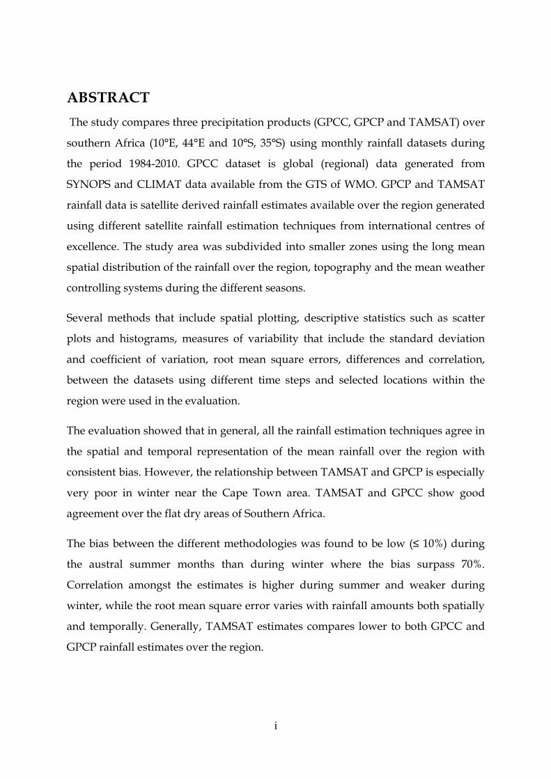
ABSTRACT

The study compares three precipitation products (GPCC, GPCP and TAMSAT) over

southern Africa (10°E, 44°E and 10°S, 35°S) using monthly rainfall datasets during

the period 1984-2010. GPCC dataset is global (regional) data generated from

SYNOPS and CLIMAT data available from the GTS of WMO. GPCP and TAMSAT

rainfall data is satellite derived rainfall estimates available over the region generated

using different satellite rainfall estimation techniques from international centres of

excellence. The study area was subdivided into smaller zones using the long mean

spatial distribution of the rainfall over the region, topography and the mean weather

controlling systems during the different seasons.

Several methods that include spatial plotting, descriptive statistics such as scatter

plots and histograms, measures of variability that include the standard deviation

and coefficient of variation, root mean square errors, differences and correlation,

between the datasets using different time steps and selected locations within the

region were used in the evaluation.

The evaluation showed that in general, all the rainfall estimation techniques agree in

the spatial and temporal representation of the mean rainfall over the region with

consistent bias. However, the relationship between TAMSAT and GPCP is especially

very poor in winter near the Cape Town area. TAMSAT and GPCC show good

agreement over the flat dry areas of Southern Africa.

The bias between the different methodologies was found to be low (≤ 10%) during

the austral summer months than during winter where the bias surpass 70%.

Correlation amongst the estimates is higher during summer and weaker during

winter, while the root mean square error varies with rainfall amounts both spatially

and temporally. Generally, TAMSAT estimates compares lower to both GPCC and

GPCP rainfall estimates over the region.

ii

Acknowledgements

I would like to express my sincere appreciation to all my supervisors, Prof Allan

Richard P., Dr Black Emily and Dr Maidment Ross for their guidance, support and

cooperation throughout my dissertation preparation. Special thank you to Dr.

Maidment Ross who provided technical support in using the data analysis tools (R

Software) and always willing to lend a hand.

Special recognition goes to the UK Met Office and the WMO who provided the

financial support that enabled my study, I say “thank you so much”. I also extend

special thanks to the Government of the Kingdom of Swaziland, Swaziland

Meteorological Services, for being supportive and allowing me time off to further

my studies.

Many thanks go to all the teaching staff of the University of Reading for their

guidance and support throughout the course, especially my course tutor Mr. Ross

Reynolds.

Lastly, would like to extend special thank you to my family and friends for all the

support they extended to me during my studies.

“PRAISE BE TO THE LORD, GOD BLESS US ALL”

iii

LIST OF ACRONYMS

AMESD AFRICA MONITORING OF ENVIRONMENT FOR SUSTAINABLE DEVELOPMENT

CCAFS CLIMATE CHANGE AGRICULTURE FOOD SECURITY

CCD COLD CLOUD DURATION

CLIMAT WMO CODE FOR REPORTING MONTHLY METEOROLOGICAL PAREMETERS FROM LAND AND OCEAN STATIONS

CPC CLIMATE PREDICTION CENTRE

ENSO SOI EL NINO SOUTHERN OSCILLATION INDICES

EO EARTH OBSERVATIONS

EUC EUROPEAN UNION COMMUNITY

FOV FIELD OF VIEW

GCOS GLOBAL CLIMATE OBSERVATIONS SYSTEM

GEWEX GLOBAL ENERGY AND WATER EXPERINMENT

GPCC GLOBAL PRECIPITATION CLIMATOLOGY CENTRE

GPCP GLOBAL CLIMATOLOGY PRECIPITATION PROJECT

GPS GEOGRAPHIC POSITIONING SYSTEM

GTS GLOBAL TELECOMMUNICATIONS SYSTEM

IODZM INDIAN OCEAN DIPOLE / ZONAL MODE

IPCC INTER GOVERNMENTAL PANEL ON CLIMATE CHANGE

ITCZ INTER TROPICAL CONVERGENCE ZONE

JCR JOINT RESEARCH COUNCIL

K KELVIN (TEMPERATURE SCALE)

LDC LEAST DEVELOPING COUNTRIES

MCC MESOSCALE CONVECTIVE COMPLEXES

MFG /MSG METEOSAT FIRST/SECOND GENERATION

MJO MADDEN JULIAN OSCILLATION

NSI NASH SUTCLIFFE INDEX

iv

SADC RSAP & RIP SOUTHERN AFRICA COMMUNITY REGIONAL STRATEGY PAPER AND REGIONAL INDICATOR PLAN

SAH SOUTH ATLANTIC HIGH

SAFFG SOUTHERN AFRICA FLASH FLOOD GUIDANCE

SST SEA SURFACE TEMPERATURE

SYNOP SURFACE SYNOPTIC OBSERVATIONS (WMO CODE)

TAMSAT TROPICAL APPLICATIONS OF METEOROLOGICAL SATELLITES

TIR THERMAL INFRA RED

UK UNITED KINGDOM

UV ULTRA VIOLET

WCRD WORLD CLIMATE RESEARCH PROGRAMME

WMO WORLD METEOROLOGICAL ORGANIZATON

Contents

1 INTRODUCTION ............................................................................................................. 1

1.1 MOTIVATION .......................................................................................................... 4

1.2 OBJECTIVES .............................................................................................................. 8

1.3 AREA OF STUDY ..................................................................................................... 9

2 CLIMATE OVER SOUTHERN AFRICA .................................................................... 11

2.1 OCEANS INFLUENCE .......................................................................................... 14

2.2 El NINO SOUTHERN OSCILLATION INDEX (ENSO-SOI) ........................... 14

3 RAINFALL MEASUREMENTS AND ESTIMATION ............................................ 17

3.1 RAIN GAUGES ....................................................................................................... 17

3.2 SATELLITE OBSERVATIONS .............................................................................. 19

3.3 TYPES OF SENSOR TECHNOLOGY .................................................................. 21

3.4 TYPES OF SATELLITES ......................................................................................... 22

3.5 WEATHER RADAR ............................................................................................... 24

4 RAINFALL ESTIMATION TECHNIQUES ............................................................... 26

4.1 MEASUREMENTS AND ESTIMATION INTERCOMPARISON ................... 26

4.2 TAMSAT RAINFALL ESTIMATION .................................................................. 28

4.3 GLOBAL PRECIPITATION CLIMATOLOGY CENTRE (GPCC) ................... 30

4.4 GLOBAL PRECIPITATION CLIMATOLOGY PROJECT (GPCP) .................. 31

5 DATA AND METHODOLOGY ................................................................................... 33

5.1 DATA ........................................................................................................................ 34

5.2 UNCERTAITY RELATED TO DATA GENERATION ...................................... 36

5.3 METHODOLOGY ................................................................................................... 37

6 RESULTS, DATA ANALYSIS AND DISCUSSIONS ............................................. 41

6.1 RAINFALL AMOUNTS ......................................................................................... 41

6.2 SPATIAL VARIATIONS ........................................................................................ 43

6.3 TEMPORAL VARIABILITY .................................................................................. 48

6.4 MONTHLY AND SEASONAL VARIATIONS .................................................. 50

6.5 VARIATIONS IN SELECTED ZONES ................................................................ 54

7 DISCUSSIONS AND CONCLUSIONS ..................................................................... 59

BIBLIOGRAPHY.................................................................................................................. 64

vi

1

1 INTRODUCTION

The successful application of weather and climate information to decision making

and planning is dependent upon understanding this information which increases its

economic value and its appropriate use. The economic value tends to increase with

the quality, accuracy, timeliness, and location specificity and user-friendliness of the

weather and climate information. Such an assertion is evident in a report “Weather

Information for Development” (WIND, 2011) focussing on improving the livelihoods

of small holder farms through the provision of improved weather and climate

information in East Africa. The farmers stressed their need for better weather

information to plan better farming throughout the year and enable effective use of

resources such as in ploughing, planting, weeding and harvesting of crops, minimize

risks and improve credit worthiness.

In southern Africa, which is composed mainly of least developed countries (LDC’s)

with about 45% of the population living with less than 1(one) $US a day according to

Southern Africa Development Community Regional Strategy Paper and Regional

Indication Plan March 2010 (SADC RSAP & RIP, 2010), over 95 % of the land used

for food production is dependent on rain fed agriculture. The vegetation in this

region consists of mainly annual plants which feed both domestic and wild animals

many tourists from countries where these species do not exists, visit southern Africa

to have a glimpse of them. Such plants closely follow the rainfall seasonality

(Chikoore and Jury, 2010), germinating after the first rains, and unless affected by

disease or die before maturity because of lack of water (rainfall), these plants will

reach senescence after maturing of their fruits (which is also a function of

temperature and light) to mark the end of the rainy season. This makes information

on rainfall information indispensable both in space and time over the region for the

ecosystem and economic growth at large.

The region is particularly very vulnerable to adverse effects of climatic change (Boko

et al., 2007). The vulnerability of the sub-continent is exacerbated by its high level of

dependency on natural and agricultural resources for fresh water including its low

2

adaptive ability to changes because of multiple stresses such as the extreme poverty.

Indeed other stresses such as environment degradation and uncertainties

surrounding land transformation add salt to the injury. In addition, it is understood

and established that future global warming may cause intensification of the

hydrological cycle (Trenberth et al., 2007, Zahn and Allan, 2013) leading to changes

in normal weather including frequencies of extreme events which calls for

intensified planning for adaptation.

In recent decades, southern Africa experienced worst summer drought (1982/83 and

1991/92) associated with extreme El Nino events that caused severe fall in livestock

and crop production which led to severe food shortage prompting the launch of a

series of international humanitarian appeals aimed more fundamentally at averting

the consequences of regional famine and widespread human suffering (Holloway,

2003). Such events are expected to be on the increase with global warming

accelerating climate change (Meehl et al., 2007), and there is general consensus that

agricultural production and food security in many countries and regions is likely to

be severely compromised with projected reductions in yield in some countries

reaching as much as 50% by 2020. This could further lead to falls in net crop

revenues by as much as 90% by 2100, with small-scale farmers being the most

affected.

Apart from agriculture, reports from other sectors show evidence of susceptibility of

communities in the region to climate variability and change such as the report from

the World Meteorological Organisation (WMO) Disaster Risk Reduction Programme

(WMO DRRP) by the Centre for Epidemiology and Disasters for the period 1980–

2007 (http://www.wmo.int/pages/prog/drr/). This report show that during the

aforementioned period, 90% of the reported disasters were natural hazards related

to weather and climate such as floods, drought, water-borne diseases and insect

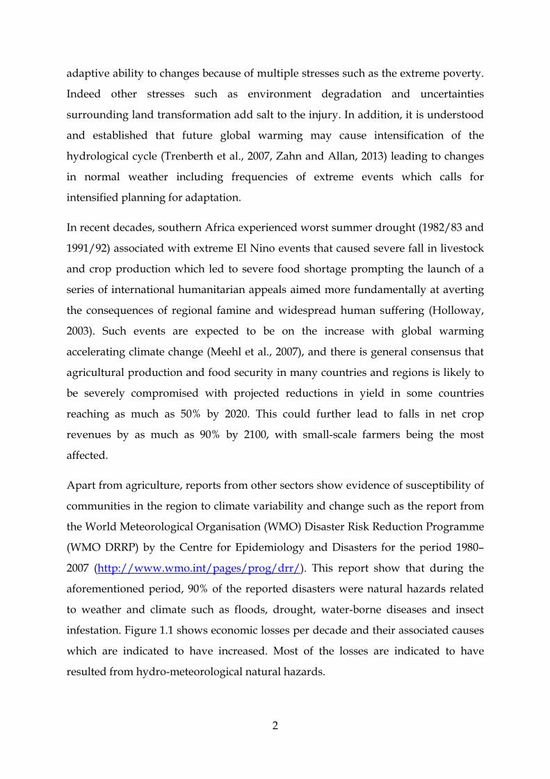
infestation. Figure 1.1 shows economic losses per decade and their associated causes

which are indicated to have increased. Most of the losses are indicated to have

resulted from hydro-meteorological natural hazards.

3

Figure 1.1: Decadal trends in natural hazards impacts over the last 50 years indicating a rise in economic losses associated with hydro-meteorological hazards (Golnaraghi et al., 2009)

In the year 2000, the worst floods occurred in Mozambique displacing and rendering

multitudes of peoples homeless including 929 losses of lives which have been

attributed to consequences of environmental change (Arnell, 2002). Resistance and

resilience in communities and these sectors can be improved through availability of

reliable and accurate climatic information. The availability of such information is

helpful in the development of an early warning systems to mitigate effects of these

disasters and unexpected shocks (Ogallo, 2010). The region information centres

grapples with inconsistent and unreliable weather and climate information which

compromise and hinders the provision of information for regional planning on

climate change adaptation and disaster risk reduction to member states.

This dissertation project assesses TAMSAT satellite-derived rainfall dataset for

Africa and compares it with two global community based rainfall datasets

4

commonly used. It seeks to understand and evaluate the relative strengths and

weaknesses of these rainfall products with the aim of providing quantitative

information that may be necessary and useful for the product improvement and

improve applicability. During the evaluation, links between rainfall estimates and

subsequent climatic features will be investigated in order to identify deficiencies in

the rainfall estimates in capturing the particular events with aim of providing

feedback information for the improvement of the satellite estimation methods. Apart

from providing information for improvements of the estimates, understanding the

relative strengths and weaknesses of these estimates will provide useful information

for the users of the information to derive full economic value from the information

and apply the information appropriately.

The detailed motivation to this dissertation project is provided below together with

the objectives of the study and details of study area. The rest of the sections in this

document will be structured as follows; the second chapter provide information on

the general weather and climate controlling systems over southern Africa. The third

chapter provides literature on the surface rainfall measurement including satellite

observations and different types of satellites in constellation. Chapter 4 provide

details of the methodologies used to generate the different datasets used in the study

including known uncertainties in the different methodologies and their understood

sources. Chapter five provide the data analysis methodologies which are followed

by results and analysis in chapter 6, before concluding and giving suggestions for

the future in section 7.

1.1 MOTIVATION

Rainfall is the primary source of fresh water for consumption and to support

vegetative growth and agriculture over southern Africa like in many in many parts of

the world. This makes monitoring its distribution, amount and intensity essential for

planning its full utilization, taking into consideration that the region is mainly semi

arid. Apart from planning its utilization as input for agricultural produce, information

on rainfall is useful for simulating the land-surface hydrologic processes, predicting

5

drought and flood, monitoring the water resources state and supporting appropriate

studies for the understanding of climate variability and change (Washington et al.,

2006). Despite the importance of rainfall information and its usefulness to the

community livelihoods, the southern Africa region is far from attaining an adequate

level of monitoring of rainfall to meet the user needs both with the provision of

quality information for socio economic growth and safety of life and property. This is

partly due to the prevailing economic situation faced by most countries and other

more demanding social hardships such as provision of primary health care services,

primary education, and economic recessions (SADC RSAP & RIP 2010).

The current meteorological observing systems in the region fall short of meeting

desired climate information needs as a result of the inadequate station network,

instruments and system failure, lack of proper maintenance and calibration which is

compounded by shortage of skilled staff and inefficient communication

infrastructure for collecting and exchange of data. The African Climate Report

(Washington et al., 2006) found the climate observing system for Africa in a rather

worse state than in any other continent. Similar conclusions were made by

(Sawunyama and Hughes, 2008) who observed a sharp decline of the active rain-

gauge network over many developing countries including Africa and the available

rainfall data unevenly distributed and most gauging stations located in towns and

along roadsides. There is very little hope that the surface observations network will

improve in the foreseeable future, considering the many economic situations in these

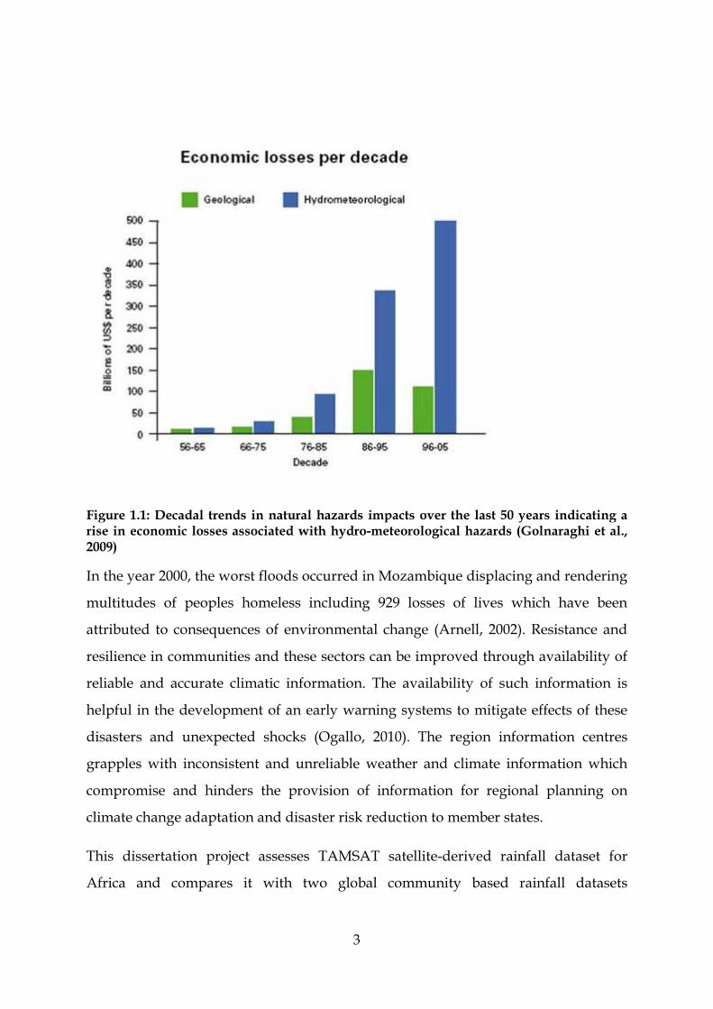
countries. Evidence of the unreliable and unsatisfactory gauge observations in the

region can be seen from the GPCC monitoring reports. Figure 1.2 provides an

example of available gauge data from southern Africa at the GPCC monitoring

centre for day selected randomly. A number of trials randomly selecting days were

performed, with no improvement in the sampling. A vast area of the subcontinent

shows unavailability of gauge reports which affect planning and providing

advisories on rainfall and related operations.

6

Figure 1.2: Map showing of number rain gauge network reports from southern Africa available in the GPCC monitoring

Through the advance in remote sensing technology and active participation of

scientists from around the globe who seek to understand of the underlying key

climate processes, (e.g. EUMETSAT, GEWEX, TAMSAT, and EU Joint Research

Council JCR), and use of their scientific knowledge resulted in development of

models that simulate the earth’s climate system and derivation of rainfall from

clouds using the remote sensing techniques. Given the sparse surface observation

network, remote sensing techniques offer the only method of observing rainfall over

all of Africa. This technology offers continuous observations in near-real time such

as MSG observations that are currently updated every 15 minutes at a fine enough

spatial resolution e.g. 0.0375° to be of use in a variety of applications. The satellite

7

rainfall estimates have become increasingly available and accessible in near real

time, their accuracy continuously improving as shown in a number of studies

evaluating satellite rainfall estimates (e.g. Adler and Negri, 1988; Xie et al., 2003;

Thorne et al., 2001; Bell and Kundu, 2003; Yilmaz, 2005; Roca et al., 2009; Maidment

et al., 2012). The satellite rainfall estimates have become a viable data source for a

wide range of applications, including studies on the physical climate system

(Stephens and Kummerow, 2007), creating rainfall maps that are critical for the

investigation of scientific issues such as hydrological regimes (Xie et al., 2003),

(Yilmaz et al., 2005), delineating marginal lands and mapping flood prone areas,

early warning and food security (Yilmaz et al., 2005), (Pierre et al., 2011).

The Tropical Applications of Meteorological using Satellite and ground based

observations (TAMSAT) Group from the University of Reading, UK has been

producing operational rainfall derived from METEOSAT thermal infra (TIR) images

for northern Africa since 1988 and for southern Africa since 1993 (Thorne et al.,

2001). These dekadal rainfall estimates for Africa have shown to perform well over

most areas over Sub – Sahara Africa (Dinku et al., 2007, Jobard et al., 2011, Maidment

et al., 2012) which gives confidence in the application of these estimates. The

TAMSAT group recently developed two new methods based on TAMSAT decadal

estimates to generate daily rainfall estimates for Africa spaning nearly 30 years

(CCAFS, 2012 pdf). Creation of datasets from satellites enhances usefulness of

precipitation data and provides an alternative method for providing timely, reliable

and homogeneous records. Such data are of particular importance to overcoming

other deficiencies such as the declining conventional operational rain gauges

network over the continent.

The TAMSAT rainfall estimates have been made available to Southern Africa

through the Africa Monitoring of Environment for Sustainable Development

(AMESD) initiative that makes use of earth observations (EO) technologies and data

set up operational environment and climate monitoring applications with funding

from the European Union Community (EUC). This initiative aims at providing all

African nations with the resources necessary to manage the environment effectively

8

ensuring long term sustainability through full access to environmental data and

products required to improve national and regional policy and decision making

process. Proper application of the technology comes with understanding its

strengths and weaknesses to be able to apply it effectively such as climate variability

and change advisories. Currently remote sensing technology is the only available

efficient means (Grimes et al., 1999) of ensuring adequacy of climate observing

systems and is the only affordable way of monitoring environmental conditions over

a large area in real-time.

Notwithstanding the advancement in the remote sensing technology and the fact

that a large amount of work has been put into reducing discrepancies between

satellite rainfall estimates and ground observations during the calibration processes

(Dinku et al., 2007), the rainfall estimates still need to be validated against ground

observations to increase the understanding of their quality and quantify the level of

uncertainty for appropriate use and confidence in their different application.

Understanding the discrepancies between the satellite rainfall estimates and

observations is achieved through quantitatively evaluating these rainfall estimates

and assessing their relative strengths and weaknesses (Thiemig et al., 2012). By

comparing these sets of estimates and understanding the spread amongst them

indirectly measures the effect of the different physical assumptions in the retrievals,

impacts of different sampling strategies or limitations and effect of the various

merger schemes. Assessing these estimates improves the confidence in their

application and usefulness including increasing ability to assist other users with

reliable information required for disaster mitigation through proper planning,

poverty alleviation improved food security in the region.

1.2 OBJECTIVES

This study aims at contributing to the scientific base necessary for understanding

and assessing the level of skill of the different satellite rainfall estimates by

comparison with gridded rain gauge data over Africa with specific focus over

Southern Africa region. The specific objectives are;

9

• Ascertain level of skill of rainfall estimates over Southern Africa for provision of

high resolution gridded data sets for numerical model inputs, climate

monitoring, detection and attribution

• Understand rainfall variability; detect trends, persistence and any cyclic

variations in the rainfall with specific applications to agriculture and fresh water

monitoring.

• Extended capabilities in monitoring extreme rainfall events and understanding

how the rainfall has changed over time.

1.3 AREA OF STUDY

Figure 1.3 shows the area of focus for the study which is continental southern Africa

bounded by 10°E, 44°E and 10°S, 35°S. Southern Africa climate varies spatially from

arid in the west through semi arid and temperate areas in central zones with sub

humid regions bordering the north and north eastern parts. This region is home to

16.7% of Africa continent population, and generally, it is understood that its climate

is highly variable and complex e.g. ( Thorne et al., 2001, de Coning and Poolman,

2011, Jury et al., 2007, Blamey and Reason, 2012). The region consists of highly

varying topography ranging from mean sea level to about 3000 metres over the

mountains and is bounded by the relatively warm Indian Ocean to the East and mild

Atlantic Ocean to its West. Drought events over the region have been found to be on

the increase in recent years (Rouault and Richard, 2005), and the region is widely

recognised as one of the most vulnerable regions to climate variability and climate

change as discussed in section 1 on a range of time scales because of low levels of

adaptive capacity (particularly among rural communities), combined with a high

dependence on rain-fed agriculture (IPCC, 2007).

10

Figure 1.3: Map of Southern Africa and its surrounding oceans with countries found in the region

11

2 CLIMATE OVER SOUTHERN AFRICA

A larger part of Southern Africa and its adjacent Atlantic and Indian Oceans are

located in the region of large – scale subsidence occurring between the Hadley and

Ferrel cells of the Southern Hemisphere general circulation which accounts for its

climate being generally arid to semi arid (Kidson and Newell, 1977). A combination

of complex factors as shown in figure 2.1 that include the geographic location,

variations in regional topography and sea surface temperatures, the tapering of the

subcontinent result in subtropical southern Africa experiences considerable spatial

and temporal variability in rainfall. At shorter temporal or synoptic time scales, the

observed variability of rainfall can be linked to both tropical waves’ dynamics and

mid latitude air intrusion (Chikoore and Jury, 2010).

Figure 2.1: Map of the main weather and climate features over southern Africa during the austral summer. The broad dashed line lying diagonally across the sub continent represents mean position of convergence associated with convective bands during the period (Blamey and Reason, 2012).

12

Over this region, most of the rainfall occurs during the austral summer as shown in

figure 2.2 in the form of convective thunderstorms associated with the seasonal

mach (relative migration) of the Inter Tropical Convergence Zone (ITCZ) (Preston-

Whyte and Tyson, 1988); (Lindesay and Bridgman, 1998).

Figure 2.2: Mean annual rainfall distribution for the area bounded by 10°E, 44°E and 10°S, 35°S southern Africa) showing maximum rainfall between DJF when ITCZ has maximum extent to the southern hemisphere. Figure (a) graph of mean monthly GPCC and TAMSAT data at 0.5 degree grid scale; (b) mean monthly GPCP and TAMSAT data at 2.5 degree grid scale.

The ITCZ is a near equatorial trough in which tropical easterly flow from the north

and south of the equator converge. During the southern hemisphere summer, the

ITCZ lies south of the equator and has maximum southward displacement over

south east Africa where it is displaced as much as 20°S (Lindesay and Vogel, 1990).

During this period, the tropical temperate troughs have their maximum effect on the

region with associated northwest – southeast cloud bands developing and

dominating the summer rainfall. These meso-scale convective complexes (MCC)

have been studied by (Blamey and Reason, 2012) who found that they tend to

develop along the temperate tropical trough influencing rainfall over central

Mozambique extending south to Swaziland. High precipitation totals have been

associated with these systems which also occur over the neighbouring South West

13

Indian Ocean, particularly off the north east coast of South Africa. These contribute

up to about 20% of the total summer rainfall (November – March) in parts of the

eastern region of southern Africa.

Within the seasonal cycle there is alternating sequence of wet and dry spells which

at times extend for more than a month with critical implications to rain fed

agriculture (Tennant and Hewitson, 2002). The dry spells are associated with the

development of an intense mid-troposphere anticyclone often referred to by the local

meteorological community as the Botswana upper high pressure associated with the

Kalahari desert which causes large scale subsidence over adjacent the sub continent.

There also exist intra-seasonal cycles with fluctuations that have eastward moving

areas of zonal winds, moisture convergence and surface pressure in the tropical zone

that brings rain every 30 – 60 days associated with the Madden – Julian Oscillation

(MJO) which studies have found to be prevalent mainly during wet years over

southern Africa (Chikoore and Jury, 2010).

Over the western parts of the subcontinent, the ITCZ southward shift is not as

pronounced as over the eastern parts of the region due to the relatively weak

changes in the intensity of the Atlantic Ocean central pressure and strength (Reason

et al., 2006). A pronounced seasonal difference in rainfall patterns exists in southern

Africa that is related to the influence of the ITCZ and the annual cycle of the semi

permanent anticyclones. The extreme south western parts of southern Africa

receives much of rainfall during austral winter due to influence of mid latitude

migratory weather patterns associated with cold fronts and ridging of high pressure

behind causing influx of low level moisture inland.

The steep topography of the eastern escarpment, sub-tropical easterly flow, and

contrasting warm Indian and cool Atlantic oceans, ensure sharp gradients in rainfall

with semi arid conditions along the western boundary. The difference in heat

capacities between land and water bodies maintains gradients of temperatures

between the land and the ocean generating localised circulation. The rainfall is

14

characterized by strong seasonal cycle with a well defined wet season (October –

April) over most of the subcontinent (Reason et al., 2006).

2.1 OCEANS INFLUENCE

Recent studies have focussed on enhanced understanding of the links between the

local oceans and their contributions in the evolution of the weather and climate over

the region e.g. (Saji et al., 1999, Annamalai and Murtugudde, 2004, Cook et al., 2004,

Song et al., 2008, Manatsa et al., 2012). There has been found the existence of an east

– west mode of variability of the Indian Ocean Dipole / Zonal Mode (IODZM) that

has influence on rainfall variability over parts of Southern Africa. The IODZM is

described as the extreme sea surface cooling events that occur during the boreal

autumn in the eastern tropical Indian Ocean that arises from coupled atmospheric

feedbacks that result in an east – west sea surface temperature gradient along the

tropical Indian Ocean (Saji et al., 1999). The positive phase of the IODZM is

associated with the westward shift of convection over the eastern Indian Ocean

resulting more rainfall over eastern southern Africa, thus the alternating warm (cool)

sea surface temperatures to the east and cool (warm) sea surface temperature to the

west result in wet(dry) spells. Over the western southern Africa on average, the

Atlantic Ocean anticyclone shifts only about 6° latitude between seasons with

significant semi-annual oscillation in position (Reason et al., 2006). The seasonal

fluctuations in the anticyclone drive changes in the surface winds and hence SST’s,

particularly in the upwelling zones along the west coast of southern Africa such as

along the Namibian coast during the winter months. These oceans act as sources of

low level moisture and have high influence on the climate of Southern Africa both at

synoptic and seasonal time scales.

2.2 El NINO SOUTHERN OSCILLATION INDEX (ENSO-SOI)

The El Nino Southern Oscillation Index (ENSO-SOI) is widely understood and

accepted to be highly associated with the inter-annual rainfall variability over

Southern Africa including patterns of tropical sea surface temperature (SST) and

zonal overturning circulations e.g. (Richard et al., 2000, Ropelewski and Halpert,

15

1987, Ropelewski and Halpert, 1989, Reason and Rouault, 2002, Jury et al., 2002).

ENSO, primarily a tropical Pacific phenomenon, is thought to influence southern

Africa weather patterns through modulation of the local Walker circulation and SSTs

in the neighbouring Indian and Atlantic Oceans; (Janowiak, 1988), (Fauchereau et al.,

2009). Figure 2.3 show the general global conditions of moisture and temperature

associated with warm El Nino episodes. During ENSO modes, parts of Southern

Africa remain under warm and dry conditions such as was the case described in

above that resulted in the worst drought that affected the region in recent times. The

El Nino causes the south Indian Ocean convergence zone to be displaced and shifted

north eastwards and positioned over the Indian Ocean, resulting in reduction of

moisture convergence, uplift and instability that result in dry conditions prevailing

over southern Africa. However, the relationship between rainfall over southern

Africa in non linear (Mason and Goddard, 2001, Reason and Jagadheesha, 2005) as

was shown by the 1997 El Nino phase which failed to produce the known results

prompting further investigations into the El Nino characters and its relationship to

the region precipitation (Mason and Goddard, 2001, Reason and Jagadheesha, 2005).

Figure 2.3: Warm and dry conditions in December - February prevail over Southern Africa during a warm El Nino Episode. During warm ENSO episodes the normal patterns of tropical precipitation and atmospheric circulation become disrupted. Source: NCDC NOAA

16

The reversal of the El Nino (La Nina) phase is associated with reversed conditions

over the region, such that during these years the south Indian Ocean convergence

zone tends to be located over the continent resulting in generally wet conditions

over most parts of the sub-continent as shown in figure 2.4 which depict mean global

conditions associated with La Nina.

Figure 2.4: Map showing parts of Southern Africa covered by wet and cool conditions in December - February during La Nina episodes. During La Nina episodes the normal patterns of tropical precipitation and atmospheric circulations become disrupted. Source, http://www.ncdc.noaa.gov/

17

3 RAINFALL MEASUREMENTS AND ESTIMATION

Since rainfall is one of the most important parameters affecting human life its

measurement has been pursued for a long time. As discussed in section 2, rainfall is

variable both in space and in time making accurate measurements and

representation difficult. Rainfall measured at a point is very different from over an

area, hence spatial interpolation for inter comparison studies is required (e.g. Thorne

et al. 2001, Ali et al., 2005, Pierre et al., 2011). Because of its importance to human life,

man has developed different techniques for rainfall measurements ranging from

planting gauging system on the ground to intercept the falling rain using a simple

bucket with collecting funnel, storage and a measuring cylinder to sophisticated

ground and space–borne using complex science and mathematical equations to

provide information on rainfall both in space and in time (Adler et al., 2003). These

different systems have their merits and limitations which are discussed in detail

below.

3.1 RAIN GAUGES

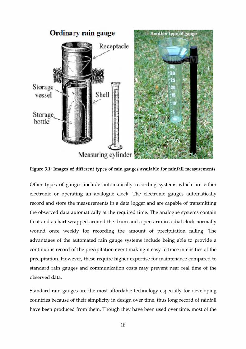
Different rain gauge designs as shown in figure 3.1 below have evolved and existed

over time in different regions and countries, and at times different designs exist and

are used within country. These different designs however, can make comparisons of

rainfall data very difficult especially where the information about the measurements

is not provided to quantify the uncertainties related to these measurements (Arnell,

2002). The most common and simplest is a non recording cylindrical container of

defined height with an orifice of a defined size that collects rainfall (Strangeways,

2007). The collected rainfall is emptied into an accompanying measuring cylinder for

measurements usually at fixed time intervals.

18

Figure 3.1: Images of different types of rain gauges available for rainfall measurements.

Other types of gauges include automatically recording systems which are either

electronic or operating an analogue clock. The electronic gauges automatically

record and store the measurements in a data logger and are capable of transmitting

the observed data automatically at the required time. The analogue systems contain

float and a chart wrapped around the drum and a pen arm in a dial clock normally

wound once weekly for recording the amount of precipitation falling. The

advantages of the automated rain gauge systems include being able to provide a

continuous record of the precipitation event making it easy to trace intensities of the

precipitation. However, these require higher expertise for maintenance compared to

standard rain gauges and communication costs may prevent near real time of the

observed data.

Standard rain gauges are the most affordable technology especially for developing

countries because of their simplicity in design over time, thus long record of rainfall

have been produced from them. Though they have been used over time, most of the

19

rainfall record from standard rain gauges is susceptible to a number of errors (Habib

et al., 2001) resulting from a number of varied reasons such as those related to

installation and human error mainly due to incompetent observers taking the

measurements. Even in gauges that are properly maintained, errors arise from both

random and systematic components depending on the type of apparatus, the

surrounding environment and the type of rainfall being measured. Aerodynamic

effects are often the most common and can lead to underestimates of rainfall

depending on the rate of the rainfall, wind speed, gauge type and exposure of the

rain gauge. Apart from the errors associated with rain gauge measurements, rain

gauges have a major disadvantage in aerial rainfall representation. Rain gauges

measure precipitation falling within the diameter of the gauge (Huffman et al., 1995).

Inferences to what may have fallen squares of kilometres around the gauge can only

be made to the extent to what the gauge encounters is representative of what

happened in the surrounding area.

However, gauge data provides the only means of verifying (ground truth) satellite

derived rainfall data. But the distribution of the gauges (Ali et al., 2005) and how

well these gauges agree amongst themselves (Rudolf et al. 1994) has an effect on the

estimation errors of the satellite rainfall estimates. Greater variations in mean

precipitation values amongst satellite estimates over the ocean were observed

(Adler et al., (2011) compared to overland estimates where there is good gauge

measurements and information.

3.2 SATELLITE OBSERVATIONS

Satellite are the only practicable means of observing rainfall continuously on a larger

scale, but the remote sensing methods used in estimating rainfall from space borne

instruments are inexact as explained below. Satellite observations of the earth’s

atmosphere are in the form of spectral radiance or irradiance arising as natural

processes of emission and scattering of electromagnetic radiation by an object in the

atmosphere or over a geographical area on the surface. The satellite measuring

technique is based on the principle of black body laws of physics which in its

20

simplicity relates emission and temperature. All objects emit electromagnetic

radiation and the type of radiation they emit depends on their temperature as shown

in figure 3.2a below. The hotter the object the more intense the radiation emitted and

the greater the proportion of radiation emitted at shorter wavelengths. The surface

of the Sun is at a temperature of about 6,000 °C and it emits predominantly in the

visible region of the spectrum. The Earth has an average temperature of about 15 °C

and emits mainly in the infra-red and microwave regions.

Given the inherent nature of the interactions between different bodies such as clouds

and precipitation and the electromagnetic radiation, vary according to spectral

region of interest (figure 3.2b), then it is expected that the information content in

such observations also varies according to where in the spectral region the

observations are performed.

Figure 3.2: A diagram of the electromagnetic spectrum showing various properties across a range of wavelengths. (a) Show energy sources, (b) shows atmospheric windows (transmittance) and (c) indicates common remote sensing systems and wavelengths used. The main wavebands used in cloud measurements are highlighted in colour,

21

One class of approach for information retrieval relies on measurements of

transmission where the attenuation of the defined source of radiation is used to

determine some properties of clouds, while the other method utilizes the scattered

radiation by clouds and precipitation (Lillesand et al., 2004).

3.3 TYPES OF SENSOR TECHNOLOGY

Different sensor technologies carried on board the different remote sensing

platforms have evolved such as explained by Adler and Negri, (1988), Stephens and

Kummerow, (2007), Yong et al., (2010), and used to acquire the information at these

different wavelengths. The most common ones for meteorological applications are

discussed below and include;

i) VISIBLE (VIS) SENSOR (0.4 – 0.7µm)

Visible sensors record the reflected light from the sun by the cloud tops, land and sea

surface. Rainfall estimation depends on cloud optical depth, cloud phase, cloud

particle sizes and distribution. This sensor type picks information from clouds using

their different reflecting properties to the land and sea. However, visible sensor only

provides information during daytime and the observations from this type of sensor

only relate to characteristics of cloud tops, rather than the precipitation reaching the

ground.

ii) INFRA–RED (IR) SENSORS (9 - 12µm)

This type of sensor records the emitted radiation by clouds, land or sea surface. As

explained in section 3.2 above, infra red sensors utilize the part of the spectrum

beyond the visible wavelength of light and the atmosphere transmission

(atmospheric windows). The most used channel for rainfall estimation of the

electromagnetic spectrum is IR 10.8µ. Similarly, IR sensor technology only relate to

characteristics of cloud tops rather than the rainfall reaching the ground.

iii) PASSIVE MICROWAVE SENSORS (PMW)

22

The atmosphere optical window is not the only region of the electromagnetic

spectrum that is used for meteorological and hydrological applications. Microwave

sensors on board polar orbiting satellites commonly utilize the microwave (mw)

wavelengths (~ 1cm) to exploit the atmosphere transparent window located at these

wavelengths as shown in figure 3.2c of the spectrum and the fact that each height in

the atmosphere is sensitive to a slightly different wavelength of radiation.

Observations at microwave frequencies relate to the amount of water within the

vertical column of the atmosphere being observed. At these wavelengths, clouds

appear mostly transparent, thus the sensor can obtain information from underneath

the cloud layer. These sensors are referred to as passive sensors since they measure

the natural radiation emitted or scattered (re-directing) from the atmosphere beneath

the sensor.

The remote sensing technology applied to rainfall estimation been in use for some

time and ranging from relatively simple empirically derived and calibrated

techniques such as the TAMSAT algorithm (Grimes et al., 1999), through to those

that use complex atmospheric physics and radiative transfer equations. These have

been applied to support of a variety of applications such as climate studies, input

into agriculture, hydrological and weather forecasting. They have been useful in

compensating for unreliable sparse and late reporting gauge stations especially in

developing countries for early warning systems and decision making process e.g.

(Arkin and Meisner, 1987, Adler and Negri, 1988, Kummerow et al., 2001).

3.4 TYPES OF SATELLITES

Different types of satellites are in existence and operated by different space agencies

and different applications. For meteorological applications relevant to the study, two

types of satellites will be discussed.

i) GEOSTATIONARY SATELLITES

A geostationary satellite has a geosynchronous orbit which implies that the satellite

is always in the same position with respect to the rotating earth. The current

23

generation of geostationary satellites orbit the earth at approximately 36,000 km

along the equator (0°) at same period (24 hrs) with the rotating earth which makes

the satellite appear stationary above the earth’s surface. Figure 3.3(a) below

illustrates a geostationary satellite in orbit relative to the rotating earth. The current

operational geostationary satellites providing data for Africa and Europe is the

METEOSAT Second Generation (MSG) which has evolved from first generation

(MFG) and have in total provided satellite observations and subsequent

meteorological products and information for over 30 years. Presently, the

METEOSAT satellites make use of 12 spectral channels and have a spatial resolution

of approximately 3 km at sub satellite point and produces full disk view of Africa

and Europe every 15 minutes making it ideal for monitoring convective

developments especially over Africa where the satellite has a good field of view

(www.eumetsat.int). Geostationary satellites provide better information in the

longer term due to its high temporal resolution.

Figure 3.3: A model of a geostationary satellite in orbit. (b) Field of view of METEOSAT geostationary satellite on 2nd July 2013, 0600Z. Images source: www.eumetsat.int

Full utilization of satellite-based precipitation datasets is hindered by the uncertainty

and reliability associated with the precipitation estimates. One disadvantage of

IR/VIS rainfall estimation technique is that precipitation is inferred from clouds

(Adler and Negri, 1988) which introduces further errors in the measurements and it

is believed that the accuracy of such techniques cannot be readily transferable from

one location to another location.

ii) POLAR ORBITING SATELLITES

24

Polar orbiting satellites are the family of satellites that orbit the earth at lower

altitudes compared to the geostationary satellites at approximately 850km. They pass

over the North Pole and South Pole on each revolution with each revolution taking

about 90-100 minutes. This means that these satellites pass over every point on the

earth’s surface twice each day. Because of their low orbit, polar orbiting satellites

provide much higher spatial resolution information than geostationary satellites.

However, these cannot offer good information for short lived weather and climate

events since they only sample a point on the earth’s surface twice daily during their

overpass carrying on board the passive microwave sensors.

Microwave rainfall retrieval are also affected by so-called beam-filling effect due to

unresolved rainfall heterogeneity within sensor FOV, as well as having a non-linear

relationship between brightness temperatures and high rainfall rate which can result

in bias in estimated rainfall intensity (Curran, 1982) which may contributes to the

error in accumulated rainfall estimates. Furthermore, the emissivity of the land

surface at the microwave spectrum is higher and more variable in space and time

than over the ocean, causing additional complexity of rainfall retrieval over semiarid

regions of Africa. Bellerby and Sun, (2005) suggests that in general, passive

microwave algorithms generally produce overestimates of rainfall. More information

on polar orbiting satellites is available on, http://www.ospo.noaa.gov/

3.5 WEATHER RADAR

Other available technology for rainfall estimation especially in developed countries

is the weather radar. Weather radar is also available in some aircrafts to provide

information on hazardous weather during the aircraft in flight. The weather radar

primary operating principle entails emitting of a beam or pulse of microwave or

radio waves from the radar transmitter into the atmosphere. When the beam collides

with an object on its path such as cloud droplets, solid or liquid rain drops such as

hail stones, some of the energy bounces back to the radar receiver and redetected

and processed in the processing unit and graphically displayed for interpretation.

25

Weather radar, provide a comprehensive picture of the rainfall pattern over an area

and have high temporal resolution. One major non technical disadvantage with

weather radar systems relates to their technical requirements related to installation,

operations and maintenance costs which eliminate developing countries affording

these systems. Over southern Africa, an operational radar network is found in South

Africa which is useful in the South African Flash Flood Guidance (SAFFG) system

(de Coning and Poolman, 2011) and supported by a fairly dense rain gauge network

of about 1500 daily gauges. However, less rain gauge information is exchanged and

made available to the GTS of WMO.

Apart from the non technical disadvantage, radars do not measure precipitation

directly as discussed above. The conversion of the signal backscatter into rain rates is

not exact and the surface affects radar accuracy, such as radar may fail to capture

low level precipitation due to upward refraction of the radar beam (Morin et al.,

2005) through the atmosphere leading to anomalous signals on the radar

measurements.

26

4 RAINFALL ESTIMATION TECHNIQUES

This section discusses the different rainfall estimation techniques available for

producing aerial rainfall relevant to the study and which the data used in this study

was generated.

4.1 MEASUREMENTS AND ESTIMATION INTERCOMPARISON

Though satellite derived rainfall estimates have been available for use in Southern

Africa, e.g. in Zambia, the Meteorological Service distribute 10-day rainfall estimates

and related products for agriculture purposes (Thorne et al., 2001), minimal studies

on these satellite rainfall estimates have been undertaken in southern Africa that

provide information on their uncertainties, relative weaknesses and strengths unlike

in other parts of the African continent such as northern Africa. Over northern Africa

a number satellite rainfall estimates inter comparison studies have been undertaken

e.g. (Herman et al., 1997, GRIMES and DIOP, 2003, Ali et al., 2005, Dinku et al., 2007,

Roca et al., 2009, Roca et al., 2010, Jobard et al., 2011, Owolawi, 2011, Chadwick and

Grimes, 2012, Maidment et al., 2012, Thiemig et al., 2012, Gosset et al., 2013).

Most of the studies are in general agreement that the influence of climate, location,

rainfall types, season and topography and number of gauges within a grid box are

important factors in the performance of satellite algorithm including the spectral

range (IR or PMW) used in the measurements. A number of satellite rainfall

estimates show the effect of the number of rain gauge measurements within each

grid box in the bias error estimates including how the errors improve with increased

density of gauge observations e.g. (Grimes et al., 1999, Thorne et al., 2001, Ali et al.,

2005, Dinku et al., 2007, Maidment et al. 2012, Chadwick and Grimes, 2012). Adler et

al., (2011) estimating climatological bias errors for GPCP argued that higher errors

were found over the ocean than over land, and attributed lower bias error over the

land to availability of gauge information over the land.

In an East Africa validation study, Dinku et al. (2007) found that satellite rainfall

estimates did not compare well with in-situ rain gauge data in a study over regions

of Ethiopia, attributing poor performance mainly to topography. Specifically, they

27

noted that topography plays a significant role in satellite rainfall estimation due to

an algorithm’s inability to detect mountain enhanced rainfall. Similar observations

were found by Romilly and Gebremichael, (2011) over northwest Ethiopia consisting

of mainly highland topography and humid climate strongly influenced by the ITCZ.

Similarly, in the Climate Change, Agriculture and Food Security Technical Report,

(CCAFS, 2012 pdf) suggests that the TAMSAT algorithm is more suited to the Sahel

than East Africa as the occurrence of cold cloud at pixel scale over the Sahel is

closely related to rainfall occurrence than it is over Central and East Africa where the

cold cloud pixel is not always associated with rainfall.

In a study by Thorne et al (2001) over southern Africa which compared TAMSAT

data, Climate Prediction Centre (CPC) and gauge data concluded that TAMSAT

estimation technique of using varying calibration zones performs best over flat and

arid regions and grossly under estimate rainfall over mountainous regions and areas

with very few rain gauges available in real time. Other findings from inter-

comparison studies show that in general, rainfall estimating techniques that include

gauge data compare better e.g. (Dinku et al., 2007 and Jobard et al. 2011), or have

less bias compared to the satellite only rainfall estimates.

However, these it should be noted that these limitations do not particularly imply

that the satellite rainfall estimates cannot represent accurately ground rainfall, but

provide an indication on the weaknesses and sources of uncertainty associated with

the satellite rainfall estimation techniques. Although conclusions have been made

about performance of different estimates and locations, more studies evaluating the

performance of the different algorithms are necessary to enable the continuous

improvements of the satellite rainfall estimates taking into consideration that they

offer measurements even over remote areas particularly over southern Africa where

fewer studies have been carried out.

Most of the studies carried out have considered daily and 10-day rainfall estimates

for the inter-comparison but few have used monthly data and evaluated bias

climatology in the rainfall estimates. It cannot be over emphasised that the most

28

informative comparisons of satellite and rain gauge averages is one where enough

averaging has been done to reduce the variability in the differences due to random

sampling and retrieval error to a level where the residual bias is detectable at a

certain desired level, hence this study is designed to consider monthly and annual

scale of the bias. Bell and Kundu, (2003) in their study comparing satellite rainfall

estimates and gauge data stated that mean differences between gauge and satellite

data can be expected since each of the measurement technique include rain

observations which the other does not include.

4.2 TAMSAT RAINFALL ESTIMATION

The TAMSAT methodology has been described in detail elsewhere e.g. (Milford et

al., 1994, Thorne et al., 2001, GRIMES and DIOP, 2003) but here will give summary

as background information for the study. This method of rainfall estimation utilizes

the 10.8µm infra-red channel from the METEOSAT geostationary satellite and has

data spanning more than 30 years. From this channel, the brightness temperature

can be calculated. This methodology attempts to define a linear relationship between

the numbers of hours for which a satellite pixel temperature is colder than a

specified threshold temperature.

The TAMSAT rainfall estimation technique can be traced back to the work of (Arkin

and Meisner, 1987) who used the idea of Cold Cloud Duration (CCD) to show that

rainfall in the tropical Atlantic could be related to the fractional coverage of cloud

with satellite-measured temperatures below 235K (-38 °C). The TAMSAT algorithm

was initially developed for rainfall estimation over North Africa for agricultural

purposes and predicting famine and floods.

The TAMSAT technique does not merge satellite data with current gauge

observations, but uses historical data that is perceived to be invariant over long time

periods to generate climatological calibrations. The TAMSAT methodology (Grimes

et al., 1999) in its simplicity uses only geostationary IR data on board METEOSAT

satellites and exclusively covers Africa (Thorne et al. 2001). The calibrations are

carried out separately for each calendar month within empirically determined

29

climatic zones. The methodology is perceived to the one of the simplest methods

employed for remotely sensed rainfall which has better performance in rainfall

estimation compared to more complicated methods such as those defined by Adler

and Negri, (1988), Dinku et al., (2007), Chadwick and Grimes, (2012). The detailed

basic assumptions inherent in the TAMSAT rainfall estimation method include as

discussed by Grimes et al., (1999);

• Rainfall predominantly comes from convective clouds.

• Clouds only rain when their tops have reached a certain minimum height

(threshold height)

• Cloud top height can be identified by its temperature on the thermal infra red

(TIR) image referred to as Tt

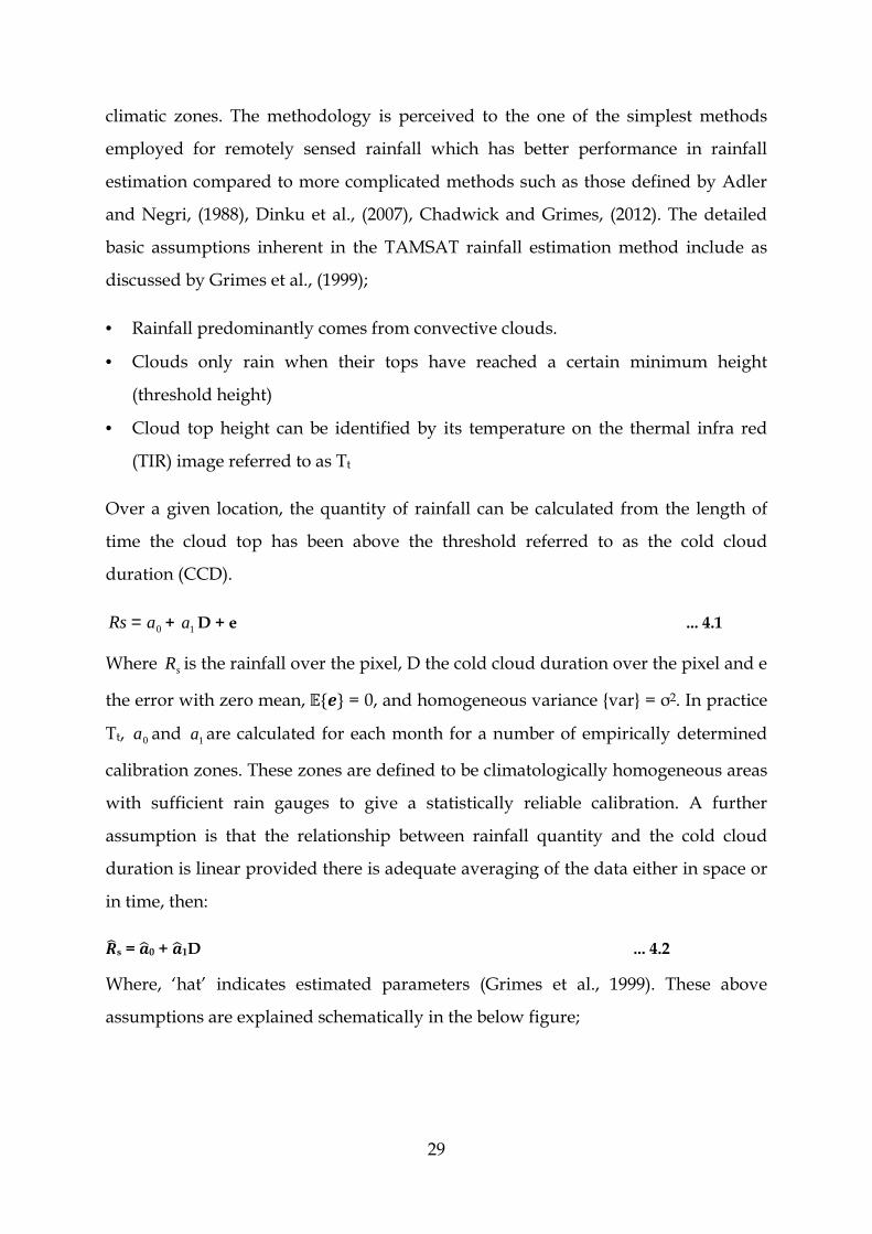
Over a given location, the quantity of rainfall can be calculated from the length of

time the cloud top has been above the threshold referred to as the cold cloud

duration (CCD).

=Rs 0a + 1a D + e ... 4.1

Where sR is the rainfall over the pixel, D the cold cloud duration over the pixel and e

the error with zero mean,�{�} = 0, and homogeneous variance {var} = σ2. In practice

Tt, 0a and 1a are calculated for each month for a number of empirically determined

calibration zones. These zones are defined to be climatologically homogeneous areas

with sufficient rain gauges to give a statistically reliable calibration. A further

assumption is that the relationship between rainfall quantity and the cold cloud

duration is linear provided there is adequate averaging of the data either in space or

in time, then:

��s = �0 + �1D ... 4.2

Where, ‘hat’ indicates estimated parameters (Grimes et al., 1999). These above

assumptions are explained schematically in the below figure;

30

Figure 4.1: Schematic diagram of clouds with tops colder than threshold temperature Tt (dashed line) are assumed to be raining, while clouds with tops warmer than Tt are assumed not to be raining (Grimes et al., 1999).

From the discussions above, some limitations of the TAMSAT algorithm are evident

as is shown by the schematic figure 4.1 above. These errors combined are associated

with identification of cloudy scenes and identification of precipitation from cloudy

scenes and non precipitating cloudy scenes. The problem of discriminating a cloud

clear and cloud precipitating is represented in the above scheme, where small clouds

generating precipitation without reaching the threshold temperature are missed or

regarded as non precipitating clouds. Similarly high level non-precipitating cloud,

when present, may sometimes be indistinguishable from convective cold cloud tops

in TIR images, leading to overestimation of the rainy area.

4.3 GLOBAL PRECIPITATION CLIMATOLOGY CENTRE (GPCC)

GPCC is hosted by the German Weather Service and is Germany’s contribution to

the WCRP mandated by WMO Global Climate Observing System (GCOS) to provide

global precipitation data sets for monitoring and research of the earth’s climate

system. The GPCC data are optimised for maximum spatial coverage and based on

31

quality controlled rain gauge (Schneider et al., 2008) data that comes mainly from

SYNOP and CLIMAT reports from 10000 - 45000 rain gauge stations worldwide

available in the GPCC database, collected from the Global telecommunications

System (GTS) of WMO. Additional data is also used but require more rigorous

automatic and manual quality control procedures. The data set are based on station

anomalies which are calculated with respect to GPCC global normal, gridded and

superimposed on the gridded climatology before being released to users. This data is

updated occasionally and is available from 1901 at 0.5° x 0.5°, 1.0° x 1.0° and 2.5° x

2.5° grid resolution.

Figure 1.2 shows an example of number of gauges from southern Africa on a

particular day. As can be noted from this figure, there are large areas over much of

southern Africa where there are little or no measurements of daily rainfall, notable

over the north western and northern parts of the region. It is within such data void

that satellite can provide vital information on precipitation and fill that gap.

The number of gauges available at the GPCC centre per grid box per time fluctuates

due to a number of reasons. These include non availability of observations from

station, station closure and relocation of gauging station which affects inter-

comparison exercise as it contributes to the sampling (spatial) error in the gauge

dataset. According to Roca et al., (2010), when the measurements errors make up to

50% of the variance on each series, the coefficient of correlation is reduced by

roughly 50%.

4.4 GLOBAL PRECIPITATION CLIMATOLOGY PROJECT (GPCP)

The Global Precipitation Climatology Project (GPCP) was established to develop

global long term precipitation records for the international community on behalf of

World Meteorological Organization / World Climate Research Programme / Global

Energy and Water Experiment (WMO/WCRP/GEWEX) since 1986. It is a

component of the GEWEX global analysis of the energy and water cycle. The GPCP

data sets are developed and maintained as an international activity with input data

sets provided by several contributing scientific groups (Huffman et al., 2009). GPCP

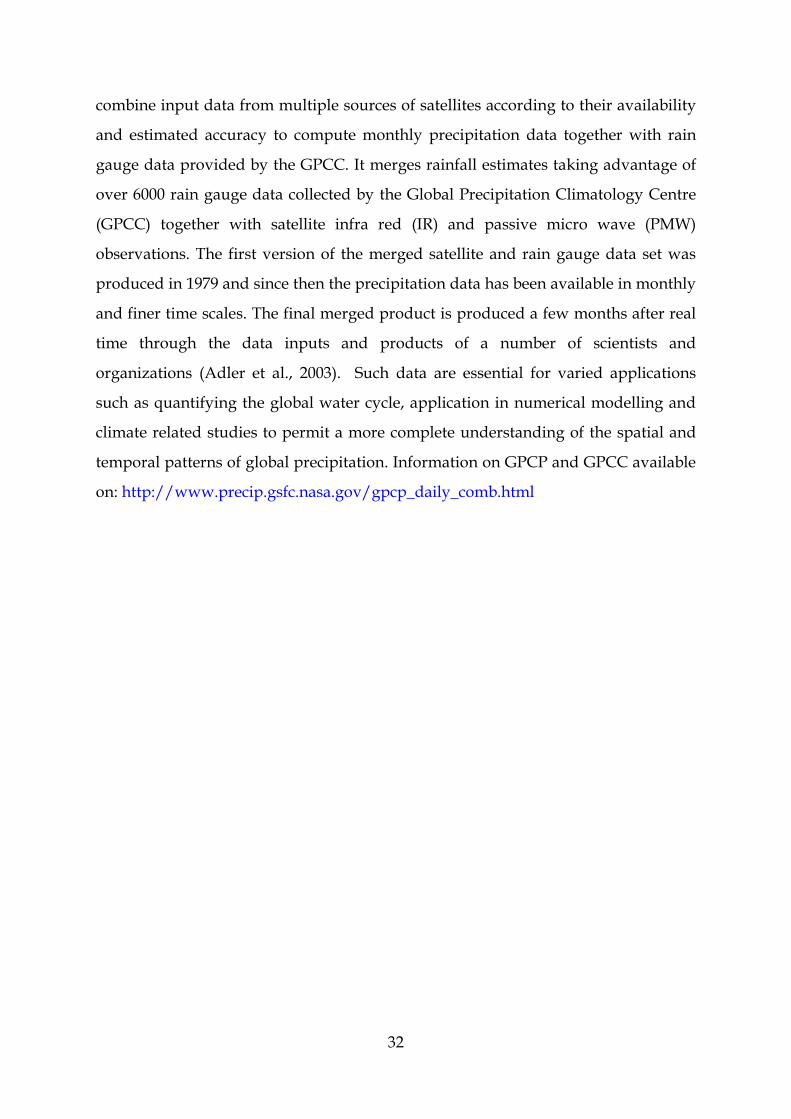
32

combine input data from multiple sources of satellites according to their availability

and estimated accuracy to compute monthly precipitation data together with rain

gauge data provided by the GPCC. It merges rainfall estimates taking advantage of

over 6000 rain gauge data collected by the Global Precipitation Climatology Centre

(GPCC) together with satellite infra red (IR) and passive micro wave (PMW)

observations. The first version of the merged satellite and rain gauge data set was

produced in 1979 and since then the precipitation data has been available in monthly

and finer time scales. The final merged product is produced a few months after real

time through the data inputs and products of a number of scientists and

organizations (Adler et al., 2003). Such data are essential for varied applications

such as quantifying the global water cycle, application in numerical modelling and

climate related studies to permit a more complete understanding of the spatial and

temporal patterns of global precipitation. Information on GPCP and GPCC available

on: http://www.precip.gsfc.nasa.gov/gpcp_daily_comb.html

33

5 DATA AND METHODOLOGY

This section describes the data and methodologies employed in data analysis

including different strategies applied in order to achieve the objectives of the study.

One intention of the study is to quantitatively evaluate the differences between the

three different rainfall estimates which are TAMSAT, GPCP and GPCC (gauge data)

including assessing the dependence of relative bias on seasonality and geographic

variations over southern Africa. Special interest will be on TAMSAT since it is also

widely available to all meteorological services in Southern Africa through the MSG

stations. The inter comparison focus on monthly, seasonal and annual scales using

data from January 1984 – December 2010. This period was chosen based on all three

datasets availability and completeness, especially TAMSAT data that is available

from 1983 (1983 omitted since data unstable at beginning). The strategy entailed

averaging the all datasets regionally and analysing the mean using different

statistical techniques such as differences in the mean, variation of the mean and

coefficient of variability.

Figure 5.1: Map showing zones used to compare rainfall estimates based on mean rainfall distribution in mm (1984-2010) over southern Africa. A (10 - 16°S, 14-40°E); B (16-25°S, 15-32°E); C (25-29°S, 18-31.5°E); D (29-33.5°S, 18-26°E); E (24-29°S, 27-31.5°E); F (16-25°S, 30-35.5°E)

34

Having identified the mean patterns of the rainfall distribution over Southern Africa,

the region was subdivided into smaller zones identified on basis of observed

prominent mean features during preliminary analysis and taking into consideration

the general climatic patterns over the region including mean topographic variations.

The method used in selecting the homogeneous zones is similar to the one used for

identifying calibration zones e.g. (Thorne et al., 2001) which depends on complexity

of regions rainfall characteristics which was also applied over southern Africa. Other

studies assessing satellite rainfall estimates such as Hong et al., (2007) and Hirpa et

al., (2010), also recommend that evaluation studies must take into consideration the

heterogeneity of the topography in addition to the specific region climatic

characteristics.

Southern Africa, unlike other parts of Africa such as northern Africa which has

generally invariant well defined fixed and documented climate zones cutting

through across country boundaries, has not been able to demarcate regional fixed

climatic zones. Over Southern Africa most studies on climate refer to weather

patterns (Manatsa et al., 2012; Blamey and Reason, 2012). This could be attributed to

the limited climate studies in the region besides the high spatial and temporal

rainfall variability, including the heterogeneity of the topography.

However, fixed zones are disadvantageous in regions such as southern Africa (sub-

tropics) with high rainfall variability where seasons with similar rainfall totals can

have quite diverse rainfall characteristics since the fixed zones are based on annual

rainfall totals and not rainfall generating patterns. This can be illustrated by for

example when convective storms of the ITCZ are the main source of rain which from

time to time does not arrive and retreat at the same time within the fixed climate

zone resulting in bias in the long term.

5.1 DATA

Three different gridded monthly data 1984 – 2010 were used for this assessment as

presented below. These data sets come in different grid resolution and it was

necessary to re-grid the data to a common grid scale for qualitative assessment and

35

comparison. Re-gridding is a process of interpolation from one grid resolution to a

different resolution. It entails converting the coordinates of each pixel into latitude

and longitude and calculating the mean of the variable of those pixel values falling

within that grid box of a particular longitude and latitude. For the comparison

between TAMSAT and GPCC data, the TAMSAT dataset was re-gridded to the

GPCC 0.5° x 0.5° grid box and to evaluate relation between TAMSAT and GPCP data

sets, the TAMSAT data re-gridded to the GPCP 2.5° x 2.5° grid boxes.

i) TAMSAT MONTHLY RAINFALL ESTIMATES

For this evaluation, the TAMSAT dataset which normally is at 0.0375° x 0.0375° grid

boxes was re- gridded to 0.5° x 0.5° grid resolution for comparison with GPCC

datasets by simple averaging over the appropriate number of pixels (Maidment et

al., 2012) and to 2.5° x 2.5° grid boxes for comparison with GPCP data.

ii) GPCC MONTHLY RAINFALL DATA

The GPCC version 6.0 data at 0.5° x 0.5° gridded monthly gauge data from 1984 –

2010 is used in the evaluation as the reference data. GPCC is a mature product that

has been widely applied on numerous precipitation related studies in similar fashion

to GPCP such as Ali et al., (2005), Layberry et al., (2006), Liebmann et al.,( 2012).

iii) GPCP MONTHLY RAINFALL DATA

Monthly GPCP version 2 data at 2.5° x 2.5 ° horizontal grid scale and calibrated in

degree daily (1DD) estimates (Xie et al., 2003) from 1984 – 2010 was used in the

evaluation. Similar to GPCC, this is a community based rainfall product which has

been used in a number of regional to continental scales precipitation studies e.g. (Xie

and Arkin, 1995; Hsu et al., 1997; Sorooshian et al., 2002; Huffman et al., 2001; Joyce

et al., 2004; Huffman et al., 2007; Bergès et al., 2010).

The availability of these datasets overcome data bureaucracies related to in country

data policies and promote data democracy, providing an efficient data service for

regional and global scientific studies such as this current study.

36

5.2 UNCERTAITY RELATED TO DATA GENERATION

From discussions in chapter 4 it can be understood that whether measured directly

by rain gauge or estimated by remote sensing technology, rainfall measurements,

hence data contain uncertainty. The estimation of the errors in both the gauges and

the satellite rainfall estimates can be a complex task which relates to the complexity

of techniques in use for rainfall estimation and measurements.

Rain gauges offer the simplest and direct method of rainfall measurement, but may

contain significant bias arising from poor spatial sampling, exposure of gauge and

aerodynamic effects especially during events with high intermittency such as

convection.

Remote sensed rainfall data involves indirect measurements and is inexact (Bell and

Kundu, 2003), hence quantitative use of satellite rainfall estimates require

information on accuracy of methodology. Rain rates vary remarkably with

topography resulting in rainfall gradients which satellites may not be measure

accurately as discussed above. This is especially an issue for polar orbiting satellite

based products (i.e. those based on MW data), which only pass over Africa twice a

day. Generally the uncertainty in the measurements between these systems can be

grouped into two main types viewed by many studies such as Adler et al., (2011).

i) SAMPLING ERROR OR RANDOM ERROR

This type of error consists of random measurements errors due to sampling

limitations and other related processes that also include variations in number of

gauges especially for combined satellite and gauge rainfall estimation techniques.

Random or sampling errors can be minimized by averaging over a large area and

over longer time period to guarantee stability of the samples.

ii) SYSTEMATIC ERROR

The systematic errors results from uncertainty in the measurement and related

sampling biases and the related algorithm. Uncertainties in satellite based rainfall

37

estimates are due to uncertainties in the retrieval processes as well as different

temporal and spatial sampling patterns of the observations systems. It has been

suggested by other writers such as Adler et al., (2011), that no amount of averaging

would eliminate systematic error and this usually forms part of the investigation in

inter-comparison exercises as is the cases presently. For gauge data, one cause of

systematic error could be gauge data continuously changing as gauging stations are

set up while others close down.

It becomes clear from the above discussion that full utilization of satellite-based

precipitation datasets may be hindered by the uncertainty and reliability associated

with the precipitation estimates.

5.3 METHODOLOGY

Comparison of the different rainfall estimates was performed using map plots and

different available statistical measures of describing datasets, dispersion amongst

datasets, evaluating agreement relations since it is difficult to find one standard

statistical measure with which to assess satellite rainfall estimation. For the purpose

of these study, will use simply relational measure, the root mean square error

(RMSE) and bias (b), mean absolute deviation and percentage difference (PDF). Each

of these different statistics only offers particular information about the errors being

evaluated hence the necessity to examine a number of statistical measures in

combination for a comprehensive picture of the error and bias. These statistical

indices have been extensively applied to evaluate relative accuracy of various

rainfall estimation products in other studies e.g. (Yilmaz et al., 2005, Ali et al., 2005,

Dinku et al., 2007, Adler et al., 2011, Jobard et al., 2011, Maidment et al., 2012). No

further assumptions are applied when using these statistics that may introduce

additional error.

Correlation co efficient (r) or relational measure is a single valued measure or degree

of association between two variables using a linear measure. Mathematically, the

correlation coefficient representation is as below, (symbols adopted relevant to the

study)

38

Correlation Coefficient (r) =

−

−−

=

−

∑ PPGG i

n

ii

1

������������

∑

−∑

−==

−− n

i

n

i

PPGG ii1

2

1

2 ... 5.1

Pi: ith satellite derived rainfall estimate; Gi: ith comparison data point. An over bar

represents the time-mean.

The correlation coefficient can be explained as the ratio of the sample covariance of

the two samples to the product of the two standard deviations (σ). The standard

deviation explains the clustering around the mean or amount of spread of the

dataset. Normally, for a leptokurtic bell shaped distribution, the standard deviation

is small and relatively large for skewed distributions (Wilks, 2011).

Sample standard deviation σ = ( )2

1

1∑

=

−n

iiX

Nµ ... 5.2

Where N is the sample size, Xi being the sample at point i, and µ being the sample

mean. Covariance describes the turbulence in the two variables while the standard

deviation, which is defined by the square-root of the variance, measures the spread

of the data about the mean which makes correlation to be sensitive to few outlier

point pairs. The variance describes the average of the squared differences from the

mean of the distribution. Correlation is bounded by, -1 ≤ R ≤ +1, thus for R = -1, a

perfect negative linear relationship exists between the variables, and if R = 1, a

perfect positive relation exists which is represented in a scatter plot by all points

falling in a straight line. Another property of the correlation coefficient is that R

squared (R2) explains the proportion of variance or variability of one of the two

variables that is linearly accounted for or described by the other. The major

weakness for correlation is that it does not account for bias which simple compares

the average magnitudes between the estimates in a form of a ratio as discussed

below.

39

Root mean squared error (RMSE) = � ( )∑ −=

n

iiiN

GP1

21 ... 5.3

The root mean squared error measures the average error magnitude. It should be

noted that because RMSE make use of the differences between the two estimated

values with one normally taken as reference, it gives more weight to larger error

magnitude which results from the squaring of the errors.

Bias or relative bias will be used to measure the correspondence between the

TAMSAT rainfall estimates and the GPCC and GPCP precipitation products. If one

product is consistently below or above (wet/dry) it exhibits bias regardless of its

relative accuracy or inaccuracy. One way of calculating bias or relative bias is use of

equation 5.4 below. Bias can be represented by percentage(s).

Percentage difference (PDF) or Relative bias = ∑=

−n

i i

ii

G

GP

1

... 5.4

The relative bias itself is useful in evaluating systematic errors of the satellite derived

rainfall estimates. Other available measures of bias which will be referred to from

time to time in the analysis include mean error which simply scales the average

difference between the rainfall estimates and observations, the mean absolute error

which computes the average magnitude of the error. Apart from correlation which

range between -1 and +1, ideal values for bias would be zero.

Additionally to the above discussed statistics, the Nash Sutcliffe Efficiency (NSI)

index will be used to compare the TAMSAT rainfall estimates against GPCC and

GPCP. This index determines the relative magnitude of the residual variance

compared to the variance of the ground observations, hence provides an indication

how well the plot of the observed estimation fits the bisector line (Thiemig et al.,

2012).

NSI = 1 -

( )

( )

−

−

∑

∑

=

=n

ii

n

iii

GG

GP

1

2

1

2

... 5.5

40

NSI can vary between -∞ and 1 and is not influenced by bias. Higher values of this

index (NSI =1) indicate better agreement between the simulated value and assumed

reference or observed value which in this case will be rainfall estimates. For NSI = 0,

the estimated values are as good as the observed mean, while for NSI < 0, indicates

that the observed mean is a better predictor than the estimator (Ali et al., 2005). Since

this skill score is composite of both linear association and bias, it is a better score to

other individual skill scores as was observed (Jobard et al., 2011).

Examining these estimates will provide a clear insight into the physical assumptions

in the product generation including impacts of the different strategies on the rainfall

estimation over southern Africa. Thus it is hoped that will also go a long way in

assisting the product developers with information required for appropriate action

based on the provided evidence. Similarly, the information derived from the

assessment would be helpful in applications and proper interpretation of the

different rainfall products to the different users hence improving confidence and

reliability of these products.

In general, the evaluation of these statistics is computed assuming an estimated

reference value. Most rainfall estimates inter-comparison studies (e.g. Thorne et al.

2001, Adler et al., 2011, Chadwick and Grimes, 2012, Roca et al., 2009, Maidment et

al., 2012) use gauge data as reference value and satellite rainfall product as the

estimated value, hence this evaluation will use GPCC and GPCP as reference values

and TAMSAT data as the estimated value.

Plotting, displaying and viewing the maps of the different rainfall estimates allow

straightforward visualization and evaluation (Yilmaz et al., 2005) of each rainfall

estimates which is essential in understanding and assessing the characteristics of

each rainfall datasets.

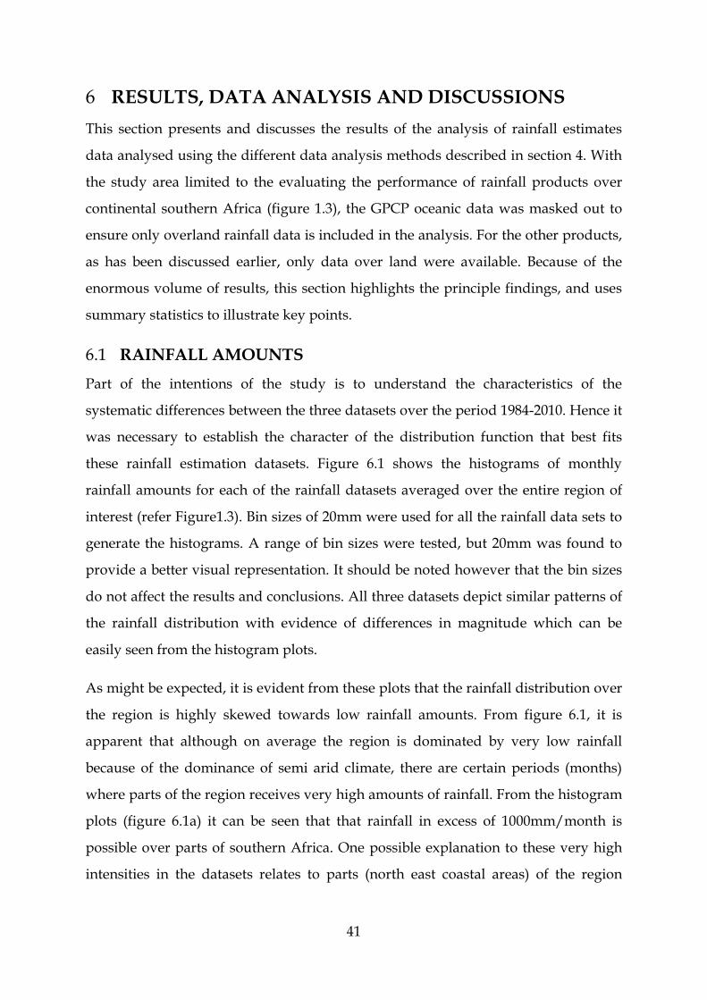
41

6 RESULTS, DATA ANALYSIS AND DISCUSSIONS

This section presents and discusses the results of the analysis of rainfall estimates

data analysed using the different data analysis methods described in section 4. With

the study area limited to the evaluating the performance of rainfall products over

continental southern Africa (figure 1.3), the GPCP oceanic data was masked out to

ensure only overland rainfall data is included in the analysis. For the other products,

as has been discussed earlier, only data over land were available. Because of the

enormous volume of results, this section highlights the principle findings, and uses

summary statistics to illustrate key points.

6.1 RAINFALL AMOUNTS

Part of the intentions of the study is to understand the characteristics of the

systematic differences between the three datasets over the period 1984-2010. Hence it

was necessary to establish the character of the distribution function that best fits

these rainfall estimation datasets. Figure 6.1 shows the histograms of monthly

rainfall amounts for each of the rainfall datasets averaged over the entire region of

interest (refer Figure1.3). Bin sizes of 20mm were used for all the rainfall data sets to

generate the histograms. A range of bin sizes were tested, but 20mm was found to

provide a better visual representation. It should be noted however that the bin sizes

do not affect the results and conclusions. All three datasets depict similar patterns of

the rainfall distribution with evidence of differences in magnitude which can be

easily seen from the histogram plots.

As might be expected, it is evident from these plots that the rainfall distribution over

the region is highly skewed towards low rainfall amounts. From figure 6.1, it is

apparent that although on average the region is dominated by very low rainfall

because of the dominance of semi arid climate, there are certain periods (months)

where parts of the region receives very high amounts of rainfall. From the histogram

plots (figure 6.1a) it can be seen that that rainfall in excess of 1000mm/month is

possible over parts of southern Africa. One possible explanation to these very high

intensities in the datasets relates to parts (north east coastal areas) of the region

42

occasionally being affected by tropical cyclones such as 1179mm in one month was

recorded over Southern Mozambique area (zone F, Figure 5.1) in February 2000

which coincides with tropical cyclone Eline.

Figure 6.1: Histograms of the three rainfall estimates over southern Africa 10°S, 35°S and 10°E, 40°E. (Figure 6.1a and 6.1b are at 0.5° x 0.5° while 6.1c and 6.1d are at 2.5° x 2.5° grid boxes)

Apart from the evidence from figure 6.1, the box plots in figure 6.2 also confirm the

skewness in these rainfall datasets. All the datasets show domination of outliers

beyond the top whisker which supports the understanding of high variability of the

climate of southern Africa as discussed in section 2 above, and in the published

literature (Jury et al., 2007).

These datasets are composed of very low median values, 19 mm for GPCC, 11mm

for TAMSAT at 0.5° grid scale, 26mm for GPCP and 9mm for TAMSAT at 2.5° grid

scale while the upper extreme values for all datasets are approximately 200 mm.

From the values presented above, TAMSAT estimates at the different grid scales are

lower compared to the other two datasets. From the summary of the descriptive

statistics, 25% of the rainfall lies between 0 - 3mm/month, and the mean ranges

43

between approximately 40 – 55mm/month. Unlike the median, the mean is highly

influenced by the occurrence of extreme rainfall events (large outliers) in the

datasets.

One other remarkable observation was that 75% of the time the region receives

approximately between 55–80mm/month, with extreme values range between

approximately 550–1280 mm/month, which shows high variability in rainfall in

time. The mean standard deviation for these datasets ranges between 25–

35mm/month which compares to the average of the datasets showing the extent of

variability in the rainfall estimates.

Figure 6.2: Diagram of box plots of the different rainfall estimation techniques during for period 1984-2010; (a) shows box plot of GPCC and TAMSAT rainfall estimates at 0.5° grid box, and (b) shows box plots of GPCP and TAMSAT rainfall estimates at 2.5° grid box

6.2 SPATIAL VARIATIONS

The large scale characteristics of the rainfall such as mean patterns, variability and

seasonality were evaluated at regional scale to allow for the stability of the

evaluation exercise as argued by Xie and Arkin, (1995) and at sub-regional scale to

reveal details that were obscured by smoothing at the regional scale. Figure 6.3

shows the mean rainfall map of the rainfall estimates from 1948-2010 over southern

44

Africa. Similar to the above plots, the three datasets have high similarity on the

distribution of rainfall over southern Africa and locating areas on high and low

rainfall estimates. These rainfall products however differ in the representation of the

magnitudes of the amounts of rainfall over the region. Figures 6.3a and 6.3b shows

map produced using GPCC and TAMSAT rainfall product at 0.5° x 0.5° grid

reference. Giving the benefit to GPCC as reference data (gauge data), these maps

show evidence of TAMSAT rainfall estimates generally being lower compared to the

GPCC rainfall products. Figures 6.3c and 6.3d represents GPCP and TAMSAT

rainfall estimates at 2.5° x 2.5° grid reference. Similarly, there is evidence of

TAMSAT rainfall estimates generally being lower than GPCP rainfall estimates.

These observed differences can be attributed to systematic difference in the

algorithms employed by these systems, including sampling limitations, orbital errors

and biases and other processes (see section 3) during data generation. In the GPCP

analysis procedure for example, there are adjustments (minimizing bias error) made

to satellite information using the GPCC gauge analysis over land and adjusting IR

estimates over the ocean by relatively less frequent by passive microwave estimates

(Adler et al., 2011). Though in the present case these datasets are in different grid

scales, it can be observed the strong relaxation towards the GPCC data by the GPCP

data showing that GPCP data are inevitably closer to GPCC than TAMSAT.

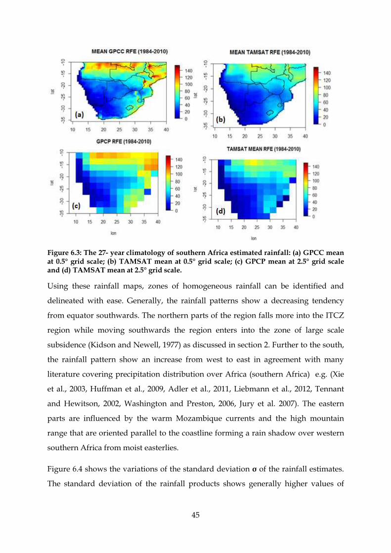
45

Figure 6.3: The 27- year climatology of southern Africa estimated rainfall: (a) GPCC mean at 0.5° grid scale; (b) TAMSAT mean at 0.5° grid scale; (c) GPCP mean at 2.5° grid scale and (d) TAMSAT mean at 2.5° grid scale.

Using these rainfall maps, zones of homogeneous rainfall can be identified and

delineated with ease. Generally, the rainfall patterns show a decreasing tendency

from equator southwards. The northern parts of the region falls more into the ITCZ

region while moving southwards the region enters into the zone of large scale

subsidence (Kidson and Newell, 1977) as discussed in section 2. Further to the south,

the rainfall pattern show an increase from west to east in agreement with many

literature covering precipitation distribution over Africa (southern Africa) e.g. (Xie

et al., 2003, Huffman et al., 2009, Adler et al., 2011, Liebmann et al., 2012, Tennant

and Hewitson, 2002, Washington and Preston, 2006, Jury et al. 2007). The eastern

parts are influenced by the warm Mozambique currents and the high mountain

range that are oriented parallel to the coastline forming a rain shadow over western

southern Africa from moist easterlies.

Figure 6.4 shows the variations of the standard deviation σ of the rainfall estimates.

The standard deviation of the rainfall products shows generally higher values of

46

standard deviation over areas with generally higher mean rainfall. Since rainfall is

non-Gaussian in nature (shown by the histograms of these datasets above) it is

expected that high standard deviation should coincide with generally high mean

rainfall. Higher values are found of the standard deviation are found over the north

eastern parts of southern Africa (central south Mozambique) which occasionally is

affected by tropical cyclones. Figures 6.4a and 6.4b represents GPCC and TAMSAT

rainfall product at 0.5° x 0.5° grid reference and these maps show evidence of

TAMSAT rainfall estimates generally lower compared to the GPCC rainfall

products, which can be expected considering that the standard deviation is closely

related to the mean of the distribution. Figures 6.4c and 6.4d represents GPCP and

TAMSAT rainfall estimates at 2.5° x 2.5° grid reference and similarly there is

evidence of TAMSAT rainfall estimates standard deviation being generally lower

than for GPCP.

Figure 6.4: The 27–year standard deviation climatology of rainfall over southern Africa rainfall: (a) GPCC mean at 0.5° grid scale; (b) TAMSAT mean at 0.5° grid scale; (c) GPCP mean at 2.5° grid scale and (d) TAMSAT mean at 2.5° grid scale.

47

Figure 6.5 provides an estimation of rainfall variability over southern Africa using

the coefficient of variation (CV) =µσ

, which is the ratio between the standard

deviation (σ) and the mean (µ) of the dataset. From these maps (Figure 6.5) it can be

observed that generally there is high variability over places with relatively low mean

rainfall and vice versa. Over the northern parts and along the eastern escarpment

areas of relatively high rainfall, the coefficient of variation ranges between (0.5 ≤ CV

≤ ~1) in all estimates compared to the central and western parts of the region. From

the definition of the coefficient of variation, such an observation can be expected,

indicating the bias related to this index. However, comparing TAMSAT and GPCC

coefficient of variation shows that TAMSAT has fewer areas with high variability

that GPCC. This could be attributed to the bias in TAMSAT representing extreme

high values which is evident from the box plots (Figure 6.2). For TAMSAT and

GPCP estimates however, there is an indication of greater variability in the TAMSAT

estimates than GPCP, which could be attributed to the high number of low rainfall

values in TAMSAT estimation as seen in the histogram plots (Figure 6.1c and d).

It should be noted however, that when the mean rainfall approaches zero, the

relative error become meaningless hence the standard deviation become a better

estimator. When the mean rainfall over an area is relatively large, the relative error

become much more meaningful to use and interpret.

48

Figure 6.5: The 27–year coefficient of variation of rainfall over southern Africa rainfall: (a) GPCC mean at 0.5° grid scale; (b) TAMSAT mean at 0.5° grid scale; (c) GPCP mean at 2.5° grid scale and (d) TAMSAT mean at 2.5° grid scale.

6.3 TEMPORAL VARIABILITY

Scatter plots of monthly precipitation for GPCC/GPCP against TAMSAT can be

used to compare monthly variations for the datasets, as discussed in section 5. Figure

6.6 shows the long term linear relationship between the datasets 1984-2010 and the

contribution of the different seasons (April – March and Sept – Aug) representing

dry and wet to the linear relationship. Generally, there is good correlation between

the pairs of rainfall estimates as can be seen from the scatter plots and the high

coefficient of determination (R2). The fitted regression line closely matches the

diagonal with a slight tilt away from TAMSAT estimates showing a dry bias by

TAMSAT estimation compared to the two other rainfall products.

One remarkable observation from the scatter plots is the contribution of the different

seasons to the linear relationship. It can be observed that different seasons contribute

differently to the linear relationship. During the dry season (figure 6.6c and 6.6d), it

49

can be observed the bias towards both GPCC and GPCP especially for relatively

high values which is also evident during the wet season.

Figure 6.6: Scatter plots of monthly rainfall (1984-2010) over southern Africa. (i) Red: (April – September), (ii) Green: (October – March). Note the different scales. Figure 6.6c and 6.6d are extracted from figure 6.6a and 6.6b for added for clarity. They only reveal / emphasize the red dots (dry months) below green (wet season) in 6.6a and 6.6b.

The scatter plots reveal adequately the limitations/capabilities of the different

methodologies in capturing very high values of precipitation as explained earlier. It

should be noted the contribution of averaging over time and large space

contribution to the observed generally high correlation amongst the estimates. The

agreement between GPCP and TAMSAT is slightly higher compared to GPCC and

TAMSAT estimation, which can be explained by both techniques use of IR

technology, though GPCP also incorporate gauge information and PMW to enhance

measurements performance which also increase bias between the two systems. This

can be seen during the winter months (figure 6.6d) when GPCP is able to measure

high values (values >400mm) which TAMSAT estimation is not able to detect. The

month to month variation in the relationship between the estimates is presented in

figure 6.7 confirming generally high R2 values >0.4 between Oct – April and lower

thereafter.

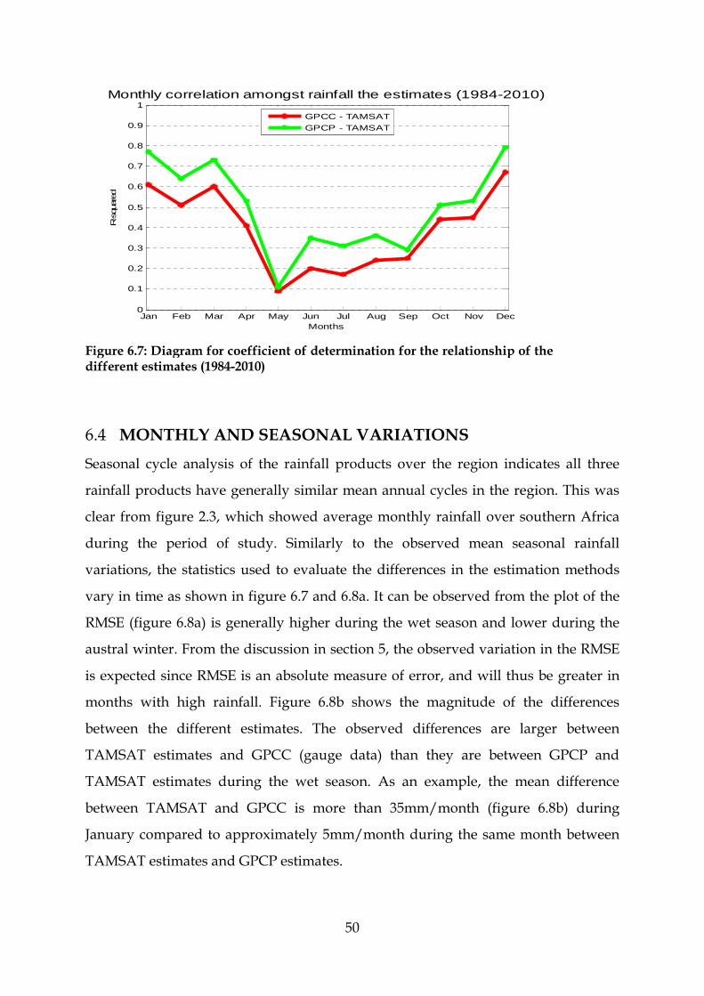
50

6.4 MONTHLY AND SEASONAL VARIATIONS

Seasonal cycle analysis of the rainfall products over the region indicates all three

rainfall products have generally similar mean annual cycles in the region. This was

clear from figure 2.3, which showed average monthly rainfall over southern Africa

during the period of study. Similarly to the observed mean seasonal rainfall

variations, the statistics used to evaluate the differences in the estimation methods

vary in time as shown in figure 6.7 and 6.8a. It can be observed from the plot of the

RMSE (figure 6.8a) is generally higher during the wet season and lower during the

austral winter. From the discussion in section 5, the observed variation in the RMSE

is expected since RMSE is an absolute measure of error, and will thus be greater in

months with high rainfall. Figure 6.8b shows the magnitude of the differences

between the different estimates. The observed differences are larger between

TAMSAT estimates and GPCC (gauge data) than they are between GPCP and

TAMSAT estimates during the wet season. As an example, the mean difference

between TAMSAT and GPCC is more than 35mm/month (figure 6.8b) during

January compared to approximately 5mm/month during the same month between

TAMSAT estimates and GPCP estimates.

Jan Feb Mar Apr May Jun Jul Aug Sep Oct Nov Dec0

0.1

0.2

0.3

0.4

0.5

0.6

0.7

0.8

0.9

1

Months

R-s

quar

ed

Monthly correlation amongst rainfall the estimates (1984-2010)

GPCC - TAMSAT

GPCP - TAMSAT

Figure 6.7: Diagram for coefficient of determination for the relationship of the different estimates (1984-2010)

51

Figure 6.8: Diagrams of variations in the comparison statistics. (a) Variations in the root mean square error of the mean for the different data sets. (b) Mean absolute differences in the datasets.

During the dry season, it was observed that there are generally larger differences

between the GPCP estimation and TAMSAT than there are during the wet months,

with TAMSAT being closer to the GPCC values which can be linked to the

contribution of the weather generating systems during the winter months and the

limitations and or capabilities of the different rainfall estimation techniques.

TAMSAT may be expected to estimate low rainfall during the austral winter. This is

because, during the austral winter, the major prevailing weather patterns and

contributing to rainfall (section 2) over much of southern Africa are the mid latitude

weather systems (frontal system) having varying strengths of baroclinicity. This can

result in convection or stratiform rainfall, characterised by warm clouds tops

unlikely to give rise to a signal that can be detected by an IR sensor hence the lower

estimation by the TAMSAT estimation technique (figure 4.1 TAMSAT

methodology), which is based on CCD and convection.

Another remarkable observation relates to the low difference between the satellite-

based rainfall estimates during the austral summer (GPCP and TAMSAT). During

DJF, the relative difference between GPCP and TAMSAT estimates is minimal (<

10%) compared to the relative difference between GPCC and TAMSAT estimates

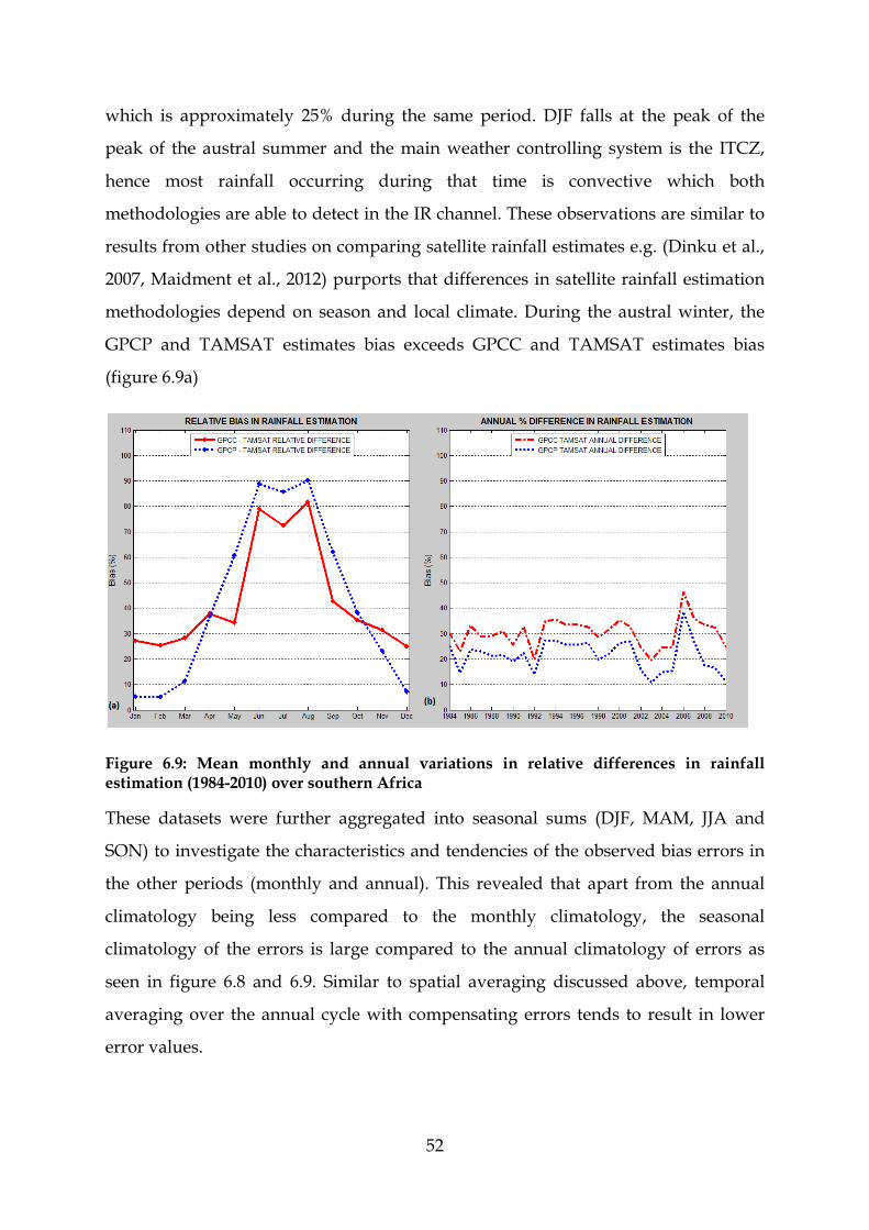
52

which is approximately 25% during the same period. DJF falls at the peak of the

peak of the austral summer and the main weather controlling system is the ITCZ,

hence most rainfall occurring during that time is convective which both

methodologies are able to detect in the IR channel. These observations are similar to

results from other studies on comparing satellite rainfall estimates e.g. (Dinku et al.,

2007, Maidment et al., 2012) purports that differences in satellite rainfall estimation

methodologies depend on season and local climate. During the austral winter, the

GPCP and TAMSAT estimates bias exceeds GPCC and TAMSAT estimates bias

(figure 6.9a)

Figure 6.9: Mean monthly and annual variations in relative differences in rainfall estimation (1984-2010) over southern Africa

These datasets were further aggregated into seasonal sums (DJF, MAM, JJA and

SON) to investigate the characteristics and tendencies of the observed bias errors in

the other periods (monthly and annual). This revealed that apart from the annual

climatology being less compared to the monthly climatology, the seasonal

climatology of the errors is large compared to the annual climatology of errors as

seen in figure 6.8 and 6.9. Similar to spatial averaging discussed above, temporal

averaging over the annual cycle with compensating errors tends to result in lower

error values.

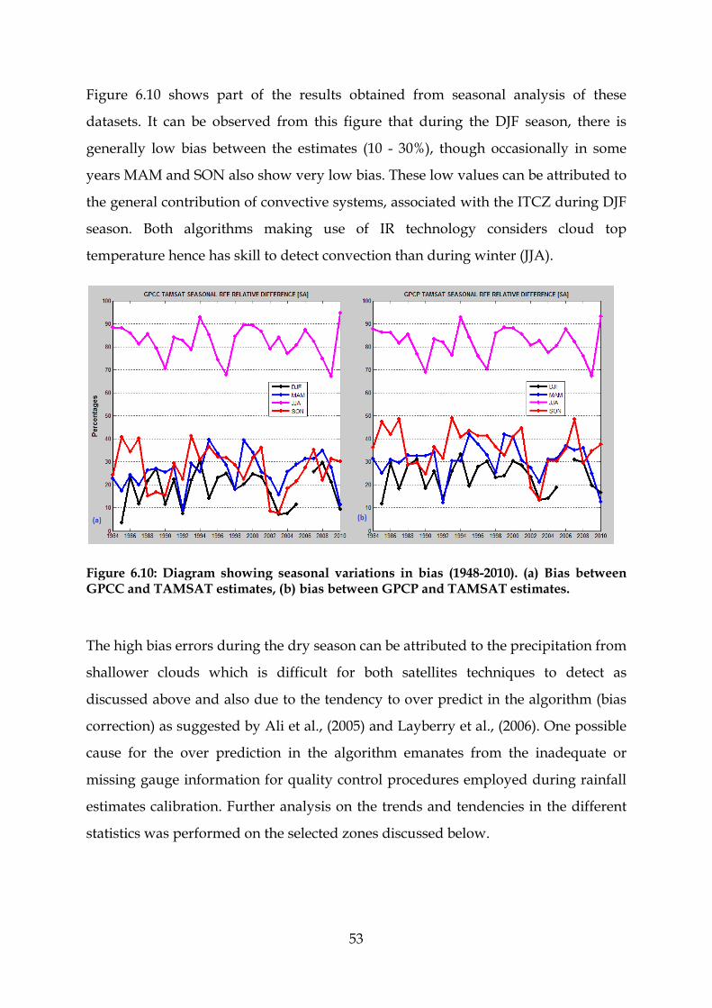
53

Figure 6.10 shows part of the results obtained from seasonal analysis of these

datasets. It can be observed from this figure that during the DJF season, there is

generally low bias between the estimates (10 - 30%), though occasionally in some

years MAM and SON also show very low bias. These low values can be attributed to

the general contribution of convective systems, associated with the ITCZ during DJF

season. Both algorithms making use of IR technology considers cloud top

temperature hence has skill to detect convection than during winter (JJA).

Figure 6.10: Diagram showing seasonal variations in bias (1948-2010). (a) Bias between GPCC and TAMSAT estimates, (b) bias between GPCP and TAMSAT estimates.

The high bias errors during the dry season can be attributed to the precipitation from

shallower clouds which is difficult for both satellites techniques to detect as

discussed above and also due to the tendency to over predict in the algorithm (bias

correction) as suggested by Ali et al., (2005) and Layberry et al., (2006). One possible

cause for the over prediction in the algorithm emanates from the inadequate or

missing gauge information for quality control procedures employed during rainfall

estimates calibration. Further analysis on the trends and tendencies in the different

statistics was performed on the selected zones discussed below.

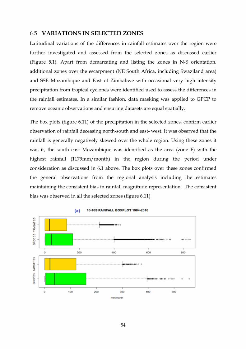
54

6.5 VARIATIONS IN SELECTED ZONES

Latitudinal variations of the differences in rainfall estimates over the region were

further investigated and assessed from the selected zones as discussed earlier

(Figure 5.1). Apart from demarcating and listing the zones in N-S orientation,

additional zones over the escarpment (NE South Africa, including Swaziland area)

and SSE Mozambique and East of Zimbabwe with occasional very high intensity

precipitation from tropical cyclones were identified used to assess the differences in

the rainfall estimates. In a similar fashion, data masking was applied to GPCP to

remove oceanic observations and ensuring datasets are equal spatially.

The box plots (figure 6.11) of the precipitation in the selected zones, confirm earlier

observation of rainfall deceasing north-south and east- west. It was observed that the

rainfall is generally negatively skewed over the whole region. Using these zones it

was it, the south east Mozambique was identified as the area (zone F) with the

highest rainfall (1179mm/month) in the region during the period under

consideration as discussed in 6.1 above. The box plots over these zones confirmed

the general observations from the regional analysis including the estimates

maintaining the consistent bias in rainfall magnitude representation. The consistent

bias was observed in all the selected zones (figure 6.11)

55

Figure 6.11: Diagram of box plots for different rainfall estimates over the selected zones. (a) Show box plot for the zone 10-16°S; (b) box plot for the zone 16-25°S, (c) for region 25-29°S and (d) represents region 29-33.5°S

56

Besides the strong seasonal variations in the associated differences (see previous

sections), there exist geographic variations in the error estimates which can be

observed from the summary statistics table 2 below. The geographic variations in the

rainfall estimates were easily represented by the root mean square error amongst the

estimates. The RMSE was found to be generally higher over areas with high rainfall

and lower over areas of low rainfall including being high during the wet season as

was observed earlier. Possible reasons were explained earlier 6.1 and 6.2 above. Zone

A and F had the highest root mean square error above 80% and these zones

generally have high rainfall since they are closer to the equator thus having great

influence from tropical air mass. However zone A showed R2 = 0.3 (amount of

information found in the rainfall relationship) between GPCC and TAMSAT

estimates. A number of factors can be thought of to contribute to the low R2 value;

hence low correlation. These include high rainfall variability indicated by existence

of large extreme rainfall values that are not detected by TAMSAT algorithm

(systematic bias). However, the possibility of the contribution of unavailability of

gauge information (figure 1.2) over this region is also likely another factor to the low

agreement between these datasets as discussed in section 5.

In general, high R2 values were observed between the rainfall products during the

summer months than during the dry season and the possible reason explained

above. The highest values of R2 = 0.5-0.6 corresponding to more than 50% of the

variance explained are found in zones B, C and D which are generally dry arid areas

with rainfall mainly from deep convection during summer. Low R2 of 0.2 was also

found between the rainfall estimates over the escarpment, which could be the result

of the nature of the common precipitation associated with orographic enhancement

and mid latitude weather systems influences. Similar results were obtained by

Thorne et al., (2001) showing very little change or improvement on the TAMSAT

methodology over this region since that study. During the austral summer months,

deep convection only contributes about 28% of the total monthly rainfall (Blamey

and Reason, 2012) over areas along the north east coast of south Africa, which

include the escarpment.

57

Discrepancies between the rainfall estimates are higher over areas indicated to have

no surface gauges information. Zone A has the highest bias (22%) during the austral

summer compared to 8% bias over the escarpment which is depicted having a fairy

dense network in figure 2. Systematic biases, amongst estimates can be reduced by

including gauge rainfall observations in the rainfall estimation model, as those

proposed by (Dybkjær, 2003), or a direct combination of the real-time rainfall

network observations (Grimes et al., 1999). Zone A is located in the region with no

gauges influencing concluding that the observed high bias over this zone is due to

unavailability of gauge information.

Table 6.1 Summary table of validation statistics for the different indices used in the comparison for the different seasons (winter and summer). Highest value to desired score for each category is highlighted

GPCC TAMSAT GPCP TAMSAT

Zone A Bias RMSE R2 NSI Bias RMSE R2 NSI

Summer 22.4 90.1 0.3 -2.4 23.0 70.7 0.5 -2.7

Winter 98.4 9.3 0.0 -4.5 98.7 8.9 0.0 -6.4

Zone B

Summer 8.0 50.1 0.6 0.5 15.1 40.7 0.7 0.2

Winter 89.3 5.6 0.2 -0.6 89.8 5.9 0.2 -1.0

Zone C

Summer 12.8 41.2 0.6 0.4 18.2 40.6 0.6 0.2

Winter 68.2 11.9 0.3 -0.0 76.9 14.5 0.4 -0.4

Zone D

Summer 14.7 24.3 0.5 0.3 31.2 28.9 0.6 0.0

Winter 64.1 30.6 0.1 -1.0 69.7 41.6 0.2 -1.5

Escarpment

Summer 8.5 54.1 0.2 0.2 11.5 47.7 0.4 0.2

Winter

Central Mozambique

Summer

Winter

80.8

23.2

98.4

16.4

87.7

22.2

0.3

0.5

0.1

-0.4

0.3

-2.1

84.4

19.4

97.9

17.0

67.1

18.9

0.4

0.6

0.1

-0.6

0.2

-2.9

58

Finally, the Nash Sutcliffe Index (NSI) was also used to test the skill of the different

estimates against each other. Generally, there was observed relatively good skill on

TAMSAT estimates following GPCC rainfall estimates during the rainy season

compared to the dry season similar to the other statistics. The closest agreement

between TAMSAT estimates and GPCC was found in zone B and C which is also

evident from the median values from box plots (figure 6.11b and c together with

high R2 (0.6) value. Similar to R2, the lowest skill score during summer is found in

zone A which is a possible confirmation of the effect of lack of gauge information on

the performance of the inter comparison exercise. Investigating the differences in

annual scales did not produce any significant different results from the monthly and

seasonal scales.

An R2 ≥ 0.4 over the region was found between TAMSAT and GPCP estimates

during the wet season. This indicates a good level of agreement in representing the

observed precipitation patterns which could be attributed to the common IR

sampling method and convection as discussed above. Besides both methodologies

utilizing the cloud top temperature and presence of convection during summer, it

should be noted that GPCP averages over a larger area (2.5° x 2.5° grid box) which

would smoothen random variations hence improving bias errors compared to

comparison between GPCC and TAMSAT (0.5 x 0.5° grid). Conversely, the observed

high relationship in summer become poor during the dry season, due to differences

in sampling methods capabilities or limitations and the representation of the general

prevailing climate as discussed above. The other statistics follow similar patterns

geographic and temporal patterns to the behaviour other measure between GPCC

and TAMSAT though with different magnitudes.

59

7 DISCUSSIONS AND CONCLUSIONS

This chapter provides discussions from the analysis and concludes the study. The

study provided a quantitative assessment of the characteristics, differences and

similarities in the three rainfall datasets generated using different measurement and

estimation techniques, to create an understanding of the characteristics, special

attributes, strengths and weaknesses of the different methodologies rainfall in

representation over southern Africa. A review of the main weather and climate

controlling systems over southern Africa was included to provide background

information on the mean patterns during the different seasons against which the

different rainfall measurement techniques were to be evaluated. Also the different

rainfall measurement methodologies were reviewed together with their known

uncertainties forming the basis to understand the resulting biases, tendencies, trends

and attributes from the data analysis.

Using descriptive statistical methodologies, the basic characteristics and probability

distribution functions best describing the GPCC, GPCP and TAMSAT rainfall

datasets were identified. The preliminary analysis revealed these datasets as highly

skewed (negative), indicating the high variability in the rainfall over the region. The

high variability in the rainfall was also confirmed by analysis of the mean and the

standard deviation of these rainfall estimates over the region. It was observed that

the standard deviation of the rainfall tracks or compares to the mean of the rainfall

which can be used to infer strong spread hence variability. Similarly, the analysis of

the coefficient of variability showed that areas with high variability coincide with

regions of relatively low monthly mean rainfall similar to suggestions in similar

studies, e.g. (Maidment et al., 2012).

The spatial analysis of the three datasets allowed identifying and selection of rainfall

homogeneous zones, which demonstrate the usefulness of global and satellite

derived rainfall in climate analysis. These identified climatic zones can be applied in

future climate studies.

60

The characteristics of the different rainfall datasets were evaluated over the selected

zones whose results proved that the estimates errors have both geographical and

temporal variations. Geographically the errors between GPCC and TAMSAT

estimates are higher (> 20%) to the northern parts of southern Africa where

availability of gauge information is poor as shown in figure 1.2. However, the errors

were generally minimal over the arid and generally flat regions (< 15%) of southern

Africa particularly during the austral summer period, similar to observations made

by (Thorne et al., 2001) in a TAMSAT comparison study over southern Africa. The

root mean square error was found to be higher over regions with high rainfall such

as > 80 mm over northern parts of southern Africa (Zone A) and relatively lower

over geographic regions with less rainfall, e.g. less than 25mm over south western

parts of southern Africa (zone D).

Seasonal variations amongst the bias errors were also identified exposing the

capabilities or limitations of the different measurements techniques. The annual plot

of the bias errors (figure 6.9b) indicate the bias errors becoming minimal coming

closer towards end of period which could be an indication of improvements in the

global and satellite rainfall estimation. This could be due to improved sensor

technology together with improvements in the algorithm e.g. (GPCC V6). However

these observed trend can only be confirmed in future validations.

Similar characteristics and observations of higher errors during the dry season

where even the correlation can be said to break down between GPCP and TAMSAT

rainfall estimates over certain geographical areas particularly over the extreme

southern tip of southern Africa were realised. This shows the limitations of IR cloud

top temperature based methodology during the cold season. The observed

geographical variations in the error were attributed to the variations or intermittency

of the weather systems and the topography, together with systematic bias of the

different rainfall measurement techniques.

From the analysis and these discussions the characteristics of the different rainfall

estimates in space and over time can be understood. These rainfall estimates

61

generally compare well to each other especially during the summer season and over

certain regions with distinct topographic and climatic features. The differences

amongst the different methodologies are persistent and stable over time as shown in

(figure 6.9b). As discussed above, it becomes apparent that the TAMSAT rainfall

estimates are generally lower in representation of magnitude of rainfall amounts, but

generally in agreement in terms of structure to GPCC and GPCP in estimating and

representing the mean rainfall over much of southern Africa. Variations in errors

highlight the deficiencies of satellite rainfall algorithms for estimating spatially and

temporally variable rainfall. Considering the observed differences in the rainfall

magnitude amongst the rainfall estimates, it would be desirable to understand the

effect of these differences in other climate related studies.

(i) RECOMMENDATIONS

To improve on the effect of the systematic biases, near real time gauges or a direct

combination of near real time rainfall observations should be included in the

TAMSAT methodology, as those proposed by (Grimes et al., 1999). It is however

worth noting that this suggestion will not be without challenges especially in regions

where the gauge network is sparse. Augmentation of availability of gauge data can

be possible through participation of local meteorological and hydrological services

in regular validation e.g. (multiannual time scale) exercises which also assist

improving understanding, applicability and visibility of satellite derived rainfall

estimates. Understanding the operational accuracy requirements for satellite rainfall

estimates would offer an additional incentive to the local national meteorological

and hydrological services to invest on improving the local rain gauge networks and

exchange available gauge data with the global centres.

Alternatively, a basic satellite rain gauge calibration network capable of automatic or

self calibration can be established in partnership and collaboration with the local

meteorological and hydrological services and the satellite data providers over

idealised locations considering that the rain gauge network has been observed to be

declining with little hope for improvements over Africa region. This can be extended

62

and developed from existing data collecting platforms (DCP) technology with GPS

capabilities.

(ii) LIMITATIONS

The study was limited to monthly rainfall data analysis, thus only monthly time

scales and beyond were possible in the analysis. Noting the importance of rainfall

over the region and the high reliance of agriculture production and water resources

on rainfall, shorter time scales (dekad) of rainfall analysis have a wider application.

The study confirmed that the rainfall over southern Africa is characterised by high

spatial and temporal variability in nature which leads to high vulnerability when the

rainfall departs from the expected or normal patterns.

GTS derived gauge data (GPCC) was utilised as reference data for the study, which

is not easy to establish the exact number and location of the gauge source that went

into the rainfall data generation. It is understood and was shown (figure 1.2) that the

region suffers from uneven distribution of gauge network and uncertainty on

rainfall estimates depends strongly on gauge network density as was discussed. A

weak correlation between the TAMSAT and GPCC estimates was observed over

zone A (figure 5.1) which apart from attributing this to systematic errors and

random variability in the climate system provides reason for bias towards effects of

lack of gauge information. The unavailability of gauge information within each grid

box made it not possible geo referencing of the satellite derived estimates to ensure

that all satellite pixel information on the data is positioned over the correct

geographic location on the earth’s surface. However, none of the observations

showed obvious signs of misrepresentation of the rainfall over the region.

(iii) FUTURE WORK

Noting the results of the study, further studies are desirable to consider improving

or optimising the accuracy of TAMSAT rainfall estimates by correcting for bias error

using localised rain gauge measurements. From the consistency in the bias errors

63

over time, it is likely to fit a model for bias correction or optimisation of the

TAMSAT rainfall estimates.

Also noting that the satellite rainfall estimates represent the mean rainfall over the

region with good skill, future work should consider also investigating

characterization of inter and intra seasonal rainfall variability utilizing satellite

derived rainfall estimates such as onset, cessation of rainfall and variability over the

region.

As mentioned in the recommendations, other relevant studies to satellite rainfall

estimates should consider optimal rainfall calibration network over Africa for

satellite rainfall estimates optimization and bias correction.

64

BIBLIOGRAPHY

Adler, R.F., Gu, G., Huffman, G.J., 2011. Estimating Climatological Bias Errors for the Global Precipitation Climatology Project (GPCP). J. Appl. Meteorol. Clim. 51, 84–99.

Adler, R.F., Huffman, G.J., Chang, A., Ferraro, R., Xie, P.-P., Janowiak, J., Rudolf, B., Schneider, U., Curtis, S., Bolvin, D., Gruber, A., Susskind, J., Arkin, P., Nelkin, E., 2003. The Version-2 Global Precipitation Climatology Project (GPCP) Monthly Precipitation Analysis (1979–Present). J. Hydrometeorol. 4, 1147–1167.

Adler, R.F., Negri, A.J., 1988. A Satellite Infrared Technique to Estimate Tropical Convective and Stratiform Rainfall. J. Appl. Meteorol. 27, 30–51.

Ali, A., Amani, A., Diedhiou, A., Lebel, T., 2005. Rainfall estimation in the Sahel. Part II: Evaluation of rain gauge networks in the CILSS countries and objective intercomparison of rainfall products. J. Appl. Meteorol. 44, 1707–1722.

Annamalai, H., Murtugudde, R., 2004. Role of the Indian Ocean in Regional Climate Variability, in: Wang, C., Xie, S.P., Carton, J.A. (Eds.), Earth’s Climate. American Geophysical Union, pp. 213–246.

Arkin, P.A., Meisner, B.N., 1987. The Relationship between Large-Scale Convective Rainfall and Cold Cloud over the Western Hemisphere during 1982-84. Mon. Weather Rev. 115, 51–74.

Arnell, N., 2002. Hydrology and Global Environmental Change. Pearson Education. Bell, T.L., Kundu, P.K., 2003. Comparing satellite rainfall estimates with rain gauge

data: Optimal strategies suggested by a spectral model. J. Geophys. Res. Atmospheres 108.

Bellerby, T.J., Sun, J., 2005. Probabilistic and Ensemble Representations of the Uncertainty in an IR/Microwave Satellite Precipitation Product. J. Hydrometeorol. 6, 1032–1044.

Bergès, J.C., Jobard, I., Chopin, F., Roca, R., 2010. EPSAT-SG: a satellite method for precipitation estimation; its concepts and implementation for the AMMA experiment. Ann Geophys 28, 289–308.

Blamey, R.C., Reason, C.J.C., 2012. The Role of Mesoscale Convective Complexes in Southern Africa Summer Rainfall. J. Clim. 26, 1654–1668.

Boko, M., Niang, I., Nyong, A., Vogel, C., Githeko, A., Medany, M., Osman-Elasha, B., Tabo, R., Yanda, P., 2007. Africa.

CCAFS, 2012. CCAFS Technical Report - May 2012.pdf CCAFS: Rainfall Data Generation and Analysis for African Meteorology Technical Report [Grimes et al], (May 2012).

CCAFS,, 2012. CCAFS: Rainfall Data Generation and Analysis for African Meteorology Final Technical Report, [Shine et al], (July 2012).

Chadwick, R., Grimes, D., 2012. An Artificial Neural Network Approach to Multispectral Rainfall Estimation over Africa. J. Hydrometeorol. 13, 913–931.

Chikoore, H., Jury, M.R., 2010. Intraseasonal Variability of Satellite-Derived Rainfall and Vegetation over Southern Africa. Earth Interactions 14, 1–26.

65

Cook, C., Reason, C.J.C., Hewitson, B.C., 2004. Wet and dry spells within particularly wet and dry summers in the South African summer rainfall region. Clim. Res. 26, 17–31.

Curran, P., 1982. The use of satellite data in rainfall monitoring. E. C. Barrett and W. M. Martin, Academic Press, London, 1981. No. of pages: 340. Price: £27.80. J. Clim. 2, 198–198.

De Coning, E., Poolman, E., 2011. South African Weather Service operational satellite based precipitation estimation technique: applications and improvements. Hydrol Earth Syst Sci 15, 1131–1145.

Dinku, T., Ceccato, P., Grover‐Kopec, E., Lemma, M., Connor, S., Ropelewski, C., 2007. Validation of satellite rainfall products over East Africa’s complex topography. Int. J. Remote Sens. 28, 1503–1526.

Dybkjær, G., 2003. A simple self-calibrating cold cloud duration technique applied in West Africa and Bangladesh. Geogr. Tidsskr.-Dan. J. Geogr. 103, 83–97.

Fauchereau, N., Pohl, B., Reason, C.J.C., Rouault, M., Richard, Y., 2009. Recurrent daily OLR patterns in the Southern Africa/Southwest Indian Ocean region, implications for South African rainfall and teleconnections. Clim. Dyn. 32, 575–591.

Golnaraghi, M., Douris, J., Migraine, J.B., 2009. Saving lives through early warning systems and emergency preparedness. Risk Wise 137–141.

Gosset, M., Viarre, J., Quantin, G., Alcoba, M., 2013. Evaluation of several rainfall products used for hydrological applications over West Africa using two high-resolution gauge networks. Q. J. R. Meteorol. Soc.

Grimes, D.I.., Pardo-Igúzquiza, E., Bonifacio, R., 1999. Optimal areal rainfall estimation using raingauges and satellite data. J. Hydrol. 222, 93–108.

GRIMES, D.I.F., DIOP, M., 2003. Satellite-based rainfall estimation for river flow forecasting in Africa. I: Rainfall estimates and hydrological forecasts. Hydrol. Sci. J. 48, 567–584.

Habib, E., Krajewski, W., Kruger, A., 2001. Sampling Errors of Tipping-Bucket Rain Gauge Measurements. J. Hydrol. Eng. 6, 159–166.

Herman, A., Kumar, V.B., Arkin, P.A., Kousky, J.V., 1997. Objectively determined 10-day African rainfall estimates created for famine early warning systems. Int. J. Remote Sens. 18, 2147–2159.

Hirpa, F.A., Gebremichael, M., Over, T.M., 2010. River flow fluctuation analysis: Effect of watershed area. Water Resour. Res. 46,.

Holloway, A., 2003. Disaster risk reduction in southern Africa: hot rhetoric—cold reality. Afr. Secur. Stud. 12, 29–38.

Hong, G., Yang, P., Huang, H.-L., Baum, B.A., Hu, Y., Platnick, S., 2007. The Sensitivity of Ice Cloud Optical and Microphysical Passive Satellite Retrievals to Cloud Geometrical Thickness. IEEE Trans. Geosci. Remote Sens. 45, 1315–1323.

Hsu, K., Gao, X., Sorooshian, S., Gupta, H.V., 1997. Precipitation Estimation from Remotely Sensed Information Using Artificial Neural Networks. J. Appl. Meteorol. 36, 1176–1190.

66

Huffman, G.J., Adler, R.F., Bolvin, D.T., Gu, G., 2009. Improving the global precipitation record: GPCP Version 2.1. Geophys. Res. Lett. 36.

Huffman, G.J., Adler, R.F., Morrissey, M.M., Bolvin, D.T., Curtis, S., Joyce, R., McGavock, B., Susskind, J., 2001. Global Precipitation at One-Degree Daily Resolution from Multisatellite Observations. J. Hydrometeorol. 2, 36–50.

Huffman, G.J., Adler, R.F., Rudolf, B., Schneider, U., Keehn, P.R., 1995. Global Precipitation Estimates Based on a Technique for Combining Satellite-Based Estimates, Rain Gauge Analysis, and NWP Model Precipitation Information. J. Clim. 8, 1284–1295.

Huffman, G.J., Bolvin, D.T., Nelkin, E.J., Wolff, D.B., Adler, R.F., Gu, G., Hong, Y., Bowman, K.P., Stocker, E.F., 2007. The TRMM Multisatellite Precipitation Analysis (TMPA): Quasi-Global, Multiyear, Combined-Sensor Precipitation Estimates at Fine Scales. J. Hydrometeorol. 8, 38–55.

IPCC, 2007c, 2007. Climate change 2007: impacts, adaptation and vulnerability. Contrib. Work. Group II Fourth Assess. Rep. Intergov. Panel Clim. Change Camb. Univ. Press Camb. UK.

Janowiak, J.E., 1988. An Investigation of Interannual Rainfall Variability in Africa. J. Clim. 1, 240–255.

Jobard, I., Chopin, F., Berges, J.C., Roca, R., 2011. An intercomparison of 10-day satellite precipitation products during West African monsoon. Int. J. Remote Sens. 32, 2353–2376.

Joyce, R.J., Janowiak, J.E., Arkin, P.A., Xie, P., 2004. CMORPH: A method that produces global precipitation estimates from passive microwave and infrared data at high spatial and temporal resolution. J. Hydrometeorol. 5, 487–503.

Jury, M., Rautenbach, H., Tadross, M., Philipp, A., 2007. Evaluating spatial scales of climate variability in sub-Saharan Africa. Theor. Appl. Clim. 88, 169–177.

Jury, M.R., Enfield, D.B., Mélice, J.-L., 2002. Tropical monsoons around Africa: Stability of El Niño–Southern Oscillation associations and links with continental climate. J. Geophys. Res. Oceans 107, 15–1–15–17.

Kidson, J.W., Newell, R.E., 1977. African rainfall and its relation to the upper air circulation. Q. J. R. Meteorol. Soc. 103, 441–456.

Kummerow, C., Hong, Y., Olson, W.S., Yang, S., Adler, R.F., McCollum, J., Ferraro, R., Petty, G., Shin, D.-B., Wilheit, T.T., 2001. The Evolution of the Goddard Profiling Algorithm (GPROF) for Rainfall Estimation from Passive Microwave Sensors. J. Appl. Meteorol. 40, 1801–1820.

Layberry, R., Kniveton, D.R., Todd, M.C., Kidd, C., Bellerby, T.J., 2006. Daily precipitation over southern Africa: A new resource for climate studies. J. Hydrometeorol. 7, 149–159.

Liebmann, B., Bladé, I., Kiladis, G.N., Carvalho, L.M.V., B. Senay, G., Allured, D., Leroux, S., Funk, C., 2012. Seasonality of African Precipitation from 1996 to 2009. J. Clim. 25, 4304–4322.

Lillesand, T.M., Kiefer, R.W., Chipman, J.W., 2004. Remote sensing and image interpretation. John Wiley & Sons Ltd.

Lindesay, J., Bridgman, H.A., 1998. Climates of the southern continents: present, past, and future. Wiley.

67

Lindesay, J.A., Vogel, C.H., 1990. Historical evidence for Southern Oscillation-southern African rainfall relationships. Int. J. Clim. 10, 679–689.

Maidment, R.I., Grimes, D.I.F., Allan, R.P., Greatrex, H., Rojas, O., Leo, O., 2012. Evaluation of satellite-based and model re-analysis rainfall estimates for Uganda. Meteorol. Appl..

Manatsa, D., Reason, C.J.C., Mukwada, G., 2012. On the decoupling of the IODZM from southern Africa Summer rainfall variability. Int. J. Clim. 32, 727–746.

Mason, S.J., Goddard, L., 2001. Probabilistic Precipitation Anomalies Associated with ENSO. Bull. Am. Meteorol. Soc. 82, 619–638.

Meehl, G.A., Stocker, T.F., Collins, W.D., Friedlingstein, P., Gaye, A.T., Gregory, J.M., Kitoh, A., Knutti, R., Murphy, J.M., Noda, A., 2007. et al. 2007 Global climate projections. Clim. Change 2007 Phys. Sci. Basis Contrib. Work. Group Fourth Assess. Rep. Intergov. Panel Clim. Change 747–846.

Milford, J.R., McDougall, V.D., Dugdale, G., 1994. Rainfall estimation from cold cloud duration, experience of the TAMSAT group in West Africa, in: Validation Problems of Rainfall Estimation by Satellite in Intertropical Africa, Guillot B., Edt., Proc. Niamey Workshop. pp. 1–3.

Morin, E., Maddox, R.A., Goodrich, D.C., Sorooshian, S., 2005. Radar Z – R Relationship for Summer Monsoon Storms in Arizona. Weather Forecast. 20, 672–679.

Ogallo, L., 2010. The Mainstreaming of Climate Change and Variability Information into Planning and Policy Development for Africa. Procedia Environ. Sci. 1, 405 – 410.

Owolawi, P.A., 2011. Rainfall Rate Probability Density Evaluation and Mapping for the Estimation of Rain Attenuation in South Africa and Surrounding Islands. Prog. Electromagn. Res.-Pier 112, 155–181.

Pierre, C., Bergametti, G., Marticorena, B., Mougin, E., Lebel, T., Ali, A., 2011. Pluriannual comparisons of satellite-based rainfall products over the Sahelian belt for seasonal vegetation modeling. J. Geophys. Res. Atmospheres 116.

Preston-Whyte, R.A., Tyson, P.D., 1988. The Atmosphere and Weather of Southern Africa. Oxford University Press, South Africa.

Reason, C. j. c., Rouault, M., 2002. ENSO-like decadal variability and South African rainfall. Geophys. Res. Lett. 29, 16–1–16–4.

Reason, C.J.C., Jagadheesha, D., 2005. A model investigation of recent ENSO impacts over southern Africa. Meteorol. Atmospheric Phys. 89, 181–205.

Reason, C.J.C., Landman, W., Tennant, W., 2006. Seasonal to Decadal Prediction of Southern African Climate and Its Links with Variability of the Atlantic Ocean. Bull. Am. Meteorol. Soc. 87, 941–955.

Richard, Y., Trzaska, S., Roucou, P., Rouault, M., 2000. Modification of the southern African rainfall variability/ENSO relationship since the late 1960s. Clim. Dyn. 16, 883–895.

Roca, R., Chambon, P., Jobard, I., Kirstetter, P.-E., Gosset, M., Bergès, J.C., 2009. Comparing Satellite and Surface Rainfall Products over West Africa at Meteorologically Relevant Scales during the AMMA Campaign Using Error Estimates. J. Appl. Meteorol. Clim. 49, 715–731.

68

Roca, R., Chambon, P., Jobard, I., Kirstetter, P.-E., Gosset, M., Bergès, J.C., 2010. Comparing Satellite and Surface Rainfall Products over West Africa at Meteorologically Relevant Scales during the AMMA Campaign Using Error Estimates. J. Appl. Meteorol. Clim. 49, 715–731.

Romilly, T.G., Gebremichael, M., 2011. Evaluation of satellite rainfall estimates over Ethiopian river basins. Hydrol Earth Syst Sci 15, 1505–1514.

Ropelewski, C.F., Halpert, M.S., 1987. Global and Regional Scale Precipitation Patterns Associated with the El Niño/Southern Oscillation. Mon. Weather Rev. 115, 1606–1626.

Ropelewski, C.F., Halpert, M.S., 1989. Precipitation Patterns Associated with the High Index Phase of the Southern Oscillation. J. Clim. 2, 268–284.

Rouault, M., Richard, Y., 2005. Intensity and spatial extent of droughts in southern Africa. Geophys. Res. Lett. 32.

SADC,2010,Southern_Africa_Framework_of_Subregional_Climate_Change_Programes, (2011-2015).

Saji, N.H., Goswami, B.N., Vinayachandran, P.N., Yamagata, T., 1999. A dipole mode in the tropical Indian Ocean. Nature 401, 360–363.

Sawunyama, T., Hughes, D.A., 2008. Application of satellite-derived rainfall estimates to extend water resource simulation modelling in South Africa. Water SA 34, 1–9.

Schneider, U., Fuchs, T., Meyer-Christoffer, A., Rudolf, B., 2008. Global precipitation analysis products of the GPCC. Glob. Precip. Clim. Cent. GPCC DWD Internet Publ. 1–12.

Song, Q., Vecchi, G.A., Rosati, A.J., 2008. Predictability of the Indian Ocean sea surface temperature anomalies in the GFDL coupled model. Geophys. Res. Lett. 35.

Sorooshian, S., Gao, X., Hsu, K., Maddox, R.A., Hong, Y., Gupta, H.V., Imam, B., 2002. Diurnal Variability of Tropical Rainfall Retrieved from Combined GOES and TRMM Satellite Information. J. Clim. 15, 983–1001.

Stephens, G.L., Kummerow, C.D., 2007. The Remote Sensing of Clouds and Precipitation from Space: A Review. J. Atmospheric Sci. 64, 3742–3765.

Strangeways, I., 2007. Precipitation: Theory, Measurement and Distribution, Precipitation: Theory, Measurement and Distribution. Cambridge University Press.

Tennant, W.J., Hewitson, B.C., 2002. Intra-seasonal rainfall characteristics and their importance to the seasonal prediction problem. Int. J. Clim. 22, 1033–1048.

Thiemig, V., Rojas, R., Zambrano-Bigiarini, M., Levizzani, V., De Roo, A., 2012. Validation of Satellite-Based Precipitation Products over Sparsely Gauged African River Basins. J. Hydrometeorol. 13, 1760–1783.

Thorne, V., Coakeley, P., Grimes, D., Dugdale, G., 2001. Comparison of TAMSAT and CPC rainfall estimates with raingauges, for southern Africa. Int. J. Remote Sens. 22, 1951–1974.

Trenberth, K.E., Smith, L., Qian, T., Dai, A., Fasullo, J., 2007. Estimates of the Global Water Budget and Its Annual Cycle Using Observational and Model Data. J. Hydrometeorol. 8, 758–769.

69

Washington, R., Kay, G., Harrison, M., Conway, D., Black, E., Challinor, A., Grimes, D., Jones, R., Morse, A., Todd, M., 2006. African Climate Change: Taking the Shorter Route. Bull. Am. Meteorol. Soc. 87, 1355–1366.

Washington, R., Preston, A., 2006. Extreme wet years over southern Africa: Role of Indian Ocean sea surface temperatures. J. Geophys. Res. Atmospheres 111, D15104.

Wilks, 2011. Statistical Methods in the Atmospheric Sciences (Hardback), 3, Revised. ed.

WIND, 2011. Weather INformation for Development (WIND) [Vicky Easterbrook] Accenture Development Partnerships (ADP) 22 February 2011.

Xie, P., Arkin, P.A., 1995. An Intercomparison of Gauge Observations and Satellite Estimates of Monthly Precipitation. J. Appl. Meteorol. 34, 1143–1160.

Xie, P., Janowiak, J.E., Arkin, P.A., Adler, R., Gruber, A., Ferraro, R., Huffman, G.J., Curtis, S., 2003. GPCP Pentad Precipitation Analyses: An Experimental Dataset Based on Gauge Observations and Satellite Estimates. J. Clim. 16, 2197–2214.

Yilmaz, K.K., Hogue, T.S., Hsu, K., Sorooshian, S., Gupta, H.V., Wagener, T., 2005. Intercomparison of Rain Gauge, Radar, and Satellite-Based Precipitation Estimates with Emphasis on Hydrologic Forecasting. J. Hydrometeorol. 6, 497–517.

Yong, B., Ren, L.-L., Hong, Y., Chen, X., Wang, W., Li, Q., Yuan, F., 2010. Inter-comparison of two standard satellite-based precipitation products at basin scale.

Zahn, M., Allan, R.P., 2013. Climate Warming–Related Strengthening of the Tropical Hydrological Cycle. J. Clim. 26, 562–574.

http://www.ncdc.noaa.gov [10 July, 2013]

http://www.eumetsat.int [18 July, 2013]

http://www.ospo.noaa.gov [ 10 July, 2013]

http://www.precip.gsfc.nasa.gov/gpcp_daily_comb.html [26 June, 2013]

http://www.wmo.int/pages/prog/drr/ [ 06 June, 2013]