Embed Size (px)
Citation preview
School of Chemical TechnologyDegree Programme of Chemical Technology
Henrik Heino
Particle movement and mixing in three-phase gas-liquid-solidfluidized bed
Master’s thesis for the degree of Master of Science in Technologysubmitted for inspection, Espoo, 10 November, 2015.
Supervisor Professor Ville Alopaeus
Instructor M.Sc. Olli Sorvari

Aalto University, P.O. BOX 11000, 00076 AALTOwww.aalto.fi
Abstract of master's thesis
I
Author Henrik Heino
Title of thesis Particle movement and mixing in three-phase gas-liquid-solidfluidized bed
Department Department of Biotechnology and Chemical Technology
Professorship Chemical Engineering Code of professorship KE-42
Thesis supervisor Prof. Ville Alopaeus
Thesis advisor(s) / Thesis examiner(s) M.Sc. (Tech.) Olli Sorvari
Date 10.11.2015 Number of pages 83 Language English
AbstractThe objective of this thesis is to study the movement and the mixing of the particlesin the liquid-solid and the gas-liquid-solid fluidization as well as to provide validationdata of the fluidized bed behavior. The results are used for validation in CFD(computational fluid dynamics) models at a concurrent PhD thesis.The experiments were made in a rectangular 10 cm by 10 cm column. The used liquidand gas phases in the experiments were tap water and compressed air, respectively.The solid particles in the fluidized bed were 2.3 mm diameter glass beads. Theexperiments were carried out varying the flow rates of the gas and liquid entering thecolumn. The bed height, the pressure difference in the bed, the superficial flowvelocities of the gas and the liquid, and the particle movement patterns were observedand measured during the experiments. The particle movement and the bubble flowregimes were analyzed from video recording.
In the experiments the minimum fluidization points at the different superficial gasvelocities were measured. In addition, the solid and the gas-hold-up as well as thebed expansion were calculated from the measurements for different superficial gasand liquid flow velocities.
It was found out that superficial liquid velocity at minimum fluidization point ishigher with zero or diminutive gas flow than when the gas flow is larger. In addition,when superficial gas flow is larger the superficial liquid velocity at minimumfluidization point is independent on gas flow rate. It was found that the bed expansionis rather independent on superficial gas flow velocities when superficial liquid flow issmaller. However when superficial liquid flow is larger the increase in superficial gasflow decreases the bed expansion. With this column and particle settings the bubblecoalescence was vigorous. With all superficial gas and liquid used in the experimentsthe bubble flow regime was either in coalesced bubble flow or slug flow regime.
KeywordsThree phase fluidization, Gas-liquid-solid fluidization, Liquid-solid fluidization,Particle movement, Bubble flow regimes, Fluidized bed expansion
Aalto-yliopisto, PL 11000, 00076 AALTOwww.aalto.fi
Diplomityön tiivistelmä
II
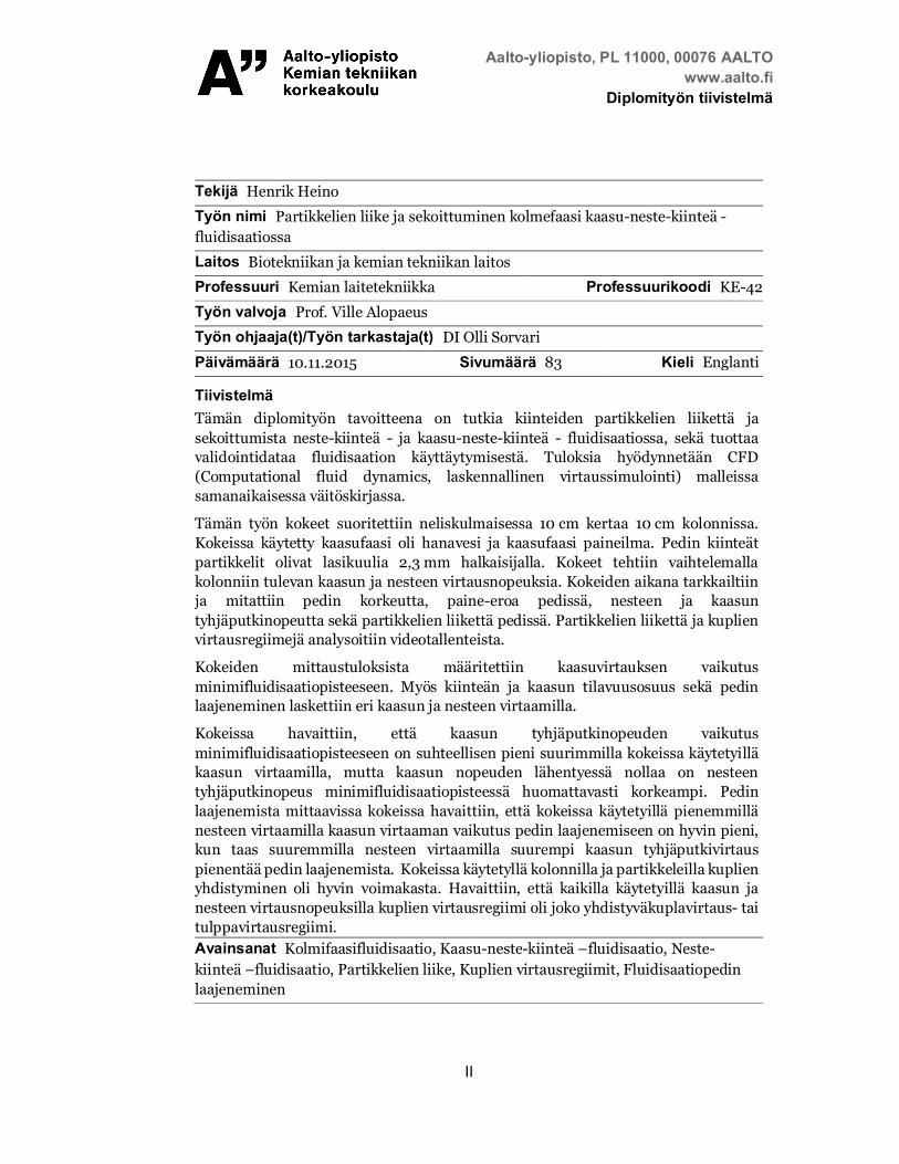
Tekijä Henrik Heino
Työn nimi Partikkelien liike ja sekoittuminen kolmefaasi kaasu-neste-kiinteä -fluidisaatiossa
Laitos Biotekniikan ja kemian tekniikan laitos
Professuuri Kemian laitetekniikka Professuurikoodi KE-42
Työn valvoja Prof. Ville Alopaeus
Työn ohjaaja(t)/Työn tarkastaja(t) DI Olli Sorvari
Päivämäärä 10.11.2015 Sivumäärä 83 Kieli Englanti
TiivistelmäTämän diplomityön tavoitteena on tutkia kiinteiden partikkelien liikettä jasekoittumista neste-kiinteä - ja kaasu-neste-kiinteä - fluidisaatiossa, sekä tuottaavalidointidataa fluidisaation käyttäytymisestä. Tuloksia hyödynnetään CFD(Computational fluid dynamics, laskennallinen virtaussimulointi) malleissasamanaikaisessa väitöskirjassa.
Tämän työn kokeet suoritettiin neliskulmaisessa 10 cm kertaa 10 cm kolonnissa.Kokeissa käytetty kaasufaasi oli hanavesi ja kaasufaasi paineilma. Pedin kiinteätpartikkelit olivat lasikuulia 2,3 mm halkaisijalla. Kokeet tehtiin vaihtelemallakolonniin tulevan kaasun ja nesteen virtausnopeuksia. Kokeiden aikana tarkkailtiinja mitattiin pedin korkeutta, paine-eroa pedissä, nesteen ja kaasuntyhjäputkinopeutta sekä partikkelien liikettä pedissä. Partikkelien liikettä ja kuplienvirtausregiimejä analysoitiin videotallenteista.
Kokeiden mittaustuloksista määritettiin kaasuvirtauksen vaikutusminimifluidisaatiopisteeseen. Myös kiinteän ja kaasun tilavuusosuus sekä pedinlaajeneminen laskettiin eri kaasun ja nesteen virtaamilla.
Kokeissa havaittiin, että kaasun tyhjäputkinopeuden vaikutusminimifluidisaatiopisteeseen on suhteellisen pieni suurimmilla kokeissa käytetyilläkaasun virtaamilla, mutta kaasun nopeuden lähentyessä nollaa on nesteentyhjäputkinopeus minimifluidisaatiopisteessä huomattavasti korkeampi. Pedinlaajenemista mittaavissa kokeissa havaittiin, että kokeissa käytetyillä pienemmillänesteen virtaamilla kaasun virtaaman vaikutus pedin laajenemiseen on hyvin pieni,kun taas suuremmilla nesteen virtaamilla suurempi kaasun tyhjäputkivirtauspienentää pedin laajenemista. Kokeissa käytetyllä kolonnilla ja partikkeleilla kuplienyhdistyminen oli hyvin voimakasta. Havaittiin, että kaikilla käytetyillä kaasun janesteen virtausnopeuksilla kuplien virtausregiimi oli joko yhdistyväkuplavirtaus- taitulppavirtausregiimi.Avainsanat Kolmifaasifluidisaatio, Kaasu-neste-kiinteä –fluidisaatio, Neste-kiinteä –fluidisaatio, Partikkelien liike, Kuplien virtausregiimit, Fluidisaatiopedinlaajeneminen
III
Acknowledgements
I would like to thank my supervisor Professor Ville Alopaeus for offering the Thesis
position and all the guidance during the Thesis. I would also like to thank my
instructor Olli Sorvari letting me work on my own pace and always giving a helping
hand whenever needed. In addition, I would like to thank everybody in the
Chemical Engineering laboratory for all the help they offered me.
I would like to also thank Michelle Lai for help with language troubles and for
proofreading.
Special thanks goes to my brother Juhana and sister Anna-Maria for always
helping me in whatever I asked and to my dad Seppo for guiding, encouraging and
supporting me in everything I have done. Above all, I want to thank my mother Lea
for everything she ever did for me.
Espoo, Finland, 10 November 2015
Henrik Heino
IV
Table of Contents
Literature part ...................................................................................................... 1
1 Introduction ....................................................................................................... 1
2 Fluidization ....................................................................................................... 2
3 Gas-Liquid-Solid fluidization .............................................................................. 4
3.1 Co-current bubble flow regimes .................................................................. 6
3.2 Flow regions in vortical-spiral flow regime .................................................. 9
3.2.1 Descending flow region ...................................................................... 10
3.2.2 Vortical flow region............................................................................. 11
3.2.3 Fast-bubble flow region ...................................................................... 11
3.2.4 Central plume region .......................................................................... 12
3.3 Bubble wake model .................................................................................. 12
3.4 Bubble characteristics .............................................................................. 13
3.5 Particle velocity distributions..................................................................... 15
3.5.1 Channeling ........................................................................................ 17
3.5.2 Gulf-streaming ................................................................................... 18
3.6 Solids flow structure in gas-liquid-solid fluidized bed ................................ 19
3.7 Forces affecting on the particles ............................................................... 20
3.8 Other fluidization characteristics ............................................................... 22
3.8.1 Hold-up .............................................................................................. 22
3.8.2 Pressure drop .................................................................................... 24
3.8.3 Bed expansion ................................................................................... 26
3.9 Other factors affecting on fluidization ........................................................ 26
3.9.1 Distributor .......................................................................................... 27
3.9.2 Particle shape, size and surface properties ........................................ 28
3.10 Particulate and aggregative systems ...................................................... 29
3.10.1 Froude number ................................................................................ 29
3.10.2 Local heterogeneity index ................................................................ 30
3.10.3 Global nonideality index ................................................................... 33
V
3.10.4 Discrimination number ..................................................................... 35
4 Fluidization processes in practice ................................................................... 36
4.1 Gas-liquid-solid fluidization processes ...................................................... 37
4.2 Liquid-solid fluidization processes ............................................................ 38
5 Mixing of solid particles ................................................................................... 38
5.1 Mixing index ............................................................................................. 40
5.2 Mixing time ............................................................................................... 41
6 Particle movement tracking ............................................................................. 41
6.1 Positron emission particle tracking ........................................................... 42
6.2 Radioactive particle tracking ..................................................................... 42
6.3 Imaging techniques .................................................................................. 43
6.4 Particle image velocimetry ........................................................................ 44
6.5 Three-dimensional particle tracking velocimetry ....................................... 45
6.6 Multiple color tracers ................................................................................ 45
6.7 Magnetic particle tracking ......................................................................... 45
6.8 Thermal tracer tracking............................................................................. 46
Experimental part ............................................................................................... 48
7 Experimental setup ......................................................................................... 48
8 Operation principle .......................................................................................... 50
9 Used materials ................................................................................................ 50
9.1 Solid particles ........................................................................................... 50
9.2 Liquid phase ............................................................................................. 55
9.3 Gas phase ................................................................................................ 55
10 Testing equipment installment....................................................................... 55
10.1 Data logging equipment installment ........................................................ 55
10.2 Gas flowmeter installment ...................................................................... 56
10.3 Liquid flow meter installment .................................................................. 56
11 Results.......................................................................................................... 56
VI
11.1 Minimum fluidization ............................................................................... 56
11.2 Hold-ups ................................................................................................. 62
11.2.1 Solids hold-up .................................................................................. 62
11.2.2 Gas hold-up ..................................................................................... 63
11.3 Bed expansion........................................................................................ 66
11.4 Particle movement .................................................................................. 68
11.4.1 Liquid-solid fluidization ..................................................................... 68
11.4.2 Gas-liquid fluidization ....................................................................... 71
12 Recommendations for improvements and future work .................................. 74
12.1 Particles motion detection and tracking .................................................. 74
12.2 Refractive index matching ...................................................................... 75
12.3 Observing all sides of the column ........................................................... 75
12.4 Paint for tracking particles ...................................................................... 75
12.5 Defining the height of the bed ................................................................. 75
12.6 Bubble size measurements .................................................................... 76
12.7 Gas and liquid valves ............................................................................. 76
12.8 Homogenize the liquid and gas flows and reducing the sizes of bubbles
entering the bed ............................................................................................. 77
12.9 Reduce column shaking ......................................................................... 77
13 References ................................................................................................... 79
VII
Nomenclature
′ a factor related to the variables of the solids
area below the voidage-velocity expansion curve [m2]
corresponding area of in real fluidization [m2]
Archimedes number
surface area of sphere [m2]
surface area of a particle [m2]
average concentration of tracer particles in the bed
mean bubble size [m]
particle diameter [m]
friction factor / volume fraction
( ) drag force ratio
gravitational force [N]
drag force [N]
effective drag force [N]
buoyancy [N]
Froude number
acceleration of gravity [m/s2]
conversion factor
height of the fluidized bed [m]
height of the static bed [m]
, effective height of the bed [m]
height of the fixed bed at minimum fluidization conditions [m]
mass [g]
mixing index
number of tracer particles in a sample

VIII
number of tracer particles in the whole bed
number of particles in a sample
Reynolds number
cross-section area of the column [m2]
velocity [m/s]
superficial fluid velocity [m/s]
bubble rising velocity [m/s]
superficial fluid velocity at minimum fluidization conditions [m/s]
∆ pressure drop of the channeling bed [Pa]
∆ pressure drop [Pa]
− static pressure gradient
superficial velocity of fluid [m/s]
weight of the particles in the bed [g]
xd Channeling factor
suspension density [kg/m3]
density of fluid [kg/m3]
density of liquid [kg/m3]
density of a particle [kg/m3]
density of solid [kg/m3]
voidage
overall bed void fraction at minimum fluidization conditions
gas hold-up
liquid hold-up
solid hold-up
sphericity parameter
viscosity [mPas]
1
Literature part
1 Introduction
Fluidization is a process where solid particles are suspended in a continuous liquid
or gas phase. The fluidization process in commonly employer in a wide-range of
industries, such as oil refining and energy production. This thesis focuses on
fluidization processes where liquid forms the continuous phase and gas phase is
non-existent or in a form of bubbles.
The liquid-solid and gas-liquid-solid fluidization technologies have been in use
since the beginning of the 20th century. The earliest industrial gas-liquid-solid
fluidization process was coal hydrogenation taking place in a slurry bubble column.
In coal hydrogenation the pulverized coal reacts with hydrogen forming motor fuels.
Utilization of the process had its prime during World War II in Germany where the
production of mainly aviation fuel peaked at 4.2 million barrels. The production
method was phased out after the war. The first commercial co-current gas-liquid-
solid fluidization reactor was applied in hydrotreating the petroleum resins in 1968.
The process is currently employed, amongst others, in hydrotreating of heavy and
synthetic crude oils, and it is an important part of the oil refining plants.[1]
In a gas-liquid-solid fluidization reactor, which hydrotreats heavy hydrocarbons, the
fluidized solid phase is composed of catalyst particles. The solid catalyst particles
are supported by an upward flow of liquid hydrocarbons and the hydrogen, needed
for hydrogenation, is fed to the bottom of the reactor co-currently with the liquid.[1]
One of the greatest advantages of the fluidized bed reactors compared to fixed bed
reactors is that the fluidized bed reactors do not necessarily need to be stopped
during the change of the catalyst.[1] The solid particles can be simultaneously
removed and replaced while the fluidization is ongoing.
Another advantage of the fluidized beds is the effective mixing inside the catalyst
bed. Consequently, the temperature differences within the bed are usually small.
However, it is possible for stagnant regions to be formed within the bed in which
2
mixing is nonexistent. In case a stagnant region is formed in an exothermic reactor
the temperature begins to rise locally due to accelerating reaction and decreased
heat transfer. The condition is known as hot spot.[1]
The effective and safe exploitation of these advantages of liquid-solid and gas-
liquid-solid fluidization reactors requires knowledge of the particle movement
patterns. More throughout understanding would enable better design of catalyst
replacement systems, lessen the risk of hazardous hot spot formation and possibly
open new ways to safely increase the yield of these reactors.
The goal of this Thesis is to obtain measurement data of the liquid-solid and gas-
liquid-solid fluidized bed behavior, the particle movement and particle mixing in
laboratory scale column. The measurement data is used to validate CFD
(computational fluid dynamics) models as a part of concurrent PhD thesis.
2 Fluidization
Fluidization is a phenomenon in which solid particles are agitated upwards by a
fluid stream in a vertical column. The upward streaming fluid can be either gas or
liquid. Solid particles can be anything from a powder-like substance to metal
particles. Fluidization is done usually in a column with a circular cross-section but
also other shapes.[2-5]
Fluid flows through a permeable distribution plate into the bed of solid particles.
The distribution plate spreads the flow and holds the solid particles in a fixed state,
when the fluid stream velocity is not high enough to fluidize the particles.[3,5]
Normally a column incorporates a homogenization section below the distribution
plate, which function is to homogenize the fluid stream along the cross-section as
evenly as possible.[3] Schematic design of the fluidization column is presented in
Figure 1.
Above the distribution plate there are three distinctive regions: the gas-liquid
distribution region, the bulk fluidized bed region, and the freeboard region. In the
distribution region, the distribution plate gives the bubbles a specific size. The

3
hydrodynamics in the distribution region is strongly dependent on the design of the
distribution plate. The bulk fluidized bed region includes the main part of the
fluidized bed, where the hydrodynamics are dependent on the operation conditions
of fluidization. The freeboard region is located above the bulk fluidized bed region
and containing mainly liquid, rising bubbles and only some entrained particles. With
large and heavy particles the entrainment is less significant than with light and
small particles.[1] Regions in the fluidized bed are also presented in Figure 1.
Homogenizationsection
Distribution plate
Gas-liquiddistribution region
Bulk fluidized bedregion
Freeboardregion
Gas Liquid
Gas
Liquid
Figure 1. Fluidization column.
4
When the fluid starts to flow, the frictional drag between the fluid and the particles
increases so that frictional drag becomes equal to the weight of the particles
subtracted by buoyancy. This causes the particles to rearrange in a way that the
particles generate the least resistance for the fluid flow.[6] At this point the bed is
called expanded bed although the bed is not yet expanding substantially[4,7] and
can even contract depending on the initial state of the bed as observed in the
experiments of this thesis (paragraph 11.1 ). The particle bed structure continues
to rearrange until it reaches the loosest form of packing. When the flow rate is
further increased the particles separate from the structure, are lifted from the
distribution plate, and become supported by the fluid flow i.e. the state of the solid
particles change from fixed to fluidized.[6] The velocity in which this change occurs
is called minimum fluidization velocity.[3]
After the minimum fluidization, the increase in the fluid velocity causes the bed to
expand further. The bed keeps expanding until the fluid velocity is high enough to
convey the particles out of the column. This phenomenon is called hydraulic or
pneumatic transport depending on if the fluid is liquid or gas, respectively.[3]
Fluidization can be gas-solid, liquid-solid or gas-liquid-solid. Generally, the concept
is the same in all fluidization: gas or liquid is fed from the bottom to the bed of solid
particles that causes the particles to lift up from the surface when the velocity is
fast enough. Nevertheless there are still some differences in how the fluidization
behaves amongst different fluids. As an example, in liquid-solid fluidization the
particles are distributed more homogeneously whereas in gas-solid fluidization the
particles tend to have more aggregative behavior.[4]
3 Gas-Liquid-Solid fluidization
In gas-liquid-solid fluidization all the phases, gas, liquid and solid are present. In
this type of fluidization, the solid particles are suspended in the gas or liquid phase.
Gas-liquid-solid fluidization has multiple operating modes. These modes are
defined by which phase is continuous, whether the gas and liquid phases flow
counter-currently or co-currently, and where the phases are fed to the column.[1,8]
5
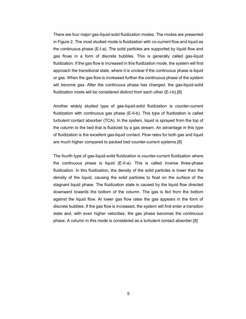
There are four major gas-liquid-solid fluidization modes. The modes are presented
in Figure 2. The most studied mode is fluidization with co-current flow and liquid as
the continuous phase (E-I-a). The solid particles are supported by liquid flow and
gas flows in a form of discrete bubbles. This is generally called gas-liquid
fluidization. If the gas flow is increased in this fluidization mode, the system will first
approach the transitional state, where it is unclear if the continuous phase is liquid
or gas. When the gas flow is increased further the continuous phase of the system
will become gas. After the continuous phase has changed, the gas-liquid-solid
fluidization mode will be considered distinct from each other (E-I-b).[8]
Another widely studied type of gas-liquid-solid fluidization is counter-current
fluidization with continuous gas phase (E-II-b). This type of fluidization is called
turbulent contact absorber (TCA). In the system, liquid is sprayed from the top of
the column to the bed that is fluidized by a gas stream. An advantage in this type
of fluidization is the excellent gas-liquid contact. Flow rates for both gas and liquid
are much higher compared to packed bed counter-current systems.[8]
The fourth type of gas-liquid-solid fluidization is counter-current fluidization where
the continuous phase is liquid (E-II-a). This is called inverse three-phase
fluidization. In this fluidization, the density of the solid particles is lower than the
density of the liquid, causing the solid particles to float on the surface of the
stagnant liquid phase. The fluidization state is caused by the liquid flow directed
downward towards the bottom of the column. The gas is fed from the bottom
against the liquid flow. At lower gas flow rates the gas appears in the form of
discrete bubbles. If the gas flow is increased, the system will first enter a transition
state and, with even higher velocities, the gas phase becomes the continuous
phase. A column in this mode is considered as a turbulent contact absorber.[8]
6
Figure 2. Fluidization operating modes.[8]
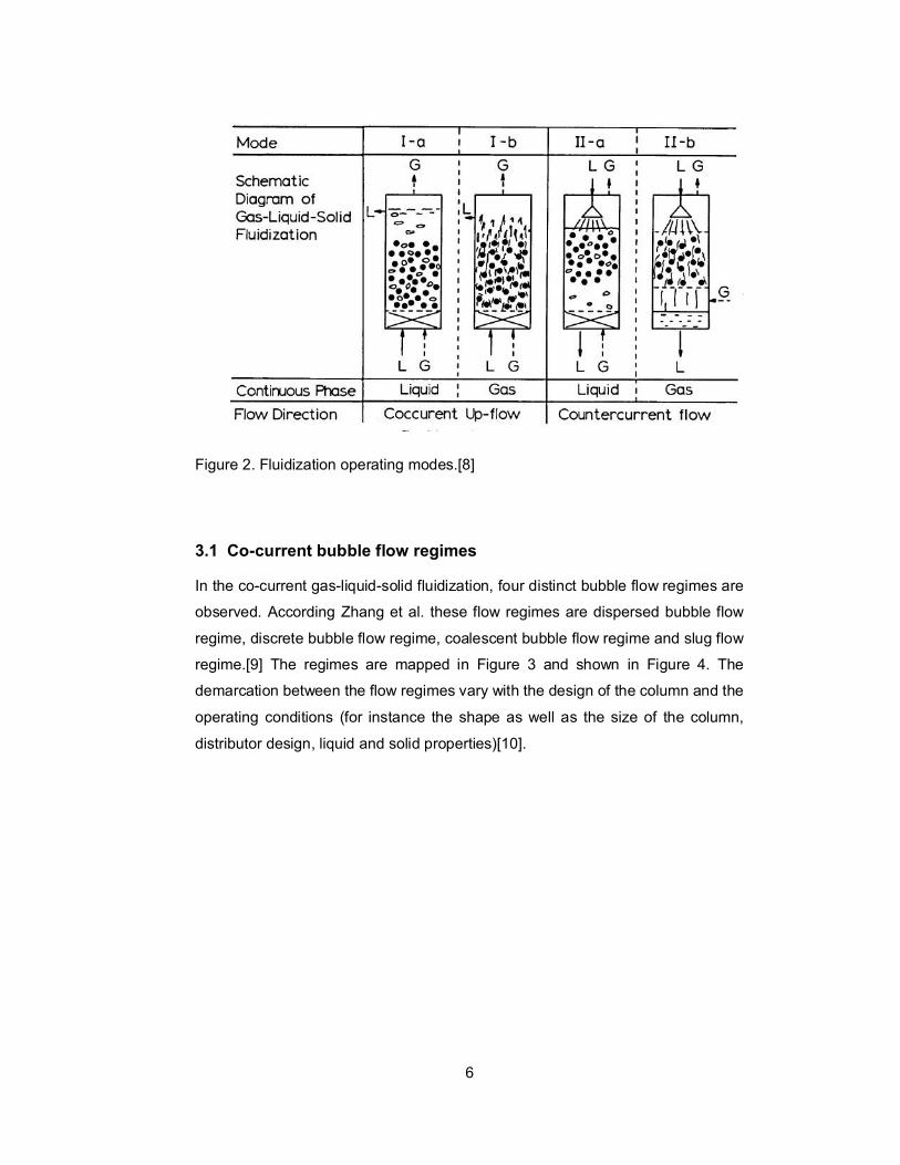
3.1 Co-current bubble flow regimes
In the co-current gas-liquid-solid fluidization, four distinct bubble flow regimes are
observed. According Zhang et al. these flow regimes are dispersed bubble flow
regime, discrete bubble flow regime, coalescent bubble flow regime and slug flow
regime.[9] The regimes are mapped in Figure 3 and shown in Figure 4. The
demarcation between the flow regimes vary with the design of the column and the
operating conditions (for instance the shape as well as the size of the column,
distributor design, liquid and solid properties)[10].
7
Figure 3. Flow regime map.[9]
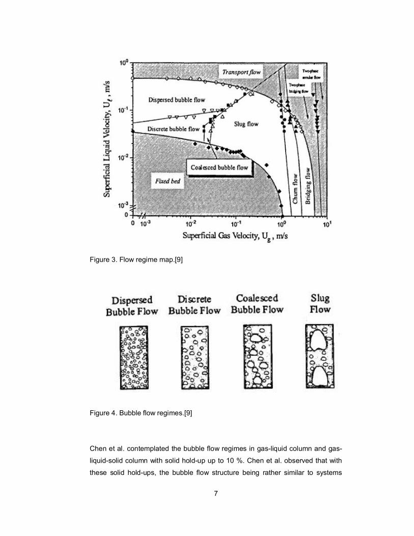
Figure 4. Bubble flow regimes.[9]
Chen et al. contemplated the bubble flow regimes in gas-liquid column and gas-
liquid-solid column with solid hold-up up to 10 %. Chen et al. observed that with
these solid hold-ups, the bubble flow structure being rather similar to systems

8
without solids, only the flow structure sizes were changing. Chen et al. wrote a
study concerning the three different bubble flow regimes: dispersed bubble flow,
vortical-spiral flow and turbulent flow regime. From which the vortical-spiral flow
and turbulent flow regime are also considered as sub-regions of the coalesced
bubble regime.[10]
Discrete bubble flow occurs in the fluidized state with low liquid flow rates. When
the gas flow is introduced, a small amount of small bubbles appear. Bubble size
distribution is narrow and the sizes are strongly depending on the distributor
design. When gas flow is increased enough, the bubbles start to coalesce.[9]
In the dispersed bubble flow regime the bubbles are small and the sizes are rather
uniform in the whole column.[10,11] Bubbles also tend to rise rectilinearly in the
column. The liquid flows downward mostly straight between the rising gas bubble
streams.[10] In the dispersed bubble flow regime the liquid flow velocity is higher
than in the discrete bubble flow. What separates the dispersed flow regime from
discrete flow regime is that the bubble size formation is rather independent of
distributor.[9]
What regimes there are in the system depends strongly on the solid particle sizes
and densities. For example in water-air-glass sphere system the discrete bubble
flow regime does not exist if the particles are small because coalescing of bubbles
starts immediately when the gas flow is introduced. In the systems with larger
particles, more bubble break up is occurring. This indicates that the coalescent
bubble flow regime is emerging in narrower gas and liquid flow velocity interval.[9]
In the vortical-spiral flow regime the superficial gas velocity is higher than in
dispersed bubble flow regime. When the gas velocity is increased from the
velocities used in the dispersed bubble flow regime, the bubbles start to migrate
towards the center of the column in clusters and start the spiral motion. At this
point, the coalescence of the bubbles is not yet significant. When the gas flow is
further increased, the bubbles starts to coalesce and break-up while the clusters
diminish and the spiral motion intensifies.[10]

9
In the turbulent flow regime there are large bubbles separated by a certain distance
from each other. Turbulent flow regime emerges when the bubbles coalesce
intensively and, consequently, interrupts the continuous spiral flow pattern of the
central bubble flow. The momentum of the bubbles wakes are transferred to
surrounding liquid and the liquid mixing is caused mainly by the bubble wakes. The
liquid flow pattern is much more chaotic than in the vortical spiral flow regime. The
mixing in the top and the bottom of the column is not as rapid in turbulent flow
regime as in vortical spiral flow regime.[10]
Slug flow regime is occurs when the gas velocity is increased enough.[9] In the
slug flow regime, the bubbles are even larger[11] and the shape of the bubbles
resemble bullets[9]. The diameter of the bubble can be the same as the diameter
of the column.[11] In addition to these large bubbles, in slug flow regime there are
also many smaller bubbles, which follow the larger ones.[9] Slugging does not
occur in large diameter columns.[1]
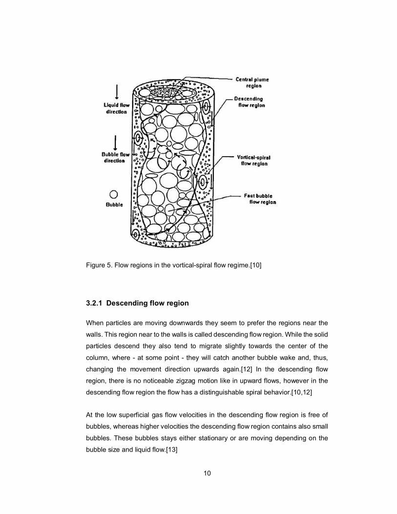
3.2 Flow regions in vortical-spiral flow regime
Larachi et al. identified three different flow regions in gas-liquid-solid fluidization
vortical-spiral flow regime: fast bubble flow region, descending flow region and
vortical flow region.[12] In addition to those Tzeng et al. observed in their study the
central plume region in the center of the column.[10,13] The flow regions are
presented in Figure 5.
It is important to acknowledge that the boundaries between regions are not exact
and peculiar behavior in one region can occur also in other regions.[12]
10
Figure 5. Flow regions in the vortical-spiral flow regime.[10]
3.2.1 Descending flow region
When particles are moving downwards they seem to prefer the regions near the
walls. This region near to the walls is called descending flow region. While the solid
particles descend they also tend to migrate slightly towards the center of the
column, where - at some point - they will catch another bubble wake and, thus,
changing the movement direction upwards again.[12] In the descending flow
region, there is no noticeable zigzag motion like in upward flows, however in the
descending flow region the flow has a distinguishable spiral behavior.[10,12]
At the low superficial gas flow velocities in the descending flow region is free of
bubbles, whereas higher velocities the descending flow region contains also small
bubbles. These bubbles stays either stationary or are moving depending on the
bubble size and liquid flow.[13]
11
3.2.2 Vortical flow region
In the area between the fast-bubble flow region and descending flow region there
is a region called vortical flow region.[10,12] In this region the particles have just
exited the fast-bubble flow and have not yet moved into the descending flow. The
particles normally stay in the vortical flow region less than a second and the
movement of the particles are very rapid and intense. It is very difficult to mark
boundaries, especially where the vortical flow region ends and where the
descending flow region begins, because of the dynamic nature of the flows.[12] So
the entire region moves back and forth according the neighboring fast bubble flow
region.[10]
The vortices usually form near the free bed surface and, from there, tend to move
downwards until at some point they disappear. When the superficial gas velocity is
increased the vortices become more unstable. The size of the vortex depends
strongly on the superficial gas velocities, the size increases with the gas flow
velocity until the point of bubbly-churn turbulent transient velocity, after which the
size stays rather constant.[13] The mixing of the phases is extensive in this
region.[10]
3.2.3 Fast-bubble flow region
The remarkable bubble coalescence and break-up is occurring in the fast bubble
flow region. The bubble break up is caused partly by local flow turbulences. The
bubbles are moving in a wavelike motion in a two-dimensional column where one
dimension was considerably smaller than other dimensions. When experiments
were done in three-dimensional column the bubbles moved in a spiral like motion.
Bubbles tend to move in clusters at lower superficial gas flow velocities or as
coalesced bubbles in higher superficial gas flow velocities.[10,13] The behavior of
fast bubble flow region dictates the macro hydrodynamics of the flow system in
vertical-spiral flow regime.[10]
According to Chen et al., when increasing the superficial gas velocity, the width of
the fast-bubble region increases linearly until a certain point where the width
remains constant. The maximum width of the fast bubble flow region is of the same
order as the large coalescent bubbles in the turbulent flow regime. Increasing the
12
superficial gas velocity also increases the pitch of the spiral motion to the point
where the pitch starts to decrease with the further increase in the gas velocity.[10]
Respectively, the increase in superficial liquid velocity slows down the bubble
coalescence and decreases the width of the fast bubble flow region. Increase in
superficial liquid flow velocity also decreases the spiral pitch. In addition, the
increase of the liquid velocity decreases the sizes of the bubbles.[10]
3.2.4 Central plume region
Tzeng et al. observed that the central plume region exists in the center of the
column core as well. This central plume region is surrounded by the fast bubble
flow region. In the central plume region, the bubble sizes are more uniform
compared to bubbles in the fast bubble flow region. To add, in the fast bubble flow
region, the bubbles interact more intensively with each other than in central plume
region, therefore the bubble coalescence and break-up is more common in the fast
bubble flow region than in central plume region. In high superficial gas velocities,
the coalescence still occurs, however more in the vertical direction, rather than
lateral as in fast-bubble flow region.[10,13]
3.3 Bubble wake model
The wake phenomena plays a significant role in the understanding the bed
hydrodynamics in gas-liquid-solid fluidized bed. The wake phenomena is
responsible for a large part of the particle movement in the vertical direction and,
thus, induces mixing in the fluidized bed considerably. There are two regions of the
wake that moves the particles: a stable solid region, where the particles are moved
upwards following the leading bubble, and shedding wake region, where the solids
are pushed towards the liquid-solid emulsion. The shedding region is able to collect
particles from the stable region, so that the particles will not reach the surface of
the bed every occasion. Vice versa, the particles can move to the stable solid
region, where the particles are transferred towards the surface of the bed. After the
particles are shed from the wake they start to move downwards.[12]
By forming a distribution for the axial location where the particle is shed from the
wake, it can be seen that the wake shedding tends to be more intensive when
13
moving further away from distribution plate. Half of the shedding occurs in the
upper third of the bed. For wake phenomena, it is also peculiar that the bubble and,
thus, the wake velocity varies during the rise as well. This is due to the bubbles
interactions with other bubbles such as bubble coalescence and bubble break-
ups.[12] In addition, when the bubble is accelerating while ascending, the wake
grows in size and collects more particles.[1]
It is possible to contour the distinct areas in the cross-section, where the bubble
wakes are active. In these areas, the particle movement upward is also significant.
The particles near the distribution plate, when caught by the wake, first moves
towards the center of the column while traveling up.[12] The wake shedding
phenomena is strongly connected to the flow path the bubble takes. For example,
the interaction with vortices causes particles to shed from alternating sides, which
again causes the bubble to move in zigzag motion.[1] Interaction with other
bubbles can also cause zigzag motion.[12]
To conclude, the bubble wake is significant factor when assessing phenomena in
the fluidized bed such as solids mixing, particle entrainment into the freeboard, and
bed contraction when introducing the first bubbles in the system.[1] When a bubble
is rising upwards in gas-liquid-solid fluidized bed, the bubble is followed by a liquid
having a flow velocity higher than the average liquid velocity in the column.
Consequently, the liquid following the bubbles have shorter residence time than
the water not following the bubbles. This causes the bed to contract until the point
of critical gas flow, after which the bed starts to expand.[14]
3.4 Bubble characteristics
The performance of the fluidization is strongly determined by the behavior of the
bubbles in the gas-liquid-solid fluidization. Knowledge of the hydrodynamic
properties including bubble size, bubble rise velocity, velocity distribution and
bubble distribution is an important part in understanding the behavior of the gas-
fluid-solid fluidized bed. This is, because they define in some extent the
hydrodynamic properties like liquid flow patterns, solids mixing and gas-liquid
interfacial area.[15]
14
Sizes of the holes in the distribution plate is a significant factor when defining the
initial size of the bubbles created. Large holes produces larger bubbles, which
leads to greater heterogeneity in the bed and the small holes generates smaller
bubbles, which smaller bubbles has tendency to merge into larger bubbles while
moving upwards losing the benefit for the smaller holes if the bed is high.[16] Other
factors defining the initial bubble size are buoyancy, viscous drag, surface tension
and inertia. Bubble collision with single particles in the bed also induce breaking
up the bubbles, if the particle diameter is larger than the diameter of the bubble. If
bubble is penetrated with multiple particles- as usually is in fluidized bed- it induces
bubble instability and, thus, also bubble breakage.[1]
The increase in liquid flow velocity decreases the bubble size until a certain point
in which the increase of the liquid flow velocity is no more effective.[1] In the
dispersed flow regime, the bubble size reaches minimum near the minimum
fluidization velocities. When the liquid velocity is increased from that the bubble
size becomes larger.[17]
The bed expansion parameter Hf/H0 is the ratio between fluidized bed height and
static bed height. It is related to solid hold-up and to the mean bubble size in the
bed. In the dispersed bubble flow regime, the mean bubble size varies only slightly
when bed expansion parameter increases. On the other hand, in the coalescent
bubble flow regime the mean bubble size increases substantially when the bed
expansion parameter increases. In the slug flow regime, the bubble size increases
moderately with the increase in bed expansion parameter.[15]
The increase in bubble size above the distributor is due to the bubble coalescence.
The bubble coalescence is more intense in the bed of small particles.[1] In gas-
liquid-solid fluidization the bubble size distribution varies substantially with the axial
location and with flow regime. According Matsuura and Fan, the effect the particle
size has on the bubble size and bubble size distribution is rather small. However,
the flow regime has a great effect on the mean bubble size.[15]
In the gas-liquid-solid fluidized bed, the bubble rising velocities depends strongly
on the size of the bubble and, therefore, also on the flow regime.[1] In the slug flow
regime, the bubble rising velocity can be estimated with equation 1. It is also
15
noticeable that the bubble rising velocities behind the slugs are higher than similar
bubbles in dispersed bubble flow regime.[15]
= 3.4 1
Where dn is the mean bubble size.
The distributions of the bubble rise velocities are rather similar in coalesced bubble
flow regime and in dispersed bubble flow regime. The small difference between
velocity distribution curves with the dispersed flow regime and coalescent flow
regime demonstrated that the coalescent flow regime the bubble velocity is slightly
faster in the coalescent flow regime and the velocities are more narrowly distributed
in the dispersed flow regime.[15]
3.5 Particle velocity distributions
In the fast-bubble flow region and in the descending flow region, the particle
movement has a longer amplitude than in the vortical flow region. These two
regimes comprises the gulf-streaming (gross circulation) in the bed.[12]
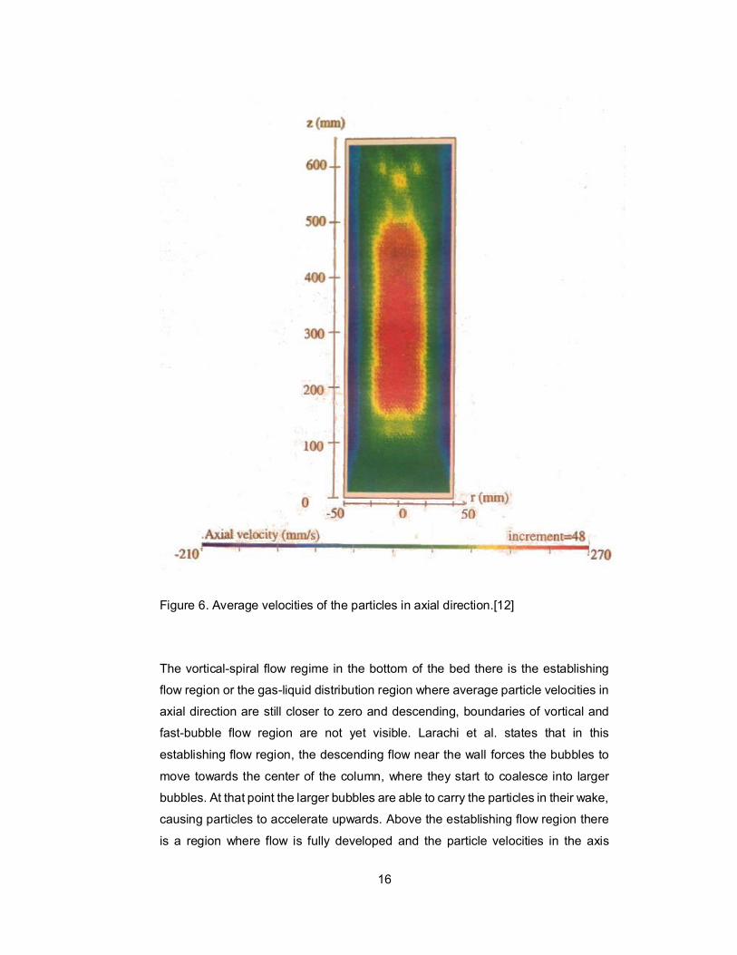
Larachi et al. drew a Figure 6 of average velocities of the particles in axial direction
highlighted by different colors. The figure clearly shows the velocity vector
distribution. Whereas in the middle of the column the rapidly upward moving
particles comprises the fast-bubble flow region, the descending particle velocities
are greatest in the descending flow regions. Between these regions there is a
distinguishable flow inversion region, the vortical flow region, where the particle
velocities in the axial direction are close to zero.[12]
16
Figure 6. Average velocities of the particles in axial direction.[12]
The vortical-spiral flow regime in the bottom of the bed there is the establishing
flow region or the gas-liquid distribution region where average particle velocities in
axial direction are still closer to zero and descending, boundaries of vortical and
fast-bubble flow region are not yet visible. Larachi et al. states that in this
establishing flow region, the descending flow near the wall forces the bubbles to
move towards the center of the column, where they start to coalesce into larger
bubbles. At that point the larger bubbles are able to carry the particles in their wake,
causing particles to accelerate upwards. Above the establishing flow region there
is a region where flow is fully developed and the particle velocities in the axis

17
direction is relatively stable. Above the fully developed region there is a region
called disengagement part. The disengagement part is where the axial particle
velocities decelerates from the velocities in the middle and particles changes
direction and start flowing downwards.[12]
Larachi et al. measured the turbulence in two directions: axial and radial. Intensive
turbulence in the radial direction occurs in the fast-bubble flow region where the
particles are swinging and rocking back and forth. The most intensive turbulence
in radial direction is the decelerating zone where the wakes discharge the rising
particles and the particles change in flow direction. In the axial direction, the
turbulence is the most intensive in the vortical flow region between the fast-bubble
flow region and descending flow region.[12]
3.5.1 Channeling
Channeling is a phenomenon where the fluid and
particle flow velocities are not distributed evenly in
the cross-section of the column. In fluidization the
channeling occurs when a great portion of the fluid
passes through the fluidized bed within a small
cross-sectional area and only a small portion of
the fluid passes through the bed evenly.[16,18]
Channeling fluidized bed is illustrated in Figure 7.
The uneven velocity distribution is a significant
factor when characterizing the hydrodynamics
and mixing characteristics of the fluidized bed[13].
Initially, channeling occurs due to the uneven
pressure profile in the distribution plate.
Consequently, when maldistribution occurs it
establishes the path of least resistance for the fluid
creating a channel where the fluid has greater flow
velocity than the rest of the bed.[16,18]
Figure 7. Channeling and gulf-streaming of fluidized bed.

18
Channeling is a strongly unwanted situation because the contact of the fluid with
the solid particles decreases substantially. Channeling can also cause hotspots
where exothermic reactions take place more than the rest of the bed.[16]
Channeling may also cause termination of fluidization when the pressure drop
decreases leading to the fluid velocity to drop below supporting levels for the
particles in the other parts of the bed.[18]
Courderc and Angelino (1970) cited by Davidson et al. (page 7) states that
channeling can be avoided by using a greater homogenization section and more
efficient fluid distributor.[3] Zenz et al. wrote that channeling can be restrained by
using a distributor plate that has a pressure drop of at least 40% through the
fluidized bed.[16]
In equation 2, a channeling factor xd is shown, which can be expressed by the
difference between expected fluidized bed pressure drop that can be calculated
with the equation 18 and pressure drop of channeled bed and the difference
divided by the pressure drop of expected fluidized bed. Channeling factor can be
used to compare the channeling behavior of different beds. The larger channeling
factor implies greater channeling tendency.[18]
=∆ − ∆
∆2
3.5.2 Gulf-streaming
When the fluidized bed is channeling, it causes phenomena called gulf streaming.
In gulf streaming there is a distinct gross circulation flow pattern where the particles
rise in one part of the column cross-section and in the other part- typically near the
column walls- they are flowing downwards.[7,10,13,19,20] Near the top and the
bottom of the fluidized bed these particle flows combine forming a circular flow
pattern. In gulf streaming, the solid particles are conveyed more rapidly than in
fluidization without channeling and gulf streaming.[3] Gulf streaming has been
observed in both dispersed bubble and coalesced bubble regimes.[10]

19
The existence of the gross circulation flow pattern depends strongly on the
superficial gas velocity.[10] At low superficial gas flow velocities the gulf-streaming
cannot be clearly observed. In these velocities bubbles rise rectilinearly in the
column. If the gas velocity is increased there is a point called critical gas velocity,
where the bubbles near the walls of the column start to shift towards the center
breaking the rectilinear pattern.[13] Gulf streaming can be a more important
mechanism for mixing than the mixing caused by bubbles.[20]
3.6 Solids flow structure in gas-liquid-solid fluidized bed
Cassanello et al. formed a model that can be seen as a simplified structural wake
model. The gas-liquid-solid fluidized bed is divided into three separate “phases” in
order to study the hydrodynamics of the solid particles. These phases are bubble
phase, wake phase and emulsion phase. Where the bubble phase is gas bubbles,
free from solids and liquids, traveling upwards in the column. The wake phase
consists of liquid and solids following bubbles moving upwards. The emulsion
phase consists of liquid and solids traveling downwards in the column.[21]
In the model described by Cassanello et al., there were some generalizations. The
movement of solids is only considered to be due to primary wakes and other
mechanisms are neglected. Another assumption is that the wake is considered to
be moving with the same velocity as the bubble. The third assumption is that there
is continuous mass transfer of particles between the emulsion phase and the wake
phase.[21]
Cassanello et al. found out that in the heterogeneous flow regime velocities of the
solid particles accelerates near the bottom of the column. Afterwards, the velocities
remained constant until they reach the disengagement zone in the upper parts of
the bed, where the velocities decelerate.[21]
Cassanello et al. have also studied the chaotic behavior of the gas-liquid-solid
fluidized bed. In their experiments, the Kolmogorov entropy, describing the
required accuracy of the initial conditions in order to predict the system evolution
was positive in both liquid-solid and gas-liquid-solid fluidization. This suggests that
the fluidized bed was chaotic. The degree of chaoticity increases with increasing
the superficial gas velocity.[22]
20
3.7 Forces affecting on the particles
There are three forces acting on the particles during the fluidization: gravitational
force, buoyancy and drag forces. According the Newton’s first law, when these
forces are balanced, the particles are moving at constant velocity as shown in
equation 3. From these the gravitational force is the only unambiguous force.[23]
+ = 3
There are two ways by which buoyancy force in a fluidized bed is represented in
the literature. One is called apparent buoyancy, and the other Archimedes
buoyancy, and respectively, where is the suspension density and
is the density of the percolating fluid. Because the gravitational force is undisputed,
the buoyancy dispute affects also the magnitude of drag force because the sum of
forces are zero, if the particle is not accelerating.[24]
In laminar flow the Drag force affecting a single particle can be calculated with
Stokes law shown in equation 4.[25]
=3 4
Where µ is viscosity of fluid, V superficial velocity of fluid, dp diameter of the sphere
particle and gc is conversion factor. To cover all the flow conditions with Reynolds
number from 0.001 to 1000 equation 5 was formed.[25]
21
= (3 + 0.45 . )5
In the multiparticle system, the drag force acting on each particle is depending on
the voidage of the system. In order to assess drag force of the bed Fk, the drag
force ratio f(ε) needs to be defined. It is the ratio between the drag force of the bed
and a single particle, as shown in equation 6.[25]
( ) = 6
The voidage indicates the “open” area of the columns cross-section that the solid
particles are not filling. Voidage of the bed can be calculated with equation 7.[26]
= 1 − = + 7
Wen and Yu found out that this relation can be presented as in equation 8.[25]
= . 8
Now the drag force of multi particle system equation 9 can be written.[25]

22
= . (3 + 0.45 . )9
3.8 Other fluidization characteristics
When the bed is fluidized it has distinctive characteristics like hold-ups and
pressure drop. When the fluid is flowing through the bed it is causes a pressure
drop in the fluid. In the other hand, the hold-ups are proportional to the phases
presented in the bed. Phase hold-ups and pressure drops of the bed are strongly
related[1].
3.8.1 Hold-up
In fluidized bed the solid hold-up can be calculated with equation 10.[1,8]
= 10
Where W is weight of the solid particles in the bed, ρs is density of the solid, S is
cross-section area of the column and H is effective height of the bed.[8] The bed
height can typically be measured by visual observation, especially with larger and
heavier particles.[1]
The sum of the gas, solid and liquid hold-ups is one, which is presented in the
equation 11.[1,8]
+ + = 1 11

23
In the steady-state, the static pressure gradient can be presented with equation
12.[1,8]
− = ( + + )12
In equation 12, the frictional drag on the column walls is neglected as well as gas
and liquid acceleration terms.[1] The gas term is usually insignificant compared to
other terms, so it is usually ignored, thus giving the equation 13.[1,8]
− = ( + )13
The solid hold-up can be calculated directly from equation 10; the liquid hold-up
can then be calculated from equation 13, provided that the static pressure gradient
is measured simultaneously.[8] Liquid hold-up can also be evaluated with an
electrical conductivity method.[1] Liquid hold-up can be estimated with
dimensionless correlations rather accurately.[27]
For the gas hold-up it is challenging to develop any correlation that covers all the
circumstances since the gas hold-up is strongly dependent on the flow regime.[1]
Although Larachi et al. later wrote that gas hold-up is affected mainly by solid and
gas inertial forces, it decreases when the liquid capillary and viscous forces are
increased.[27]
Gas hold-up is possible to calculate by combining the equations 11 and 12 to the
equation 14.
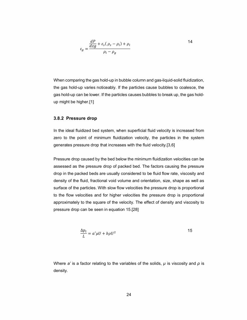
24
=+ ( − ) +
−
14
When comparing the gas hold-up in bubble column and gas-liquid-solid fluidization,
the gas hold-up varies noticeably. If the particles cause bubbles to coalesce, the
gas hold-up can be lower. If the particles causes bubbles to break up, the gas hold-
up might be higher.[1]
3.8.2 Pressure drop
In the ideal fluidized bed system, when superficial fluid velocity is increased from
zero to the point of minimum fluidization velocity, the particles in the system
generates pressure drop that increases with the fluid velocity.[3,6]
Pressure drop caused by the bed below the minimum fluidization velocities can be
assessed as the pressure drop of packed bed. The factors causing the pressure
drop in the packed beds are usually considered to be fluid flow rate, viscosity and
density of the fluid, fractional void volume and orientation, size, shape as well as
surface of the particles. With slow flow velocities the pressure drop is proportional
to the flow velocities and for higher velocities the pressure drop is proportional
approximately to the square of the velocity. The effect of density and viscosity to
pressure drop can be seen in equation 15.[28]
∆= +
15
Where a’ is a factor relating to the variables of the solids, µ is viscosity and ρ is
density.
25
When the pressure drop generated by the bed is enough to support the particles
throughout the bed, the bed is in fluidization, so that the particles are not supported
by the distribution plate anymore.[5] While increasing the fluid flow velocity further
the pressure drop will stay relatively constant, i.e. the increase in the fluid velocity
will not have a significant difference in the pressure drop of the bed.[3,4]
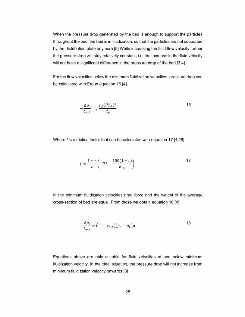
For the flow velocities below the minimum fluidization velocities, pressure drop can
be calculated with Ergun equation 16.[4]
−∆
=( ) 16
Where f is a friction factor that can be calculated with equation 17.[4,28]
=1 −
1.75 +150(1− ) 17
In the minimum fluidization velocities drag force and the weight of the average
cross-section of bed are equal. From those we obtain equation 18.[4]
−∆
= 1 − − 18
Equations above are only suitable for fluid velocities at and below minimum
fluidization velocity. In the ideal situation, the pressure drop will not increase from
minimum fluidization velocity onwards.[3]
26
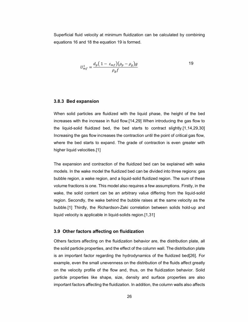
Superficial fluid velocity at minimum fluidization can be calculated by combining
equations 16 and 18 the equation 19 is formed.
=1 − − 19
3.8.3 Bed expansion
When solid particles are fluidized with the liquid phase, the height of the bed
increases with the increase in fluid flow.[14,29] When introducing the gas flow to
the liquid-solid fluidized bed, the bed starts to contract slightly.[1,14,29,30]
Increasing the gas flow increases the contraction until the point of critical gas flow,
where the bed starts to expand. The grade of contraction is even greater with
higher liquid velocities.[1]
The expansion and contraction of the fluidized bed can be explained with wake
models. In the wake model the fluidized bed can be divided into three regions: gas
bubble region, a wake region, and a liquid-solid fluidized region. The sum of these
volume fractions is one. This model also requires a few assumptions. Firstly, in the
wake, the solid content can be an arbitrary value differing from the liquid-solid
region. Secondly, the wake behind the bubble raises at the same velocity as the
bubble.[1] Thirdly, the Richardson-Zaki correlation between solids hold-up and
liquid velocity is applicable in liquid-solids region.[1,31]
3.9 Other factors affecting on fluidization
Others factors affecting on the fluidization behavior are, the distribution plate, all
the solid particle properties, and the effect of the column wall. The distribution plate
is an important factor regarding the hydrodynamics of the fluidized bed[26]. For
example, even the small unevenness on the distribution of the fluids affect greatly
on the velocity profile of the flow and, thus, on the fluidization behavior. Solid
particle properties like shape, size, density and surface properties are also
important factors affecting the fluidization. In addition, the column walls also affects
27
to the fluidization, however the effect is normally considered diminishingly small,
so it is usually ignored[32]. Effect of distributor and particle properties are covered
more closely.
3.9.1 Distributor
The distribution plate’s task is to prevent solids from dropping out of the fluidized
bed and to distribute the fluid flow evenly across the bed.[7,33] The distribution
plate generates a pressure difference for the flowing fluid and generally the greater
pressure difference the distribution plate generates, the more uniform flow it
generates above the plate. However, the greater pressure drop will also causes
the pumping of the fluid o be more expensive. Optimally the pressure drop would
be just enough to ensure the uniform flow velocity distribution.[7]
The fluid flow resistance in the fluidized bed does not change substantially with
increase in fluid flow. However, in the distribution plate, the resistance increases
with the increase in the fluid flow. Indicating that the increase in pressure drop in
the distribution plate has an effect on the fluidization characteristics.[26]
The pressure drop caused by the distribution plate is usually compared with the
pressure drop caused by the bed. There are multiple different recommended ratios
for the ratio between the pressure drop caused by the distribution plate and the
pressure drop caused by the bed.[7,26] In literature, distribution plates can
generate pressure drop ratios normally varying from 0.015 to 0.4 but even higher
ratios can also be used. The distribution plates has been categorized in low
pressure drop and high pressure drop classes. If the pressure drop ratio is between
0.015 and 0.2 it is considered to be a low pressure drop plate; if the pressure drop
ratio is more than 0.4, it is considered as a high pressure drop distribution plate.[26]
The required pressure drop ratio for uniform fluidization depends moderately on
the solid particle size. Siegel wrote that particles with roughly a diameter of 0.5 mm
would require pressure drop ratios greater than 0.25, whereas particles with
diameter of 23 µm would only need approximately 0.15 pressure drop ratio.[34]
The needed pressure drop ratio for uniform fluidization also depends on the fluid
superficial flow velocity. Shi and Fan wrote that if the fluid superficial flow velocity

28
is 1.5 times the minimum fluidization velocity, the pressure drop ratio should be
0.11 with perforated distributor and 0.18 with porous distributor. While the fluid
velocity increases, the needed pressure drop ratio increases also.[33]
3.9.2 Particle shape, size and surface properties
The most important properties of the particles are size, density and flowability. [20]
In addition, roughness and voidage associated with particles should also be
considered.[26]
Defining the size of the particle is rather straightforward with spherical particles.
Only the diameter of the spherical particle is required for defining the size. For other
particles the size can be defined by measuring the volume of the particle and then
defining the diameter of the equivalent volume sphere. There is a parameter called
sphericity Φs shown in equation 20.[7]
=20
Where the sphere and particle are the same volume and the Asph is the surface
area of the equivalent sphere and Apart is surface are of the particle.
The solid particles in the system are usually considered spherical when assessing
the behavior of the particles. Frequently this is not the case, however it is still
important to know how the properties of the particles change with different shapes.
For assessing non-spherical particle properties, there are multiple
correlations.[1,3]
Roughness of the particles adds friction between the particles causing the increase
in bed porosity. In consequence, the pressure drop of the bed will be higher with
rough particles compared to bed with smooth particles. The roughness of the
particle can be assessed by measuring the friction factor of the particles.[26]
29
3.10 Particulate and aggregative systems
In the fluidized bed, there are two states concerning how the particles are
distributed during fluidization. These states are called particulate and aggregative.
In the particulate system, the fluidized particles are distributed uniformly. In
aggregative systems particles are distributed unevenly, which indicates that in
some parts of the fluidized bed the particles are distributed more densely, and in
other parts sparser. Particulate systems are usually associated with liquid-solid
fluidization, whereas aggregative systems are associated with gas-solid
fluidization.[3]
However, the distinction between particulate and aggregative system is not that
simple. In addition to liquid-solid fluidization, the particulate behavior can be
observed also with gas-solid system, when the solid particles are light.[3]
Aggregate behavior can be observed additionally with water and very dense
particles[35], such as copper and lead particles[2,35]. There are not yet any definite
criteria is that applicable under all conditions for defining if the fluidization will
behave as particulate or aggregate system.[35,36]
There are a few methods that helps in distinguishing if the fluidization is
aggregative or particulate. The Froude number explains the quality of the
fluidization.[2,17] The local heterogeneity index describes the local characteristics
of the intermediate states and the global nonideality index describes the bed
expansion characteristics. The discrimination number describes the transition
between particulate and aggregative fluidization.[37]
3.10.1 Froude number
Wilhelm and Kwauk wrote that Froude number provides a suggestive figure that
tells if the fluidization in minimum fluidization is particulate or aggregative. The
equation for Froude number is presented in equation 21. If the Froude number is
less than 0.13, fluidization is particulate; if the number is more than 1.3, the
fluidization is aggregative.[2]
30
= 21
3.10.2 Local heterogeneity index
Local heterogeneity index δ is a relative measure that describes the local
characteristics of the system voidages.[37] This method is valid only in two-phase
fluidization. The index varies between 0 and 1, where 0 is fully homogenous
fluidization and 1 is the most heterogeneous fluidization i.e. slugging[37].
The samples of the fluctuating voidage signal obtained by optical fiber probe is
required for first calculating the standard deviation of voidages. The standard
deviation can be calculated with equation 22.[36,37]
=1
( − )
22
Where n is the number of samples measured with the probe. As a result different
σ values describes the different configurations of phase mixtures. Taking into
account the slugging as the most heterogeneous pattern and that the signal
detected by the probes varies between εmf and 1. Where εmf illustrates the voidage
in dense phase at minimum fluidization and 1 the bubble phase. Thus, with
samples n1 and n2, equations 23, 24 and 25 are obtained.[37]
= + 23
31
= ( = 1 → ) 24
= 1( = 1 → ) 25
Then by combining the equations 22, 23, 24 and 25 we get equation 26 for
standard deviation for slugging, and by deriving that we get equation 27.[37]
=1
− + (1 − )
26
=1
− + (1 − )27
For slugging, the volume fraction of dense phase is f, so we obtain equations 28
and 29.[37]
= 28
1 − = 29
In continuation, by combining equations 27, 28 and 29 we get equation 30.[37]
32
= − + (1− )(1 − )30
From that, when the definition of average voidage is expressed in equation 31, we
acquire the equation 32 from equations 30 and 31.[37]
= + (1 − ) 31
= (1 − ) 1 − 32
The maximum standard deviation can be found by differentiating the equation 32
with respect to f and then setting the derivative to 0.[37]
=1 − 2
2 (1 − )1 − = 0
33
Which derives f=1/2 and by substituting it to equation 32, equation 34 is formed.[37]
33
=1 −
234
And then for any voidage sample with standard deviation, the heterogeneity index
can be defined as in equation 35.[37]
( ) = =2
1 −35
Because the standard deviation changes with velocity U, the heterogeneity index
can also be obtained by integrating between minimum fluidization velocity and
maximum velocity, thus, creating the velocity-averaged heterogeneity index
presented in equation 36.[37]
( ) =∫
−
36
For liquid-solid fluidization, the heterogeneity index number is relatively low and
remains rather constant at all flow velocities[37], which states that liquid-solid
fluidization is usually relatively homogenous and particulate in nature.
3.10.3 Global nonideality index
Global nonideality index fh describes the difference between real and ideal
expansion of the bed. In the ideal expansion there is a linear relationship among
the logarithmic voidage and logarithmic superficial fluid flow velocity. In the ideal
34
case, the area AP below the voidage-velocity expansion curve can be calculated
with equation 37.[36,37]
=37
When U=Utεn we get the equation 38.[36]
= ( )38
And when integrating equation 38 we acquire equation 39.[36]
=+ 1
(1 − ) 39
For any real fluidized beds, the corresponding area is calculated with equation
40.[36]
= 40
AP is generally greater than AR indicating that the real expansion is usually less
than in ideal cases. The global nonideality index fh is calculated with equation 41
35
and it illustrates the difference in the area of the real situation and the ideal
situation. Equation 41 is also represents the differential area under the voidage-
velocity curves. Nonideality index is equal to 0 when the bed is expanding ideally.
When nonideality index is greater than 0 which indicates that the bed is nonideal.
The greater the nonideality index is, the more nonideal the bed expansion is.[36]
=+
= 1 − = 1 −( + 1)∫
(1 − )
41
3.10.4 Discrimination number
When defining the fluidization pattern, the most important factors are particle size,
particle density, fluid density, and fluid viscosity. Dimensionless discrimination
number Dn combines all of these properties. The lower the discrimination number
is, the more uniform the fluidization will be.[37]
= − 42
Where the first bracketed equation represents the effect of particle size and the
fluid viscosity and effect of densities are represented in the second. Re is Reynolds
number and Ar is Archimedes number, which can be calculated with equations 43
and 44, respectively.
= 43
36
=( − )
44
According to Wen and Yu a correlation between Reynolds number as a function of
Archimedes number can be represented as equation 45. A ratio for Archimedes
number and Reynolds number can be obtained through equation 46.[38]
= 33.7 + 0.0408 − 33.7 45
= 1652.0 + 24.546
Liu et al. stated that the local heterogeneity index, global nonideality index and
discrimination number change with similar trends. For particulate fluidization the
discrimination number is between 0 and 104, the global nonideality index is less
than 0.2, and the local heterogeneity index is less than 0.1. On the contrary, for
aggregative fluidization the discrimination number is more than 106, global
nonideality index is more than 0.6, and the local heterogeneity index is more than
0.5. For everything in between, the fluidization is at a transitional state.[37]
4 Fluidization processes in practice
Gas-liquid-solid and liquid-solid fluidization processes has been and are still vastly
used in industries such as chemical, petroleum, environmental, metallurgical and
energy industries.[3] A few of these processes are described more throughout in
following chapters.
37
4.1 Gas-liquid-solid fluidization processes
In gas-liquid-solid fluidization the different phases can be reactants, catalysts,
products or inert. In the same system all the phases can be, for example, reactants
or products like in coal liquefaction. Alternatively, in the same system, the gas and
liquid phases can be reactants and products when the solid is catalyst as in
hydrogenation. If there is an inert phase it can also be in any of the phases. Three
phase fluidization is used also in systems without reactions as in air
humidification.[1]
In addition to hydrotreating, the gas-liquid-solid fluidization is used for example in
bioreactors, wastewater treatment, flue gas treatment, and in other systems.[1]
One of the most important application of the gas-liquid-solid fluidized bed is
hydrotreating in the petroleum industry. The feedstock can be for example heavy
oil, petroleum resin or synthetic crudes from coal and tar sands. Reactions in the
hydrotreating processes are for example cracking, hydrocracking,
hydrodesulfurization, hydrodeoxygenation, hydrodenitrogenation, and
hydrodemetallization. Feedstock is fed to the reactor in liquid phase. In the gas
phase there is hydrogen and the solids are catalysts. In the reactor the temperature
is usually from 300 to 425 °C and the pressure is from 5.5 to 21 MPa.[1]
In bioreactors, the solid phase in fluidization is usually composed of immobilized
cells. The solid particles are made by attaching cells to particles, so that they will
grow into biofilm to the surface of the particles. In the bioreactors the liquid input is
usually so minor that the particles are fluidized with gas flow. The composition of
the gas phase depends on whether the reaction is aerobic or anaerobic. For
aerobic reactions, the gas flow is usually air or oxygen. Whereas in anaerobic
reactions the gas phase used is inert such as nitrogen. These kind of processes
are used for example in production of ethanol, glutathione, amino acids, antibiotics
and enzymes.[1]
Fluidized bed is used also in aerobic biological wastewater treatment. In this
system the microbes are attached to the surface of the solid particles. The
microbes removes organic and inorganic compounds form the wastewater. Gas
phase fed to the reactor is oxygen or air and the liquid phase is the wastewater to
38
be treated. Advantages of the fluidized bed reactor can be found through a
comparison against traditional bioreactors. For instance microbe washout is lower
and the system does not clog easily.[1]
The flue gases of heavy oil and coal combustion, smelting processes, sulfuric acid
manufacture and metallurgical processes contain unwanted sulfur dioxide and
particulates. A suitable process for removing these unwanted substances is wet
scrubbing. This process incudes usually a gas-liquid-solid fluidized bed. In the
process the flue gas is fed to the fluidized bed as a gas phase and then soluble
sulfite is fed to the reactor to absorb the SO2. The solid phase is present as calcium
oxide in the reactor, which reacts with SO2 to form CaSO3 that is then removed
with the liquid-solid separator outside of the column.[1]
4.2 Liquid-solid fluidization processes
Liquid-solid fluidization is not as frequently used as gas-liquid-solid fluidization,
however liquid-solid fluidization still has a great variety of different applications.
Liquid-solid fluidization is used, for example, in separating particles by size and
density, backwashing of granular filters and washing of soils, crystal growing,
adsorption as well as ion exchange, electrolysis and bioreactors[39].
Bioreactors are also a much used application for liquid-solid fluidization especially
in wastewater treatment. Solid phase in fluidization is coated similarly with
microbes as in the gas-liquid-solid aerobic biological wastewater treatment. The
difference is that the wastewater is oxygenated prior to feeding it to the system.[1]
5 Mixing of solid particles
Understanding the solids mixing is an important part of the design of the fluidized
bed reactor.[40] In reactors, it is essential to achieve comprehensive mixing to
assure uniform particle distribution and to avoid possible hotspots. Poor mixing
also lowers the efficiency of the reactions. Therefore, it is crucial to understand the
particle mixing behavior to assure the most efficient reactions.[41]
39
Near the minimum fluidization the mixing of the solid particles are relatively slow.
Particles only shake staying in rather constant place and, occasionally, some of
the particles change position with other particles nearby. The particle mixing in
conditions under the minimum fluidization resembles diffusion, where the mass
transfer is rather slow compared to the convection. There are two significant mixing
mechanisms, one is due to the bubble movement and the other is due to uneven
distribution of the fluid.[20]
The mixing induced by bubbles occurs when the solids close enough to the rising
bubbles are drawn into the wake of the bubble where complete mixing of solids
occurs. This causes - partially - the lateral mixing of particles, and more
significantly, the vertical mixing due to the wake moving up. The wake fragments
are replenished with particles as the bubble move by. When the bubble reaches
the surface of the bed, the eruption of the bubble causes part of the particles in the
wake to spread within the wide area and the rest are thrown into the freeboard
region from where they descend back to the surface of the bed.[20,40]
Predicted mixing times, obtained from the simulation model of Cassanello et al.
taking into account the wake mode, were systematically longer than experimentally
obtained mixing times. Implying that the bubble wake phenomena by itself is not
enough to explain mixing of the solids. Other mechanisms like drift effect, diffusion-
like solids dispersion and radial convection velocities needs to be taken into
account.[21]
Mixing can be assessed by following the movement and location of the tracer
particles in real-time or by examining the mixing result subsequent to the
experiments.[42] The residence time distribution can be created while obtaining
the real-time tracer location data; this shows in which parts of the column tracer
particles have been located.
Subsequent to mixing, the degree of mixing can be quantified, for example, with
the mixing index or the mixing time. The mixing index describes how well mixed
the mixing samples are. Whereas mixing time is used to assess the time in which
the system needs to accomplish the complete mixing.
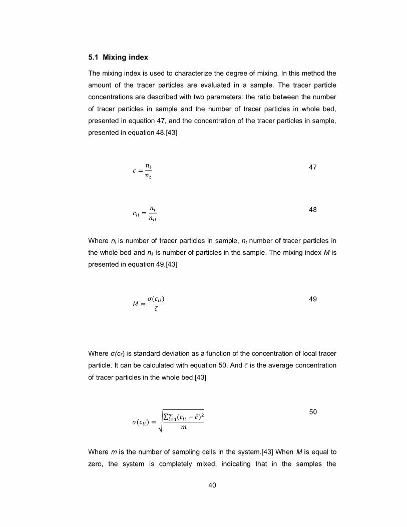
40
5.1 Mixing index
The mixing index is used to characterize the degree of mixing. In this method the
amount of the tracer particles are evaluated in a sample. The tracer particle
concentrations are described with two parameters: the ratio between the number
of tracer particles in sample and the number of tracer particles in whole bed,
presented in equation 47, and the concentration of the tracer particles in sample,
presented in equation 48.[43]
= 47
= 48
Where ni is number of tracer particles in sample, nt number of tracer particles in
the whole bed and nit is number of particles in the sample. The mixing index M is
presented in equation 49.[43]
=( )
49
Where σ(cli) is standard deviation as a function of the concentration of local tracer
particle. It can be calculated with equation 50. And is the average concentration
of tracer particles in the whole bed.[43]
( ) =∑ ( − )
50
Where m is the number of sampling cells in the system.[43] When M is equal to
zero, the system is completely mixed, indicating that in the samples the
41
concentration of the tracer particles is equal to the concentration of the tracer
particles in the whole system. The sample size must be large enough so that the
random errors will not affect the concentration calculations[44].
5.2 Mixing time
The time that is required to accomplish the complete mixing is called mixing time.
Euzen and Fortin, cited by Fan[1], wrote that the mixing time decreases when the
gas velocity is increasing. In addition, the rate of the decrease was significantly
higher for low liquid velocity than high liquid velocities.[1] In other words, the
complete mixing would be accomplished more quickly with higher gas velocities
and low liquid velocities.
6 Particle movement tracking
When assessing particle movement, there are invasive and non-invasive
measuring techniques. The invasive techniques are usually different kind of probes
that have been inserted in the flow region, which interferes with the flow and
hydrodynamics that could possibly lead to changes in the behavior of the system.
Invasive techniques are used more in the full scale industrial factories, because
the non-invasive measurement used in laboratory scale might not be sufficient for
running measurements deep in large industrial systems. In addition, the invasive
technologies are usually easier to apply and are often cheaper. Non-invasive
measuring techniques do not interfere with the system at all.[45]
When using the tracer particles in fluidization, it is important that properties of the
particles such as density, size, shape and surface properties to be nearly identical
with the other particles in the bed. In this way, the tracer particles would represent
all the other particles well.
Often the solid flow velocities and solid patterns are measured by observing the
movements of solid tracking particles. This method usually does not distinguish
single particles, but follow the particles as a mass. Nonetheless, it is usually more
useful to know how a single particle is moving and its residence time in different
parts of column.[46] The method where all the particles in the bed are tracked is
42
called tomography, while the tracking of single particle is simply called single
particle tracking.
Particles that are tracked are usually radioactive or optically detectable.
Radioactive particle tracking methods include positron emission particle tracking
(PEPT) and radioactive particle tracking (RPT), which is based on tracking gamma-
rays. Whereas, optically detectable particles can be tracked with analyzing videos
or photos, laser Doppler anemometry (LDA), particle image velocimetry (PIV), and
fluorescent particle image velocimetry (FPIV).[47] In addition to those mentioned
above, particle movement can be observed for example by following the movement
of ferromagnetic substances or particles with radio frequency identification tags
(RFID).
The optical tracking methods are usually used with refractive index matching
techniques. These techniques are used, for example, in laser Doppler velocimetry,
particle image velocimetry and photographic techniques. Refractive index
matching means that the refractive index of the column walls, the liquid and the
particles in bed are similarly matched. This enables the observation of the systems
without refraction errors.[48]
6.1 Positron emission particle tracking
In positron emission particle tracking (PEPT), the particle tracking is carried out by
following the gamma rays to locate the solid tracer particles containing positron
emitting substance. These tracers emits positron, which quickly annihilates with
electron to form two collinear gamma rays. These rays can be observed with
detectors outside the column. As the path of the rays are collinear, we can calculate
the line on which the particle is located. When another positron is emitted, another
line can be calculated and from those the location of the particle can be
triangulated. As the particle keeps emitting positrons as it moves by, the location
of the particle can be tracked.[46]
6.2 Radioactive particle tracking
One used method for tracking a single particle in fluidization is radioactive particle
tracking method (RPT). In this method a non-invasive single radioactive particle is
43
fed into the fluidized bed and then the emitted radiation is measured[12] for long
periods of time such as 8-12 hours.[49] This method is found to be a very reliable
techniques for investigating the movement of solid particles. Radioactive particle
tracking method can be utilized, for example, for quantification of the solid flow
structure, to obtain the solid flow velocity distributions, for evaluating the solids
mixing in the three-dimensional space and for mapping the solid velocity
vectors.[12]
Larachi et al. utilized the RPT system with eight NaI(Tl) detectors to measure the
emitted γ-rays in their studies. The data from all eight detectors were collected and
used for mapping the three-dimensional location of the particle. To be able to gain
useful location data from the detectors, the system needs to be calibrated every
time prior to measurements. This is done by positioning the particle in known
locations of the column.[12,49]
The tracer used in Larachi et al. experiments was a mixture of soda lime powder
and scandium oxide, which was melted at high temperature. The density of the
formed particle was rather close to the density of the glass particles used in the
fluidization experiments. The particle was then activated in a nuclear reactor.
emits γ-rays with energies of 889 and 1120 keV and the half-life of is 83.8
days.[49]
6.3 Imaging techniques
Different kinds of imaging techniques are usually used in observing and analyzing
the particle movements.[19,30,43,50] The imaging techniques has developed
greatly in recent years. When previously the cameras took a few picture per
seconds, nowadays cameras can take thousands of digital pictures per second
with great definition. This enables the image processing and obtaining of data with
different tools from the pictures to be considerably easier.
Imaging techniques requires a see-through column and can be used with the
refractive index matching techniques. Imaging techniques also requires an external
light source, so that the image sensor gets enough exposure. However, the
imaging is usually limited just to the particles in the vicinity of the walls[46].
44
6.4 Particle image velocimetry
Particle image velocimetry (PIV) is a technique that follows the particle movement
by taking pictures of the system. Lasers can be used as sources of light. PIV is
also used to examine the flow structure of gas or liquid with the help of seeding
particles[45].
PIV equipment normally includes four basic parts. The PIV measurements are
based on recording optically the movement of particles, so the first equipment
required for PIV is a recording device, normally a camera that takes pictures of the
system. A commonly used camera is the CCD camera. Other cameras include
cameras film or holographic cameras. Because in PIV the particles are followed
optically, the column has to be transparent in order for camera to be able to see
the particles in the column. The third piece of equipment needed is a light source,
so that the particles are illuminated enough for the camera. A frequently used light
source is the laser, the beam of which is reflected to form a pulsing “sheet” of light,
although, for larger particles, less powerful light source might be enough. The final
part of the PIV equipment needed is the image processing equipment, so that the
movement data can be extracted from the pictures.[51,52]
The tracer particles used in PIV needs to stand out optically from other particles in
the system. This can be accomplished for example by painting the tracer particles
with different colors so that the contrast difference would separate tracer particles
from the rest. Painting the tracer particle with fluorescent paint - so that the tracer
particle would emit light that can be identified – is another method in which to
highlight the tracer particles. Ideally the particles that are not been tracked would
be transparent so that they will not hinder the visibility of the tracer particles. Even
so, the problem with transparent particles might be that they refract the light, which
can disturb the tracer particle tracking to some extent.
Nowadays it is more common and more practical to use digital imaging instead of
the film photographic methods. Advantages of digital imaging include that the
image can be processed immediately, so that the feedback of the images can be
obtained immediately, and digital imaging has almost zero operating costs. Some
photographic film devices are still used due to high spatial resolution. Digital
imaging cameras commonly used in PIV are charge coupled devices (CCD),

45
charge injection devices (CID) or CMOS devices from which the CCD is the most
used.[52]
6.5 Three-dimensional particle tracking velocimetry
In studies done by Shirsat et al., three-dimensional particle tracking velocimetry
method were used. There, three high speed cameras recording the system
simultaneously. Images from the three camera were then processed and the three-
dimensional location of the particles obtained. In the Shirsat et al. experiments they
tracked 400 particles simultaneously. However, with different particle densities, the
amount could be greatly increased.[53]
6.6 Multiple color tracers
Mixing of solid particles can be observed by using multiple different color particles.
Different color particles are set to the column layer by layer so that in one layer
there are same color particles. This method gives information on how the particles
have been mixed from the starting point. Drawback from this method is that data
regarding the mixing is challenging to obtain during the mixing. Boyer et
al.[45]:p3190 states that this kind of method was used in Fortin’s experiments.
Zhang et al. used multiple color tracers with two different color particles. The
different colored particles were set in in two layer. The first layer was 9 cm high
and, above that, another 1 cm high layer of different color particles were set. Then
the fluid flow to the bed was started. In a certain time the flashboard box was
instantaneously inserted to the bed from the top. The box divided the bed into radial
sections. The fluid flow was simultaneously shut down. Afterwards that the number
of the tracer particles in different sectors were counted.[43] With this method it is
was possible to see how the particles are distributed radially in the column.
6.7 Magnetic particle tracking
A rather new method for tracking solid particles is magnetic particle tracking (MPT).
In this method single magnetic particle is tracked with multiple sensors, which
measure the magnetic field generated by magnetic particles. The signals produced
are used to calculate the particle location.[54]
46
An advantage of this method compared to radioactive tracers (PEPT and RPT) is
the low cost since in PEPT and RPT the cost of the sensors and the cost of
handling, preparing as well as using the radioactive material is considerably high.
Furthermore, the safety issues due malhandling radioactive material cannot be
overlooked. When comparing to magnetic particle tracking to imaging methods the
advantage of magnetic particle tracking is that it is more easily adaptable to three
dimensional systems.[54]
Avidan and Yerushalmi utilized the magnetic tracer tracking in their experiments.
They injected magnetic tracer particles into fluidized bed, so that from all the bed
particles 0.5% were tracers. The tracers were observed with four external probes
that gave impulses that were translated to tracer concentration in the cross-section
of the column.[55]
6.8 Thermal tracer tracking
Valenzuela and Glicksman used heated tracer particles that were tracked with
multiple thermocouples. In this method, the particles were heated prior to inserting
them into the bed. Particles are cooled down in minutes subsequent to insertion,
so the experiments had to be repeated many times in order to obtain
comprehensive data.[56]
Glicksman et al. used similar method but with cooled particles. Tracer particles
were cooled to temperatures 100 degrees below the bed temperature with liquid
nitrogen. After the particles had cooled down they were inserted into the bed. The
particles were then traced with thermistors mounted on within the column. The
particles were monitored 10 seconds subsequent to the insertion and because the
particles were identical to bed particles there was no need to separate the tracers
afterwards. Because of the short experiment times, the experiments must be
repeated.[57]
Zhang et al. developed a technique that uses an infrared camera to track particles
while the tracer particles are heated simultaneously with microwaves. The tracer
particles were made of silicon carbide. Particles were observed with infrared video-
camera through infrared permeable glass combined with a microwave blocking
shield. The video was then processed and the particle movement data obtained

47
with computers.[41] This method is not suitable for systems containing polarized
material like water.
48
Experimental part
7 Experimental setup
The column used in experiments is made of see-through Plexiglas and its height
is 1.7 meter of which 1.2 meter is above the distribution plate. Cross-sectional
shape of the column is square with internal dimensions of 0.1 m * 0.1 m. The
distribution plate is perforated plate having 5 mm diameter holes with open area of
35 % and above the plate there is a small wire mesh. Column has Bürkert 8314
pressure transmitters with 25 cm intervals throughout the height of the column.
In addition to the column, the experiment equipment consists three subsystems,
liquid feed, air feed, and data acquisition system. The liquid feed system includes
liquid tank, pump and flow meter. The liquid tank is 300 liter in size with two inlet
pipes near the top of the tank and one outlet pipe to the pump in the bottom of the
tank. The tank has opening hatch on the top. The pump used is Ebara 3LM4
centrifugal pump. The flow velocity to the column is adjusted with two valves
subsequent to the pump. One of the valves regulates the feed to the column and
the second valve regulates the minimum circulation flow of the pump. Between the
liquid feed valve and the column there is a liquid flow meter measuring the flow
going to column. Liquid is fed through the flowmeter to the column from the bottom.
The schematic diagram of the column is presented in Figure 8.
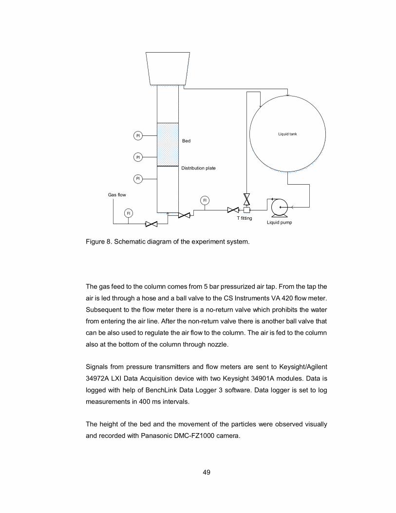
49
Distribution plate
Liquid tank
Gas flow
Liquid pumpT fitting
Bed
FI
FI
PI
PI
PI
Figure 8. Schematic diagram of the experiment system.
The gas feed to the column comes from 5 bar pressurized air tap. From the tap the
air is led through a hose and a ball valve to the CS Instruments VA 420 flow meter.
Subsequent to the flow meter there is a no-return valve which prohibits the water
from entering the air line. After the non-return valve there is another ball valve that
can be also used to regulate the air flow to the column. The air is fed to the column
also at the bottom of the column through nozzle.
Signals from pressure transmitters and flow meters are sent to Keysight/Agilent
34972A LXI Data Acquisition device with two Keysight 34901A modules. Data is
logged with help of BenchLink Data Logger 3 software. Data logger is set to log
measurements in 400 ms intervals.
The height of the bed and the movement of the particles were observed visually
and recorded with Panasonic DMC-FZ1000 camera.

50
8 Operation principle
Objective of the experiments is to observe behavior and behavior changes with
different gas flow and liquid flow rates. The experiments are carried out by
adjusting flows with adjustable valves meanwhile pressure data in the column and
flow velocity data are logged. In addition, particles, bubble and flow behaviors are
observed both visually and recorded with camera.
9 Used materials
In the fluidization column there are gas, liquid and solid phases present. In these
experiments the gas phase is pressurized air, liquid phase is tap water and solid
particles are glass beads.
9.1 Solid particles
In the bed there are 6439.6 g SiLibeads glass particles with diameters varying from
2.0 to 2.5 mm. Less than 0.5 % of the particles are painted red, in order to ease
the observing of the movement of the particles. The particles are all assumed to
be spheres. The average wet density of the particles is 2471.1 g/l.
The tracer beads were painted with red spray-paint. The beads were set evenly on
a flat surface and then spray-paint was applied evenly. When the particles had
dried they were mixed and the painting procedure was repeated a few times in
order to assure that all the sides of the beads were painted. Then the painted beads
were let to dry for five days. The used spray-paint was Maston 805 RAL 3000 Red.
Mass of a single particle was determined by weighting 100 particles and assuming
that they were representing all the particles in the bed. Average weight of one
particle was 0.01505 grams, so that in one kilogram there are 66 450 particles.
When the mass of the particles in the bed is known we can calculate that there are
427 900 beads in the bed.
Particle size was analyzed by measuring the particle diameter with Vernier caliper.
Average diameter for 100 measured particles was 2.27 mm with standard deviation

51
of 0.108 mm. The particle size distribution is presented in Figure 9. All the particles
were not exactly spherical however close enough to assume them to be.
Figure 9. Particle diameter distribution.
The skeletal density of the particles were measured by a 250 ml volumetric flask.
The empty volumetric flask was first weighed. Then to the flask was added certain
amount of beads and then flask was weighed again. After that the volumetric flask
was filled with 20 °C water until the 250 ml mark in the flask and then once again
the flask was weighed. Then the skeletal density of the particles were calculated
from the weight and the volume of the particles. Skeletal densities were defined
with three different measurements for colorless beads and once with red particles.
= , − = 364.13 − 92.76
= 271.37
0
1
2
3
4
5
6
7
8
9
19.8 20
20.2
20.4
20.6
20.8 21
21.2
21.4
21.6
21.8 22
22.2
22.4
22.6
22.8 23
23.2
23.4
23.6
23.8 24
24.2
24.4
24.6
24.8
Freq
uenc
y
Particle diameter [10-1 mm]
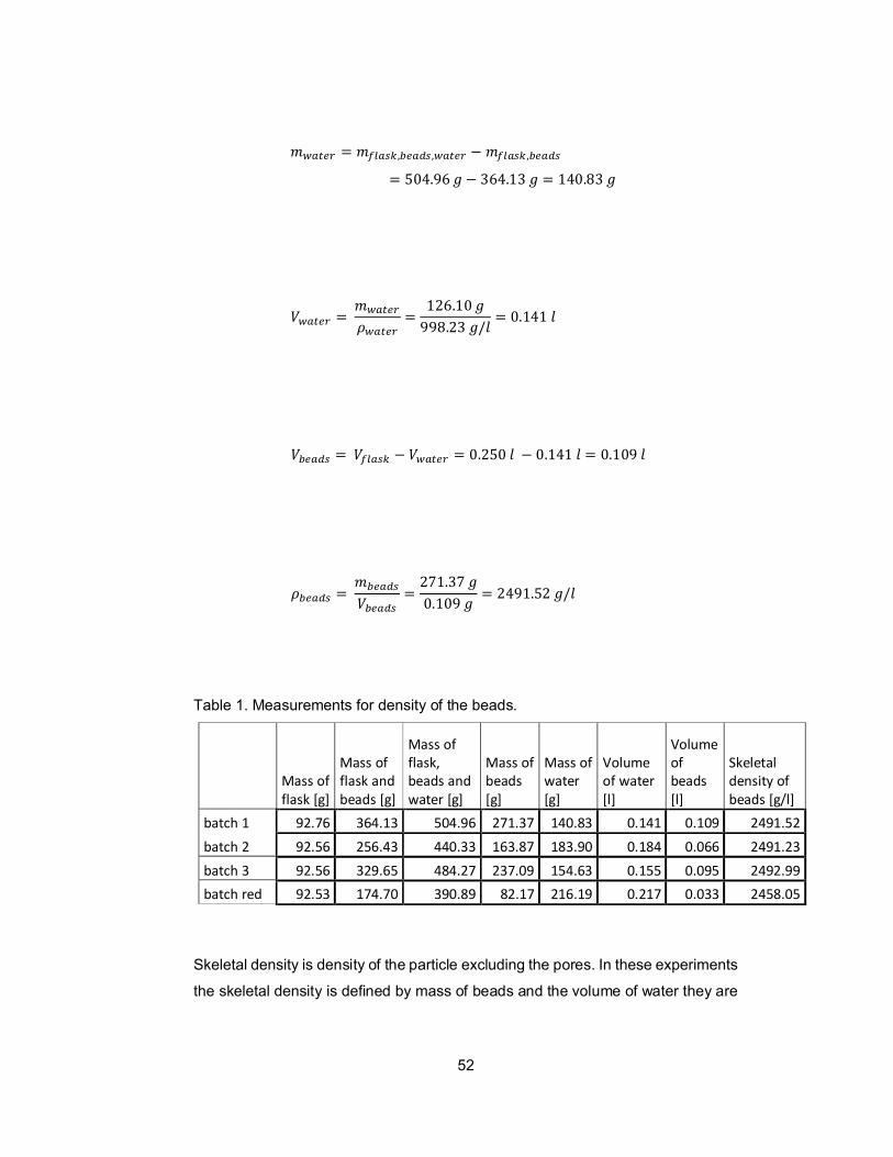
52
= , , − ,
= 504.96 − 364.13 = 140.83
= =126.10
998.23 /= 0.141
= − = 0.250 − 0.141 = 0.109
= =271.370.109
= 2491.52 /
Table 1. Measurements for density of the beads.
Mass offlask [g]
Mass offlask andbeads [g]
Mass offlask,beads andwater [g]
Mass ofbeads[g]
Mass ofwater[g]
Volumeof water[l]
Volumeofbeads[l]
Skeletaldensity ofbeads [g/l]
batch 1 92.76 364.13 504.96 271.37 140.83 0.141 0.109 2491.52batch 2 92.56 256.43 440.33 163.87 183.90 0.184 0.066 2491.23batch 3 92.56 329.65 484.27 237.09 154.63 0.155 0.095 2492.99batch red 92.53 174.70 390.89 82.17 216.19 0.217 0.033 2458.05
Skeletal density is density of the particle excluding the pores. In these experiments
the skeletal density is defined by mass of beads and the volume of water they are

53
replacing. Average skeletal density for clear beads is 2491.91 g/l and weighted
average for all the beads in the bed is 2490.8 g/l.
There are 66 450 particles in one kilogram so the number of particles in one batch
can be calculated as follows.
= ∙
= 0.27137 ∙ 66450 = 18033
If all particles are presumed fully spherical(nonporous) volume of beads can be
calculated as follows.
= ∙34
2
= 18033 ∙34
∙0.00227
2
∙ 1000 = 0.110
With volume of nonporous beads and measured skeletal volume of the beads the
void fraction can be calculated. This void fraction describes the volume difference
between fully spherical bead and measured bead.
=
= . .
. = 0.0138
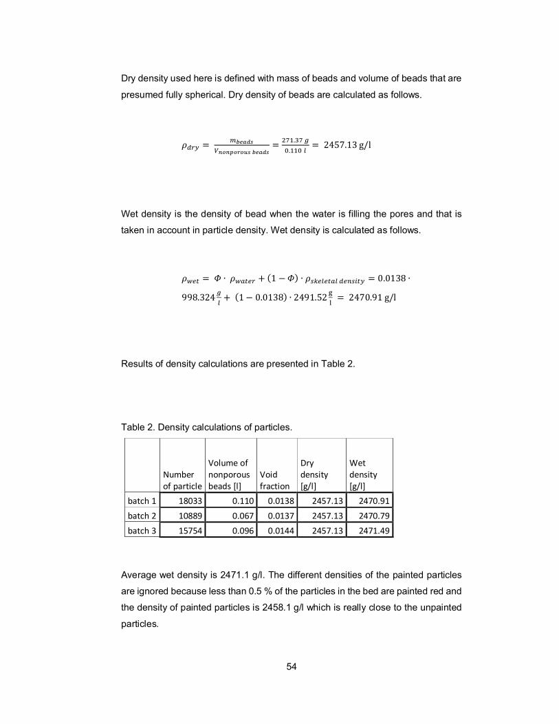
54
Dry density used here is defined with mass of beads and volume of beads that are
presumed fully spherical. Dry density of beads are calculated as follows.
=
= . .
= 2457.13g/l
Wet density is the density of bead when the water is filling the pores and that is
taken in account in particle density. Wet density is calculated as follows.
= ∙ + (1 − ) ∙ = 0.0138 ∙
998.324 + (1− 0.0138) ∙ 2491.52 = 2470.91g/l
Results of density calculations are presented in Table 2.
Table 2. Density calculations of particles.
Numberof particle
Volume ofnonporousbeads [l]
Voidfraction
Drydensity[g/l]
Wetdensity[g/l]
batch 1 18033 0.110 0.0138 2457.13 2470.91batch 2 10889 0.067 0.0137 2457.13 2470.79batch 3 15754 0.096 0.0144 2457.13 2471.49
Average wet density is 2471.1 g/l. The different densities of the painted particles
are ignored because less than 0.5 % of the particles in the bed are painted red and
the density of painted particles is 2458.1 g/l which is really close to the unpainted
particles.

55
9.2 Liquid phase
The liquid phase used in the experiments is tap water at temperatures varying
between 14 – 19 °C.
9.3 Gas phase
The gas phased used in the experiments is pressurized air obtained from 5 bar
compressed air line. The air is dried prior to compressing it into 5 bar and fed to
the line.
10 Testing equipment installment
The experiments required installation of new equipment to the existing testing
setup. This new equipment included new data logging equipment and new gas and
liquid flowmeters.
10.1 Data logging equipment installment
New data logging equipment is Keysight/Agilent 34972A LXI Data Acquisition
device. In order to obtain the data from the pressure sensors and flow meters an
exterior power supply is needed. Before the experiments all the wiring between
meters, power supply and data logger were connected. All the meters were
connected with two wire connections where the power supply and the transmitter
were connected in circuit as illustrated in Figure 10.
DC Transmitter
Current meter
Figure 10. Wiring diagram of transmitters.
56
10.2 Gas flowmeter installment
The gas flow meter was installed in pipeline with equalizing sections prior to and
subsequent to the sensor. Pressurized air was fed from tap along 10 mm inside
diameter hose. Hose was connected to the pipe where the flow sensor was
installed. The pipe was connected to the column with similar hose used to connect
the tap and flow meter pipe. Shut-off valves were installed prior to and subsequent
to the pipe section and additionally subsequent to the pipe also non-return valve
was installed to prevent water entering the gas flow section.
10.3 Liquid flow meter installment
Liquid flow meter was attached to 40 cm long inlet and outlet pipes. The pipes were
connected with 38 mm inside diameter hose to the pump and to the valves that
regulates the water flow rate to the column.
During the experiments it was observed that valves regulating the flow velocities
generated unwanted disturbance in the liquid flow. In addition, the pump is not
running in optimal range which also might produce some disturbance in the flow.
The flow became slightly pulse-like causing additional rocking motion in particles
and scatter in pressure measurements. This disturbance could be decreased by
closing the valve for liquid minimum circulation flow. However this valve cannot be
fully closed with low liquid velocities to the column because of the stress resulting
for the pump.
11 Results
11.1 Minimum fluidization
Minimum fluidization point were measured by first setting the liquid flow to around
0.075 m/s and then starting the data logging. Then the liquid flow velocity was
decreased gradually until the flow was noticeably smaller than visually observed
minimum fluidization point.
Minimum fluidization point was defined in these experiments with two pressure
sensors 25 cm from each other within the bed. The exact minimum fluidization

57
point was determined by plotting the pressure drop between the two sensors as a
function of the flow velocity. The point where the slope of pressure drop changes
is minimum fluidization point. When the superficial liquid flow velocity was defined
at minimum fluidization point new measurement for pressure drop and bed height
was carried out. The superficial liquid flow velocity was set in constant flow at
minimum fluidization point. Then the pressure difference and bed height was
measured.
It is worth mentioning that when the pressure drop is measured in two fixed points
within the bed, it is required for the calculations to assume that in the whole bed
the particles are homogenously distributed. In reality this might not be exactly true
since for example near the top of the bed the particle distribution is more uneven
and sparse due to bubble interaction and particles thrown into freeboard region.
Especially with higher gas flows the pressure drop – superficial liquid velocity
curves from raw data disperse considerably, so that the graphs are really
challenging to interpret without data processing as seen in Figure 11.
Figure 11. Pressure drop as a function of superficial liquid flow velocity from rawdata. Superficial gas flow velocity is 0.034 m/s.
0.03
0.035
0.04
0.045
0.05
0.055
0.06
0.065
0.00 0.01 0.02 0.03 0.04 0.05 0.06 0.07 0.08
Δp[b
ar]
Ul [m/s]

58
When averaging nine consequent pressure drop and superficial liquid flow velocity
measurements the dispersion decreases to some extent. Graph made from these
values is presented in Figure 12 with superficial gas velocity of 3.4 cm/s.
Figure 12. Pressure drop as function of superficial liquid flow velocity from 9averaged data points.
Data points were divided into groups by superficial liquid flow velocity in 0.001 m/s
intervals and taking median of the pressure drops belonging to each group. The
median presented pressure drop of each group. By plotting the group median
pressure drop as function of intermediate superficial liquid flow velocity value of
each group slightly less dispersed graph is formed as seen in Figure 13.
0.03
0.035
0.04
0.045
0.05
0.055
0 0.01 0.02 0.03 0.04 0.05 0.06 0.07 0.08
Δp[b
ar]
Ul [m/s]

59
Figure 13. Pressure drop as function of superficial liquid flow velocity with groupingsuperficial flow velocities.
This grouping method was used to specify the minimum fluidization points i.e. the
points where the trend in the each graph changes. The minimum fluidization points
were defined with six different gas velocities.
The graph in Figure 14 illustrates superficial velocities of gas and liquid at the
minimum fluidization. It is seen in the Figure 14. Superficial velocities at minimum
fluidization. It can be seen in the Figure 14 that at the minimum fluidization point
the superficial liquid velocity is considerably higher when there is no gas flow or
diminutive small gas flow. When the superficial gas flow is higher the superficial
liquid velocity at minimum fluidization is rather independent on gas flow rate.
0.03
0.035
0.04
0.045
0.05
0.055
0 0.005 0.01 0.015 0.02 0.025 0.03 0.035 0.04 0.045 0.05 0.055 0.06
Δp[b
ar]
Ul [m/s]
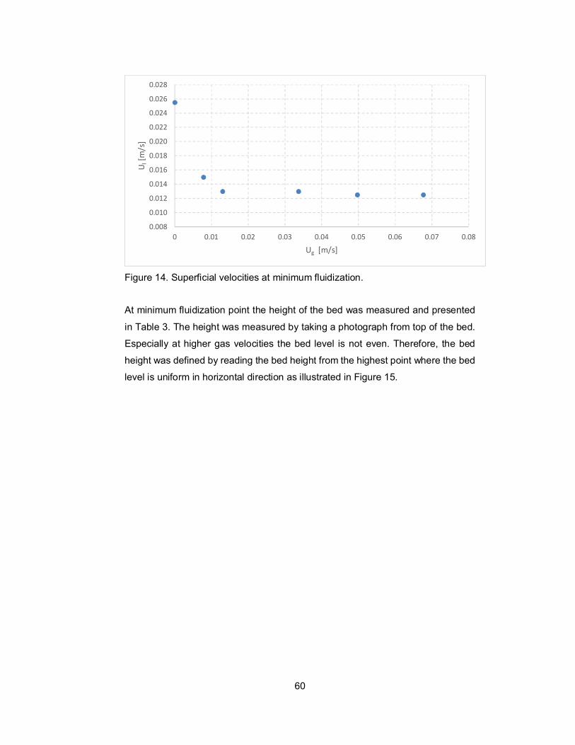
60
Figure 14. Superficial velocities at minimum fluidization.
At minimum fluidization point the height of the bed was measured and presented
in Table 3. The height was measured by taking a photograph from top of the bed.
Especially at higher gas velocities the bed level is not even. Therefore, the bed
height was defined by reading the bed height from the highest point where the bed
level is uniform in horizontal direction as illustrated in Figure 15.
0.008
0.010
0.012
0.014
0.016
0.018
0.020
0.022
0.024
0.026
0.028
0 0.01 0.02 0.03 0.04 0.05 0.06 0.07 0.08
U l[m
/s]
Ug [m/s]
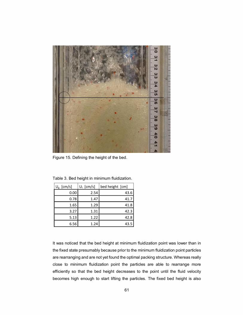
61
Figure 15. Defining the height of the bed.
Table 3. Bed height in minimum fluidization.
Ug [cm/s] Ul [cm/s] bed height [cm]0.00 2.54 43.60.78 1.47 41.71.65 1.29 41.83.27 1.31 42.35.13 1.22 42.86.56 1.24 43.5
It was noticed that the bed height at minimum fluidization point was lower than in
the fixed state presumably because prior to the minimum fluidization point particles
are rearranging and are not yet found the optimal packing structure. Whereas really
close to minimum fluidization point the particles are able to rearrange more
efficiently so that the bed height decreases to the point until the fluid velocity
becomes high enough to start lifting the particles. The fixed bed height is also

62
dependent on how the expanded bed is lowered to fixed state. If the bed is
collapsed the fixed bed height is higher than if it is taken down slowly by increasing
fluid flow gradually. The bed that has been gradually taken down the fixed bed
height is close to height of the bed at minimum fluidization point. The difference
was more than 1 % of the bed height and slightly more than 2 % in solid hold up.
11.2 Hold-ups
Hold-ups express the fraction of specific phase in cross-section of the column. For
calculating the solids and gas hold-up equations 10, 11, 12, 13, and 14 were used.
11.2.1 Solids hold-up
When the mass of the particles in the bed, the density of the particles, the cross-
section area of the column, and the height of the bed is known the solids hold-up
can be calculated with equation 10.
It was discovered that the bed height measurements are not that straightforward
and unambiguous since remarkable amount of particles are entrained into
freeboard region especially with higher gas flow rates. So visually determining the
height of the bed accurately is really challenging.
The height of the bed at minimum fluidization point were measured in different gas
velocities. The solids hold-up was then calculated at the minimum fluidization point
at different gas velocities.
The mass of the bed was weighted prior to inserting the particles into the column.
The density of the particles and the cross-section area of the column was known
and the height of the bed was measured from the photographs.
, = =6439.6
2471.1 ∙ 0.01 ∙ 0.436= 0.598
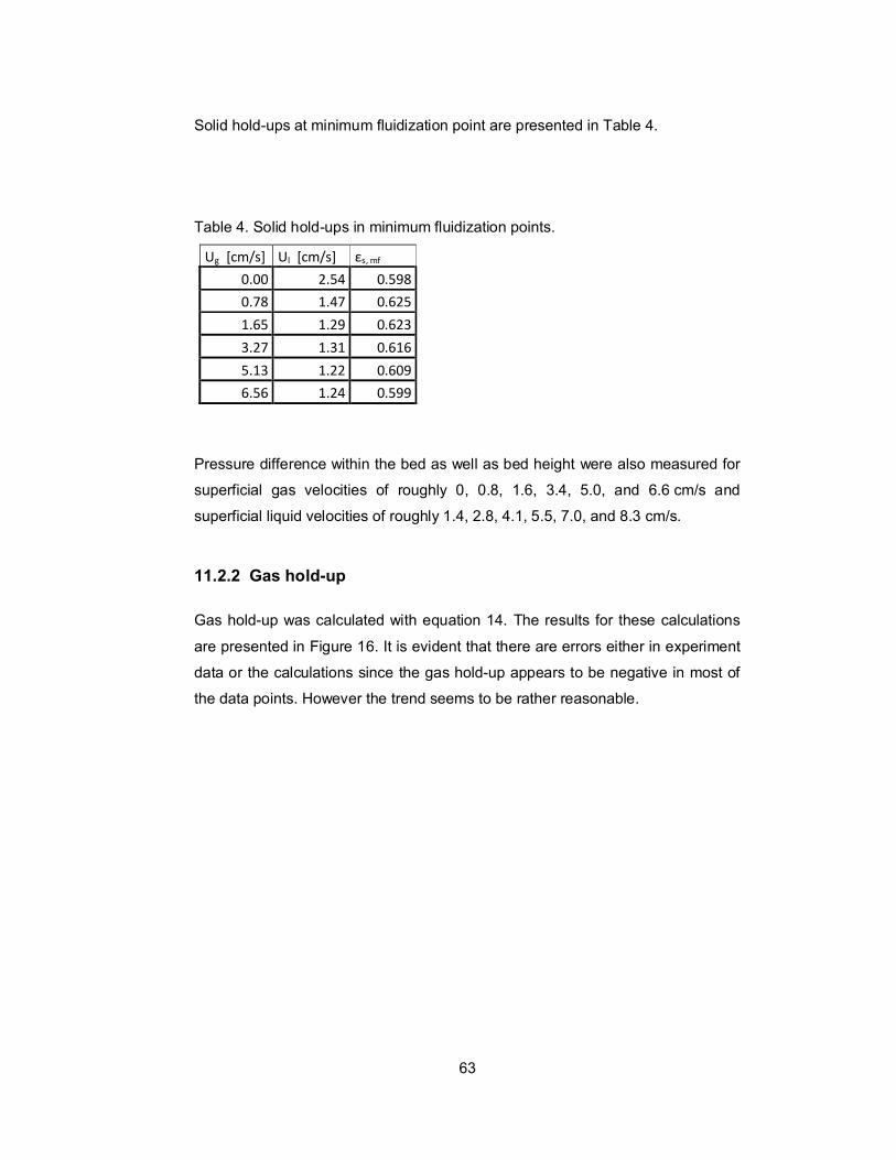
63
Solid hold-ups at minimum fluidization point are presented in Table 4.
Table 4. Solid hold-ups in minimum fluidization points.
Ug [cm/s] Ul [cm/s] εs, mf
0.00 2.54 0.5980.78 1.47 0.6251.65 1.29 0.6233.27 1.31 0.6165.13 1.22 0.6096.56 1.24 0.599
Pressure difference within the bed as well as bed height were also measured for
superficial gas velocities of roughly 0, 0.8, 1.6, 3.4, 5.0, and 6.6 cm/s and
superficial liquid velocities of roughly 1.4, 2.8, 4.1, 5.5, 7.0, and 8.3 cm/s.
11.2.2 Gas hold-up
Gas hold-up was calculated with equation 14. The results for these calculations
are presented in Figure 16. It is evident that there are errors either in experiment
data or the calculations since the gas hold-up appears to be negative in most of
the data points. However the trend seems to be rather reasonable.
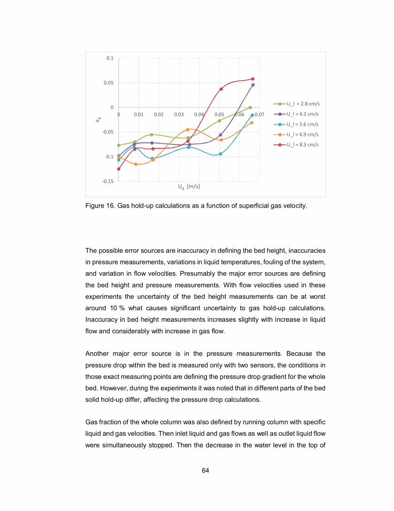
64
Figure 16. Gas hold-up calculations as a function of superficial gas velocity.
The possible error sources are inaccuracy in defining the bed height, inaccuracies
in pressure measurements, variations in liquid temperatures, fouling of the system,
and variation in flow velocities. Presumably the major error sources are defining
the bed height and pressure measurements. With flow velocities used in these
experiments the uncertainty of the bed height measurements can be at worst
around 10 % what causes significant uncertainty to gas hold-up calculations.
Inaccuracy in bed height measurements increases slightly with increase in liquid
flow and considerably with increase in gas flow.
Another major error source is in the pressure measurements. Because the
pressure drop within the bed is measured only with two sensors, the conditions in
those exact measuring points are defining the pressure drop gradient for the whole
bed. However, during the experiments it was noted that in different parts of the bed
solid hold-up differ, affecting the pressure drop calculations.
Gas fraction of the whole column was also defined by running column with specific
liquid and gas velocities. Then inlet liquid and gas flows as well as outlet liquid flow
were simultaneously stopped. Then the decrease in the water level in the top of
-0.15
-0.1
-0.05
0
0.05
0.1
0 0.01 0.02 0.03 0.04 0.05 0.06 0.07
ε g
Ug [m/s]
U_l = 2.8 cm/s
U_l = 4.2 cm/s
U_l = 5.6 cm/s
U_l = 6.9 cm/s
U_l = 8.3 cm/s
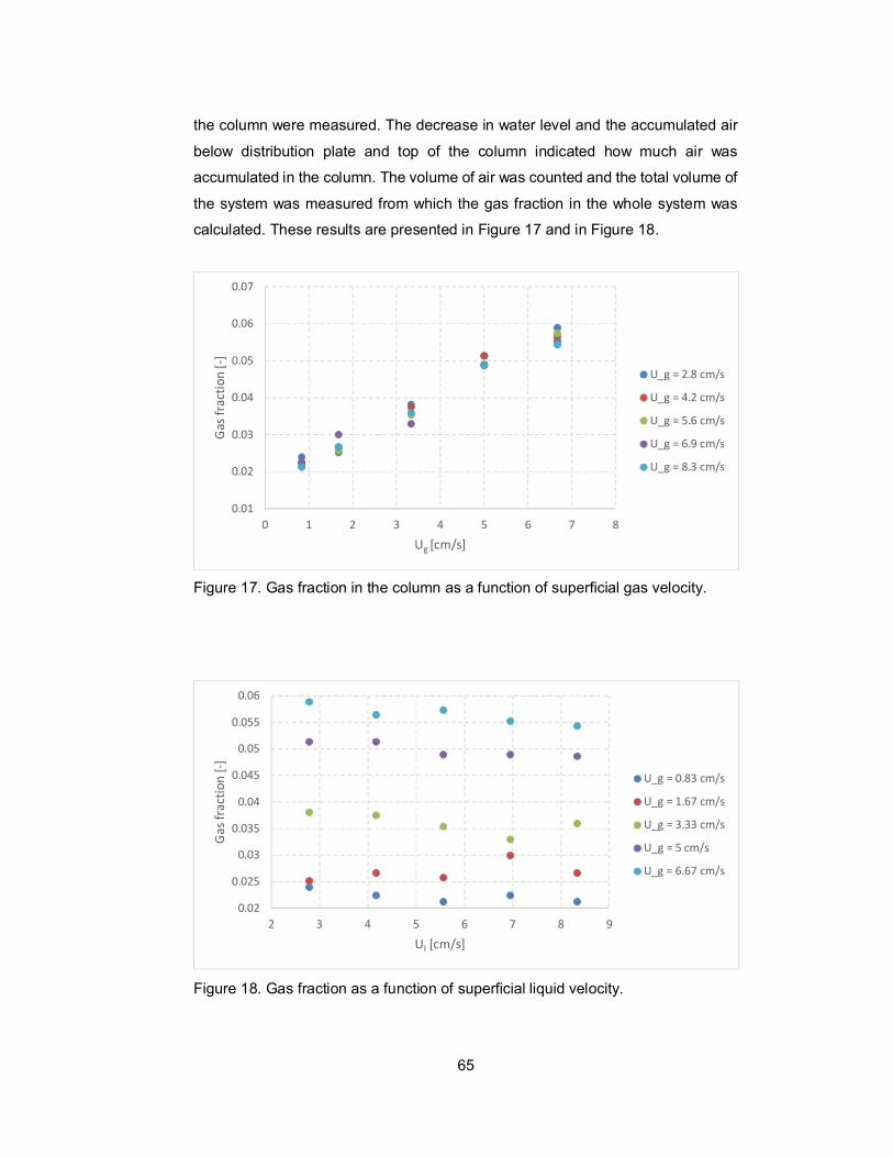
65
the column were measured. The decrease in water level and the accumulated air
below distribution plate and top of the column indicated how much air was
accumulated in the column. The volume of air was counted and the total volume of
the system was measured from which the gas fraction in the whole system was
calculated. These results are presented in Figure 17 and in Figure 18.
Figure 17. Gas fraction in the column as a function of superficial gas velocity.
Figure 18. Gas fraction as a function of superficial liquid velocity.
0.01
0.02
0.03
0.04
0.05
0.06
0.07
0 1 2 3 4 5 6 7 8
Gas
frac
tion
[-]
Ug [cm/s]
U_g = 2.8 cm/s
U_g = 4.2 cm/s
U_g = 5.6 cm/s
U_g = 6.9 cm/s
U_g = 8.3 cm/s
0.02
0.025
0.03
0.035
0.04
0.045
0.05
0.055
0.06
2 3 4 5 6 7 8 9
Gas
frac
tion
[-]
Ul [cm/s]
U_g = 0.83 cm/s
U_g = 1.67 cm/s
U_g = 3.33 cm/s
U_g = 5 cm/s
U_g = 6.67 cm/s
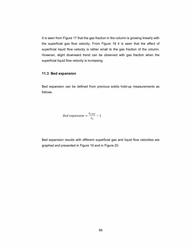
66
It is seen from Figure 17 that the gas fraction in the column is growing linearly with
the superficial gas flow velocity. From Figure 18 it is seen that the effect of
superficial liquid flow velocity is rather small to the gas fraction of the column.
However, slight downward trend can be observed with gas fraction when the
superficial liquid flow velocity is increasing.
11.3 Bed expansion
Bed expansion can be defined from previous solids hold-up measurements as
follows.
= , − 1
Bed expansion results with different superficial gas and liquid flow velocities are
graphed and presented in Figure 19 and in Figure 20.
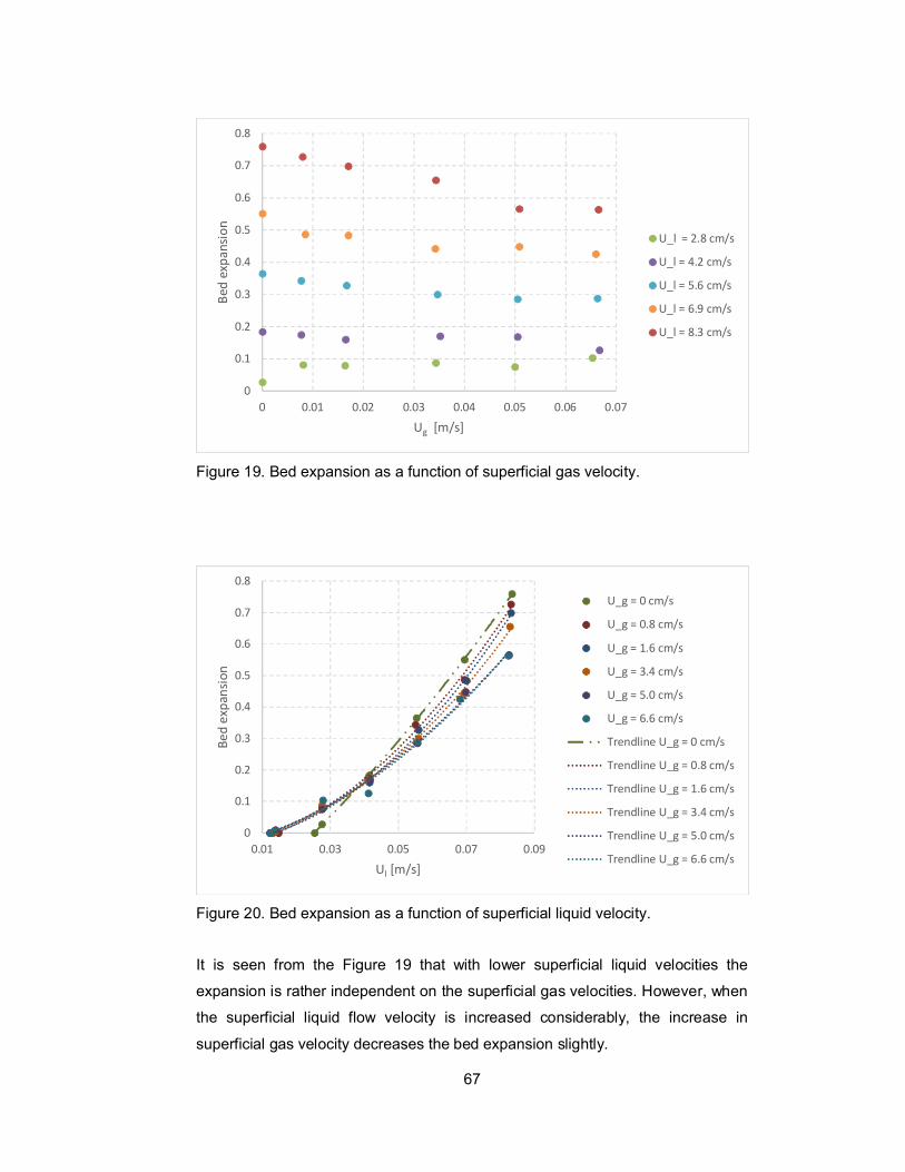
67
Figure 19. Bed expansion as a function of superficial gas velocity.
Figure 20. Bed expansion as a function of superficial liquid velocity.
It is seen from the Figure 19 that with lower superficial liquid velocities the
expansion is rather independent on the superficial gas velocities. However, when
the superficial liquid flow velocity is increased considerably, the increase in
superficial gas velocity decreases the bed expansion slightly.
0
0.1
0.2
0.3
0.4
0.5
0.6
0.7
0.8
0 0.01 0.02 0.03 0.04 0.05 0.06 0.07
Bed
expa
nsio
n
Ug [m/s]
U_l = 2.8 cm/s
U_l = 4.2 cm/s
U_l = 5.6 cm/s
U_l = 6.9 cm/s
U_l = 8.3 cm/s
0
0.1
0.2
0.3
0.4
0.5
0.6
0.7
0.8
0.01 0.03 0.05 0.07 0.09
Bed
expa
nsio
n
Ul [m/s]
U_g = 0 cm/s
U_g = 0.8 cm/s
U_g = 1.6 cm/s
U_g = 3.4 cm/s
U_g = 5.0 cm/s
U_g = 6.6 cm/s
Trendline U_g = 0 cm/s
Trendline U_g = 0.8 cm/s
Trendline U_g = 1.6 cm/s
Trendline U_g = 3.4 cm/s
Trendline U_g = 5.0 cm/s
Trendline U_g = 6.6 cm/s

68
In Figure 20 it is seen that the bed expansion as a function of superficial liquid
velocity follows well the polynomic fittings. Another observation from the expansion
measurements is that the bed expansion seems to behave differently when there
is gas flow to the column compared to the situation where there is only liquid flow.
When there is only liquid flow the minimum fluidization point is later than with gas
and liquid flow. However, the expansion increases faster when gas flow is not
introduced. In consequence there is a point where the bed expansion curves for
liquid-gas systems and liquid system are crossing. Nevertheless, the uncertainties
in the measurements of the bed height can partly explain these results.
11.4 Particle movement
Particle movement was observed with a video camera in one side of the column.
Recording only from one side posed a problem since it was noticed that the flow
patterns near the walls were not similar in all sides of the column. By comparing
the different sides of the column, channeling could be clearly observed.
Consequently, with these methods flow and particle moving patterns could not be
comprehensively analyzed even at the vicinity of the column walls.
In the experiments considerable channeling was noticed regardless of the liquid or
gas flow velocities. The channeling was observed near the minimum fluidization
velocities as well as with much higher fluid flow velocities. When approaching the
minimum fluidization point while increasing the fluid flow velocities the particles first
started to move in one part of the column cross-section and when increasing the
fluid flow velocity further, the particles started to move in all parts of the cross-
section and in the channeling parts the movement was considerably faster.
Channeling was likely due to the distribution plate design and other column design
aspects.
11.4.1 Liquid-solid fluidization
At minimum fluidization point minor particle rocking movement was observed with
the particles on the top of the bed as well as just above the distribution plate. When
the flow velocity was increased, broader movement of particles was observed. The
particles just above the distribution plate were carried up short distances in fluid
flow by the walls in center parts of the sides. When particles reached their highest

69
position they were then pushed to corners and central parts of the column where
they started slowly descending as illustrated in Figure 21. In upper parts of the
column the particles were moving considerably slower than in the lower parts of
the column near the distribution plate.
Figure 21. Particle flow pattern above the minimum fluidization point.
When the liquid flow velocities were increased, the flow pattern seemed to alter
slightly. Particles still seemed to have greater upward velocity near the distribution
plate by the walls in center parts of the sides however after traveling short
distances the rapidly upward moving particles were shifted towards corners where
they continued moving rapidly upwards as illustrated in Figure 22. Since the flow
was rather channeled, considerable turbulent motion of the particles were
observed.

70
Figure 22. Particle flow pattern at higher superficial liquid flow velocities.
With slower liquid velocities the rapid particle movement was limited to the lower
parts of the column. However, when the liquid flow velocity was increased also the
particles in the higher parts of the column started to move more rapidly.
When the particle movement in the bed was observed with bright light behind the
column, variations in particle density within the bed was observed. As seen in
Figure 23 the density variation is seen as brighter horizontal lines in the bed. The
density variations in the bed were moving upwards in the bed. New density
variations in the bed are forming continuously near the distribution plate.
This wavelike motion phenomena was observed more strongly with higher liquid
flow velocities but was also observed with lower liquid velocities. When the gas
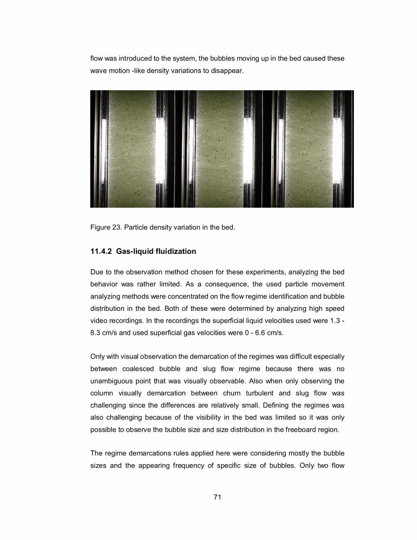
71
flow was introduced to the system, the bubbles moving up in the bed caused these
wave motion -like density variations to disappear.
Figure 23. Particle density variation in the bed.
11.4.2 Gas-liquid fluidization
Due to the observation method chosen for these experiments, analyzing the bed
behavior was rather limited. As a consequence, the used particle movement
analyzing methods were concentrated on the flow regime identification and bubble
distribution in the bed. Both of these were determined by analyzing high speed
video recordings. In the recordings the superficial liquid velocities used were 1.3 -
8.3 cm/s and used superficial gas velocities were 0 - 6.6 cm/s.
Only with visual observation the demarcation of the regimes was difficult especially
between coalesced bubble and slug flow regime because there was no
unambiguous point that was visually observable. Also when only observing the
column visually demarcation between churn turbulent and slug flow was
challenging since the differences are relatively small. Defining the regimes was
also challenging because of the visibility in the bed was limited so it was only
possible to observe the bubble size and size distribution in the freeboard region.
The regime demarcations rules applied here were considering mostly the bubble
sizes and the appearing frequency of specific size of bubbles. Only two flow
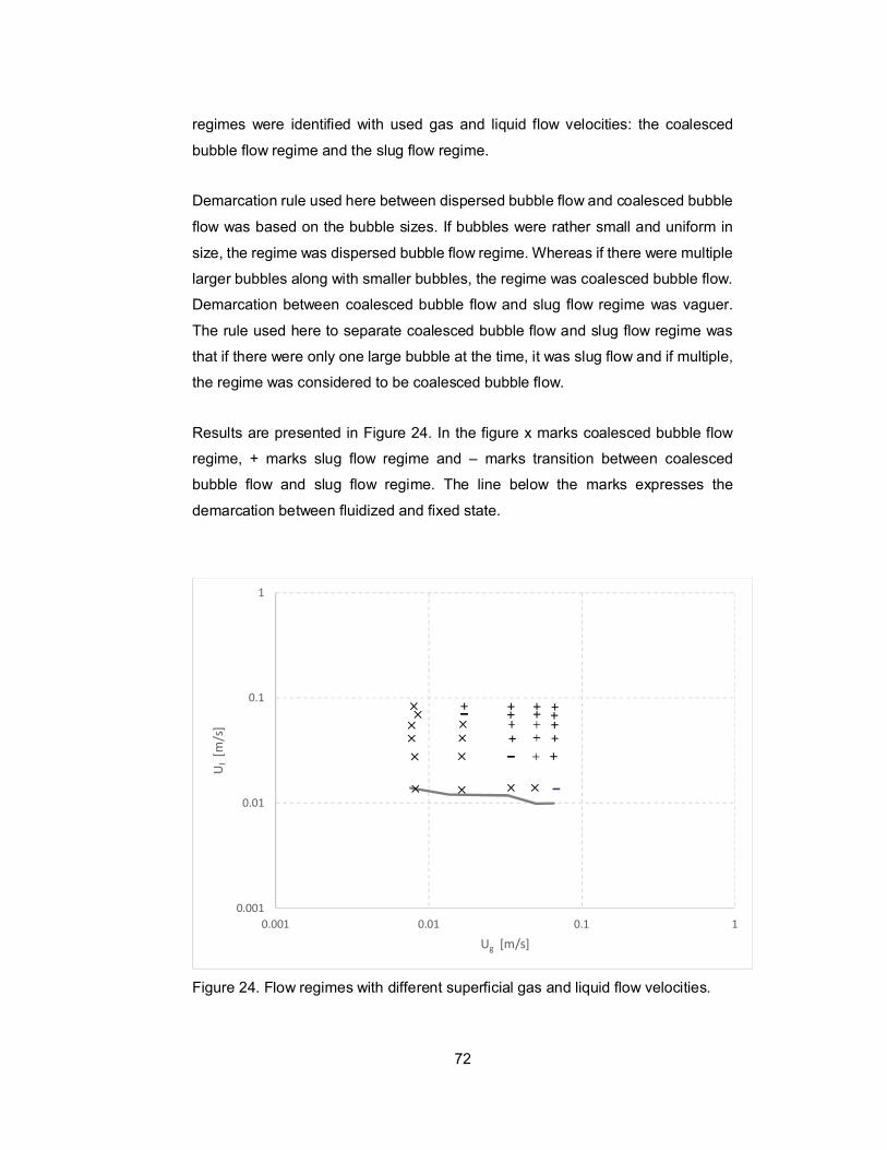
72
regimes were identified with used gas and liquid flow velocities: the coalesced
bubble flow regime and the slug flow regime.
Demarcation rule used here between dispersed bubble flow and coalesced bubble
flow was based on the bubble sizes. If bubbles were rather small and uniform in
size, the regime was dispersed bubble flow regime. Whereas if there were multiple
larger bubbles along with smaller bubbles, the regime was coalesced bubble flow.
Demarcation between coalesced bubble flow and slug flow regime was vaguer.
The rule used here to separate coalesced bubble flow and slug flow regime was
that if there were only one large bubble at the time, it was slug flow and if multiple,
the regime was considered to be coalesced bubble flow.
Results are presented in Figure 24. In the figure x marks coalesced bubble flow
regime, + marks slug flow regime and – marks transition between coalesced
bubble flow and slug flow regime. The line below the marks expresses the
demarcation between fluidized and fixed state.
Figure 24. Flow regimes with different superficial gas and liquid flow velocities.
0.001
0.01
0.1
1
0.001 0.01 0.1 1
Ul
[m/s
]
Ug [m/s]
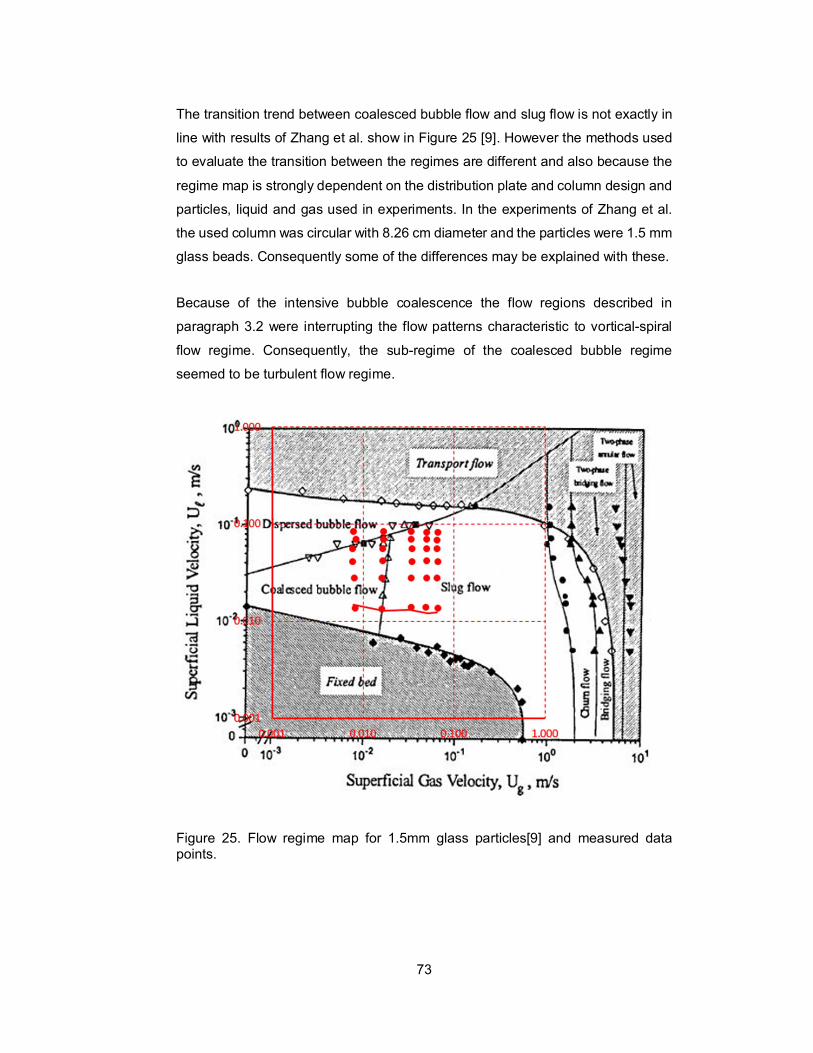
73
The transition trend between coalesced bubble flow and slug flow is not exactly in
line with results of Zhang et al. show in Figure 25 [9]. However the methods used
to evaluate the transition between the regimes are different and also because the
regime map is strongly dependent on the distribution plate and column design and
particles, liquid and gas used in experiments. In the experiments of Zhang et al.
the used column was circular with 8.26 cm diameter and the particles were 1.5 mm
glass beads. Consequently some of the differences may be explained with these.
Because of the intensive bubble coalescence the flow regions described in
paragraph 3.2 were interrupting the flow patterns characteristic to vortical-spiral
flow regime. Consequently, the sub-regime of the coalesced bubble regime
seemed to be turbulent flow regime.
Figure 25. Flow regime map for 1.5mm glass particles[9] and measured datapoints.
74
The particle movement velocities appear to be more dependent on the liquid flow
velocity than on the gas flow velocity. Whereas the bubbles seems to cause more
disordered movement which results in stronger mixing of the particles. This
phenomenon resembles strongly the wake model: bubbles moving up form a wake
behind the bubble. Particles in the bed are sucked into the wake and moved
upwards behind the bubble. And when a bubble reaches the surface of the bed
some particles are thrown into freeboard region.
From the experiments it is also observed that the bubble distribution in the column
is depending on the superficial gas flow velocity. With lower gas velocities the
bubbles are distributed more evenly along the whole bed so that the bubbles are
observed also near the column walls. However, with higher gas velocities the
bubbles are not observed in the vicinity of the wall as frequently as with lower gas
velocities indicating that bubbles tends to concentrate more on central parts of the
column with the increase of gas flow velocity. In addition, regardless of the flow
velocities the bubbles tend to be more visible near the distribution plate. And when
going further away from the plate the amount of bubbles appearing in the vicinity
of the walls decreases.
12 Recommendations for improvements and future work
Here are some possible improvements that were discovered during the
experiments. Some of these improvements are general and some only for the
column used in these experiments.
12.1 Particles motion detection and tracking
With experiment setting like the one used in this thesis it would be rather easy to
follow and obtain the movement data of the colored tracer particles. Because
usually the flow pattern in the column is not symmetrical so for comprehensive data
from the vicinity of the wall it is necessary to recording all sides of the column.
However with video recording methods the particle movement deeper in the bed
is, especially with air-water-glass combination, still almost impossible to see.
75
For analyzing the recordings and to obtain movement data motion detection
software is needed. It is possible to build particle tracking program for example with
help of OpenCV library. For accurate movement detection and particle tracking it
is crucial to have video with high frame rate and high resolution.
12.2 Refractive index matching
For future experiments refractive index matching technics would be worth looking
into especially if the future experiments are concerning the particle movement.
With air-water-glass bead –system the particles are only able to be observed closer
than approximately one centimeter away from the column walls. Choices for
refractive index matching are to change the particles to match the liquid or to
change or alter the liquid to match the refractive index of the particles.
12.3 Observing all sides of the column
The particles movement were recorded only on one side of the rectangular column.
However it was clear when visually observed that the flow patterns are dissimilar
in other sides of the column. For more accurate analysis it would be necessary to
record all sides simultaneously. This could be possible for example setting mirrors
so that one camera can record all sides simultaneously or just simply by recording
with multiple cameras.
12.4 Paint for tracking particles
In the experiments done for this thesis the tracer particles were marked just by
painting them with general spray-paint. However the particles in the bed are
undergoing rather severe conditions so that the paint in the particles is gradually
peeling off during the experiments. For future experiments it would be worth looking
into what kind of paint would be more resistant for wearing.
12.5 Defining the height of the bed
One of the factors generating inaccuracy to the bed expansion measurements was
the difficulty in defining the exact bed height of the fluidized bed. The visual
observation for accurate measurements was noticed to be inadequate method
since especially with higher superficial gas flow velocities the particle entrainment
76
to the freeboard region is so substantial that the bed level appears to be varying
all the time.
Because the axial dynamic pressure distribution has linear behavior in both
fluidized bed and freeboard region above the bed, the bed height can be defined
from pressure measurements. These measurements requires at least 4 pressure
sensor altogether, two in freeboard region and two within the bed. The point where
these pressure profiles intersect is the point where the bed level is.[1]
12.6 Bubble size measurements
With the experiment setup used, it was really difficult to assess the bubble sizes
and size distribution in the bed. So in future studies it would be worthwhile to use
tools such as conductivity probe to obtain more comprehensive data of the bubbles.
With conductivity probe it is possible to obtain data of for example bubble frequency,
bubble size, bubble velocity, bubble shape, and to use in calculating the gas hold-
up[9].
12.7 Gas and liquid valves
During the experiment there were problems with both gas and liquid valves which
regulate the flow to the column.
Problem with liquid valves was that they were causing unwanted disturbance in the
liquid flow. The problem was caused by the way valves were installed. There were
two valves connected to the hose so that the hose coming from pump was
connected to the T-fitting. Opposite side of the T-fitting was valve that regulated
the flow to the column and to the T-fitting connector not in line with others were
connected another valve that regulated the flow straight back to the liquid tank.
During the experiments it was noted that when the valve to the tank was open, this
valve setting caused severe disturbance in the flow resulting uneven flow to the
column, consequently causing considerable disturbance in the pressure
measurements.
These problems can be diverted by changing the valves for more suitable ones.
As a short term solution, the valve to the liquid tank can be closed but it increases
77
the stress to the pump especially with low superficial flow velocities in the column.
The valves used had also some controllability challenges. So by replacing the
valves by valves that are easier to control would even more advantageous.
The valve in the gas line was problematic because it was really sensitive so that
adjusting the desired flow rate was difficult. On top of that the gas flow coming from
the line was intermittent irregular which made it even more challenging to adjust
constant desired flow rate. These problems can be averted to install more sensitive
or possibly automatic valves.
12.8 Homogenize the liquid and gas flows and reducing the sizes ofbubbles entering the bed
Even if the column has 50 cm long homogenizing section the uneven velocity
distribution below the distribution plate was observed. This might be due to the
method how the liquid hose is connected to the column. Just below the column
there is T-fitting where the flowing liquid makes 90 degree turn. By altering this
connection the liquid flow might become more uniform. The calming section can
be made more effective also by filling it with packing. The packing will equalize the
flow profile prior to the bed.
Another unwanted feature of the column is the gas distribution nozzle. The bubbles
leaving the nozzle are not distributed evenly to the whole column area and the
generated bubble sizes are rather nonuniform. Desired situation would be that the
bubbles were small, uniform in size and distributed evenly along the column cross-
section. By changing the design of the nozzle it would be possible to affect the
bubbles generated and the distribution of them.
12.9 Reduce column shaking
Especially with high gas and liquid flows quite severe column shaking was
observed. This might be due to the turbulence in the column. And because the
attachment is not as sturdy as hoped causing the shaking to be more intensive
than desired. The shaking may cause some interference to the pressure
measurements which causes the interpreting of measured data slightly more
78
challenging. The shaking may be reduced by installing the column to sturdier
mount.
79
13 References
[1] Fan Liang-Shih. Gas-liquid-solid fluidization engineering. Stoneham, MA:Butterworth Publishers, 1989 ISSN/ISBN 978-0409951790.
[2] Wilhelm, Richard H. & Kwauk, Mooson. Fluidization of solid particles.Chemical Engineering Progress. 1948, vol. 44: 3.
[3] Davidson J. F., Clift R.& Harrison D. Fluidization. 2. ed. London: Academic,1985 ISSN/ISBN 0-12-205552-7.
[4] Jakobsen Hugo A. Chemical reactor modeling. Berlin: Springer, 2008ISSN/ISBN 978-3-540-68622-4.
[5] Gidaspow Dimitri. Multiphase flow and fluidization: continuum and kinetictheory descriptions. London: Academic press, 1994 ISSN/ISBN 9780122824708.
[6] Harker J. H., Backhurst J. R.& Richardson J. F. Chemical Engineering Volume2. 5. ed. Woburn, MA: Butterworth Heinemann, 2002 ISSN/ISBN 978-0-7506-4445-7.
[7] Kunii Daizo& Levenspiel Octave. Fluidization engineering. 2. ed. Stoneham,MA: Butterworth-Heinemann, 1991 ISSN/ISBN 9780409902334.
[8] Muroyama, Katsuhiko & Fan, Liang-Shih. Fundamentals of gas-liquid-solidfluidization. AIChE Journal. 1985, vol. 31: 1.
[9] Zhang, J-P, Grace, JR, Epstein, N. & Lim, KS. Flow regime identification ingas-liquid flow and three-phase fluidized beds. Chemical Engineering Science.1997, vol. 52: 21.
[10] Chen, RC, Reese, J. & Fan, L-S. Flow structure in a three-dimensional bubblecolumn and three-phase fluidized bed. AIChE Journal. 1994, vol. 40: 7.
[11] Fan, Liang Shih, Chern, SH & Muroyama, K. Solids mixing in a gas liquidsolid fluidized bed containing a binary mixture of particles. AIChE Journal. 1984,vol. 30: 5.
[12] Larachi, F., Cassanello, M., Chaouki, J. & Guy, C. Flow structure of the solidsin a 3 D gas–liquid–solid fluidized bed. AIChE Journal. 1996, vol. 42: 9.
[13] Tzeng, J W, Chen, RC & Fan, L S. Visualization of flow characteristics ina 2 D bubble column and three phase fluidized bed. AIChE Journal. 1993, vol.39: 5.
[14] Stewart, P. S. B. & Davidson, J. F. Three-phase fluidization: Water, particlesand air. Chemical Engineering Science. 1964, vol. 19: 4. ISSN 0009-2509.
80
[15] Matsuura, Akinori & Fan, Liang-Shih. Distribution of bubble properties in agas-liquid-solid fluidized bed. AIChE Journal. 1984, vol. 30: 6. ISSN 1547-5905.
[16] Zenz Frederick A.& Othmer Donald F. Fluidization and fluid-particle systems.New York: Reinhold publishing corporation, 1960
[17] Peterson, D. A., Tankin, R. S. & Bankoff, S. G. Bubble behavior in a three-phase fluidized bed. International Journal of Multiphase Flow. 1987, vol. 13: 4.ISSN 0301-9322.
[18] Leva Max, Weintraub Murray, Grummer Milton, Pollchik Morris& StorchHH. U.S Bureau of Mines, Bulletin 504: Fluid flow through packed and fluidizedsystems. Washington: US Government Printing Office, 1951
[19] Solimene, R., Aprea, G., Chirone, R., Marzocchella, A. & Salatino, P.Hydrodynamic Characterization of" GULF STREAM" Circulation in a Pilot ScaleFluidized Bed Combustor. 2013
[20] McKetta John J. Encyclopedia of Chemical Processing and Design: Volume23 - Fluid Flow. New York: Marcel Dekker Inc., 1985 ISSN/ISBN 0824724739.
[21] Cassanello, Miryan, Larachi, Faïçal, Guy, Christophe & Chaouki, Jamal.Solids mixing in gas-liquid-solid fluidized beds: Experiments and modelling.Chemical Engineering Science. 1996, vol. 51: 10. ISSN 0009-2509.
[22] Cassanello, Miryan, Larachi, Faiecal, Marie, Marie-Noelle, Guy, Christophe& Chaouki, Jamal. Experimental characterization of the solid phase chaoticdynamics in three-phase fluidization. Industrial & Engineering ChemistryResearch. 1995, vol. 34: 9.
[23] Mostoufi, N. & Chaouki, J. Prediction of effective drag coefficient in fluidizedbeds. Chemical Engineering Science. 1999, vol. 54: 7.
[24] Grbavčić, Željko B., Vuković, DV, Jovanović, SDJ & Littman, H. The effectivebuoyancy and drag on spheres in a water-fluidized bed. Chemical engineeringscience. 1992, vol. 47: 8.
[25] Wen, C. & Yu, YH. Mechanics of fluidization. Chemical engineering progresssymposium series. 1966, vol. 62: 62.
[26] Gupta Chiranjib K.& Sathiyamoorthy D. Fluid bed technology in materialsprocessing. Boca Raton, Florida: CRC Press, 1998 ISSN/ISBN 0-8493-4832-3.
[27] Larachi, Faïçal, Belfares, Lamia, Iliuta, Ion & Grandjean, Bernard PA. Three-phase fluidization macroscopic hydrodynamics revisited. Industrial & EngineeringChemistry Research. 2001, vol. 40: 3.

81
[28] Ergun, Sabri. Fluid flow through packed columns. Chemical engineeringprogress. 1952, vol. 48
[29] Østergaard, K. & Theisen, PI. The effect of particle size and bed height on theexpansion of mixed phase (gas—liquid) fluidized beds. Chemical EngineeringScience. 1966, vol. 21: 5.
[30] Rigby, GR & Capes, CE. Bed expansion and bubble wakes in three phasefluidization. The Canadian Journal of Chemical Engineering. 1970, vol. 48: 4.
[31] Richardson, JF & Zaki, WN. Sedimentation and fluidisation: Part I.Transactions of the Institution of Chemical Engineers. 1954, vol. 32
[32] Akgiray, Omer & Soyer, Elif. An evaluation of expansion equations forfluidized solid-liquid systems. Aqua- Journal of Water Supply: Research andTechnology. 2006, vol. 55: 7.
[33] Shi, Yan-Fu & Fan, L. T. Effect of distributor to bed resistance ratio onuniformity of fluidization. AIChE Journal. 1984, vol. 30: 5. ISSN 1547-5905.
[34] Siegel, Robert. Effect of distributor plate to bed resistance ratio on onset offluidized bed channeling. AIChE Journal. 1976, vol. 22: 3.
[35] Foscolo, PU & Gibilaro, LG. A fully predictive criterion for the transitionbetween particulate and aggregate fluidization. Chemical Engineering Science.1984, vol. 39: 12.
[36] Kwauk, Mooson, Li, Jinghai & Liu, Dejin. Particulate and aggregativefluidization—50 years in retrospect. Powder Technology. 2000, vol. 111: 1.
[37] Liu, Dejin, Kwauk, Mooson & Li, Hongzhong. Aggregative and particulatefluidization—the two extremes of a continuous spectrum. Chemical EngineeringScience. 1996, vol. 51: 17.
[38] Wen, CY & Yu, YH. A generalized method for predicting the minimumfluidization velocity. AIChE Journal. 1966, vol. 12: 3.
[39] Epstein, Norman. Applications of liquid-solid fluidization. InternationalJournal of Chemical Reactor Engineering. 2003, vol. 1: 1.
[40] Shen, Laihong, Zhang, Mingyao & Xu, Yiqian. Solids mixing in fluidized beds.Powder Technology. 1995, vol. 84: 3.
[41] Zhang, Yong, Zhong, Wenqi & Jin, Baosheng. New method for theinvestigation of particle mixing dynamic in a spout-fluid bed. Powder Technology.2011, vol. 208: 3.

82
[42] Westphalen, Detlef & Glicksman, Leon. Lateral solid mixing measurements incirculating fluidized beds. Powder Technology. 1995, vol. 82: 2.
[43] Zhang, Yong, Jin, Baosheng & Zhong, Wenqi. Experiment on particle mixingin flat-bottom spout–fluid bed. Chemical Engineering and Processing: ProcessIntensification. 2009, vol. 48: 1.
[44] Lacey, P. M. C. Developments in the theory of particle mixing. Journal ofapplied chemistry. 1954, vol. 4: 5.
[45] Boyer, Christophe, Duquenne, Anne-Marie & Wild, Gabriel. Measuringtechniques in gas–liquid and gas–liquid–solid reactors. Chemical EngineeringScience. 2002, vol. 57: 16.
[46] Werther, Joachim. Measurement techniques in fluidized beds. PowderTechnology. 1999, vol. 102: 1. ISSN 0032-5910.
[47] Chaouki, Jamal, Larachi, Faical & Dudukovic, Milorad P. Noninvasivetomographic and velocimetric monitoring of multiphase flows. Industrial &Engineering Chemistry Research. 1997, vol. 36: 11.
[48] Budwig, R. Refractive index matching methods for liquid flow investigations.Experiments in Fluids. 1994, vol. 17: 5.
[49] Larachi, Faïçal, Kennedy, Gregory & Chaouki, Jamal. A γ-ray detection systemfor 3-D particle tracking in multiphase reactors. Nuclear Instruments and Methodsin Physics Research Section A: Accelerators, Spectrometers, Detectors andAssociated Equipment. 1994, vol. 338: 2.
[50] Handley, D., Doraisam, A., Butcher, KL & Franklin, NL. A study of fluid andparticle mechanics in liquid-fluidised beds. transactions of the institution ofchemical engineers. 1966, vol. 44: 7.
[51] Prasad, Ajay K. Particle image velocimetry. Current Science. 2000, vol. 79: 1.
[52] Raffel Markus, Willert Christian E., Wereley Steve T.& Kompenhans Jürgen.Particle image velocimetry : a practical guide. 2. ed. Berlin: Springer, 2007ISSN/ISBN 978-3-540-72307-3.
[53] Shirsath, SS, Padding, JT, Clercx, HJH & Kuipers, JAM. Cross-validation of3D particle tracking velocimetry for the study of granular flows down rotatingchutes. Chemical Engineering Science. 2015
[54] Buist, Kay A., Gaag, Alex C., Deen, Niels G. & Kuipers, Johannes AM.Improved magnetic particle tracking technique in dense gas fluidized beds. AIChEJournal. 2014, vol. 60: 9.
83
[55] Avidan, Amos & Yerushalmi, Joseph. Solids mixing in an expanded top fluidbed. AIChE Journal. 1985, vol. 31: 5.
[56] Valenzuela, JA & Glicksman, LR. An experimental study of solids mixing in afreely bubbling two-dimensional fluidized bed. Powder Technology. 1984, vol. 38:1.
[57] Glicksman, Leon, Carr, Ezra & Noymer, Peter. Particle injection and mixingexperiments in a one-quarter scale model bubbling fluidized bed. PowderTechnology. 2008, vol. 180: 3.


![Comparisons of particle cluster diameter and concentration in … · 2013. 3. 26. · particle cluster prohibits a good multiphase mixing inside the sys-tem [4]. This then has negative](https://img.dokumen.tips/doc/110x75/5fe50b0de43dd3796b250bc4/comparisons-of-particle-cluster-diameter-and-concentration-in-2013-3-26-particle.jpg)