IMPERIAL COLLEGE LONDON

Faculty of Engineering

Department of Civil and Environmental Engineering

Structural Controls on the

Hydrogeology of Malta

Christian Schembri

September 2014

Submitted in fulfilment of the requirements for the MSc and the Diploma of Imperial College London

Page | ii

DECLARATION OF OWN WORK

Declaration:

This submission is my own work. Any quotation from, or description of, the

work of others is acknowledged herein by reference to the sources, whether

published or unpublished.

Signature : ___________________________________

Page | iii

To my beloved wife Rosanne

Page | iv

The research work disclosed in this publication is partially funded by the Master it!

Scholarship Scheme (Malta). This Scholarship is part-financed by the European

Union – European Social Fund (ESF) under Operational Programme II – Cohesion

Policy 2007-2013, “Empowering People for More Jobs and a Better Quality Of Life.

Operational Programme II – Cohesion Policy 2007-2013

Empowering People for More Jobs and a Better Quality of

Life

Scholarship part-financed by the European Union

European Social Fund (ESF)

Co-financing rate: 85% EU Funds;15% National Funds

Investing in your future

Page | v

Acknowledgements

First and foremost I would like to thank my wife Rosanne for her emotional support

over the last year. The past year has been a challenge for both of us and thus I

would also like to thank our extended family members and friends for their support.

Special thanks go to Dr Clark Fenton of the Imperial College London for his help,

inspiration and guidance over the last year and to the staff at the Geotechnics

Department.

I would also like to thank Dr Martyn Pedley and Dr Adrian Butler for their replies for

my queries. I would like to express my gratitude to Adrian Mifsud for his assistance

during my field trip and interest. Thanks go also to Solidbase Laboratories Ltd and

Joe Bugeja for allowing me access to certain documents.

Thanks go to Roderick Vella from the Transport and Infrastructure Ministry of Malta

for providing me with useful contacts during data collection and Manuel Sapiano for

providing me with access to past reports and for his prompt replies to my queries.

My gratitude goes also to my fellow students who have been ideal colleagues and

friends throughout the year.

Page | vi

Executive Summary

The main aim of this study is to identify and understand structural controls on the

hydrogeology of Malta.

An introduction chapter provides a general geologic context of Malta, followed by a

detailed aim and an overall view of the study. This is followed by an extensive

literature review providing a sound geologic and hydrogeologic background.

The Maltese Islands are located in the foreland of the Apennine-Maghrebian thrust

and fold belt and are affected by an extensional tectonic environment. An onshore

expressed of this are the horst and graben structures widely observable in the range

between the South of Gozo fault (or Il-Qala fault) and the Victoria fault. Tectonics

controlled the sedimentation processes. Similar processes but more pronounced

were taking place at the offshore regional grabens of the Pantelleria rift and the

North Gozo graben. Higher extensional strains are reported in the latter basins than

what is reported for onshore Malta. The uplift of the Maltese Islands occurred

during some period stretching between the late Messinian to the mid-Pliocene. The

geologic formations of Malta consist in sedimentary marine carbonates deposited at

shallow sea depths with the highest sea depths estimated not to be greater than

250 metres. These include from top, the Upper Coralline Limestone (UCL),

Greensand, Blue Clay (BC), Globigerina Limestone (GL) and Lower Coralline

Limestone (LCL).

Malta has two main types of aquifers being the perched aquifer on top of the BC

and the mean sea level aquifer which is predominantly hosted by the LCL. The

aquifers are dual-porosity as flow may take place through the rock matrix and the

fracture network. Faults may have two contrasting effects. They may provide a seal

or increase the density of the fracture network.

The main data collection process included a one-week field trip during which a

geomorphologic site reconnaissance exercise was carried out and discontinuity scan

line data was collected. Previous data was also acquired and is re-interpreted and

Page | vii

used. This data set includes investigation borehole logs, well pumping tests

determining aquifer transmissivity and potentiometric data. Previous data is

generally limited to a regional context, incomplete and does not satisfy directly the

scope of this study. Predictive data from previous field studies is used to augment

our understanding of the effects of faults on the hydraulic conductivity of rock

masses. A detailed observations and analysis chapter is presented. The main

findings are summarised as follows:

• The hypothesis that joints are closely linked to the latest rift tectonics of

Malta is presented. Evidence includes similar strikes and dip angles of the

most occurring joints that closely resemble the ENE-WSW and NW-SE

trending faults and the wider apertures of these joints.

• Exceptions to the above rule may be present as is observed at the site of

Birkirkara where the main trending joint set J8 shows strike similarity to the

ENE-WSW trending faults but occurs at a much shallower dip. This probably

is related to another structure which in literature is described as the up-

arching of the LGL prior to the rifting process.

• From observations it is noted that karst development differs between

formations or facies that exhibit variability in hydraulic permeability due to

grain size distribution and fracturing. In addition observations highlight that

fluid conducting boundaries can result between layers of different grain size

distributions.

• A plot of spatial transmissivity in relation to distance from faults, although

from low resolution and an incomplete data set, provides encouraging

indications for future research as a certain degree of correlation between

the two seems plausible.

Page | viii

Table of Contents

Acknowledgements ...................................................................................................... v

Executive Summary ..................................................................................................... vi

Table of Contents ....................................................................................................... viii

Tables ...........................................................................................................................xi

Figures ......................................................................................................................... xii

1 Introduction .......................................................................................................... 1

1.1 Scope of Work ............................................................................................... 3

1.2 Overview of Work .......................................................................................... 4

2 Geologic and Hydrogeologic Background of Malta .............................................. 6

2.1 Geologic Background ..................................................................................... 6

2.1.1. Tectonic Setting ...................................................................................... 6

2.1.2. Tectonic History Debates ..................................................................... 11

2.1.3. Onshore Structural Geology of Malta .................................................. 12

2.1.4. Main Stratigraphical Units ................................................................... 14

2.2 Hydrogeologic Background ......................................................................... 17

2.2.1. Basic Hydroclimatological data ............................................................ 17

2.2.2. Water Balance ...................................................................................... 18

2.2.3. Hydrogeological Setting ....................................................................... 18

2.2.4. Effects of faults on fluid flow ............................................................... 20

2.2.5. Aquifer hydraulic properties ................................................................ 22

2.2.6. Geochemical Studies ............................................................................ 23

3 Methods .............................................................................................................. 25

3.1 Geomorphologic Site Reconnaissance ........................................................ 26

3.2 Dip (angles) and dip directions of discontinuities ....................................... 27

3.3 Other discontinuities characteristics ........................................................... 30

3.3.1. Relative hydraulic conductivity ............................................................ 30

3.4 Transmissivity .............................................................................................. 31

3.5 Potentiometry ............................................................................................. 32

3.6 Control of fault parameters on hydraulic properties .................................. 33

3.6.1. Displacements along fault lengths ....................................................... 33

3.6.2. Length and termination points of faults .............................................. 35

Page | ix

3.6.3. Fault architecture at a cross-section .................................................... 36

3.6.4. Strata thickness and properties ........................................................... 37

4 Observations and Analysis .................................................................................. 38

4.1 Geomorphologic Site Reconnaissance ........................................................ 38

4.1.1. Qammiegh ............................................................................................ 38

4.1.2. L-Imgiebah Bay ..................................................................................... 41

4.1.3. Fomm ir-Rih Bay ................................................................................... 45

4.1.4. Wied il-Ghasel ...................................................................................... 48

4.1.5. Gharghur .............................................................................................. 48

4.1.6. St. George’s Bay ................................................................................... 51

4.1.7. Msida .................................................................................................... 52

4.1.8. Xghajra ................................................................................................. 54

4.1.9. Munxar ................................................................................................. 56

4.2 Inferring Contacts from Boreholes .............................................................. 58

4.2.1. UCL/BC ................................................................................................. 58

4.3 Dip (angles) and dip directions of discontinuities ....................................... 59

4.3.1. Fomm ir-Rih Bay ................................................................................... 59

4.3.2. St. George’s Bay ................................................................................... 60

4.3.3. Msida .................................................................................................... 61

4.3.4. Xghajra ................................................................................................. 61

4.3.5. Birkirkara .............................................................................................. 62

4.4 Other discontinuities characteristics ........................................................... 63

4.4.1. Aperture ............................................................................................... 63

4.4.2. Persistence ........................................................................................... 64

4.4.3. Relative hydraulic conductivity (K) ....................................................... 66

4.5 Transmissivity .............................................................................................. 66

4.6 Potentiometry ............................................................................................. 71

5 Discussion ........................................................................................................... 72

5.1 Geomorphologic Site Reconnaissance ........................................................ 72

5.1.1. Stratal Dip of BC ................................................................................... 72

5.1.2. Flow indications from karst erosion ..................................................... 73

5.1.3. Sedimentation processes ..................................................................... 74

5.1.4. Calcite Deposition ................................................................................ 74

Page | x

5.1.5. Style of faulting .................................................................................... 75

5.2 Discontinuity data ....................................................................................... 75

5.2.1. Jointing link with the rifting tectonics of Malta ................................... 75

5.2.2. Limited data from persistence ............................................................. 76

5.2.3. The case of the Birkirkara site .............................................................. 76

5.2.4. Extent of tectonic affect ....................................................................... 77

5.2.5. Control on hydraulic conductivities from geologic contacts ............... 77

5.2.6. Jointing link with nearest fault structure ............................................. 78

5.2.7. Further data limitations ....................................................................... 78

5.3 Transmissivity .............................................................................................. 79

5.4 Potentiometry ............................................................................................. 80

5.5 Main Data Limitations ................................................................................. 80

5.6 Conceptual Ground Model .......................................................................... 81

6 Summary and Conclusions .................................................................................. 84

6.1 Main Conclusions ........................................................................................ 84

6.2 Further Studies ............................................................................................ 85

6.2.1. Fault parameters and control .............................................................. 85

6.2.2. Controls on jointing .............................................................................. 86

6.2.3. Permeability variability of different formations and facies ................. 86

6.2.4. Geochemistry ....................................................................................... 86

References .................................................................................................................. 87

Appendix A – The Geological Map of Malta (1993) ................................................... 93

Appendix B – Main water bodies as indicated by the Malta Resources Authority

(MRA) ......................................................................................................................... 95

Appendix C – Mdina investigation boreholes from Gianfranco et al. (2003) .......... 105

Appendix D – Stereonet plots .................................................................................. 116

Appendix E – Full scan lines sheets .......................................................................... 126

Appendix F – Tables and graphics of discontinuities aperture data ........................ 145

Appendix G – Tables and graphs of discontinuities persistence data ..................... 162

Appendix H – Relative hydraulic conductivities ....................................................... 172

Appendix I – Hydrodynamic data ............................................................................. 174

Appendix J – Fault data and structural contours of LCL .......................................... 179

Page | xi

Tables

Table 1 – Summary of the stratigraphical units of Malta (adopted from Pedley et al.,

1976; the Geological Map of Malta, 1993) ................................................................ 16

Table 2 – Climate parameters monthly means (source: Sapiano et al., 2006) .......... 17

Table 3 – Water balances for individual ground water bodies for the year 2003

(source: Sapiano et al., 2003). The groundwater body codes refer to groundwater

bodies as identified by the Malta Resources Authority, maps of which are presented

in Appendix B. ............................................................................................................ 18

Table 4 – Average aquifer hydraulic properties compiled from literature ................ 23

Table 5 – Table showing site names of sites included in study ................................. 26

Table 6 – Summary of discontinuity data collected. Site reference numbers are

cross-referenced to Figure 11 and Table 5. Initials CS refer to Christian Schembri and

AM refer to Geotechnical Engineer Adrian Mifsud. .................................................. 27

Table 7 – Summary of the main identifiable joint sets from pole concentrations for

each site and scan line. Site reference numbers are cross-referenced to Figure 11

and Table 5. ................................................................................................................ 28

Table 8 – Summary of the main joint sets variability of averages ............................. 29

Table 9 – Aperture ranges for each aperture width class. These aperture width

classes are used in the presentation of Appendices F and G graphs. These are the

basis for the analysis presented in Chapter 4. ........................................................... 30

Table 10 – Persistence ranges for each persistence class. These persistence classes

are used in the presentation of Appendices F and G graphs. These are the basis for

the analysis presented in Chapter 4. ......................................................................... 30

Table 11 – D and L co-ordinates used to determine a relationship in the form D=cL2

.................................................................................................................................... 34

Table 12 – Expected maximum widths for a 36m displacement using predictive

equations from Michie et al. (2014) .......................................................................... 37

Page | xii

Figures

Figure 1 – Location of the Maltese Islands is shown by the red circle (source: Google

Earth, 2014) .................................................................................................................. 1

Figure 2 – Part of the North West coast of Malta as seen from “Fomm ir-Rih” Bay ... 2

Figure 3 – Tectonic sketch of the Central Mediterranean. Approximate position of

Malta shown by the red circle. (source: Anzidei et al., 2001). Key details:

“(1)Continental (a) and oceanic (b) parts of the Africa/Adriatic and Eurasian

forelands; (2) Tethyan belt comprised of oceanic remnants and intermediate

massifs (Pelagonian, Anatolian and Cyclades arcs); (3) deformation belts developed

on the African and Eurasian margins; (4) crustal thinning; (5) active thrust fronts; (6)

subduction zones; (7) inactive thrust fronts; (8,9,10) compressional, tensional and

transcurrent feautrues; (11) main trends of compressional deformation in the

Mediterranean Ridge and Calabrian Arc.” (Anzidei et al., 2001) ................................. 6

Figure 4 – Isopach map of the LGL (source: Pedley et al., 1976) ................................. 7

Figure 5 – Focal mechanisms with principal stress directions for various major fault

zone outcrops (source: Dart et al., 1993) .................................................................... 8

Figure 6 – Diagram showing the North-South transfer fault zone between the

Pantelleria Trough to its west and the Malta Trough (also known as the Malta

Graben) and Linosa Trough to its east. These three structures form part of the

Pantelleria Rift (source: Argnani, 1990) ....................................................................... 9

Figure 7 – Diagram showing the tectonic kinematics for the Hyblean-Malta Plate and

the Ionian Plate as proposed by Jongsma et al. (1987) (source: Jongsma et al., 1987)

.................................................................................................................................... 10

Figure 8 – Simplified structural geologic map of the Maltese Islands (source: Dart et

al., 1993) ..................................................................................................................... 13

Figure 9 – Total annual rainfall for Luqa meteorological station (source: Sapiano et

al., 2006) ..................................................................................................................... 17

Figure 10 – Conceptual model of a solution subsidence structure (Pedley,

1975b:p.542) .............................................................................................................. 20

Figure 11 – Sites visited indicated on the Geological Map of Malta (1993). Sites

marked in red include only a site reconnaissance exercise while magenta sites

include also the collection of discontinuity data. Discontinuity data for site 8 was

acquired and not carried out by myself. No site visit was paid to site 8. Site numbers

are cross-referenced to Table 5. ................................................................................ 25

Figure 12 – Stereographic projection showing the entire joint set brackets

considered for grouping of all the discontinuity data overlaid over a scatter plot of

all the pole data. The inner circle represents a dip angle of 35o; poles within it

represent discontinuities with dip angles less than 35o. J9 & J10 are introduced to

include all of the data. ............................................................................................... 29

Page | xiii

Figure 13 – Points of which the details are presented in Table 11. The red line

indicates the direction along which the length of the fault is considered (adapted

from The Geological Map of Malta, 1993) ................................................................. 34

Figure 14 – Graph showing growth path of a segmented isolated fault and the

complexity to determine this relationship due to field data scatter. For inter-linked

overlapping faults the difference between the green point and the blue point

depends on what fault length is considered. (adapted from Cartwright et al., 1995)

.................................................................................................................................... 35

Figure 15 – Cumulative heave plot for a cliff scale section named Malta D with

location shown on map. Red lines on plot indicate single faults having major heave

spaced at approximately 600 metres. (adapted from Putz-Perrier & Sanderson, 2010)

.................................................................................................................................... 37

Figure 16 – Aerial photo of Qammiegh Site (adapted from Google Earth, 2014). The

red polylines encircle slope instability areas which mainly involve rock toppling. The

blue polyline encircle a wetland and saltmarsh. Black lines show the locations of

faults and where they are dashed it means that they are inferred (The Geological

Map of Malta, 1993). Numbers are cross-referenced with photo numbers of this

section and the arrows show the orientation of view. .............................................. 38

Figure 17 – Photo 1. Arrows indicate extent of main karst features and dashed lines

show enlarged joints observed from distance. .......................................................... 39

Figure 18 – Photo 2 showing extensive cave development at Fault Zone. Dashed line

indicates inferred fault (The Geological Map of Malta, 1993). ................................. 40

Figure 19 – Photo 3 showing UCL hanging wall ......................................................... 40

Figure 20 – Photo 4 showing varying slope angles along a slope section. Red lines

indicate general slope angles of every formation. .................................................... 41

Figure 21 – Aerial photo of L-Imgiebah Bay (adapted from Google Earth, 2014). The

red polylines encircle slope instability area. The green polylines encircle denser

vegetated areas. Numbers are cross-referenced with photo numbers of this section

and the arrows show the orientation of view. .......................................................... 42

Figure 22 – Photo 1 showing cliff edge with the BC overlying the UGL. Dashed lines

indicate joints into the plane of the paper (approx. ENE-WSW), dotted polylines

indicate joints parallel to the plane of the paper (approx. NW-SE)........................... 43

Figure 23 – Photo 2 showing desiccated clay surface ............................................... 43

Figure 24 – Photo 3 showing oxidised UGL joint as interpreted by Missenard et al. (2014) ......................................................................................................................... 43

Figure 25 – Photo 4 showing UCL cliff edge exhibiting at least two dominant

discontinuity sets. For explanation of annotations used refer to Figure 22. ............ 44

Figure 26 – Aerial photo of Fomm ir-Rih Bay (adapted from Google Earth, 2014).

Numbers are cross-referenced with photo numbers of this section and the arrows

show the orientation of view. .................................................................................... 45

Page | xiv

Figure 27 – Photo 1 showing Victoria fault at west coast outcrop. Annotations used

are explained by notes on photo. .............................................................................. 45

Figure 28 – Photo 2 showing detail of antithetic fault shown in Figure 27. ............. 47

Figure 29 – Photo 3 showing LGL outcrop at location of Scan line A (scale shown by geologic hammer) .................................................................................................. 47

Figure 30 – Photo 4 shows MGL at location of scan line B. Dashed lines show

examples of sub-horizontal desiccation joints (scale shown by field notebook) ...... 47

Figure 31 – Photo 5 showing the Lower Main Phosphorite Conglomerate (scale

shown by field notebook scale line) .......................................................................... 47

Figure 32 – Karst caves in the Attard member of the LCL at Wied il-Ghasel where it

cross-cuts the Victoria fault, the rock face strike is approximately NNE ................... 48

Figure 33 – Aerial photo of site visited at Gharghur (adapted from Google Earth,

2014). The green line shows a stretch of denser vegetation. Numbers are cross-

referenced with photo numbers of this section and the arrows show the orientation

of view. ....................................................................................................................... 49

Figure 34 – Photo 1 showing formed notches at Xlendi member of the LCL. Dashed

polyline indicates a wider aperture joint. .................................................................. 50

Figure 35 – Photo 2 showing detail of calcite deposition .......................................... 50

Figure 36 – Photo 3 showing karstified cave pillar .................................................... 50

Figure 37 – Infilled joint having wide aperture .......................................................... 51

Figure 38 – Fault Breccia ............................................................................................ 51

Figure 39 – Wide open aperture at fault zone ........................................................... 51

Figure 40 – Schematic plan layout of Excavation site visited at Msida with an

indication of the excavation faces references .......................................................... 53

Figure 41 – Minor Karst feature noted at wall A ....................................................... 53

Figure 42 – Excavation face A with dotted lines indicating discontinuity zones (scale

is shown by excavator) ............................................................................................... 53

Figure 43 – Excavation face B with dotted lines indicating discontinuity zones (scale

is shown by excavator) ............................................................................................... 54

Figure 44 – Excavation face D on the left side, face B on the right side and face C in

between. Discontinuity zones are indicated by dotted lines (scale is shown by

excavator) ................................................................................................................... 54

Figure 45 – Aerial photo of site visited at Xghajra (adapted from Google Earth, 2014).

Dashed lines show examples of NE discontinuities which can be observed even from

this aerial photo. ........................................................................................................ 55

Figure 46 – Photo 1 showing NE trending discontinuities on the LGL wall and on the

LCL ground (scale shown by field notebook. Dashed lines show discontinuity dip

angles. The polyline shows a karstified stretch on the LCL ground. .......................... 56

Page | xv

Figure 47 – Photo 2 showing contact between LGL and LCL and Scutella echinoids

marker (scale shown by field notebook).................................................................... 56

Figure 48 – Aerial photo of Munxar Site (adapted from Google Earth, 2014) .......... 57

Figure 49 – Photo 2. Dashed lines show examples of tight discontinuities which may

be interpreted as sedimentation desiccation discontinuities. (scale shown by field

notebook scale line) ................................................................................................... 57

Figure 50 – Photo 1 showing a low MGL cliff face ..................................................... 58

Figure 51 – Investigation boreholes location encircled in red (source: Google Earth,

2014) .......................................................................................................................... 58

Figure 52 – MGL outcrop at Fomm ir-Rih Bay scan line B. Dashed lines show main

joints. .......................................................................................................................... 60

Figure 53 – Cave-like structure adjacent to the position of the start of scan line A . 62

Figure 54 – Photo of Birkirkara site showing undulating discontinuity (scale shown

by mobile crane) ........................................................................................................ 63

Figure 55 – Variability of transmissivity with borehole depth below top of LCL (line

shown is the trend line) ............................................................................................. 67

Figure 56 – Variability of transmissivity with borehole depth with respect to the

mean sea level (line shown is the trend line) ............................................................ 68

Figure 57 – Variability of transmissivity in relation to distance away from fault

considered at surface. Black line shows a possible trend line if data points above the

red arrow and in the circle are ignored. .................................................................... 69

Figure 58 – Variability of transmissivity in relation to distance away from fault

considered at depth of borehole end. Black line shows a possible trend line if data

points above the red arrow and in the circle are ignored. ........................................ 69

Figure 59 – 1990 potentiometric map superimposed on the Geological Map of Malta

(1993). Dashed lines show main faults average alignments, dots with number show

locations of gauged boreholes with water piezometric level. (adapted from BRGM,

1991c & the Geological Map of Malta, 1993) ............................................................ 71

Figure 60 – The Victoria fault within the regional geology (adapted from the

Geological Map of Malta, 1993)................................................................................. 78

Figure 61 – Red border shows the area of the conceptual ground model presented

in this section (adapted from the Geological Map of Malta, 1993) .......................... 81

Figure 62 – Conceptual Ground Model highlighting regional hydrogeology of Malta. Annotations cross-referenced to numbers are included on the next page. ................ 82

Page | 1

1 Introduction

The Maltese Islands are located in the Mediterranean Sea, about 90km south of

Sicily and about 300km east of Tunisia. The location of the Maltese archipelago is

shown (Figure 1).

Figure 1 – Location of the Maltese Islands is shown by the red circle (source: Google Earth, 2014)

The geologic strata consist in marine sedimentary and are predominantly made up

of carbonates. Five main stratigraphic units are identified with the oldest being the

Lower Coralline Limestone (LCL) of Chattian age from the Oligocene and the

youngest the Upper Coralline Limestone (UCL) from the early Messinian period of

the Miocene. The Coralline Limestones usually form bare karstic plateaux in the

landscape while the Globigerina Limestone (GL) produces gentler landscape (Pedley

et al., 1976). In exposed Blue Clay (BC) slopes, drainage gullies and rock toppling of

the overlying UCL can be observed especially along the North West coast of Malta

(Devoto et al., 2012; Figure 2). The BC is the most fertile unit (Pedley et al., 1976)

owing in part to its low permeability characteristics. The soil produced from the

water solution of the Upper Coralline Limestones tends to be fertile too (BRGM,

250km

Page | 2

1991) and that explains the fact that a good number of solution subsidence

structures are occupied by agricultural fields.

Figure 2 – Part of the North West coast of Malta as seen from “Fomm ir-Rih” Bay

North of the Victoria Fault, Malta is dominated by horst and graben structures. Two

main fault sets outcrop on Malta with one trending approximately ENE-WSW and

the other NW-SE.

Malta has two main aquifer types. The upper perched aquifer overlying the BC

formation which acts as an aquitard and the lower being the mean sea level aquifer

of the Ghyben-Herzberg Lens type (Alexander, 1988; ATIGA, 1972; BRGM, 1991c;

Sapiano et al., 2006; Stuart et al., 2010). The BC formation can be subject to some

seepage losses which provide for some degree of connectivity between the two

aquifers. The upper perched aquifer is discontinuous and is made from several

blocks (Appendix B).

In several parts of the literature it is highlighted that the aquifers are dual porosity

with the primary porosity referring to the matrix permeability while the secondary

refers to the permeability due to the fractures which may be altered by karstic

carbonate dissolution (Newbery, 1968; BRGM, 1991; Sapiano et al., 2006;

Bakalowicz & Mangion, 2003; Stuart et al., 2010).

60m

Page | 3

This dissertation has the aim of developing a good understanding of structural

controls on the hydrogeology of Malta as the main island of the Maltese Islands.

1.1 Scope of Work

The importance of water to support life is undebatable. During the last decades

Malta has witnessed increasing demand for water resources while water recharge

remained low. The unbalance between water demand and supply has sometimes

resulted in diminishing water quality. It is therefore to no one’s surprise that

hydrogeologic studies of Malta generally deal with the hydrologic balance, water

quality and water management strategies (ATIGA, 1972; BRGM, 1991; Sapiano et al.,

2006; Stuart et al., 2010). The study of structural controls on the hydrogeology of

Malta has therefore been a neglected subject. However a new interest from the

petroleum industry to characterise the hydraulic properties of Malta’s geology

seems to be on the rise. Missenard et al. (2014) describe Malta as an open

laboratory of the Mediterranean which can possibly provide hints for offshore

explorations in the Mediterranean region.

Detailed studies from the petroleum industry even though their interest is not

geared towards understanding the hydrogeology may provide good data that can

be used to better understand the hydrogeology. In order to better understand the

structural controls on the hydrogeology of Malta an extensive literature review and

desk study coupled by a limited amount of field work are carried out. This scope

includes:

• the identification of main controls from geomorphologic site reconnaissance,

• a study of scan line discontinuity data carried out at random sites with an

analysis of the main parameters, how these relate to the regional geologic

environment is speculated and an indication of the variation of relative

hydraulic conductivity is given,

Page | 4

• re-interpretation of some spatial hydrodynamic and potentiometric data,

and

• an interpretation of the main fault controls on the hydrogeology of Malta by

combining field data with previous studies presented in a regional

conceptual ground model.

1.2 Overview of Work

The first chapter of this work gives a general background to the geology of Malta,

outlines the main aim and gives an overall overview of the work.

The second chapter presents a literature review giving a sound geologic and

hydrogeologic background of Malta. The geologic background includes tectonic

setting, tectonic history, structural geology, sedimentation environment and a brief

description of the main geologic strata. The hydrogeologic background includes

some basic hydroclimatological and water balance data, hydrogeologic setting

including the main aquifer types and some geomorphologic features realted to

hydrogeology, basic hydrogeologic characteristics of the different geologic materials,

basic hydraulic aquifer data, some observations from fault effect and from

geochemical studies.

The third chapter explains the main techniques used for data collection and its

analysis. It highlights how the methods are applied, developed and what their

limitations may be. This chapter also includes explanation of how data is going to be

presented in chapter 4. The development of a method to create a framework to

predict fracture layouts along the Victoria fault is attempted. This part of the

process serves to highlight the complexity involved and to highlight data gaps,

rather than serving the purpose of successfully providing a detailed method that

can be applied to predict fracture layouts. This part is still deemed to be very useful

in understanding the realm of structural control on the hydrogeology of Malta

especially in the piecing together of a regional conceptual ground model.

Page | 5

The fourth chapter presents observations and the analysis carried out. The topics

include geomorphologic site reconnaissance, analysis of spatial discontinuity data, a

spatial analysis of transmissivity and a small note on the potentiometric data

available. During the course of this chapter observations from one site may cross-

reference observations from another site or from literature. In so doing the pace is

set for the fifth chapter.

The fifth chapter provides the main discussion with all the observations brought

together providing a more holistic understanding of the hydrogeology of Malta. A

regional conceptual ground model is presented with this scope. The uncertainties,

data limitations, further implications and some suggestions for further studies are

included along the discussion.

The final chapter presents a summary of the main conclusions and

recommendations for further study.

Page | 6

2 Geologic and Hydrogeologic Background of Malta

2.1 Geologic Background

2.1.1. Tectonic Setting

Figure 3 – Tectonic sketch of the Central Mediterranean. Approximate position of Malta shown by the red circle. (source: Anzidei et al., 2001). Key details: “(1)Continental (a) and oceanic (b) parts of the Africa/Adriatic and Eurasian forelands; (2) Tethyan belt comprised of oceanic remnants and intermediate massifs (Pelagonian, Anatolian and Cyclades arcs); (3) deformation belts developed on the African and Eurasian margins; (4) crustal thinning; (5) active thrust fronts; (6) subduction zones; (7) inactive thrust fronts; (8,9,10) compressional, tensional and transcurrent feautrues; (11) main trends of compressional deformation in the Mediterranean Ridge and Calabrian Arc.” (Anzidei et al., 2001)

The Maltese Islands form part of the African continental plate where Miocene-

Quaternary extensional basins system formed to accommodate extension in the

foreland of the Apennine-Maghrebian thrust and fold belt (Dart et al., 1993; Argnani,

1990). The latter marks the collision zone between the African and Eurasian plates

to the north of the Maltese Islands. A tectonic sketch of the central Mediterranean

region is presented (Figure 3 sourced from Anzidei et al., 2001). This diagram gives a

general idea of the main geological structures of the region however the individual

details are the subject of various debates. At a micro plate scale the Maltese

500km

N

Pantelleria Rift

Page | 7

archipelago forms part of the Hyblean-Malta Plateau (marked IB on Figure 3; Pedley

et al., 1976).

An isopach map of the Lower Globigerina Limestone (LGL) is shown in Figure 4

(Pedley et al., 1976). This map shows thicker sections of the LGL member, which is

Aquitanian in age, close to the centre of Malta. This occurrence can be attributed to

up-arching of this member (Pedley, 1987) due to a compression action preceding

the rifting with the latter event estimated to start at approximately 21 million years

ago (Dart et al., 1993). Although this statement is plausible one would desire more

evidence to support it, however it is felt that this is outside the scope of the present

study.

Figure 4 – Isopach map of the LGL (source: Pedley et al., 1976)

A detailed study including both onshore and offshore data proposes a tectonic

hypothesis involving a north-south rift direction as responsible for the two main

fault sets found on the Maltese Islands (Dart et al., 1993). Each fault set is made up

Page | 8

of two fault sub-sets, each with the same approximate strike but with opposite dip

direction forming bounding edges of basins. They argue that there are two possible

scenarios where a single direction of stress can be responsible for this occurrence. It

can be either the re-activation of pre-existing discontinuities or a state of tri-axial

strain with the minor strain not equal to zero. In support of this hypothesis they

collect discontinuity scan line data including also slip characteristics at major fault

zones. They followed the kinematical methods proposed by Marrett & Allmendinger

(1990) and obtained focal mechanisms with the extensional stress direction being

approximately North-South for all fault exposures (Figure 5 sourced from Dart et al.,

1993).

Figure 5 – Focal mechanisms with principal stress directions for various major fault zone outcrops (source: Dart et al., 1993)

This interpretation conforms to the hypothesis of Argnani (1990), who suggests a

North-South transfer fault zone located within the Pantelleria Rift (Figure 6 sourced

from Argnani, 1990). This transfer zone accommodates differential North-South

extension and its interpretation is supported by the occurrence of strike-slip

indications along it, such as volcanic centres and a positive flower structure at the

north limb of the Pantelleria Rift. However their interpretation may contrast with

interpretations by other authors for other structures in the region.

Page | 9

Figure 6 – Diagram showing the North-South transfer fault zone between the Pantelleria Trough to its west and the Malta Trough (also known as the Malta Graben) and Linosa Trough to its east. These three structures form part of the Pantelleria Rift (source: Argnani, 1990)

Another interpretation for the kinematics of the area is given by Jongsma et al.

(1987). The authors attribute the opening of the Pantelleria Rift (also known as the

Medina Wrench zone) as a pull-apart basin due to dextral strike-slip movements.

This structure accommodates the faster movement of the Hyblean-Malta Plate and

the Ionian Plate towards the east when compared to the African and Eurasian Plates.

A component of anti-clockwise rotation about poles in the South of Italy is also

reported (Figure 7 sourced from Jongsma et al., 1987).

Grasso & Reuther (1988) as cited by Dart et al. (1993) propose that the Pantelleria

Rift formed as a pull-apart basin to accommodate strike-slip motion along the NNE-

SSW trending Scicli fault to the North of Malta and towards the South East corner of

Sicily.

Page | 10

Figure 7 – Diagram showing the tectonic kinematics for the Hyblean-Malta Plate and the Ionian Plate as proposed by Jongsma et al. (1987) (source: Jongsma et al., 1987)

The latter two hypotheses are not supported by much geomorphologic expression

neither in the Maltese Islands nor within the Pantelleria Rift (Dart et al., 1993;

Argnani, 1990). Minor exposures of strike-slip motion are witnessed in Gozo

including small scale strike-slip damage zones from the north west of Gozo (Kim et

al., 2003) and strike-slip horsetail faulting near Qala with displacements less than 1

centimetre (Illies, 1981; Pedley et al., 1976). Some features such as solution

subsidence structures near Dwejra in Gozo were interpreted as strike-slip

manifestations (Illies, 1981). A contrasting interpretation is that these faults were

formed as a cause of two solution subsidence structures in the area (Pedley, 1975b).

From extensive field studies the faults trending approximately WNW-ESE are

Page | 11

deduced to be predominantly normal dip-slip faults (Putz-Perrier, 2008; Putz-Perrier

& Sanderson, 2010; Michie et al., 2014).

Gardiner et al. (1995) reports Upper Pliocene right-lateral transtension at the North

of Gozo graben with right-stepping ridges. This activity probably reactivated the

older normal fault sets. The tectonic structural block model proposed for the

Hyblean-Malta plateau by Gardiner et al. (1995) could well combine both the

interpretations of Dart et al. (1993) and Jongsma et al. (1987) with possibly having a

rotation of the extensional axis from north-south towards north east-south west in

the last 5 million years with minimal evidence on the Maltese Islands.

The uplift of the Maltese Islands occurred from the late Messinian to the mid-

Pliocene. It is believed to be linked with the reactivation of the ENE-WSW faults by

right-lateral wrenching coupled with sea lowering during the Messinian (Pedley,

1987; Pedley, 2011). The stratigraphic units of Malta have a sub-horizontal bedding

dip towards the north-east in various areas (Pedley et al., 1976; Pedley, 1987; Dart

et al., 1993). This can also be indicative of a rising of the west coast of Malta and a

drowning of the east coast. This is strengthened by an observation of stalagmites at

the sea bottom noted during construction of the Valletta breakwater by Rizzo (1932)

as cited by Trechmann (1938). Stalagmites do not form under water.

2.1.2. Tectonic History Debates

There are a number of historical interpretations of how the two fault families

outcropping in Malta. Just a small reminder, the two main fault families are the

ENE-WSW and the NW-SE trending faults.

Gardiner et al. (1995) suggest that the NW-trending Malta Trough forms first as a

reaction to relieve tensional stress during the collision of the African Plate with the

Eurasian Plate. The ENE-WSW trending faults of the Maltese region are attributed

to a mid-Pliocene regional uplift from Gozo to SE Sicily. With their interpretation

Page | 12

these authors believe that the NW-SE faults formed first followed by the ENE-WSW

faults.

Other parts of the literature suggest two rift systems with the first producing the

ENE-WSW faults and the second forming the NW-SE fault trends (Illies, 1981;

Reuther & Eisbacher, 1985).

Dart et al. (1993), on the other hand, report that both fault sets formed

contemporaneously supporting their statement with field data. These authors

noted instances of both fault sets cross-cutting each other, single striae lineation

per fault and similar depositional patterns in both the North Gozo Graben (ENE-

WSW oriented basin) and the Pantelleria Rift (NW-SE oriented basin).

The extensional rifting is estimated to start at approximately 21 Million years ago

with the major extensional rifting probably taking place between 5 Million years ago

and 1.5 Million years ago (Dart et al., 1993). When rifting ceased some parts of the

literature suggest dextral strike-slip re-activation of the ENE-WSW faults due to the

rotation of the extensional stress axis more towards the north-east due to further

continental plates collision (Illies, 1981; Reuther & Eisbacher, 1985; Gardiner et al.,

1995). Even though there is minimal evidence of strike-slip faulting onshore Malta,

the latter statement should not be ignored.

2.1.3. Onshore Structural Geology of Malta

From the Geological Map of Malta (1993), which is attached in Appendix A, one can

observe that the archipelago has two main sets of faults.

One set strikes approximately between N050o and N090

o and is mostly evident over

a 14 km stretch between the Victoria fault (VLF) and the South of Gozo Fault (SGF or

Qala Fault). This area is dominated by successive horst and graben structures which

together form the North Malta Graben. The largest throws of this set are reported

at the Victoria fault and are approximately 195 to 200 metres at the west coast fault

Page | 13

zone and at the east coast the total displacements of the fault zone are about 90

metres with 60 metres displacements occurring on the Victoria Fault alone (Pedley

et al., 1976; Costain, 1957-1958 as cited by Dart et al., 1993; Reuther & Eisbacher,

1985; Michie et al., 2014). It is also reported that faults are not identified by

offshore seismic sections to the east of Malta therefore we expect throws to be less

than 10 metres in this region however we do not know where these seismic

sections were carried out (Dart et al., 1993).

The other set strikes approximately between N120o and N140

o with its outcrops

being rare with one excpetionally good outcrop at Il-Maghlaq Fault (IMF) to the

south west of Malta (Michie et al., 2014; Reuther & Eisbacher, 1985). This set trends

sub-parallel to the Pantelleria Rift. Il-Maghlaq Fault is reported to have the highest

vertical throws observable in the Maltese Islands with over 210m (Reuther &

Eisbacher, 1985; Bonson et al., 2007). A simplified structural geologic map is

presented (Figure 8 sourced from Dart et al., 1993).

Figure 8 – Simplified structural geologic map of the Maltese Islands (source: Dart et al., 1993)

From field observations carried out in Malta it was noted that fault zone widths are

narrow in plan and that they contain both synthetic and antithetic faults (Dart et al.,

1993). Predictive equations for fault zone widths in relation to fault displacements

are proposed (Michie et al., 2014). Smearing of the Blue Clay is reported in faults

Page | 14

with throws of approximately greater than fifty metres, while for intermediate

throws a wider zone of deformation within the Blue Clay with brittle structures is

reported (Missenard et al., 2014). Some minor synclines are also noted close to

major faults and their occurrence is attributed to fault drag (Pedley et al., 1976).

From seismic sections it was deduced that maximum throws in the North Gozo

Graben and the Pantelleria Rift are estimated at 1600m and 2200m respectively

(Dart et al., 1993). This shows us higher offshore activity in the mentioned regions

than onshore Malta. This is also shown from the calculated regional strains. Average

regional extensional strains over the entire Maltese Islands are deemed to be

approximately 3% strain (Putz-Perrier, 2008; Putz-Perrier & Sanderson, 2010), while

extensional strains of about 10% and 17% were reported for the North Gozo Graben

and the Pantelleria Rift respectively (Dart et al., 1993).

2.1.4. Main Stratigraphical Units

The geologic formations of Malta consist mostly of sedimentary marine carbonates

deposited at shallow sea depths with the highest sea depths estimated not to be

greater than 250 metres (Pedley et al., 1976; Bonson et al., 2007). A summary of the

stratigraphical succession of Malta is presented (Table 1 sourced from Pedley et al.,

1976 and the Geologic Map of Malta, 1993). A few mineralogical tests have shown

that even the Blue Clay Formation has about 15-25% of calcium carbonates

(Missenard et al., 2014). Calcium carbonates if subjected to solution by water could

compromise the seal provided by BC (BRGM, 1991c). Maltese carbonates are very

similar to carbonates found in Sicily and in the Sirte Basin of Libya (Pedley et al.,

1976). Information on the pre-Miocene strata is only limited to an exploration

borehole at Naxxar (Pedley et al., 1976; Dart et al., 1993).

Pliocene strata are extensively thick in the Pantelleria Rift and North Gozo Graben

while they are absent from Malta. This shows the large difference in elevation

Page | 15

between these areas during the uplift of Malta above sea level (Dart et al., 1993;

Trechmann, 1938).

The post-Miocene strata of Malta include mammal remains which are comparable

with deposits in SE Sicily which has undergone similar terrestrial processes (Pedley,

2011). These deposits are quite discontinuously distributed and were thus

subsequently neglected by many studies. A marker bedding was identified as the

San Leonardo Marine Abrasion Surface, which was deemed to provide a good

starting point to solve the recent geological history of Malta.

Members and facies are distinguished within the geologic formations. Facies occur

due to varying sea depths of what has been idealised as a ramp profile with sub-

horizontal dip angles (Pedley, 1998). This author highlights that facies variability

such as grain size and types of marine deposits relate to depth of deposition and

direction of predominant sea current. Larger grain sizes are expected at shallower

parts of the ramp, while marls and finer grains are expected at the outer part of the

ramp. Marls would also be expected at the shallowest parts of the ramp if the ramp

is facing sea currents.

Effects of tectonics are also noted from palaeolandslides when the sediments were

still in a semi-lithified state (Pedley, 1998). From a study of facies in the UCL it is

believed that the palaeoenvironments are mostly controlled by faulting followed by

sea currents (Bosence & Pedley, 1982).

Within the GL two phosphorite conglomerates and hardgrounds are reported and

studied (Pedley & Bennett, 1985; Pratt, 1990). Both conglomerates include clasts

from hardground material with the source area identified to be to the west and

north of modern Malta (Pedley & Bennett, 1985). The bottom conglomerate lies

directly over a hardground (Pedley & Bennett, 1985). Hardgrounds occurrence is

attributed to an increase in sea energy due to a sea-level drop which disturbed fine

material while this was coupled by a lack of deposition (Pratt, 1990).

Page | 16

Geological Age Formation

& Member Description

Mio

cen

e

Ea

rly

Me

ssin

ian

Up

pe

r C

ora

llin

e L

ime

sto

ne

(U

CL)

Imbark

(4-25m)

Hard, pale-grey carbonates with sparse faunas.

Tal-Pitkal

(30-50m)

Pale grey and brownish-grey wackestones and

packstones. Contains coralline algal, mollusc, echinoid

bioclasts and rhodoliths. Upper beds dominated by

carbonate mudstones. T

ort

on

ian

Mtarfa

(12-16m)

Massive to thickly bedded carbonate mudstones and

wackestones. Unconformable upon Greensand in

western outcrops. Carbonates become white and chalky

in the upper two thirds of eastern outcrops. Contains

rhodoliths.

Ghajn Melel

(0-13m)

Massive bedded dark to pale brown foraminiferal

packstones. Contains glauconite above a basal UCL

erosion surface in West Malta. The glauconite-rich

Greensand Formation is included in this member for

convenience as it rarely exceeds 1 metre thickness.

Blu

e

Cla

y

(BC

)

(15

-

75

m)

Medium grey pelagic marls, typically with pale bands rich

in planktonic foraminifera but lower clay content.

Lan

gh

ian

Glo

big

eri

na

Lim

est

on

e (

GL)

Upper (U)

(8-26m)

A fine grained planktonic foraminiferal limestone

sequence made up of a central pale grey marl layer, a

lower and an upper cream coloured wackestone. A

phosphorite conglomerate bed occurs at the base. Lies

conformable in eastern outcrops but lies above a

hardground and erosion surface in the west.

Bu

rdig

ali

an

Middle (M)

(15-38m)

A planktonic foraminifera-rich sequence of massive,

white, soft carbonate mudstones locally passing into

pale-grey marly mudstones. Base is unconformable over

lower GL member.

Aq

uit

an

ian

Lower (L)

(0-80m)

Pale cream to yellow planktonic foraminiferal packstones

becoming wackestones above the base which is

phosphatised in the west and includes a conglomerate

bed. The top of the member is marked by a hardground.

Oli

go

cen

e

Ch

att

ian

Low

er

Co

rall

ine

Lim

est

on

e (

LCL)

Il-Mara

(0-20m)

Tabular beds of pale-cream to pale-grey carbonate

mudstones, wackestones and packstones. The top of the

member is transitional with the LGL. Bryozoan (moss

animals) fragments are common.

Xlendi

(0-22m)

Planar to cross-stratified, coarse-grained packstones with

abundant coralline algal fragments.

Attard

(10-15m)

Grey wackestones and packestones. Large coralline algal

rhodoliths are widespread. An extensive N-S trending belt

of patch-reefs extend from Wied Maghlaq to Naxxar.

Maghlaq

(>38m)

Massive bedded, pale yellowish-grey carbonate

mudstones are dominant and foraminifera are frequent.

It passes transitionally up into the Attard Member.

Table 1 – Summary of the stratigraphical units of Malta (adopted from Pedley et al., 1976; the Geological Map of Malta, 1993)

Page | 17

2.2 Hydrogeologic Background

2.2.1. Basic Hydroclimatological data

The climate is semi-arid Mediterranean with summers hot and dry while winters

mild and wet (Sapiano et al., 2006). The annual rainfall totals for the Luqa

meteorological station covering the period 1947-2004 (Figure 9 sourced from

Sapiano et al., 2006) and the average monthly rainfall for all of Malta (Table 2

sourced from Sapiano et al., 2006) are shown.

Figure 9 – Total annual rainfall for Luqa meteorological station (source: Sapiano et al., 2006)

Table 2 – Climate parameters monthly means (source: Sapiano et al., 2006)

Page | 18

Even though the average annual rainfall is not high, flooding of a good number of

main streets to the east of Malta, especially after the post-summer flash storms, has

been an issue for several years to such an extent that a National Flood Relief Project

was put forward (Ministry for European Affairs, 2014). Older systems to tackle this

problem included a number of small scale dams along the water courses to store

rainwater run-off while at the same time encouraging infiltration (Sapiano et al.,

2006).

2.2.2. Water Balance

Hydrological balance estimates for each individual aquifer for the year 2003 show

an unsustainable state of the major aquifers that are the mean sea level aquifers

(Sapiano et al., 2003).

Table 3 – Water balances for individual ground water bodies for the year 2003 (source: Sapiano et al., 2003). The groundwater body codes refer to groundwater bodies as identified by the Malta Resources Authority, maps of which are presented in Appendix B.

2.2.3. Hydrogeological Setting

As previously highlighted Malta has two main types of aquifers. The perched aquifer

which overlies the BC formation is generally very thin with flow towards the down

Page | 19

dip of the same stratum (Newbery, 1968). Springs are noted at the UCL and BC

interface. Variable mechanical and hydrogeological properties of the brittle UCL and

the more plastic underlying BC has led to slope instabilities such as rock toppling at

the UCL peripheries (Gianfranco et al., 2003; Magri et al., 2008; Devoto et al., 2012).

The mean sea level aquifer consists of a lens of freshwater which floats over sea

saltwater with the main host rock being the LCL. The UCL may also be a host rock of

this aquifer when it lies at the sea level in the horst and graben structure of north

Malta (Alexander, 1988). The main difficulties for this aquifer to meet the demands

of the potable water supply include the relatively small recharge area and extents of

the aquifer itself, the large population density, seawater intrusions due to over and

uncontrolled pumping and several nitrate sources of pollution (Sapiano et al., 2006;

Stuart et al., 2010).

Surface drainage channels are noted to follow Malta’s fault trends and fracturing is

also noted to occur approximately parallel to the main ENE-WSW faults (Alexander,

1988; Gutierrez, 1994 as cited by Bakalowicz & Mangion, 2003). It has been noted

that surface water drains rapidly mostly through karst rock features (Sapiano et al.,

2006; Stuart et al., 2010). Contrastingly it has been also noted that karst plays a

minimal role in the aquifer recharge (Bakalowicz & Mangion, 2003). These two

statements highlight the difficulty to generalize and quantify the effect karst

features may have.

Major surface karst features involve circular subsidence structures (Trechmann,

1938; Newbery, 1968; Newbery 1975; Pedley, 1975b; Alexander, 1988). Two

formation methods of such structures are proposed. The first mode involves a

cavern roof collapse subsiding the overlying material. Caverns eventually enlarge

the process of which would be accelerated by faulting and subsequent subsiding

would occur (Newbery, 1976; Pedley, 1975b). The second mode may involve the

softening of the BC at larger inflow zones from the overlying UCL (Newbery, 1976).

A conceptual model as proposed by Pedley (1975) is shown (Figure 10). It is not easy

to say whether these structures are fault controlled from surface geomorphologic

Page | 20

observations; however this may be more obvious from observations in underground

galleries (Newbery, 1976).

Figure 10 – Conceptual model of a solution subsidence structure (Pedley, 1975b:p.542)

It has been noted that different stratigraphic units may have different karst

development potentials with the fine-grained materials such as the GL having

localised vertical enlargement of fractures but with limited horizontal extent while

wider zones in all directions may develop within the Coralline Limestones (Newbery,

1968; Pedley, 1975b; Bakalowicz & Mangion, 2003; Stuart et al., 2010). Generally

speaking, in mean sea level aquifers one may also expect karst features at the

saline-freshwater contact zone (Mylroie & Mylroie, 2007).

2.2.4. Effects of faults on fluid flow

The BC formation is considered to form an impermeable layer (Stuart et al., 2010)

however some groundwater from the perched aquifers has been deemed to flow to

the mean sea level aquifers through fracture zones (Sapiano et al., 2006). Flow

through the BC formation can also occur as seepage facilitated by the formations

Page | 21

carbonate content and solution subsidence structures (BRGM, 1991c; Stuart et al.,

2010).

Missenard et al. (2014) studied palaeo-fluid circulations. The authors made

distinctions between faults with throws less than 5 metres (low throw), faults with

throws in the range of 5 to 50 metres (medium throw) and faults with throws

greater than 50 metres (large throw). No fluid flow is observed at the low throw

faults, which observation suggests the ability of the BC stratum to stop the faults

from propagating through its thickness in such a case and hence retain its sealing

ability. Likewise no fluid flow is observed at the large throw faults which

observation suggests that palaeo-fluid flow started at around the Late Miocene

triggered by the uplift and sea level drop of the Messinian event while these faults

were already sealed by the clay smears. However palaeo-fluid flow through the

medium throw faults was observed in the BC in the form of gypsum filled

discontinuities and oxidised bands of clay surrounding these zones. In this case a

breach of the sealing capacities of the BC is suggested.

At South of Gozo fault (or Qala fault), the BC seal was observed to be breached such

that the UCL was adjacent to the LCL (Newbery, 1968). Reported aquifer thicknesses

in proximity to this fault were at a maximum of about 40 metres above the BC

(Newbery, 1968). This observation gives scope to carry out studies such as that

carried out by Micarelli et al. (2006) at the South East of Sicily which investigated

permeability reduction at different distances from the fault core with both hanging

wall and footwall made up of carbonate limestones. The responsible mechanisms

for this occurrence as highlighted by Micarelli et al. (2006) could include pore

collapse, grain crushing, rotation-enhanced abrasion and calcite precipitation.

Faults may have dual functions, they may act as a seal in the fault core formed or

they may act as flow conduits in the damaged zones. Seebeck et al. (2014) studied

the relationships between proximity to fault, fracture density and permeability in

sandstone formations. The concept of a critical fracture density at which spikes of

an increased permeability occur is discussed.

Page | 22

The topic of this section is extensively studied in the literature and this makes it

clear that the faults function with respect to fluid flow is not straight forward to

determine and requires good studies of the fault architectures followed by more

specific field and lab testing (Sapiano et al., 2006; Bonson et al., 2007; Michie et al.,

2014). Bonson et al. (2007) and Michie et al. (2014) have done extensive mapping of

the two main faults found in Malta, being Il-Maghlaq fault and the Victoria fault

respectively. Their data and observations would be used in order to propose a fault

architecture model along the Victoria fault.

Previous documents on the hydrogeology of Malta have said that the Victoria fault

does not form a sealed boundary except at some locations which are expected to

be near the west coast end. Similarly Il-Maghlaq Fault forms an impermeable seal at

only some locations (BRGM, 1991c; Sapiano et al., 2006).

2.2.5. Aquifer hydraulic properties

Water flow through the GL is mostly controlled by fractures and this formation

provides very scarce locations that are fractured enough for possible water

production (Sapiano et al., 2006; Stuart et al., 2010). This formation has high

porosity but low permeability. The GL may provide a degree of confinement to the

underlying mean sea level aquifer depending on its bottom level with relation to the

sea level (Stuart et al., 2010). The MGL being a marly limestone probably has the

lowest permeability of the formation (Sapiano et al., 2006; Stuart et al., 2010).

Facies of the LCL having a higher concentration of coral-reef formations are

generally more porous and permeable however when compared with the

characteristic coral reefs their permeability is lower (Sapiano et al., 2006;

Bakalowicz & Mangion, 2003). Transmissivity can reach values of 1000m2/d for the

LCL where discontinuities may have been subject to dissolution (BRGM, 1991b;

Stuart et al., 2010). Well test data presented in BRGM (1991b) was used for part of

the analysis of this study. Prior to this data only two well pumping tests were

Page | 23

carried out (ATIGA, 1972). A compilation of average aquifer hydraulic properties are

presented in Table 4 (BRGM, 1991b; Bakalowicz & Mangion, 2003; Stuart et al.,

2010). This shows the lack of detail available in this regard even more so when

generally not much detail is given about what type of test is carried out and no

geologic description.

Parameter UCL GL LCL

Primary Porosity (%) 41-45 32-40 7-20

Effective Porosity (%) 10-15

Intact rock permeability (m/s) 5.9x10-7

1.5x10-7

Aquifer hydraulic permeability (m/s) 4.05x10-4

Transmissivity (m2/s) 0.1 – 2x10

-5

Table 4 – Average aquifer hydraulic properties compiled from literature

Since the geologic strata were deposited at relatively shallow depths, pressure

solution does not occur (Bonson et al., 2007).

2.2.6. Geochemical Studies

Stuart et al. (2010) carried the most recent geochemical study of Malta’s

groundwater. From testing for the water’s age it was discovered that the perched

aquifer has a faster response to rainfall with a mean saturated age of fifteen years.

The mean sea level aquifer has a mix of older and younger waters with the means

being fifteen and forty years. This is indicative of having two concurrent flow

mechanisms in the latter aquifer, one being slow through the rock matrix and the

other a rapid flow through discontinuities.

Similar conclusions were reached by a previous study from chemical results at

Fiddien borehole which is located at the Rabat-Dingli plateau which resulted in the

presence of modern desalinated seawater at both aquifers (Bakalowicz & Mangion,

2003). Higher concentrations were noted at the mean sea level aquifer with a

reduction in the thickness of the unsaturated zone (Stuart et al., 2010). From this

data it is plausible to conclude that the groundwater flow cycle depends on the

state and thickness of impermeable cover (Stuart et al., 2010). This observation is

Page | 24

also consistent with data from Gozo which has wider BC and MGL cover and

consequently higher mean saturated ages between thirty and sixty years (Stuart et

al., 2010). For Malta, the geographical centre was noted to have the oldest relative

age (Stuart et al., 2010).

It is plausible to believe that fast rainfall response in the perched aquifer is

indicative of higher transmissivities even though no field testing has been carried

out in this regard (Stuart et al., 2010). This could be due to better developed karst

as well. It is believed by some that the UCL which is the host rock of the perched

aquifer is more karstic than the LCL however one should also keep in mind that the

UCL has no cover. Large karstic features in the LCL such as the cave ‘Ghar Dalam’

show that this rock is also subject to carbonate dissolution (Stuart et al.., 2010).

Page | 25

3 Methods

Geologic control factors are important in the understanding of groundwater. The

understanding of the hydrogeology of Malta requires a huge amount of information

especially when considering its regional area. This study is therefore subdivided in

smaller sections which facilitate the ability to get an insight from several points of

view.

A one week field trip to Malta was carried out towards the end of June 2014.

Collected field work data includes geomorphologic site reconnaissance and

discontinuity scan line data collection. A number of sites were visited (Figure 11

adapted from the Geological Map of Malta, 1993). The site names and locations are

cross-referenced to the site reference numbers indicated on the map (Table 5).

Figure 11 – Sites visited indicated on the Geological Map of Malta (1993). Sites marked in red include only a site reconnaissance exercise while magenta sites include also the collection of discontinuity data. Discontinuity data for site 8 was acquired and not carried out by myself. No site visit was paid to site 8. Site numbers are cross-referenced to Table 5.

N

5km

Page | 26

Site Ref. Site Name City/Village

1 Qammiegh Mellieha

2 L-Imgiebah Bay Mellieha

3 Fomm ir-Rih Bay Bahrija

4 Wied l-Isperanza Mosta

5 Wied il-Ghasel Mosta

6 Gharghur Gharghur

7 St. George’s Bay St. Julian’s

8 Birkirkara Bypass Birkirkara

9 Tal-Qroqq Area Msida

10 Xghajra coastline Xghajra

11 Munxar Area Marsascala

Table 5 – Table showing site names of sites included in study

Previous data that was acquired during the course of this study is re-interpreted

and used. This data set includes investigation borehole logs (Gianfranco et al., 2003),

well pumping tests determining aquifer transmissivity and potentiometric data

(BRGM, 1991b; BRGM, 1991c). It also includes field mapping of faults found in the

literature defining fault architecture style and predictive equations for the

development of fractures in fault zones (Faerseth, 2006; Bonson et al., 2007; Michie

et al., 2014; Missenard et al., 2014).

In this chapter all the methods used are explained.

3.1 Geomorphologic Site Reconnaissance

A number of sites to visit were identified on the basis to include a wide variety of

possible observations. The criteria include access to the main formations of Malta,

fault zones and not, inland and coastal areas. Each site is presented by using an

aerial photo or map on which the site photos are cross-referenced by numbers and

points of view for orientation. Geomorphologic features observed are highlighted

Page | 27

by annotations both on the aerial photo/map and on the site photos and are

discussed in the text. Some features such as mapped faults may be extracted from

the Geological Map of Malta (1993) if site observation is unclear.

3.2 Dip (angles) and dip directions of discontinuities

The aim is to identify possible trends and variations of discontinuity data. This data

was collected from four sites chosen at random and along horizontal orientations,

with another site’s data acquired from external sources (Figure 11). A summary of

the data collected is presented (Table 6). Some of the rock faces studied are not

referenced to scan line positions and are therefore indicated as random (Table 6),

however for convenience this distinction is not made throughout this study. The dip

and dip direction of the discontinuities were measured by a geological compass of

the Brunton Geo Transit 5010 type.

Site

(S)can Line

or

(R)andom

Ref.

No. of

readings,

n

Length

(m)

Normal

to face Formation Personnel

3 Fomm ir-

Rih Bay

S A 15 7.5 N310o

L.G.L. CS

S B 7 6.6 N325o M.G.L.

7

St.

George’s

Bay

S A 95 33 N088o

L.C.L. CS & AM S B 73 20.6 N340o

S C 55 14.7 N290o

9 Msida

R A & E 18 42.1 N138o

L.G.L. CS & AM R B 15 23.3 N045

o

R C 2 6.3 N005o

R D 11 36.2 N285o

10 Xghajra S A 19 18.2 N240

o

L.G.L. CS S B 22 11.3 N240

o

8 Birkirkara

R A 29 - -

L.G.L. AM R B 13 - -

R E 4 - -

Table 6 – Summary of discontinuity data collected. Site reference numbers are cross-referenced to Figure 11 and Table 5. Initials CS refer to Christian Schembri and AM refer to Geotechnical Engineer Adrian Mifsud.

One should note that for Fomm ir-Rih Bay and Xghajra the scan lines orientations

are approximately the same therefore representing only one of the three-

dimensional directions per site. For St. George’s Bay and Msida two from the three

dimensions of space are represented. The scan lines orientations for Birkirkara site

are unknown. BS 5930:1999 suggests that discontinuities data is to be collected at

Page | 28

three orthogonal orientations. This is believed to represent the three dimensions of

space and thus limiting any data bias to a minimum. This is not achieved by the data

set presented here. The data may also be biased by not capturing the bedding

which from the regional geology is known to be generally sub-horizontal.

Site /

Scan

Line

n

Joint Set

J1 J2 J3 J4 J5 (bedding)

J6 (bedding)

J7 J8 (bedding)

3/All 21 70/359 - 80/255 - - - - -

3/A 14 89/005 - 79/255 - - - - -

3/B 7 - - - - - - - -

7/All 223 86/356 - 66/259 - 11/057 - - -

7/A 95 86/356 - 58/237 - 12/060 - - -

7/B 73 80/353 84/192 68/258 - - 9/314 - -

7/C 55 - 68/158 70/217 89/031 20/045 - 74/117 -

9/All 46 90/337 90/157 - - - - - -

9/A&E 18 84/340 - - - - - 61/113 -

9/B 15 90/336 90/156 - - - - - -

9/C 2 - - - - - - - -

9/D 11 - - - - - - - -

10/All 41 85/325 85/149 - - 5/056 - - -

10/A 19 - 87/144 - - 13/090 - - -

10/B 22 83/324 83/152 - - 5/045 - - -

8/All 46 - - - - - - - 25/174

8/A 29 - - - - - - - 22/180

8/B 13 - - - - - - - 35/165

8/E 4 - - - - - - - -

Table 7 – Summary of the main identifiable joint sets from pole concentrations for each site and scan line. Site reference numbers are cross-referenced to Figure 11 and Table 5.

Discontinuity data is plotted on an equal angle lower hemispherical stereonet

projection separately for each scan line and for combined data for each site

(Appendix D). The software Dips v.5.1 was used for this purpose (Rocscience, 2004).

On the stereonet plots each discontinuity is represented by a pole and an overlaid

contour plot shows the pole concentrations from which the main joint sets are

identified (Table 7). The main joint sets are shown both as numbered poles and

Page | 29

planes on the stereonet plots (Appendix D). The variation across the sites of the

main joint sets is summarised (Table 8). These brackets represent the variability of

averages and therefore they do not portray all the variability. The joint set brackets

were widened to include all discontinuity data (Figure 12) so as to be able to

analyse and compare joint set characteristics. For this scope two other joint sets

being J9 and J10 are added. The latter joint sets never appeared as main join sets in

any of the sites.

Joint Set Dip Dip Direction

from to Range from to Range

J1 70o 90

o 20

o N324

o N005

o 41

o

J2 68o 90

o 22

o N144

o N192

o 48

o

J3 58o 80

o 22

o N217

o N259

o 42

o

J4 89o 89

o - N031

o N031

o -

J5 (bedding) 5o 20

o 15

o N045

o N090

o 45

o

J6 (bedding) 9o 9

o - N314

o N314

o -

J7 61o 74

o 13

o N113

o N117

o 4

o

J8 22o 35

o 13

o N165

o N180

o 15

o

Table 8 – Summary of the main joint sets variability of averages

Figure 12 – Stereographic projection showing the entire joint set brackets considered for grouping of all the discontinuity data overlaid over a scatter plot of all the pole data. The inner circle represents a dip angle of 35o; poles within it represent discontinuities with dip angles less than 35o. J9 & J10 are introduced to include all of the data.

Page | 30

3.3 Other discontinuities characteristics

Other discontinuity characteristics including persistence, termination, aperture,

infill, roughness, shape, wall strength and seepage were also collected for a good

number of discontinuities (Appendix E). This data set was collected by a visual

inspection aided by the use of a geologic hammer for wall strength.

In Chapter 4, data is analysed on the basis of aperture width classes (Table 9) and

persistence classes (Table 10). These classes are based on BS 5930:1999.

Aperture width class Aperture size

1 Very tight <0.1 mm

2 Tight 0.1-0.25 mm

3 Partly open 0.25-0.5 mm

4 Open 0.5-2.5 mm

5 Moderately wide 2.5-10 mm

6 Wide 1-2.5 cm

7 Very wide 2.5-10 cm

8 Extremely wide 0.1-1 m Table 9 – Aperture ranges for each aperture width class. These aperture width classes are used in the presentation of Appendices F and G graphs. These are the basis for the analysis presented in Chapter 4.

Persistence

class 1 2 3 4 5

Persistence Very low

(<1m)

Low

(1-3m)

Medium

(3-10m)

High

(10-20m)

Very high

(>20m) Table 10 – Persistence ranges for each persistence class. These persistence classes are used in the presentation of Appendices F and G graphs. These are the basis for the analysis presented in Chapter 4.

3.3.1. Relative hydraulic conductivity

An equation to describe the hydraulic conductivity as a function of average aperture

(e) and frequency (λ) of joints for the ith

joint set was developed in the literature

and is given below (Snow, 1970).

Page | 31

Ki = ei3.λi.g

12v

where subscript i refers to the ith

joint set

K is the hydraulic conductivity

e is the average aperture of joints

λ is the frequency of joints

g is the acceleration due to gravity

v is the fluid viscosity

The frequency of joints (λ) is calculated by dividing the number of readings (n)

within each joint set per site by the total scan line summed up lengths per site. The

average aperture (e) is calculated for the median value of each joint set population

by taking the average aperture of the range within which the median value lies

(Table 9, Appendices F & H). Through this method the measurement of aperture is

not accurate however it provides a good qualitative assessment at this stage.

A qualitative assessment of the relative K by comparing ei3.λi of each joint set per

site is carried out (Appendix H). Therefore for the scope of this study the relative K

is understood as the term ei3.λi.

3.4 Transmissivity

An extensive set of transmissivity data from a well pumping test campaign carried

out between January and September 1990 is used for re-interpretation (BRGM,

1991b). An analysis of transmissivity variation against depth of well boreholes ends

below the mean sea level, below the top of the LCL and proximity to the nearest

fault is carried out. The data used including data in graphical and summarised

tabular form is presented (Appendix I).

This study cannot confirm or otherwise the correctness of the transmissivity data

since the data available at hand is limited however it is still useful to provide a

background to report by BRGM (1991b).

Page | 32

BRGM (1991b) uses the interpretation methods of Theis, Hantush and Gringarten

with the most widely used method being the Theis method. The Hantush method

was used for those wells partially penetrating the aquifer and the Gringarten

method was used to model vertical fractures. Specific data about any of the test

configurations is not available. The Theis method is not usually used for unconfined

aquifers. Given the small drawdowns, which vary between 0 to 15 metres and are

only up to 10% of aquifer assumed thickness, the Theis method is deemed fit for

purpose. Changes in water level are deemed to be due to pressure change as the

Theis method requires and not by gravity. In fact BRGM (1991b) confirm that the

field data fits well with the Theis master curve.

The geologic reasons behind the variability of transmissivity data may be various.

These may include variations in fracture population, karst processes, permeabilities

of lithologies and facies and possible seals due to faults. With the data available at

hand it is not possible to try and test the effect of each of these factors. Detailed

borehole logs including both geological and geotechnical data would have been a

good starting point for this scope. However hints of causes of variability are

searched for by the analysis carried out.

3.5 Potentiometry

BRGM (1991c) have drawn potentiometric contoured maps for the years 1944, 1969

and 1990. The most reliable set of data is that collected between 1988 and 1991.

Defects in the previous data sets include measurements not taken frequently,

surveying errors, wrong or missing calibration of equipment and unidentified

geologic occurrences such as sparse presence of clay lenses which produced local

potentiometric highs and were not excluded.

The potentiometric map of 1990 is thus presented together with a brief discussion.

Page | 33

3.6 Control of fault parameters on hydraulic properties

The aim is to develop an understanding of the control of faults on the hydraulic

properties of Malta’s geologic environment. The complexity involved in devising a

methodology with this aim is highlighted. As this study includes only a very limited

data set acquired through first-hand field work, which is not always related

specifically to this part of the subject, existing data and relationships are used in

developing our understanding. It should be understood that such data set although

useful is not exhaustive and has various limitations.

As the ENE-WSW faults are the main fault outcrops of Malta the Victoria fault is

chosen as a case study. As the major rifting occurred at the end of deposition, it can

be assumed that the whole stratigraphic sequence was affected. The Victoria fault

zone architecture is best preserved at the coasts.

It is widely known that hydraulic properties of rocks are governed both by their

matrix properties and the fracture distributions within them. In this section a

plausible desk study type methodology to characterise the Victoria fault zone and

thus fracture distributions is presented. Fault parameters are presented in each

sub-section followed by an explanation highlighting their importance for our scope,

the methods, difficulties and assumptions taken.

3.6.1. Displacements along fault lengths

If displacements at particular points of the fault are known predictive equations can

be used to predict widths of fault zones, total damage zones, fault cores and

fracture population (Michie et al., 2014). Displacement-length relationships provide

a tool to interpolate for displacements along faults where displacement data is not

available.

Fault growth models describing segmented isolated faults have been proposed

following the relation D = cL2 (Watterson, 1986; Cartwright et al., 1995). Knowing

Page | 34

the displacement (D) at three points along the length of the fault (L) would allow an

approximation of this form. A major uncertainty lies in the verification of the

constant c which relates to a number of fault and material properties (Watterson,

1986).

Assuming that the Victoria fault is a segmented isolated fault, the indicated co-

ordinates of D and L are used to obtain a formula in the form above (Figure 13;

Table 11; Appendix J).

Figure 13 – Points of which the details are presented in Table 11. The red line indicates the direction along which the length of the fault is considered (adapted from The Geological Map of Malta, 1993)

Point Ref. D (m) L (m) Reference

1 150.2 -1700 Figure 11 of Dart et al. (1993)

2

205.4

(assumed as

max D)

0 Geologic Section A-A in the Geological

Map of Malta (1993)

3 60 10400 Michie et al. (2014) Table 11 – D and L co-ordinates used to determine a relationship in the form D=cL2

The resulting approximation is D = 1.3x10-6

L2 with c about two orders smaller than

the values suggested by Watterson (1986). With this equation the full length of the

fault approximately equals 26 kilometres. If c being small is incorrect it might show

that the assumption of the Victoria fault being a segmented isolated fault is wrong.

The assessment of inter-linked overlapping faults is more complex since the lengths

of each segment would need to be measured and interpreted (Figure 14 adapted

3km

1 2

3

N

Page | 35

from Cartwright et al., 1995). Given the current lack of displacement-length data

along Victoria fault zone this formula cannot be used to predict displacements at

points of this fault.

Figure 14 – Graph showing growth path of a segmented isolated fault and the complexity to determine this relationship due to field data scatter. For inter-linked overlapping faults the difference between the green point and the blue point depends on what fault length is considered. (adapted from Cartwright et al., 1995)

3.6.2. Length and termination points of faults

The importance of faults length data in determining displacement-length

relationships has been highlighted.

Several difficulties to determine end points of faults and thus their length may be

encountered. Most of the mapped faults of Malta have at least one part reaching

either west or east coast with the Victoria fault reaching both. Offshore faulting to

the east may lie below seismic resolution meaning that fault with throws less than

10 metres are difficult to map (Dart et al., 1993). A lack of good fault inland

outcrops due to back scarp erosion may have erased some fault termination points.

This same reason makes it difficult to use aerial photography for this scope. On the

other hand, some quarries located along Victoria fault length may provide useful

information.

Page | 36

The Geological Map of Malta (1993) suggests en-echelon left stepping fault

structures at the east onshore stretch of the Victoria fault. Detailed field mapping of

these may provide some useful information on length and displacements of faults.

However given the complexity of this problem and the current lack of data the

relationship in the previous section is not developed further. If we consider using

the fault data at point 2 (Figure 13) from the Geological Map of Malta (1993) and

assuming that the geometry proposed by Michie et al. (2014) can be applied at the

scale of the Victoria fault we expect a fault splay zone width of about 200 metres

(Appendix J). This coincides well with the UCL syncline due to fault drag observed at

Fomm ir-Rih Bay. With the current displacement-length relationship the fault zone

width would be expected to gradual narrowing towards the east coast.

3.6.3. Fault architecture at a cross-section

The predictive equations proposed by Michie et al. (2014) have a potential. If they

are combined with knowledge of stratigraphy and displacements they may provide

useful predictions of the fracture populations to expect at a cross-section of the

ground. However these equations have their limitations too. Limited detailed

information is available for displacements larger than 25 metres and therefore the

application at these ranges needs further testing.

In proposing a conceptual ground model the average fault dip angles proposed by

Michie et al. (2014) are assumed to be constant for all displacements.

The following is an example of how from heave data, damage zones widths may be

calculated. Cumulative heave plots show that the maximum heave on a single fault

is approximately 10 metres at a stretch south of the Victoria fault (Figure 15

adapted from Putz-Perrier & Sanderson, 2010). An approximate displacement of 36

metres can be calculated from simple geometry if an average fault dip angle of 74o

is considered (Michie et al., 2014). Using the predictive equations proposed by

Michie et al. (2014) gives us the maximum developed widths of fault splay zones,

Page | 37

total damage zones and fault cores (Table 12; Appendix J). However these depend

on having an available thickness of the relevant geologic strata above the point

where this displacement has occurred.

Figure 15 – Cumulative heave plot for a cliff scale section named Malta D with location shown on map. Red lines on plot indicate single faults having major heave spaced at approximately 600 metres. (adapted from Putz-Perrier & Sanderson, 2010)

Formation Fault Splay Zone

Width (m)

Total Damage Zone

Width (m)

Average Fault Core

Width (m)

GL 22.2 71.2 0.6

LCL 2.1 – 15.3 14.3 Table 12 – Expected maximum widths for a 36m displacement using predictive equations from Michie et al. (2014)

3.6.4. Strata thickness and properties

Variable behaviour is expected from different strata due to their different

mechanical properties. Since strata behave differently, their thickness is important

to know.

The readily available LCL structural contour map, isopach maps and topographic

levels are used (Pedley, 1975; the Geological Map of Malta, 1993). A series of cross-

sections are drawn across the Victoria fault, which are used in the construction of

the regional conceptual model.

Page | 38

4 Observations and Analysis

The observations and the analysis from the methods and the data highlighted in

Chapter 3 are detailed in this section.

4.1 Geomorphologic Site Reconnaissance

4.1.1. Qammiegh

Figure 16 – Aerial photo of Qammiegh Site (adapted from Google Earth, 2014). The red polylines encircle slope instability areas which mainly involve rock toppling. The blue polyline encircle a wetland and saltmarsh. Black lines show the locations of faults and where they are dashed it means that they are inferred (The Geological Map of Malta, 1993). Numbers are cross-referenced with photo numbers of this section and the arrows show the orientation of view.

From the aerial photo of Qammiegh (Figure 16 adapted from Google Earth, 2014)

one can notice that the width of the rock toppling deposit area varies along the cliff

length of UCL. At the area north-west of Qammiegh Fault, one can notice that at the

part closest to the fault, the deposit zone does not extent to the coast. North of the

Qammiegh fault, the general dip of the UCL and BC strata is towards the north-east

(The Geological Map of Malta, 1993). To the west the deposit area widens gradually

Page | 39

as the slope direction is approaching the dip direction of the strata. Further to the

north-east the deposit area narrows again as the topography lowers and thus relief

is smaller.

At the rock toppling area south of the Qammiegh Fault, rock toppling can only be

observed at that stretch of coast where the BC outcrops above sea level. Whether

this phenomena of rock toppling continues below sea level or whether its

manifestations occur at a slower rate is unknown. It might be plausible to think that

any of the latter statements hold since rock toppling is associated with the different

behaviour of the BC than the LCL under wetting and drying cycles. In cases where

the BC is constantly saturated, the situation might be different from what is

observed at slopes with outcropping BC above sea level.

Figure 17 – Photo 1. Arrows indicate extent of main karst features and dashed lines show enlarged joints observed from distance.

Extensively developed karst is observed in the UCL (Figure 17). Karst features are

observed to be dominant either in the vertical or the horizontal direction closer to

surface and their existence seems to be related to wider joints. Some karst features

which do not have either of the two axes as dominant are also observed both close

and away from surface. Karst at this level together with the different mechanical

and hydrogeologic properties of UCL and BC can be a trigger of cliff retreat. An

Page | 40

interpretation might be that it may have developed extensively at this level due to

different eustatic levels or at some early stages during the uplift of Malta.

Figure 18 – Photo 2 showing extensive cave development at Fault Zone. Dashed line indicates inferred fault (The Geological Map of Malta, 1993).

Figure 19 – Photo 3 showing UCL hanging wall

An interesting occurrence is that of extensive cave karst development at a mapped

fault close to sea level (Figure 18). Karst development predominantly at the bedding

discontinuities is also observed (Figure 19).

Page | 41

Varying slope angles along a slope section comprising the main four formations of

the Maltese Islands are observed (Figure 20). Shallower slope angles occur for finer-

grained strata with the steepest angles occurring for larger-grain dominated strata.

Michei et al. (2014) observes that fault dip angles within finer-grain dominated

geologic strata are shallower than for coarse-grain dominated strata. This occurs at

Qammiegh even for slope angles.

Figure 20 – Photo 4 showing varying slope angles along a slope section. Red lines indicate general slope angles of every formation.

4.1.2. L-Imgiebah Bay

Zones along the UCL – BC contact are observed to be vegetated (Figure 21 adapted

from Google Earth, 2014). These can be indications of presence of springs at this

contact. Variability in the vegetation density is noted, with the west part being

more densely vegetated than the east part. A larger relief at the west part is noted

due to an approximately double thick UCL stratum at the west part when compared

to the east as observed from the structural contours of The Geological Map of

Malta (1993). The west part therefore also has a higher water storage capacity

which translates into more flow on this side of the valley.

Page | 42

Rock toppling phenomena are more evident towards the coast which can be due to

greater relief at these locations. Lack of vegetation is noted at these areas when

compared to the more inland areas.

Figure 21 – Aerial photo of L-Imgiebah Bay (adapted from Google Earth, 2014). The red polylines encircle slope instability area. The green polylines encircle denser vegetated areas. Numbers are cross-referenced with photo numbers of this section and the arrows show the orientation of view.

The angles observed here are steeper (Figure 22) for both formations when

compared to those at Qammiegh (Figure 20), however before hypothesising of what

can be the cause for this difference one should also keep in mind that there is an

order of magnitude of difference in the scales of observation. Steeper angles for the

UGL occur with its face being sub-vertical. At least three families of joints are

observed (Figure 22). These include approximately oriented ENE-WSW joints, NW-

SE joints and the sub-horizontal bedding. UGL blocks between the former two joint

families are noted to have made their way down. A plausible interpretation is that

water seeps down through desiccated clay surfaces (Figure 23) and follows paths

along UGL joints widening them and stressing the UGL until UGL blocks are

detached completely.

Page | 43

Figure 22 – Photo 1 showing cliff edge with the BC overlying the UGL. Dashed lines indicate joints into the plane of the paper (approx. ENE-WSW), dotted polylines indicate joints parallel to the plane of the paper (approx. NW-SE).

Figure 23 – Photo 2 showing desiccated clay surface (scale shown by field notebook scale line)

Figure 24 – Photo 3 showing oxidised UGL joint as interpreted by Missenard et al. (2014)

Page | 44

An oxidised UGL joint located at the base of this cliff section is observed ( Figure 24).

This can be interpreted as a palaeo-fluid flow path in the sense as analysed by

Missenard et al. (2014). In such a case this can provide supporting evidence in a

temporal framework to the hypothesis here proposed, in that seeping water

through discontinuities has been responsible for cliff retreat of this section.

Walking over UGL sub-horizontal surfaces it is observed that joints are tighter and

have larger spacing away from the cliff face. Seeping water may be less at more

inland locations and if any, the side stresses imposed on rock blocks would be

supported by adjacent blocks. Rock blocks at the edge of the cliff face do not have

adjacent rock blocks to provide this support and thus the discontinuities here are

susceptible to widen at a larger rate.

Similar observations of joint families that were observed in the UGL (Figure 22) are

also observed in the UCL (Figure 25). From what can be observed from a distance it

seems that the joints have a wider aperture and are more karstified in the UCL .

Figure 25 – Photo 4 showing UCL cliff edge exhibiting at least two dominant discontinuity sets. For explanation of annotations used refer to Figure 22.

Page | 45

4.1.3. Fomm ir-Rih Bay

Figure 26 – Aerial photo of Fomm ir-Rih Bay (adapted from Google Earth, 2014). Numbers are cross-referenced with photo numbers of this section and the arrows show the orientation of view.

On the way to Fomm ir-Rih Bay, similar karst features to Qammiegh (Figure 17) are

observed at the UCL in the nearby ridges. The aerial photo of Fomm ir-Rih Bay is

presented (Figure 26 adapted from Google Earth, 2014).

Figure 27 – Photo 1 showing Victoria fault at west coast outcrop. Annotations used are explained by notes on photo.

Page | 46

A photo of the Victoria fault is presented (Figure 27). The occurrence of smeared

clay is not clearly observable at this location due to vegetal cover. In the literature it

is reported that this part of the fault has a good seal by clay smear due to large

throws (Sapiano et al., 2006; Missenard et al., 2014). An antithetic fault to the main

fault is observed (Figure 27; Figure 28). Two zones of sub-vertical joints are

observed close to this fault which may form part of the Fault Splay Zone which

widens in fine-grained materials (Michie et al., 2014). An LGL outcrop is observed to

have rounded joint profiles (Figure 29). Black staining from some of the joints is

interpreted as an indication of recent fluid flow. The MGL member is more marly in

nature. An MGL outcrop exhibits sub-horizontal dessication patterns which may be

due to sedimentation processes (Figure 30). Complex networks of secondary cracks

between main sub-vertical discontinuities probably as a result of the shear zone are

observed.

An indication of the strength by the use of a geologic hammer shows that the MGL

is weaker than the LGL (Appendix E). A more detailed assessment requires at least

the use of a Schmidt hammer. The Lower Main Phosphorite Conglomerate (LMPC),

a marker between the LGL and MGL, is noted (Figure 31; Pedley & Bennett, 1985). It

overlies a hardground, which is similar to a desiccated crust. Probably the erosion

resistance of the latter is higher than that of the LMPC given that the LMPC was not

noted close to the cliff edges but mostly in more protected zones. Hardgrounds are

therefore expected to have lower permeability.

Page | 47

Figure 28 – Photo 2 showing detail of antithetic fault shown in

Figure 27.

Figure 29 – Photo 3 showing LGL outcrop at

location of Scan line A (scale shown by geologic hammer)

Figure 30 – Photo 4 shows MGL at location of scan line B. Dashed lines show examples of sub-horizontal desiccation

joints (scale shown by field notebook)

Figure 31 – Photo 5 showing the Lower Main

Phosphorite Conglomerate (scale shown by field notebook scale line)

10m

Page | 48

4.1.4. Wied il-Ghasel

Figure 32 – Karst caves in the Attard member of the LCL at Wied il-Ghasel where it cross-cuts the Victoria fault, the rock face strike is approximately NNE

Extensive karst caves development can also be observed in the LCL (Figure 32).

4.1.5. Gharghur

An aerial photo of the site visited at Gharghur is presented (Figure 33 adapted from

Google Earth, 2014). A strip of land indicated by a green line has denser vegetation.

When compared with the Geological Map of Malta (1993) this line seems to follow

an inferred contact between the Xlendi (upper) and Attard (lower) members of the

LCL. This fits well with the occurrence of karstic caves such as Ghar Hassan and Ghar

Dalam at the south of Malta which are known to be developed between il-Mara

member (over Xlendi member) and Attard member (BRGM, 1991b). The Attard

member is documented to have a north-south fine-grained facia close to this

location (the Geological Map of Malta, 1993). Due to larger flows in the coarse-

grained strata it is expected to have higher erosion development in the Xlendi

member.

Page | 49

Figure 33 – Aerial photo of site visited at Gharghur (adapted from Google Earth, 2014). The green line shows a stretch of denser vegetation. Numbers are cross-referenced with photo numbers of this section and the arrows show the orientation of view.

Notches at the Xlendi member of the UCL are noticed (Figure 34). This coincides

with a wide aperture joint at which flow can be witnessed to be higher by the

observation of black staining. Tighter joints are observed above this level at the

same cliff face but are not black stained.

A detail of calcite deposition is presented (Figure 35). The rock face takes shape

similar to that of flowing water. This may be an indication that either flow paths

have been long enough for water to become saturated with calcium carbonate in

relation to the host rock, that water flow is slowing down and losing energy and

thus depositing calcite or more likely a combination of both. Black staining is also

observed here which may indicate recent flow pathways. A slight different karst

feature is observed at a karstified cave pillar which seems to have much less calcite

deposition (Figure 36).

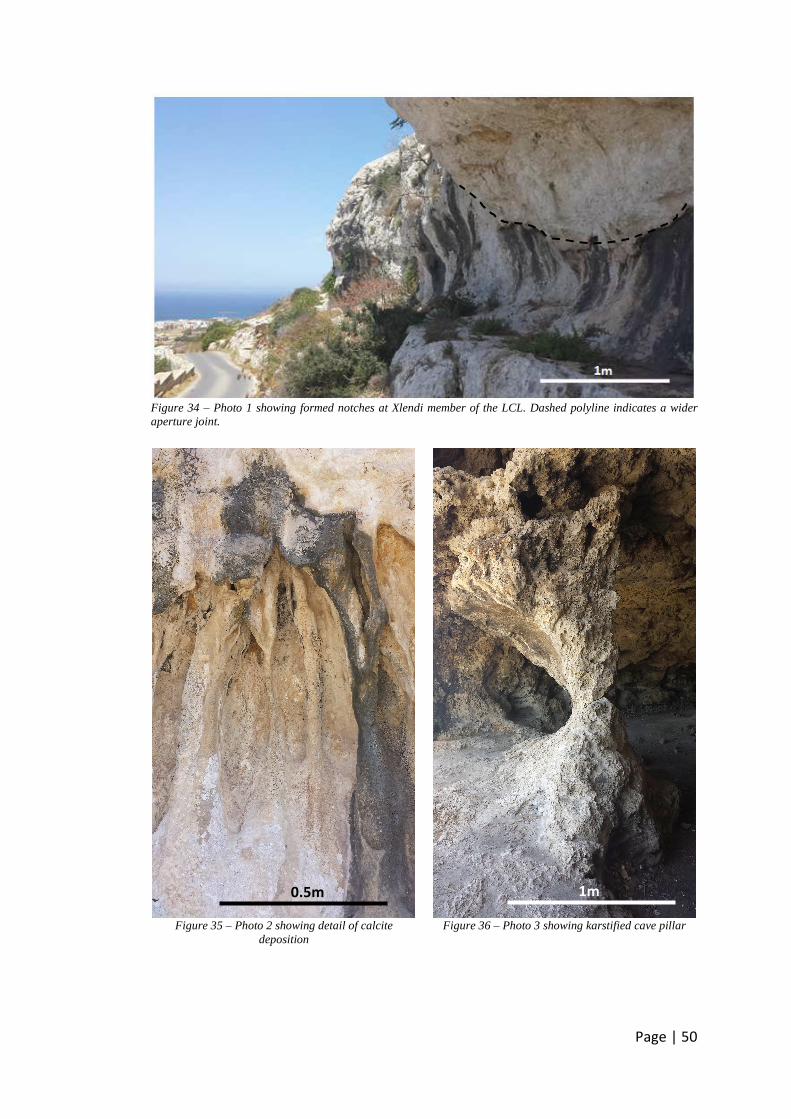
Page | 50

Figure 34 – Photo 1 showing formed notches at Xlendi member of the LCL. Dashed polyline indicates a wider aperture joint.

Figure 35 – Photo 2 showing detail of calcite

deposition

Figure 36 – Photo 3 showing karstified cave pillar

1m 0.5m

Page | 51

4.1.6. St. George’s Bay

Figure 37 – Infilled joint having wide aperture

(scale shown by tape measure)

Figure 38 – Fault Breccia (scale shown by car key)

Figure 39 – Wide open aperture at fault zone

(scale shown by geologic hammer)

Some interesting observations are highlighted from joints and fault zones studied at

St. George’s Bay. The formation here is the LCL and more specifically the Xlendi

member.

A wide joint, at places reaching apertures in the region of two centimetres infilled

with terrarossa traces and zones of calcited walls is shown (Figure 37). This joint

shows at least past fluid flow however at such a state present fluid flow is more

difficult to occur. In such a state fluid flow, if any, would be encouraged to find

easier and wider routes. Such a situation probably results in deviation of fluid flow

paths. Two scenarios are possible in this case either infilling of other joints or

karstification of others. It is believed that this is a function of joint characteristics

such as orientation, aperture, persistence and frequency.

A zone of fault breccias is observed (Figure 38). The cataclasite is angular with some

rounded corners which could have formed during deformation given that the rock is

not very hard. The soil matrix is lighter in colour than that observed in Figure 37 and

also has a good proportion of coarse-grained particles when compared with the

latter. These occurrences can be an indication that at least some of the soil matrix

formed during deformation. The properties of this cataclasite are expected to affect

Page | 52

largely the permeability across and along this joint. Some important properties to

consider are particle size distribution, voids ratio and particle orientation.

Different fault zone architecture with a rock block occupying it is observed (Figure

39). This rock block became dislodged and broken with no evidence of fault breccia.

It is plausible to believe that the fault displacement in the latter case is less than

that for the fault seen in Figure 38 where fault breccias did develop to

accommodate deformation. Unfortunately these interpretations cannot be backed

up by site observations since the height of the outcrop is very short due to past

excavation. In this zone fluid flow is expected to be encouraged through due to

wider aperture.

4.1.7. Msida

The main observations at the Msida site visited are highlighted. A schematic plan

layout of the site is presented (Figure 40). Only minor karst features are observed in

the LGL member (Figure 41). In general the karst features observed in any of the GL

members were not extensive as observed either in the UCL or LCL members. The

major karst feature observed at this site involves a vertical karstified discontinuity

of about 1.5 metres in height (indicated in Figure 44). The discontinuities observed

at the faces of this site are generally grouped in zones which are spaced at between

four and eight metres (Figure 42, Figure 43 and Figure 44). The apertures are

generally tight.

Page | 53

Figure 40 – Schematic plan layout of Excavation site visited at Msida with an indication of the excavation

faces references

Figure 41 – Minor Karst feature noted at wall A

(scale shown by pencil and Barton comb)

Figure 42 – Excavation face A with dotted lines indicating discontinuity zones (scale is shown by excavator)

Page | 54

Figure 43 – Excavation face B with dotted lines indicating discontinuity zones (scale is shown by excavator)

Figure 44 – Excavation face D on the left side, face B on the right side and face C in between. Discontinuity zones are indicated by dotted lines (scale is shown by excavator)

4.1.8. Xghajra

NE striking discontinuities can be widely observed along this part of the coast

(Figure 45 adapted from Google Earth, 2014; Figure 46). The discontinuity at the LGL

wall has a shallower dip angle than that observed in the LCL and thus observations

by Michie et al. (2014) do also apply here. Stretches along the length of the

Page | 55

discontinuities at the LCL outcrop can be observed to be widened by fluid flow and

the surface of the same member is everywhere lightly karstified. This occurrence

was also observed at other UCL outcrops such as at l-Imgiebah. It is plausible to

believe that karst develops mostly at locations of a larger fluid flow.

Figure 45 – Aerial photo of site visited at Xghajra (adapted from Google Earth, 2014). Dashed lines show examples of NE discontinuities which can be observed even from this aerial photo.

An interesting observation at Xghajra is the extremely wide aperture at the contact

between the LGL member and the Il-Mara member of the LCL formation which is in

the region of 200 millimetres (Figure 46; Figure 47). This gives us a good reason to

agree with the interpretation by BRGM (1991b) if this contact is located below the

water table it acts as a fluid conduit.

Remains of the Scutella echinoid bed on top of the LCL forms the transitional bed

between Il-Mara member of the LCL and the LGL (Figure 47; Pedley, 1975).

Page | 56

Figure 46 – Photo 1 showing NE trending

discontinuities on the LGL wall and on the LCL ground (scale shown by field notebook. Dashed lines show discontinuity dip angles. The polyline shows a

karstified stretch on the LCL ground.

Figure 47 – Photo 2 showing contact between LGL

and LCL and Scutella echinoids marker (scale shown by field notebook)

4.1.9. Munxar

The outcrop at the site of Munxar is the MGL (Figure 48). A morphologic difference

between this member and the other two members of the GL can be observed from

the style of surface sub-horizontal discontinuities similar to those observed at

Fomm ir-Rih Bay but better seen here (Figure 49). They seem to be desiccated

discontinuities related with sedimentation processes.

The marly MGL cliff face is very friable (Figure 50).

LCL

LGL

Scutella echinoids

Page | 57

Figure 48 – Aerial photo of Munxar Site (adapted from Google Earth, 2014)

Figure 49 – Photo 2. Dashed lines show examples of tight discontinuities which may be interpreted as

sedimentation desiccation discontinuities. (scale shown by field notebook scale line)

Page | 58

Figure 50 – Photo 1 showing a low MGL cliff face

4.2 Inferring Contacts from Boreholes

4.2.1. UCL/BC

Figure 51 – Investigation boreholes location encircled in red (source: Google Earth, 2014)

300m

Page | 59

It was difficult to closely inspect the UCL/BC geologic contact at the sites visited due

to several toppled rock blocks and debris. For this reason a set of investigation

borehole logs are studied to observe this contact (Appendix C). The set of boreholes

included a set of 12 from a location at the old citadel Mdina (Figure 51; Appendix C).

The description included a sandy material at the UCL/BC contact. This can be either

transported material from the surface through the fracture network or the

greensand material which is reported to be a very thin layer between the UCL and

BC at certain areas.

4.3 Dip (angles) and dip directions of discontinuities

The stereonet plots on which this section is based are attached in Appendix D.

4.3.1. Fomm ir-Rih Bay

The joint sets identified at this site, J1 and J3, closely resemble the two main fault

families of Malta, the ENE-WSW and the NW-SE trending faults respectively.

Interestingly J1 was identified at this site even though the outcrops almost lie at the

footwall of the Victoria fault (ENE-WSW trending). This unbias of the data is

probably the result of the approximate angle between the orientation of the rock

face of the scan lines and the strike of the joint sets being at least 45o. The average

strike of J1 at this site is E-W which closely resembles the orientation of the Victoria

fault at this location. A trend of the bedding is not identified.

At scan line B only few readings were taken due to the short length of the outcrop

at this point and due to the omission of the secondary fractures in between the

main discontinuities (Figure 52). Unarguably the secondary fractures, that form part

of the fault damage zone, increase the permeability of this zone. However they

were omitted from the data collection with the aim to try and identify main

discontinuities trend similarities between the different sites. The readings thus

taken at scan line B are only seven however when they are combined with the

readings for scan line A, 4 of the readings reinforce what is observed in scan line A.

Page | 60

Figure 52 – MGL outcrop at Fomm ir-Rih Bay scan line B. Dashed lines show main joints.

4.3.2. St. George’s Bay

A wide variability of discontinuity data is noted at this site. This can be due and the

close proximity of the site to a mapped fault (the Geological Map of Malta, 1993).

Due to previous excavation works, it is not always easy to identify between main

structural discontinuities and secondary discontinuities. This problem was tackled

by taking a large sample so as to be able to identify the main trends. After

combining all of the data for this site the three main discontinuities are identified.

The most predominant joint set is J5 (bedding) with the dip direction in close

agreement with the mapped direction (the Geological Map of Malta, 1993). The

second most predominant joint set is J1 with an average strike being E-W trending.

This resembles more the strike of the Victoria fault at the west half of Malta rather

than the closest exposure of the Victoria fault which trends approximately ENE-

WSW. The mapped Victoria fault is shown to have a general kink west of Mosta

from a close to an E-W orientation to an ENE-WSW direction (the Geological Map of

Malta, 1993). The third most predominant is J3 which strikes approximately NNW-

SSE at this site. Therefore the two main fault families are also well represented at

this site.

2m

Page | 61

If the scan lines are to be analysed separately it is less evident which joint sets are

the most predominant, however one can note that the highlighted joint sets J2 and

J4 could be antithetic to J1 and J3 respectively. This occurrence closely reflects the

structural geology of Malta with its horst and graben structure. Two other joint sets

J6 and J7 are also observed. J6 probably refers to bedding which dips approximately

NW while J5 dips approximately NE. Being close to a fault zone this variability is

expected.

4.3.3. Msida

The main joint sets identified at Msida are J1 and J2. The average strike of these

sets is closer to the ENE-WSW orientation which closely reflects the trend of a

mapped fault at approximately 1.5 km south of this site (the Geological Map of

Malta, 1993). The discontinuity sample was limited due to the very wide spacing of

discontinuity zones and thus no more clearly dominant discontinuity sets could be

identified. However there seems to be steeply dipping sparse discontinuities

trending approximately NNE-SSW followed by NW-SE trending joints. A trend of the

bedding is not identified.

4.3.4. Xghajra

The main discontinuity sets identified at this site are J5 (bedding) and J1 and J2

which trend approximately NE-SW. The latter two joint sets have approximately the

same average strike but have opposite dip directions with dips that are sub-vertical.

They closely resemble a mapped faults in the vicinity (the Geological Map of Malta,

1993). No dominant discontinuity set sub-parallel to the NW-SE trending mapped

fault (the Geological Map of Malta, 1993) can be identified which probably is due to

the bias imposed by the scan line orientation being sub-parallel to this fault.

Page | 62

A wide dispersal distribution of the poles is observed in scan line A which starts off

very close to a cave-like structure (Figure 53) and undoubtedly has an effect on this

data set. This effect is not noticed at scan line B which was carried out

approximately 75 metres away from scan line A and this structure.

Figure 53 – Cave-like structure adjacent to the position of the start of scan line A

4.3.5. Birkirkara

From all five sites for which discontinuity data is available the data for this site is the

most unclear from a regional tectonic point of view. The main joint set J8 identified

at this site was never identified in any of the other sites. The average dip is shallow

at 25o especially when considering that this joint set is not predominantly made up

of bedding discontinuities. In the other sites it was in general observed that bedding

discontinuities had a very shallow dip angle while the steeper discontinuities

included other joints. From all the sites at which discontinuity data is available, this

site is the furthest away from highly stressed fault zones (Putz-Perrier, 2008; Putz-

Perrier & Sanderson, 2010) and mapped faults (the Geological Map of Malta, 1993).

By looking at a photo of the site (Figure 54) a plausible interpretation might be that

these discontinuities may well be related with the isopach thickening of the LGL

1m

Page | 63

which is reported to be by previous up-arching of this member (Pedley, 1975;

Pedley et al., 1976).

Figure 54 – Photo of Birkirkara site showing undulating discontinuity (scale shown by mobile crane)

4.4 Other discontinuities characteristics

4.4.1. Aperture

Tables showing the population of each joint set per site within each aperture class

are presented (Appendix F). Plots of aperture width class against both dip directions

and dip angles are plotted separately for all the sites, grouped as joint sets and for

the GL formation (Appendix F). The aim is to identify possible trends of wider

apertures. The results are not very clear however some kind of relation is hinted to.

A slight concentration of wider apertures for the E-W trending joint sets are noted

at Fomm ir-Rih Bay, St George’s Bay and Msida and for the N-S trending joint sets at

St. George’s Bay and at Msida (indicated by circles on graphs in Appendix F). Some

West East

Page | 64

apertures seem to increase with increasing dip angle at St. George’s Bay and Msida,

however at St. George’s Bay there are some shallower dips with large apertures too.

Since bedding data is limited, no real comparison of bedding aperture may be made.

At Xghajra and Birkirkara there is no clear trend of wider discontinuities of a

particular joint set. It can be noted that at Birkirkara the apertures are generally on

the wide end of the spectrum.

By plotting the same data and grouping it according to joint sets (Appendix F), it is

noted that the major concentration of wider apertures lies at those joint sets

trending approximately E-W namely J1, J2 and J4. The bedding joint sets (J5, J6, J8

and J10) do not clearly show a trend for aperture. Apertures of the approximately

NNE-SSW trending joint sets J6, J9 and J7 tend to be on the smaller side of the

spectrum with only one joint exceeding aperture class 5. Combining the aperture

data together with the orientations of the latter joint sets may show that the

tectonic origin of the two main fault families of Malta has the least effect on these

joint sets.

No obvious trend could be identified for aperture width in the GL formation mostly

due to the variability across sites. Discontinuities with dip angles ranging from 25o

to 50o are dominated by wider apertures from Birkirkara. At the latter site apertures

are generally on the wider third of the spectrum.

4.4.2. Persistence

Given that the majority of the joints have steep dip angles it is difficult to obtain a

qualitative assessment of persistence from rock outcrop walls with a limited height

such as those studied at Fomm ir-Rih Bay, St. George’s Bay and Xghajra. In such

cases judgement was carried out on what is possible to observe with the

consequence that persistence may be underestimated for some joints. It is

therefore no surprise that most persistence data lies within classes 1 to 3.

Page | 65

Scatter plots for persistence class against dip direction and dip angle, for aperture

width class against persistence class and joint set populations within each

persistence class for each site are presented (Appendix G). The following

observations are made.

At Fomm ir-Rih Bay the higher persistence classes occur for joint sets J1 & J3 having

an ENE-WSW and NW-SE approximate strikes respectively. Some joints with the

higher persistence lie within the joint set J4 but are on the border line of J1. This is

only a matter of grouping and therefore the latter joints may be considered to be

part of J1 too. The apertures of the highest persistent joints tend to be on the

widest end of the spectrum too.

At Msida the higher persistence classes occur for joint sets J1 & J2 which have an

ENE-WSW strike. They are the most occurring joint sets too and reflect one of the

main fault families of Malta. Some of the higher persistence joints lie within joint

set J7 but are a border of joint set J2 and thus may be considered as part of J2 in

this case. The apertures of the most persistent joints vary from very tight to very

wide.

At Birkirkara only three data points have persistence class greater than 3 (circled on

graphs in Appendix G). These joints have similar orientation and dip angles with an

approximate strike of an E-W direction. They lie within two different joint sets J2 &

J8 but at their common border line. These joints have the aperture width class 7

which is almost the largest aperture in this site.

Given the large sample size of St. George’s Bay relatively very few joints have

persistence greater than 3. They are mostly part of the main bedding joint set J5

however they do not have the wider apertures of this site. If we expect to have

higher persistent joints to have the wider apertures the latter occurrence may

highlight clearly the difficulty of this outcrop to gather correct persistence

information.

No clear trend can be identified at Xghajra.

Page | 66

4.4.3. Relative hydraulic conductivity (K)

At Fomm ir-Rih Bay the highest relative K occurs for joint set J4, which has an

average strike approximately ESE-WNW at this site. The second highest relative K

occurs for J3 which strikes approximately NW-SE but is considerably less than J4.

This shows that the relative Ks at this site are tectonically controlled and are highest

for J4 since it has the closest similarity to the nearby Victoria fault. However it

should be reminded that this data set was simplified by not collecting what are

termed as secondary fractures at scan line B (refer to section 4.3.1).

At St. George’s Bay the joint sets J1, J2, J3, J4 and J5 all have similar relative K in the

range from 1.3 to 1.9 mm3/m. These joint sets include the strikes of the two main

fault families of Malta and the bedding.

At Msida all relative Ks for all joint sets are relatively very small due to low joint

frequencies and low average apertures however J1 has the highest relative K. This

again indicates a plausible tectonic control even though the site lies about 1.5

kilometres away from the nearest mapped fault.

At Xghajra the bedding joint set J10 was measured only once however it had a very

high average aperture and thus has the highest relative K. One should remember

the approximately 200mm open GL-LCL contact. J10 may have well been affected by

this contact. The joint sets J7 and J3 follow but have a considerably lower relative K

than J10. They strike approximately NW-SE and again indicate a plausible tectonic

origin.

4.5 Transmissivity

Even though there is a wide scatter of data, transmissivity seems to decrease with

increasing depth below the top of the LCL (Figure 55). Reasons may include the

closure of cracks at depth due to higher vertical stresses, the infill of discontinuities

Page | 67

with transported materials and less occurrence of karst at deeper levels. The

dispersal of data may be explained by knowing that the LCL top is well above mean

sea level at the west while not so at the east coast (refer to structural map of LCL in

Appendix J which is sourced from Pedley, 1975). From west to east members and

lithofacies are probably encountered by the different well tests so one cannot really

generalize for the LCL. For these reasons BRGM (1991b) re-grouped this data by

regions and made some interesting observations. The contact GL-LCL is interpreted

as a conduit of water when located below water and the range between Il-Mara and

Attard members of the LCL is noted to have better productivity (BRGM, 1991b).

Their observations fit in well with the geomorphologic features observed at Xghajra

(Figure 47) and Gharghur (Figure 33, Figure 34, Figure 35 & Figure 36) respectively.

Figure 55 – Variability of transmissivity with borehole depth below top of LCL (line shown is the trend line)

If we consider transmissivity variability with respect to the mean sea level (Figure 56)

one can note that the dispersal of data is less pronounced. Very simply this tells us

that the borehole depths were in general aimed at close to the sea level, however it

may give another piece of information. Transmissivity decreases at a faster rate

with depth below the mean sea level than it does with the depth below the top of

the LCL. This may be an indication of preferential karst features forming close to the

mean sea level given that in mean sea aquifers one expects to have developed karst

Page | 68

near the saline-freshwater contact (Mylroie & Mylroie, 2007), however the basis of

this hypothesis would be very weak if based only on this piece of data.

Figure 56 – Variability of transmissivity with borehole depth with respect to the mean sea level (line shown is the trend line)

Transmissivity is also plotted in relation to proximity to the nearest mapped fault in

the Geological Map of Malta (1993) considered at surface (Figure 57) and at depth

(Figure 58). A good number of data points that have an exceptionally wide scatter

are identified and ignored from the fitting of a possible trend line. It may be that

faults have less of an effect on transmissivity at distances further away than

approximately 600 metres (data points above the red arrow in Figure 57 & Figure

58). Some comparatively low transmissivity values occur relatively close to faults

too (shown circled in Figure 57 & Figure 58). If one ignores these values, there

seems to be a tendency of decreasing transmissivity with distance away from a fault.

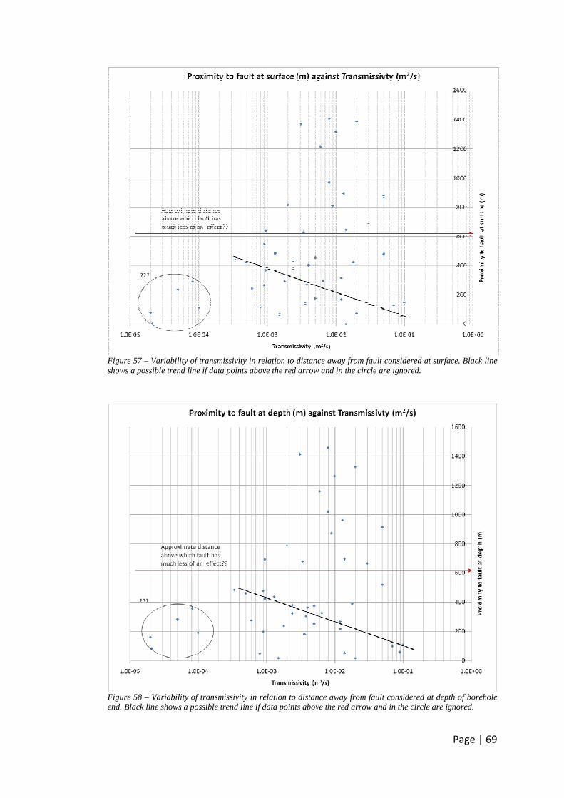
Page | 69

Figure 57 – Variability of transmissivity in relation to distance away from fault considered at surface. Black line shows a possible trend line if data points above the red arrow and in the circle are ignored.

Figure 58 – Variability of transmissivity in relation to distance away from fault considered at depth of borehole end. Black line shows a possible trend line if data points above the red arrow and in the circle are ignored.

Page | 70

Distances at depth between boreholes and faults are worked out by using simple

geometry. The data considered is the topographical level, the borehole depth, the

dip direction of the particular fault being either in the direction or away from the

borehole and by assuming an average fault dip angle of 65o which is approximately

equal to an average fault dip (Appendix I). An interesting observation is the less

scatter of the data shown by the trend line for the plot considering the distance to

the faults at depth (Figure 58). Even though the resolution of the data is low, this

result is encouraging for further investigation on the level of control by faults on the

hydrogeology.

Page | 71

4.6 Potentiometry

Figure 59 – 1990 potentiometric map superimposed on the Geological Map of Malta (1993). Dashed lines show main faults average alignments, dots with number show locations of gauged boreholes with water piezometric level. (adapted from BRGM, 1991c & the Geological Map of Malta, 1993)

The readings of the period 1988 to 1991 are from 40 gauging boreholes which cover

a wide area of Malta (Figure 59). Although this number is not small it is surely not

enough to assess any fault control over water heads. Piezometers close to Il-

Maghlaq fault show the highest levels for readings in proximity to the coast. This

can be due to smeared clays which is known to occur at il-Maghlaq fault (Bonson et

al., 2007), however one should also be aware that the transmissivity for the LCLs at

depths greater than 100 metres below its top are reported to be low (BRGM,

1991b). This may be the case at this location since the top of the LCL here is about

100 metres above sea level (Pedley, 1975).

3km

N

Victoria fault

Il-Maghlaq fault

Page | 72

5 Discussion

The main scope of this chapter is to provide a discussion in a wider context of the

main knowledge acquired from the previous chapters especially from chapter 4. In

so doing the aims reached together with the limitations and further implications are

highlighted. These are then used to recommend future studies.

5.1 Geomorphologic Site Reconnaissance

The quantity of data that is acquired through this simple technique is appreciated.

Even though the extent of this data may not be detailed it provides a good basis as a

qualitative tool which guides further detailed field work and invasive investigation

methods.

5.1.1. Stratal Dip of BC

It is understood that flow in the perched water aquifer of the BC is governed by the

down-dips of the BC stratum. Given that the strata are generally sub-horizontal

large thicknesses of this aquifer are not expected however slightly thicker localised

perched aquifers may occur at the fault drags caused by the ENE-WSW faulting.

These may be spatially limited, not least by a general dip to the east.

This knowledge may be applied to quantify the effects of flow on rock toppling

phenomena (Figure 16; Figure 25) and denser vegetation bands (Figure 21). It is

known that UCL rock toppling failure on top of the BC is triggered by the different

mechanical and hydrogeologic properties of these materials (Gianfranco et al., 2003;

Magri et al., 2008; Devoto et al., 2012).

Further implications to the latter statement include the characterisation of

geomorphologic variability and its correlation with other parameters so as to

Page | 73

characterise these slope instabilities. Possible studies might include the temporal

development of instabilities due to wetting and drying cycles and the combined

effect of discontinuity patterns. The study of desiccation cracks noted at l-Imgiebah

may be included in this study. What happens if the BC is submerged under sea

water? What is the difference from outcropping BC slopes?

5.1.2. Flow indications from karst erosion

It has been observed that karst morphology is a function of grain size of the strata

and their fracturing, with larger developments of karst in coarse-grained strata and

highly fractured zones. Higher developments of karst in coarse-grained strata may

be due to inferior packing of particles and a better connectivity of voids. Other

variables such as flow quantities, the chemical composition such as the calcium

carbonate saturation and the temporal framework of this process are not studied.

In general relatively larger developed karst features are observed in the UCL and

LCL which are coarser-grained (Qammiegh, L-Imgiebah Bay, Fomm ir-Rih Bay, Wied

il-Ghasel, Gharghur and St. George’s Bay). The development of karst within the GL

which are finer-grained is limited in width and generally follows only one direction

along the main wider discontinuities karst features are observed (Qammiegh, L-

Imgiebah, Fomm ir-Rih Bay, Msida, Xghajra, Munxar and Birkirkara).

Karstified caves are noted at a fault zone near Qammiegh (Figure 18) while at

Gharghur karstified notches in the cliff face are noted to develop from a wider

aperture (Figure 34).

Several observations show that fluid conducting boundaries can be found between

layers of different grain size distribution. Perhaps the clearest evidence of this is the

karstified eroded boundary between the GL and LCL observed at Xghajra (Figure 47).

In addition observations of karst features and a dense band of vegetation at

Gharghur close to contacts of members from the same formation indicate that

these fluid conducting boundaries exist even between members or facies within the

Page | 74

same formation (Figure 33). Variation of grain size distributions therefore provides a

barrier to flow into the finer-grained materials at contacts between coarse-grained

and fine-grained materials and encourage flow along these boundaries.

A detailed geomorphologic exercise might identify more of these boundaries and

potentially aid in devising an investigation program to quantify this variability.

Ideally a test programme should aim at obtaining hydraulic data of the different

formations and facies. For Malta this data is widely missing. Further implications of

such an exercise may be the characterisation of geotechnical behaviour of geologic

materials in terms of their nature and state. These properties aid detailed

geotechnical design as for example in quantifying effective stresses.

5.1.3. Sedimentation processes

Sedimentation processes are responsible for various material properties such as

mineralogy, grain size distribution and discontinuities.

In the MGL sub-horizontal discontinuities are interpreted as desiccation

discontinuities along sedimentation boundaries (Figure 30; Figure 49). A study of

sedimentation environments and history may provide more information on more

possible boundaries.

5.1.4. Calcite Deposition

Contrasting observations of karst features and calcite deposition onto rock surfaces

(Figure 35) is evidence of two contrasting affects water can have on carbonates.

This depends on the level of carbonate saturation of the water with respect to the

carbonate content of the particular rock (Fetter, 2001).

Page | 75

The implications are that water may either act to increase or decrease the

permeability by solution processes or calcite deposition respectively. The

characterisation of these processes requires the use of geochemistry.

5.1.5. Style of faulting

St. George’s Bay provides hints on possible joint and fault styles (Figure 37; Figure

38; Figure 39). Hydraulic conductivity depends on the type of discontinuity

developed. Lower hydraulic conductivity is expected for infilled joints and higher

hydraulic conductivity expected for fault zone occupied by fault blocks and open

joints. Fault breccias may reduce the hydraulic conductivity of a fault. The

characterisation of faulting styles and parameters controlling their style are desired.

An antithetic fault is observed at Fomm ir-Rih Bay (Figure 28). Trends of

discontinuities with similar strikes but opposite dip directions are identified in some

of the sites (Appendix E). This may be linked with either faults bounding basins that

are widely observed in the horst and graben of North Malta or may be a matter of

mechanical variabilities of strata and thus their different mode of fracturing (Michie

et al., 2014).

5.2 Discontinuity data

5.2.1. Jointing link with the rifting tectonics of Malta

It is observed that strikes and dip angles of the most occurring joints closely

resemble Malta’s two main fault families being the ENE-WSW and NW-SE trending

faults. The most often identified joint sets are J1 and J2 (ENE-WSW trending)

followed by J3 (NW-SE trend). J1 and J2 are identified at four out of five sites while

J3 is only clearly identified at two of the sites. J3 not being identified at Xghajra is

probably due to the scan line orientation bias as it is oriented close to the NW-SE

direction. At Msida the reason cannot be identified clearly as various orientations

Page | 76

were considered in taking discontinuity data and all visible discontinuities were

measured.

The probable joint origin being the rifting tectonics is also evident from aperture

data. Concentration of data within the wider apertures is observed for joint sets J1,

J2 and J4 which closely resemble an E-W orientation. Joint sets J6, J7 & J9 have

concentration of data within the smaller end of aperture width classes. Their

orientation is approximately NNE-SSW which is furthest away from the orientation

of the main fault families of Malta. This supports a hypothesis that wider apertures

are noted for joints with orientations similar to the orientations of the main faults

of Malta.

Antithetic joint sets appear as trends in various sites. This may be another close link

with the horst and graben structure of Malta.

5.2.2. Limited data from persistence

Some observations from persistence are also possible however it is better not to do

generalizations from this data given the evident data bias from low height of rock

wall outcrops studied.

5.2.3. The case of the Birkirkara site

The case of the Birkirkara site is somewhat different from all the other sites. This

site lies at a distance of about 3 kilometres away from main mapped faults (the

Geological Map of Malta, 1993) while all the other sites lie within 1.5 kilometres of

main faults. Only J8 was identified as a main trending joint set here. J8 has a strike

similar to that of J1 and J2, however its average dip at this site is of 25o which is

shallow when compared to both the averages of J1 and J2 (see Table 7 and Table 8).

J8 reflects a previous event which is reported as up-arching of this member that is

responsible for the thickening of the LGL (Pedley, 1975; Pedley et al., 1976).

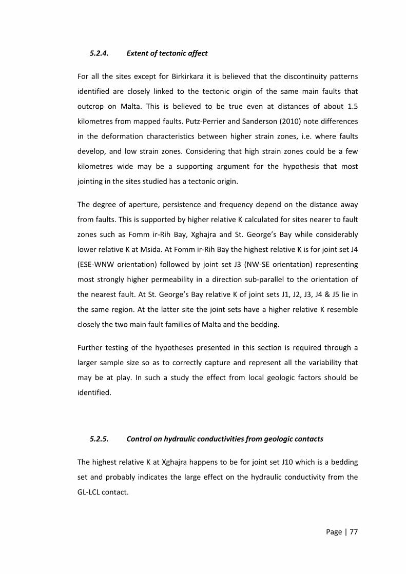
Page | 77

5.2.4. Extent of tectonic affect

For all the sites except for Birkirkara it is believed that the discontinuity patterns

identified are closely linked to the tectonic origin of the same main faults that

outcrop on Malta. This is believed to be true even at distances of about 1.5

kilometres from mapped faults. Putz-Perrier and Sanderson (2010) note differences

in the deformation characteristics between higher strain zones, i.e. where faults

develop, and low strain zones. Considering that high strain zones could be a few

kilometres wide may be a supporting argument for the hypothesis that most

jointing in the sites studied has a tectonic origin.

The degree of aperture, persistence and frequency depend on the distance away

from faults. This is supported by higher relative K calculated for sites nearer to fault

zones such as Fomm ir-Rih Bay, Xghajra and St. George’s Bay while considerably

lower relative K at Msida. At Fomm ir-Rih Bay the highest relative K is for joint set J4

(ESE-WNW orientation) followed by joint set J3 (NW-SE orientation) representing

most strongly higher permeability in a direction sub-parallel to the orientation of

the nearest fault. At St. George’s Bay relative K of joint sets J1, J2, J3, J4 & J5 lie in

the same region. At the latter site the joint sets have a higher relative K resemble

closely the two main fault families of Malta and the bedding.

Further testing of the hypotheses presented in this section is required through a

larger sample size so as to correctly capture and represent all the variability that

may be at play. In such a study the effect from local geologic factors should be

identified.

5.2.5. Control on hydraulic conductivities from geologic contacts

The highest relative K at Xghajra happens to be for joint set J10 which is a bedding

set and probably indicates the large effect on the hydraulic conductivity from the

GL-LCL contact.

Page | 78

5.2.6. Jointing link with nearest fault structure

The ENE-WSW faults have varying strikes ranging from approximately E-W to NE-SW.

If considered at a local level, J1 and J2 closely follow the orientation of the nearest

fault orientation. This occurrence was noted at sites up to approximate distances of

1.5 kilometres away from a fault. However this is not the case for St. George’s Bay

at which site the orientation of J1 is closer to the orientation of the west Victoria

fault portion (Figure 60). A general fault strike kink in the Victoria fault is noted

which also coincides with an isopach thickening of the LGL south of the Victoria

fault at this location (Pedley, 1975). The average orientation of J1 at St. George’s

Bay may indicate that the Victoria fault might have had an effect on a wider zone

than the mapped fault as indicated by its hypothetical extension of the line but may

have been deviated due to some reason such as stress axis orientation or structural

thickening.

Figure 60 – The Victoria fault within the regional geology (adapted from the Geological Map of Malta, 1993)

5.2.7. Further data limitations

For the GL the bedding trend was in general not identified except for the Xghajra

site. A reason for this can be due to the GL being massively bedded (Pedley et al.,

1976) and thus not capturing the bedding trends by biased horizontal scan lines.

Hypothetical extension of

the orientation of the west

Victoria fault portion Average orientation of the

west Victoria fault portion

General fault trend kink

St. George’s Bay

Fomm ir-Rih Bay

En-echelon left-stepping

east Victoria fault portion N

3km

Page | 79

A wide dispersal of data is noted when measurements are in close proximity to

faults or other geologic structures. In such a case, in order to be able to reach a

regional comparison, probably a better approach would be to try and identify the

main geologic structures and hence the causes of the variability within the jointing.

When this cannot be achieved taking many readings as possible to try and obtain

the main trends is a good tool to eliminate as much as possible any data bias.

More trends of spatial variability of jointing within the different geological

formations and facies and within the different geologic contexts should be

identified. These should be backed by statistically significant samples. Ideally this

data should be correlated with field mapping and specifically designed testing

programmes.

5.3 Transmissivity

It is not usual to correlate transmissivity data to distance from faults. This was

carried out at the absence of any more detailed data. Even though a wide dispersal

of data is noted, a certain degree of link between the two seems evident (Figure 57,

Figure 58). At this stage this is an encouraging result considering the wide spatial

area represented by these tests and thus the variability they may represent. Ideally

specific data such as investigation borehole data is to be available so as to be able

to identify possible correlations of data. Such data is probably available at the hands

of the Maltese authorities however no such data is available to this author at the

time of writing this study.

It should also be noted that inferred faults marked as dashed lines of the Geological

Map of Malta (1993) are within a 50 metre accuracy bracket (Pedley, 2014).

Page | 80

5.4 Potentiometry

The potentiometric data available is widely spaced over most of Malta with no

concentration of closely installed piezometers. This does not allow proper analysis

of fault control on the hydraulic properties of the geology of Malta. Given that the

highest reported total heads are in the region between 3 to 5 metres (BRGM, 1991c;

Sapiano et al., 2006) the fault seal control on the hydrogeology is not expected to

be significant however heads depend also on the saltwater-freshwater contact.

5.5 Main Data Limitations

The methods applied and analyses carried out with the data at hand are in no way

exhaustive to understand the full extent of the hydrogeology of Malta. They give a

good indication of what the main controls on hydrogeology are and thus guide

further work.

A good number of sites were visited during the field trip gathering a good spatial

representativeness. Still, most probably they do not encompass the whole

variability of the hydrogeology of Malta. A lot of observations are made, however in

order to support the interpretations a higher number of similar observations across

more sites is desired. Some level of quantification or testing should be done. As a

start, discontinuity data was collected from across five sites.

Confidence in the accuracy of dip angles and dip directions is high. Confidence is

slightly lower for the other discontinuity characteristics since they were visually

taken. However it is still believed that they have a good level of accuracy. As regards

the scan line sample sizes and orientations it was shown that maybe longer scan

lines and more varied orientations are desirable. An improvement on the

discontinuity data set is to include more sites. If a fault such as Victoria fault needs

to be studied in more detail perhaps scan lines along and across the fault at chosen

sites fulfil this requirement. Techniques such as circular scan lines to measure

Page | 81

intensity, density and average length of discontinuities may capture data that is not

captured by linear scan lines.

The major limitation with the analysis carried out with the pre-available data is that

in general the data used may lack specific or complete detail. In the earth sciences

and the geotechnical field a lot of variables and unknowns are involved, so generally

several points of perspectives are desired so as to confirm or otherwise the data.

Possibilities of doing this with the available data are limited. In addition using the

Geological Map of Malta (1993) to measure distances to faults and topographical

levels is expected to result in low confidence outputs.

5.6 Conceptual Ground Model

The area shown is the area chosen for the conceptual ground model presented in

this section (Figure 61). The conceptual ground model (Figure 62) summarises a

good number of observations highlighted in this study.

Figure 61 – Red border shows the area of the conceptual ground model presented in this section (adapted from the Geological Map of Malta, 1993)

N

2km

Fomm ir-Rih Bay

Page | 82

Figure 62 – Conceptual Ground Model highlighting regional hydrogeology of Malta. Annotations cross-referenced to numbers are included on the next page.

Page | 83

1 Displacements of faults towards the east coast probably decrease; therefore

the related fault damage zones narrow down. The synclinal structure due to

the fault drag also narrows down. As displacements decrease towards the east

a wedge-shaped block dipping towards the west is created.

2 Wider fault damage zones to the west of the Victoria Fault.

3 At larger displacements a certain width of damage zones are expected at the

LCL too but still considerably lower than those in the GL (refer to Table 12). For

small throws no damage width is expected within the LCL.

4 Widening of fault damage zones at GL probably increases slip surfaces.

5 BC smear provides a localized seal and compartmentalizes flow parallel to its

direction.

6 Confined Aquifer Zone? BC bottom dipping to a level below sea level

7 Fluid conduit GL-LCL contact. Is this conduit best developed at the saline-fresh

water contact? If yes do we expect a less extensive development of this

contact below sea-level?

8 No seal in NW-SE direction. Il-Maghlaq fault is absent from the coast closest to

this site. Therefore the potential of global aquifer blocks to be sealed by faults

is low. Transmissivity may vary due to variability in facies permeability.

9 Development of karst at GL along fault and subsequently along the sub-

horizontal GL-LCL contact?

10 Is BC seal breached for throws between 5-50 metres as observed by Missenard

et al. (2014)? Karstification of the underlying layers may depend on this.

11 Higher hydraulic conductivity at fault zones and thus lower total heads.

12 Gradual decrease of conductivity away from fault zone as joints apertures

close, frequency decreases and probably persistence decreases too. Higher

total heads (water table) are expected in these zones.

13 More developed karst may form at intersections between faults and sea levels

where highest levels of flow are expected. Vertical infiltration may be

inhibited by the clay cover.

14 The general dip of this wedge to the west is governed by the displacements

being largest to the west. Greater downthrows occur towards the west.

15 Valleys are formed dipping to the east in an approximate west-east direction.

Their occurrence is governed by the general dip of strata to the east and

probably by the ENE-WSW trending faults. Solution subsidence structures may

aid the development of valleys.

16 Springs

17 Sandy contact between the ULC and BC.

Page | 84

6 Summary and Conclusions

6.1 Main Conclusions

The main findings of this research work on the structural controls on the

hydrogeology of Malta are summarised.

The potentiometric data available is widely spaced over most of Malta with no

concentration of closely installed piezometers. This makes proper analysis of fault

seal control on the hydrogeology of Malta impossible. Evidenced in part by low

highest heads of about 3 to 5 metres, large aquifer blocks controlled by fault seals

are probably inexistent. Fault seals may be existent along a limited uni-directional

stretch.

Possibilities of fault parameters such as displacements to define the fault

architecture were previously shown (Michie et al., 2014). Hydraulic conductivity is

expected to vary depending on the type of discontinuity developed whether being

an infilled joint, made up of fault blocks and open joints or fault breccias.

In general the joints are shown to be closely linked to the latest rift tectonics of

Malta. This is evidenced from similar strikes and dip angles of the most occurring

joints that closely resemble the ENE-WSW and NW-SE trending faults, the wider

apertures of these joints and the relative K calculated. Even joints at distances of

about 1.5 kilometres away from mapped faults are shown to be linked with the rift

tectonics as their orientations closely resemble the nearest fault structures. A

decrease in aperture width and spacing is observed at locations away from the

faults. Confirmation or otherwise of this hypothesis should be tackled by collecting

a statistically significant sample.

The site of Birkirkara presents a somewhat different situation from all the other

sites. This site lies at a distance of about 3 kilometres away from the nearest

mapped faults (the Geological Map of Malta, 1993). The main trending joint set

identified, J8, shows strike similarity to the ENE-WSW trending faults but occurs at a

Page | 85

much shallower dip. This may show that rift tectonics do not have or have less of an

affect at these distances away and/or shows evidence of previous events that may

have been up-arching effects that are responsible for the isopach thickening of the

LGL (Pedley, 1975; Pedley et al., 1976).

From observations it is noted that karst development differs between formations or

facies that exhibit variability in grain size distribution and fracturing. Perhaps more

specifically coarse-grained strata may have inferior packing of particles and a better

connectivity of voids. Both of these two characteristics increase the hydraulic

conductivity of a rock mass. Therefore larger developments of karst are expected in

rock masses of higher hydraulic conductivities. In addition observations highlight

that fluid conducting boundaries can result between layers of different grain size

distributions. An erosive contact of the GL-LCL boundary at Xghajra is observed.

Sedimentation processes may be responsible for various material properties such as

grain-size distributions and discontinuities.

It is not usual to correlate transmissivity data to distance from faults especially

when the data is of low resolution. However even though a wide dispersal of data is

noted, a certain degree of correlation between the two seems plausible. This result

provides encouragement for future research.

6.2 Further Studies

6.2.1. Fault parameters and control

The further study of fault architecture is encouraged along and across faults by

carrying out field mappings. Data gaps still exist by missing inland data. Correlations

from findings may shed light on hydraulic characterisation of faults. Techniques

such as linear and circular scan lines are deemed to aid the initial quantification.

A next step would be to design a field and laboratory testing programme so as to

correlate hydraulic properties to the geologic contexts identified. Methods to

Page | 86

correlate investigation data at depth with surface data are to be found. In so doing

data may be extrapolated to predict hydraulic behaviour at sites where data is still

limited. This data would then be subject to further future testing.

6.2.2. Controls on jointing

More trends of spatial variability of jointing within the different geological

formations and the different geologic contexts should be tested by statistically

significant samples. Sample sites should preferably be chosen with the hydrological

cycle in mind.

6.2.3. Permeability variability of different formations and facies

In this study controls on fluid flow paths due to formations or facies having varying

grain size distributions of the geological strata has been identified. The zoning of

such strata combined by intact rock and rock mass permeability testing would

provide useful information for characterising the hydrogeology of Malta. For Malta

this data is widely missing.

If this data is combined with geotechnical properties of geologic materials both in

terms of their nature and state useful information in quantifying effective stresses

for engineering purposes may be reached.

6.2.4. Geochemistry

Both observations of carbonate solution and calcite deposition have been observed.

The geochemical processes at play have a governing effect on the hydraulic

properties of such zones. Analysis of flow paths from geomorphology in

combination with geochemical testing are deemed to provide a useful tool in

characterising possible geochemical controls on the hydrogeology of Malta.

Page | 87

References

Alexander, D. (1988) A review of the physical geography of malta and its significance

for tectonic geomorphology. Quaternary Science Reviews. 7 (1), 41-53.

Argnani, A. (1990) The strait of sicily rift zone: Foreland deformation related to the

evolution of a back-arc basin. Journal of Geodynamics. 12 (2–4), 311-331.

Anzidei, M., Baldi, P., Casula, G., Galvani, A., Mantovani, E., Pesci, A., Riguzzi, F. &

Serpelloni, E. (2001) Insights into present-day crustal motion in the central

Mediterranean area from GPS surveys. Geophys. J. Int. 146, 98-110.

ATIGA. (1972) Wastes disposal and water supply project in Malta. Malta, UNDP.

Bakalowicz, M. & Mangion, J. (2003) The limestone aquifers of Malta: Their

recharge conditions from isotope and chemical surveys. IAHS-AISH Publication.

(278), 49-54.

Bonson, C. G., Childs, C., Walsh, J. J., Schöpfer, M. P. J. & Carboni, V. (2007)

Geometric and kinematic controls on the internal structure of a large normal fault in

massive limestones: The Maghlaq Fault, Malta. Journal of Structural Geology. 29 (2),

336-354.

Bosence, D. W. J. & Pedley, H. M. (1982) Sedimentology and palaeoecology of a

Miocene coralline algal biostrome from the Maltese Islands. Palaeogeography,

Palaeoclimatology, Palaeoecology. 38 (1–2), 9-43.

Bureau de Recherche Géologique et Minière (BRGM). (1991) Study of the fresh-

water resources of Malta. Executive Summary. Malta, Government of Malta.

Bureau de Recherche Géologique et Minière (BRGM). (1991b) Study of the fresh-

water resources of Malta. Appendix 2. Hydrodynamic characteristics. Malta,

Government of Malta.

Page | 88

Bureau de Recherche Géologique et Minière (BRGM). (1991c) Study of the fresh-

water resources of Malta. Appendix 4. Potentiometry of the mean sea level aquifer.

Malta, Government of Malta.

British Standards Institution (1999) BS 5930:1999. Code of practice for site

investigations. London, BSI.

Cartwright, J. A., Trudgill, B. D. & Mansfield, C. S. (1995) Fault growth by segment

linkage: an explanation for scatter in maximum displacement and trace length data

from the Canyonlands Grabens of SE Utah. Journal of Structural Geology. 17 (9),

1319-1326.

Debono, G. & Xerri, S. (1993) Geological Map of the Maltese Islands. 1:25000. Sheet

1 - Malta. Malta, Oil Exploration Directorate, Office of the Prime Minister.

Dart, C. J., Bosence, D. W. J. & McClay, K.R. (1993) Stratigraphy and structure of the

Maltese graben system. Journal of the Geological Society. 150, 1153-1166.

Dawers, N. H. & Anders, M. H. (1995) Displacement-length scaling and fault linkage.

Journal of Structural Geology. 17 (5), 607-614.

Devoto, S., Biolchi, S., Bruschi, V., M., Furlani, S., Mantovani, M., Piacentini, D.,

Pasuto, A. & Soldati, M. (2012) Geomorphological map of the NW Coast of the

Island of Malta (Mediterranean Sea). Journal of Maps. 8 (1), 33-40.

Faerseth, R. B. (2006) Shale smear along large faults: continuity of smear and the

fault seal capacity. Journal of the Geological Society, London. 163, 741-751.

Fetter, C. W. (2001) Applied Hydrogeology. Fourth Edition. New Jersey, USA,

Prentice-Hall, Inc.

Gardiner, W., Grasso, M. & Sedgeley, D. (1995) Plio-pleistocene fault movement as

evidence for mega-block kinematics within the Hyblean—Malta Plateau, Central

Mediterranean. Journal of Geodynamics. 19 (1), 35-51.

Page | 89

Gianfranco, M., Samori, L., Ragazzini, A., Cuppini, G. & Baratin, L. (2003)

Consolidamento del Palazzo Vilhena - M'dina (Malta) - Relazione geotecnica.

Bologna, Universita` di Bologna. Report number: 6.

Gillespie, P. A., Walsh, J. J. & Watterson, J. (1992) Limitations of dimension and

displacement data from single faults and the consequences for data analysis and

interpretation. Journal of Structural Geology. 14 (10), 1157-1172.

Gonzalez de Vallejo, L. I. & Ferrer, M. (2011) Geological Engineering. London, CRC

Press.

Google. (2014) Google Earth [computer programme] Google Inc.

Illies, J. H. (1981) Graben Formation - The Maltese Islands - a case history.

Tectonophysics. 73, 151-168.

Jongsma, D., Woodside, J. M., King, G. C. P. & van Hinte, J. E. (1987) The Medina

Wrench: a key to the kinematics of the central and eastern Mediterranean over the

past 5 Ma. Earth and Planetary Science Letters. 82 (1–2), 87-106.

Kim, Y., Peacock, D. C. P. & Sanderson, D. J. (2003) Mesoscale strike-slip faults and

damage zones at Marsalforn, Gozo Island, Malta. Journal of Structural Geology. 25

(5), 793-812.

Magri, O., Mantovani, M., Pasuto, A. & Soldati, M. (2008) Geomorphological

investigation and monitoring of lateral spreading along the north-west coast of

Malta. Geogr. Fis. Dinam. Quat. 31, 171-180.

Marrett, R. & Allmendinger, R. W. (1990) Kinematic analysis of fault-slip data.

Journal of Structural Geology. 12 (8), 973-986.

Ministry for European Affairs (2014) CF120: National Flood Relief Project (NFRP).

[Online] Available from: https://investinginyourfuture.gov.mt/project/waste-

Page | 90

management-and-risk-prevention/national-flood-relief-project-nfrp-42041344

[Accessed 11th August 2014].

Mylroie, J. R. & Mylroie, J. E. (2007) Development of the carbonate island karst

model. Journal of Cave and Karst Studies. 69 (1), 59-75.

Micarelli, L., Benedicto, A. & Wibberley, C. A. J. (2006) Structural evolution and

permeability of normal fault zones in highly porous carbonate rocks. Journal of

Structural Geology. 28 (7), 1214-1227.

Michie, E. A. H., Haines, T. J., Healy, D., Neilson, J. E., Timms, N. E. & Wibberley, C. A.

J. (2014) Influence of carbonate facies on fault zone architecture. Journal of

Structural Geology. 65 (0), 82-99.

Missenard, Y., Bertrand, A., Vergély, P., Benedicto, A., Cushing, M. & Rocher, M.

(2014) Fracture-fluid relationships: implications for the sealing capacity of clay

layers–Insights from field study of the Blue Clay formation, Maltese islands. Bulletin

De La Societe Geologique De France. 185 (1), 51-63.

Newbery, J. (1968) The perched water table in the upper limestone aquifer of

Malta. Journal of the Institution of Water. 22, 551-570.

Newbery, J. (1976) Miocene sea-floor subsidence and later subaerial solution

subsidence structures in the Maltese Islands. Proceedings of the Geologists'

Association. 87 (1), 111.

Pedley, H. M. (1975) The Oligo-Miocene sediments of the Maltese Islands. PhD. The

University of Hull.

Pedley, H. M. (1975b) Miocene Sea-floor Subsidence and Later Subaerial Solution

Subsidence Structures in the Maltese Islands. Proc. Geol. Ass. 85 (4), 533-547.

Page | 91

Pedley, H. M. (1987) Controls on Cenozoic carbonate deposition in the Maltese

Islands: review and reinterpretation. Memorie Della Societa Geologica Italiana. 38,

81-94.

Pedley, H. M. (1990) Syndepositional tectonics affecting Cenozoic and Mesozoic

deposition in the Malta and SE Sicily areas (Central Mediterranean) and their

bearing on Mesozoic reservoir development in the N Malta offshore region. Marine

and Petroleum Geology. 7 (2), 171-180.

Pedley, M. (1998) A review of sediment distributions and processes in Oligo-

Miocene ramps of southern Italy and Malta (Mediterranean divide). Geological

Society, London, Special Publications. 149, 163-179.

Pedley, M. (2011) The Calabrian Stage, Pleistocene highstand in Malta: a new

marker for unravelling the Late Neogene and Quaternary history of the islands.

Journal of the Geological Society, London. 168, 913-925.

Pedley, Martyn. Geologist. (Personal communication, 6th August 2014).

Pedley, H. M., House, M. R. & Waugh, B. (1976) The geology of Malta and Gozo.

Proceedings of the Geologists' Association. 87 (3), 325-341.

Pedley, H. M. & Bennett, S. M. (1985) Phosphorites, hardgrounds and

syndepositional solution subsidence: A palaeoenvironmental model from the

miocene of the Maltese Islands. Sedimentary Geology. 45 (1-2), 1-34.

Pratt, S. K. (1990) Hardground genesis in pelagic carbonates from the Miocene of

Malta and Cretaceous of Southern England. PhD. University of London.

Putz-Perrier, M. W. (2008) Distribution and Scaling of Extensional Strain in

Sedimentary Rocks. PhD. Imperial College of Science, Technology and Medicine, UK.

Page | 92

Putz-Perrier, M. W. & Sanderson, D. J. (2010) Distribution of faults and extensional

strain in fractured carbonates of the North Malta Graben. The American Association

of Petroleum Geologists. 94 (4), 435-456.

Reuther, C. -D. & Eisbacher, G. H. (1985) Pantelleria Rift - crustal extension in a

convergent intraplate setting. Geologische Rundschau. 74 (3), 585-597.

Rocscience Inc. (2004), Dips Version 5.1 - Graphical and Statistical Analysis of

Orientation Data. www.rocscience.com, Toronto, Ontario, Canada. [Computer

program].

Sapiano, M., Mangion, J. and Batchelor, C. (2006) Water Resources Review. Rome,

FAO. Report number: 1.

Sapiano, Manuel. Head of water policy unit within MRA. (Personal communication,

31st July 2014).

Seebeck, H., Nicol, A., Walsh, J. J., Childs, C., Beetham R. D. & Pettinga, J. (2014)

Fluid flow in fault zones from an active rift. Journal of Structural Geology. 62, 52-64.

Snow, D. T. (1970) The frequency and apertures of fractures in rock. J. Rock Mech.

Min. Sci. 7, 23-40.

Stuart, M. E., Maurice, L., Heaton, T. H. E., Sapiano, M., Micallef Sultana, M.,

Gooddy, D. C. & Chilton, P. J. (2010) Groundwater residence time and movement in

the Maltese islands – A geochemical approach. Applied Geochemistry. 25 (5), 609-

620.

Trechmann, C. T. (1938) Quaternary Conditions in Malta. The Geological Magazine.

75 (1), 1-26.

Watterson, J. (1986) Fault Dimensions, Displacements and Growth. Pageoph. 124,

365-373.

Page | 93

Appendix A – The Geological Map of Malta (1993)

Page | 94

Page | 95

Appendix B – Main water bodies as indicated by the Malta Resources

Authority (MRA)

Groundwater Body Code

MT001

Groundwater Body Name

Malta Main Mean Sea Level Groundwater Body

Reference Year

2004

General Characteristics

Location

The Malta Main Mean Sea Level Groundwater Body is sustained in the Lower Coralline Limestone aquifer and is in free contact with sea-water. This groundwater body extends over the whole southern and central parts of the Island, under the Rabat Dingli Plateau, The Mgarr Plateau, the Wardija Ridge up to the Pwales Valley as its northern boundary. In real terms the Groundwater Body can be compared to a lens-shaped body of fresh-water floating on more saline water, with a thickness of fresh-water below sea-level approximately thirty-six times its piezometric height above sea level.

Area 217km2

Main Aquifer Lower Coralline Limestone

Main Aquifer Type Fractured Carbonate Media

Groundwater Horizon 1; 2 in the western regions

Maximum Length 21km

Maximum Width 13km

Mathematical centre of groundwater body 450600, 3971400

Hydro-geological characteristics

Stratigraphy Tertiary—Oligocene

Mean Annual Precipitation 543mm

Mean Groundwater Body Thickness 67.5m

Main Recharge Source Precipitation

Mean Annual Recharge 34.3hm3

Pressures

Main Land-Use Features (Corinne Landcover 2000)

Discontinuous urban fabric 23%

Other Pressures

Water Abstraction Purpose Potable Supply, Irrigation, Secondary Domestic and Industrial

Contaminated Land Old un-lined landfill sites at Maghtab, Wied Fulija and Luqa

Possible Associated Aquatic Ecosystems Is-Salina, Il-Maghluq (Marsascala), Il-Ballut (Marsaxlokk) L-Ghadira s-Safra

Agriculture with significant area of natural vegetation 43%

Schlerophyllous vegetation 6%

Sparsely Vegetated areas 3%

Airport 2%

Mineral abstraction sites 1%

Areas overlain by perched aquifers 17%

Industrial zones 4%

Artificial Recharge Mainly due to leakages from the potable supply and sewerage network

Page | 97  

 

Page | 98  

 

Page | 99  

 

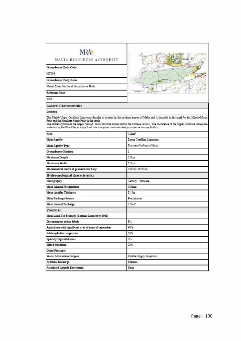
Page | 100  

 

Page | 101  

 

Page | 102  

 

Page | 103  

 

Page | 104  

 

 

 

 

Page | 105

Appendix C – Mdina investigation boreholes from Gianfranco et al.

(2003)

Page | 106

Page | 107

Page | 108

Page | 109

Page | 110

Page | 111

Page | 112

Page | 113

Page | 114

Page | 115

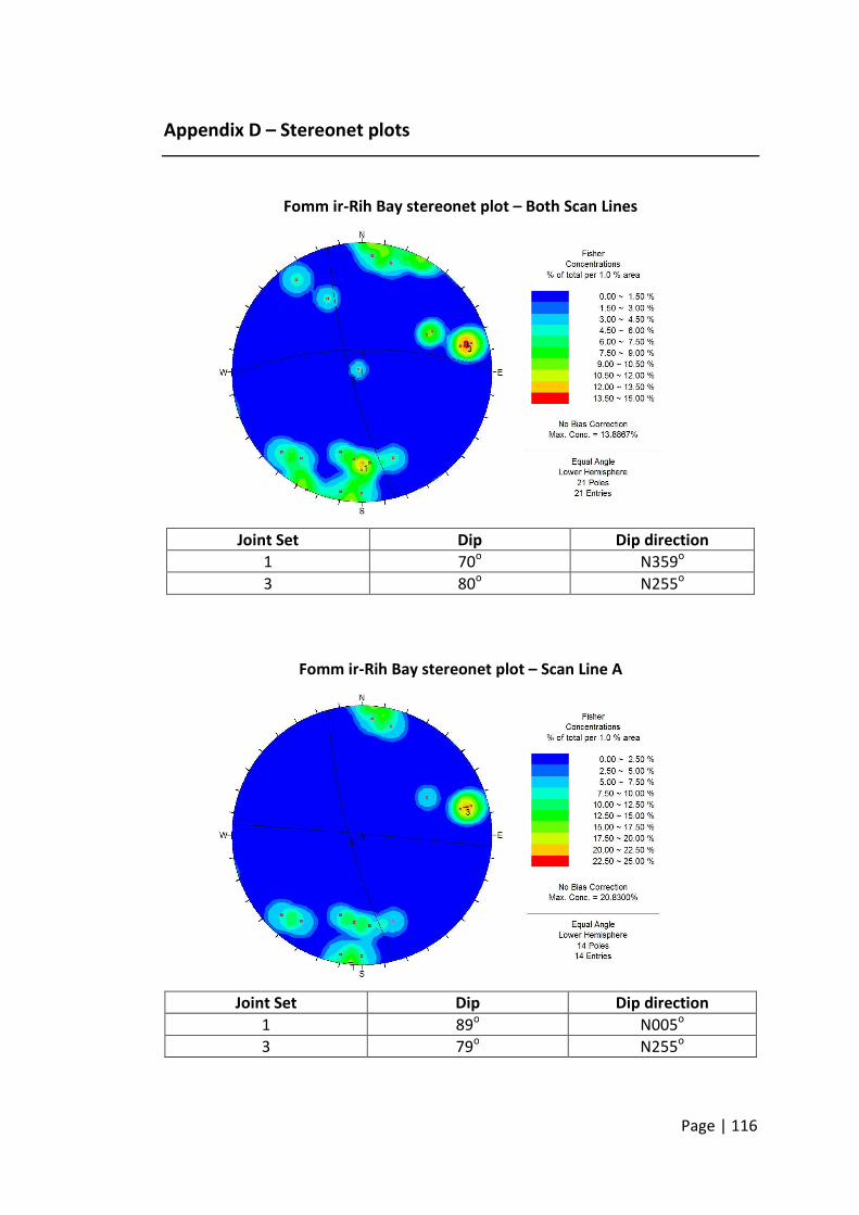
Page | 116

Appendix D – Stereonet plots

Fomm ir-Rih Bay stereonet plot – Both Scan Lines

Joint Set Dip Dip direction

1 70o N359

o

3 80o N255

o

Fomm ir-Rih Bay stereonet plot – Scan Line A

Joint Set Dip Dip direction

1 89o N005

o

3 79o N255

o

Page | 117

Fomm ir-Rih Bay stereonet plot – Scan Line B

Page | 118

St. George’s Bay stereonet plot – All Scan Lines

Joint Set Dip Dip direction

1 86o N356

o

3 66o N259

o

5 (bedding) 11o N057

o

St. George’s Bay stereonet plot – Scan Line A

Joint Set Dip Dip direction

1 86o N356

o

3 58o N237

o

5 (bedding) 12o N060

o

Page | 119

St. George’s Bay stereonet plot – Scan Line B

Joint Set Dip Dip direction

1 80o N353

o

2 84o N192

o

3 68o N258

o

6 (bedding??) 9o N314

o

St. George’s Bay stereonet plot – Scan Line C

Joint Set Dip Dip direction

2 68o N158

o

3 70o N217

o

4 89o N031

o

5 (bedding) 20o N045

o

7 74o N117

o

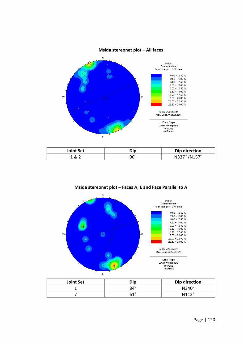
Page | 120

Msida stereonet plot – All faces

Joint Set Dip Dip direction

1 & 2 90o N337

o /N157

o

Msida stereonet plot – Faces A, E and Face Parallel to A

Joint Set Dip Dip direction

1 84o N340

o

7 61o N113

o

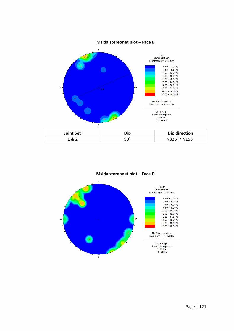
Page | 121

Msida stereonet plot – Face B

Joint Set Dip Dip direction

1 & 2 90o N336

o / N156

o

Msida stereonet plot – Face D

Page | 122

Xghajra stereonet plot – Both Scan Lines

Joint Set Dip Dip direction

1 85o N325

o

2 85o N149

o

5 (bedding) 5o N056

o

Xghajra stereonet plot – Scan Line A

Joint Set Dip Dip direction

2 87o N144

o

5 (bedding ??) 13o N090

o

Page | 123

Xghajra stereonet plot – Scan Line B

Joint Set Dip Dip direction

1 83o N324

o

2 83o N152

o

5 (bedding) 5o N045

o

Page | 124

Birkirkara stereonet plot – All Scan Lines

Joint Set Dip Dip direction

8 25o N174

o

Birkirkara stereonet plot – Scan Line A

Joint Set Dip Dip direction

8 22o N180

o

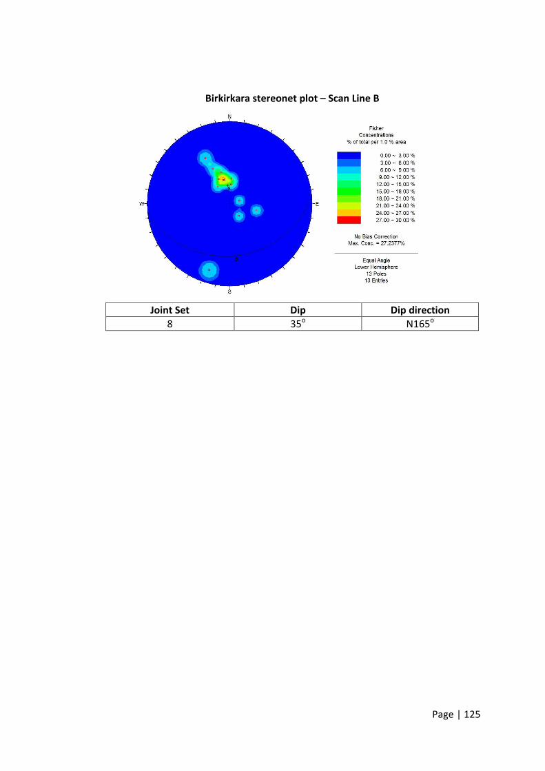
Page | 125

Birkirkara stereonet plot – Scan Line B

Joint Set Dip Dip direction

8 35o N165

o

Page | 126

Appendix E – Full scan lines sheets

Page | 127

Fomm ir-Rih Discontinuity Scan Lines (letter in first column refers to scan line and number to position in metres)

Page | 128

St George’s Bay Discontinuity Scan Line A (letter in first column refers to scan line and number to position in metres)

Page | 129

Page | 130

Page | 131

Page | 132

St George’s Bay Discontinuity Scan Line B (letter in first column refers to scan line and number to position in metres)

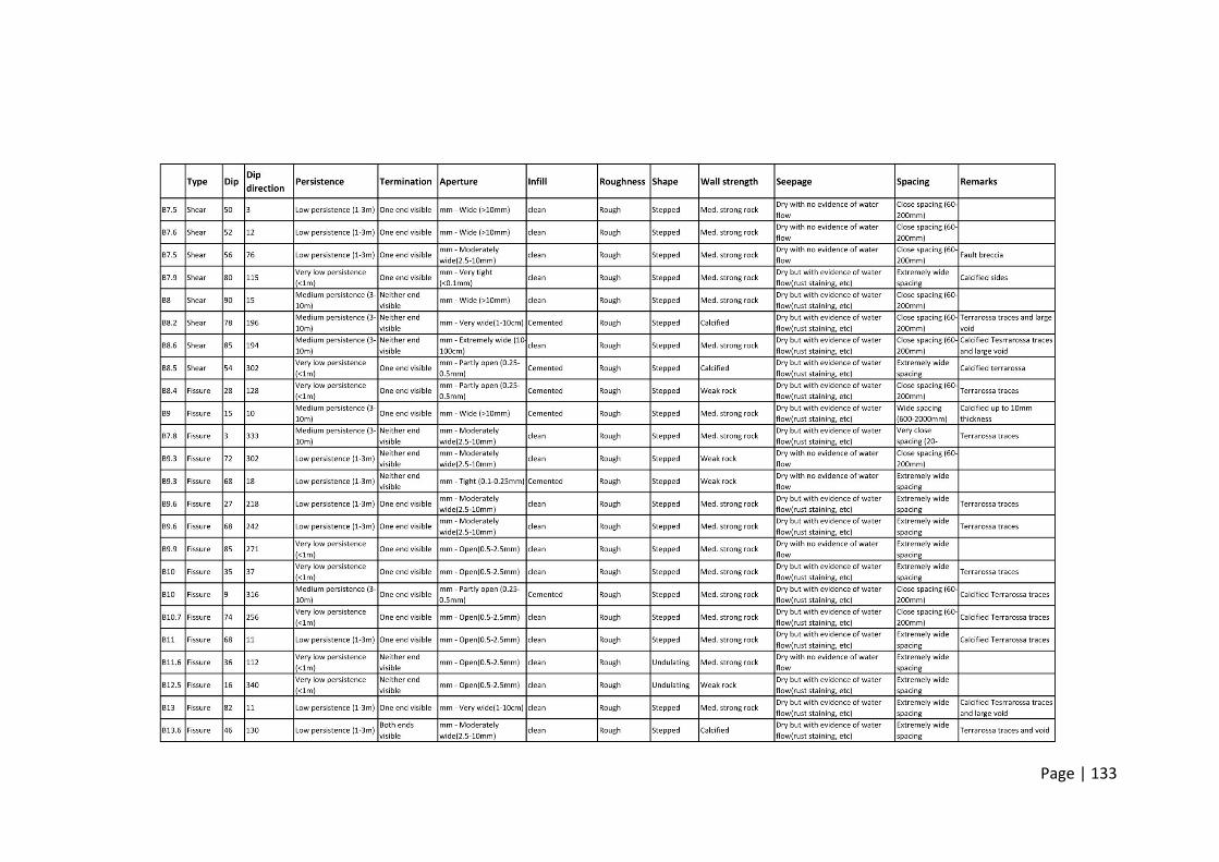
Page | 133

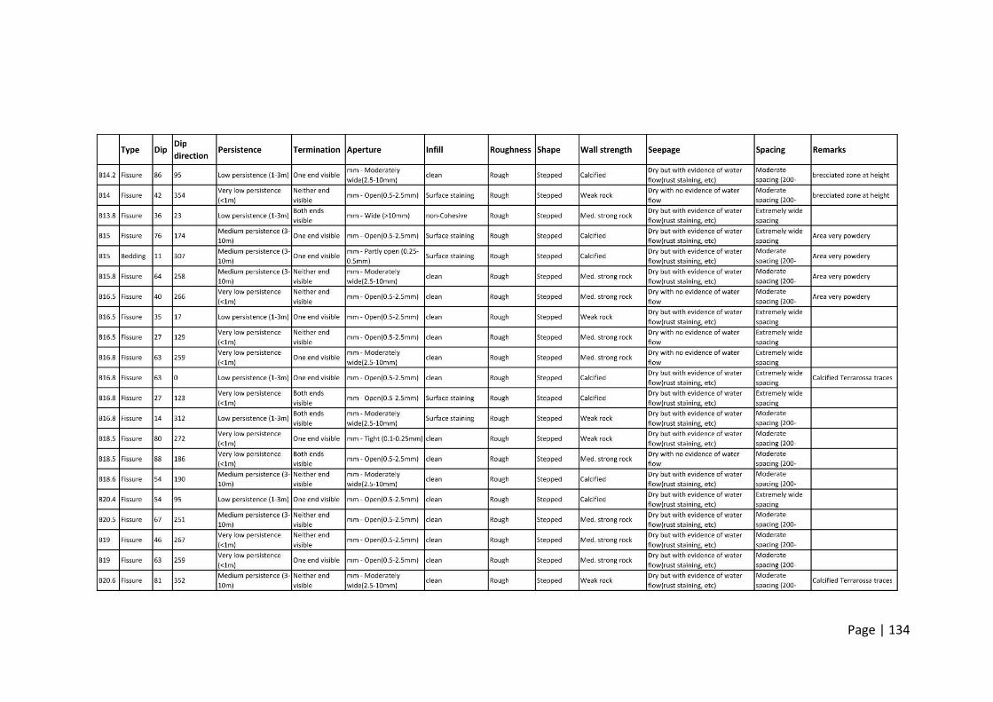
Page | 134

Page | 135

St George’s Bay Discontinuity Scan Line C (letter in first column refers to scan line and number to position in metres)

Page | 136

Page | 137

Page | 138

Msida Discontinuity Faces A & E (letter in first column refers to face and number refers to reading entry)

Page | 139

Msida Discontinuity Faces B & C (letter in first column refers to face and number refers to reading entry)

Page | 140

Msida Discontinuity Face D (letter in first column refers to face and number refers to reading entry)

Page | 141

Xghajra Discontinuity Scan Line A (letter in first column refers to scan line and number to position in metres)

Page | 142

Xghajra Discontinuity Scan Line B (letter in first column refers to scan line and number to position in metres)

Page | 143

Birkirkara Discontinuity Face A (letter in first column refers to face and number refers to reading entry)

Page | 144

Birkirkara Discontinuity Face B (letter in first column refers to face and number refers to reading entry)

Page | 145

Appendix F – Tables and graphs of discontinuities aperture data

Fomm ir-Rih Bay – Aperture class frequencies for each joint set

Joint Set

/

Aperture

J1 J2 J3 J4 J5 J6 J7 J8 J9 J10

1

2 1

3 1 1

4 2 2 1

5 1 1

6 1 3

7

8

Totals 3 3 2 5 1

Fomm ir-Rih Bay – Aperture class percentages for each joint set

Joint Set

/

Aperture

J1 J2 J3 J4 J5 J6 J7 J8 J9 J10

1

2 33.3

3 33.3 50

4 66.7 40 100

5 33.3 33.3

6 50 60

7

8

Totals 100 100 100 100

100

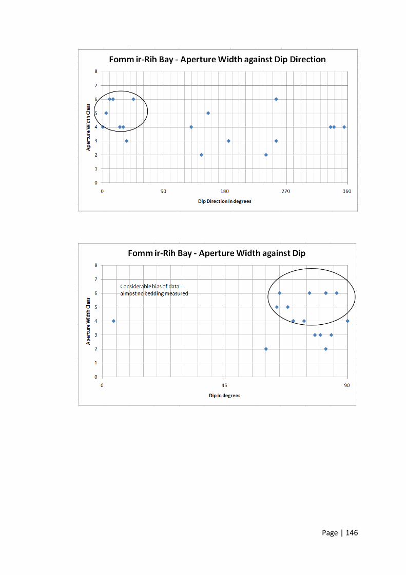
Page | 146

Page | 147

St George Bay – Aperture class frequencies for each joint set

Joint Set

/

Aperture

J1 J2 J3 J4 J5 J6 J7 J8 J9 J10

1 5 1 4 1 1 1

2 6 1 7 8 9 1 5 1 2

3 2 4 3 3 4 3 2 1 2

4 11 11 14 13 6 4 5 4 5 1

5 5 4 6 7 11 7 3 1 1 2

6 2 1 5 2

7 2 3 1 2 1 1

8 2 2

Totals 35 26 32 38 37 16 14 9 9 6

St George Bay – Aperture class percentages for each joint set

Joint Set

/

Aperture

J1 J2 J3 J4 J5 J6 J7 J8 J9 J10

1 14.3 3.1 10.8 6.3 7.1 11.1

2 17.1 3.8 21.9 21.1 24.3 6.3 35.7 11.1 22.2

3 5.7 15.4 9.4 7.9 10.8 18.8 22.2 11.1 33.3

4 31.4 42.3 43.8 34.2 16.2 25.0 35.7 44.4 55.6 16.7

5 14.3 15.4 18.8 18.4 29.7 43.8 21.4 11.1 11.1 33.3

6 5.7 3.8 13.2 5.4

7 5.7 11.5 3.1 5.3 2.7 16.7

8 5.7 7.7

Totals 100 100 100 100 100 100 100 100 100 100

Page | 148

Page | 149

Msida – Aperture class frequencies for each joint set

Joint Set

/

Aperture

J1 J2 J3 J4 J5 J6 J7 J8 J9 J10

1 4 8 1 4 2 1

2 4 4 1 1 3 1

3 3

4 1

5 1 1

6 1

7 2 1

8

Totals 14 15 2 6 5 2

Msida – Aperture class percentages for each joint set

Joint Set

/

Aperture

J1 J2 J3 J4 J5 J6 J7 J8 J9 J10

1 28.6 53.3 50 66.7 40 50

2 28.6 26.7 50 16.7 60 50

3 21.4

4 6.7

5 7.1 6.7

6 16.7

7 14.3 6.7

8

Totals 100 100 100 100

100

100

Page | 150

Page | 151

Xghajra – Aperture class frequencies for each joint set

Joint Set

/

Aperture

J1 J2 J3 J4 J5 J6 J7 J8 J9 J10

1

2 1 1

3 1 1 1

4 2 2 1 1

5 1 1 1 1

6 1 1 1 1

7

8

Totals 2 4 1 2 1 3 2 3 1

Xghajra – Aperture class percentages for each joint set

Joint Set

/

Aperture

J1 J2 J3 J4 J5 J6 J7 J8 J9 J10

1

2

50 33.3

3 50 25

33.3

4

50

100 100

33.3

5

25 100

33.3

33.3

6 50

33.3 50

100

7

8

Totals 100 100 100 100 100

100 100 100 100

Page | 152

Page | 153

Birkirkara - Aperture class frequencies for each joint set

Joint Set

/

Aperture

J1 J2 J3 J4 J5 J6 J7 J8 J9 J10

1

2 1

3 1 1

4 2 2

5 1 4 2 2 1 1 4 3 3

6 1 1 2

7 1 3 1 1 3 2

8 1

Totals 4 7 2 7 2 1 0 10 3 8

Birkirkara - Aperture class percentages for each joint set

Joint Set

/

Aperture

J1 J2 J3 J4 J5 J6 J7 J8 J9 J10

1

2 25

3

10

12.5

4

28.6

20

5 25 57.1 100 28.6 50 100

40 100 37.5

6 25

14.3

25

7 25 42.9

14.3 50

30

25

8

14.3

Totals 100 100 100 100 100 100

100 100 100

Page | 154

Page | 155

Page | 156

Page | 157

Page | 158

Page | 159

Page | 160

Page | 161

Page | 162

Appendix G – Tables and graphs of discontinuities persistence data

Fomm ir-Rih Bay – Persistence class frequencies for each joint set

Joint Set

/

Persistence

J1 J2 J3 J4 J5 J6 J7 J8 J9 J10

1 1

2 2 2 2 4

3 1 1

4 3 1 2

5

Totals 5 3 4 6 1

Fomm ir-Rih Bay – Persistence class percentages for each joint set

Joint Set

/

Persistence

J1 J2 J3 J4 J5 J6 J7 J8 J9 J10

1 100

2 40 66.7 50 66.7

3 33.3 25

4 60.0 25 33.3

5

Totals 100 100 100 100

100

Page | 163

& J4

& J4

Page | 164

St. George’s Bay – Persistence class frequencies for each joint set

Joint Set

/

Persistence

J1 J2 J3 J4 J5 J6 J7 J8 J9 J10

1 15 11 20 13 12 2 5 4 6 2

2 17 10 10 22 17 7 9 4 3 3

3 4 5 2 2 5 7 1 1

4 1 2

5 1

Totals 36 26 32 38 37 16 14 9 9 6

St. George’s Bay – Persistence class percentages for each joint set

Joint Set

/

Persistence

J1 J2 J3 J4 J5 J6 J7 J8 J9 J10

1 41.7 42.3 62.5 34.2 32.4 12.5 35.7 44.4 66.7 33.3

2 47.2 38.5 31.3 57.9 45.9 43.8 64.3 44.4 33.3 50.0

3 11.1 19.2 6.3 5.3 13.5 43.8 11.1 16.7

4 2.6 5.4

5 2.7

Totals 100 100 100 100 100 100 100 100 100 100

Page | 165

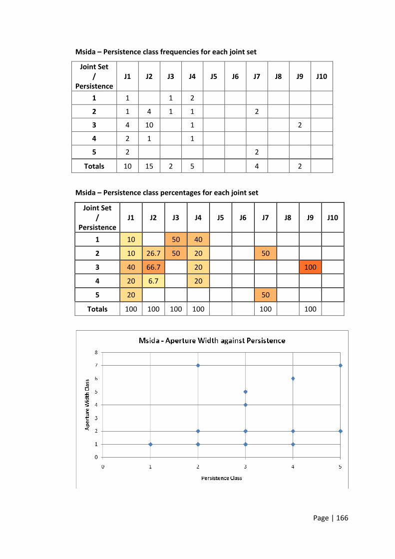
Page | 166

Msida – Persistence class frequencies for each joint set

Joint Set

/

Persistence

J1 J2 J3 J4 J5 J6 J7 J8 J9 J10

1 1 1 2

2 1 4 1 1 2

3 4 10 1 2

4 2 1 1

5 2 2

Totals 10 15 2 5 4 2

Msida – Persistence class percentages for each joint set

Joint Set

/

Persistence

J1 J2 J3 J4 J5 J6 J7 J8 J9 J10

1 10 50 40

2 10 26.7 50 20 50

3 40 66.7 20 100

4 20 6.7 20

5 20 50

Totals 100 100 100 100

100

100

Page | 167

Page | 168

Xghajra – Persistence class frequencies for each joint set

Joint Set

/

Persistence

J1 J2 J3 J4 J5 J6 J7 J8 J9 J10

1 1 1 1

2 1 4 1 1 1 1 2 1

3 1 1

4 1

5

Totals 2 4 1 2 1 3 1 3 1

Xghajra – Persistence class percentages for each joint set

Joint Set

/

Persistence

J1 J2 J3 J4 J5 J6 J7 J8 J9 J10

1 50 33.3 33.3

2 50 100 100 50 100 33.3 66.7 100

3 50 100

4 33.3

5

Totals 100 100 100 100 100

100 100 100 100

Page | 169

Page | 170

Birkirkara - Persistence class frequencies for each joint set

Joint Set

/

Persistence

J1 J2 J3 J4 J5 J6 J7 J8 J9 J10

1 1 5 1 3 2

2 1 3 1 1 2 4

3 3 4 1 2 1 6 2

4

5 1 2

Totals 4 8 2 8 2 1 10 3 8

Birkirkara - Persistence class percentages for each joint set

Joint Set

/

Persistence

J1 J2 J3 J4 J5 J6 J7 J8 J9 J10

1 50 62.5 100 100 25

2 25 37.5 12.5 50 20 50

3 75 50 50 25 50 60 25

4

5 12.5 20

Totals 100 100 100 100 100 100

100 100 100

Page | 171

Page | 172

Appendix H – Relative hydraulic conductivities

Fomm ir-Rih Bay - Relative Hydraulic Conductivity for each joint set

Joint

Set

Number of

readings, n

Length of

scan line,

L (m)

Frequency,

λi (m-1

)

Average

Aperture,

ei (mm)

ei3

(mm3)

Relative

Ki

(mm3/m)

J1 6 14.1 0.43 1.5 3.375 1.436

J2 4 14.1 0.28 0.375 0.053 0.015

J3 4 14.1 0.28 8.9375 713.918 202.530

J4 6 14.1 0.43 17.5 5359.375 2280.585

J5

J6

J7

J8 1 14.1 0.07 1.5 3.375 0.239

J9

J10

St. George's Bay - Relative Hydraulic Conductivity for each joint set

Joint

Set

Number of

readings, n

Length of

scan line,

L (m)

Frequency,

λi (m-1

)

Average

Aperture,

ei (mm)

ei3

(mm3)

Relative

Ki

(mm3/m)

J1 36 68.3 0.53 1.5 3.375 1.779

J2 26 68.3 0.38 1.5 3.375 1.285

J3 32 68.3 0.47 1.5 3.375 1.581

J4 38 68.3 0.56 1.5 3.375 1.878

J5 37 68.3 0.54 1.5 3.375 1.828

J6 16 68.3 0.23 1.5 3.375 0.791

J7 14 68.3 0.20 1.5 3.375 0.692

J8 9 68.3 0.13 1.5 3.375 0.445

J9 9 68.3 0.13 1.5 3.375 0.445

J10 6 68.3 0.09 1.5 3.375 0.296

Page | 173

Msida - Relative Hydraulic Conductivity for each joint set

Joint

Set

Number of

readings, n

Length of

scan line,

L (m)

Frequency,

λi (m-1

)

Average

Aperture,

ei (mm)

ei3

(mm3)

Relative

Ki

(mm3/m)

J1 15 107.9 0.14 0.175 0.005 0.00075

J2 16 107.9 0.15 0.05 0.000 0.00002

J3 2 107.9 0.02 0.1125 0.001 0.00003

J4 6 107.9 0.06 0.05 0.000 0.00001

J5

J6

J7 5 107.9 0.05 0.175 0.005 0.00025

J8

J9 2 107.9 0.02 0.1125 0.001 0.00003

J10

Xghajra - Relative Hydraulic Conductivity for each joint set

Joint

Set

Number of

readings, n

Length of

scan line,

L (m)

Frequency,

λi (m-1

)

Average

Aperture,

ei (mm)

ei3

(mm3)

Relative

Ki

(mm3/m)

J1 7 29.5 0.24 0.375 0.053 0.013

J2 13 29.5 0.44 1.5 3.375 1.487

J3 1 29.5 0.03 6.25 244.141 8.276

J4 2 29.5 0.07 1.5 3.375 0.229

J5 6 29.5 0.20 1.5 3.375 0.686

J6 1 29.5 0.03

J7 4 29.5 0.14 6.25 244.141 33.104

J8 3 29.5 0.10 0.175 0.005 0.001

J9 3 29.5 0.10 0.375 0.053 0.005

J10 1 29.5 0.03 17.5 5359.375 181.674

Page | 174

Appendix I – Hydrodynamic data

Page | 175

Compiled table used for the re-interpretation of Transmissivity (BRGM, 1991b; Sapiano, 2014)

Page | 176

Page | 177

Page | 178

Data points used shown on the Geologic Map of

Malta (1993).

First number is the ID number of the well

borehole and the second number is the

transmissivity in m2/s. Both values are

referenced with the tables presented.

Each square is a 1 x 1 km square.

N

Page | 179

Appendix J – Fault data and structural contours of LCL

Page | 180

Fitting of data points to determine an equation in the form of

– Section 3.6.1

In the following working is represented by the letter and is represented by .

The general equation of a parabola is , where , and are

constants such that . Hence substituting the three points ,

and in the general equation, the following three equations

will be produced:

Equation (1):

Equation (2):

Equation (3):

Solving equations (2) and (3) simultaneously:

The following Equation (4) is obtained by multiplying Equation (2) by .

Equation (4):

Equation (3):

Equation (4) – Equation (3):

Substituting the value of in Equation (3) we get .

Page | 181

Hence, the equation is

The above quadratic equation is graphically shown as follows:

Research shows that the relationship between displacement ( ) and length of fault

( ) is of the form , where is a constant not equal to zero (Watterson,

1986; Cartwright et al., 1995). Hence, by adjusting the above quadratic equation by

varying the coefficient of and fixing the coefficient of equal to zero, we get the

approximation . The negative sign of the coefficient

of and intercept are insignificant, as they only translate the graph on a

different position on the axes and do not alter the shape of the graph. Graphically

the adjusted equation is shown below.

Page | 182

Table showing fault data extracted from the Geological Map of Malta (1993)

Name of section Section A-A` of The Geological Map of Malta

Line-

trend 170 deg. from North

Fault

Number

Distance

[m]

Dip

direction

[o

from

N.]

Actual

Dip

[o]

Measured

throw

[m]

Actual

Throw

[m]

App.

Heave

[m]

Corr.

Heave

[m]

Displacement

[m] Fault

START 0.00 - - - - - -

1 1,085.88 1 62.2 80.63 32.25 17.31 16.99 36.45

2 1,372.46 167 57.0 278.76 111.50 72.6 72.50 133.00 Qammiegh

3 1,771.53 341 66.0 17.46 6.98 3.15 3.11 7.65

4 2,403.42 144 71.2 94.07 37.63 14.29 12.84 39.76

5 3,020.52 315 59.2 58.06 23.22 16.87 13.82 27.02

6 3,911.21 333 65.3 49.04 19.62 9.45 9.04 21.60

7 4,232.21 163 71.9 86.46 34.58 11.38 11.30 36.38

8 4,331.73 163 72.7 155.42 62.17 19.46 19.31 65.10

9 5,527.27 172 73.2 119.65 47.86 14.46 14.45 49.99

10 6,087.94 340 60.5 114.77 45.91 26.42 26.02 52.77

11 6,319.83 350 57.8 81.45 32.58 20.49 20.49 38.49

12 6,743.00 165 61.8 21.17 8.47 4.56 4.54 9.61

13 7,377.05 355 66.9 25.99 10.40 4.45 4.43 11.30

14 7,498.86 167 75.8 10.06 4.02 1.02 1.02 4.15

15 7,854.30 199 65.4 61.98 24.79 12.99 11.36 27.27

16 9,086.62 1 61.8 452.45 180.98 98.93 97.11 205.39 Victoria

17 9,301.60 142 63.6 18.20 7.28 4.1 3.62 8.13

18 10,333.65 146 72.2 47.54 19.02 6.7 6.12 19.98

19 10,638.03 331 63.9 17.16 6.86 3.56 3.37 7.64

20 11,525.99 157 62.6 28.11 11.24 5.98 5.83 12.66

21 13,014.22 335 63.9 10.10 4.04 2.05 1.98 4.50

Page | 183

Fault geometry (sourced from Michie et al., 2014) – Section 3.6.2

Calculation of FSZ width using geometry from Michie et al. (2014)

a 67 deg. (average from Michie et al., 2014)

b 80 deg. (average from Michie et al., 2014)

x 60.0 m (GL thickness from Pedley, 1975)

wh 102.3 m

h 35.7 m

wf 25.5 m

FSZ 163.4 m

However FSZ width is expected to be wider than this due to

presence of BC and UCL too at this point. So let us say not less than

200 metres.

Page | 184

Predictive equations for damage zones width against displacement (sourced from

Michie et al., 2014)

Page | 185

Calculations of damage zones widths using the predictive equations in the

previous page for Table 12 (sourced from Michie et al., 2014)

Heave 10 m

Fault dip 74 deg. (avg. for GL and LCL formations - Michie et al., 2014)

Displacement 36.3 m

Formation GL LCL

FSZ (m) 22.2 2.1 15.3

(range for LCL between 2.1m

and 15.3m)

TDZ (m) 71.2 14.3

Avg. Fault core (m) 0.6