Embed Size (px)
Citation preview

Universität Karlsruhe (TH)Institut für Theoretische Informatik
Diplomarbeit
Scheduling and Topology Control inWireless Sensor Networks
Markus Völker
30. Oktober 2008
Betreut durch:
Universität Karlsruhe:Dipl.-Inform. Bastian KatzProf. Dr. Dorothea Wagner
Carnegie Mellon University:Ass.-Prof. Dr. Willem-Jan van HoeveProf. Dr. R. Ravi


Acknowledgements
First of all, I want to thank my supervisors Bastian Katz and Prof. Wagner (Univer-sity of Karlsruhe), as well as Ass.-Prof. van Hoeve and Prof. Ravi (Carnegie MellonUniversity), for all their help and support! In particular, I would like to thank Prof.Wagner for the opportunity to write my thesis at her institute, and for supporting myapplication for the interACT exchange program. As well, I want to thank Prof. vanHoeve and Prof. Ravi for the very obliging supervision and care during my time atCarnegie Mellon University. My most profound thanks go to Bastian Katz, for pointingme to the topic of sensor networks and for the great support and the helpful assistancethroughout my work on this thesis.
I am much obliged to Agilent Technologies for the financial support during my studies.At this point, I also want to sincerely thank Stefan Weiss and Markus Walter for theirsupport! Moreover, I am very grateful to the people behind the interACT exchangeprogram for making my stay abroad possible.
Finally, I would like to thank Lars Hofer, Matthias Thoma, and Tatiane Utumi forproofreading this thesis, and Viswanath Nagarajan for useful discussions.
This thesis is dedicated to my parents, Alfred and Maria Völker.
Hiermit versichere ich, dass ich die vorliegende Arbeit selbständig angefertigt habe undnur die angegebenen Hilfsmittel und Quellen verwendet wurden.
Karlsruhe, den 30. Oktober 2008
Unterschrift: ........................................
1

Abstract
Within recent years, wireless sensor networks became a very popular tool for distributedmonitoring of various physical and environmental conditions. Thanks to the ongoingminiaturization of the required hardware, this trend is likely to continue. In this the-sis, we study the problems of scheduling and topology control in wireless networks.We consider both, networks with fixed transmission powers, and networks with freelyadjustable transmission powers. For the scheduling problem, several methods for thecomputation of optimum schedules, as well as the computation of upper and lowerbounds on the length of optimum schedules, are presented and analyzed. Additionally,various possibilities for optimizing the proposed methods are described. All methodshave been implemented and are used in an experimental section, to gain additional in-sights into the properties of wireless networks. Subsequently, the scheduling heuristicsare extended to topology control algorithms. Goal of this topology control algorithmsis the computation of topologies whose links can be scheduled efficiently. At the sametime, the resulting topologies are required to conserve certain properties of the orig-inal network, such as connectivity or spanner properties. Furthermore, we propose asimple topology control algorithm that works local and does not require any informa-tion about node positions. The proposed topology control algorithms are compared tovarious existing algorithms, using several quality measures for network topologies.
A central part of this thesis is dedicated to the evaluation of constraint programmingas a tool for solving scheduling problems based on the physically motivated SINR inter-ference model. For this purpose, constraint programming is compared to integer linearprogramming, and several experiments are performed to highlight the pros and cons ofboth approaches. The constraint programs have been solved using the freely availableGecode solver, which is described to some detail in the beginning of this thesis.
2

Contents
1 Introduction 7
2 Preliminaries 112.1 Graphs and Networks . . . . . . . . . . . . . . . . . . . . . . . . . . . . 112.2 Mathematical Programming . . . . . . . . . . . . . . . . . . . . . . . . . 12
2.2.1 Linear Programming . . . . . . . . . . . . . . . . . . . . . . . . . 132.2.2 Integer Programming . . . . . . . . . . . . . . . . . . . . . . . . . 14
2.3 Constraint Programming . . . . . . . . . . . . . . . . . . . . . . . . . . . 142.3.1 Notations and Definitions . . . . . . . . . . . . . . . . . . . . . . 15
2.4 Gecode: Generic Constraint Development Environment . . . . . . . . . 162.4.1 Models and Constraints . . . . . . . . . . . . . . . . . . . . . . . 172.4.2 Propagators and Filtering . . . . . . . . . . . . . . . . . . . . . . 182.4.3 Search Engines for CSPs and COPs . . . . . . . . . . . . . . . . 192.4.4 Branchings . . . . . . . . . . . . . . . . . . . . . . . . . . . . . . 202.4.5 Performance Measures . . . . . . . . . . . . . . . . . . . . . . . . 212.4.6 Extending Gecode . . . . . . . . . . . . . . . . . . . . . . . . . . 212.4.7 C++ Interface vs. Java Interface . . . . . . . . . . . . . . . . . . 22
3 Survey on Wireless Sensor Networks 233.1 Communication Graphs . . . . . . . . . . . . . . . . . . . . . . . . . . . 233.2 How to deal with Interference . . . . . . . . . . . . . . . . . . . . . . . . 253.3 Scheduling Problem . . . . . . . . . . . . . . . . . . . . . . . . . . . . . 263.4 Interference Models . . . . . . . . . . . . . . . . . . . . . . . . . . . . . . 27
3.4.1 SINR Model . . . . . . . . . . . . . . . . . . . . . . . . . . . . . . 283.4.2 Conflict Graphs and Graph-based Interference Models . . . . . . 293.4.3 Graph-based Models vs. SINR Model . . . . . . . . . . . . . . . 31
3.5 Topology Control . . . . . . . . . . . . . . . . . . . . . . . . . . . . . . . 323.5.1 Quality Criteria for Topologies . . . . . . . . . . . . . . . . . . . 33
3.6 Related Results . . . . . . . . . . . . . . . . . . . . . . . . . . . . . . . . 34
4 Scheduling 374.1 Power Control . . . . . . . . . . . . . . . . . . . . . . . . . . . . . . . . . 374.2 Exact Scheduling Algorithms . . . . . . . . . . . . . . . . . . . . . . . . 40
4.2.1 Constraint Programming . . . . . . . . . . . . . . . . . . . . . . 40
3

Contents
4.2.1.1 Fixed Transmission Power . . . . . . . . . . . . . . . . . 404.2.1.2 Variable Transmission Power . . . . . . . . . . . . . . . 444.2.1.3 Optimizations . . . . . . . . . . . . . . . . . . . . . . . 45
4.2.2 Integer Linear Programming . . . . . . . . . . . . . . . . . . . . . 484.2.2.1 Fixed Transmission Power . . . . . . . . . . . . . . . . . 494.2.2.2 Variable Transmission Power . . . . . . . . . . . . . . . 514.2.2.3 Additional Objectives . . . . . . . . . . . . . . . . . . . 53
4.3 Scheduling Heuristics . . . . . . . . . . . . . . . . . . . . . . . . . . . . . 544.3.1 Fixed Transmission Power: MaxSINR . . . . . . . . . . . . . . . 544.3.2 Variable Transmission Power: MinPower . . . . . . . . . . . . . . 56
4.4 Computation of Lower Bounds for Optimum Schedules . . . . . . . . . . 57
5 Topology Control 615.1 Overview of existing Algorithms and Topologies . . . . . . . . . . . . . . 61
5.1.1 Gabriel Graph and Relative Neighborhood Graph . . . . . . . . . 625.1.2 LIFE and LISE . . . . . . . . . . . . . . . . . . . . . . . . . . . 635.1.3 Minimum Spanning Tree Algorithms . . . . . . . . . . . . . . . . 635.1.4 Cone Based Topology Control (CBTC) . . . . . . . . . . . . . . . 645.1.5 XTC Algorithm . . . . . . . . . . . . . . . . . . . . . . . . . . . . 64
5.2 Topologies which can be efficiently scheduled . . . . . . . . . . . . . . . 655.2.1 MaxSINR Topology and MinPower Topology . . . . . . . . . . . 655.2.2 MinInterference Topology . . . . . . . . . . . . . . . . . . . . . . 675.2.3 Constraint Programming . . . . . . . . . . . . . . . . . . . . . . 68
6 Experimental Results 716.1 Implementation and Testing Environment . . . . . . . . . . . . . . . . . 716.2 Parameters used for the SINR Model . . . . . . . . . . . . . . . . . . . . 726.3 Scheduling . . . . . . . . . . . . . . . . . . . . . . . . . . . . . . . . . . . 73
6.3.1 Test data . . . . . . . . . . . . . . . . . . . . . . . . . . . . . . . 736.3.2 Graph-based Models vs. SINR Model . . . . . . . . . . . . . . . 756.3.3 Analysis of Optimum Schedules . . . . . . . . . . . . . . . . . . . 766.3.4 Variable Power vs. Fixed Power . . . . . . . . . . . . . . . . . . . 806.3.5 Quality of Heuristic and Lower Bound . . . . . . . . . . . . . . . 826.3.6 Performance . . . . . . . . . . . . . . . . . . . . . . . . . . . . . . 846.3.7 Solution Quality . . . . . . . . . . . . . . . . . . . . . . . . . . . 866.3.8 Random Restarts . . . . . . . . . . . . . . . . . . . . . . . . . . . 87
6.4 Topology Control . . . . . . . . . . . . . . . . . . . . . . . . . . . . . . . 906.4.1 Quality Measures . . . . . . . . . . . . . . . . . . . . . . . . . . . 906.4.2 Test Data and considered Topologies . . . . . . . . . . . . . . . . 926.4.3 Visual Comparison based on a single Sample . . . . . . . . . . . 936.4.4 Comparison based on a Series of Samples . . . . . . . . . . . . . 986.4.5 Similarities between the Topologies . . . . . . . . . . . . . . . . . 103
4

Contents
7 Final Remarks 1057.1 Mathematical Programming vs. Constraint Programming . . . . . . . . 1067.2 Outlook . . . . . . . . . . . . . . . . . . . . . . . . . . . . . . . . . . . . 107
8 Zusammenfassung (German abstract) 109
List of Figures 111
List of Tables 112
List of Algorithms 112
Bibliography 113
5

6

1 Introduction
Networks of small sensor nodes, so-called sensor networks, consist of spatially dis-tributed autonomous devices which use sensors to cooperatively monitor physical orenvironmental conditions, such as pressure, temperature or vibration, at different lo-cations. Originally, the development of sensor networks was motivated by militaryapplications such as battlefield surveillance. However, the ongoing miniaturization ofthe sensor nodes as well as the availability of cheaper and cheaper hardware led to anabundance of new applications, including habitat and environment monitoring, indus-trial machinery surveillance, healthcare and home automation.
Today, the smallest sensor nodes already have a diameter of only about one millimeter.Yet, there is no end in sight for the miniaturization and it is hoped that soon the sensornodes will be small and cheap enough that thousands of them can be scattered inorder to work cooperatively. This concept became known as smartdust [18] because thedevices are intended to be only the size of a dust particle. Of course, these applicationsput high demands on the used hardware and software. Due to their tiny size, sensornodes cannot be equipped with big batteries. Moreover, in many applications it isimpossible to recharge or replace sensor nodes that run out of power. Therefore, energyconservation is very crucial in the context of sensor networks.
Since energy is the limiting factor of lifetime and operability of most ad-hoc networks,there has been a lot of research on how to conserve energy in sensor networks. Oneof the approaches proposed so far is topology control. The basic idea behind topologycontrol is to restrict the network topology, the structure of links connecting pairs ofnetwork nodes, to a small connecting subset of all possible links in order to make routingon the topology faster and easier. Moreover, the energy needed for a transmissionstrongly depends on the distance between sender and receiver. The energy requiredfor communication between two sensor nodes grows at least quadratically with theirdistance. Therefore, avoiding large-distance links usually helps to conserve energy.
Most of the theoretical work on sensor networks is based on oversimplified graph-basedmodels. These models neither adequately take into account the dependence betweentransmission quality and sender-receiver-distance, nor do they consider that sensornodes that are not within transmission range also interfere to a certain extent witheach other. For this reason, this thesis relies on the more sophisticated SINR model, aphysically motivated radio propagation model.
The main goals of this thesis are: providing efficient heuristics for the computation of
7

1 Introduction
good upper and lower bounds on the length of optimal schedules in wireless networks,to develop and study optimized methods for the computation of exact schedules, to usethe aforementioned methods to analyze differences and similarities between differentmodels for sensor networks, to propose new topology control algorithms which try tominimize the number of slots that are necessary to schedule all links of the generatedtopologies, to compare this topology control algorithms with existing algorithms, and,last but not least, to evaluate constraint programming and compare it to integer linearprogramming based on the experiments that were performed in the context of thisthesis.
Organization of this thesis
In the following, we give a brief chapter outline in order to provide a quick overview onthe organization of this thesis.
Chapter 2: The second chapter provides the reader with the necessary backgroundknowledge that is not directly connected to wireless sensor networks. It startswith some basic notations and definitions in the field of graph theory. Subse-quently, the techniques mathematical programming and constraint programmingare introduced. As most of the readers are probably not so familiar with constraintprogramming, this topic is covered in more detail. The chapter is concluded witha detailed description of Gecode, the constraint programming solver that is usedfor the experiments in this thesis.
Chapter 3: A brief survey on sensor networks is given. First, it is shown how networktopologies can be modeled using communication graphs. Two famous kinds ofcommunication graphs, namely unit disk graphs and quasi unit disk graphs, aredescribed. Next, different ways of how the medium access layer of the networkcan deal with interference and resulting transmission failures are shown. This isfollowed by the definition of the scheduling problem, one of the main topics of thisthesis. Subsequently, a brief overview on how interference in wireless networkscan be modeled is given. Graph based models of interference, as well as the moreprofound SINR model, are introduced and compared to each other. At this, theuse of the SINR model is motivated. Finally, the topology control problem isintroduced.
Chapter 4: The fourth chapter is dedicated to the scheduling problem. It starts withthe question how one can decide if a set of transmissions can be scheduled atthe same time, and how one can determine optimal transmission powers suchthat all transmissions satisfy the SINR constraint without wasting energy. Af-terwards, constraint programs (CPs) and integer linear programs (ILPs) for the
8
computation of optimum solutions of the scheduling problem are given. To pushup the size of exactly solvable problems, several optimizations for the CPs andILPs are discussed. However, real world instances of the scheduling problem areintractable with exact algorithms. Thus, efficient heuristics for the computationof upper and lower bounds on the length of optimal schedules are discussed.
Chapter 5: This chapter deals with the topology control problem. An overview ofexisting algorithms for the topology control problem is given and several qualitymeasures for network topologies are described. The list of well-established qualitymeasures is extended with new measures that are based on the SINR model. Afterthat, the scheduling heuristics from chapter four are extended to topology controlalgorithms. Goal of this algorithms is the computation of topologies that can befast scheduled and that, at the same time, preserve connectivity as well as certainspanner properties. Furthermore, another topology control algorithm, which triesto minimize the SINR model interference, is given. This chapter concludes withthe description of a CP for the optimal solution of the aforementioned topologycontrol problem.
Chapter 6: The experimental chapter starts with a description of implementation andtesting environment. Afterwards, the SINR model parameters used for the ex-periments are described and motivated. Subsequently, the methods of Chapter 4and Chapter 5 are used to examine some basic properties of optimum schedulesand of the presented topologies. Among others, the advantages of using variabletransmission powers instead of fixed transmission powers, the differences betweengraph-based and SINR-based models of interference, the length of optimal sched-ules depending on sender density, and the quality of the upper and lower boundson schedule lengths, which are produced by the heuristics, are examined. Theperformance of the ILPs and CPs is analyzed empirically in various ways and bothapproaches are compared with each other. Moreover, the benefit of using randomrestarts during the solution of the constraint programs is analyzed. Finally, thetopologies presented in this thesis are compared to each other using numerousquality measures.
Chapter 7: The most important results of this thesis are resumed and some conclusionsare given. In particular, constraint programming is compared to mathematicalprogramming based on the results achieved during the experiments. This chapterconcludes with a brief outlook.
Chapter 8: The last chapter of this thesis gives a summary of the main achievementsof this thesis in German. Such a summary is obligatory for a diploma thesis,which is not written in German, to be accepted at University of Karlsruhe.
9

10
2 Preliminaries
In this chapter we will introduce the basic notions and main concepts that will be used inthe remainder of this thesis. Section 2.1 recalls some common terminology in connectionwith graphs and networks. Sections 2.2 and 2.3 deal with mathematical programmingand constraint programming, respectively. Both are optimization techniques that aresuitable for various kinds of problems and allow the user to define a problem in a formalway. The problem can subsequently be solved using highly optimized solvers. Finally,in Section 2.4, the freely available constraint programming solver Gecode is introducedin some detail.
2.1 Graphs and Networks
Definition 2.1 (Graph, Digraph). An undirected graph or graph is a pair G = (V,E),where V is a finite set of vertices and E ⊆ V ×V is a set of unordered pairs of vertices,called edges. An edge between u ∈ V and v ∈ V is denoted by u, v. Two vertices thatare connected by an edge are called adjacent or neighbors. In contrast to an undirectedgraph, a directed graph or digraph G = (V,A) consists of a finite set of vertices V anda set A ⊆ V × V of ordered pairs of vertices, called arcs. An arc from u ∈ V to v ∈ Vis denoted by (u, v).
Definition 2.2 (Path). A path P in a graph G = (V,E) is a sequence (v1, v2, . . . , vk)of distinct vertices v1, . . . , vk ∈ V such that vi, vi+1 ∈ E for 1 ≤ i < k. Similarly, adirected path in a digraph G = (V,A) is a sequence (v1, v2, . . . , vk) of distinct verticesv1, . . . , vk ∈ V such that (vi, vi+1) ∈ A for 1 ≤ i < k. The number of edges of a path iscalled its length.
In the following, all definitions are related to undirected graphs if not stated otherwise.The notions for directed graphs are defined analogously and can be found in the standardliterature on graph theory, for example in [6].
Definition 2.3 (Induced Subgraph). An induced subgraph of a graph G = (V,E) is agraph G′ = (V ′, E′) such that V ′ ⊆ V and E′ = u, v|u ∈ V ′, v ∈ V ′, u, v ∈ E.
Definition 2.4 (Independence). Pairwise non-adjacent vertices or edges are calledindependent. A set of vertices or edges is called independent if no two of its elementsare adjacent.
11

2 Preliminaries
Definition 2.5 (Neighbor, Vertex Degree). The set of neighbors of a vertex v in agraph G = (V,E) is denoted by NG(v), or briefly by N(v). The degree dG(v) = d(v)of a vertex v is the number |E(v)| of edges at v. For undirected graphs this is equal tothe number of neighbors of v. The number d(G) :=
∑v∈V d(v)/|V | = 2|E|/|V | is called
the average degree of G.
Definition 2.6 (Connectivity). We call a non-empty graph G connected if any two ofits vertices are linked by a path in G. G is called k-connected (for k ∈ N ) if |G| > kand any two of its vertices can be joined by k independent paths. A maximal connectedsubgraph of an undirected graph G is called a connected component of G.
Definition 2.7 (Symmetry). A directed graph G = (V,A) is symmetrical if each pairof nodes u, v linked by an arc (u, v) in one direction is also linked in the other direction,i.e., if (u, v) ∈ A ⇒ (v, u) ∈ A. Thus, a symmetrical digraph is equivalent to anundirected graph.
Definition 2.8 (Sparseness). A graph G = (V,E) is sparse if its average node degreeis bounded by a small constant. This is equivalent to the condition that the number ofedges of G is about linear in the number of vertices. For a graph to be sparse, it is notrequired that the maximum degree of a single node is bounded.
Definition 2.9 (Weighted Graph). In many situations it is useful to assign to eachedge e = u, v ∈ E a weight w(e). For example, in the context of sensor networks thisweight could be the distance between sensor nodes u and v or the power required for atransmission between u and v. Such a graph G with weighted edges is referred to as aweighted graph.
Definition 2.10 (Minimum Spanning Tree, Minimum Spanning Forest). Given a con-nected graph G = (V,E), a spanning tree of G is a subgraph G′ = (V,E′) of G whichis a tree and connects all vertices from V . If G is a weighted graph, then we can assigna weight to each spanning tree by summing up all the weights of edges in the spanningtree. A minimum spanning tree (MST) is now every spanning tree with weight less thanor equal to the weight of every other spanning tree. If the graph G is not connected,then every connected component has a minimum spanning tree. The union of the min-imum spanning trees of all connected components is called a minimum spanning forest(MSF).
Definition 2.11 (t-Spanner). A t-spanner of a weighted graph G=(V,E) is a spanningsubgraph G’ of G in which every two vertices are at most t times as far apart from eachother on G′ than on G. The number k is called dilation.
2.2 Mathematical Programming
In computer science, mathematical programming refers to techniques that allow the userto define optimization problems in a formal way and which provide the necessary tools
12

2.2 Mathematical Programming
for solving the problems using mathematical methods. The user only has to describethe problem, and not how the problem can be solved. In this work, we will use anoptimization technique called integer linear programming (ILP) to find optimal solu-tions for small instances of several NP-hard optimization problems. In Section 2.2.1 westart with a short introduction into the closely related field of linear programming (LP).Then, in Section 2.2.2, the main aspects of integer linear programming are described.At this point, we will confine ourselves to some basic definitions and properties of math-ematical programming. For more details on the extensive theory of linear programmingand the algorithms to solve LPs and ILPs there is an abundance of literature available.See for example the book on the theory of linear and integer programming by AlexanderSchrijver [38].
2.2.1 Linear Programming
Linear Programming deals with the maximization or minimization of a linear objectivefunction such that the solution fulfills a set of linear constraints. The objective functiontogether with the constraints is called a linear program (LP). This can be formalizedas follows:
Definition 2.12 (Linear Program). Let A ∈ Rm×n be a m × n matrix, b ∈ Rm am-dimensional vector and c ∈ Rn a n-dimensional vector. The corresponding linearprogram is then given as
minimize cTxsubject to Ax ≤ b
where x ∈ Rn is an n-dimensional vector of real variables.
Problems in which the objective function is maximized or in which the linear constraintsare given as Ax = b or Ax ≥ b can easily be transformed to this standard representationof linear programs.
There are several algorithms available for the solution of linear programs. The simplexalgorithm proposed by Dantzig in 1947 was one of the first of them and, although itdoes not have polynomial worst-case running time, it is still frequently used, becauseit is extremely fast even on huge real world examples. It solves linear programs byconstructing an admissible solution at a vertex of the solution polyhedron and thenwalking along edges of the polyhedron to vertices with successively higher values of theobjective function until the optimum is reached.
For a long time it has not been known whether linear programming is solvable withinpolynomial time. This was resolved in 1979 by Leonid Khachiyan with the ellipsoidmethod [21], which had a worst-case polynomial time. The ellipsoid method itself didnot find its way into industrial applications as the simplex algorithm outperformed it forall but some specially constructed problems. However, it lead to the development of the
13

2 Preliminaries
so-called interior point methods, which do not progress along points on the boundaryof a polyhedral set but instead move through the interior of the feasible region. Oneof them is the interior point projective method proposed by N. Karmarkar in 1984 [19]which was the first polynomial-time algorithm that was efficient enough for real-worldproblems. Today, good implementations of simplex-based methods and interior pointmethods are believed to have similar performance for routine applications.
Thanks to the diverse possible applications of linear programming in industrial opti-mization and operations research, there are many highly optimized LP-solvers available,for instance ILOG CPLEX [5] and Xpress-MP [49]. Usually, they implement differentLP algorithms and can solve problems with tens of thousands decision variables andmillions of constraints.
2.2.2 Integer Programming
In many applications the decision variables are not continuous but have to be chosenfrom a finite set of integer values. In this case, linear programming usually is not appli-cable to determine the optimum solution. Instead, an extension of linear programming,the so-called integer programming, can be used. In an integer (linear) program (IP,ILP), some or all decision variables are required to be integers. Unfortunately, integerprogramming is NP-hard and in most cases the time to solve an integer program ac-tually grows exponential with the number of integer variables. If some of the decisionvariables are allowed to be real, which is often the case, we use the notation mixedinteger programming. A mixed integer program (MIP) is defined similar to the LP.
Definition 2.13 (Mixed Integer Program). Let A ∈ Rm×n be a m× n matrix, b ∈ Rm
a m-dimensional vector and c ∈ Rn a n-dimensional vector. Let further I ⊆ 1, . . . , n.Then the corresponding mixed integer program is given as
minimize cTxsubject to Ax ≤ b
xi ∈ Z ∀i ∈ I
where x = (x1, . . . , xn) ∈ Rn is an n-dimensional vector of variables.
Depending on I we get an ordinary LP for I = ∅ and an IP if I = 1, . . . , n. Asfor the LP, there are many commercial and non-commercial solvers available. For thesolution of the MIPs in this thesis the ILOG CPLEX solver was used.
2.3 Constraint Programming
Constraint programming (CP) is a relatively new programming paradigm which evolvedwithin the last years especially for the solution of combinatorial problems. Similar to
14
2.3 Constraint Programming
linear programming, CP is a declarative programming paradigm. Instead of describinghow to solve the problem, the problem itself is modeled in a rather formal way and thesolution of the problem is left up to some specialized CP solver. For this purpose, thesolver usually provides the user with a set of predefined models and constraints, whichcan be extended almost arbitrarily according to the special needs of the application.Interestingly, constraints can be added, removed, or modified during the execution ofthe solver.
Constraint programming has proven to be useful in many fields of combinatorial op-timization such as operations research, electrical engineering, molecular biology, andnatural language processing. Actually, scheduling is one of the major applications ofconstraint programming though usually the constraints used for the scheduling prob-lems are simpler than the non-linear constraints that evolve for scheduling in the SINRmodel. One of the goals of this thesis is to examine how well constraint programmingis suited to deal with the rather complex SINR model.
2.3.1 Notations and Definitions
In the following we give a short overview on some notations and definitions related toconstraint programming. Most definitions follow the ones used in [36].
A constraint satisfaction problem (CSP) consists of:
• a set of variables X = x1, . . . , xk
• for each variable xi, a finite set D(xi) of possible values (the domain of xi)
• a finite set of constraints restricting the values that the variables can simultane-ously take
The domain D(x) of a variable x is often, but not necessarily, a set of integers or anenumerated set of values. Another possibility are set variables whose values are sets.
A constraint C on X is a subset of the Cartesian product of the domains of the variablesin X, i. e., C ⊆ D(x1)×· · ·×D(xk). We call each tuple (d1, . . . , dk) ∈ C a solution to C.Each solution assigns the value di to the variable xi, for all 1 ≤ i ≤ k. We also say thatthe assignment of a solution satisfies C. If C = ∅, then there exists no assignment thatfulfills C and we say that C is inconsistent. There are two ways to specify a constraint:intentionally, e. g. x1 6= x2, or extensionally as a set of allowed tuples of values, e.g.(1, 2), (2, 1). Today, constraints are almost always expressed intentionally.
A solution to a CSP is an assignment of a value d ∈ D(x) to each x ∈ X, such that allconstraints are satisfied simultaneously. Possible goals of solving a CSP are to decidewhether a CSP has a solution or not, to find some solution of the CSP, or to enumerateall solutions. Often it is not enough to find just some solution, but we want to findthe optimum solution to a CSP with respect to certain criteria. This leads us to theconstraint optimization problem.
15

2 Preliminaries
A constraint optimization problem (COP) consists of:
• a CSP P with variables x1, . . . , xk
• an objective function f : D(x1)× · · · ×D(xk)→ Q
A solution d to P that minimizes (maximizes) the value of f(d) is called an optimumsolution to the minimization (maximization) COP.
There are many ready-to-use constraint programming libraries available for Java andC++, many of which are free. Usually, they solve the CSPs and COPs by a combinationof:
• systematic search through the space of possible variable assignments (using back-tracking)
• constraint propagation (using the constraints to derive new information about theproblem)
• stochastic local search
• linear programming
For our implementations and the experiments we used the freely available CP solverGecode. In the following section, we will describe the main capabilities of Gecode.
2.4 Gecode: Generic Constraint Development Environment
Gecode [7] is a free open source CP solver. The first stable version of Gecode wasreleased in the end of 2005 and since then, there have been many improvements andnew versions. The latest updates have been within the last months, so it seems thatthe Gecode project is still alive and likely to be continued.
Besides being free, there are many reasons why to choose Gecode over other CP solvers.First of all, it is very portable. It is written in standard compliant C++ and runs ona wide range of hardware (32bit and 64bit) and operating systems (e.g., Unix/Linux,MacOS X, Windows). Extensive reference documentation is available and there arealso several small examples for famous optimization problems available, which help toget started with Gecode. Unfortunately, the more complex programming tasks are notdocumented as well, but most questions can be answered with a look into the freelyavailable source code of Gecode. Considering the performance, Gecode seems to becompetitive even with commercial state-of-the-art solvers like ILOG CP Solver [8]. Lastbut not least, Gecode can be easy extended with new propagators (as implementationsof constraints), variable domains, branching strategies, and search engines. In thefollowing, we will give a short introduction into these different components of a GecodeCP formulation.
16
2.4 Gecode: Generic Constraint Development Environment
2.4.1 Models and Constraints
Gecode offers two main models for the formulation of constraint programs, finite domainintegers and finite integer sets. Finite domain integers are more common and all ourCPs are based on them. Therefore, we confine ourselves to finite domain integers inthis short introduction.
The constraint satisfaction problem (CSP) is given as a set of variables and a set ofconstraints. The general procedure to solve the CP is as follows: In the beginning, thedomainD(x) ⊂ Z of each variable x is a finite set of integers. The variables are, one afteranother, assigned values from their domains. After each assignment, the constraintsare used to thin out the domains of the not yet assigned variables as much as possible.If, at some point, the domain of a variable gets empty, then we immediately know thatthe current assignment does not yield a feasible solution. In this case, a backtrack stepis performed and the variable that has been assigned most recently will be assignedthe next value from its domain. If all variables could be assigned a value, then a validsolution is found. The details of this search approach will be explained in the followingsections. Let us first have a look on some of the constraints for finite domain integersthat are already provided by Gecode.
Domain constraints: The domain of a variable or a set of variables can be defined bydomain constraints. They allow to give lower and upper bounds on the variableor to define the domain as a set of integers. They also can be used to check if thevalue of a variable is an element of a given set of integers and then, to assign theresult to some Boolean variable.
Relation constraints: They can be used to enforce arbitrary relations (>,≥, <,≤,=, 6=)between a variable and a constant or between two variables. They also can beused to check if a relation is satisfied and then, to assign the result to someBoolean variable.
Distinct constraints: Distinct constraints can be used to enforce that all variables ofa given set are distinct. Furthermore, it is possible to give offsets to the variablesso that the variables plus the corresponding offsets have to be distinct.
Channel constraints: Given two lists of integers (x1, . . . , xn) and (y1, . . . , yn) it canfor example be enforced that xi = j ↔ yj = i for all 1 ≤ i ≤ n.
Graph constraints: One example is the circuit constraint. Given a set x of integers,the graph with edges i → j where xi = j must have a single cycle covering allnodes and thus form a circuit.
Scheduling constraints: Some constraints for scheduling problems with a set of ma-
17

2 Preliminaries
chines and a set of tasks that have to be assigned to the machines are given. Thetasks can have start and end dates as well as durations and resource requirements.The machines can have certain amounts of resources available.
Sorted constraints: Given two lists of integers x = (x1, . . . , xn) and y = (y1, . . . , yn)it can be enforced that x and y are equally reordered such that x is sorted inincreasing order.
Cardinality constraints: There are several count constraints available, which for exam-ple allow to specify or restrict the number m of variables in a set x of variablesthat are assigned a given value n. Instead of n one can also use the value ofanother variable y. Furthermore, it is possible to count the number of variablesin the set x which are equal to n or y and write the result to some variable z.
Arithmetic constraints: They can be used to apply arithmetic functions on the vari-ables, for instance to determine the minimum or maximum of a set of variables,or to compute absolute values, products, roots, etc.
Linear constraints: They can be used to determine the (weighted) sum of a list ofvariables or to enforce some relation (>,≤, . . . ) between this sum and a givenconstant or variable.
It is possible to extend Gecode with new constraints by implementing own propagators.The concept of propagators is introduced in the next section.
2.4.2 Propagators and Filtering
In Gecode constraints are implemented as propagators. Every time when a variable x isassigned or the domain of x is modified, the propagators of those constraints that areaffected by x are executed. The propagator now checks if the smaller domain of x helpsto thin out the domains of other variables, meaning that values from other domainscan be removed without changing the set of solutions. This process is called filtering.If the propagator is able to filter other domains, then this in turn possibly triggers theexecution of other propagators or another execution of the same propagator. This isrepeated until the domains reach a fix point or one of the domains becomes empty.
At this constraint programming distinguishes between two kinds of filtering: completefiltering and partial filtering. The filtering is complete with respect to constraint C ifremoving any additional value from one of the domains would alter the set of solutionsto C. This can be formalized as follows (cf. [36]):
Definition 2.14 (Domain Consistency). Let C be a constraint on the variablesx1, . . . , xk with respective domains D(x1), . . . , D(xk). We say that C is domain consis-
18

2.4 Gecode: Generic Constraint Development Environment
tent if for every 1 ≤ i ≤ k and v ∈ D(xi), there exists a tuple (d1, . . . , dk) ∈ C suchthat di = v. A CSP is domain consistent if each of its constraints is domain consistent.
Establishing domain consistency for non-binary constraints is in general NP-hard eventhough there are several important constraints for which complete filtering is quiteefficient. In contrast to complete filtering, partial filtering does not necessarily eliminateall infeasible values. For example, it is often much easier to determine new upper andlower bounds on the variables than to eliminate all infeasible values. Let, for somevariable x, L(x) and U(x) denote lower bound and upper bound of x, respectively. Giventwo variables x1 and x2 with domains D(x1) = 5, . . . , 61, 85 and D(x2) = 1, . . . , 41.This means L(x1) = 5, U(x1) = 85, L(x2) = 1, U(x2) = 41. Given the constraintx1 + x2 = 100 it is now easy to see that every valid solution has to fulfill x1 ≥ 59 andx2 ≥ 15. Thus, only by knowing U(x1) = 85, U(x2) = 41, we can immediately updateL(x1) to 59 and L(x2) to 15. This gives us D(x1) = 59, 60, 61, 85 and D(x2) =15, . . . , 41. This process to shrink the domain intervals as much as possible withoutlosing any solutions is called filtering with bound consistency. Formally:
Definition 2.15 (Bound Consistency). Let C be a constraint on the variables x1, . . . , xkwith respective lower and upper bounds L(x1), U(x1), . . . , L(xk), U(xk). We say thatC is bound consistent if for every 1 ≤ i ≤ k, there exists a tuple (d1, . . . , dk) ∈ C suchthat di = L(xi) and there exits a tuple (e1, . . . , ek) ∈ C such that ei = U(xi)
In this example filtering with domain consistency would have given the more accuratedomain D(x2) = 15, 39, 40, 41. However, in every case where complete filtering is toocostly or even intractable, partial filtering is preferable.
One remarkable property of constraint programming is the possibility to add or alterpropagators during the search process. If, for instance, all but two variables of an n-aryconstraint are fixed, then it is sometimes advantageous to replace the propagator by asimilar binary propagator that is more efficient. Another application of this feature willbe explained in the next section in the context of constraint optimization problems.
2.4.3 Search Engines for CSPs and COPs
Gecode offers several search engines which roughly control the search process. Themost common search engine for CSPs is a simple depth-first search. The variablesare assigned one after another. After each assignment filtering takes place. If thedomain of a variable becomes empty a backtrack step is performed and the next possibleassignment is checked out. This is repeated until all variables have been successfullyassigned a value or the domain of the first variable in the search tree is empty.
One problem with the depth-first search is, that if we do a bad assignment for one ofthe first variables in the search tree, then we have to visit all nodes of the possibly hugesubtree before the bad decision can be revised. This can possibly be avoided by using
19

2 Preliminaries
limited discrepancy search (LDS). LDS works best if it is used in combination witha good heuristic that determines the order in which a variable is assigned the valuesfrom its domain. The idea is that, given the heuristic performs well, usually only a fewvariables in the search tree are assigned bad values. LDS systematically searches allpaths that differ from the heuristic path in at most a small number of decision points,or discrepancies. Starting with discrepancy 0, the nodes of the search tree are searchedin increasing order of discrepancies. Further information on this topic can be foundin [14].
In Gecode constraint optimization problems are solved using a branch-and-boundsearch. Initially, a simple depth-first search is performed to find a valid solution(d1, . . . , dk) to the underlying constraint satisfaction problem. The corresponding valuez = f(d1, . . . , dk) of the objective function gives an upper bound on the solution. Now,the possibility of constraint programming to add new constraints during runtime isused to enforce f(x1, . . . , xk) < z. This, of course, invalidates the current solution ofthe CSP. A backtracking step is performed and the depth-first search continues with theadditional constraint. If the new CSP is unsatisfiable, then (d1, . . . , dk) was an optimalsolution with objective value z and we are done. If, on the other hand, the new CSPhas a solution, then we get a new upper bound and repeat the process until we reachan unsatisfiable CSP, which proves the optimality of the last valid solution. Of courseit is also possible to define some timeout and thus get the best solution that can befound within the given time.
Similar to the branch-and-bound search is the depth-first restart best solution search.The only difference is that every time after an improved solution with objective value zwas found and the constraint f(x1, . . . , xk) < z was added the depth-first search startswith the additional constraint from the beginning instead of extending the currentsolution.
2.4.4 Branchings
One crucial point that heavily influences the performance of the search is the order inwhich the variables are visited in the search tree, and the order in which the values fromthe domains are assigned to the corresponding variables. Both is realized in Gecodewith so-called branchings. There is an abundance of standard branchings available inGecode.
The next variable to be assigned in the search tree can be chosen to be, among others:the first unassigned variable, the variable with smallest or largest domain minimum,the variable with smallest or largest domain maximum, the variable with smallest orlargest domain size, or the variable with minimum or maximum number of dependentpropagators. In many situations it is a good choice to select the variable with smallestdomain size. This minimizes the probability of a bad assignment and possibly it can beshown relatively quick that there does not exist a feasible assignment for the variable.
20

2.4 Gecode: Generic Constraint Development Environment
If the next variable in the search tree is chosen it has to be decided, which value toselect first for branching. For this purpose, the following options are available: thesmallest value, the median value, the maximum value, the lower half of the domain,and the upper half of the domain.
There often exist good heuristics to decide which variable to assign next or which ofthe possible values to select next. Gecode offers the possibility to implement suchheuristics in custom branchings and to use them in the CP. This usually pays off withimproved performance, therefore one should consider to implement an own branchingif the standard branchings are not sufficient.
2.4.5 Performance Measures
The most common performance measure for CPs is the number of failures, what isequivalent to the number of backtracks. This is because the number of failures is in-dependent of the underlying hardware and it gives a good indication on how good thefiltering and the branchings work. Thus, the failures allow for a good comparison be-tween different CPs. The number of propagations is also of interest. The less oftenthe propagators have to be executed the better. However, the number of propagationsdoes not tell much about the overall running time as different propagators might havedifferent running times. Unfortunately, both measures are inapplicable to comparethe performance of a CP with completely different approaches like integer program-ming. For this purpose, using the running time of the CP seems to be the best choice.Depending on the application the memory consumption might also be important. Inour experiments, Gecode usually did not use more than some negligible megabytes ofmemory, therefore we will not consider this measure in the following.
2.4.6 Extending Gecode
Gecode offers enough functionality to model most combinatorial problems using onlythe available propagators, search engines, and branchings. If, however, some necessaryfunctionality is unavailable, then Gecode can be extended almost at will. Besides propa-gators, search engines, and branchings, even new types of variables can be implemented.If performance is substantial, then the implementation of good branching heuristics isoften worthwhile. Unfortunately, while using the basic functionality of Gecode is quitestraightforward, extending Gecode is more complicated. A good understanding of howGecode works is necessary and as there is not much documentation available on howto extend Gecode, one has to learn this task by reading and understanding the sourcecode of Gecode. Fortunately, Gecode’s source code is very well structured so that itusually is possible to find the necessary code passages within reasonable time. Thanksto the extendibility of Gecode it should be possible to model almost all combinatorialproblems. This is a great advantage over mathematical programming approaches. And
21

2 Preliminaries
in contrast to an integer program, a CP usually gets faster the more constraints areused.
2.4.7 C++ Interface vs. Java Interface
Gecode is written in C++ and originally designed to be a C++ library for constraintprogramming. However, there exists a Java interface, Gecode/J, which makes Gecodeavailable in Java programs and provides most of the functionality of Gecode. As most ofour implementations were done in Java, we first used Gecode/J in our Java framework.Gecode/J was easy to learn and convenient to use. Unfortunately, we soon realized thatGecode/J was not as developed as the C++ implementation of Gecode and in particularnot optimized for performance. As we intended to compare constraint programmingwith integer linear programming with respect to performance, we decided to use theoptimized C++ interface. Nevertheless, if performance is not so crucial and one is onlyinterested in the number of failures and propagations, then Gecode/J is worth to beconsidered.
22

3 Survey on Wireless Sensor Networks
The success or failure of transmissions in wireless networks depends on a big numberof factors. This chapter deals with some of the models that have been proposed tomake wireless sensor networks tractable for theoretical considerations. The reader willbe provided with the background knowledge about wireless sensor networks that isnecessary in the context of this thesis. The SINR interference model will be introducedand motivated by comparison with other models of interference. Furthermore, theproblems covered in this thesis, namely the scheduling problem and the topology controlproblem, are defined.
3.1 Communication Graphs
It seems very natural to model sensor networks using graphs. Every sensor node cor-responds to a vertex of the graph and every pair of sensor nodes that is theoreticallyable to communicate directly is connected by an edge. The resulting graph is thecommunication graph of the sensor network.Definition 3.1 (Communication Graph). Given a sensor network and a graph G =(V,E) with V representing the set of sensor nodes. If there is an edge euv = u, v ∈ E ifand only if the sensor nodes corresponding to u and v are able to communicate directlywith each other, then we call G the communication graph of the sensor network
Usually, it can be assumed that the transmission power of a sensor node is restrictedand that this also restricts the maximum transmission range R of the sensor. In manyapplications all sensor nodes furthermore share the same maximum transmission rangeR. This means that in the communication graph there is an edge between two nodes uand v if and only if the distance dist(u, v) between u and v is less than or equal to R. Inthis case the distances are usually normalized such that R ≡ 1 and the communicationgraph is a unit disk graph.Definition 3.2 (Unit Disk Graph). A graph G = (V,E) is a unit disk graph (UDG) ifand only if there is an embedding of the nodes in the plane such that there exists anedge u, v between node u and node v if and only if the Euclidean distance between uand v is less than or equal to 1.
Figure 3.1(a) shows a set of sensor nodes in the plane with three exemplary transmissionranges of radius R. Next to it, the corresponding unit disk graph is depicted.
23

3 Survey on Wireless Sensor Networks
R
(a) Nodes which are within transmissionrange are connected
(b) Resulting Unit Disk Graph
Figure 3.1: Illustration of the Unit Disk Graph model
However, in reality things are a little more complicated. For example, there often areobstacles such as trees or walls in the line-of-sight between sensor nodes and absorbtheir radio waves. Therefore, considering only the distance between two nodes is notsufficient to decide whether a direct communication is possible. This leads to thesomewhat more refined model known as quasi unit disk graph. Like in the unit diskgraph there is no communication possible if the distance between two senders is greaterthan the maximum transmission range R. Moreover, if the distance between senderand receiver is less than or equal to some r with r < R, then it is assumed that thetransmission is possible by all means. In the case that the distance is between r and Ra communication could be possible but does not have to be. Introducing a parameterd = r/R we get the so-called d-quasi unit disk graph model.
Definition 3.3 (d-Quasi Unit Disk Graph). Given some parameter d ∈ [0, 1], a graphG = (V,E) is a d-quasi unit disk graph (d-QUDG) if and only if there is an embeddingof the nodes in the plane such that dist(u,v) ≤ d ⇒ u, v ∈ E and dist(u, v) ≥ 1 ⇒u, v 6∈ E.
As long as we are in situations without concurrent transmissions there is nothing wrongabout the aforementioned communication graphs. On the contrary, if we know that thecommunication graph is an unit disk graph, then this gives us additional informationwhich can be used to design efficient algorithms. It can for instance be shown thatevery unit disk graph in which two nodes are never closer than some constant distancehas bounded degree. This assumption that there is some minimum distance betweenany two nodes is referred to as the Ω(1)−Model and has proven useful in a variety ofcases [23].
Unfortunately, things are getting much more complicated when there is more than
24

3.2 How to deal with Interference
one active sender involved at the same time. In this case, concurrent transmissions willinterfere with each other and that can result in failure of some or all of the transmissions.
3.2 How to deal with Interference
Let us have a quick look on the possibilities to deal with interference and transmissionfailures before we get deeper into the topic of interference modeling. In the OSI model,it is the task of the Medium Access Layer (MAC Layer) to manage the access to theshared medium in wireless networks. Therefore, the MAC Layer has to take care thatno transmissions get lost due to interference. This is done by either retransmittingunsuccessful transmissions or by scheduling all transmissions such that the interferencedoes not lead to transmission failures. Several MAC Protocols have been proposed toachieve this goal:
ALOHA: The most basic and one of the first protocols was ALOHA [35]. Everypacket is send as soon as it is generated. Received packets are acknowledgedby the receiver with an acknowledgement message. If the sender does not getthe acknowledgment, he just tries to resend the message after a random period.However, this approach usually results in a very poor network usage.
Carrier Sense Multiple Access (CSMA): In contrast to the ALOHA protocol, asender using the CSMA method [44] first checks if other nodes are transmittingbefore it starts a transmission. If the channel is clear, it starts immediatelyto transmit. If not, the sender waits for all active transmissions to finish andstarts to transmit after some random back-off time in order to avoid starting itstransmission concurrently with other waiting nodes.
CSMA with Collision Avoidance (CSMA/CA): In networks that use the CSMAprotocol it can happen that two senders s1 and s2 both want to send to the samereceiver r but are unable to hear each other. Thus, they send at the same timeand both transmissions fail due to the interference at r. This problem is knownas the hidden terminal problem. The CSMA/CA protocol was developed withthree-way-handshake in order to avoid the hidden terminal problem. Here, thesender s first sends a Request-To-Send (RTS) message. If the addressed receiverr is willing to accept the transmission, it answers with a Clear-To-Send message.This CTS message can be received by all other senders in transmission range ofr and prevents them from communicating with r. As soon as sender s receivesthe CTS message, it starts with the transmission. Finally, when the transmissionis finished, r informs the neighboring nodes that the medium is idle again usingan acknowledgment message (ACK). The CSMA/CA protocol is used in most of
25

3 Survey on Wireless Sensor Networks
today’s wireless networks. The most famous example is the IEEE 802.11 wirelessLAN protocol family [33].
Time Division Multiple Access (TDMA): TDMA protocols are based on an ideacompletely different from the aforementioned contention based protocols: Insteadof transmitting in a trial-and-error-fashion, the nodes agree in advance on a sched-ule. This schedule assigns to every node a time slot such that the node can sendfreely without interfering with concurrent transmissions. At this, only such nodesare allowed to share the same time slot that are so far from each other that thecaused interference can be ignored. This approach helps in several ways to con-serve energy: nodes can go to an energy-saving sleep mode between their assignedtime slots, there is less contention-introduced overhead, nodes can transmit withless transmission power as they can estimate the occurring interference, and theo-retically there are no collisions which result in energy-consuming retransmissions.However, TDMA based protocols usually do not allow to dynamically changeframe lengths and time slot assignments. Therefore, they usually do not scale asgood as contention based protocols. Nevertheless, if durability is of greater im-portance than network performance (that probably is true in many applicationsof wireless sensor networks), then TDMA based methods seem to be better suitedthan their contention based rivals. Some proposals for TDMA algorithms can befound in [15, 32].
The methods and algorithms described in this thesis are completely aimed at the TDMAmethod: the scheduling algorithms help to determine good schedules and to research thebasic properties of optimum schedules, and the goal of the proposed topology controlalgorithm is to find a subset of the communication links such that the connectivity ofthe network is preserved and the number of slots necessary to schedule all selected linksin an TDMA fashion is minimized.
3.3 Scheduling Problem
The basic idea of scheduling is to assign all requests from a multiset T of transmissionrequests to different time slots such that all transmissions that are assigned to the sametime slot can be active concurrently without running into danger of failures. At this, atransmission request t = (s, r) consists of a sender s and a receiver r. For convenience,we will refer to transmission requests simply as transmissions in the following. The samesender-receiver-pair (s, t) can be contained in T multiple times, representing differenttransmissions.
Additionally, every transmission t ∈ T has assigned a transmission power Pt. We distin-guish between scheduling with fixed transmission powers where all transmissions sharethe same transmission power Pmax, and scheduling with variable transmission powerswhere every transmission can have a distinct transmission power Pt ∈ [0, Pmax]. At this,
26

3.4 Interference Models
the transmission power of a single sender can vary between different transmissions. Theprocess of determining good transmission powers is called power control and in mostcases power control is part of the scheduling algorithm.
We say that a set T ⊆ T of transmissions with associated transmission powers Ptfor all t ∈ T is valid with respect to some interference model (cf. Section 3.4) if themodel allows to schedule all transmissions from T concurrently without failures. Asequence S = T1, T2, . . . , Tk of transmission sets with associated transmission powersand⋃ki=1 Ti = T is a schedule of T . A schedule S is valid if every transmission set Ti
of the schedule is valid. Single transmission sets of a schedule are allowed to be empty(an empty transmission set is always valid) and we also refer to the transmission setsof a schedule S as time slots or simply slots. The length or makespan of a schedule Sis the number of slots in S. The scheduling problem can now be formalized as follows:Definition 3.4 (Scheduling problem with fixed transmission powers). Given a set Tof transmission requests and common transmission power P . Find a schedule S of Tsuch that S is valid and has minimum length among all valid schedules of T .Definition 3.5 (Scheduling problem with variable transmission powers). Given a set Tof transmission requests and maximum transmission power Pmax. Compute transmis-sion powers Pt ∈ [0, Pmax] for all transmissions t ∈ T and a schedule S of T such thatS is valid and has minimum length among all valid schedules of T with every possiblepower assignment.
st
rt
t time slot 1time slot 2time slot 3
T
Input: Set T of transmissions t = (st, rt) Output: Assignment of transmissions to time slots
Figure 3.2: Input and output of the scheduling problem
The situation for fixed transmission powers is depicted in Figure 3.2. The input consistsof a set T of transmissions and some common transmission power P . The output ofthe scheduling algorithm is an assignment of the transmissions to three different slots(which is equivalent to a partition of T into three valid transmission sets T1, T2, T3).
3.4 Interference Models
Now let us have a closer look on how interference can be modeled and how we candecide if a set of transmissions is valid. Every transmission t = (s, r) involves a sender
27

3 Survey on Wireless Sensor Networks
s and a receiver r. The sender transmits the information in form of radio waves, whichare usually emitted by some kind of omnidirectional antenna. If there is a concurrenttransmission t′ = (s′, r′), then the radio waves emitted by s′ interfere with the radiowaves from s at receiver r. Thus, the transmission quality of t is affected negatively.In the worst case this means that none of the concurrent transmission attempts issuccessful. There have been many proposals how to model this interference. Especiallyin theoretical computer science, people often use interference models that are directlybased on communication graphs like the unit disk graph. In the following, we willintroduce such graph-based models as well as the physically motivated SINR model onwhich this thesis is based. Finally, both types of models are compared against eachother and the use of the SINR model is motivated.
3.4.1 SINR Model
We start with the description of the so-called SINR model which is used in this thesis.The SINR model is physically motivated and is widely believed to resample reality veryclosely. Its introduction into algorithms for wireless networks is addressed to [13]. Thereare several definitions of the SINR model in use, which mainly differ in granularity.For example, some definitions allow to model obstacles and random influences on thetransmission quality. In the context of this thesis those random influences are undesiredas the goal is an unbiased study of basic properties of wireless networks. Therefore, weconfine ourselves at this point with the most basic model in which the distance betweensensor nodes is the only defining factor for signal strength. This model is also known asthe geometric SINR model (or short, SINRG). A more refined model can, for instance,be found in [20]. Note, however, that all proposed algorithms and heuristics can beused with more complicated SINR models without any modifications.
Given a wireless network with n nodes v1, . . . , vn. Assume node vi starts a transmissionto node vj using transmission power Pi > 0. The signal from vi will reach the receivervj with signal strength Sij :
Sij = Pid(vi, vj)α
(3.1)
At this, d(vi, vj) is the distance between sender vi and receiver vj and α is the so calledpath loss exponent. It is usually assumed that α is a position-independent constant witha known value between 2 and 5. In this thesis, α = 4 is used. However, the value of αdoes not have significant impact on the results of this thesis.
In general, vi does not have to be the only active sender. Let U ⊆ v1, . . . , vn be theset of all senders that are active concurrently with vi. The radio waves emitted by everyconcurrent sender vu also reach our receiver vj with signal strength Suj and interferewith the signal from vi. This leads to the following interference Ij at receiver vj :
Ij =∑vu∈U
Pud(vu, vj)−α =∑vu∈U
Suj (3.2)
28

3.4 Interference Models
Finally, the model takes into account some background noise ηj > 0 at receiver vj .This background noise combines all interfering influences at vj that are not caused byconcurrent transmissions of the considered network nodes. Usually it is assumed thatall nodes share the same background noise η.
So how can we decide if transmission t = (vi, vj) is successful? The necessary conditionis that the ratio of transmission signal strength to the sum of all interfering influencesexceeds some constant κ. This leads to the SINR inequality or SINR constraint:
γij := Sij∑vu∈U Pud(vu, vj)−α + η
= SijIj + η
> κ (3.3)
Here, γij is the so-called Signal to Interference and Noise Ratio (SINR) from which theSINR model got its name. The constant κ is the minimum SINR that is necessary for vjto successfully decode a message. κ depends on hardware and software characteristics ofthe receiving node and can in general be different for every node. For modern hardwareκ lies somewhere between 5 and 15. For the sake of simplicity it will be assumed in thefollowing that all network nodes share the same minimum SINR κ = 10.
s2
r2s1
r1
r3
s3
η
S2
I12I32
γ2 = S2
I12+I32+η
Figure 3.3: Illustration of the signal-to-interference-plus-noise-ratio (SINR)
The situation is illustrated in Figure 3.3. There are three concurrent transmissions:t1 = (s1, r1), t2 = (s2, r2), and t3 = (s3, r3). We will have a closer look at transmissiont2. The radio waves emitted by s2 are received at r2 with signal strength S2. Moreover,the radio waves emitted from s1 and s3, though not designated for r2, will reach r2with signal strengths I12 and I32 and interfere with the signal from s2. Additionally,the omnipresent background noise η is interfering with t2. Now, transmission t2 issuccessful if and only if SINR γ2 exceeds κ, the lower bound on the SINR for a successfultransmission.
3.4.2 Conflict Graphs and Graph-based Interference Models
In this section we will see how the scheduling problem can be reduced to coloringproblems in graphs. There are two possibilities how to assign time slots: they can be
29

3 Survey on Wireless Sensor Networks
assigned to nodes, or, alternatively, to transmissions (which corresponds to edges in thecommunication graph). Assigning the time slots to transmissions offers several advan-tages. It can, for instance, be considered that communications over smaller distancesresult in better signal quality and that thus more interference can be tolerated. Forthis reason, let us concentrate on the case that time slots are assigned to transmis-sions. A frequently used approach is to use a so-called conflict graph, which defines thetransmission pairs that cannot be active concurrently.
Definition 3.6 (Conflict graph). Let G = (V,E) be the communication graph of awireless network. The conflict graph of G is the graph C = (E,C) which has a nodee ∈ E for every edge of the communication graph G, and an edge e, f ∈ C for everypair of transmissions e, f ∈ E if and only if transmission e and transmission f cannotbe scheduled successfully at the same time.
Conflict graphs can be defined on arbitrary sets of transmissions and not only on com-munication graphs. Such an example of a conflict graph can be seen in Figure 3.4. The
(a) Transmission set (b) Conflict graph nodes (c) SINR conflict graph (fixed p.)
Figure 3.4: Transmission set and corresponding SINR conflict graph
left picture shows the input, a set of 30 randomly placed transmissions. In the middlepicture, the nodes of the conflict graph are shown. Every transmission of the inputset is replaced by one conflict graph node. The picture to the right shows one possibleconflict graph, the conflict graph defined by the SINR model with fixed transmissionpowers. We will see later, how this conflict graph is defined.
Now, the basic idea of graph-based scheduling is that every transmission set T that isan independent set in C = (E,C) can be scheduled simultaneously. Thus, a coloringof the conflict graph C defines a valid schedule. A time-optimal schedule can then becomputed as a coloring with minimum number of colors. Unfortunately, this conceptoversimplifies reality. The main problems with graph-based methods are shown inSection 3.4.3.
Theoretically, the edges of a conflict graph can be chosen arbitrarily. But usually, they
30

3.4 Interference Models
are defined by geometric properties or neighborhood relations of the input set. For theremainder of this thesis the conflict graphs defined by the SINR constraint are of specialimportance.
In the following, the SINR conflict graph (fixed power) will be defined as the uniqueconflict graph whose edges are given by the pairs of transmissions that cannot be ex-ecuted simultaneously in the SINR model with fixed transmission powers. Similarly,we define the SINR conflict graph (variable power) as the unique conflict graph whoseedges are given by the pairs of transmissions that, given an arbitrary valid power assign-ment, cannot be executed simultaneously in the SINR model with variable transmissionpowers.
In Section 6.3.2, we will describe some additional conflict graph models, which arefrequently used in conjunction with graph-based scheduling, and compare them exper-imentally with the SINR conflict graphs.
3.4.3 Graph-based Models vs. SINR Model
It is widely accepted that the SINR model reflects reality very well. Thus, it seems tobe natural to evaluate the appropriateness of graph-based models by comparing themagainst the SINR model. Figure 3.4.3 shows three major differences between mostgraph-based models and reality (or the SINR model): First, interference from differ-
r
r r
r r
Graph-based model: YESReality: NO
(a) Interference does not accumu-late
r
Graph-based model: NOReality: YES
(b) Sender-receiver-distance isnot taken into account
1.5rr
Graph-based model: YESReality: NO
(c) Range of interference is toolimited
Figure 3.5: Three examples of why graph-based models are unrealistic
ent concurrently sending nodes sums up in reality. This for instance means that thesimultaneous execution of three transmissions might be impossible although each trans-mission pair could be scheduled together. This is usually not considered in graph-basedmodels. Second, most graph-based models do not take the sender-receiver-distance into
31

3 Survey on Wireless Sensor Networks
account. The closer sender and corresponding receiver are positioned, the more stableis the transmission. Hence, it is not sufficient to consider only the distance between re-ceiver and interfering senders, but one also has to take the signal strength into account.Lastly, most graph-based models underestimate the range of interference. Especiallymethods that work on the communication graph are unable to model interference be-tween nodes in different connected components. In Section 6.3.2 the last two issues areexamined on random transmission sets.
3.5 Topology Control
The topology of a network defines the structure of links connecting pairs of nodes of thenetwork. Each communication between two nodes of the network is routed based onthe network topology. Usually, the network topology is represented by a communicationgraph. The primary goal of topology control is to choose a connecting subset from allpossible links such that the overall network performance remains good while routingon the topology is faster and easier thanks to the reduced number of links. Moreover,the restriction to energy efficient links can help to save transmission energy and thus toextend the lifetime of the sensor nodes. As pointed out by Chandrakasan et al. [4], thisis of special importance in sensor networks because the available power is often limited.
The topology control problem can be described is as follows: Given a network N andunderlying graph G = (V,E) where V is the set of all nodes of N and E is the set of allpossible links between node pairs in N . At this, there exists an edge (u, v) ∈ E if andonly if sensor node v lies within transmission range of node u. It is often assumed that allsensor nodes have the same transmission range. In this case, the graph G is undirected.It is now the task of topology control to choose a subgraph G′ = (V,E′), E′ ⊆ E suchthat the restriction to the links in E′ helps to improve the performance and lifetime ofthe network. Usually, the resulting topology has to fulfill some minimum requirements.For example it could be required that the number of remaining links is only linear inthe number of network nodes or that the length of a shortest path in G′ is, for allnode pairs from V , not more than twice as long as the corresponding shortest path inG. Section 3.5.1 gives a brief overview on such quality criteria for network topologies.Topology control was mentioned for the first time in [41]. A good survey on localalgorithms for topology control is given in [47].
Figure 3.6 gives a first example of topology control. The left figure shows a unit diskgraph with all possible communication links. The right picture depicts the resultingnetwork after application of topology control. The resulting topology is still connected,but consists of much less links and it is obvious that especially the long-distance linkshave been discarded.
32

3.5 Topology Control
(a) Unit Disk Graph (b) Connectivity-preserving topology
Figure 3.6: Network topology before and after topology control
3.5.1 Quality Criteria for Topologies
LetG = (V,E) denote the network graph before running the topology control algorithm.V is the set of sensor nodes and E the set of possible communication links. Running thetopology control algorithm on G will yield a subgraph G′ = (V,E′) of G. There havebeen a lot of proposals on how to measure the quality of resulting topologies and onminimum requirements that every topology control algorithm should accomplish. Thissection gives a short overview on possible quality criteria. A good survey on this topiccan also be found in [47].
Connectivity: The most basic requirement for topology control algorithms is topreserve the connectivity of input graph G. This means that for every pair u, vof sensor nodes that is connected by a (directed) path from u to v in G there hasto be a (directed) path from u to v in G′. In addition, some topology controlalgorithms also guarantee k-vertex-connectivity respectively k-edge-connectivity.This means that at least k vertices respectively k edges have to be removed for thegraph to become disconnected. Of course, increasing k results in better reliabilityof the network.
Sparseness: One of the main goals of topology control is to compute simple topologiesthat are easy to maintain. The complexity of a topology is strongly dependent onthe number of edges. Therefore, the computed topology should contain only fewedges. Preferably, the number of edges should be linear in the number of nodes,i. e., the average vertex degree should be constant. Such a topology is called
33

3 Survey on Wireless Sensor Networks
sparse. In general there is a trade-off between network connectivity and sparse-ness. If nodes abandon links to too many far away-neighbors, either the networkbecomes partitioned or the routing paths become non-competitively long.
Spanner-property: Topology control also has some negative effects: After removingpossible communication links the shortest paths between several pairs of nodesfrom G can become longer. Moreover, communication between some node pairscan become more power-consuming. As energy-conservation is one of the maingoals of topology control, it is sometimes expected that the new topology G′ is anenergy-spanner of G. This means that every pair of nodes is connected in G′ by apath p′ such that sending messages along p′ does not need more than a constantfactor t times the energy that is needed for the nodes to communicate over anpower-optimal path p in G. Of course it might also make sense to require otherspanner-properties for G′, such as G′ being a distance-spanner (using Euclideandistances) or a hop-spanner.
Interference: It is known that higher interference at a receiver r means that any nodewho wants to send to r has to use higher transmission power or, even worse, thatsome transmissions might become infeasible due to the interference. Therefore,it is very popular among topology control algorithms to try to minimize or atleast reduce interference. Several interference measures as well as algorithms tominimize the corresponding interference have been proposed. In the experimentalsection, we will examine how this different measures correlate with each other andhow much they influence the length of a time-optimal schedule.
Symmetry: In many scheduling protocols receivers confirm the reception of datapackets by acknowledgment messages (ACK). Those ACK messages have to berouted back to the sender. The simplest possibility to do so is to send the ACKmessage along the same path that the original message used. For this to bepossible, the communication links have to be bidirectional. Therefore, it is mostlyrequired that G′ is symmetric (or undirected).
Planarity: Several efficient scheduling algorithms require that no two edges of thetopology intersect. Therefore, in order to make those algorithms applicable, thecomputed topology has to be planar.
3.6 Related Results
In [11], Goussevskaia et al. examine the complexity of scheduling in the geometricSINR model. They show that the scheduling problem with fixed transmission powersis NP-complete by giving a polynomial-time reduction of the partition problem to the
34

3.6 Related Results
scheduling problem. Furthermore, they prove the NP-completeness of the one-shot-scheduling problem with a polynomial-time reduction of knapsack. The task of theone-shot-scheduling problem is to fill a single time slot with as many transmissions aspossible from a given set of transmission requests. Finally, they give centralized ap-proximation algorithms for the scheduling problem and the one-shot-scheduling problemwith fixed transmission powers.
To this day, it is not known whether or not the problem of scheduling with variabletransmission powers is NP-complete. This problem is regarded as a most fundamentalproblem in the field of sensor networks [28].
In [30], Moscibroda et al. examine several scheduling complexities. They define thescheduling problem for a network property Ψ to be the problem to find a schedule S ofminimal length T (S) such that the union of all successfully transmitted links satisfiesproperty Ψ. Then, the scheduling complexity of a property Ψ is the minimal number oftime-slos T such that there always exists a valid schedule S for Ψ of length T = T (S).They show that for scheduling with fixed transmission powers the scheduling complex-ity is Ω(n) even for the simple property Ψmin that every node should send at least onetransmission successfully. Furthermore, they show that the scheduling complexity forΨmin is also Ω(n) if the transmission powers of all senders are proportional to the mini-mal power required for transmitting over the wireless link, meaning Pt = ρ · d(s, r)α forthe transmission power Pt of transmission t = (s, r), given some constant ρ. Both lowerbounds are based on networks in which some communication links are exponentiallylonger than others. They also prove that the scheduling complexity of strong connectiv-ity in wireless networks is at most O(log4 n) and that thus non-linear power assignmentsare able to produce much more efficient schedules than linear power assignments or fixedpower assignments in worst-case scenarios.
35

36

4 Scheduling
The first section of this chapter deals with the problem of power control: Given a set oftransmissions, how can one decide whether there exists a power assignment such thatall transmissions can be scheduled at the same time, and what is an optimum powerassignment.
In Section 4.2, CPs and ILPs for the computation of optimum schedules are given.Of course, one cannot expect to solve big instances of the scheduling problem due toits NP-completeness. Nevertheless, several optimizations for the CPs and ILPs arediscussed which significantly push up the size of solvable problems.
As there is probably no way to solve big instances of the scheduling problem exactly,Section 4.3 deals with heuristics for the scheduling problem. The idea of the heuris-tics is to fill the time slots one by one with as many transmissions as possible. In thecase of fixed transmission powers, this is achieved by choosing transmissions that max-imize the minimum signal-to-noise ratio. In the case of variable transmission powers,this is achieved by choosing transmissions that minimize the maximum transmissionpower. The heuristics also build the foundations for two topology control heuristics inSection 5.2.1.
Lastly, in Section 4.4, several techniques to determine lower bounds on the number ofslots of an optimum schedule are discussed. Those lower bounds provide good approx-imations to optimal solutions. Thus, they will be used in the experimental section togive estimates on the length of optimum schedules. Furthermore, they can be used tosubstantially speed up the ILPs and CPs.
4.1 Power Control
Before we deal with the actual scheduling problem with many time-slots, let us have aquick look on the problem to determine if and how a set of transmissions can be sched-uled to the same slot. If we have fixed transmission powers, everything is clear: Basedon the transmission powers we are able to compute signal strength and interference andjust have to check whether all transmissions have a sufficient SINR.
Unfortunately, if we allow senders to adjust their transmission powers, things get morecomplicated because, then we also have to choose good power levels for all senders. Letus assume that we already have found optimum power levels for a set of transmissions.
37

4 Scheduling
Input: Set T of transmissions, minimum SINR κ, background noise ηOutput: Minimum transmission powers Pt for all t ∈ Tforeach t ∈ T do
Pt ← 0maxChange ← Pmaxwhile maxChange > εPmax do
maxChange ← 0foreach t ∈ T do
oldPower ← PtPt ← κ Pt/ Sinr(t,T ,η)if Pt - oldPower > maxChange then
maxChange ← Pt - oldPowerif Pt > Pmax then
foreach t ∈ T doPt ←∞
break
Algorithm 4.1: Minimum transmission powers for a set of concurrent transmissions
If we now want to add a single new transmission t, then this possibly starts a chainreaction. The neighbors of t have to suffer from additional interference and thus need toincrease their transmission powers. This in turn results in an increased interference attheir neighbors and forces them to increase their transmission powers. This can go backand forth throughout the network. At the first moment one might assume that thisleads to an endless process in which nodes have to increase their powers alternatingly.However, we will see soon that this process either terminates after some cycles or somenode has to exceed its maximum transmission power. That, of course, would tell usthat the transmissions cannot be scheduled concurrently.
This leads us to Algorithm 4.1 to determine minimum power levels for a set T of trans-missions such that all transmission can be successfully scheduled at the same time:First, assign every sender just enough transmission power to reach its correspondingreceiver if the only interference is caused by the background noise. Now that we haveassigned every sender some transmission power, we get a lower bound on the interfer-ence from concurrent transmissions. Thus, in the next round, we assign every senderjust enough power to reach its receiver taking account of background noise and thetransmission powers of the previous round. This procedure is repeated until either thetransmission power increase falls below some threshold, meaning that a fix point isreached, or some sender exceeds its maximum transmission power.
Algorithm 4.1 assumes the availability of a function Sinr(t, T , η) that computes theSINR of transmission t, given the transmission powers t′ of all transmissions t′ ∈ T andambient noise η. This function depends on the details of the used SINR model and can
38

4.1 Power Control
be easily implemented with running time O(n). Thus, the whole while-loop has runningtime O(n2). The constant ε, with 0 < ε 1, defines the minimum increment εPmaxthat at least one power level has to get every round. By this, ε controls the precisionof the solution. If fast convergence is required, and a good but not necessarily optimalpower assignment is sufficient, then one can use a constant κ∗ that is slightly biggerthan κ for the computation of the new power levels. As soon as all SINRs are at leastκ∗ the method can terminate. In this case, the ratio of κ∗ and κ defines the precisionand the quality of the solution.
Lemma 4.1. Algorithm 4.1 always terminates.
Proof: If, at some point, no transmission power is increased by at least εPmax, then thealgorithm has found a feasible power assignment and terminates by definition. So letus assume that at least one transmission is incremented by at least εPmax every round.Obviously, this implies that after a finite number of steps some transmission powerexceeds Pmax. This means that the transmission set cannot be scheduled concurrentlyand the algorithm stops.
Lemma 4.2. The power assignment of Algorithm 4.1 is optimal in the sense that thereexists no valid power assignment such that any of the transmissions uses a transmissionpower less than the power computed by Algorithm 4.1.
Proof: This can be proven easily by induction. In the beginning, all transmissionpowers are set to zero and thus provide a lower bound for an optimum solution. So letus assume that at the beginning of the while loop no transmission power overestimatesthe power in an optimal solution. Then, the interference that we consider is a lowerbound of the interference in an optimal solution and the new powers that we computein turn also do not exceed the powers of an optimal solution.
As the optimum power assignment problem is a very basic problem, similar algorithmshave been presented in the past. Compare for example [12] and the references giventhere. It is also possible to compute optimum transmission powers using a linear pro-gram. The formulation of the LP is straightforward. However, the scheduling methodsthat we will introduce later in this thesis have to determine optimum powers very fre-quently. For this purpose, Algorithm 4.1 is better suited than an LP because it is veryfast and does not require an LP solver. Moreover, a very beneficial property of Algo-rithm 4.1 is that it can be used incrementally: if we already know optimum powers fora set T ′ of transmissions and only want to add some more transmissions, then we donot have to start all over again with the computation. Instead, we use the known trans-mission powers from T ′ as lower bounds and compute the initial transmission powersof the new transmissions based on them. Afterwards, the algorithm can be used in itsoriginal formulation. Thus, the computation converges very fast, usually within somesteps. Either way, in realistic cases, the number of executions of the while-loop can beassumed to be mainly dependent on the precision ε and not so much on the number
39

4 Scheduling
of transmissions. Therefore, the overall running time of Algorithm 4.1 is O(n2f(ε)) forsome function f . As ε is a constant, this is equivalent to O(n2).
4.2 Exact Scheduling Algorithms
As mentioned before, the scheduling problem with fixed transmission powers is NP-hard and the complexity of scheduling with variable powers is yet unknown. Thus, onecannot expect to solve big instances of those scheduling problems in reasonable time.Nevertheless, developing optimized exact methods is still worthwhile as it providesmeans to estimate the quality of heuristics and to analyze basic properties of optimalschedules based on optimal solutions for small to medium-sized instances. Therefore, wewill study optimized CPs and ILPs for the scheduling problem in the following sections.
4.2.1 Constraint Programming
In the first part of this section, we give a CP formulation for scheduling with fixedpowers that is mainly based on standard models and constraints provided by Gecode.Subsequently, we show how Gecode can be extended with custom propagators to realizethe SINR constraint for variable transmission powers. At this, we use Algorithm 4.1 inthe propagator to determine optimum power levels. This section is concluded with adiscussion of several approaches that can help to speed up the computation of the CPs.
4.2.1.1 Fixed Transmission Power
The scheduling problem with fixed transmission powers can easily be modeled usingthe finite domain integers model provided by Gecode and described in Section 2.4.1.In order to demonstrate the simplicity of CP definitions in Gecode (as long as Gecodedoes not have to be extended), we will give brief code snippets of the most importantparts of the CP formulation. Variables and arrays are italicized, Gecode methods arehighlighted in blue, Gecode classes are underlined, and Gecode constants are coloredgreen.
Let us assume that we already know an upper bound maxSlots on the maximal numberof slots necessary for an optimal schedule. This can be the number of slots of a schedulethat was computed by a simple heuristic or, in the worst case, just the number oftransmissions that have to be scheduled. In comparison to the ILPs, which are describedlater, the CPs are not so sensitive to the quality of this upper bound. For everytransmission t ∈ T we introduce a finite domain integer variable slot [ t ] whose domainrepresents the feasible slot assignments for t during the execution of the CP solver andwhich finally will contain the slot assignment of an optimum solution. In the beginning,all domains of the variables slot [ t ] are set to 1, 2, . . . ,maxSlots.
40

4.2 Exact Scheduling Algorithms
IntVarArray s l o t = IntVarArray ( this , n , 1 , maxSlots ) ;
At this, n = |T | denotes the number of variables, 1 and maxSlots define lower and upperbound of the domains, respectively, and this is a pointer to the enclosing object whichis a member of the Gecode class Space and represents a solution space in Gecode.
Additionally, we introduce a variable slotNumber which represents the number of slotsused in the current (partial) solution. slotNumber can take on values between 1 andmaxSlots and is defined as maximum of all slot [ t ] variables.
IntVar slotNumber = IntVar ( this , 1 , maxSlots ) ;max( this , s l o t , slotNumber ) ;
In order to get some deeper insight into constraint programming, let us have a closerlook on how this max-constraint works. Obviously, as soon as all slot [ t ] variables areassigned, slotNumber contains the maximum of them. The more interesting part is howthe max-constraint works during the search process. If we define a new upper bound onslotNumber, something that we will do later on, then the domains of all slot [ t ] variablesare adjusted accordingly. If we assign one of the slot [ t ] variables to a value that isgreater than the current lower bound of slotNumber, then this lower bound is adjustedaccordingly. And finally, if we do not assign a variable slot [ t ], but only filter some ofthe possible values from its domain, then this also leads to an adjustment of the lowerbound of slotNumber, if now the smallest value in the domain of slot [ t ] is bigger thanthe smallest value in the domain of slotNumber.
Determining the number of transmissions per slot is rather unspectacular. For everytransmission t ∈ T we introduce a variable slotCount[t ]. Then, we use Gecode’s count-constraint as follows:
IntVarArray s lo tCount = IntVarArray ( this , maxSlots , 0 , n ) ;for ( int i = 1 ; i <= maxSlots ; i++)
count ( this , s l o t , i , IRT_EQ, s lo tCount [ i ] ) ;
We generate one count-propagator per slot. The count-propagator of the i-th slotcounts the number of variables in the array slot whose values are equal to i. Thecount-propagator could also be used to count the number of variables that are less thani, greater than i, or unequal i, by using the constants IRT_LE, IRT_GR, or IRT_NQ,respectively, instead of IRT_EQ. If we set an upper bound b on one of the slotCountvariables and there are already b slot transmissions assigned to the corresponding slot,then Gecode would remove this slot from all unassigned variables. If thereby one ofthe domains would become empty, then the partial solution could not be extended toa complete solution and a backtrack step would be performed.
41

4 Scheduling
Now let us get to the implementation of the SINR constraint. Here we get the firstproblem, if we only want to use propagators that are predefined by Gecode: Thereis, to our knowledge, no propagator available which works with real numbers. Thus,the SINR constraint cannot be implemented directly. The problem can be solved bymapping the real numbers to integers.
for ( int j = 0 ; j < n ; j++) BoolVarArgs sameSlot = BoolVarArgs (n ) ;for ( int i = 0 ; i < n ; i++)
sameSlot [ i ] = post ( this , ~( s l o t [ i ] == s l o t [ j ] ) ) ;IntArgs c (n ) ;for ( int i = 0 ; i < n ; i++)
c [ i ] = ( int ) (M / b u f f e r [ j ] ∗ i n t e r f e r e n c e [ i ] [ j ] ) ;l i n e a r ( this , c , sameSlot , IRT_LQ, M, ICL_BND) ;
The outer loop iterates over all n transmissions and constructs one constraint pertransmission. For every transmission j, an BoolVarArgs array sameSlot of size n isconstructed. The post method constructs for every variable sameSlot[i ] an propagatorsuch that sameSlot[i ] = 1 if and only if transmission i and transmission j are assignedto the same slot. Now, we linearly scale the interferences from all senders to the re-ceiver of transmission j such that the interference c[ i ] from sender of transmission ito receiver of transmission j equals some big constant M if the interference equals themaximum interference that can be tolerated by transmission j. This maximal tolerableinterference will be referred to as interference buffer of j in the following.
The new interference value is finally converted to an integer to be usable with Gecode.The error introduced by the conversion from real to integer is less than 1/M of the inter-ference buffer of transmission j. As we choseM to be a big constant, this error is negli-gible. Finally, we have to require that the sum of all interferences from simultaneouslyactive senders does not exceed our normalized interference buffer M . This constraintis posted by the linear method which translates into
∑ni=1 c[ i ] · sameSlot[i ] ≤ M . By
the optional parameter ICL_BND we tell the propagator that it is sufficient to enforcebound consistency (cf. Definition 2.15).
It is noteworthy that the propagator does not simply take care that the constraint isfulfilled by the current (partial) variable assignment. Instead, every time one of thevariable domains is updated, it checks which of the yet unassigned transmissions stillwould fit into the corresponding time slot. If for some transmission a future assignmentto this slot would violate the constraint, then the slot is immediately removed from thedomain of that transmission variable. If only one slot remains in the domain, then thetransmission is immediately assigned to this slot. If a variable domain becomes empty,then the current partial solution is invalid and backtracking is performed.
Last but not least we have to define the kind of branching that we want to use. The
42

4.2 Exact Scheduling Algorithms
standard branchings which are provided by Gecode can be selected using the branchmethod.
branch ( this , s l o t , INT_VAR_SIZE_MIN, INT_VAL_MIN) ;
The second parameter of branch specifies the array of variables on which we want tobranch. In our case this is the slot array. The third parameter determines how thevariable that is assigned next is elected. With INT_VAR_SIZE_MIN we tell Gecodeto use the variable with smallest domain size. This choice should be good for severalreasons: Possibly the corresponding transmission can only be placed in a small numberof slots. This means that the transmission interferes with many of the already assignedtransmissions and thus, if the problem cannot be solved with the given number of slots,it is likely that the transmission belongs to the transmission subset that cannot bescheduled within the given time slots. Moreover, this strategy can help to decomposethe problem into subproblems and deal with one subproblem after another. Of course,instead of using the variable with smallest domain size, we could have used all thepossibilities listed in Section 2.4.4. The last parameter defines the order in which theremaining domain values of the selected variable are checked out. With INT_VAL_MINthe smallest value of the domain will be chosen. This does not give an advantage overchoosing the largest value or some random value, but for a better assignment one hasto define his own branching (cf. Section 4.2.1.3).
So far, we have only defined a constraint satisfaction problem. Now we have to extendthis CSP to a constraint optimization problem by telling Gecode that we want tominimize the number of slots. To do this, we use the ability of constraint programmingto add new constraints during the execution of the CP solver. If we use the branch-and-bound search engine, then, every time a new solution is found, the method constrainof the solution space instance is called. This method can be overridden in our classScheduleInt which is derived from Gecode’s Space class.
void Schedule Int : : c on s t r a i n ( Space∗ s ) Schedule Int ∗ l a s t S o l = static_cast<Schedule Int∗>(s ) ;r e l ( this , slotNumber , IRT_LE, l a s t S o l−>slotNumber . va l ( ) ) ;
The rel constraint enforces some relation between two variables or between a variableand an integer. Here we define that the slot number has to be smaller than the slotnumber in the solution that we just found. This invalidates the current solution. TheCP solver has to backtrack so far that none of the transmissions is assigned to the lastslot of the current solution. That could, in extreme cases, also mean that all currentassignments have to be discarded. Starting from the resulting partial solution, thesolver tries to find a solution having one slot less than the best solution so far. If no
43

4 Scheduling
such solution can be found, then we know that the last solution found was optimal withrespect to the number of slots.
Now we are finished with our initial formulation of the COP for scheduling with fixedpowers. In the following sections we will see how the performance of the COP can besignificantly enhanced by adding further constraints and by defining own branchings.
4.2.1.2 Variable Transmission Power
As mentioned before, the standard propagators of Gecode do not support real values.We were able to get around this problem for fixed transmission powers by mapping thereals to integers, accepting a negligible error. Unfortunately, things get more compli-cated when we want to allow arbitrary transmission powers. It still would be possible tomodel the power of each transmission by some integer variable, but this would involven new variables with large domains if we do not want to restrict ourselves to some fewpower levels. This would significantly increase the computational complexity, so prob-ably only very small problems could be solved by this approach. Fortunately, Gecodecan be extended with user-defined propagators and thus allows to model the schedulingproblem with variable transmission powers efficiently.
We do not want to go too much into detail about how to define own propagatorsin Gecode, so let us focus on the main ideas of an efficient implementation of theSINR constraint. The first decision one has to make is which events should triggerthe execution of the propagator. It can be triggered if one of the involved variables ischanged, if one of the boundaries of an involved variable is changed, or if one of thevariable domains is changed. In our problem all variables interact with each other andthe situation for the SINR constraint only changes when one of the variables is actuallyassigned. Therefore, we decided to create one single propagator, which is called everytime some variable is assigned or unassigned.
For the following it is important that usually between two executions of the propagatoronly minor changes do occur. One possibility is that new variables have been assigned.Mostly this is only one variable, but sometimes it happens that the last assignmentremoved all but one slot from some variables and then those variables are assigned atonce. The second possibility is that backtracking took place and some of the variablesare again unassigned. We will use this insight, that the situation does not change toomuch between consecutive executions, in order to avoid recomputations.
For every transmission and every time slot, we store the interference that the transmis-sion currently would receive if it were assigned to that slot. Furthermore, we save forevery slot which transmissions are currently assigned to it, what transmission powerthey currently need to communicate successfully, and how much interference they couldtolerate additionally if they sent with maximum power instead of the current trans-mission power. Each time the propagator is called, this information can be updated
44

4.2 Exact Scheduling Algorithms
efficiently. We first determine which transmissions have been additionally assigned andto which slots they have been assigned. For all slots with changes we use Algorithm 4.1described in Section 4.1 to update the necessary transmission powers. In most of thecases we only have to add one more transmission and thus Algorithm 4.1 usually con-verges very fast. In rare cases the execution of the power assignment algorithm showsthat the additional transmissions do not fit into the selected slot, and then we have todo backtracking.
Next, we have to take care of the filtering. Again we consider only slots with changes.Based on the new transmission powers, we update for all transmissions that are notyet assigned the interference that they received if they were placed in the respectiveslot. If this interference exceeds the maximum interference that the transmission cantolerate using maximum transmission power, the slot is removed from the transmission’sdomain. Additionally, we compute for every slot the minimum transmission power thatthe sender needs to reach its receiver. With this transmission power we can computelower bounds on the interference that this transmission would cause to the receiversthat are already assigned to the respective slot. For all transmissions already in theslot we check if this additional interference could be tolerated. If this is not the case,then the slot is removed from the domain of the transmission in consideration. Thus,we are able to filter infeasible slots from the variable domains relatively early.
Lastly, we have to consider what to do if the propagator is called after backtrackingwas performed. Fortunately, Gecode helps us at this. During the branchings, copies ofthe states of all variables are saved. When backtracking is performed, the respectivecopy is reloaded and we can just continue as if the intermediate assignments had neveroccurred. The remaining parts of the COP formulation, such as which search engineand which branchings should be used, are analogous to the ones for scheduling withfixed transmission powers in the last section.
In the next section we will see how the COP can be optimized further.
4.2.1.3 Optimizations
In the following, we will discuss some ideas how to increase the performance of theCSPs and COPs. Some of them turned out to work very well, others actually had badinfluence on the performance. We will also try to explain why they succeeded or whythey failed.
Symmetry breaking
The set of optimum solutions of a scheduling problem contains an enormous number ofsolutions that are identical except for unimportant properties such as the order of theslots. If the optimum solution consists of n time slots, then there are, for instance, n!solutions which only differ by the slot order. One first idea to deal with these symmetries
45
4 Scheduling
was to require that the slot size, meaning the number of transmissions of a slot, wasmonotonically decreasing in all valid solutions. This can be easily enforced by addingthe following relational constraint:
for ( int i = 0 ; i < maxSlots −1; i++)r e l ( this , s lo tCount [ i ] , IRT_GQ, s lo tCount [ i +1] ) ;
To our first surprise, the performance went down instead of up. However, this canbe easily explained: In order to find the optimum solution, Gecode tries to find anysolution that fulfills the constraints and then adds a new constraint which requires thatthe next solution has to be better than the current one. At this, the aforementionedsymmetries have no effect at all. Besides, finding any solution with arbitrary order ofslot sizes is much easier than finding a solution where the slot sizes decrease. Onlywhen the CP solver tries to prove that no solution with smaller number of slots exists,the additional constraint helps because it eliminates some of the symmetries. But, thisusually does not outweigh the performance losses that we cause during the computationof the optimum solution.
Fixing one transmission
It might sound banal, but even fixing only one transmission to the first slot can alreadyhelp to speed up the computation noticeably. If n is the number of slots in an optimalsolution and one uses no optimization at all, then this trivial additional constraint givesa remarkable speedup of factor n− 1 for proving that no schedule with only n− 1 slotsexists because it eliminates all possibilities where the fixed transmission is not in thefirst slot. Fixing two random transmissions in either the same slot or in different slotspossibly alters the set of optimum solutions.
Fixing a maximum clique of the conflict graph
The ultimate solution for breaking symmetries that are caused by the ordering of theslots is the computation of a maximum clique of the SINR conflict graph and thenassigning the transmissions of that clique to different slots. This surely does not alterthe set of optimal solutions, as we know that no pair of transmissions from the maximumclique can be scheduled together. As we will see later in Section 6.3.5, the size of amaximum clique usually is about the number of slots in an optimum solution. Thus,we can fix the position of almost all slots and eliminate the corresponding symmetries.Furthermore, we immediately assigned all the transmissions of the clique and thusreduced the size of our problem. As the run time usually grows exponentially with theproblem size, this can be a tremendous improvement. Moreover, the maximum cliquegives us a lower bound on the number of slots of an optimal solution. Therefore, if wefind a schedule that has the length of the size of the maximum clique, then we do nothave to prove the optimality of that schedule. Usually, proving the optimality is much
46

4.2 Exact Scheduling Algorithms
more time consuming than finding an optimal solution. So this can make a really bigdifference.
Generating the additional propagators in Gecode is straightforward. Let us assume thatwe already have given the transmission IDs of a maximum clique in a list of integersnamed clique. We now just fix the i-th transmission to the i-th slot.
int i = 0 ;l i s t <int >:: i t e r a t o r i t ;for ( i t = c l i q u e . begin ( ) ; i t != c l i q u e . end ( ) ; i t++)
r e l ( this , s l o t [∗ i t ] , IRT_EQ, i++);
One might argue that computing a maximum clique is NP-hard. That is true in general,but we will see in Section 4.4 that the structure of the conflict graph usually allows us tocompute the maximum clique in reasonable time. And the savings that we can achieveat the computation of an optimal schedule should almost always justify the additionaleffort. If we consider a big problem and only intend to find a good schedule using theCP, then we can use a heuristic to find a big clique instead of an exact algorithm tocompute a maximum clique.
Custom branchings
Defining own branchings offers several possibilities for improvements. The first respon-sibility of a branching is to select the variable that should be assigned next. In ourimplementation of a custom branching, we stayed with the standard approach to selectthe variable with smallest domain size. But probably it would be better to select amongall unassigned transmissions the one that interferes most with the other transmissions,based on some appropriate interference measure.
The second decision in a custom branching concerns the values that should be assignedto the selected variable and the order of those values. This offers another great op-portunity for symmetry breaking. A standard branching would try to assign all valuesthat are left in the domain of the variable in some order. This means that if there ismore than one empty slot, the transmission will be assigned to all those empty slotsone after another and thus we will get the redundant solutions mentioned before. Ifwe implement our own branching, then we can avoid this by filtering all empty slotsbut one from the domain. We also can improve the order in which we check out thedifferent slots. Instead of simply using the slot with smallest id, we can reorder theslots such that slots in which the transmission receives less interference are tried first.
Adding more efficient constraints
Gecode allows to specify the expected running time of propagators. Some possibilitiesare constant, linear, quadratic, cubic, and exponential running time (in the number ofinvolved variables). Furthermore, one can specify if the constants hidden by the big-O-
47

4 Scheduling
notation are rather big or small. We can use this to introduce additional propagatorsthat are redundant but faster than the SINR constraint. For example we could add aninequality constraint for every pair of transmissions that cannot be scheduled together.
for ( int i = 0 ; i < n ; i++)for ( int j = i+1; j < n ; j++)
i f ( ! s c h e du l e a b l e [ i ] [ j ] )post ( this , s l o t [ i ] != s l o t [ j ] ) ;
This actually leads to a small constant speedup, but as it does not reduce the numberof failures and backtracks the advantage is rather small.
Limited Discrepancy Search
Another possibility for performance improvements is the use of limited discrepancysearch (LDS) as mentioned in Section 2.4.3 about Gecode search engines and describedin [14]. Usually, the most time consuming task of solving a COP is to prove theoptimality of the final solution. At this LDS does not offer an advantage because allpossible assignments have to be checked systematically. Therefore, we did not checkout LDS in detail. However, if someone wants to find good solutions for problems thatare too big to be solved optimally, having a closer look at LDS might be interesting.
Random Restarts
Another technique which is mainly of interest for problems which are too big to besolved to optimality within the given time is the use of random restarts. The goal issimilar to the goal of limited discrepancy search: to avoid that some bad decisions aremade early in the search tree and that the whole subtree has to be searched beforethe decisions are revised. Instead of running the CP solver once with timeout T , itis executed z times with timeout T/z. Before each execution, the order of the inputvariables is shuffled. This increases the possibility that strongly interacting variablesare arranged beneficial. It is even possible to control the restarts such that no variableassignment is produced more than once. This guarantees that the optimum solution willbe found at some point and that it is possible to prove unsatisfiability with intermediaterestarts. Further information on this topic can be found in [10].
4.2.2 Integer Linear Programming
Both, the scheduling problem and the technique of integer linear programming are veryfamous in the scientific community. Therefore, it is not so surprising that we were notthe first ones who thought of using ILPs to solve scheduling problems. Another ILP forscheduling with fixed transmission powers can be found in [2]. Unlike the ILP presentedin this thesis, it does not have any optimizations. The objective function and SINR
48

4.2 Exact Scheduling Algorithms
constraint are also implemented slightly different. They also give a column generationmethod for the scheduling problem. In their experimental results, this method workedextremely fast. For example, for a set with 134 transmissions it only needed 4 minutesand 22 seconds to find a schedule on a computer with only 400 MHz. However, theyonly tested 6 networks, which, in our opinion, seem to be very advantageous for acolumn generation approach. For example, the schedule with 134 transmissions had alength of 70 time slots. This means that on average less than two transmissions couldbe scheduled together.
We did not encounter an ILP formulation for scheduling with variable transmissionpowers in the literature. Nevertheless, we would not be surprised if it does exist some-where.
4.2.2.1 Fixed Transmission Power
Let T be the set of transmission requests, and n = |T | be the number of transmissions.Let us further assume that we know an upper bound Zmax on the number of necessaryslots. Again, Zmax could be the result of a scheduling heuristic or just Zmax = n. Inorder to keep things short, let us define the set S of possible slots, S = 1, . . . , Zmax.Additionally, we have to know the parameters of the SINR model: background noise η,minimum SINR κ, path-loss exponent α, and for every transmission t the fixed trans-mission power Pt. Of course, we could also use the same power P for all transmissions.
For every transmission t ∈ T and for every i ∈ S, we introduce a binary variable xtiwhich tells us whether transmission t is active in time slot i.
xti =
1, if transmission t is active in time slot i0, if transmission t is inactive in time slot i (4.1)
Additionally, we introduce an integer variable Z, which represents the number of timeslots in our solution. We want to minimize Z, so our objective function is obviously
minZ (4.2)
Now we have to ensure that Z actually represents the number of slots in use. This canbe done with constraint
Z ≥ xtii ∀t ∈ T , i ∈ S (4.3)Using equation ∑
i∈Sxti = 1 ∀t ∈ T (4.4)
we make sure that every transmission is scheduled exactly once.
For our formulation of the SINR constraint we introduce some new constants. For everytransmission t ∈ T , let
St = Ptdist(st, rt)α
(4.5)
49

4 Scheduling
be the signal strength from sender st to receiver rt. Furthermore, for every pair oftransmissions s, t ∈ T , s 6= t, let
Ist = Psdist(ss, rt)α
(4.6)
denote the interference that sender ss causes at receiver rt if ss is active. We defineItt = 0. Next, we compute for every transmission t the maximum interference
Imaxt =
∑s∈T \t
Ist (4.7)
that can occur if all senders are active concurrently. Thus, Imaxt is an upper bound
on the interference that has to be expected for transmission t. Finally, we computefor every transmission the maximum interference Bt that transmission t can toleratewithout transmission failures
Bt = Stκ− η (4.8)
Using this, we can formulate the SINR constraint:
Imaxt xti +
∑s∈T
Ist xsi ≤ Imaxt +Bt ∀t ∈ T , i ∈ S (4.9)
The summands with Imaxt make sure that the constraint is only used for the slot in
which t is active.
Optimizations
As with the constraint program, we need additional constraints to make the ILP prac-ticable. Some of the ideas that we used for the CPs are directly transferable to theILPs. Similar to the CP, enforcing a decreasing slot size did not bring performanceenhancements on average. In some cases the ILP became faster, in others it was sloweddown. Quite different from the CP, using several restarts with random input orders didnot help for the ILP. This is not surprising, as the ILP is not so dependent on the inputorder. The ILP solver can choose in every step an arbitrary variable to be updated.This is a big advantage compared to CP solvers like Gecode, which usually keep thealready assigned variables fixed until it is proven that they cannot be extended to avalid solution. However, as mentioned in the CP section, this disadvantage can partlybe avoided by using techniques like limited discrepancy search.
Again, the best of all optimization approaches that we checked out was the computationof a maximum clique of the SINR conflict graph and then fixing the transmissions ofthe clique to different slots. Like for the CP, the advantages are that we decrease theproblem size and that we additionally eliminate symmetries by fixing slot positions.
Let us assume that we found a maximum clique of the corresponding SINR conflictgraph (with fixed powers) of size |cf | and that cf (i) gives us the i-th transmission in
50

4.2 Exact Scheduling Algorithms
the maximum clique. Then, we can fix the transmissions of the maximum clique usingthe constraints:
xcf (j),i =
1, if i = j0, if i 6= j
∀j ∈ 1, . . . , |cf |, i ∈ S (4.10)
The complete ILP for scheduling with fixed transmission powers is depicted in Algo-rithm 4.2. It uses the aforementioned constants.
Input: T ,S, Ist, Imaxt , Bt, cf
Variables: Z, xtiOutput: xti = 1⇔ transmission t is active in slot i; number of slots ZConstraints:
minimize ZZ ≥ i xti ∀t ∈ T , i ∈ S∑i∈S xti = 1 ∀t ∈ T
Imaxt xti +
∑s∈T Ist xsi ≤ Imax
t +Bt ∀t ∈ T , i ∈ S
xcf (j)i =
1, if i = j0, if i 6= j
∀j ∈ 1, . . . , |cf |, i ∈ S
Algorithm 4.2: Schedule with minimum number of slots (ILP, fixed power)
4.2.2.2 Variable Transmission Power
The more complex problem to schedule with power control can be modeled using amixed integer program (MIP). Unfortunately, it seems to be necessary that we introduceone power variable per transmission and slot. We also tried to model the problem usingonly one power variable per transmission, but this resulted in a quadratic programwhich could not be solved by CPLEX, because it was not positive semi-definite.
Again, let T be the set of transmission requests, n = |T | the number of transmissions,S = 1, . . . , Zmax the set of available slots, η the background noise, κ the minimumSINR, and α the path-loss exponent. Furthermore, we have to know the maximumtransmission power Pmax.
Like in the case of fixed transmission powers, we use an integer variable Z for thenumber of time slots in our solution. For all transmissions t and slots i, we use binaryvariables xti with xti = 1 if and only if transmission t is active in slot i. Additionally,we introduce real variables Pti which represent the transmission power of transmissiont in slot i.
51

4 Scheduling
Equations 4.3 and 4.4 from the ILP for fixed powers, as well as objective function 4.2,can be reused in our new MIP. We restrict the transmission powers to the valid valuesusing the constraints:
0 ≤ Pti ≤ Pmax ∀t ∈ T , i ∈ S (4.11)
For the formulation of the new SINR constraint, we introduce some abbreviations:
The signal power Sti of transmission t in slot i is computed as:
Sti = Ptidist(st, rt)α
(4.12)
Similarly, the interference Isti at the receiver of transmission t due to transmission s inslot i is given as:
Isti = Psidist(ss, rt)α
(4.13)
An upper bound on the interference at the receiver of t due to transmission s can becomputed as:
Imaxst = Pmaxdist(ss, rt)α
(4.14)
This helps to define an upper bound on the maximum interference at the receiver of t
Imaxt =∑
s∈T \tImaxst (4.15)
Finally, the interference buffer Bti of transmission t in slot i in dependence of signalpower Sti is given as:
Bti = Stiκ− η (4.16)
This allows a compact formulation of the SINR constraint:
Imaxt xti +∑
s∈T \tIsti ≤ Imaxt +Bti ∀t ∈ T , i ∈ S (4.17)
However, note that this constraint uses many abbreviations. For example, Bti is neithera constant nor a variable, but a term that is dependent on the power of transmission tin slot i.
Lastly, we add the maximum clique optimization: Let us assume that we found amaximum clique of the corresponding SINR conflict graph (with variable powers) ofsize |cv| and that cv(i) gives us the i-th transmission in the maximum clique. Then, wecan fix the transmissions of the maximum clique using the constraints:
xcv(j),i =
1, if i = j0, if i 6= j
∀j ∈ 1, . . . , |cv|, i ∈ S (4.18)
52
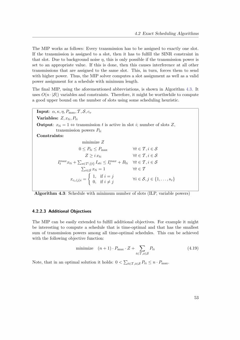
4.2 Exact Scheduling Algorithms
The MIP works as follows: Every transmission has to be assigned to exactly one slot.If the transmission is assigned to a slot, then it has to fulfill the SINR constraint inthat slot. Due to background noise η, this is only possible if the transmission power isset to an appropriate value. If this is done, then this causes interference at all othertransmissions that are assigned to the same slot. This, in turn, forces them to sendwith higher power. Thus, the MIP solver computes a slot assignment as well as a validpower assignment for a schedule with minimum length.
The final MIP, using the aforementioned abbreviations, is shown in Algorithm 4.3. Ituses O(n · |S|) variables and constraints. Therefore, it might be worthwhile to computea good upper bound on the number of slots using some scheduling heuristic.
Input: α, κ, η, Pmax, T ,S, cvVariables: Z, xti, PtiOutput: xti = 1⇔ transmission t is active in slot i; number of slots Z,
transmission powers PtiConstraints:
minimize Z0 ≤ Pti ≤ Pmax ∀t ∈ T , i ∈ S
Z ≥ i xti ∀t ∈ T , i ∈ SImaxt xti +
∑s∈T \t Isti ≤ Imaxt +Bti ∀t ∈ T , i ∈ S∑i∈S xti = 1 ∀t ∈ T
xcv(j)i =
1, if i = j0, if i 6= j
∀i ∈ S, j ∈ 1, . . . , sv
Algorithm 4.3: Schedule with minimum number of slots (ILP, variable powers)
4.2.2.3 Additional Objectives
The MIP can be easily extended to fulfill additional objectives. For example it mightbe interesting to compute a schedule that is time-optimal and that has the smallestsum of transmission powers among all time-optimal schedules. This can be achievedwith the following objective function:
minimize (n+ 1) · Pmax · Z +∑
t∈T ,i∈SPti (4.19)
Note, that in an optimal solution it holds: 0 <∑t∈T ,i∈S Pti ≤ n · Pmax.
53
4 Scheduling
4.3 Scheduling Heuristics
In the following, we will describe two heuristics for the scheduling problem. Theycan, for example, be used to achieve good solutions for big instances of the schedulingproblem, for an upper bound on the necessary number of slots, or for fast computationof good initial solutions for the ILPs. Section 4.3.1 deals with scheduling with fixedtransmission powers, Section 4.3.2 explores the problem with variable powers. In theremainder of this chapter, let T denote the set of transmission requests and n = |T |.
4.3.1 Fixed Transmission Power: MaxSINR
The main idea of the heuristic consists in processing one time slot after another andtrying to fill each slot with as many not yet scheduled transmissions as possible. Thisway, transmissions that are put together in a slot usually fit together very well, meaningthat they do not interfere too much with each other. In my student research paper [46],it is shown that one can achieve a good slot utilization by starting with an emptytransmission set A and consecutively adding the transmission t that maximizes theminimum SINR which occurs if all transmissions in A ∪ t are executed at the sametime.
Note, that the minimum SINR of all transmissions in A is strictly monotonically de-creasing with growing A. This means, if at some point the addition of a transmissiont ∈ T to the set of active transmissions A would result in a SINR γ < κ, it surely wouldalso lead to a signal-noise-ratio less than κ in every further pass of the loop. Thus,as soon as the addition of a transmission t to A leads to a SINR less than κ, we canremove it from the set T of possible transmissions. This substantially improves theperformance of the method.
This approach to fill a time slot efficiently is outlined in Algorithm 4.4. It uses a functionMinimumSINR which, given a set A of concurrently active transmissions, computes theminimum occurring SINR of all transmissions in A. In every step of the outer loop,at least one transmission is removed from T . Therefore, the outer loop is executednot more than O(n) times. The inner loop is executed O(n) times as well. If weimplemented MinimumSINR naively, then it had a running time of O(n2). This can beimproved to O(n), by storing for each transmission t ∈ A the interference at the receiverof t, caused by all transmissions in A. If we add a transmission, then this informationcan be updated in O(n) and the transmission with minimum SINR can, based on thisdata, also be determined in O(n). All together we get a running time of O(n3).
Now that we know how to fill a single slot efficiently, we just have to fill one slot afteranother until there are no transmissions left to schedule. This approach is outlined inAlgorithm 4.5. At this, FillSlot is the method described above.
54

4.3 Scheduling Heuristics
Input: Set T of transmissions, required signal-noise-ratio κOutput: Set A of concurrently feasible transmissionsA ← ∅maxMinSinr ← −1bestT ← undefinedwhile T 6= ∅ do
forall t ∈ T dosinr ← MinimumSINR(A ∪t)if sinr > maxMinSinr then
maxMinSinr ← sinrbestT ← t
if sinr < κ thenT ← T \ t
if maxMinSinr ≥ κ thenA ← A ∪ bestTT ← T \ bestT
elseT ← ∅
Algorithm 4.4: Good utilization of a time slot (fixed transmission powers)
Input: Set T of transmissionsOutput: Schedule S = (S1, S2, ..., Sn) such that S is a partition of Ti← 0while T 6= ∅ doSi ← FillSlot(T )T ← T \Sii← i+1
Algorithm 4.5: Computation of a good schedule
55
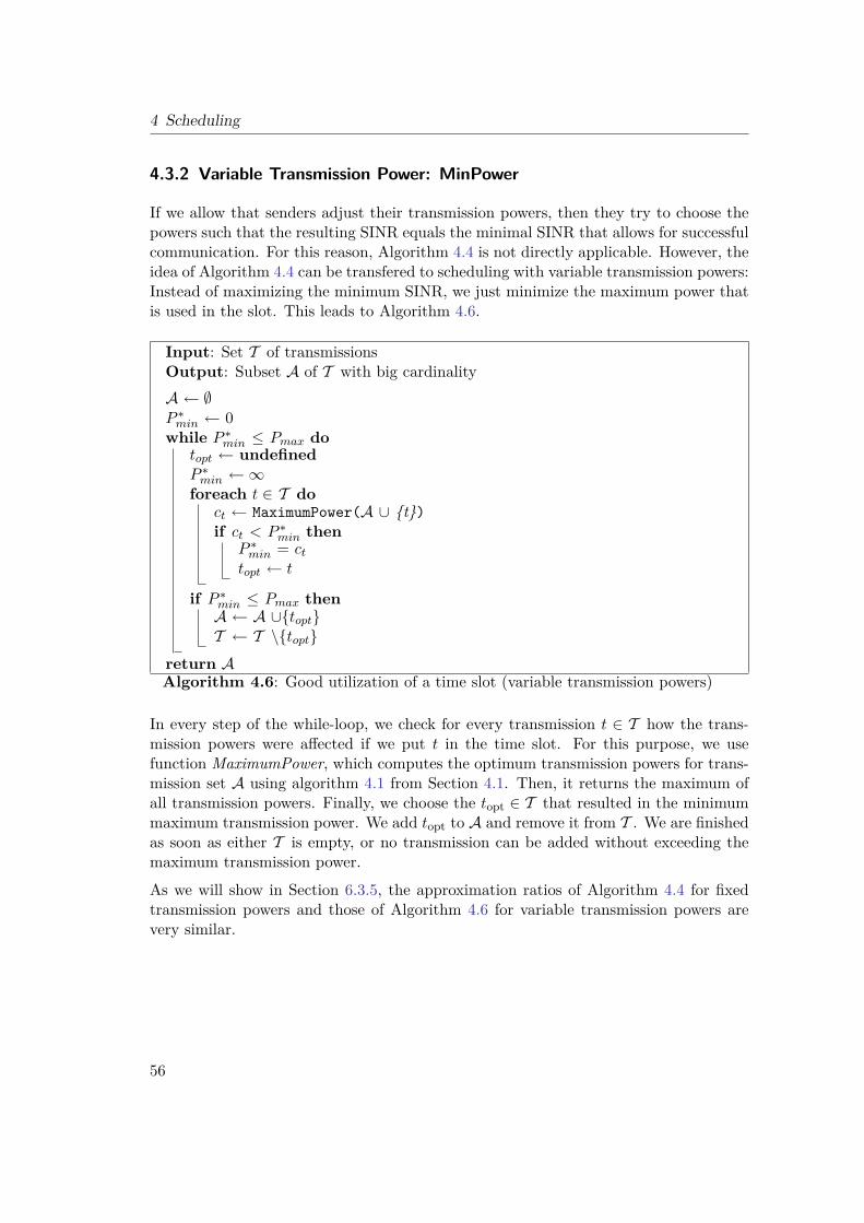
4 Scheduling
4.3.2 Variable Transmission Power: MinPower
If we allow that senders adjust their transmission powers, then they try to choose thepowers such that the resulting SINR equals the minimal SINR that allows for successfulcommunication. For this reason, Algorithm 4.4 is not directly applicable. However, theidea of Algorithm 4.4 can be transfered to scheduling with variable transmission powers:Instead of maximizing the minimum SINR, we just minimize the maximum power thatis used in the slot. This leads to Algorithm 4.6.
Input: Set T of transmissionsOutput: Subset A of T with big cardinalityA ← ∅P ∗min ← 0while P ∗min ≤ Pmax do
topt ← undefinedP ∗min ←∞foreach t ∈ T do
ct ← MaximumPower(A ∪ t)if ct < P ∗min then
P ∗min = cttopt ← t
if P ∗min ≤ Pmax thenA ← A ∪toptT ← T \topt
return AAlgorithm 4.6: Good utilization of a time slot (variable transmission powers)
In every step of the while-loop, we check for every transmission t ∈ T how the trans-mission powers were affected if we put t in the time slot. For this purpose, we usefunction MaximumPower, which computes the optimum transmission powers for trans-mission set A using algorithm 4.1 from Section 4.1. Then, it returns the maximum ofall transmission powers. Finally, we choose the topt ∈ T that resulted in the minimummaximum transmission power. We add topt to A and remove it from T . We are finishedas soon as either T is empty, or no transmission can be added without exceeding themaximum transmission power.
As we will show in Section 6.3.5, the approximation ratios of Algorithm 4.4 for fixedtransmission powers and those of Algorithm 4.6 for variable transmission powers arevery similar.
56

4.4 Computation of Lower Bounds for Optimum Schedules
4.4 Computation of Lower Bounds for Optimum Schedules
In this section, we will discuss methods for the computation of lower bounds for op-timum schedules. Lower bounds have several useful applications. For example, theycan be used to classify the quality of scheduling heuristics. Moreover, in cases where agood solution is sufficient, the lower bound can help to decide if a computed solutionalready fulfills the requirements. Sometimes, the lower bound equals the length of anoptimum schedule. Then, if we find a schedule whose length equals the lower bound,we immediately know that we are done and do not have to prove optimality or look forbetter solutions.
Conflict Graph Cliques
By definition, pairs of transmissions that are connected by an edge in the conflict graphcannot be scheduled concurrently. For this reason, the size of a set of transmissionsthat are all pairwise connected in the conflict graph gives a lower bound on the numberof slots of every valid schedule. Such a set of transmission forms a clique in the conflictgraph. As we are interested in good bounds, the maximum clique seems to be the toolof choice. We already utilized the maximum conflict graph clique to speed up the CPsand ILPs in Section 4.2. In this section, we will have a closer look on the properties ofconflict graph cliques.
Figure 4.1 shows a unit disk graph of 200 nodes which are distributed on an area of8 × 8 maximum transmission radii. The UDG has 859 edges that represent possiblecommunication links. In order to examine communications in such a topology, let usreplace every link of UDG by two transmission requests, one in each direction. Bydoing this, we model that every node wants to send one message to every other nodewithin transmission range. The conflict graph of the resulting transmission set consistsof 1718 nodes, one for every transmission. If a pair of transmissions cannot be scheduledsimultaneously, then they are connected by an edge in the conflict graph. We computedbig cliques in the conflict graph and highlighted the involved transmission red in theUDG.
It is striking that all transmission of the clique lie within the same area. This is notsurprising, as the interference caused by a sender falls of at least quadratically withdistance. However, this locality is extremely important for the feasibility of maximumclique computations. It is well known that the problem of computing a maximum cliqueis NP-complete. Usually, this means that the running time grows exponentially withproblem size. For sufficiently widespread networks, this does not hold in our case. Inmost realistic networks, nodes are placed apart from each other, to cover an area as bigas possible with as few as possible nodes. This restricts the density of nodes per area.Thus, the maximum number of edges incident to any transmission in the conflict graphis bounded by some constant b. This also means that no clique can have size greater
57

4 Scheduling
(a) Clique of SINR conflict graph (fixed power) (b) Clique of SINR conflict graph (variable power)
Figure 4.1: Unit disk graphs with maximum conflict graph cliques
than b. As soon as we decide to take one node to our clique, the size of the remainingproblem is reduced to O(b). Thus, every of the O(n) subproblems can be solved in timeO(2b). As b is usually rather big, this still might be intractable. Nonetheless, if weconsider b to be constant, the time complexity for finding a maximum clique is in O(n)for sufficiently large networks.
Our implementation of the maximum clique computation was able to find maximumcliques up to size 30-35 within reasonable time. In contrast to node density, the sizeof the network only played a minor role for the computation time. Unfortunately, fornetworks with densities like the network in Figure 4.1, this is not sufficient. The leftpicture shows a clique of the SINR conflict graph (fixed power), the right picture a cliqueof the SINR conflict graph (variable power). They consist of 133 transmissions and 116transmissions, respectively. Thus, at least with our implementation, this network is outof reach for computation of a maximum clique.
In such cases, when a maximum clique cannot be computed in reasonable time, onecan use heuristics to compute big cliques. One simple, yet efficient, heuristic is asfollows: Of all nodes in the conflict graph, choose one with maximum degree. If severalnodes have the same degree, choose the one whose corresponding transmission has thesmallest sender-receiver-distance. In the following, we maintain a list of candidates forour clique. This list is initialized with the neighbors of our selected node. For everynode n in the list of candidates, we compute the intersection of the list of neighbors ofn and the list of clique candidates. Now, among all nodes in the list of candidates, wechoose the one that had the most neighbors in the list of candidates. Again, in case
58

4.4 Computation of Lower Bounds for Optimum Schedules
of a tie, we select the node with smaller sender-receiver-distance. The selected node isremoved from the list of candidates and added to our clique. Furthermore, all nodesthat are not neighbors of the selected node are removed from the list of candidates.This process is repeated until the list of candidates is empty. In our tests, this simpleheuristic performed very well. The cliques in Figure 4.1 also have been computed usingthis heuristic.
Chromatic Number of the Conflict Graph
The chromatic number of a graph G is the smallest number of colors needed to colorthe vertices of G such that no two adjacent vertices share the same color. Given such acoloring of the vertices of our conflict graph, we can assign all transmissions with samecolor to the same time slot. This gives us a schedule in which all transmissions cantransmit pairwise simultaneously. The chromatic number of a graph must be greaterthan or equal to the size of a maximum clique. Therefore, the chromatic number pro-vides a better lower bound than the maximum clique. Yet, this slight improvement canonly be achieved with tremendous additional computational effort. Like the maximumclique problem, the computation of chromatic numbers is NP-complete [40]. Moreover,the locality that helps to speed up the computation of maximum cliques does not existfor the computation of chromatic numbers. As we will see in Section 6.3.5, the lowerbound provided by the maximum clique is already almost optimal. For this reason, wedo not consider the computation of the chromatic number of the conflict graph being agood lower bound heuristic.
LP relaxation of the ILPs and MIPs
For every ILP or MIP, one can replace the requirement that variables are integer by ap-propriate continuous constraints. Objective function and constraints are not modified.The resulting problem is called the LP relaxation [1] of the original problem. Now thatwe have only continuous variables, the LP relaxation can be solved in polynomial timeusing an LP solver. Thus, the LP relaxation usually can be solved for very big probleminstances. In general, the solution values of the relaxed problem are not integer. But inmany problems, they can be rounded to a feasible solution of the integer program. Theobjective value of an optimum solution of the relaxed problem gives a lower (upper)bound on the optimum solution of the original minimization (maximization) problem.
To evaluate the quality of this lower bound, we solved the LP relaxation for differentformulations of the scheduling problem. Unfortunately, the results were very poor. Inthe LP relaxation, it is allowed that transmissions are not completely scheduled in a slot,but only fractions of them. What happened was, that all transmissions were distributedover several slots. As a result, the interferences were much lower and the value of the
59

4 Scheduling
objective function was not a good approximation on the length of an optimal scheduleof the original problem.
60

5 Topology Control
Most of the topology control algorithms proposed recently are local. This means, thatevery node of the network only has to know his own neighborhood in order to decidewhich links he wants to keep and which links he wants to discard. In realistic scenarios,this locality is a useful property for algorithms used in sensor networks. Especiallyin ad-hoc networks, nodes usually only know their neighborhood, and it would be tooexpensive to maintain positions of all involved nodes.
Yet, there are some useful applications for centralized algorithms. For example, if theconsidered network is static, it can be worthwhile to have a one-time negotiation phasein the beginning, in which all nodes agree on a global schedule. Every link of thetopology is assigned to a time slot such that a collision-free transmission is guaranteed.This schedule is repeated perpetual. Especially in networks where the nodes only haveto communicate infrequently, and where power-awareness is of special importance, sucha TDMA approach (cf. Section 3.2) might be interesting. Of course, the length of theschedule strongly influences the network performance and latency. Therefore, methodsthat compute topologies that can be scheduled in a minimal number of slots are of highinterest.
In this chapter, we describe two algorithms that compute topologies with the goal ofminimizing the number of slots necessary to schedule all topology links. One of them isbased on the scheduling heuristics from the last chapter, the other one uses an approachsimilar to the LIFE algorithm (cf. chapter 5.1.2), but using another interference measurethat is motivated by the SINR model. Both algorithms can be used to find connectedtopologies, as well as topologies which are spanners of certain graph properties.
In order to classify the quality of the produced topologies, we will compare them toa number of existing topology control algorithms in the experimental section. Thosealgorithms are described in Section 5.1.
We conclude this chapter with a description of a CP that computes topologies whoselinks can be scheduled using minimum number of slots.
5.1 Overview of existing Algorithms and Topologies
Additional to the topology control algorithms that we will describe later, we imple-mented several existing algorithms and compared them to our algorithms and to each
61

5 Topology Control
other. These algorithms, as well as some other famous topology control algorithms, aredescribed in the following. Example topologies of most of the described algorithms canbe found in the experimental chapter.
5.1.1 Gabriel Graph and Relative Neighborhood Graph
As stated before, local algorithms are of special importance in the field of wirelessnetworks because they allow for a distributed computation and thus help to avoidnetwork traffic and to save energy. Therefore, it is not surprising that well-knownlocally definable graphs have been among the first proposals for topology control. Twofamous examples are Gabriel graphs and relative neighborhood graphs.
In a Gabriel graph, a pair of vertices is only be connected by an edge, if the diskwith the vertices as diameter contains no further vertices. This situation is depictedin figure 5.1(a). The area that is shaded gray has to be empty. In our special case ofnetwork topologies, the nodes furthermore have to be within transmission range to beconnected.
(a) Gabriel Graph (b) Relative Neighborhood Graph
Figure 5.1: Edges in Gabriel graphs and relative neighborhood graphs
In a relative neighborhood graph, two vertices can only be connected by an edge if theintersection of the two disks centered at the endpoints of the edge, with their radii equalto the distance between the two vertices, is empty. This area is highlighted in gray infigure 5.1(b). Again, in the case of network topologies, an edge is not allowed to exceedthe maximum transmission radius.
If a node knows its neighborhood, then it can easily decide for all possible links ifthey belong to the Gabriel graph or to the relative neighborhood graph. Thus, thosetopologies can be computed extremely efficient in a distributed fashion.
Both, Gabriel graph and relative neighborhood graph are known to be connected, planarand sparse. Further information on relative neighborhood graphs and their relativescan be found in [16].
62

5.1 Overview of existing Algorithms and Topologies
5.1.2 LIFE and LISE
In [3], Burkhart et al. examine the question if so-far proposed topology control algo-rithms really help to reduce interference. They show that neither sparseness nor lownode degree are guarantees for low interference. Furthermore, they precisely definetheir notion of interference. This definition of interference is based on the question,how many nodes are affected by communication over a certain link. Given a networkG = (V,E) and a transmission (u, v) ∈ E from sender u ∈ V to receiver v ∈ V , theydefine D(u, r) to be the disk centered at u with radius r = dist(u, v). If u sends to v, ac-cording to their definition, all nodes within the disk D(u, r) are affected. Additionally,they define the coverage Cov(u, v) of an edge (u, v) as the number of network nodesthat are affected, if nodes u and v communicate with each other. At this, it is assumedthat u and v choose their respective transmission powers such, that they exactly reacheach other. Formally:
Cov(e) := |w ∈ V |D(u, |u, v|) coversw| ∪ |w ∈ V |D(v, |v, u|) coversw|
Based on this interference measure, they further introduce two scheduling algorithms.
Low Interference Forest Establisher (LIFE) LIFE is a global algorithm which findsa connectivity-maintaining, interference-optimal topology G′ = (V,E′), meaningthat the connectivity is preserved and the maximum coverage Cov∗(E′) of alledges e ∈ E′ is minimized. The algorithm works similar to Kruskal’s minimumspanning forest algorithm, using the coverage of the links as edge weights.
Low Interference Spanner Establisher (LISE) In contrast to LIFE, LISE establishes atopology that is a distance-spanner. With slight modifications, the algorithm canalso be used to compute a hop-spanner topology. First, the algorithm computes alink with minimum coverage Covmin. Then, it adds all links with coverage Covminto the topology. If the desired spanner-property is fulfilled, the algorithm stops.If not, it again determines an edge with minimum coverage Covmin among theremaining edges and adds all edges with coverage Covmin to the topology. Thisis repeated until the desired spanner-property is satisfied. Again, the topology isinterference-optimal, meaning that the maximum interference among all edges ofthe topology is minimized. Furthermore, in order to compute a t-spanner, everynode only has to know its ( t2)-neighborhood. Thus, the algorithm is local.
5.1.3 Minimum Spanning Tree Algorithms
There exist several algorithms, which, like the LIFE algorithm, define some weight onthe edges and subsequently compute a minimum spanning tree of the weighted graph.Probably the most famous of them is the Euclidean minimum spanning tree (EMST),
63

5 Topology Control
which uses the Euclidean distance as edge weights. The EMST topology can also beused to bound the maximum node degree, as every EMST of a finite set of points inthe plane has a maximum node degree of six [29].
5.1.4 Cone Based Topology Control (CBTC)
The basic idea of the CBTC algorithm is that every node u transmits with the mini-mum power pu,α required to ensure that in every cone of degree α around u, there issome node that u can reach with power pu,α. In [24, 25], Li et al. show that usingα = 5π/6 is a necessary and also a sufficient condition to guarantee that network con-nectivity is preserved. Besides, they propose three optimizations that further reducepower consumption and prove that they retain network connectivity.
A node u is said to be a boundary node if u has still an α-gap at the end of the algorithm.In the basic CBTC(α) algorithm, all boundary nodes would broadcast with maximumpower. The Shrink-Back Optimization reduces the transmission powers of all boundarynodes as much as possible without reducing the cone coverage of the nodes.
Let Eα be the set of edges of the topology Gα = (V,Eα) computed by the CBTC(α)algorithm. The second optimization, the Asymmetric Edge Removal, removes all di-rected edges (u, v) ∈ Eα from the topology Gα for which (v, u) 6∈ Eα. Li et al. provethat this optimization preserves connectivity for α ≤ 2π/3.
The so called Pairwise Edge Removal is the third and last optimization proposed in [25].They show that, for α ≤ 5π/6, if there is an edge from u to v and from u to w, then thelonger edge is redundant and can be removed as long as d(v, w) < max(d(u, v), d(u,w)).Since the transmission power of each node should be reduced, only the redundant edgeswith length greater than the longest non-redundant edge are removed.
One of the advantages of their algorithm is that it does not need the exact positionsof the sensor nodes but only directional information. According to the authors, CBTCwas the first algorithm that simultaneously achieved a variety of useful properties, suchas symmetry, sparseness, and good routes [25].
5.1.5 XTC Algorithm
The XTC algorithms was proposed by Wattenhofer et al. in [48]. Compared to mostpreviously proposed algorithms, it is really simple: Two vertices u and v are connectedif they are within transmission range and if there is no vertex w which is closer toeither u or v than u and v are to each other. XTC is strictly local and does not requireavailability of node position information. Besides, the underlying network graph doesnot need to be a Unit Disk Graph. Instead, XTC works on every general weightednetwork graph.
For the special case that the network graph is a Unit Disk Graph, the resulting topology
64

5.2 Topologies which can be efficiently scheduled
has bounded degree, is a planar graph, and—on average-case graphs—a good span-ner [48].
5.2 Topologies which can be efficiently scheduled
In the following sections, we study the problem of computing time-optimal topologies.We define a time-optimal topology as follows:
Definition 5.1 (Time-optimal topology). Given an input graph G = (V,E) and somegraph property Ψ, a topology G′ = (V,E′), E′ ⊆ E, is a time-optimal topology ofG regarding Ψ, if it fulfills Ψ and if there does not exist another topology G∗(V,E∗),E∗ ⊆ E, which also fulfills Ψ and whose edges can be scheduled with less time slotsthan the minimum number of slots required to schedule all edges of G′.
At this, every edge u, v of a topology is regarded as two transmissions (u, v) and(v, u), one in each direction. In the following, we require that the considered graphproperty Ψ is either preservation of connectivity, or some spanner-property, such ashop-spanner, distance-spanner, or power-spanner. The proposed methods cannot beused with arbitrary properties. In this case, preservation of connectivity means thateach pair of nodes that is connected by a path in G also has to be connected by a pathin G′.
5.2.1 MaxSINR Topology and MinPower Topology
In our experiments, the scheduling heuristics from Section 4.3 produced very goodschedules. Therefore, it is tempting to extend them to topology control algorithms,hoping that the links of the resulting topologies can also be scheduled efficiently. Thebasic idea of both scheduling algorithms was to fill the slots one by one, as good aspossible. Every slot is filled in a greedy fashion, such that the minimum SINR ismaximized, or that the necessary maximum power is minimized. These approaches canbe extended to topology control algorithms as follows: We still add the transmissionsone by one to the schedule. Furthermore, we maintain a data structure, which allows tocheck efficiently if a transmission t is still necessary to fulfill the required graph propertyΨ. As soon as we encounter a transmission that is no longer necessary, we remove itfrom the list of unprocessed transmissions. In the end, all transmission that have beenassigned to slots belong to the topology.
If we want the topology to be undirected, we have to take care that for every trans-mission that has been scheduled, the second transmission belonging to the same edge(in opposite direction) also will be scheduled. For this purpose, we add a marker toeach transmission. As soon as one of the transmissions belonging to an edge is addedto the topology, we mark the second transmission of the edge as necessary. Thus, the
65
5 Topology Control
transmission will be scheduled for sure at some point. Besides, as soon as we add thefirst transmission t1 = (u, v) of a pair (t1, t2) of transmissions to some slot, we updateour data structure as if t2 = (v, u) already belongs to the topology.
Let us see how we can maintain the aforementioned data structure and how we candecide if a transmission is unnecessary:
Connectivity If m is the number of nodes in the network, we just need a m×m-matrixC, which stores for every pair of nodes whether it is already connected. Everytime a transmission (u, v) is added, we check for all nodes if they are alreadyconnected by some path to u and not yet connected to v. For all nodes that fulfillthis requirement, we update the connectivity information in C such that they noware also connected to v, as well as to all nodes that are reachable from v.If we have to decide if a transmission t = (u, v) should be added to the topology,we check using C[u, v] if they are already connected by some path. If this is trueand t is not marked to be necessary, we know that we can discard t.
It is obvious, that in the end all pairs of nodes that are in the same connected componentof the input graph are also connected by some path in the resulting topology. This holds,because no edge which could be used to connect two yet unconnected components inthe new topology is discarded.
Spanner-Property Given some distance measureM, we compute for all pairs (u, v) ofnodes the length p(u, v) of a shortest path in the weighted input graph G = (V,E).If we want to compute a s-spanner G′ = (V,E′) with regard to M, we have tomake sure that the length p′(u, v) of a shortest path between every pair (u, v) ofnodes in G′ is at most s times the length p(u, v). In the beginning, all distancesin G′ are set to∞. Every time we add a transmission t = (u, v) with edge-weightw(u, v), we check for all nodes x ∈ V if p′(x, u) + w(u, v) < p′(x, v). For allnodes which fulfill this condition, we update all shortest path lengths p′(x, z) top′(x, z) = minp′(x, z), p′(x, u) + w(u, v) + p′(v, z).If we have to decide if a transmission t = (u, v) should be added to the topology,we check if p′(u, v) ≤ s ·p(u, v). If this is true, we know that there already exists apath between u and v that fulfills the s-spanner property, and, if t is not markedas necessary, we can discard it.
In the end, every node u is connected in G′ to all of its neighbors v in G by a pathp′(u, v) with p′(u, v) ≤ s · w(u, v).
Then, for all u, v ∈ V , it holds that p′(u, v) ≤ s · p(u, v). Proof: Let (u, x1, . . . , xn, v) bea shortest path between u and v in G. Every edge (v1, v2) of this path can be replacedin G′ by a path with length less than or equal to s · w(v1, v2). Thus, there exists apath in G′ that is not longer than s · p(u, v) and G′ is an s-spanner with respect to thedistance measure.
66

5.2 Topologies which can be efficiently scheduled
Note, that these algorithms are not proposed to be used in real networks. They aremainly intended to verify if topologies that are generated by such an approach are easierto schedule than topologies which are produced by simpler heuristics. We will see later,that the produced topologies can be scheduled very well, but that the much easierapproach to greedily take the shortest links into the topology generates topologies thatare equally good.
5.2.2 MinInterference Topology
Many of the existing topology algorithms try to minimize some interference measure.The proposed interference measures range from node degrees to the coverage of an edgethat was used for the LIFE and LISE algorithms (cf. Section 5.1.2).
To our knowledge, there exists no interference measure for topology edges that is mo-tivated by the SINR model. Such an interference measure has to take into accountthat transmissions over shorter distances can tolerate more interference and that theinterference received from some sender decreases with the distance with path loss expo-nent α. Furthermore, if the measure should be meaningful, there has to be some upperbound on the interference received from a single sender. This is because the worst thingthat can happen is that a pair of transmissions cannot be scheduled concurrently. Ifthis is the case, it does not matter how close together interfering sender an disturbedreceiver actually are.
Therefore, we define that the interference I(t1, t2) from transmission t1 to anothertransmission t2 equals 1 if t1 and t2 cannot be active simultaneously. For a pair oftransmissions (t1, t2) that can be scheduled together, we define I(t1, t2) as follows: LetB(t2) be the maximum interference that t2 can tolerate if the sender of t2 sends withmaximum power, and let I(t1, t2) be the interference that transmission t1 causes at t2in the case that the sender of t1 sends with maximum power. Now, for our interferencemeasure, we define the interference I(t1, t2) from t1 to t2 as I(t1, t2) = I(t1, t2)/B(t2).This equals the fraction that t1 uses of the interference buffer of t2 if both transmitwith maximum power.
Then, the interference I(t) of a transmission t is the sum of the interferences from alltransmissions that interfere with t. The interference I(e) of a topology edge e = u, vis defined as the sum of the interferences of transmissions t1 = (u, v) and t2 = (v, u)that represent e in our optimization problem.
The proposed topology control algorithm is now similar to the LIFE algorithm, withthe difference that we use our interference measure I(e) instead of coverage Cov(e).In order to be able to compute spanner topologies, we further use the techniques fromSection 5.2.1. It is shown in [3], that it is sufficient to consider the t-neighborhood ofevery node to compute a topology that is a t-spanner based on an appropriate distance
67

5 Topology Control
measure. Thus, if we compute a spanner instead of a spanning tree, the algorithm canbe realized based on local information.
Our interference measure I(e) has several advantages compared to Cov(e): Both, theinterference buffer B(t) of a transmission and the interferences I(t1, t2) can be deter-mined without having any knowledge about positions, distances, or directions. In aninitial phase, the nodes just have to send ping messages with maximum power to al-low the other nodes to measure the received signal strength. Then, the nodes tell theother nodes which signal strengths they measured. There is nothing more necessaryto compute the required information. This approach even takes into account obstaclesthat negatively influence the power gain between pairs of nodes. Furthermore, it isconsidered that transmissions over short ranges can tolerate more interference.
Note, however, that we build our topology based on the interferences weights thatevery node gets assigned in the input graph. In general, the final topology has muchless edges. Thus, the interference measure of an edge differs between input graphand output topology. The resulting topology therefore is not optimal regarding ourinterference measure. Nevertheless, it seems to be a good heuristic and this topologycontrol algorithm performed very well in our experiments. It should be especially usefulin situations where no kind of position information is available, or when the signalstrength is not solely determined by distance.
5.2.3 Constraint Programming
The constraint programs from Section 4.2.1 can be extended to a CP formulation thatfinds, given an input graph G = (V,E), a time-optimal topology fulfilling the desiredgraph property Ψ. For this, we introduce for every edge e = u, vof the input graph twotransmissions t1 = (u, v) and t2 = (v, u), which have to be scheduled. In the following,let m = |V | be the number of nodes, and n = 2|E| the number of transmissions.
To be able to model that some edges do not belong to the resulting topology, weintroduce a new dummy time slot with ID 0. The transmissions corresponding to edgesthat do not belong to the final topology are assigned to this dummy time slot.
Let us first assume that we want to preserve connectivity in our resulting topology. Weintroduce m2 new Boolean variables connected[u][v], which store for every pair (u, v)of nodes, whether they are already connected in the current partial topology. If atransmission t = (u, v) is added to the partial topology, then its sender and receiver areconnected. This can be realized by a constraint
slot[t] > 0⇒ connected[u][v] = 1 (5.1)
for all transmissions (u, v) ∈ T . For every triple (u, v, w) of nodes, we add anotherconstraint
connected[u][v] ∧ connected[v][w]⇒ connected[u][w] (5.2)
68

5.2 Topologies which can be efficiently scheduled
Now, every time a transmission t is added, Gecode updates the connectivity variablesin O(n2).
To achieve that transmissions are not taken into the topology, if they are not neces-sary because sender and receiver are already connected otherwise, we add, for everytransmission t = (u, v), a new custom propagator to connected[u][v], which enforces:
connected[u][v] = 1 ∧ slot[t] is not yet assigned⇒ slot[t] = 0 (5.3)
Next, as we want to get an undirected topology, we add for each edge u, v ∈ E withcorresponding transmissions t1 = (u, v) and t2 = (v, u) a constraint:
slot[t1 ] > 0⇔ slot[t2 ] > 0 (5.4)
Now, let us get to the branching: As we do not have to schedule all transmissions,it does no longer seem to be a wise choice to always select the transmission variablewith minimum domain size for the next branching. If we would do so, we would firstcheck out the variables that suffer from the most interference. There is a good chance,that these variables do not belong to an optimum topology. Instead, we order thetransmissions according to their sender-receiver-distance, and begin with the short-distance transmissions. As we will see later in the experimental section, good topologiesusually mainly consist of the shortest edges of the input graph. Now, the order in whichthe values from the domain of the chosen variable are checked out has to be determined.Again, it seems to be a good choice to start with the slots in which the consideredtransmission receives least interference. If we unsuccessfully tested out all possibilitiesto assign the transmission to one of the slots, we assign it to the dummy slot 0, meaningthat the corresponding edge will not be in the final topology. Thanks to constraint 5.4,the second transmission belonging to the same edge will automatically be assigned toslot 0.
Every solution of the CP that is found defines a spanning forest of the input graph. Assoon as we find a new solution, we add a new constraint that enforces that the nextsolution has to be scheduled using one slot less.
This CP can be easily adjusted to compute topologies which fulfill arbitrary graphproperties. Let us, for example, assume that we want to compute a topology that is adistance s-spanner. To do this, we maintain a matrix of shortest paths in the partialsolution and implement a new propagator, which keeps this matrix up to date. As weare only interested in a distance s-spanner, it is sufficient to consider the s-neighborhood(meaning the neighborhood within a radius of s times the maximum transmission range)of every node. If for every node the distance stretch factor to every other node in thes-neighborhood is below s, then the stretch factor to all nodes in the topology is belows [3]. Now, the decision whether a transmission has to be scheduled or not is madedirectly within the branching. If the nodes involved in a transmission t are alreadyconnected with stretch factor less than s in the current topology, then t is unnecessary
69

5 Topology Control
and we can immediately set slot[t] = 0. If the nodes are not yet connected, or if they areconnected only with stretch factor greater than s, we first try to assign the transmissionto any of the possible slots before we decide to discard it from our topology.
Note that the maximum clique optimization cannot be used in connection with thisCP formulation, as we cannot be sure that all transmissions of a maximum clique dobelong to edges of a time-optimal topology. We first expected that the CP that onlypreserves connectivity should be usable in networks with many edges, because we neverhave to schedule more transmissions at the same time than twice the number of nodes.Unfortunately, if we want to prove optimality, this assumption is wrong. The reason forthis is, that, given 2|E| transmissions, the number of valid partial schedules is immense,even if not all transmissions have to be scheduled at the same time.
70
6 Experimental Results
Most of the algorithms and techniques described in this thesis have been implementedin Java and C++. In this chapter, we use these implementations to analyze somefundamental properties of sensor networks and to compare the performance and runningtimes of the different methods. At this, the comparison between the constraint programsand the integer programs is one of the main aspects.
This chapter is organized as follows: In Section 6.1, the implementation and testingenvironment are specified. Afterwards, in Section 6.2, we show important aspects ofthe choice of SINR model parameters and describe which parameters were used for theexperiments in this thesis. The experiments that are related to scheduling can be foundin Section 6.3, those related to topology control in Section 6.4.
6.1 Implementation and Testing Environment
The algorithms and methods which are described in this thesis have been implementedpartly in Java and partly in C++. For the solution of the ILPs and CPs, we used theexternal solvers ILOG CPLEX 11 [5] and Gecode 2.1.1 [7]. CPLEX is a commercialproduct and is known to be one of the fastest and most developed solvers for (integer)linear programs. Gecode is an open source environment for modeling and solution ofconstraint programs. A detailed introduction into Gecode is given in Section 2.4.
Originally, we intended to do all the implementations in Java, in order to avoid im-plementing the core functionality (e.g., the SINR model) twice. We decided on Javabecause it is freely available, highly portable, almost as fast as C++, and there areseveral good libraries for the visualization of graphs and networks available.
Unfortunately, the Gecode libraries for Java are currently, according to the authors,mainly intended for testing purposes and not optimized for high performance. Normally,this is no problem as the performance of a constraint program is usually measured inthe number of failures and backtracks, and not in running time. The number of failuresallows for comparisons which are independent of the testing environment and the CPsolver in use. But as one of the goals of this thesis was to evaluate the usability ofconstraint programming compared to integer linear programming, it would have beenunfair to compare the actual running times of the Java Gecode implementation withthe running times of the highly optimized ILOG CPLEX Solver. For this reason, theconstraint programming related parts have been implemented in C++.
71
6 Experimental Results
For the visualization of the sensor networks, we used JUNG 2.0 alpha 1 [17], the JavaUniversal Network/Graph Framework.
The experiments and running time comparisons have been done on a computer withtwo Dual-Core AMD OpteronTM 2218 processors (2.6 GHz) and 32 GB RAM, runningLinux 2.6.16.13 (SUSE).
6.2 Parameters used for the SINR Model
In order to stay realistic, it is assumed that every sensor node has some maximumtransmission power Pmax. For the sake of simplicity, we use the same maximum trans-mission power for all sensor nodes. In the case of fixed transmission powers, we setP = Pmax. The minimum SINR κ is set to 10, a value which should be realistic formodern hardware. For the path loss exponent we choose α = 4 .
If we consider the case that there is no interference due to concurrent transmissions andsolve the SINR inequality for the distance d between sender and receiver, this gives us:
d ≤ α
√Pmaxηκ
(6.1)
As α, η, and κ are constants, it is obvious that the maximum transmission powerimplies a maximum transmission range dmax. In order to make the results descriptivefor the reader it seems to be natural to normalize the parameters by setting η such thatPmax = 1 and dmax = 1. This means η = κ−1.
However, this can lead to undesirable results. If we allowed transmissions over a distanceof almost one, then this would mean that the transmission cannot tolerate concurrenttransmissions even from senders relatively far away. This is unrealistic and complicatestheoretical considerations about the model. Therefore, it is better to restrict transmis-sions to a maximum sender-receiver-distance d∗max < dmax. In the following, we willrefer to d∗max as transmission radius. We can normalize d∗max to the value 1 using thefollowing definition for η:
η = 1(1 + β)κ (6.2)
In this equation, β is some arbitrary constant that defines how much interference (inmultiples of η) every transmission with transmission power Pmax and sender-receiver-distance less than or equal d∗max = 1 should be able to tolerate from concurrent trans-missions.
The advantage of using d∗max instead of dmax as maximum sender-receiver-distance isshown in Figure 6.1. The left picture shows 145 nodes which are randomly distributedin an area of 12 × 12 units of length. Every pair of nodes with distance not greaterthan 1 is connected. Now, we compare the conflict graphs in dependence of our choice
72

6.3 Scheduling
(a) Unit Disk Graph (b) Bad model parameters (c) Good model parameters
Figure 6.1: Good vs. bad choice of SINR model parameters
of β. The result for β = 0 can be seen in Figure 6.1(b): Even transmissions which arereally far away from each other conflict with each other. Theoretically, a transmissionover distance dmax could fail because of one single active sender in arbitrary distance.Figure 6.1(c) shows the situation for β = 1. Here, the conflicts only occur betweentransmissions whose nodes are near to each other as one would expect in reality.
6.3 Scheduling
In the following sections, we study several properties of wireless networks that arerelated to scheduling. After a brief description of our test data, we compare graph-based interference models with the SINR model. Subsequently, we examine optimumschedules and the advantages of using variable transmission powers instead of fixedtransmission powers. This is followed by an evaluation of the quality of our schedulingheuristics, as well as of the lower bounds that are achieved by computing a maximumclique of the conflict graph. The ILPs and CPs are compared based on the percent-age of problems which they were able to solve within 180 seconds, and based on theaverage number of slots of the schedules that they found within the given time. Thissection concludes with an evaluation of random restarts as a tool to speed up constraintprograms.
6.3.1 Test data
In order to make the different experiments as comparable as possible, most of theexperiments were run on the same sets of input data. The defining properties of eachdata set are the number of transmissions and the dimensions of the area on which thetransmissions are placed. Obviously, both play an important role for the running time of
73

6 Experimental Results
the algorithms as well as for the number of slots in an optimum solution. The dimensionsof the considered area are given in transmission radii. At this, a transmission radius isthe maximum distance between a sender and a receiver, such that they still are ableto communicate if the only interference is caused by the background noise η. The datasets are divided into three big classes, depending on the dimensions of the test area:5× 5 transmission radii, 10× 10 transmission radii, and 15× 15 transmission radii. Ofcourse, this only covers rather small sensor networks. But, due to the NP-hardness ofthe scheduling problem, the computation of exact solutions for bigger instances wouldbe too time-consuming. Nevertheless, the results show clear tendencies and thus canbe easily transfered to bigger dimensions.
For the classes with 5× 5, 10× 10, and 15× 15 transmission radii, we created data setswith n = 10, 20, ..., 100, n = 10, 20, ..., 120, and n = 10, 20, ..., 170 transmissions, respec-tively. Each data set consists of 50 random transmission sets. They were generatedby first placing each sender randomly within the test area and, afterwards, placing thecorresponding receiver randomly within transmission range such that the receiver alsolies in the test area.
(a) 5× 5 radii, 100 transmissions (b) 10 × 10 radii, 100 transmis-sions
(c) 15 × 15 radii, 100 transmis-sions
Figure 6.2: Examples of the transmission sets used for the scheduling experiments
Of course, the transmission density, meaning the number of transmissions per unitarea, is the main determination factor for the number of slots in an optimum schedule.Therefore, in order to give a first impression on the transmission densities, Figure 6.2depicts three of the overall 1950 transmission sets.
74
6.3 Scheduling
6.3.2 Graph-based Models vs. SINR Model
There are several scheduling algorithms that are based on conflict graphs. Depending onthe quality of the conflict graph used, these algorithms either put transmissions whichcannot be scheduled together into the same slot, or they do not allow the concurrentexecution of transmissions which actually could be scheduled together. It is widelybelieved that the SINR model represents reality pretty well. Therefore, it seems tobe interesting to compare some frequently used conflict graph models to the SINRconflict graph. Edges additional to the edges of the corresponding SINR conflict graphindicate that the considered model is over-restrictive, edges missing compared to theSINR conflict graph indicate that the model is not sufficiently restrictive.
The first experiment to compare graph based conflict graphs with the SINR conflictgraph is accomplished as follows: We generated 100 node sets of 300 nodes at a time,which have been randomly distributed within an area of 15×15 transmission radii. Foreach of the node sets, the unit disk graph was constructed. Then, we computed theconflict graphs of the following models:
Distance-2 Fixed Model In the distance-2-fixed model, every sender has a fixedtransmission range r. If two transmissions t1 = (u, v) and t2 = (u′, v′) are activeconcurrently, then transmission t1 fails if
dist(u′, v) ≤ r. (6.3)
Distance-2 Variable Model In the distance-2-variable model, every node adjusts itstransmission range on a per-message basis. Here, transmission t1 fails if
dist(u′, v) ≤ dist(u′, v′). (6.4)
Sigma Model In the σ-model with parameter σ ≥ 0, the distance between sender uand corresponding receiver v is taken into account. Furthermore, the parameterσ allows to specify, that the interference is not restricted to the maximum trans-mission range r. Transmission t1 = (u, v) fails, if for some concurrently activesender u′
dist(u′, v) ≤ (1 + σ)dist(u, v). (6.5)This model comes closest to the SINR model.
Two Hop Model In the two-hop model, two transmissions are interfering if thecorresponding edges in the unit disk graph are adjacent or if they are connectedby an edge. This model was used by Tamura et al. in [42].
The average edge numbers of the resulting conflict graphs now give some insight on howthe methods behave compared to the SINR conflict graphs. The results can be seen inTable 6.1. For the sigma model, σ = 2.16 was used.
75

6 Experimental Results
Distance-2 Fix Distance-2 Var Sigma Two HopConflict graph edges 12161.9 9127.1 20464.4 13854.7Additional to SINR Fixed 476.1 44.5 2664.2 808.4Missing from SINR Fixed 6114.4 8717.6 0.0 4753.9Additional to SINR Var 1717.7 401.5 7849.0 2508.9Missing from SINR Var 2171.2 3889.8 0.0 1269.6
Table 6.1: Number of edges in different conflict graph models
The SINR conflict graph (fixed power) and SINR conflict graph (variable power) hadan average of 17800 and 12615 edges, respectively. Again, it can be seen that the useof variable transmission powers pays off. The first thing that strikes if one looks atTable 6.1 is that all conflict graphs contain a big number of edges that do not existin the corresponding SINR conflict graph. The reason for this is, that the models donot take advantage of short distances between senders and corresponding receivers.As the signal quality decreases extremely fast with the distance, a short sender-receiverdistance means that the transmission can tolerate much interference from outside. How-ever, being too cautious with concurrent transmissions is by far not as bad as allowingtransmissions to be scheduled together which interfere so much that one or both trans-missions fail. Unfortunately, all models but the Sigma model are missing a tremendousnumber of edges from the SINR conflict graph. This certainly shows that schedulingbased on this conflict graphs does not result in reliable schedules.
So let us have a closer look on how the conflict graph models differ. Figure 6.3(a)shows a set of randomly distributed sensor nodes with corresponding unit disk graph.The vertices of the corresponding conflict graph are depicted in Figure 6.3(b). In theremaining pictures of Figure 6.3, the different conflict graphs are compared. Probablythe most obvious distinction is, that the SINR conflict graphs connect edges that donot belong to the same connected component.
If one wants to use a graph based model and tolerates rare cases of transmission failures,then the SINR based conflict graphs should be the first choice. On the other hand, iffailures are not tolerable, then the methods proposed in my student research paper [46]and in [20] should be considered.
6.3.3 Analysis of Optimum Schedules
In this section, we will have a closer look on the properties of optimum schedules.Figure 6.4 shows the average slot numbers of the schedules that were generated withthe ILPs and CPs described in this thesis. The scheduling problems have been solvedto optimality for most of the transmission sets. If neither the ILP nor the CP was ableto compute the optimum solution within the given time, then the best of both solutions
76

6.3 Scheduling
(a) Unit Disk Graph (88) (b) Conflict Graph Vertices (c) SINR Fixed (5142)
(d) SINR Variable (3612) (e) Distance-2 Fixed (1302) (f) Distance-2 Variable (1050)
(g) Sigma 2.16 (2554) (h) Two-Hop (1516)
Figure 6.3: Graph-based conflict graphs vs. SINR-based conflict graphs
77

6 Experimental Results
was used. More information on the transmission sets which could not be solved tooptimality and the quality of the resulting schedules can be found in Section 6.3.6. Byall means, we can assume that the schedules which we analyze in this chapter are almostoptimal if not optimal. At this point, we only want to analyze the asymptotical behaviorof optimum schedules for fixed and variable transmission powers, independently of eachother. They will be compared with each other later in Section 6.3.4.
0 2 4 6 8
10 12 14 16 18 20 22
0 20 40 60 80 100 120 140 160 180
Slot
s
Transmissions
5 x 5, Fix5 x 5, Var
10 x 10, Fix10 x 10, Var15 x 15, Fix15 x 15, Var
Figure 6.4: Optimum solutions fixed power vs. optimum solutions variable power
Probably the most outstanding property of the graphs is, for fixed dimensions, thealmost linear dependence of transmission number and slot number in the corresponding(almost) optimal schedule. Especially for the transmission sets with dimension 5× 5 itseems that the slot number increases more than linear for transmission numbers greaterthan 70. However, this is obviously only an artifact of the non-optimality of some ofthe schedules and can be ignored at this point. It is not surprising that the slot numberof an optimal schedule decreases on average, when we consider the same number oftransmissions distributed over a bigger area. Actually, we would have expected thatthe number of necessary slots is linear in the density of the transmissions, meaningtransmissions per unit area. However, in our experiments the slot number of an optimalsolution decreased almost exactly with A−3/4 instead of A−1, A being the available area.This can bee seen in Figure 6.5 where the x-value is given by transmissions / A−3/4. Weassume that this behavior is causes by some kind of border effect, which is proportionalto A1/4. For example, the bigger the area, the more receivers lie near the border of thetest area and thus have less interfering senders around them.
One property of the optimal solution, which maybe does not sound too interesting atthe first moment, is the spread of optimal solutions. However, this explains why themedian running time of scheduling algorithms is relatively meaningless. This becomesimportant in connection with so-called hardness peaks, which provide further insightsin the complexity of a problem. Hardness peaks are not covered in this thesis, butfurther information can be found in [9]. We will only consider the transmission sets
78

6.3 Scheduling
1 2 3 4 5 6 7 8 9
10 11 12
0 1 2 3 4 5
Slot
s
Transmissions / A3/4
5 x 5, Fix5 x 5, Var
10 x 10, Fix10 x 10, Var15 x 15, Fix15 x 15, Var
Figure 6.5: Dependence of the optimal solution on test area
with dimensions 5 × 5 and fixed transmission powers. Choosing a different class oftransmission sets would yield similar results.
0
5
10
15
20
25
0 5 10 15 20 25 30
Prob
lem
Inst
ance
s (in
%)
Slots
20 Transmissions40 Transmissions60 Transmissions80 Transmissions
100 Transmissions
Figure 6.6: Spread of optimal solutions in dependence of transmission number
Figure 6.6 shows the distribution of the optimal solutions for 20, 40, 60, 80, and 100transmissions. For every number of transmissions we get a definite peak. Probably, wewould see some kind of Gauss distribution if the resolution were high enough. Thereare two main aspects that one should note. First, the optimal solutions are spreadso widely that no slot number is optimal for more than 25% of the transmission sets.Second, the offset between the different peaks seems to be about proportional to thenumber of transmissions of the corresponding peak. This second observation can berefined by looking at Figure 6.7.
Here, the slot number is divided by the number of transmissions. As expected, mostof the peaks overlap. The two outliers, 20 transmissions and 40 transmissions, can be
79

6 Experimental Results
0
5
10
15
20
25
0 0.1 0.2 0.3 0.4 0.5 0.6
Prob
lem
Inst
ance
s (in
%)
Slots / Transmissions
20 Transmissions40 Transmissions60 Transmissions80 Transmissions
100 Transmissions
Figure 6.7: Normalized illustration of optimal solution spread
easily explained: The test area is probably not covered well enough. Even if we have,for instance, only two transmissions on a huge area, it could happen that those twotransmissions are next to each other and occupy two slots. Something similar seems tohappen with the transmission sets with only 20 and 40 transmissions The remainingtransmission sets with 60, 80, and 100 transmissions overlap almost exactly and we canread from the figure that we need about one slot per 5 transmissions.
6.3.4 Variable Power vs. Fixed Power
Throughout this thesis, we distinguished between networks with variable transmissionpowers and networks with fixed transmission powers. It turned out that fixed trans-mission powers are much easier to handle than variable powers. In this section, weanalyze the advantages that one can achieve by allowing variable transmission powers.Figure 6.4 in Section 6.3.3 already gives a good impression on the absolute difference be-tween optimum slot numbers for schedules with fixed and variable powers. The relativedifferences are shown in Figure 6.8.
On average, it seems that optimal scheduling with fixed powers requires about 15%to 20% more slots than with variable powers. This ratio seems to be almost constantindependently from the number of transmissions. Only for the data sets with dimensions5 × 5 it looks as if the ratio would decrease. However, in this case the data are notcompletely accurate for more than 60 transmissions because many schedules could notbe solved to optimality. Therefore, we assume that this ratio should also approachsome fixed value if one uses a sufficient number of samples and solves every problem tooptimality.
It is questionable whether it is worth to expend the additional effort of scheduling withvariable powers if one can only be about 15% faster. But the time savings are probably
80

6.3 Scheduling
100
105
110
115
120
125
0 20 40 60 80 100 120 140 160 180
Slot
s (F
ix) /
Slo
ts (V
ar) [
%]
Transmissions
5 x 510 x 1015 x 15
Figure 6.8: Percental disadvantage of fixed power scheduling
by far not the most important advantage of using variable powers. As already stated,saving power is one of the most substantial issues in algorithm design for wirelesssensor networks. So let us have a closer look on the power consumption. For fixedtransmission powers the case is clear: we always use maximum power. In the caseof variable transmission powers, it seems in the first moment to be plausible that wealso need high transmission powers for optimal schedules because we pack as manytransmissions as possible in every time slot. Amazingly, it looks as if we can savea lot of energy by using variable transmission powers. Figure 6.9 shows the averagetransmission powers used for the time-optimal schedules which we generated with theCPs and ILPs.
0
20
40
60
80
100
0 20 40 60 80 100 120 140 160 180
Aver
age
Tran
smis
sion
Pow
er [%
]
Transmissions
5 x 510 x 1015 x 15
Figure 6.9: Average transmission powers (time-optimal schedule, variable power)
The average transmission power is always way below 50%. This means that we arenot only faster by using variable transmission powers, but we also can save more than50% transmission energy and thus we possibly are able to double the lifetime of the
81

6 Experimental Results
wireless network. Note that neither the CP nor the ILP was optimized for producingpower-efficient schedules. So there is a good chance that we could do even better. Thefigure also shows the maximum and minimum of the average transmission powers aserrorlines for the data with dimensions 10 × 10. Of course, this spread is the biggerthe less transmissions are involved. Interestingly, even the maximal average powers areonly about 40% of the maximum transmission power.
6.3.5 Quality of Heuristic and Lower Bound
As said before, the scheduling problem is NP-complete for fixed transmission powersand believed to be NP-complete for variable transmission powers. To the best of ourknowledge, there is also no exact algorithm for scheduling with variable powers available,which has a good average running time. For this reason, algorithms that give good upperand lower bounds on optimal solutions are of great importance. In this chapter, we wantto analyze the quality of the upper bound computed by the scheduling heuristic andthe lower bound given by the maximum clique of the conflict graph in comparison tothe solutions given by the ILPs and CPs.
Figure 6.10 and Figure 6.11 show the average slot numbers for fixed and variable trans-mission powers, respectively. Obviously, both bounds are pretty tight. Especially themaximum clique almost exactly predicts the number of necessary slots. The discrep-ancy for high transmission numbers, in particular for more than 60 transmissions on anarea of 5× 5 transmission radii, can again be explained by the non-optimality of somesolutions because the instances were to hard to solve within the given time. For an un-biased interpretation, one should only consider the data points for which all instancescould be solved to optimality (cf. 6.3.6).
0
5
10
15
20
0 20 40 60 80 100 120 140 160 180
Slot
s
Transmissions
5 x 5, Heuristic5 x 5, Optimum
5 x 5, Clique10 x 10, Heuristic10 x 10, Optimum
10 x 10, Clique15 x 15, Heuristic15 x 15, Optimum
15 x 15, Clique
Figure 6.10: Quality of heuristic and lower bound (fixed power)
82

6.3 Scheduling
0
5
10
15
20
0 20 40 60 80 100 120 140 160 180
Slot
s
Transmissions
5 x 5, Heuristic5 x 5, Optimum
5 x 5, Clique10 x 10, Heuristic10 x 10, Optimum
10 x 10, Clique15 x 15, Heuristic15 x 15, Optimum
15 x 15, Clique
Figure 6.11: Quality of heuristic and lower bound (variable power)
The ratio of the upper and lower bounds to the ILP and CP solution is shown inFigure 6.12. In order to improve the comparability, we chose to use the transmissiondensity (with rectified border effects) on the x-coordinate. The heuristics for fixed andvariable power seem to behave equally well, with an average performance ratio of 1.25or better for the considered data sets. The lower bound is even tighter and does notunderestimate the optimal value by more than 6 percent on the average within thedepicted range.
0.9
1
1.1
1.2
1.3
1.4
1.5
0 0.5 1 1.5 2 2.5
Rat
io to
ILP
or C
P so
lutio
n (in
%)
Transmissions / A3/4
10 x 10, Heuristic, Fix10 x 10, Clique, Fix
15 x 15, Heuristic, Fix15 x 15, Clique, Fix
10 x 10, Heuristic, Var10 x 10, Clique, Var
15 x 15, Heuristic, Var15 x 15, Clique, Var
Figure 6.12: Performance ratios of heuristic and lower bound
83

6 Experimental Results
6.3.6 Performance
We already mentioned, that some of the problem instances have been too big to besolved to optimality. In the next two sections, we will examine which problems couldactually be solved completely and how good the CP and ILP behaved in the othercases. Figure 6.13 depicts the percentages of problems that could be solved in 180seconds, using the different methods. Considering the CP, we distinguish two differentmethods. CP Int Model is solely based on Gecode standard propagators and branchings,whereas in CP Own Model, we implemented our own SINR propagator and our ownbranching (cf. 4.2.1). As we can take from the figure, the own model performedsubstantially better than the standard implementation. Probably, this is mainly thanksto the improved branching. For big problem sizes, in most cases, the ILP was able tosolve more problems than the CP. In our opinion, the reason for this is that the ILP isnot so dependent on the input order. In every step of the ILP, the solver can chooseone arbitrary variable to be adjusted, whereas in the CP, a variable assignment is onlyrevised if it has been shown that there exists no feasible solution with this assignment.Two possibilities to avoid this problem are the use of random restarts and the use oflimited discrepancy search, as described in Section 4.2.1.3. On an area of 5 × 5, theILP with variable power performed surprisingly bad. One explanation for this could bethe relative high slot number of an optimum solution for those instances. Possibly, theILP is more dependent on the number of slots than the CP. On the other hand, theperformance of the CP seems to depend strongly on the number of transmissions. Evenon an area of 15× 15, where the transmission density is rather small, the performanceof the CPs went down for more than 100 transmissions. Again, this probably is due tothe fixed order in which the Gecode branch-and-bound-search considers the variables.
Usually Gecode was faster to find an optimum solution, while CPLEX was faster inproving the optimality. In general, it takes much longer to prove the optimality ofa solution than to find the solution. Thus, there is a good chance that many of thecomputed schedules have been optimal, even though the ILP and CP were not able toprove it.
84

6.3 Scheduling
0
20
40
60
80
100
10 20 30 40 50 60 70 80 90 100
Solv
ed (i
n %
)
Transmissions
ILP, Fixed PowerCP Own Model, Fixed Power
CP Int Model, Fixed PowerILP, Variable Power
CP Own Model, Variable Power
(a) Dimension: 5x5, Timeout: 180 sec
0
20
40
60
80
100
0 20 40 60 80 100 120
Solv
ed (i
n %
)
Transmissions
ILP, Fixed PowerCP Own Model, Fixed Power
CP Int Model, Fixed PowerILP, Variable Power
CP Own Model, Variable PowerCP Own Model, Var Power, No Clique
(b) Dimension: 10x10, Timeout: 180 sec
0
20
40
60
80
100
0 20 40 60 80 100 120 140 160 180
Solv
ed (i
n %
)
Transmissions
ILP, Fixed PowerCP Own Model, Fixed Power
CP Int Model, Fixed PowerILP, Variable Power
CP Own Model, Variable Power
(c) Dimension: 15x15, Timeout: 180 sec
Figure 6.13: Percentage of solved problem instances (timeout: 180 sec)
85

6 Experimental Results
6.3.7 Solution Quality
In the last section, we saw that for big problem sizes many problems could not be solvedto optimality. Now, we want to compare the best solutions found by the ILP and theCP within 180 seconds with each other, as well as with the solution of the heuristic.The average schedule length is shown for fixed transmission powers in Figure 6.14, andfor variable transmission powers in Figure 6.15.
0
5
10
15
20
25
0 20 40 60 80 100 120 140 160 180
Slot
s
Transmissions
5 x 5, ILP5 x 5, CP, Own Model
5 x 5, Heuristic10 x 10, ILP
10 x 10, CP, Own Model10 x 10, Heuristic
15 x 15, ILP15 x 15, CP, Own Model
15 x 15, Heuristic
Figure 6.14: Average length of schedules found by ILP, CP, and heuristic (fixed power)
Up to about 80 transmissions, the solution quality of ILP and CP is almost identical.This is a strong indication that those instances have been solved to optimality for themost part. For 80 transmissions and above, the solution quality of the CP decreases.The number of slots of the final schedule is now mainly determined by the quality of theinitial solution, as most of the variables cannot be revised within the given 180 seconds.Interestingly, for variable transmission powers, the MinPower heuristic outperforms theCP. The reason for this is simple: In our branching, we chose the next variable by itsdomain size and not by interference-based considerations. As a result, the schedule ofthe MinPower heuristic is much better than the initial solution of the CP. At this point,there is surely room for optimizations.
However, as we will see in the next section, randomization can help substantially toimprove the solutions of the CP.
86

6.3 Scheduling
0
5
10
15
20
25
0 20 40 60 80 100 120 140 160 180
Slot
s
Transmissions
5 x 5, ILP5 x 5, CP, Own Model
5 x 5, Heuristic10 x 10, ILP
10 x 10, CP, Own Model10 x 10, Heuristic
15 x 15, ILP15 x 15, CP, Own Model
15 x 15, Heuristic
Figure 6.15: Average length of schedules found by ILP, CP, and heuristic (var. power)
6.3.8 Random Restarts
As we saw in the previous sections, constraint programming is very sensitive to theorder in which the decision variables are assigned. This is in stark contrast to integerprogramming, where the variables can be updated in arbitrary order depending on theobjective function. In this section, we want to analyze this dependence of constraintprogramming on the order of the input. For this purpose, we compare the results ofa single CP execution with timeout 180 seconds against the best result achieved by 30independent executions with timeout 6 seconds on the same input data in randomizedorder. For the comparisons, we use the 50 data sets with 100 transmissions on an areaof 10× 10 transmission radii.
In Figure 6.3.8, we compare for each data set the best solution (minimum number ofslots) against the solution of the 3 minute run. In all but two of the 50 data sets, therandom restart method behaves at least as good as the 3 minute computation. Onthe contrary, in most cases it is clearly superior to the single run, although every runhad a timeout of only 6 seconds instead of 3 minutes. At first glance, this might looksurprising. One reason for the good performance of the restarts is that there exist arelatively big number of optimum solutions. With every restart, there is a good chancethat the assignment of the first transmissions allows for a good schedule. Even if someof the input orderings are bad, this does not make a difference thanks to the manyrestarts. In contrast, if in the single run some of the first transmissions are placedunfavorably, then all possible assignments of the remaining transmission have to beenumerated before those bad assignments can be undone.
87

6 Experimental Results
5
6
7
8
9
10
11
12
13
14
0 5 10 15 20 25 30 35 40 45 50
Slot
s
Dataset
Dimension: 10x10, Transmissions: 100
CP 1x 180secCP 30x 6sec (min)
Figure 6.16: Improvement by using 30 random restarts (CP vs. CP)
5
6
7
8
9
10
11
12
13
14
0 5 10 15 20 25 30 35 40 45 50
Slot
s
Dataset
Dimension: 10x10, Transmissions: 100
CP 30x 6sec (min,avg,max)
Figure 6.17: Range of solutions produced by 30 CP restarts
88
6.3 Scheduling
In order to give an impression on how the solutions spread over the different independentruns, Figure 6.3.8 gives an overview on best, worst, and average solutions. The spanbetween best and worst solution is usually between two and three slots, which is actuallyover 20% of the slot number. Obviously, the performance is heavily influenced on theinput order.
5
6
7
8
9
10
11
12
0 5 10 15 20 25 30 35 40 45 50
Slot
s
Dataset
Dimension: 10x10, Transmissions: 100
ILP 1x 180secCP 30x 6sec
Figure 6.18: Improvement by using 30 random restarts (CP vs. ILP)
Last but not least, Figure 6.3.8 compares the best solution of the CP restarts againstthe best solution of a single ILP run. The ILP has still a slight advantage over theCP, but in most cases the CP now lies level with the ILP. We also did some tests withrestarts of the ILP. But as expected, this did hardly bring an advantage for the ILP.This is not astonishing because the ILP is free to reassign an arbitrary variable in everystep and thus, it is not so dependent on the input order.
A different approach to avoid the dependence of CPs on the input order is the use oflimited discrepancy search [14].
89

6 Experimental Results
6.4 Topology Control
The major part of the previous chapters has dealt with scheduling algorithms and withtopologies that are fast to schedule. In the following, we will use the proposed heuris-tics and some other quality measures to compare several topology control algorithms(including the ones proposed in this thesis) to each other. We start with a visualcomparison of the different topologies in Section 6.4.3. Subsequently, a series of 500 in-dependent topology computations is analyzed, based on the quality measures describedin the next section. The chapter is concluded with a study of the similarities betweenthe different topologies.
6.4.1 Quality Measures
A common approach in most papers about topology control is to optimize the newalgorithm for a certain structural property, and then to show that the new method out-performs existing algorithms. In this thesis, we want to make the comparison betweendifferent topologies as broad as possible. For this purpose, we used the common qualitymeasures, as well as some new ones, to compare the topologies. What follows is a listof the used quality measures:
Edge number One of the goals of topology control is to reduce the number of linksin the topology, in order to avoid the use of costly links and to simplify routing.Thus, the number of topology edges is of special importance.
Node degree If a node has many neighbors in the topology, then it is likely that alot of traffic will be routed through the node. Therefore, it can be worthwhile toavoid nodes with high degree, to avoid congestions and to get a good load sharing.The average node degree, of course, has a similar meaning as the edge number.
Transmission radius Usually, the energy required for a transmission grows at leastquadratically with sender-receiver-distance. Thus, the average transmission ra-dius gives an estimate on the expected power consumption. Besides, a long-distance transmission causes strong interference at other receivers nearby. Hence,avoiding long links is one of the best tactics for topology control.
Transmission power Of course, it is also possible to measure the average transmis-sion power that a sender needs to communicate with one of his neighbors (inthe absence of interference). Minimizing this measure can help to improve thelifetime of the network. The maximum transmission power is not so meaningful,because it is often necessary to allow single long-distance links in order to preserveconnectivity.
90

6.4 Topology Control
Hop stretch factor The average number of hops that is necessary for communicationbetween pairs of senders influences the network performance in several ways: Themore hops are necessary, the more nodes have to relay the messages. Thus, ahigher average number of hops makes congestions more likely and increases thenetwork latency. The average hop stretch factor is defined by the quotient ofaverage number of hops necessary in the new topology and average number ofhops necessary in the original topology. The maximum hop stretch factor isdefined analogously.
Power stretch factor The ultimate goal of topology control is power conservation.Let us assume that communication is equally likely between every pair of nodes.The average power stretch factor tells us, how much more power, on average,is needed for a power-optimal transmission in the new topology compared to apower-optimal transmission in the original topology. Of course, this does neitherconsider interferences, nor the possibility of transmission failures. As we willsee later, we usually can discard most of the network links without getting amaximum power stretch factor of more than 1.2.
Distance stretch factor Several algorithms for the computation of distance-spannershave been proposed in the literature. Like hop spanners, distance spanners can beeasily computed using local topology control algorithms. This makes the resultingalgorithms well applicable for use in wireless sensor networks. The distance stretchfactor is defined analogously to hop stretch factor and power stretch factor.
Conflict graph edges The number of edges in the conflict graph of the topology isan excellent measure for the interference that we have to expect. It tells us, howmany pairs of links cannot be used concurrently without transmission failures.
Length of an optimum schedule One very interesting property for classificationof a topology is the length of an optimum schedule. It tells, how many slotswould be required to schedule all links of the topology in a time-division-multiple-access (TDMA) fashion. The shorter the schedule is, the higher is the expectedthroughput. Using such a TDMA approach, transmission failures could be almostruled out. Unfortunately, the computation of optimum schedules is too time-consuming to be performed on hundreds of topologies. Therefore, we used theaforementioned scheduling heuristics to get upper bounds on this measure.
Conflict graph clique A maximum clique of the conflict graph gives a good approxi-mation on the length of a time-optimal schedule and provides a lower bound onsuch a schedule. However, the computation of a maximum clique is NP-complete,therefore it might be better in most cases to use some fast heuristic to determinea big clique in the conflict graph.
91

6 Experimental Results
Node coverage The node coverage is an interference measure proposed in [3]. Thecoverage Cov(u, v) of an edge (u, v) is defined as the number of network nodesthat are affected by a communication between nodes u and v. Further informationis given in Section 5.1.2.
Interference This is our interference measure discussed in Section 5.2.2. In contrast tomost interference measures proposed before, it takes the sender-receiver distancesinto account. This means for a transmission t = (u, v), that the interferencecaused by other senders is weighted depending on the distance between u and v,and depending on the distance between v and the interfering senders.
6.4.2 Test Data and considered Topologies
We chose to perform our experiments on networks with 200 nodes, which are randomlydistributed over an area of 7 × 7 transmission radii. Most of the topology controlalgorithms could be easily used on much bigger networks, but the computation of someof the quality measures is rather time consuming. For example, the optimum distanceswhich are needed for the stretch factors are computed by a variation of the Floyd-Warshall algorithm which has time complexity O(n3). However, as we will see in thenext sections, the topologies are big enough to allow for a good comparison of thetopologies.
In our experiments, we compared the following topologies: Unit Disk Graph (Sec-tion 3.1), Gabriel Graph and Relative Neighborhood Graph (Section 5.1.1), LIFE andLISE (Section 5.1.2), MaxSINR and MinPower (Section 5.2.1), Interference, Random,and Distance. Interference is an abbreviation for the MinInterference algorithm fromSection 5.2.2. Random and Distance work on the same principle as Interference, withthe difference that Random chooses in every step a random edge from all edges thatare not marked as unnecessary and Distance chooses the shortest edge from all edgesthat are not marked as unnecessary. The names of these algorithms will be highlightedwith a capital first letter, to make them distinguishable from the remaining text. Alltopologies but Unit Disk Graph, Gabriel Graph, and Relative Neighborhood Graph, areused in three variations: to produce a connected topology, to produce a hop-3-spanner,and top produce a power-1.2-spanner. Note, that LIFE originally was only intended tocompute connected topologies, and LISE was intended for the computation of spanners.Nevertheless, the underlying principles can be easily extended to allow the computationof topologies with almost arbitrary graph properties. Of course, if LISE is adjusted tocompute only a connected topology, it is no longer locally computable. But in thefollowing, we are only interested in properties of the resulting topologies, and not inhow efficiently they can be computed.
92

6.4 Topology Control
6.4.3 Visual Comparison based on a single Sample
The goal of this section is to provide the reader with a visual impression of the inputgraphs and the different topologies. The number of edges of every topology is shown inthe corresponding caption. This section contains three figures: The first figure showsthe Unit Disk Graph of the given point set, Gabriel Graph and Relative NeighborhoodGraph, and three Random topologies of which the first one preserves connectivity, thesecond one is a hop-3-spanner, and the third one a power-1.2 spanner. The remainingtopologies are depicted in the following three figures. In Figure 6.20, all algorithms havebeen configured to generate connected topologies, and in Figure 6.21 and Figure 6.22to produce hop-3-spanners and power-1.2-spanners, respectively.
Let us first have a closer look at the Random topologies. Compared to all other topolo-gies, they look more chaotic and, obviously, they consist of much longer edges. Dueto this, they need much more edges to guarantee spanner properties. The MaxSINR,MinPower, Distance, Interference, and LIFE topology all look very similar, althoughthey are motivated differently. Also, concerning the number of edges, they only varyslightly. We will see in the following sections that this is no coincidence. The topologiesproduced by the LISE algorithm always have the highest number of edges. This is notsurprising, as LISE only tries to minimize the maximum transmission power and notthe number of edges.
Now that we have a feeling about how the topologies look like, let us proceed to adetailed analysis of the algorithms based on several measures.
93

6 Experimental Results
(a) Unit Disk Graph (2288) (b) Gabriel Graph (704)
(c) Relative Neighborhood Graph (476) (d) Random (Connected, 398)
(e) Random (Hop-3-Spanner, 720) (f) Random (Power-1.2-Spanner, 1066)
Figure 6.19: Comparison of different topologies94

6.4 Topology Control
(a) MaxSINR (398) (b) MinPower (398)
(c) Distance (398) (d) Interference (398)
(e) LIFE (398) (f) LISE (922)
Figure 6.20: Comparison of different topologies (connected)95

6 Experimental Results
(a) MaxSINR (638) (b) MinPower (642)
(c) Distance (634) (d) Interference (632)
(e) LIFE (646) (f) LISE (1720)
Figure 6.21: Comparison of different topologies (hop-3-spanner)96

6.4 Topology Control
(a) MaxSINR (466) (b) MinPower (468)
(c) Distance (458) (d) Interference (470)
(e) LIFE (482) (f) LISE (1228)
Figure 6.22: Comparison of different topologies (power-1.2-spanner)97

6 Experimental Results
6.4.4 Comparison based on a Series of Samples
For the results in this section, we computed topologies on 500 random graphs. Everygraph was generated by placing 200 nodes randomly in an area of 7 × 7 transmissionradii, and subsequent computation of the corresponding unit disk graphs. Those unitdisk graphs have been used as input for the topology control algorithms. Finally, severalmeasures have been determined on the resulting topologies. In the following tables, theaverages of all those measures are depicted. We will briefly analyze some of them oneby one.
Concerning the average edge number, MaxSINR, MinPower, Distance, and Interferenceperform about equally well, with Distance slightly in front. The Random topologies,although they are also designed to reduce the number of edges, are significantly worseon average. This can be seen as a justification for sophisticated topology control al-gorithms. Interestingly, most algorithms need less than 20% nodes additional to aminimum spanning forest in order to guarantee that the power stretch factor of allpossible node pairs is bounded by 1.2. Compared to the better algorithms, a Randomspanner needs more than twice the number of edges. Even concerning average node de-gree, average radius, and average power, most algorithms behave similar. The averagepower seems to be surprisingly low. This is a result of the strong dependence of signalstrength and distance (the path-loss-exponent α was assumed to be 4).
Table 6.3 depicts upper and lower bounds of the length of a time-optimal schedule.In every column, the left values represent the results based on the SINR model withfixed powers, and the right values those based on the SINR model with variable powers.Again, the results can be seen as a motivation for using variable transmission powers.The results also show that, using topology control, the length of an optimum scheduleof the topology can be drastically reduced. The lower bound on the schedule of theUnit Disk Graph is about five times the upper bound of a schedule Distance (Power-1.2-Spanner). If the network would be denser, this difference would be even bigger.
The average and maximum stretch factors are shown in Table 6.4. Note, that in thiscase maximum does not denote the maximum of all topologies, but the average of themaximums of every single topology. This makes the enormous stretch factors of theRandom topologies even more surprising. Regarding stretch factors, LISE outperformsthe other methods. This is logical, as LISE keeps much more transmissions. Surpris-ingly, the average power stretch factor is almost one for most spanner topologies, evenfor those that are only hop-spanners. Again, the sole exemption is the Random topol-ogy. The huge hop stretch factors and non-negligible power stretch factors discouragethe use of spanning trees as network topologies.
At first glance, the almost constant value of the covered nodes (fix) measure mightpuzzle. However, this measure is defined as number of nodes covered by the two diskwith radius 1 around both endpoints of an edge. This is independent of the edgelength and thus, most edges are almost equally bad. Concerning the other interferencemeasures, there is again no big difference between MaxSINR, MinPower, Distance,Interference and LIFE. .
98

6.4 Topology Control
Edges Node Degree Radius Power(Avg) (Avg / Max) (Avg) (Avg)
Unit Disk Graph 2258.41 11.30 / 20.88 0.66 16 %
Gabriel Graph 709.75 3.55 / 6.82 0.46 6 %
Relative Neighborhood Graph 481.48 2.41 / 4.01 0.39 4 %
Random (Connected) 398 1.99 / 5.69 0.66 16 %
MaxSINR (Connected) 398 1.99 / 3.78 0.34 2 %
MinPower (Connected) 398 1.99 / 3.72 0.34 2 %
Distance (Connected) 398 1.99 / 3.78 0.33 2 %
Interference (Connected) 398 1.99 / 3.72 0.34 2 %
LIFE (Connected) 398 1.99 / 3.71 0.34 2 %
LISE (Connected) 897.99 4.49 / 7.01 0.43 4 %
Random (Hop-3-Spanner) 717.98 3.59 / 7.12 0.68 18 %
MaxSINR (Hop-3-Spanner) 644.18 3.22 / 5.51 0.49 9 %
MinPower (Hop-3-Spanner) 644.35 3.22 / 5.49 0.49 9 %
Distance (Hop-3-Spanner) 642.70 3.21 / 5.52 0.49 8 %
Interference (Hop-3-Spanner) 646.19 3.23 / 5.52 0.49 9 %
LIFE (Hop-3-Spanner) 645.59 3.23 / 5.50 0.49 9 %
LISE (Hop-3-Spanner) 1725.14 8.63 / 12.90 0.58 11 %
Random (Power-1.2-Spanner) 1097.18 5.49 / 11.66 0.58 12 %
MaxSINR (Power-1.2-Spanner) 467.59 2.34 / 4.16 0.37 3 %
MinPower (Power-1.2-Spanner) 469.05 2.35 / 4.14 0.37 3 %
Distance (Power-1.2-Spanner) 458.06 2.29 / 4.08 0.37 3 %
Interference (Power-1.2-Spanner) 475.54 2.38 / 4.20 0.37 3 %
LIFE (Power-1.2-Spanner) 474.15 2.37 / 4.19 0.37 3 %
LISE (Power-1.2-Spanner) 1307.91 6.54 / 9.68 0.51 7 %
Table 6.2: Topology comparison based on graph properties and transmission power
99

6 Experimental Results
Conflict Graph Clique Schedule Heuristic(Fixed / Variable) (Fixed / Variable)
Unit Disk Graph 149.05 / 142.81 343.99 / 303.32
Gabriel Graph 25.46 / 18.82 61.28 / 48.33
Relative Neighborhood Graph 14.14 / 9.80 32.04 / 24.07
Random (Connected) 25.96 / 22.87 57.22 / 49.09
MaxSINR (Connected) 10.28 / 6.72 19.39 / 14.60
MinPower (Connected) 9.90 / 6.77 20.32 / 13.74
Distance (Connected) 10.32 / 6.69 20.39 / 14.98
Interference (Connected) 10.08 / 7.13 20.42 / 14.70
LIFE (Connected) 9.84 / 7.13 21.12 / 15.07
LISE (Connected) 20.86 / 17.87 60.15 / 45.47
Random (Hop-3-Spanner) 47.90 / 43.71 110.21 / 96.14
MaxSINR (Hop-3-Spanner) 30.70 / 24.42 63.57 / 52.93
MinPower (Hop-3-Spanner) 30.38 / 24.49 63.71 / 52.48
Distance (Hop-3-Spanner) 30.46 / 24.48 63.56 / 52.64
Interference (Hop-3-Spanner) 30.12 / 24.38 63.91 / 52.96
LIFE (Hop-3-Spanner) 30.93 / 24.66 64.30 / 53.22
LISE (Hop-3-Spanner) 60.29 / 48.98 186.02 / 153.72
Random (Power-1.2-Spanner) 61.18 / 53.54 136.69 / 117.18
MaxSINR (Power-1.2-Spanner) 13.01 / 9.61 29.02 / 21.72
MinPower (Power-1.2-Spanner) 13.00 / 9.64 29.40 / 21.63
Distance (Power-1.2-Spanner) 12.50 / 9.29 28.25 / 20.93
Interference (Power-1.2-Spanner) 13.08 / 10.08 29.75 / 22.14
LIFE (Power-1.2-Spanner) 13.39 / 10.05 30.08 / 22.39
LISE (Power-1.2-Spanner) 34.69 / 29.25 111.06 / 87.84
Table 6.3: Topology comparison based on schedule length (lower and upper bound)
100

6.4 Topology Control
Distance Hop Power(Avg / Max) (Avg / Max) (Avg / Max)
Unit Disk Graph 1.00 / 1.00 1.00 / 1.00 1.00 / 1.0
Gabriel Graph 1.09 / 1.74 1.80 / 5.52 1.00 / 1.00
Relative Neighborhood Graph 1.26 / 3.55 2.44 / 9.26 1.01 / 1.67
Random (Connected) 3.44 / 248.94 3.67 / 37.28 2921 / 56585061
MaxSINR (Connected) 2.56 / 30.61 5.63 / 60.39 1.78 / 19.12
MinPower (Connected) 2.87 / 37.46 6.23 / 68.68 2.17 / 31.74
Distance (Connected) 2.32 / 26.12 5.26 / 57.99 1.31 / 7.38
Interference (Connected) 3.24 / 51.79 6.56 / 75.05 3.40 / 90.41
LIFE (Connected) 2.73 / 35.16 5.73 / 61.72 2.14 / 39.20
LISE (Connected) 1.45 / 12.58 2.27 / 19.14 1.22 / 7.70
Random (Hop-3-Spanner) 1.27 / 68.60 1.34 / 3.00 1586 / 30914380
MaxSINR (Hop-3-Spanner) 1.14 / 2.46 1.64 / 3.00 1.01 / 2.22
MinPower (Hop-3-Spanner) 1.14 / 2.46 1.64 / 3.00 1.01 / 2.05
Distance (Hop-3-Spanner) 1.14 / 2.40 1.64 / 3.00 1.00 / 1.69
Interference (Hop-3-Spanner) 1.14 / 2.51 1.64 / 3.00 1.01 / 2.44
LIFE (Hop-3-Spanner) 1.14 / 2.62 1.63 / 3.00 1.01 / 7.43
LISE (Hop-3-Spanner) 1.03 / 1.85 1.18 / 2.74 1.00 / 1.01
Random (Power-1.2-Spanner) 1.11 / 3.50 1.30 / 5.19 1.00 / 1.19
MaxSINR (Power-1.2-Spanner) 1.35 / 5.84 2.78 / 15.34 1.00 / 1.18
MinPower (Power-1.2-Spanner) 1.35 / 5.75 2.76 / 14.91 1.00 / 1.18
Distance (Power-1.2-Spanner) 1.37 / 6.08 2.84 / 15.99 1.00 / 1.18
Interference (Power-1.2-Spanner) 1.34 / 5.67 2.75 / 14.80 1.00 / 1.18
LIFE (Power-1.2-Spanner) 1.35 / 5.78 2.75 / 14.99 1.01 / 1.18
LISE (Power-1.2-Spanner) 1.08 / 3.21 1.43 / 5.30 1.00 / 1.05
Table 6.4: Topology comparison based on stretch factors
101

6 Experimental Results
Covered Nodes CG Edges Interference(Fix / Var) (Fix / Var) (Fix / Var)
Unit Disk Graph 12.63 / 6.75 396.68 / 263.94 915.72 / 291.97
Gabriel Graph 11.75 / 3.29 64.36 / 32.67 312.27 / 35.52
Relative Neighborhood Graph 11.57 / 2.33 30.91 / 13.49 216.46 / 15.05
Random (Connected) 11.76 / 6.39 61.23 / 39.57 179.72 / 44.53
MaxSINR (Connected) 11.45 / 1.89 17.89 / 7.00 184.94 / 8.32
MinPower (Connected) 11.43 / 1.87 17.90 / 6.79 184.14 / 8.12
Distance (Connected) 11.56 / 1.85 17.77 / 6.93 116.62 / 8.26
Interference (Connected) 11.26 / 1.88 17.74 / 6.79 115.65 / 8.12
LIFE (Connected) 11.42 / 1.79 18.14 / 6.83 121.31 / 8.14
LISE (Connected) 11.56 / 2.86 62.46 / 33.60 302.99 / 36.26
Random (Hop-3-Spanner) 12.02 / 6.83 124.34 / 82.83 261.45 / 93.22
MaxSINR (Hop-3-Spanner) 11.97 / 4.04 70.41 / 36.44 279.43 / 39.88
MinPower (Hop-3-Spanner) 11.96 / 4.03 70.28 / 36.35 278.64 / 39.79
Distance (Hop-3-Spanner) 11.97 / 4.01 70.08 / 36.20 130.99 / 39.63
Interference (Hop-3-Spanner) 11.95 / 4.06 70.61 / 36.53 101.46 / 40.00
LIFE (Hop-3-Spanner) 11.95 / 3.99 71.13 / 36.77 116.55 / 40.28
LISE (Hop-3-Spanner) 12.01 / 5.05 221.72 / 138.41 449.06 / 151.12
Random (Power-1.2-Spanner) 12.19 / 5.40 155.15 / 91.91 583.74 / 100.95
MaxSINR (Power-1.2-Spanner) 11.55 / 2.17 26.34 / 11.37 212.20 / 12.82
MinPower (Power-1.2-Spanner) 11.53 / 2.17 26.66 / 11.47 212.01 / 12.92
Distance (Power-1.2-Spanner) 11.55 / 2.11 25.22 / 10.76 105.62 / 12.19
Interference (Power-1.2-Spanner) 11.50 / 2.20 27.11 / 11.77 97.10 / 13.24
LIFE (Power-1.2-Spanner) 11.55 / 2.14 27.11 / 11.72 105.03 / 13.18
LISE (Power-1.2-Spanner) 11.73 / 3.92 126.65 / 74.95 374.75 / 80.63
Table 6.5: Topology comparison based on interference measures
102

6.4 Topology Control
6.4.5 Similarities between the Topologies
In the previous sections, we realized that some of the algorithms, although they aredefined differently, have very similar properties. For this reason, we want to analyzethe similarities between the topologies in the following. Tables 6.6, 6.7, and 6.8 dealwith the algorithms for connected topologies, hop-3-spanners, and power-1.2-spanners,respectively. Unit Disk Graph (UDG), Gabriel Graph (GG), and Relative NeighborhoodGraph (RNG) are presented in all three tables to simplify comparison.
In the columns, the topology names are abbreviated by numbers. The correspondingname can be found out by looking at the topology names in the rows. The value v inrow y and column x represents the average ratio of edges, which are both in topology xand topology y, to the edges, which are only in topology x. For example, we can takefrom Table 6.6, column 7 and row 6, that the connected MinPower topology contains,on average, 94% of the edges from an Euclidean minimum spanning tree. In contrast,row 4 tells us, that the connected Random topology only shares about 19% of its edgeswith the other topologies. It is no coincidence that this almost equals the ratio of edgenumber in a spanning topology to the average number of nodes in the Unit Disk Graph.
Topology (1) (2) (3) (4) (5) (6) (7) (8) (9) (10)
(1) UDG 1.00 1.00 1.00 1.00 1.00 1.00 1.00 1.00 1.00 1.00(2) GG 0.31 1.00 1.00 0.34 1.00 1.00 1.00 1.00 0.98 0.64(3) RNG 0.21 0.68 1.00 0.23 0.97 0.97 1.00 0.95 0.96 0.50(4) Random 0.18 0.19 0.19 1.00 0.19 0.19 0.19 0.20 0.19 0.19(5) MaxSINR 0.18 0.56 0.80 0.19 1.00 0.92 0.93 0.91 0.89 0.44(6) MinPower 0.18 0.56 0.80 0.19 0.92 1.00 0.94 0.91 0.90 0.44(7) Distance 0.18 0.56 0.83 0.19 0.93 0.94 1.00 0.90 0.91 0.44(8) Interference 0.18 0.56 0.79 0.20 0.91 0.91 0.90 1.00 0.88 0.44(9) LIFE 0.18 0.55 0.79 0.19 0.89 0.90 0.91 0.88 1.00 0.44(10) LISE 0.40 0.80 0.93 0.43 0.99 0.99 0.99 0.99 1.00 1.00
Table 6.6: Percentage of common edges (Connected Topologies)
Tables 6.6, 6.7, and 6.8 also confirm that the MaxSINR, MinPower, Distance, andInterference topologies are extremely similar. In the case of connected topologies, theycoincide in about 90% of the edges. The corresponding power-1.2-spanner topologieseven coincide in about 95% of the edges. In our experiments, the MaxSINR and Min-Power algorithms did not bring any advantage in comparison to the simple Distancealgorithm. Especially, against our hope, they did not produce topologies that can bescheduled faster than topologies produced by simpler algorithms. Therefore, the use
103

6 Experimental Results
of these methods does not seem to be worthwhile, even in cases where an initial time-consuming computation of a schedule can be tolerated.
Topology (1) (2) (3) (4) (5) (6) (7) (8) (9) (10)
(1) UDG 1.00 1.00 1.00 1.00 1.00 1.00 1.00 1.00 1.00 1.00(2) GG 0.31 1.00 1.00 0.31 0.78 0.79 0.79 0.78 0.78 0.40(3) RNG 0.21 0.68 1.00 0.21 0.70 0.71 0.73 0.69 0.70 0.28(4) Random 0.32 0.31 0.31 1.00 0.31 0.31 0.31 0.31 0.31 0.32(5) MaxSINR 0.29 0.71 0.94 0.28 1.00 0.88 0.90 0.86 0.82 0.34(6) MinPower 0.29 0.71 0.95 0.28 0.88 1.00 0.92 0.87 0.84 0.34(7) Distance 0.28 0.71 0.98 0.28 0.90 0.92 1.00 0.86 0.86 0.34(8) Interference 0.29 0.71 0.93 0.28 0.86 0.87 0.86 1.00 0.81 0.34(9) LIFE 0.29 0.71 0.93 0.28 0.83 0.84 0.86 0.81 1.00 0.34(10) LISE 0.76 0.98 1.00 0.76 0.90 0.90 0.91 0.90 0.91 1.00
Table 6.7: Percentage of common edges (Hop-3-Spanners)
Topology (1) (2) (3) (4) (5) (6) (7) (8) (9) (10)
(1) UDG 1.00 1.00 1.00 1.00 1.00 1.00 1.00 1.00 1.00 1.00(2) GG 0.31 1.00 1.00 0.43 0.99 1.00 1.00 1.00 0.98 0.50(3) RNG 0.21 0.68 1.00 0.34 0.94 0.95 0.97 0.93 0.93 0.36(4) Random 0.49 0.67 0.78 1.00 0.81 0.81 0.82 0.80 0.81 0.59(5) MaxSINR 0.21 0.66 0.91 0.35 1.00 0.96 0.98 0.95 0.94 0.36(6) MinPower 0.21 0.66 0.92 0.35 0.97 1.00 0.99 0.95 0.95 0.36(7) Distance 0.20 0.65 0.92 0.34 0.96 0.97 1.00 0.94 0.94 0.35(8) Interference 0.21 0.67 0.91 0.35 0.96 0.97 0.98 1.00 0.94 0.36(9) LIFE 0.21 0.66 0.91 0.35 0.95 0.96 0.98 0.94 1.00 0.36(10) LISE 0.58 0.92 0.99 0.71 1.00 1.00 1.00 1.00 1.00 1.00
Table 6.8: Percentage of common edges (Power-1.2-Spanners)
104

7 Final Remarks
In this thesis, we studied the problems of scheduling and topology control in wirelessnetworks. Our considerations were based on the physically motivated SINR interfer-ence model. In this model, scheduling with fixed transmission powers is known tobe NP-complete, and scheduling with variable transmission powers is also believedto be NP-hard. We gave constraint programming (CP) formulations and integer lin-ear programming (ILP) formulations for the exact solution of the scheduling problem.Although we implemented several optimizations, most problems with more than 100transmission still cannot be solved within reasonable time. Therefore, we analyzedheuristics for the scheduling problem, as well as methods to compute lower bounds onthe length of optimum schedules. In our experiments, the schedules produced by theheuristics have only been slightly worse than the optimum schedules that were com-puted using the ILP and CP. For computing good lower bounds on the length of anoptimum schedule, the maximum clique of the conflict graph proved to be very useful.The maximum clique problem is known to be NP-complete, but thanks to the (effec-tive) locality of interference, there is some chance that it still can be solved in real-sizenetworks. In cases where computation of a maximum clique is too time-consuming, onestill can use heuristics for finding big cliques in the conflict graph.
The aforementioned methods have been used to study fundamental properties ofscheduling in the SINR model. For example, it turned out that scheduling our randomlygenerated transmission sets with fixed transmission powers needed about 20% moretime slots than scheduling the same transmissions with variable powers. Although wecomputed time-optimal schedules, which entails high interference, we mostly requiredless than 40% of the maximum transmission power to realize a successful transmission.We also compared the performance of the ILPs and CPs, but this is topic of the nextsection.
Concerning topology control, we studied the problem of computing a topology thatcan be scheduled efficiently. For this purpose, we extended our scheduling heuristics totopology control algorithms. Furthermore, we proposed a topology control algorithmthat tries to minimize a new interference measure, which takes into account the signalquality of transmissions. We compared these algorithms and several established topol-ogy control algorithms to each other. It turned out that the best of those algorithms,although they are defined differently, compute very similar topologies. These topolo-gies mainly consist of short edges. None of the algorithms was able to outperform thesimple greedy algorithms that adds the shortest edge until the desired graph property
105

7 Final Remarks
is fulfilled. The additional effort of our MaxSINR and MinPower topology control algo-rithms did not result in an any advantages compared to this much simpler algorithm.The topology control algorithm that tries to minimize interference performed slightlyworse than the one that greedily chooses the shortest edge. However, it can be usedwithout any knowledge of distances or directions. Additionally, it probably would out-perform the other algorithms in situations with obstacles, where the distance is not thedominating factor of transmission quality.
7.1 Mathematical Programming vs. Constraint Programming
In our opinion, ILPs and CPs both are appropriate tools for solving small schedulingproblems to optimality. In situations with few transmissions and many slots, the CPsoutperformed the ILPs. On the other hand, for problems with many transmissions,the ILPs performed much better. One of the reasons for this behavior was, that ourbranching heuristics was not optimal. But using Gecode’s branch-and-bound search,even with a good branching heuristic, the initial variable assignment almost determinesthe quality of the final solution. This is because the branch-and-bound search onlyrevises a decision when it was able to prove that the decision does not lead to a feasiblesolution. Thus, if the problem consists of hundreds of transmissions, most of the variableassignments will not be revised within reasonable time. Two ways out of this dilemmaare the use of random restarts or limited discrepancy search. We checked out the firstapproach, and it led to significantly better solutions. Unfortunately, even though thebest solution found this way is much better, none of both methods is able to sufficientlyspeed up the process of proving optimality. In most cases, Gecode was faster to findthe optimum solution, and CPLEX was faster in proving optimality.
Constraint programming has the big strength that pretty much every combinatorialproblem can be modeled. If the solution has to fulfill some property which is notdirectly modelable, one simply implements a new propagator that takes care of thecondition. By combining the own custom constraints with the optimized constraintsalready offered by the CP solver, one can save developing time and gets an efficienttool to solve his problem. Moreover, the high level of abstraction of problem definitionsmakes it easy for people without much programming experience to solve their problemsefficiently.
Both problems, scheduling with fixed power and scheduling with variable power, couldbe elegantly formulated as ILPs and MIPs with only O(n2) variables and constraints.In situations where such an efficient modeling is not possible, constraint programmingis surely the tool of choice.
Lastly, we have to note that constraint programming can be combined with arbitrarymethods to solve a problem. For example, some solvers allow to specify parts of theCP as LPs or ILPs. The issues that we encountered while solving our CPs were mainly
106
7.2 Outlook
caused by the use of Gecode’s branch-and-bound-method, which is the standard ap-proach of Gecode for solving constraint optimization problems. Other CP solvers mightbe based on different principles and thus be more efficient for this specific problems.
7.2 Outlook
The most interesting problem concerning scheduling in wireless networks surely is thecomplexity of scheduling with variable transmission powers. Although it is assumedthat this problem is NP-hard, so far no one was able to proof it. There are also severalpossibilities how the results of this thesis could be extended or improved. For example,if we know the length of a time-optimal schedule, another interesting problem is todistribute the transmissions such to the time slots that the maximum or average ofthe transmission powers is minimized. Concerning the scheduling CP, there surelyis room for optimizations by using better branching heuristics or techniques such aslimited discrepancy search. Furthermore, it would be very interesting to evaluate theperformance of the different topology control algorithms in situations where the signalstrength does not only depend on the distance between sender and receiver. Thiswould reflect reality better and should thus be analyzed. Our intention is, that insuch situations our interference minimization algorithm outperforms other approaches.Actually, we believe that it would be even better to greedily choose simply the linkthat maximizes the signal strength instead of choosing the link which minimizes ourinterference measure. In the geometric SINR model used in this thesis, this equals thealgorithm that chooses the links in increasing order of length. But in situations withobstacles, it is a completely different method, which is very simple and which has thepotential to outperform most other methods.
107

108

8 Zusammenfassung (German abstract)
Der erste Teil dieser Arbeit beschäftigt sich mit dem Problem des Schedulings in Sen-sornetzen. Es werden mehrere Heuristiken vorgestellt, mit denen sich verhältnismäßigeffizient gute obere und untere Schranken für die Anzahl der in einem optimalen Sched-ule benötigten Zeitslots bestimmen lassen. Hierbei wird sowohl der Fall fester Sendeleis-tungen, als auch der Fall, dass alle Sender ihre Leistung bis zu einer gewissen Ober-grenze selbst regeln können, betrachtet. Im Falle fester Sendeleistungen ist bekannt,dass das Scheduling Problem NP-vollständig ist, und man geht davon aus, dass auchdas Scheduling mit variablen Sendeleistungen NP-schwer ist. Daher ist die Suche nacheinem exakten Algorithmus mit polynomieller Laufzeit für das Schedulingproblem rel-ativ aussichtslos. Stattdessen werden in dieser Arbeit Methoden der mathematischenOptimierung (ganzzahlige lineare Programme, ILPs) und der kombinatorischen Opti-mierung (Constraint Programs, CPs) eingesetzt, um mittels hochoptimierter Solver fürkleine Probleminstanzen Optimallösungen bestimmen zu können. Ferner werden zahlre-iche Optimierungen untersucht, mit denen sich die CPs und ILPs erheblich beschleu-nigen lassen. Um die Methoden miteinander vergleichen zu können, wurden die ILPsauf Basis des kommerziellen ILOG CPLEX Solvers, und die CPs auf Basis des freiverfügbaren GECODE Solvers implementiert. Die vorgeschlagenen Heuristiken wurdenmittels Java implementiert. Anschließend wurden umfangreiche Tests und Laufzeitmes-sungen durchgeführt, um einen Eindruck über die Qualitäts- und Leistungsunterschiededer einzelnen Verfahren zu erhalten, und um verschiedene Versionen der ILPs und CPsmiteinander zu vergleichen.
Aufbauend auf den zuvor genannten Ergebnissen zum Scheduling werden diverseFragestellungen im Zusammenhang mit Sensornetzen angegangen. So wird beispiel-sweise untersucht, wie stark das Scheduling durch den Einsatz variabler Sendeleistungim Vergleich zum Scheduling mit festen Sendeleistungen beschleunigt werden kann, undwieviel Energie sich hierbei einsparen lässt. Des Weiteren wird der Frage nachgegan-gen, wie realistisch graphenbasierte Interferenzmodelle im Vergleich zum physikalischmotivierten und als realitätsnah angesehenen SINR-Interferenzmodell sind.
Der zweite Teil der Arbeit beschäftigt sich mit Topology Control in Sensornetzen.Hierbei geht es um die Bestimmung einer Netztopologie, also einer Teilmenge allermöglichen Verbindungen zwischen benachbarten Sensorknoten, so dass bestimmte Net-zwerkeigenschaften wie beispielsweise Zusammenhang oder Spanner-Eigenschaften er-halten bleiben, das Netzwerk aber gleichzeitig auf geringen Energieverbrauch oder ähn-liches optimiert wird. In dieser Arbeit beschäftigen wir uns mit dem Optimierungsprob-
109

8 Zusammenfassung (German abstract)
lem eine Topologie zu bestimmen, bei der die Kanten der Topologie möglichst effizientgescheduled werden können. Die Idee hierbei besteht darin, dass es aus Gründender Energieeinsparung durchaus sinnvoll sein kann Sensorknoten nur in vordefiniertenfesten Zeitslots senden zu lassen. Auf diese Weise kann garantiert werden, dass eszu keinen Kollisionen bei den Übertragungen kommt. Hierdurch können letztendlichMehrfachübertragungen vermieden werden. Da man lange Latenzzeiten im Netzw-erk verhindern will, empfiehlt es sich die Topologie so zu bestimmen, dass die Anzahlder zum Schedulen aller Kanten benötigten Zeitslots möglichst gering ist. Es werdenTopology Control Heuristiken zur Bestimmung derartiger Topologien vorgeschlagen,die wahlweise nur den Zusammenhang des Netzes sichern, oder aber zusätzlich Span-nereigenschaften, z.B. für Energieverbrauch oder Distanzen im Netz, garantieren kön-nen. Diese Heuristiken sind aufgrund ihrer Komplexität für den Einsatz in realen Net-zen weniger geeignet. Stattdessen sollen sie dazu genutzt werden, die Qualität einfacherTopology Control Algorithmen in Bezug auf Scheduling-Eigenschaften einzuschätzen.
Darüber hinaus wird ein einfacher Topology Control Algorithmus angegeben, der da-rauf abzielt die Interferenz in der erzeugten Topologie zu minimieren. Im Gegensatz zuden meisten existierenden Topology Control Algorithmen mit ähnlichem Ziel verwen-det dieser Algorithmus einen am SINR Modell orientierten Interferenzbegriff. DieserAlgorithmus besitzt mehrere für den praktischen Einsatz wertvolle Eigenschaften: Erist verteilt berechenbar und kommt ohne jegliche Entfernungs- oder Richtungsinforma-tionen aus. Jeder Netzknoten muss lediglich die Leistungen der einkommenden Signalemessen und hat dadurch bereits alle benötigten Informationen. Hierdurch werden au-tomatisch Effekte berücksichtigt, die die Sendeleistung beeinflussen. Dies ist bei denmeisten bekannten Verfahren zum Topology Control nicht der Fall.
Selbstverständlich lässt sich das Problem, eine effizient planbare Topologie zu bestim-men, auch optimal lösen. Hierzu wird ein Constraint Program beschrieben. Aufgrundder Komplexität des Problems ist dieses leider nur für kleine Eingabegrößen nutzbar.
Neben den beschriebenen Methoden zur Topologiebestimmung wurden noch einigeStandardalgorithmen des Topology Control implementiert. Die einzelnen Verfahrenwurden experimentell anhand zahlreicher Qualitätsmaße für Netztopologien, und unterVerwendung der in dieser Arbeit vorgestellten Methoden, miteinander verglichen. Hi-erbei stellte sich heraus, dass viele der Methoden trotz teils relativ unterschiedlicherAnsätze im Ergebnis sehr ähnlich zueinander sind.
110

List of Figures
3.1 Illustration of the Unit Disk Graph model . . . . . . . . . . . . . . . . . 243.2 Input and output of the scheduling problem . . . . . . . . . . . . . . . . 273.3 Illustration of the signal-to-interference-plus-noise-ratio (SINR) . . . . . 293.4 Transmission set and corresponding SINR conflict graph . . . . . . . . . 303.5 Three examples of why graph-based models are unrealistic . . . . . . . . 313.6 Network topology before and after topology control . . . . . . . . . . . . 33
4.1 Unit disk graphs with maximum conflict graph cliques . . . . . . . . . . 58
5.1 Edges in Gabriel graphs and relative neighborhood graphs . . . . . . . . 62
6.1 Good vs. bad choice of SINR model parameters . . . . . . . . . . . . . . 736.2 Examples of the transmission sets used for the scheduling experiments . 746.3 Graph-based conflict graphs vs. SINR-based conflict graphs . . . . . . . 776.4 Optimum solutions fixed power vs. optimum solutions variable power . 786.5 Dependence of the optimal solution on test area . . . . . . . . . . . . . . 796.6 Spread of optimal solutions in dependence of transmission number . . . 796.7 Normalized illustration of optimal solution spread . . . . . . . . . . . . . 806.8 Percental disadvantage of fixed power scheduling . . . . . . . . . . . . . 816.9 Average transmission powers (time-optimal schedule, variable power) . . 816.10 Quality of heuristic and lower bound (fixed power) . . . . . . . . . . . . 826.11 Quality of heuristic and lower bound (variable power) . . . . . . . . . . 836.12 Performance ratios of heuristic and lower bound . . . . . . . . . . . . . . 836.13 Percentage of solved problem instances (timeout: 180 sec) . . . . . . . . 856.14 Average length of schedules found by ILP, CP, and heuristic (fixed power) 866.15 Average length of schedules found by ILP, CP, and heuristic (var. power) 876.16 Improvement by using 30 random restarts (CP vs. CP) . . . . . . . . . 886.17 Range of solutions produced by 30 CP restarts . . . . . . . . . . . . . . 886.18 Improvement by using 30 random restarts (CP vs. ILP) . . . . . . . . . 896.19 Comparison of different topologies . . . . . . . . . . . . . . . . . . . . . 946.20 Comparison of different topologies (connected) . . . . . . . . . . . . . . 956.21 Comparison of different topologies (hop-3-spanner) . . . . . . . . . . . . 966.22 Comparison of different topologies (power-1.2-spanner) . . . . . . . . . . 97
111
List of Tables
6.1 Number of edges in different conflict graph models . . . . . . . . . . . . 766.2 Topology comparison based on graph properties and transmission power 996.3 Topology comparison based on schedule length (lower and upper bound) 1006.4 Topology comparison based on stretch factors . . . . . . . . . . . . . . . 1016.5 Topology comparison based on interference measures . . . . . . . . . . . 1026.6 Percentage of common edges (Connected Topologies) . . . . . . . . . . . 1036.7 Percentage of common edges (Hop-3-Spanners) . . . . . . . . . . . . . . 1046.8 Percentage of common edges (Power-1.2-Spanners) . . . . . . . . . . . . 104
List of Algorithms
4.1 Minimum transmission powers for a set of concurrent transmissions . . . 384.2 Schedule with minimum number of slots (ILP, fixed power) . . . . . . . . 514.3 Schedule with minimum number of slots (ILP, variable powers) . . . . . . 534.4 Good utilization of a time slot (fixed transmission powers) . . . . . . . . 554.5 Computation of a good schedule . . . . . . . . . . . . . . . . . . . . . . . 554.6 Good utilization of a time slot (variable transmission powers) . . . . . . . 56
112

Bibliography
[1] S. Agmon. The relaxation method for linear inequalities. Canad. J. Math., 6:382–392, 1954.
[2] Patrik Björklund, Peter Värbr, and Di Yuan. A column generation method forspatial TDMA scheduling in ad hoc networks. Ad Hoc Networks, 2:2004, 2004.
[3] Martin Burkhart, Pascal von Rickenbach, Roger Wattenhofer, and Aaron Zollinger.Does topology control reduce interference? In MobiHoc ’04: Proceedings of the 5thACM international symposium on Mobile ad hoc networking and computing, pages9–19, New York, NY, USA, 2004. ACM.
[4] A. Chandrakasan, R. Amirtharajah, Seonghwan Cho, J. Goodman, G. Konduri,J. Kulik, W. Rabiner, and A. Wang. Design considerations for distributed mi-crosensor systems. Custom Integrated Circuits, 1999. Proceedings of the IEEE1999, pages 279–286, 1999.
[5] ILOG CPLEX: High-performance software for mathematical programming and op-timization. http://www.ilog.com/products/cplex/.
[6] Reinhard Diestel. Graph Theory (Third Edition), volume 173 of Graduate Textsin Mathematics. Springer-Verlag, 2005.
[7] GECODE: Generic Constraint Development Environment. http://www.gecode.org.
[8] GECODE Benchmarks. http://www.gecode.org/benchmarks.html.
[9] Carla P. Gomes and Bart Selman. Problem structure in the presence of pertur-bations. In In Proceedings of the 14th National Conference on AI, pages 221–226.AAAI Press, 1997.
[10] Carla P. Gomes, Bart Selman, and Henry Kautz. Boosting combinatorial searchthrough randomization. In AAAI ’98/IAAI ’98: Proceedings of the fifteenth nation-al/tenth conference on Artificial intelligence/Innovative applications of artificialintelligence, pages 431–437, Menlo Park, CA, USA, 1998. American Associationfor Artificial Intelligence.
[11] Olga Goussevskaia, Yvonne Anne Oswald, and Roger Wattenhofer. Complexityin geometric SINR. In MobiHoc ’07: Proceedings of the 8th ACM internationalsymposium on Mobile ad hoc networking and computing, pages 100–109, New York,NY, USA, 2007. ACM.
113

BIBLIOGRAPHY
[12] S.A. Grandhi, R. Vijayan, and D.J. Goodman. Distributed power control in cel-lular radio systems. IEEE Transactions on Communications, 42(234):226–228,Feb/Mar/Apr 1994.
[13] Piyush Gupta and P. R. Kumar. The capacity of wireless networks. IEEE Trans-actions on Information Theory, 46(2):388–404, 2000.
[14] William D. Harvey and Matthew L. Ginsberg. Limited discrepancy search. In Pro-ceedings of the Fourteenth International Joint Conference on Artificial Intelligence(IJCAI-95); Vol. 1, pages 607–615. Morgan Kaufmann, 1995.
[15] L. van Hoesel and P. Havinga. A lightweight medium access protocol (LMAC)for wireless sensor networks. In Proceedings of the International Conference onNetworked Sensing Systems (INSS), Tokyo, Japan, June 2004.
[16] J.W. Jaromczyk and G.T. Toussaint. Relative neighborhood graphs and theirrelatives. Proceedings of the IEEE, 80(9):1502–1517, Sep 1992.
[17] Java universal network/graph framework (JUNG). http://jung.sourceforge.net.
[18] Joseph M. Kahn, Randy H. Katz, and Kristofer S. J. Pister. Next century chal-lenges: Mobile networking for "smart dust". In MOBICOM, pages 271–278, 1999.
[19] N. Karmarkar. A new polynomial-time algorithm for linear programming. In STOC’84: Proceedings of the sixteenth annual ACM symposium on Theory of computing,pages 302–311, New York, NY, USA, 1984. ACM.
[20] Bastian Katz, Markus Völker, and Dorothea Wagner. Link Scheduling in LocalInterference Models. In Proceedings of the 4th International Workshop on Algo-rithmic Aspects of Wireless Sensor Networks, 2008. to appear.
[21] L. G. Khachiyan. A polynomial algorithm in linear programming. Soviet Mathe-matics Doklady, 20:191–194, 1979.
[22] David Kotz, Calvin Newport, and Chip Elliott. The mistaken axioms of wireless-network research. Technical Report TR2003-467, Dartmouth College, ComputerScience, Hanover, NH, July 2003.
[23] Fabian Kuhn, Roger Wattenhofer, and Aaron Zollinger. Asymptotically optimalgeometric mobile ad-hoc routing. In DIALM ’02: Proceedings of the 6th inter-national workshop on Discrete algorithms and methods for mobile computing andcommunications, pages 24–33, New York, NY, USA, 2002. ACM.
[24] Li Li, Joseph Y. Halpern, Paramvir Bahl, Yi-Min Wang, and Roger Wattenhofer.Analysis of a cone-based distributed topology control algorithm for wireless multi-hop networks. In PODC ’01: Proceedings of the twentieth annual ACM symposiumon Principles of distributed computing, pages 264–273, New York, NY, USA, 2001.ACM.
114

BIBLIOGRAPHY
[25] Li Li, Joseph Y. Halpern, Paramvir Bahl, Yi-Min Wang, and Roger Wattenhofer. Acone-based distributed topology-control algorithm for wireless multi-hop networks.IEEE/ACM Trans. Netw., 13(1):147–159, 2005.
[26] Ning Li and J.C. Hou. Localized topology control algorithms for heterogeneouswireless networks. Networking, IEEE/ACM Transactions on, 13(6):1313–1324,Dec. 2005.
[27] Ning Li, Jennifer C. Hou, and Lui Sha. Design and analysis of an mst-basedtopology control algorithm. In INFOCOM, 2003.
[28] Thomas Locher, Pascal von Rickenbach, and Roger Wattenhofer. Sensor networkscontinue to puzzle: Selected open problems. In Shrisha Rao, Mainak Chatterjee,Prasad Jayanti, C. Siva Ram Murthy, and Sanjoy Kumar Saha, editors, ICDCN,volume 4904 of Lecture Notes in Computer Science, pages 25–38. Springer, 2008.
[29] Clyde Monma and Subhash Suri. Transitions in geometric minimum spanning trees(extended abstract). In SCG ’91: Proceedings of the seventh annual symposiumon Computational geometry, pages 239–249, New York, NY, USA, 1991. ACM.
[30] T. Moscibroda and R. Wattenhofer. The complexity of connectivity in wirelessnetworks. INFOCOM 2006. 25th IEEE International Conference on ComputerCommunications. Proceedings, pages 1–13, April 2006.
[31] Thomas Moscibroda, Roger Wattenhofer, and Aaron Zollinger. Topology controlmeets sinr:: the scheduling complexity of arbitrary topologies. In MobiHoc ’06:Proceedings of the seventh ACM international symposium on Mobile ad hoc net-working and computing, pages 310–321, New York, NY, USA, 2006. ACM Press.
[32] Tim Nieberg, Stefan Dulman, Paul Havinga, Lodewijk van Hoesel, and Jian Wu.Collaborative algorithms for communication in wireless sensor networks. pages271–294, 2003.
[33] LAN MAN Standards Committee of the IEEE Computer Society. Wireless LANmedium access control (MAC) and physical layer (PHY) specification. IEEE Std802.11-1997, November 1997.
[34] Ravi Prakash. Unidirectional links prove costly in wireless ad hoc networks. InDIALM ’99: Proceedings of the 3rd international workshop on Discrete algorithmsand methods for mobile computing and communications, pages 15–22, New York,NY, USA, 1999. ACM.
[35] Lawrence G. Roberts. Aloha packet system with and without slots and capture.SIGCOMM Comput. Commun. Rev., 5(2):28–42, 1975.
[36] Francesca Rossi, Peter van Beek, and Toby Walsh. Handbook of Constraint Pro-gramming (Foundations of Artificial Intelligence). Elsevier Science Inc., New York,NY, USA, 2006.
115
BIBLIOGRAPHY
[37] Stefan Schmid and Roger Wattenhofer. Algorithmic models for sensor networks.In IPDPS. IEEE, 2006.
[38] Alexander Schrijver. Theory of Linear and Integer Programming. John Wiley &Sons, June 1998.
[39] Yao Shen, Yunze Cai, and Xiaoming Xu. Localized interference-aware and energy-conserving topology control algorithms. Wirel. Pers. Commun., 45(1):103–120,2008.
[40] Steven Skiena. Implementing discrete mathematics: combinatorics and graph the-ory with Mathematica. Addison-Wesley Longman Publishing Co., Inc., Boston,MA, USA, 1991.
[41] H. Takagi and L. Kleinrock. Optimal transmission ranges for randomly distributedpacket radio terminals. IEEE Transactions on Communications, 32(3):246–257,1984.
[42] H. Tamura, K. Watanabe, M. Sengoku, and S. Shinoda. On a new edge coloringrelated to multihop wireless networks. Circuits and Systems, 2002. APCCAS ’02.2002 Asia-Pacific Conference on, 2:357–360 vol.2, 2002.
[43] Jian Tang, Guoliang Xue, Christopher Chandler, and Weiyi Zhang. Link schedul-ing with power control for throughput enhancement in multihop wireless networks.In IEEE Transactions on Vehicular Technology, volume 55, pages 733–742, Wash-ington, DC, USA, 2006. IEEE Computer Society.
[44] F. Tobagi and L. Kleinrock. Packet Switching in Radio Channels: Part II–TheHidden Terminal Problem in Carrier Sense Multiple-Access and the Busy-ToneSolution. IEEE Transactions on Communications, 23(12):1417–1433, 1975.
[45] P. von Rickenbach, S. Schmid, R. Wattenhofer, and A. Zollinger. A robust inter-ference model for wireless ad-hoc networks. Parallel and Distributed ProcessingSymposium, 2005. Proceedings. 19th IEEE International, pages 8 pp.–, April 2005.
[46] Markus Völker. (Lokales) Scheduling von Übertragungen in Sensornetzen im SINR-Modell. Student research paper, Universität Karlsruhe, January 2008.
[47] Dorothea Wagner and Roger Wattenhofer, editors. Algorithms for Sensor and AdHoc Networks, volume 4621 of Lecture Notes in Computer Science. Springer-Verlag,2007.
[48] Roger Wattenhofer and Aaron Zollinger. XTC: A Practical Topology ControlAlgorithm for Ad-Hoc Networks. In 4th International Workshop on Algorithms forWireless, Mobile, Ad Hoc and Sensor Networks (WMAN), Santa Fe, New Mexico,April 2004.
[49] Xpress-MP: suite of mathematical modeling and optimization tools. http://www.dashoptimization.com.
116