Scheduler Algorithms for MU-MIMO

Scheduler Algorithms for MU-MIMO

WISSAM MOUSTAFA AND RICHARD MUGISHAMASTER´S THESISDEPARTMENT OF ELECTRICAL AND INFORMATION TECHNOLOGYFACULTY OF ENGINEERING | LTH | LUND UNIVERSITY

Printed by Tryckeriet i E-huset, Lund 2017

WISSA

M M

OU

STAFA

AN

D R

ICH

AR

D M

UG

ISHA

Scheduler Algorithm

s for MU

-MIM

OLU

ND

2017

Series of Master’s thesesDepartment of Electrical and Information Technology

LU/LTH-EIT 2017-606

http://www.eit.lth.se

Scheduler Algorithms

for MU-MIMO

By

Wissam Moustafa and Richard Mugisha

Department of Electrical and Information Technology

Faculty of Engineering, LTH, Lund University

SE-221 00 Lund, Sweden

2017

i

Abstract

In multi-user multiple input multiple output (MU-MIMO), the

complexity of the base-station scheduler has increased further compared to

single-user multiple input multiple output (SU-MIMO). The scheduler must

understand if several users can be spatially multiplexed in the same time-

frequency resource. One way to spatially separate users is through

beamforming with sufficiently many antennas.

In this thesis work, two downlink beamforming algorithms for MU-

MIMO are studied: The first algorithm implements precoding without

considering inter-cell interference (ICI). The second one considers it and

attempts to mitigate or null transmissions in the direction of user

equipments (UEs) in other cells. The two algorithms are evaluated in SU-

MIMO and MU-MIMO setups operating in time division duplex (TDD)

mode and serving with single and dual-antenna terminals. Full-Buffer (FB)

and file transfer protocol (FTP) data traffic profiles are studied.

Additionally, various UE mobility patterns, UE transmit antenna topologies,

sounding reference signal (SRS) periodicity configurations, and uniform

linear array (ULA) topologies are considered. Simulations have been

performed using a system level simulation framework developed by

Ericsson AB.

Another important part of this thesis work is the functional verification

of this simulation framework, which at the time of writing is still

undergoing development.

Our simulation results show that in SU-MIMO, the second algorithm,

which considers ICI, outperforms the first one for FB traffic profile and all

UE speeds, but not for FTP traffic profile and medium (30 km/h) or high

(60 km/h) UE speeds. In this case, the first algorithm, which does not

consider ICI, can be used with advantage. In MU-MIMO, cell downlink

throughput gains are observed for the second algorithm over the first one for

low and medium system loads (number of users). For both algorithms, the

cell throughput is observed to decrease with increasing UE speed and

sounding periodicity.

ii

Acknowledgments

It is great honor and pleasure for us to express our deepest gratitude to

our supervisor Fredrik Tufvesson and examiner Fredrik Rusek, of the

Department of Electrical and Information Technology, Lund University, for

their valuable supervision and guidance throughout the whole study. Special

acknowledgement is extended to our co-supervisors Jose Flordelis of the

Department of Electrical and Information Technology, Lund University, and

José María García Perera of Ericsson AB, for their valuable assistance,

motivation, and guidance throughout the thesis. Our sincere gratitude to

Ericsson AB, Lund Branch for their facilitation in providing office space,

data and a great team of professionals who assisted us at every chance they

got. Also, we are profoundly grateful to the Swedish Institute for awarding

us full-time scholarships to pursue our master degrees. Last but not least, we

would like to thank our families and friends in Syria, Rwanda and Sweden

for all the love and support.

Wissam Moustafa, Lund, June 2017

Richard Mugisha, Lund, June 2017

iii

Contents

Abstract .......................................................................................................... i

Acknowledgments ......................................................................................... ii

Contents ........................................................................................................iii

Preface .......................................................................................................... vii

List of tables ................................................................................................. xii

List of acronyms .......................................................................................... xiii

Popular Science Summary ............................................................................ xv

1. Introduction ........................................................................................... 1

Background and motivation .......................................................... 1

Project aims and main challenges ................................................. 2

Approach and methodology .......................................................... 4

Previous related work ................................................................... 5

Limitations ..................................................................................... 7

Thesis outline ................................................................................ 7

2. Background Theory ............................................................................... 9

The 3GPP standards .................................................................... 10

2.1.1. Frame structure ................................................................... 11

2.1.2. Physical resource block ....................................................... 12

2.1.3. Concept of antenna ports in LTE (Downlink) ....................... 14

2.1.4. Concept of antenna ports in LTE (Uplink) ........................... 15

2.1.5. Transmission modes in LTE ................................................. 17

2.1.6. Beamforming ....................................................................... 18

Multi-user Multiple Input Multiple Output (MU-MIMO) ............ 19

2.2.1. System model ...................................................................... 20

iv

2.2.2. Linear precoding in MU-MIMO ........................................... 21

Scheduling in LTE ......................................................................... 22

2.3.1. Scheduling strategies ........................................................... 22

2.3.2. Downlink packet scheduling in LTE ..................................... 22

2.3.3. Downlink (DL) resource allocation ...................................... 25

3. Simulation Framework ........................................................................ 29

Channel model and environment ................................................ 29

3.1.1. Channel model..................................................................... 29

3.1.2. Environment ........................................................................ 31

Scenario setup ............................................................................. 32

3.2.1. System cell deployment ...................................................... 32

3.2.2. System configurations parameters ..................................... 32

Scheduler algorithms for MU-MIMO .......................................... 32

Test cases .................................................................................... 34

4. Results and Discussion ........................................................................ 37

SU-MIMO (FTP traffic profile and 8 BS antenna elements) ........ 38

4.1.1. SU-MIMO @8 BS antenna elements @5 ms SRS periodicity:

2SRS UE, 1SRSAS UE, 1SRSWOAS UE ................................................... 40





SU-MIMO (Full-Buffer traffic profile and 64 BS antenna elements)

52



v

4.2.2. SU-MIMO @64 BS antenna elements @10 ms SRS

periodicity: 2SRS UE, 1SRSAS UE, 1SRSWOAS UE ................................ 57


periodicity: 2SRS UE, 1SRSAS UE, 1SRSWOAS UE ................................ 61

MU-MIMO (Full-Buffer traffic profile and 64 BS antennas

elements) ................................................................................................. 66

4.3.1. MU-MIMO @64 BS antenna elements @2 SRS UE, UE speed:

3 km/h, Sounding periodicity: 5 ms ..................................................... 66

4.3.2. MU-MIMO @64 BS antenna elements @2 SRS UE, UE speed:

30 km/h, Sounding periodicity: 5 ms................................................... 68

Comparative analysis ................................................................... 70

4.4.1. SU-MIMO (8 BS antenna elements and FTP traffic profile) . 71

4.4.2. SU-MIMO (64 BS antenna elements and Full-Buffer traffic

profile) 73

4.4.3. SU-MIMO vs. MU-MIMO (64 BS antenna elements and Full-

Buffer traffic profile)............................................................................ 75

5. Conclusions .......................................................................................... 77

SU-MIMO (FTP) ............................................................................ 77

SU-MIMO (Full-Buffer) ................................................................ 77

MU-MIMO (Full-Buffer) ............................................................... 78

6. Future work ......................................................................................... 79

References ................................................................................................... 80

Appendices .................................................................................................. 83

Appendix 2.A: Uplink-downlink configurations for TDD radio frame [17]

................................................................................................................. 83

Appendix 2.B: Transmission mode 8 (TM-8) in LTE (Downlink) .............. 83

i. Single antenna port transmission ................................................ 83

ii. Transmit Diversity ....................................................................... 84

vi

iii. Dual layer Beamforming .............................................................. 85

vii

Preface

In this thesis work, all parts have been done by both authors together.

viii

List of figures

Figure 1.1: Scheduler algorithms challenges (SU-MIMO/MU-MIMO) .......... 2

Figure 1.2: Flow diagram of the methodology .............................................. 4

Figure 2.1: Benefits of MIMO [16] ................................................................. 9

Figure 2.2: Downlink physical channel processing [17] .............................. 10

Figure 2.3: Uplink physical channel processing [17] ................................... 11

Figure 2.4: Frame structure type 2 (switch-point periodicity = 5ms) [17] .. 12

Figure 2.5: Physical resource block (Normal cyclic prefix) [16] ................... 13

Figure 2.6: Two-antenna port configuration for CRS (Normal cyclic prefix)

[17] .............................................................................................................. 15

Figure 2.7: Antenna port configuration for UE-specific reference signals,

antenna ports 7 and 8 (Normal cyclic prefix) [17] ....................................... 15

Figure 2.8: DM-RS(UL) structure (Normal cyclic prefix) [16], [20], [21], [22] 16

Figure 2.9: Full bandwidth (96 PRBs) SRS configuration and 5 ms SRS

(sounding) periodicity ................................................................................. 17

Figure 2.10: Sub-bands (24 PRBs) SRS configuration and 5 ms SRS

(sounding) periodicity ................................................................................. 17

Figure 2.11: Illustration of beamforming (BS side) [16] .............................. 19

Figure 2.12: Illustartion of SU-MIMO (left), and MU-MIMO (right) [1] ...... 19

Figure 2.13: System model .......................................................................... 20

Figure 2.14: Time-Frequency structure of the LTE downlink subframe

(example with 3 OFDM symbols dedicated to control channels) [27] ........ 23

Figure 2.15: DL resource allocation type 0 [28] .......................................... 26

Figure 2.16: DL SU-MIMO scheduling vs DL MU-MIMO scheduling ........... 27

Figure 3.1: Simulation framework ............................................................... 29

Figure 3.2: Scheduler algorithms for MU-MIMO ........................................ 33

Figure 3.3: (a) 2SRS UE, (b) 1SRSAS UE, (c) 1SRSWOAS UE ......................... 35

Figure 3.4: 1x4x2 ULA topology ................................................................... 35

Figure 3.5: 4x8x2 ULA topology ................................................................... 36

Figure 4.1: Workflow using the system level simulator .............................. 37

Figure 4.2: Average downlink throughput/cell @SU-MIMO_8 BS antenna

elements @2SRS UE @5ms SRS periodicity @FTP ...................................... 40


elements @1SRSAS UE @5ms SRS periodicity @FTP.................................. 40

ix


elements @1SRSWOAS UE @5ms SRS periodicity @FTP ........................... 41

Figure 4.5: User throughput vs. Average served traffic per cell @SU-

MIMO_8 BS antenna elements @2SRS UE @5ms SRS periodicity @FTP ... 42


MIMO_8 BS antenna elements @1SRSAS UE @5ms SRS periodicity @FTP 42


MIMO_8 BS antenna elements @1SRSWOAS UE @5ms SRS periodicity

@FTP ........................................................................................................... 43


elements @2SRS UE @10ms SRS periodicity @FTP .................................... 44


elements @1SRSAS UE @10ms SRS periodicity @FTP................................ 44


elements @1SRSWOAS UE @10ms SRS periodicity @FTP ......................... 45


MIMO_8 BS antenna elements @2SRS UE @10ms SRS periodicity @FTP . 46


MIMO_8 BS antenna elements @1SRSAS UE @10ms SRS periodicity @FTP

..................................................................................................................... 46



@FTP ........................................................................................................... 47


elements @2SRS UE @20ms SRS periodicity @FTP .................................... 48


elements @1SRSAS UE @20ms SRS periodicity @FTP................................ 48


elements @1SRSWOAS UE @20ms SRS periodicity @FTP ......................... 49


MIMO_8 BS antenna elements @2SRS UE @20ms SRS periodicity @FTP . 50


MIMO_8 BS antenna elements @1SRSAS UE @20ms SRS periodicity @FTP

..................................................................................................................... 50

x



@FTP ........................................................................................................... 51


elements @2SRS UE @5ms SRS periodicity @Full-Buffer .......................... 53


elements @1SRSAS UE @5ms SRS periodicity @Full-Buffer ...................... 53


elements @1SRSWOAS UE @5ms SRS periodicity @Full-Buffer ................ 54


MIMO_64 BS antenna elements @2SRS UE @5ms SRS periodicity @Full-

Buffer ........................................................................................................... 55


MIMO_64 BS antenna elements @1SRSAS UE @5ms SRS periodicity @Full-

Buffer ........................................................................................................... 55



@Full-Buffer ................................................................................................ 56


elements @2SRS UE @10 ms SRS periodicity @Full-Buffer........................ 57


elements @1SRSAS UE @10 ms SRS periodicity @Full-Buffer ................... 57


elements @1SRSWOAS UE @10 ms SRS periodicity @Full-Buffer ............. 58



Buffer ........................................................................................................... 59


MIMO_64 BS antenna elements @1SRSAS UE @10ms SRS periodicity

@Full-Buffer ................................................................................................ 59



@Full-Buffer ................................................................................................ 60

xi

Figure 4.32: Average downlink throughput/Cell @SU-MIMO_64 BS antenna

elements @2SRS UE @20 ms SRS periodicity @Full-Buffer........................ 61


elements @1SRSAS UE @20 ms SRS periodicity @Full-Buffer ................... 62


elements @1SRSWOAS UE @20 ms SRS periodicity @Full-Buffer ............. 62



Buffer ........................................................................................................... 63



@Full-Buffer ................................................................................................ 64



@Full-Buffer ................................................................................................ 64

Figure 4.38: Average downlink throughput/cell @MU-MIMO @3 km/h

@2SRS UE @5ms SRS periodicity @Full-Buffer .......................................... 67

Figure 4.39: User throughput vs. Average served traffic per cell @MU-

MIMO @3 km/h @2SRS UE @5ms SRS periodicity @Full-Buffer ............... 68


@2SRS UE @5ms SRS periodicity @Full-Buffer .......................................... 69


MIMO @30 km/h @2SRS UE @5ms SRS periodicity @Full-Buffer ............. 70

xii

List of tables

Table 2.1: Physical resource blocks vs system bandwidth [16] ................... 14

Table 2.2: Antenna ports and their respective downlink reference signals

[17] .............................................................................................................. 14

Table 2.3: Antenna ports for different physical channels and signals [17] . 16

Table 2.4: Transmission mode 8 [19] .......................................................... 18

Table 2.5: Basic PUSCH transmission modes [19] ....................................... 18

Table 2.6: Supported DCI formats in REL. 8–11 [28] ................................... 24

Table 2.7: DL resource allocation Type 0 with DCI formats 2/2A/2B/2C/2D

[28] .............................................................................................................. 25

Table 3.1: 2D SCM parameters [25] ............................................................ 30

Table 3.2: 3D SCM parameters [23], [24] .................................................... 30

Table 3.3: Urban macro cell environment parameters [25]........................ 31

Table 3.4: System cell deployment parameters .......................................... 32

Table 3.5: System configurations parameters............................................. 32

Table 3.6: Test cases’ parameters ............................................................... 34

Table 4.1: Simulation parameters for SU-MIMO with FTP traffic profile and

8 BS antenna elements (BSULA topology: 1x4x2) ....................................... 39

Table 4.2: Simulation parameters for SU-MIMO with Full-Buffer traffic

profile and 64 BS antennas elements (BSULA topology: 4x8x2) ................. 52

Table 4.3: Simulation parameters for MU-MIMO with Full-Buffer traffic

profile and 64 BS antennas elements (BSULA topology: 4x8x2) ................. 66

Table 4.4: Summary (Fig. 4.2, Fig. 4.3, and Fig. 4.4) .................................... 71

Table 4.5: Summary (Fig. 4.8, Fig. 4.9, and Fig. 4.10) .................................. 71

Table 4.6: Summary (Fig. 4.14, Fig. 4.15, and Fig. 4.16) .............................. 72




Table 4.10: Summary (Fig. 4.20, Fig. 4.38, and Fig. 4.40) ............................ 75

xiii

List of acronyms

2D Two-Dimensional

3D Three-Dimensional

3GPP Third-Generation Partnership Project

BLER Block Error Rate

BS Base Station

CP Cyclic Prefix

CRC Cyclic Redundancy Check

CRS Cell-specific Reference Signals

CSI Channel State Information

CSI-RS CSI Reference Signals

DCI Downlink Control Information

DL Downlink

DM-RS(DL) Downlink Demodulation Reference Signals

DM-RS(UL) Uplink Demodulation Reference Signals

FDD Frequency Division Duplex

FTP File Transfer Protocol

GSM Global System for Mobile communication

HARQ Hybrid ARQ

HSPA High Speed Packet Access

ICI Inter-Cell Interference

ITU International Telecommunication Union

LAA Licensed Assisted Access

LTE Long Term Evolution

MCS Modulation Coding Scheme

MIMO Multiple Input Multiple Output

MMSE Minimum Mean Square Error

MU-MIMO Multi-User MIMO

xiv

OFDM Orthogonal Frequency Division Multiplexing

PBCH Physical Broadcast Channel

PDCCH Physical Downlink Control Channel

PDCSH Physical Downlink Shared Channel

PF Proportional Fair

PRB Physical Resource Block

PUCCH Physical Uplink Control Channel

PUSCH Physical Uplink Shared Channel

QAM Quadrature Amplitude Modulation

QoS Quality of Service

QPSK Quadrature Phase Shift Keying

RBG Resource Block Group

RR Round Robin

SC-FDMA Single Carrier Frequency Division Multiple

Access

SCM Spatial Channel Model

SINR Signal to Interference Noise Ratio

SRS Sounding Reference Signal

SU-MIMO Single-User MIMO

TDD Time Division Duplex

TTI Transmission Time Interval

UE User Equipment

UL Uplink

ULA Uniform Linear Array

WCDMA Wide Band Code Division Multiple Access

ZF Zero Forcing

xv

Popular Science Summary

Scheduling in modern wireless standards, e.g., 3G, 4G and future 5G,

can be defined as the task of allocating time and frequency resources by the

base station (BS) to each user equipment (UE) that wants to engage in

communication. Resources are allocated every transmission time interval

(TTI), which is typically one millisecond. There exist both uplink (from the

UEs to the BS) and downlink (from the BS to the UEs) resource schedulers

implemented in the e-Node B, i.e., the base station (BS) in Long Term

Evolution (LTE).

The aim of this thesis work is to study how various communication

techniques proposed for 5G can increase the overall system throughput of

the downlink (DL) when a realistic resource scheduler is used. In particular,

we consider: (i) Beamforming, (ii) Multi-user multiple input multiple output

(MU-MIMO), and (iii) Inter-cell interference (ICI) mitigation.

Beamforming can be achieved by deploying a large number of antenna

elements at the BS with the aim of increasing the signal to interference

noise ratio (SINR) towards the UE. Contrary to single-user multiple input

multiple output (SU-MIMO), in MU-MIMO more than one UE are

scheduled for transmissions in the same time-frequency resource; this is

possible by judiciously pairing various UEs which are spatially sufficiently

separated (according to some metric that we will define later). ICI

mitigation can be achieved by means of proper precoding at BS where the

precoder attempts to mitigate the interfering signal from BS towards UEs

belonging to neighboring cells.

In this thesis work, we investigate the performance of two scheduler

algorithms for MU-MIMO, using SU-MIMO as baseline. The first

algorithm does not consider ICI while the second one does. Dual layer

beamforming (that is, two independent data streams are transmitted to each

UE) and time division duplex (TDD) are assumed. In TDD mode the BS

acquires the channel information from sounding reference signals (SRS)

transmitted in the uplink (UL) and, by virtue of channel reciprocity, reuses

the so-obtained channel information in the downlink.

The performance evaluation of the two algorithms is based on the

following parameters: UE Traffic profile, UE speed, SRS UL antenna

configuration, SRS parameters, and BS antenna topology.

UE speed includes 3,30, and 60 km/h.

xvi

UE traffic profile includes full-buffer (FB) and file transfer protocol

(FTP). With FB traffic profile, UEs send/receive data to/from the

BS all the time, while this is not the case in the FTP traffic profile

case. Some examples of FTP traffic profiles may include chatty,

video, VoIP, web, etc.

SRS UL antenna configuration includes: (i) Two SRS, in which

each UE sends two SRS to the BS from two antennas, (ii) one SRS

with antenna selection, in which each UE alternately sends one SRS

to the BS from each of two antennas, and (iii) one SRS without

antenna selection, in which each UE sends one SRS to the BS from

only one antenna. For two SRS UE case (note that in the downlink

two layers, and hence two UE antennas, are always used).

SRS parameters include SRS bandwidth and SRS periodicity. In

this thesis work, full-bandwidth SRS (20 MHz) with various SRS

periodicities such as 5 ms, 10 ms, 20 ms are considered.

BS antenna topology includes 8 and 64 antenna elements at the BS.

The main result of this thesis work is that in both SU-MIMO and MU-

MIMO with FB traffic profile, it is better to use the second algorithm which

considers ICI rather than the first one which does not. However, with FTP

traffic profile, this is not always the case.

1

1. Introduction

This chapter is organized into six sections: Background and motivation,

project aims and main challenges, approach and methodology, previous

related work, limitations, and thesis outline.

Background and motivation

Scheduling in modern wireless standards, e.g., 3G, 4G and future 5G,

can be defined as the task of allocating time and frequency resources by the

base station (BS) to each user equipment (UE) that wants to engage in

communication.

In multi-user multiple input multiple output (MU-MIMO), the

complexity of the base station (BS) scheduler has increased compared to

single-user multiple input multiple output (SU-MIMO). It must understand

if several users can be spatially multiplexed by using the same time-

frequency resources for these different users. One way to determine if

several users are spatially separated and co-scheduled using the same time-

frequency resources is through a beamformed system with sufficient

antennas.

The scheduler algorithm should be very efficient so that it can serve as

much user equipments (UEs) as possible and provide good cell throughput

by sharing all the available time-frequency resources with different UEs.

Hence, there is a need to design a scheduler which is optimized so that:

The available time-frequency resources are utilized and assigned to

maximize the cell data throughput (no wastage of resources).

More UEs are scheduled within the same transmission time interval

(TTI), while maintaining the block error rate (BLER) target.

UE specific quality of service (QoS) is possible, i.e. all the UEs in

the cell are given a chance to be scheduled according to its grade of

service.

2

Project aims and main challenges

The main objective of this thesis work is to analyze and evaluate the

advantages and drawbacks of two MU-MIMO scheduler algorithms, in

various BS and UE configurations, with the main objective of maximizing

the cell throughput of the system. Later, performance comparisons of MU-

MIMO against SU-MIMO are carried out by setting SU-MIMO as a

baseline.

Channel model

& Environment

System cell

depolyment

Scheduler algorithms

(SU-MIMO/MU-MIMO)

BS ULA

topology

SRS

ConfigurationUE mobility

UE Traffic

modelSRS Parameters

Figure 1.1: Scheduler algorithms challenges (SU-MIMO/MU-MIMO)

As shown in Fig.1.1, to assess the performance of the scheduler

algorithms for both SU-MIMO and MU-MIMO, the following inputs are

needed:

Channel model: The channel model includes the two dimensional

(2D) and three dimensional (3D) spatial channel models (SCM),

which are used with 8 and 64 antenna elements at the BS,

respectively.

Environment: The simulation environment can be broadly classified

as suburban-macro, urban-macro, and urban-micro. In this thesis

work, we use only urban-macro.

3

System cell deployment: The system deployment includes the cell

layout, the number of sites, the number of sectors/cells per site and

the number of users per sector/cell.

UE traffic model: The UE traffic model includes full-buffer (FB)

and file transfer protocol (FTP) traffic profiles. FTP traffic is a kind

of bursty traffic.

UE mobility: The UE mobility refers to the users’ speed e.g., 3

km/h, 30 km/h, 60 km/h, etc.

SRS UL antenna configuration: The SRS UL antenna configuration

includes UE with two simultaneous SRS transmission (2 SRS UE),

UE with one SRS transmission with antenna selection/switching (1

SRSAS UE) and UE with one SRS transmission without antenna

selection/switching (1 SRSWOAS UE).

SRS parameters: The SRS parameters include both full-bandwidth

and sub-bands SRS configurations with different SRS periodicity

e.g. 5 ms, 10 ms, 20 ms, etc.

BSULA topology: The base station uniform linear array (BSULA)

includes a BS with 8 and 64 antenna elements.

A main challenge of this thesis work was to verify the correct

implementation of the system simulator functionalities (verification of the

system simulator). Some important issues were found during our thesis

work, and those were reported to Ericsson AB and investigations are

ongoing.

4

Approach and methodology

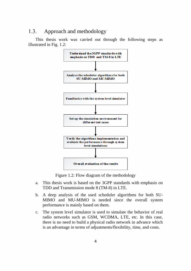
This thesis work was carried out through the following steps as

illustrated in Fig. 1.2:

Figure 1.2: Flow diagram of the methodology

a. This thesis work is based on the 3GPP standards with emphasis on

TDD and Transmission mode 8 (TM-8) in LTE.

b. A deep analysis of the used scheduler algorithms for both SU-

MIMO and MU-MIMO is needed since the overall system

performance is mainly based on them.

c. The system level simulator is used to simulate the behavior of real

radio networks such as GSM, WCDMA, LTE, etc. In this case,

there is no need to build a physical radio network in advance which

is an advantage in terms of adjustments/flexibility, time, and costs.

5

d. Building and preparing the simulation environment for different test

cases requires some input parameters from the e-Node B and UEs

as well as the channel.

e. Verify and evaluate the performance by simulating the algorithms

for different scenarios as mentioned in Section 1.2.

f. Analyze the simulation results as a function of the number of UEs

that are scheduled, and provide some recommendations based on

the performance.

Previous related work

LTE has been developed by the Third-Generation Partnership Project

(3GPP) and was adopted to be the promising broadband technology for 4G

and future 5G mobile standards to replace both GSM (2G) and

WCDMA/HSPA (3G) standards. Initially, the International

Telecommunication Union (ITU) specifies LTE data rates to be up to

100Mbps and 1Gbps in high and low mobility applications, respectively, for

fourth generation (4G) mobile communication systems [1].

To meet those requirements, SU-MIMO and MU-MIMO schemes are

used in LTE technology. The only difference between those two is that in

the latter case, the e-Node B in LTE (the BS) sends independent data

streams to multiple users simultaneously in the same time-frequency

resources, while in the former case, each user is allocated by the BS its own

time-frequency resources. MU-MIMO can be achieved by spatially

separating multiple users.

Different multi-antenna technologies for LTE-Advanced are briefly

discussed in [2], including design targets, deployment scenarios, multi-

antenna setups, downlink and uplink design, and performance assessment

based on cell spectral efficiency and cell-edge user spectral efficiency. It

was shown in [2] that the cross-polarized antenna setup at the base station

outperforms the co-polarized one in terms of cell spectral efficiency while

the opposite is true for cell edge user spectral efficiency case. More

techniques related to MU-MIMO in LTE-Advanced are also introduced in

[3], [4], including design challenges, precoding, control signaling and

dynamic SU/MU-MIMO switching.

MU-MIMO combined with a frequency domain packet scheduler for

LTE downlink was studied in [5] and it was shown that MU-MIMO with

precoding always outperforms MU-MIMO without precoding in terms of

ergodic capacity. Other benefits offered by different precoding techniques

6

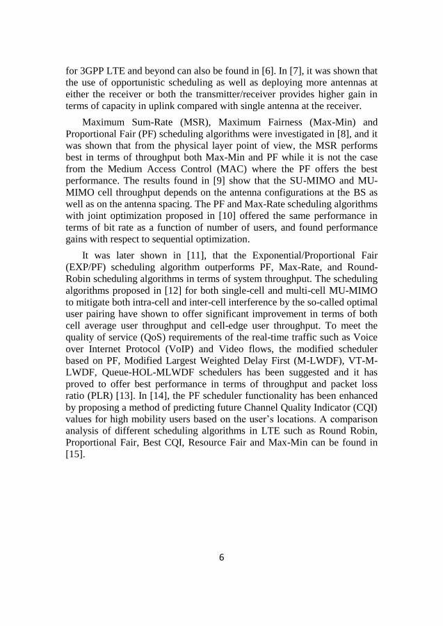
for 3GPP LTE and beyond can also be found in [6]. In [7], it was shown that

the use of opportunistic scheduling as well as deploying more antennas at

either the receiver or both the transmitter/receiver provides higher gain in

terms of capacity in uplink compared with single antenna at the receiver.

Maximum Sum-Rate (MSR), Maximum Fairness (Max-Min) and

Proportional Fair (PF) scheduling algorithms were investigated in [8], and it

was shown that from the physical layer point of view, the MSR performs

best in terms of throughput both Max-Min and PF while it is not the case

from the Medium Access Control (MAC) where the PF offers the best

performance. The results found in [9] show that the SU-MIMO and MU-

MIMO cell throughput depends on the antenna configurations at the BS as

well as on the antenna spacing. The PF and Max-Rate scheduling algorithms

with joint optimization proposed in [10] offered the same performance in

terms of bit rate as a function of number of users, and found performance

gains with respect to sequential optimization.

It was later shown in [11], that the Exponential/Proportional Fair

(EXP/PF) scheduling algorithm outperforms PF, Max-Rate, and Round-

Robin scheduling algorithms in terms of system throughput. The scheduling

algorithms proposed in [12] for both single-cell and multi-cell MU-MIMO

to mitigate both intra-cell and inter-cell interference by the so-called optimal

user pairing have shown to offer significant improvement in terms of both

cell average user throughput and cell-edge user throughput. To meet the

quality of service (QoS) requirements of the real-time traffic such as Voice

over Internet Protocol (VoIP) and Video flows, the modified scheduler

based on PF, Modified Largest Weighted Delay First (M-LWDF), VT-M-

LWDF, Queue-HOL-MLWDF schedulers has been suggested and it has

proved to offer best performance in terms of throughput and packet loss

ratio (PLR) [13]. In [14], the PF scheduler functionality has been enhanced

by proposing a method of predicting future Channel Quality Indicator (CQI)

values for high mobility users based on the user’s locations. A comparison

analysis of different scheduling algorithms in LTE such as Round Robin,

Proportional Fair, Best CQI, Resource Fair and Max-Min can be found in

[15].

7

Limitations

This thesis work has the following limitations:

SRS bandwidth: Sub-band SRS (24 x 4 PRBs). Due to limitations in

the simulator, we cannot consider sub-bands SRS.

MU-MIMO results for 1SRSAS UE and 1SRSWOAS UE Antenna

configurations and different periodicities are not included due to

time limitation.

Thesis outline

This thesis work is organized into 6 chapters. Chapter 1 is an

introduction. Chapter 2 reviews the general theoretical background

including 3GPP standards, MU-MIMO and scheduling in LTE. Chapter 3

briefly discusses the simulation framework for the scheduler algorithms

(SU-MIMO/MU-MIMO). Chapter 4 highlights the obtained results followed

by a discussion. Chapter 5 summarizes the main conclusions based on the

obtained results. Finally, Chapter 6 includes the future work related to the

project work.

8

9

2. Background Theory

MIMO antenna system configurations have shown to offer benefits in terms

of diversity gain, array gain (beamforming), and spatial multiplexing gain as

shown in Fig. 2.1 [16].

Diversity GainArray Gain

Spatial

Multiplexing

Gain

Figure 2.1: Benefits of MIMO [16]

Diversity overcomes fading by using multiple antennas at the receiver

(receive diversity) or at the transmitter (transmit diversity) to combine

coherently different fading signal paths.

Beamforming increases the received SINR by using multiple antenna

elements (antenna arrays) at the transmitter to focus the transmitted energy

towards the receiver. Receiver side beamforming is also possible.

Spatial Multiplexing increases the data rate by using multiple antennas

at both the transmitter and the receiver such that multiple data streams are

transmitted over parallel channels.

To reap the benefits of MIMO, recent 3GPP standards define novel

transceiver architectures that support multi-antenna techniques. We describe

these architectures below.

10

The 3GPP standards

Fig. 2.2 shows the generic block diagram for the downlink physical

channel processing [17].

Figure 2.2: Downlink physical channel processing [17]

Scrambling: Coded bits in each of the codewords to be transmitted

on a physical channel are scrambled.

Modulation/Layer mapping: Scrambled bits are modulated (QPSK,

16QAM, 64QAM, 256QAM) to produce complex symbols and

these are mapped onto one or several transmission layers.

Precoding: Complex symbols are for transmission on the antenna

ports.

Resource element mapping: Precoded complex symbols at each

antenna port are mapped to resource elements.

OFDM signal generation: OFDM symbols for each antenna port are

generated.

Codewords in Fig. 2.2 are generated through the following steps [18]:

Transport block CRC attachment

Code block segmentation and code block CRC attachment

Channel coding (Turbo coding)

Rate matching

Code block concatenation

Fig. 2.3 shows the general structure for uplink physical channel

processing [17].

11

Figure 2.3: Uplink physical channel processing [17]

Scrambling: Coded bits in each of the codewords to be transmitted

on a physical channel are scrambled.

Modulation/Layer mapping: Scrambled bits are modulated (QPSK,

16QAM, 64QAM) to produce complex symbols and these are

mapped onto one or several transmission layers.

Transform precoding (TP)/Precoding: Complex symbols are

precoded on each layer for transmission on the antenna ports after

transform precoding.

Resource element (RE) mapping/SC-FDMA generation: Precoded

complex symbols are mapped to resource elements and SC-FDMA

symbols for each antenna port are generated.

Codewords in Fig. 2.3 are generated according to [18] through the

following steps:

Transport block CRC attachment

Code block segmentation and code block CRC attachment

Channel coding of UL-SCH

Rate matching

Code block concatenation and channel coding (Turbo coding)

Data and control multiplexing

Channel interleaver.

2.1.1. Frame structure

3GPP defines three radio frame structures of 10 ms duration (each radio

frame) as follows [16], [17]:

Type 1 used in Frequency Division Duplex (FDD) mode only.

Type 2 used in Time Division Duplex (TDD) mode only.

12

Type 3 used in Licensed Assisted Access (LAA) secondary cell

operation only.

In this thesis work, only frame structure type 2 is considered. In TDD

mode, both uplink and downlink transmissions occur in the same frequency

band but at different time periods. Frame structure type 2 is illustrated in

Fig. 2.4.

Figure 2.4: Frame structure type 2 (switch-point periodicity = 5ms) [17]

Each radio frame duration (Tf) is 10 ms long and consists of 2 half-

frames of length equal to 5 ms (each half-frame). Each half-frame consists

of 5 subframes of length equal to 1 ms each. Thus, one radio frame is made

up of 10 consecutive subframes numbered from 0 to 9.

Frame structure type 2 defines a special subframe for downlink-to-

uplink switch, which comes in two periodicities: 5 ms and 10 ms. With 5 ms

downlink-to-uplink switch-point periodicity, the special subframe occurs in

both half-frames; with 10 ms downlink-to-uplink switch-point periodicity,

the special subframe occurs in the first half-frame only. Subframes zero,

five and the downlink part of special subframe (DwPTS) are always

associated with downlink transmissions, while the Uplink part of special

subframe (UpPTS) and the subframe immediately succeeding the special

subframe are always associated with uplink transmissions. GP denotes the

guard period between DwPTS and UpPTS.

From the above rules, many uplink-downlink configurations for radio

frame type 2 are possible. These are listed in Appendix 2.A, where "D"

denotes a subframe associated with downlink transmissions, "U" a subframe

associated with uplink transmissions, and "S" a special subframe containing

the three parts: DwPTS, GP and UpPTS discussed above [17]. In this thesis

work, we are solely concerned with uplink-downlink configuration 2 (see

Appendix 2.A).

2.1.2. Physical resource block

A physical resource block (PRB) is the smallest unit of resources that

can be allocated to one UE, and extends in both time and frequency

domains.

13

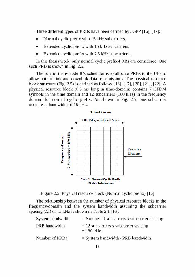
Three different types of PRBs have been defined by 3GPP [16], [17]:

Normal cyclic prefix with 15 kHz subcarriers.

Extended cyclic prefix with 15 kHz subcarriers.

Extended cyclic prefix with 7.5 kHz subcarriers.

In this thesis work, only normal cyclic prefix-PRBs are considered. One

such PRB is shown in Fig. 2.5.

The role of the e-Node B’s scheduler is to allocate PRBs to the UEs to

allow both uplink and downlink data transmissions. The physical resource

block structure (Fig. 2.5) is defined as follows [16], [17], [20], [21], [22]: A

physical resource block (0.5 ms long in time-domain) contains 7 OFDM

symbols in the time domain and 12 subcarriers (180 kHz) in the frequency

domain for normal cyclic prefix. As shown in Fig. 2.5, one subcarrier

occupies a bandwidth of 15 kHz.

Figure 2.5: Physical resource block (Normal cyclic prefix) [16]

The relationship between the number of physical resource blocks in the

frequency-domain and the system bandwidth assuming the subcarrier

spacing (Δf) of 15 kHz is shown in Table 2.1 [16].

System bandwidth = Number of subcarriers x subcarrier spacing

PRB bandwidth = 12 subcarriers x subcarrier spacing

= 180 kHz

Number of PRBs = System bandwidth / PRB bandwidth

14

This means that there are 6, 15, 25, 50, 75 and 100 PRBs for 1.4, 3, 5,

10, 15 and 20 MHz system bandwidths respectively.

Table 2.1: Physical resource blocks vs system bandwidth [16]

System bandwidth (MHz) 1.4 3 5 10 15 20

PRBs (Frequency-domain) 6 15 25 50 75 100

2.1.3. Concept of antenna ports in LTE (Downlink)

3GPP introduced the concept of antenna ports in downlink (e-Node B to

UE) where one resource grid per antenna port is used and the antenna ports

are determined by the reference signal configuration in the cell [17].

Table 2.2 summarizes the different antenna ports configuration with

their corresponding supported reference signals [17]:

Cell-specific reference signals (CRS) are sent on antenna port(s) 0,

{0,1} and {0,1,2,3}.

Downlink demodulation reference signals (DM-RS(DL)), sometimes

referred to as UE-specific reference signals associated with physical

downlink shared channel (PDSCH), are sent on antenna port(s) 5, 7,

8, 11, 13, {11,13} or {7,8,9,10,11,12,13,14}.

Table 2.2: Antenna ports and their respective downlink reference signals

[17]

Antenna port(s) 0 {0-1} {0-3} 5,7,8,11,13 {11,13} {7-14}

Reference signals CRS UE-specific reference signals

(DM-RS(DL))

In this thesis work, antenna ports {0,1} are considered for CRS while

for UE-specific reference signals, antenna ports {7,8}. Next we show the

resources grids associated with these antenna ports.

Fig. 2.6 illustrates the resource grid of CRS reference signals

transmitted on antenna ports 𝑝 ∈ {0,1} where 𝑅𝑝 denotes a resource element

corresponding to antenna port 𝑝.

15

Figure 2.6: Two-antenna port configuration for CRS (Normal cyclic prefix)

[17]

Fig. 2.7 illustrates the resource grid of UE-specific reference signals

(DM-RS(DL)), transmitted on antenna ports 𝑝 ∈ {7,8} where 𝑅𝑝 denotes a

resource element corresponding to antenna port 𝑝.

Figure 2.7: Antenna port configuration for UE-specific reference signals,

antenna ports 7 and 8 (Normal cyclic prefix) [17]

2.1.4. Concept of antenna ports in LTE (Uplink)

Like the downlink case (see Section 2.1.3), 3GPP introduced also the

concept of antenna ports in uplink (UE to e-Node B) where one resource

grid per antenna port is used. The antenna ports that are used for

16

transmission of physical channel or signal are determined by the number of

antenna ports as shown in Table 2.3 where [17]:

The physical uplink shared channel (PUSCH) and SRS use the same

antenna ports 10, {20,21} and {40,41,42,43}.

The physical uplink control channel (PUCCH) and uplink

demodulation reference signals (DM-RS(UL)) use antenna ports 100

and {200,201}.

Table 2.3: Antenna ports for different physical channels and signals [17]

Antenna port(s) 10 {20,21} {40-43} 100 {200-201}

Physical channel

or signal PUSCH/SRS PUCCH/DM-RS(UL)

In this thesis work, antenna ports 10 and {20-21} are considered for

PUSCH/SRS while for PUCCH/DM-RS(UL), antenna ports 100, {200-201}.

Fig. 2.8 illustrates the DM-RS(UL) structure (Normal cyclic prefix), sent

in each uplink slot (fourth symbol).

Figure 2.8: DM-RS(UL) structure (Normal cyclic prefix) [16], [20], [21], [22]

With frame structure type 2 (TDD), SRS sequences are sent in uplink

subframes, or in special subframes (uplink part). SRS configurations are

17

defined for full bandwidth (Non-frequency hopping SRS), or for sub-bands

(Frequency hopping SRS), as shown in Fig. 2.9 - 2.10 [16], [20], [21], [22].

Figure 2.9: Full bandwidth (96 PRBs) SRS configuration and 5 ms SRS

(sounding) periodicity

Figure 2.10: Sub-bands (24 PRBs) SRS configuration and 5 ms SRS

(sounding) periodicity

2.1.5. Transmission modes in LTE

Different downlink transmission modes (1 to 10) are specified by 3GPP

for LTE [19]. In this thesis work, only transmission mode 8 (TM-8), based

on dual layer transmission using ports 7 and 8, is considered; see Table 2.4.

18

TM-8 supports beamforming. In TDD operation, the e-Node B

computes the beamforming weights from the SRS by exploiting channel

reciprocity [16].

Table 2.4: Transmission mode 8 [19]

Transmission

mode

Transmission scheme

of PDSCH

TM-8

Single-antenna port, port 0 or Transmit diversity

(DCI Format 1A)

Dual layer transmission, ports 7 and 8 or Single-

antenna port, port 7 or 8 (DCI Format 2B)

TM-8 in LTE downlink is described in detail in Appendix 2.B. For the

uplink case, the different transmission modes (mode 1 and mode 2)

specified by 3GPP are given in Table 2.5 [19].

Table 2.5: Basic PUSCH transmission modes [19]

Transmission mode Transmission scheme of PUSCH

Mode 1 Single-antenna port, port 10

Mode 2

Single-antenna port, port 10

Closed-loop spatial multiplexing

2.1.6. Beamforming

As mentioned at the beginning of Sec. 2, transmitter-side beamforming

increases the received SINR by using multiple antenna elements at the

transmitter to focus the transmitted energy towards the receiver.

In Fig. 2.11, an e-Node B uses an antenna array to “beamform”

transmissions to specific UEs [16].

A description of antenna array configurations used in the simulations

can be found in Sec 3.4.

19

Figure 2.11: Illustration of beamforming (BS side) [16]

Multi-user Multiple Input Multiple Output (MU-

MIMO)

The main difference between SU-MIMO and MU-MIMO is illustrated

in Fig. 2.13-2.14. In SU-MIMO, time-frequency resource is allocated to a

single user communicating with the e-Node B. In MU-MIMO, different UEs

can communicate with the e-Node B using the same time-frequency

resource by the so-called spatial separation [1].

Figure 2.12: Illustartion of SU-MIMO (left), and MU-MIMO (right) [1]

With MU-MIMO, several users can communicate with the BS in the

same time-frequency resource.

20

2.2.1. System model

A general downlink MU-MIMO system is shown in Fig. 2.15 having a

BS (e-Node B) equipped with MT antennas and K UEs each equipped with

MR antennas (usually 1 or 2) in a cell. For the sake of argument, we let MR =

1 below.

Figure 2.13: System model

We assume a frequency flat channel given by the 𝐾 × 𝑀𝑇 channel

matrix 𝐻 = [ℎ1𝑇 …ℎ𝐾

𝑇 ]𝑇, where ℎ𝑘 is the 1 × 𝑀𝑇 MISO channel of user 𝑘.

The input-output relation of the MU-MIMO channel is given by [26]:

𝑦 = √𝐸𝑠𝐻𝑠 + 𝑛, (2.1)

Where 𝑠 is the 𝑀𝑇 × 1 vector of precoded transmitted symbols

satisfying 𝐸{𝑠𝐻𝑠} = 1, 𝑦 the 𝐾 × 1 vector of symbols received by the UEs,

𝑛 a 𝐾 × 1 UE noise vector with zero-mean circularly symmetric complex

Gaussian (ZMCSCG) independent entries with variance 𝑁0, and 𝐸𝑠 is the

total average energy available at the BS in one symbol period.

Linear precoding is sometimes assumed, both for its effectiveness and

analytical simplicity. With linear precoding at the BS, 𝑠 takes on the form:

𝑠 = 𝑊𝑥, (2.2)

Where 𝑊 is a 𝑀𝑇 × 𝐾 precoding matrix, and 𝑥 = [𝑥1, … , 𝑥𝐾]𝑇 with 𝑥𝑘

the data symbol of user 𝑘, which we assume ZMCSCG distributed with unit

variance. Inserting (2.2) into (2.1), we obtain:

21

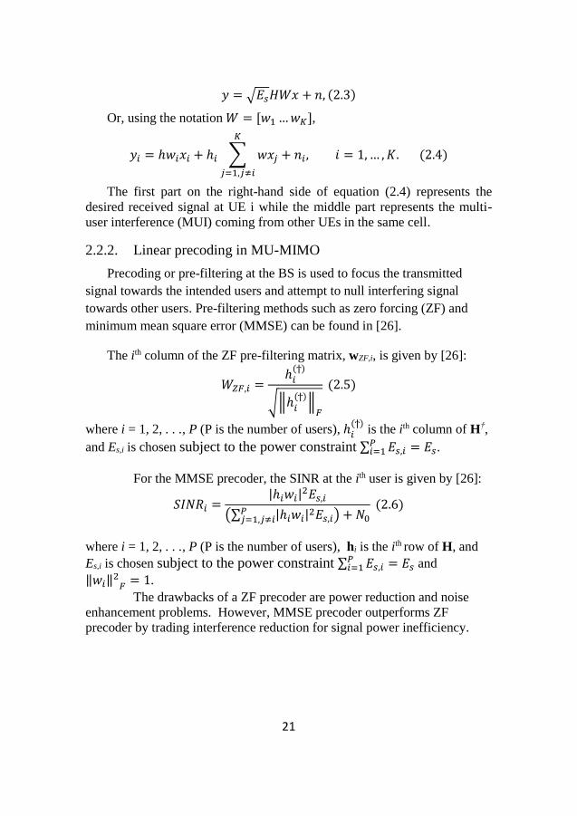
𝑦 = √𝐸𝑠𝐻𝑊𝑥 + 𝑛, (2.3)

Or, using the notation 𝑊 = [𝑤1 …𝑤𝐾],

𝑦𝑖 = ℎ𝑤𝑖𝑥𝑖 + ℎ𝑖 ∑ 𝑤𝑥𝑗

𝐾

𝑗=1,𝑗≠𝑖

+ 𝑛𝑖, 𝑖 = 1,… , 𝐾. (2.4)

The first part on the right-hand side of equation (2.4) represents the

desired received signal at UE i while the middle part represents the multi-

user interference (MUI) coming from other UEs in the same cell.

2.2.2. Linear precoding in MU-MIMO

Precoding or pre-filtering at the BS is used to focus the transmitted

signal towards the intended users and attempt to null interfering signal

towards other users. Pre-filtering methods such as zero forcing (ZF) and

minimum mean square error (MMSE) can be found in [26].

The ith column of the ZF pre-filtering matrix, wZF,i, is given by [26]:

𝑊𝑍𝐹,𝑖 =ℎ𝑖

(ϯ)

√‖ℎ𝑖(ϯ)

‖𝐹

(2.5)

where i = 1, 2, . . ., P (P is the number of users), ℎ𝑖(ϯ)

is the ith column of H†,

and Es,i is chosen subject to the power constraint ∑ 𝐸𝑠,𝑖𝑃𝑖=1 = 𝐸𝑠.

For the MMSE precoder, the SINR at the ith user is given by [26]:

𝑆𝐼𝑁𝑅𝑖 =|ℎ𝑖𝑤𝑖|

2𝐸𝑠,𝑖

(∑ |ℎ𝑖𝑤𝑖|2𝐸𝑠,𝑖

𝑃𝑗=1,𝑗≠𝑖 ) + 𝑁0

(2.6)

where i = 1, 2, . . ., P (P is the number of users), hi is the ith row of H, and

Es,i is chosen subject to the power constraint ∑ 𝐸𝑠,𝑖𝑃𝑖=1 = 𝐸𝑠 and

‖𝑤𝑖‖2𝐹

= 1.

The drawbacks of a ZF precoder are power reduction and noise

enhancement problems. However, MMSE precoder outperforms ZF

precoder by trading interference reduction for signal power inefficiency.

22

Scheduling in LTE

The main task of the scheduler is to determine how the shared time-

frequency resources should be allocated to different UEs. To accomplish

this task, both uplink and downlink schedulers are implemented in the e-

Node B. The scheduling decisions are often taken every Transmission Time

Interval (TTI), i.e. one millisecond [20], [21], [22].

The downlink scheduler determines which UEs upon which the DL-

SCH should be transmitted by assigning time-frequency resources

to them.

The uplink scheduler determines which UEs should transmit on

their UL-SCH by assigning time-frequency resources to them.

2.3.1. Scheduling strategies

Different scheduling strategies such as Max-C/I (or maximum rate),

Round Robin (RR) and Proportional Fair (PF) have been briefly discussed

in [20], [21], [22]. In this thesis work, only the RR scheduler is considered.

Its principle is based on assigning time-frequency resources to different UEs

in a cyclic fashion for the same amount of time without considering the

channel conditions experienced by different UEs [20], [21], [22].

2.3.2. Downlink packet scheduling in LTE

As mentioned earlier, the uplink and downlink schedulers are in the e-

Node B. Scheduling decisions are taken every TTI (1 ms) by allocating

time-frequency resources to different UEs. These resources are in the data

region while the downlink and uplink scheduling information is in the

control region of the downlink subframe. Within 1 ms, the control region

occupies 1 to 4 OFDM symbols (usually 3) which is indicated by the

Physical Control Format Indicator Channel (PCFICH) and the data region

where the Physical Downlink Shared Channel (PDSCH) is located, occupies

the remaining OFDM symbols (usually 11), as shown in Fig. 2.14 [27].

Control Region: 3 OFDM signals dedicated to signaling information

Data Region: Remaining 11 OFDM signals used for data transmission

23

Figure 2.14: Time-Frequency structure of the LTE downlink subframe

(example with 3 OFDM symbols dedicated to control channels) [27]

The control region contains the following downlink physical channels:

Physical Control Format Indicator Channel (PCFICH), Physical Hybrid-

ARQ Indicator Channel (PHICH) and Physical Downlink Control Channel

(PDCCH), while in the data region, there are: Physical Downlink Shared

Channel (PDSCH) and Physical Broadcast Channel (PBCH) [28].

From scheduling point of view, the PDCCH and PDSCH are the ones of

main interest. The PDCCH carries the downlink control information (DCI)

indicating where the downlink (DL) and uplink (UL) scheduling

information is located. This DCI message informs UE devices where to find

their data on the PDSCH [27], [28]. Different DCI formats used for

scheduling and power control purposes are listed in Table 2.6. In this thesis

work, DCI format 2B is the one which will be considered. It is associated

with transmission mode 8 (TM-8) and used for scheduling with dual layer

transmission as shown in Table 2.6.

24

Table 2.6: Supported DCI formats in REL. 8–11 [28]

DCI Formats Purpose

UL

Scheduling

(PUSCH)

0 UL Scheduling + TPC (PUSCH)

4 UL Scheduling with CLSM + TPC

(PUSCH) (Rel. 10-11)

DL

Scheduling

(PDSCH)

1 Scheduling, TPC (PUCCH)

1A Compact Scheduling with TxD, TPC

(PUCCH)

1B Compact Scheduling with CLSM, TPC

(PUCCH)

1C Very Compact Scheduling

1D Compact Scheduling with MU-MIMO,

TPC (PUCCH)

2 Scheduling with CLSM or TxD, TPC

(PUCCH)

2A Scheduling with Large CDD or TxD,

TPC (PUCCH)

2B Scheduling with Dual Layer

Transmission, TPC (PUCCH) (Rel. 9-11)

2C Up to 8 Layered Compact Scheduling,

TPC (PUCCH) (Rel. 10-11)

2D Up to 8 Layered Compact Scheduling

for CoMP, TPC (PUCCH) (Re. 11)

UL Power

Control

3 TPC for PUCCH, PUSCH 2bit Power

Adjustment

3A TPC for PUCCH, PUSCH 1bit Power

Adjustment

In Table 2.6, we have used the following abbreviations:

TPC: Transmit Power Control

CLSM: Closed Loop Spatial Multiplexing

TxD: Transmit Diversity

MU-MIMO: Multi-User MIMO

CDD: Cyclic Delay Diversity

CoMP: Co-ordinated Multi Point

25

2.3.3. Downlink (DL) resource allocation

Three types of DL resource allocation supported by LTE are defined

[28]: Type 0, Type 1, and Type 2; but only Type 0 will be considered in this

thesis work. DL resource allocation Type 0’s bits and associated DCI

formats are given in Table 2.7. Type 0 is indicated by setting the “resource

allocation header” field to 0.

The number of resources to be allocated in downlink within a subframe

(or TTI = 1 ms) is given by [28]:

𝑅𝐴 =𝑁𝑅𝐵

𝐷𝐿

𝑃,

Where RA denotes the Resource Assignment, 𝑁𝑅𝐵𝐷𝐿 is the system

bandwidth (BW) in terms physical resource blocks (PRBs) available in

downlink, P is the resource block group (RBG) size.

Table 2.7: DL resource allocation Type 0 with DCI formats 2/2A/2B/2C/2D

[28]

Bits DCI format 2/2A/2B*/2C*/2D*

0 to 3 Carrier Indicator in Rel. 10-11

1 Resource allocation header: Set to 0

[𝑵𝑹𝑩

𝑫𝑳

𝑷]

Resource Allocation Type 0

[𝑁𝑅𝐵

𝐷𝐿

𝑃]: Resource Assignment

2 UL Power Control (PUCCH)

2 Downlink Assignment Index (TDD DL/UL Configuration

1-6)

3 or 4 HARQ process number: 3 bits (FDD), 4 bits (TDD)

1 or 3

1 bit: Codeword Swap Flag or Scrambling Identity

3 bits: Antenna port(s), Scrambling Identity, # layer in Rel.

10-11

0 or 1 SRS Request only for TDD mode in Rel. 10-11

8+8 For transport block 1 & 2: 5 bits (MCS) + 1 bit (New data

indicator) + 2 bits (Redundancy version)

0, 2,

3, 6

DCI Format 2 Closed Loop MIMO: 3 (# Ant. ports 2), 6

(# Ant. ports 4)

DCI Format 2A Open Loop MIMO: 0 (# Ant. ports 2), 2

(# Ant. ports 4)

2 DCI Format 2D*: PDSCH RE Mapping and Quasi-Co-

Location Indicator

2 HARQ-ACK resource offset only for EPDCCH in Re. 11

26

As shown in Fig. 2.15, P is uniquely determined by 𝑁𝑅𝐵𝐷𝐿. Up to 25

RBGs (numbered from RBG 0 to RBG 24) are allocated in downlink within

a system bandwidth of 100 MHz where each RBG is equal to 4 PRBs as

indicated by the parameter P. P = 4 in this case [28]. Within 100 MHz, there

are 100 PRBs with each PRB having 12 subcarriers (180 kHz) in 0.5 ms.

Figure 2.15: DL resource allocation type 0 [28]

Fig. 2.16 illustrates DL SU-MIMO scheduling and DL MU-MIMO

scheduling (Resource Allocation Type 0 for 3 UEs: UE1, UE2 & UE3) with

the following examples:

Full-Buffer (FB) traffic: In SU-MIMO, 25 RBGs are allocated to

each UE every TTI, while in MU-MIMO, 3 users are paired (co-

scheduled) and allocated same 25 RBGs. In FB traffic case, UEs

send or receive data all time.

File Transfer Protocol (FTP) traffic: In SU-MIMO, UE1 needs 4

RBGs, UE2 needs 3 RBGs and UE3 needs 2 RBGs in 1 TTI, while

in MU-MIMO, UE1 needs 4 RBGs, UE2 needs 7 RBGs and UE3

needs 9 RBGs because of MU-pairing in 1 TTI. In FTP traffic case,

UEs send or receive according to their buffer size status, e.g. 1 kB,

10 kB, 100 kB, 1 MB and so on.

27

Figure 2.16: DL SU-MIMO scheduling vs DL MU-MIMO scheduling

28

29

3. Simulation Framework

In this thesis work, the performance evaluation is based on system level

simulations. The simulation framework is organized according to Fig. 3.1.

Channel model &

EnvironmentScenarios setup

Scheduler Algorithms

(SU-MIMO/MU-MIMO)Test cases

Figure 3.1: Simulation framework

Channel model and environment: Spatial channel models (SCM)

and urban macro environment are considered (see Section 3.1).

Scenario setup: Scenarios setup includes the system cell deployment

and system configurations parameters (see Section 3.2).

Scheduler algorithms for SU/MU-MIMO: Scheduler algorithms for

SU/MU-MIMO are based on precoding considering ICI, and

without considering ICI (see Section 3.3).

Test cases: Test cases are based on different parameters (see Section

3.4).

Channel model and environment

In this section, the spatial channel model (SCM) and the urban macro

(UMa) environment are succinctly described.

3.1.1. Channel model

For simulation purposes in this thesis work, we use the 3GPP SCM

channel model described in [23], [24], [25]. Two types of SCM are

considered:

Two dimensional (2D) SCM [25]

Three dimensional (3D) SCM [23], [24]

The main 2D SCM parameters at both the base station (BS) side and

mobile station (MS) side are given in Table 3.1.

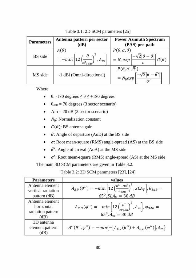
30

Table 3.1: 2D SCM parameters [25]

Parameters Antenna pattern per sector

(dB)

Power Azimuth Spectrum

(PAS) per-path

BS side

𝐴(𝜃)

= −𝑚𝑖𝑛 [12 (𝜃

𝜃3𝑑𝐵)2

, 𝐴𝑚]

𝑃(𝜃, 𝜎, �̅�)

= 𝑁0𝑒𝑥𝑝 [−√2|𝜃 − �̅�|

𝜎]𝐺(𝜃)

MS side -1 dBi (Omni-directional)

𝑃(𝜃, 𝜎′, 𝜃 ′̅)

= 𝑁0𝑒𝑥𝑝 [−√2|𝜃 − 𝜃 ′̅|

𝜎′]

Where:

θ: -180 degrees ≤ θ ≤ +180 degrees

θ3dB = 70 degrees (3 sector scenario)

Am = 20 dB (3 sector scenario)

𝑁0: Normalization constant

𝐺(𝜃): BS antenna gain

�̅�: Angle of departure (AoD) at the BS side

𝜎: Root mean-square (RMS) angle-spread (AS) at the BS side

𝜃 ′̅: Angle of arrival (AoA) at the MS side

𝜎′: Root mean-square (RMS) angle-spread (AS) at the MS side

The main 3D SCM parameters are given in Table 3.2.

Table 3.2: 3D SCM parameters [23], [24]

Parameters values

Antenna element

vertical radiation

pattern (dB)

𝐴𝐸,𝑉(𝜃′′) = −𝑚𝑖𝑛 [12(𝜃′′−900

𝜃3𝑑𝐵)2

, 𝑆𝐿𝐴𝑉], 𝜃3𝑑𝐵 =

650, 𝑆𝐿𝐴𝑉 = 30 𝑑𝐵

Antenna element

horizontal

radiation pattern

(dB)

𝐴𝐸,𝐻(𝜑′′) = −𝑚𝑖𝑛 [12 (𝜑′′

𝜑3𝑑𝐵)2

, 𝐴𝑚], 𝜑3𝑑𝐵 =

650, 𝐴𝑚 = 30 𝑑𝐵

3D antenna

element pattern

(dB) 𝐴′′(𝜃′′, 𝜑′′) = −𝑚𝑖𝑛{−[𝐴𝐸,𝑉(𝜃′′) + 𝐴𝐸,𝐻(𝜑′′)], 𝐴𝑚}

31

3.1.2. Environment

For our performance evaluation, we selected the “urban macro-cell”

environment of 3GPP SCM [25]. The path-loss (PL) for this environment is

given by:

𝑃𝐿 (𝑑𝐵) = 𝐴 + 𝐵 + 37.6 log10(𝑑) (3.1)

Where

A is the attenuation constant (15.3 dB)

B is the additional loss for indoor mobiles (20 dB)

d is the distance between BS and MS in meters

Table 3.3: Urban macro cell environment parameters [25]

Parameters Value

Number of paths (N) 6

Number of sub-paths (M) per-path 20

AS at BS (lognormal RV) 150 μAS = 1.18

εAS = 0.210

DS, lognormal RV) 0.65 μs

(RMS)

μDS = -6.18

εDS = 0.18

Angular spread scaling parameter (rAS) 1.3

Delay spread scaling parameter (rDS) 1.7

Lognormal shadowing standard deviation, σSF 8 dB

The main parameters defining the urban macro cell environment are

given in Table 3.3, where we have used the following abbreviations:

DS: Delay spread

AS: Angular spread

RMS: Root mean square

μAS: mean AS

εAS: AS standard deviation

μDS: mean DS

εDS: DS standard deviation

32

Scenario setup

3.2.1. System cell deployment

The system deployment is a 3GPP case 1 (Table 3.4) where the inter-

site distance (ISD) is equal to 500 meters [29].

Table 3.4: System cell deployment parameters

Parameters Value

Cell layout Hexagonal grid, 7 sites, 3 sectors per site

Inter-site distance (ISD) 500 meters

Carrier frequency 2 GHz

BS Max. Tx Power 40 watts or 46 dBm

Number of users (UEs) 210 (7 sites)/30 per site/10 per sector

3.2.2. System configurations parameters

The main system configuration parameters are given in Table 3.5.

Table 3.5: System configurations parameters

Parameters Value

System bandwidth 20 MHz (100 PRBs)

Frame structure Frame type 2 (TDD)

TDD configuration Uplink-Downlink configuration 2 (see Appendix 2.A)

Transmission

Mode TM-8 (2 layers-transmission & Beamforming)

Scheduler Round Robin (RR)

Scheduler algorithms for MU-MIMO

The following steps, illustrated in Fig. 3.2, briefly summarize the two

scheduler algorithms for MU-MIMO evaluated in this thesis work. These

are algorithm 1, which does not consider ICI, and algorithm 2, which does

consider ICI.

Note that, although the processing flow Fig. 3.2 addresses MU-MIMO

scheduling only, it can be easily adapted for SU-MIMO scheduling. This

can be accomplished by simply ignoring steps 3 and 4 (UEs spatial

separation, and MU-MIMO pairing blocks, respectively) whenever with

SU-MIMO scheduling is desired.

33

Figure 3.2: Scheduler algorithms for MU-MIMO

Step 1. UEs candidate list: The e-Node B creates a list of all candidate

UEs to be scheduled in a cell.

Step 2. Channel information and validation: The BS acquires the

channel information from UE’s SRS. For every UE candidate, the BS

validates that the channel information stored is not older than the report

periodicity value at the scheduling time.

Step 3. UEs spatial separation: This operation is based on the UEs

channel information, and UEs to be paired must have a sufficiently low

34

channel correlation (UEs separated in space) according to a certain

threshold value, the orthogonality factor (OF).

Step 4. MU-MIMO pairing: UEs with sufficiently low channel

correlation are the ones to be co-scheduled (paired).

Step 5. Precoding: The precoding operations, based on MMSE (see

Section 2.2.3), are done differently for the two algorithms, i.e., Algorithm 1

and Algorithm 2.

Step 6. SINR calculation: The SINR is calculated based on the

precoding.

Step 7. SINR to raw bit capacity: This operation maps between the

calculated SINR and lookup table to calculate the raw bit capacity.

Step 8. Resource allocation: Resources are allocated according to the

algorithms introduced to the reader in Section 2.3.3.

Step 9. Scheduling and link adaptation: The Scheduler will choose

the appropriate modulation and coding scheme (MCS) for this transmission.

Test cases

The simulated test cases are based on various parameters, including:

UEs traffic profile, SRS UL antenna configuration, BS ULA topology, SRS

bandwidth and sounding periodicity, and UEs’ moving speed. The values

taken by these parameters are given in Table 3.6.

Table 3.6: Test cases’ parameters

UEs traffic profile Full-Buffer/FTP

SRS UL antenna

configuration

2SRS UE

1SRSAS UE

1SRSWOAS UE

BS ULA topology 1x4x2 4x8x2

SRS bandwidth 96 PRBs

SRS periodicity 5 ms 10 ms 20 ms

UEs mobility 3 km/h 30 km/h 60 km/h

The SRS configurations considered, shown in Fig. 3.3, are: (a) Two

transmit SRS UE (2SRS UE), (b) one transmitting SRS UE with antenna

selection (1SRSAS UE), and (c) one transmitting SRS UE without antenna

selection (1SRSWOAS UE).

35

Tx1 Tx2

`

(a)

2 Tx. SRS

Tx

(b)

1 Tx. SRS WAS

Tx

(c)

1 Tx. SRS WOAS

Figure 3.3: (a) 2SRS UE, (b) 1SRSAS UE, (c) 1SRSWOAS UE

For 2SRS UE, two SRS are sent simultaneously to the BS from the two

UE’s antennas. For 1SRSAS UE, one SRS is sent to the BS from one UE

antenna at a given periodicity time, while another SRS is sent to the BS

from the other UE antenna at the next periodicity time, using an antenna

switch. Thus, for 1SRSAS UE, the actual SRS periodicity is doubled. For

1SRSWOAS UE, one SRS, which correspond to one of the dual layers, is

sent to the BS from one UE antenna at each periodicity time, while the other

layer information is estimated according to the orthogonality principle at the

BS.

The following base station uniform linear array (BSULA) topologies are

considered:

1x4x2 ULA topology (Fig. 3.4): This topology consists of one row

of four cross-polarized antenna elements (i.e. 8 antenna ports) with

a horizontal spacing dH = 0.5λ between antenna elements, where λ

is the wavelength at the carrier frequency.

4x8x2 ULA topology (Fig. 3.5): This topology consists of four rows

of eight cross-polarized antenna elements per row (i.e. 64 antenna

ports) with a horizontal spacing dH = 0.5λ and a vertical spacing dV

= 0.7λ between antenna elements, where λ is the wavelength at the

carrier frequency.

Figure 3.4: 1x4x2 ULA topology

36

Figure 3.5: 4x8x2 ULA topology

37

4. Results and Discussion

The simulation results are obtained through the following steps, illustrated

in Fig. 4.1 by means of a system level simulator:

Figure 4.1: Workflow using the system level simulator

Define simulator: This includes specifying the libraries to be

imported by the simulator. For example, radio network functions,

protocols, nodes, etc.

Set-up and run simulations: This includes setting parameter values

of the simulator radio network functions, defining traffic load, site

deployment, number of iterations (users), etc.

Log output and post-process logged output: This includes logging

the output from the simulation and post-processing of the logged

output e.g. by using MATLAB.

Analyze results: This means evaluating the outcomes form the

logged output for different test cases.

In this chapter, the logged output includes:

End to End (E2E) average downlink throughput per cell in

bits/second.

User throughput/BW vs. Average served traffic per cell/BW both in

bits/second/Hertz.

E2E downlink cell throughput description means serving cell downlink

throughput as measured by layer 3 (i.e., it does not include

MAC/RLC/HARQ).

All the curves are normalized by using the following same constants: ε

(average downlink throughput per cell), and α (UE throughput/BW vs.

Average cell throughput/BW).

As we have already mentioned, the algorithms for both SU-MIMO and

MU-MIMO are grouped into:

Algorithm 1: based on precoding without considering ICI

(WOCICI).

38

Algorithm 2: based on precoding considering ICI (WCICI)

The performance evaluation for both algorithms (SU/MU-MIMO) to be

considered is based on the following main test cases’ parameters:

UEs speed

SRS UL antenna configuration

SRS parameters (SRS bandwidth/SRS periodicity)

BS ULA topology

The purpose of this part is not only to evaluate the performance of the

system under consideration, but also to verify the correctness of some of the

functions in the system simulator, which is still under construction. Indeed,

several important bugs were found in various functions and reported to

Ericsson AB to be corrected.

The rest of this chapter is structured as follows. In Sec. 4.1, 4.2, and 4.3,

we present our results for SU-MIMO with FTP traffic profile and 8 BS

antenna elements, SU-MIMO with FB traffic profile and 64 BS antenna

elements, and MU-MIMO with FB traffic profile and 64 BS antenna

elements, respectively. Then, in Section 4.4 we present a comparative

analysis for these three cases.

SU-MIMO (FTP traffic profile and 8 BS antenna

elements)

The main simulation parameters for SU-MIMO with FTP traffic profile

and 8 BS antenna elements (BSULA topology: 1x4x2) are given in Table

4.1.

39

Table 4.1: Simulation parameters for SU-MIMO with FTP traffic profile

and 8 BS antenna elements (BSULA topology: 1x4x2)

System bandwidth 20MHz

Frame configuration TDD (2 UL subframes per frame)

Number of DL layers 2

Number of BS antenna

elements 8

Beamforming weights With and without considering ICI

Propagation model 2D SCM urban macro environment

7 sites x 3 sectors 21 cells, 3GPP case 1 (ISD 500m)

SRS (sounding)

bandwidth 96 PRBs (Full-bandwidth)

SRS (sounding)

periodicity (ms) [5, 10, 20]

SRS UL antenna

configuration 2SRS UE, 1SRSAS UE, 1SRSWOAS UE

UE speed (km/h) [3, 30, 60]

UE traffic profile

FTP (100 kilobytes), two downloads per UE

with mean time between them of 20 ms,

then the UE disconnects from the system

and a new UE enters after 100 ms.

Scheduling strategy Round Robin

Seeds 10, 10.005 seconds/seed

Number users as

iteration variable [1,7,14,21,42,63,84,105,210]

40


2SRS UE, 1SRSAS UE, 1SRSWOAS UE

Fig. 4.2 (2SRS UE), Fig. 4.3 (1SRSAS UE), and Fig. 4.4 (1SRWOAS

UE), illustrate average downlink throughput per cell, SU-MIMO case with

8 BS antenna elements, FTP traffic profile, 5 ms sounding periodicity, and

3, 30 and 60 km/h UE moving speeds.


elements @2SRS UE @5ms SRS periodicity @FTP


elements @1SRSAS UE @5ms SRS periodicity @FTP

41


elements @1SRSWOAS UE @5ms SRS periodicity @FTP

From Fig. 4.2, Fig 4.3, and Fig. 4.4, the following observations can be

made:

Fig. 4.2, Fig. 4.3, and Fig. 4.4: In general, the average downlink

throughput per cell decreases with increasing UE speeds for both

algorithms (WCICI & WOCICI) and that is because of larger

Doppler spreads.

Fig. 4.2: Algorithm 2 (WCICI) outperforms algorithm 1 (WOCICI)

in terms of average downlink throughput per cell for 3km/h UE

speed. However, for 30 and 60 km/h UE speeds, both algorithms

(WCICI & WOCICI) offer almost the same performance.

Fig. 4.3: Both algorithms (WCICI & WOCICI) offer almost the

same performance in terms of average downlink throughput per cell

for 3 km/h UE speed. However, for 30 and 60 km/h UE speeds,

algorithm 1 (WOCICI) outperforms slightly algorithm 2 (WCICI).


in terms of average downlink throughput per cell for 3km/h UEs

speed. However, for 30 and 60 km/h UE speeds, it is the opposite.

Fig. 4.5 (2SRS UE), Fig. 4.6 (1SRSAS UE), and Fig. 4.7 (1SRSWOAS

UE), illustrate User throughput vs. Average served traffic per cell, SU-

42

MIMO case with 8 BS antenna elements, FTP traffic profile, 5 ms sounding

periodicity, and 3, 30 and 60 km/h UE moving speeds.


MIMO_8 BS antenna elements @2SRS UE @5ms SRS periodicity @FTP



@FTP

43



@FTP

Fig. 4.5, Fig. 4.6, and Fig. 4.7 can be interpreted in the following way:

Fig. 4.5, Fig. 4.6, and Fig. 4.7: The number of UEs to be optimally

handled decreases with increasing UE speed for a given user

throughput-spectral efficiency threshold for both algorithms

(WCICI & WOCICI).

Fig. 4.5: For a user throughput-spectral efficiency threshold of 2α

bits/sec/Hz as an example, the system can handle optimally 84 UEs

with algorithm 1 (WOCICI) and 105 UEs with algorithm 2

(WCICI) for 3 km/h UE speed, and 63 UEs for 30 km/h UE speed

and 42 UEs for 60 km/h UE speed with both algorithms (WCICI &

WOCICI).



for 3 km/h UE speed and approximately 42 UEs for 30 and 60 km/h

UE speeds with both algorithms (WCICI & WOCICI).




UE speed with both algorithms (WCICI & WOCICI).

44


periodicity: 2SRS UE, 1SRSAS UE, 1SRSWOAS UE

Fig. 4.8 (2SRS UE), Fig. 4.9 (1SRSAS UE), and Fig. 4.10 (1SRWOAS

UE), illustrate average downlink throughput per cell, SU-MIMO case with

8 BS antenna elements, FTP traffic profile, 10 ms sounding periodicity, and

3, 30 and 60 km/h UE moving speeds.





45



From Fig. 4.8, Fig. 4.9, and Fig. 4.10, the following observations can be

made:

Fig. 4.8, Fig. 4.9, and Fig. 4.10: In general, the average downlink

throughput per cell decreases with increasing UE speeds for both


Doppler spreads.


in terms of average downlink throughput per cell for 3km/h UEs

speed. However, for 30 and 60 km/h UE speeds, both algorithms

(WCICI & WOCICI) offer almost the same performance.



for 3 km/h UE speed. However, for 30 and 60 km/h UE speeds,

algorithm 1 (WOCICI) outperforms slightly algorithm 2 (WCICI).

Fig. 4.10: Algorithm 2 (WCICI) outperforms algorithm 1

(WOCICI) in terms of average downlink throughput per cell for

3km/h UEs speed. However, for 30 and 60 km/h UE speeds, it is the

opposite.

46

Fig. 4.11 (2SRS UE), Fig. 4.12 (1SRSAS UE), and Fig. 4.13

(1SRSWOAS UE), illustrate User throughput vs. Average served traffic

per cell, SU-MIMO case with 8 BS antenna elements, FTP traffic

profile, 10 ms sounding periodicity, and 3, 30 and 60 km/h UE moving

speeds.





@FTP

47



@FTP

Fig. 4.11, Fig. 4.12, and Fig. 4.13 can be interpreted in the following

way:

Fig. 4.11, Fig. 4.12, and Fig. 4.13: The number of UEs to be

optimally handled decreases with increasing UE speed for a given

user throughput-spectral efficiency threshold for both algorithms

(WCICI & WOCICI).


bits/sec/Hz as an example, the system can handle optimally 84 for 3

km/h UEs speed and approximately 42 UEs for 30 km/h and 60

km/h UE speeds with both algorithms (WCICI & WOCICI).









48




(1SRWOAS UE), illustrate average downlink throughput per cell, SU-

MIMO case with 8 BS antenna elements, FTP traffic profile, 20 ms

sounding periodicity, and 3, 30 and 60 km/h UE moving speeds.





49



From Fig. 4.14, Fig. 4.15, and Fig. 4.16, the following observations can

be made:

Fig. 4.14, Fig. 4.15, and Fig. 4.16: In general, the average

downlink throughput decreases with increasing UE speeds for both


Doppler spreads.



3km/h UEs speed. However, for 30 and 60 km/h UE speeds, both

algorithms (WCICI & WOCICI) offer almost the same

performance.



for 3 km/h UE speed up to approximately 140 UEs. Above 140

UEs, algorithm 1 (WOCICI) outperforms algorithm 2 (WCICI).

However, for 30 and 60 km/h UE speeds, algorithm 1 (WOCICI)

outperforms slightly algorithm 2 (WCICI).



3km/h UEs speed. However, for 30 and 60 km/h UE speeds, it is the

opposite.

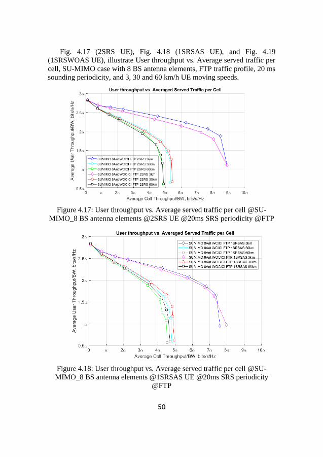
50


(1SRSWOAS UE), illustrate User throughput vs. Average served traffic per

cell, SU-MIMO case with 8 BS antenna elements, FTP traffic profile, 20 ms






@FTP

51



@FTP


way:




(WCICI & WOCICI).



for 3 km/h UEs speed and approximately 42 UEs for 30 km/h and

60 km/h UE speeds with both algorithms (WCICI & WOCICI).



for 3 km/h UE speed and approximately between 21 and 42 UEs for

30 and 60 km/h UE speeds with both algorithms (WCICI &

WOCICI).





52

SU-MIMO (Full-Buffer traffic profile and 64 BS

antenna elements)

The main simulation parameters for SU-MIMO with Full-Buffer traffic

profile and 64 BS antenna elements (BSULA topology: 4x8x2) are given in

Table 4.2.

Table 4.2: Simulation parameters for SU-MIMO with Full-Buffer traffic

profile and 64 BS antennas elements (BSULA topology: 4x8x2)



Number of DL

layers 2

Number of BS

antenna elements 64

Beamforming

weights With and without considering ICI

Propagation model 2D SCM Urban macro environment


SRS (sounding)


SRS (sounding)


SRS UL antenna

configuration

2SRS UE, 1SRSAS UE, 1SRSWOAS

UE

UE speed (km/h) [3, 30, 60]

UE traffic profile Full-Buffer



Number users as


53





MIMO case with 64 BS antenna elements, Full-Buffer traffic profile, 5 ms


Figure 4.20: Average downlink throughput/cell @SU-MIMO_64 BS

antenna elements @2SRS UE @5ms SRS periodicity @Full-Buffer


antenna elements @1SRSAS UE @5ms SRS periodicity @Full-Buffer

54


antenna elements @1SRSWOAS UE @5ms SRS periodicity @Full-Buffer

From Fig. 4.20, Fig. 2.21, and Fig. 2.22 the following observations can

be made:




Doppler spreads.


(WOCICI) in terms of average downlink throughput per cell for 3,

30 and 60 km/h UE speed.









per cell, SU-MIMO case with 64 BS antenna elements, Full-Buffer

traffic profile, 5 ms sounding periodicity, and 3, 30 and 60 km/h UE

moving speeds.

55



Buffer



@Full-Buffer

56



@Full-Buffer


way:




(WCICI & WOCICI).


bits/sec/Hz as an example, the system can handle approximately 63

UEs with algorithm 1 (WOCICI) and 84 UEs with algorithm 2

(WCICI) for 3 km/h UE speed, and 42 UEs with algorithm 1

(WOCICI) and 63 UEs with algorithm 2 (WCICI) for 30 km/h UE

speed, and approximately 42 UEs with both algorithms (WCICI &

WOCICI) for 60 km/h UE speed.



for 3 km/h UE speed, and 42 UEs for 30 and 60 km/h UE speeds

with both algorithms (WCICI & WOCICI).



with algorithm 1 (WOCICI) and 63 UEs with algorithm 2 (WCICI)

for 3 km/h UE speed, and 21 UEs with algorithm 1 (WOCICI) and

42 UEs with algorithm 2 (WCICI) for 30 km/h UE speed, and 21

57

UEs with both algorithms (WCICI & WOCICI) for 60 km/h UE

speed.








antenna elements @2SRS UE @10 ms SRS periodicity @Full-Buffer


antenna elements @1SRSAS UE @10 ms SRS periodicity @Full-Buffer

58


antenna elements @1SRSWOAS UE @10 ms SRS periodicity @Full-

Buffer


be made:




Doppler spreads.














moving speeds.

59


MIMO_64 BS antenna elements @2SRS UE @10ms SRS periodicity

@Full-Buffer



@Full-Buffer

60


MIMO_64 BS antenna elements @1SRSWOAS UE @10ms SRS

periodicity @Full-Buffer


way:


optimally handled decreases with increasing UE speed for a

given user throughput-spectral efficiency threshold for both

algorithms (WCICI & WOCICI).

Fig. 4.29: For a user throughput-spectral efficiency threshold of

10α bits/sec/Hz as an example, the system can handle

approximately 63 UEs with algorithm 1 (WOCICI) and 84 UEs

with algorithm 2 (WCICI) for 3 km/h UE speed, and 42 UEs

with algorithm 1 (WOCICI) and 63 UEs with algorithm 2

(WCICI) for 30 km/h, and 42 UEs with both algorithms

(WCICI & WOCICI) for 60 km/h UE speed.


10α bits/sec/Hz as an example, the system can handle optimally

63 UEs for 3 km/h UE speed, 42 UEs for 30 km/h UE speed,

and 21 UEs for 60 km/h UE speed with both algorithms

(WCICI & WOCICI).


10α bits/sec/Hz as an example, the system can handle optimally

61

42 UEs with algorithm 1 (WOCICI) and 63 UEs with algorithm

2 (WCICI) for 3 km/h UE speed, and 21 UEs with algorithm 1

(WOCICI) and 42 UEs with algorithm 2 (WCICI) for 30 km/h

UE speed, and 21 UEs with both algorithms (WCICI &








Figure 4.32: Average downlink throughput/Cell @SU-MIMO_64 BS

antenna elements @2SRS UE @20 ms SRS periodicity @Full-Buffer

62


antenna elements @1SRSAS UE @20 ms SRS periodicity @Full-Buffer


antenna elements @1SRSWOAS UE @20 ms SRS periodicity @Full-

Buffer


be made:

63




Doppler spreads.














moving speeds.


MIMO_64 BS antenna elements @2SRS UE @20ms SRS periodicity

@Full-Buffer

64



@Full-Buffer


MIMO_64 BS antenna elements @1SRSWOAS UE @20ms SRS

periodicity @Full-Buffer


way:

65




(WCICI & WOCICI).



with algorithm 1 (WOCICI) and 84 UEs with algorithm 2 (WCICI)

for 3 km/h UE speed, and 42 UEs with Algorithm 1 (WOCICI) and

approximately 63 UEs with algorithm 2 (WCICI) for 30 km/h UE

speed, and between 21 and 42 UEs with both algorithms (WCICI &



bits/sec/Hz as an example, the system can handle approximately 63

UEs with both algorithms (WCICI & WOCICI) for 3 km/h UE

speed, and 42 UEs for 30km/h UE speed, and 21 UEs for 60 km/h

UE speed with both algorithms (WCICI & WOCICI).



with Algorithm 1 (WOCICI) and 63 UEs with Algorithm 2

(WCICI) for 3 km/h UE speed, and between 21 and 42 UEs with

both algorithms (WCICI & WOCICI) for 30 and 60 km/h UE

speeds.

66

MU-MIMO (Full-Buffer traffic profile and 64 BS

antennas elements)

The main simulation parameters for MU-MIMO with Full-Buffer traffic

profile and 64 BS antennas elements (BSULA topology: 4x8x2) are given in

Table 4.3.

Table 4.3: Simulation parameters for MU-MIMO with Full-Buffer traffic

profile and 64 BS antennas elements (BSULA topology: 4x8x2)



Number of DL layers 2

Number of BS antenna

elements 64

Beamforming weights With and without considering ICI

Propagation model 2D SCM Urban macro environment


SRS (sounding)


SRS (sounding)


SRS UL antenna

configuration

2SRS UE, 1SRSAS UE,

1SRSWOAS UE

UE speed (km/h) [3, 30, 60]

UE traffic profile Full-Buffer



Number users as


Pairing limit 8 Layers (4 UEs with 2 layer each)

Orthogonality factor [0.1, 0.25, 1]

4.3.1. MU-MIMO @64 BS antenna elements @2 SRS UE, UE

speed: 3 km/h, Sounding periodicity: 5 ms

Fig. 4.38 (2SRS UE) illustrates average downlink throughput per cell,

MU-MIMO case with 64 BS antenna elements, Full-Buffer traffic profile, 5

ms sounding periodicity, and 3 km/h UE moving speeds.

67


@2SRS UE @5ms SRS periodicity @Full-Buffer

From Fig. 4.38, the following observations can be made:

Algorithm 2 (WCICI) outperforms algorithm 1 (WOCICI) in terms

of average downlink throughput per cell for orthogonality factor

(OF) value of 1 and 3 km/h UEs speed up to approximately 120

users. For orthogonality factor (OF) value of 0.25 and 3 km/h UEs

speed, algorithm 2 (WCICI) outperforms algorithm 1 (WOCICI) in

terms of average downlink throughput per cell up to approximately

140 users. For orthogonality factor (OF) value of 0.1 and 3 km/h

UEs speed, algorithm 2 (WCICI) outperforms algorithm

1(WOCICI) in terms of average downlink throughput per cell up to

approximately 170 users.

In general, a higher value of orthogonality factor (OF) implies a

higher average downlink throughput per cell.

Fig. 4.39 (2SRS UE) illustrates User throughput vs. Average served

traffic per cell, MU-MIMO case with 64 BS antenna elements, Full-Buffer

traffic profile, 5 ms sounding periodicity, and 3 km/h UE moving speeds.

68


MIMO @3 km/h @2SRS UE @5ms SRS periodicity @Full-Buffer

Fig. 4.39 can be interpreted in the following way:

In MU-MIMO with 3 km/h UE speed, for a user throughput-

spectral efficiency threshold of 10α bits/sec/Hz as an example, the

system can handle optimally 105 UEs with both algorithms (WCICI

& WOCICI) for orthogonality factor value (OF) of 1.

The number of UEs to be optimally handled in the system (MU-

MIMO) decreases with increasing UE speed (compare Fig. 4.33 and

Fig. 4.35).

When the curves start bending, we can consider this point as an

optimal performance of the system with the corresponding number

of users.

4.3.2. MU-MIMO @64 BS antenna elements @2 SRS UE, UE

speed: 30 km/h, Sounding periodicity: 5 ms

Fig. 4.40 (2SRS UE) illustrates average downlink throughput per cell,

MU-MIMO case with 64 BS antenna elements, Full-Buffer traffic profile, 5

ms sounding periodicity, and 30 km/h UE moving speeds.

69


@2SRS UE @5ms SRS periodicity @Full-Buffer

From Fig. 4.40, the following observations can be made:

Algorithm 2 (WCICI) outperforms algorithm 1(WOCICI) in terms

of average downlink throughput per cell for orthogonality factor

(OF) values of 0.25 and 1 and 30 km/h UEs speed up to

approximately 90 users. For orthogonality factor (OF) value of 0.1

and 30 km/h UEs speed, algorithm 2 (WCICI) outperforms

algorithm 1 (WOCICI) in terms of average downlink throughput per

cell up to approximately 140 users.

In contrast the 3 km/h case, a higher value of orthogonality factor

(OF) does not always imply a higher average downlink throughput

per cell for both algorithms for 30 km/h UEs speed.

Fig. 4.41 (2 SRS UE) illustrates User throughput vs. Average served

traffic per cell, MU-MIMO case with 64 BS antenna elements, Full-Buffer

traffic profile, 5 ms sounding periodicity, and 30 km/h UE moving speeds.

70


MIMO @30 km/h @2SRS UE @5ms SRS periodicity @Full-Buffer

Fig. 4.41 can be interpreted in the following way:

In MU-MIMO with 30 km/h UE speed, for a user throughput-

spectral efficiency threshold of 10α bits/sec/Hz as an example, the

system can handle optimally 63 UEs with both algorithms (WCICI

& WOCICI) for orthogonality factor value (OF) of 1.

The number of UEs to be optimally handled in the system (MU-

MIMO) decreases with increasing UE speed (compare Fig. 4.33 and

Fig. 4.35).

When the curves start bending, we can consider this point as an

optimal performance of the system with the corresponding number

of users.

Comparative analysis

In this section, the overall performance of both algorithms is

summarized based on maximum cell throughput for the following cases:

SU-MIMO (8 BS antenna elements and FTP traffic profile) in Section 4.4.1,

SU-MIMO (64 BS antenna elements and Full-Buffer) in Section 4.4.2, and

SU-MIMO vs. MU-MIMO (64 BS antenna elements and Full-Buffer traffic

profile) in Section 4.4.3.

71

4.4.1. SU-MIMO (8 BS antenna elements and FTP traffic profile)

Table 4.4 summarizes Fig. 4.2, Fig. 4.3, and Fig. 4.4.

Table 4.4: Summary (Fig. 4.2, Fig. 4.3, and Fig. 4.4)

SU-MIMO @8 BS

antenna elements @5

ms SRS periodicity

@FTP

Max_Thpt

(bps)

@3km/h

@105users

Max_Thpt

(bps)

@30km/h

@105users

Max_Thpt

(bps)

@60km/h

@105users

2SRS UE

WOCICI ~16.5ε ~13.5ε ~10.5ε

WCICI ~18ε ~13.5ε ~10.5ε

1SRSAS UE

WOCICI ~16.5ε ~11ε ~10ε

WCICI ~17ε ~11ε ~10ε

1SRSWOAS

UE

WOCICI ~14ε ~11.5ε ~10.5ε

WCICI ~14.5ε ~12ε ~10ε



SU-MIMO @8 BS

antenna elements @10

ms SRS periodicity

@FTP

Max_Thpt

(bps)

@3km/h

@105users

Max_Thpt

(bps)

@30km/h

@105users

Max_Thpt

(bps)

@60km/h

@105users

2SRS UE

WOCICI ~16.5ε ~12ε ~10ε


1SRSAS UE

WOCICI ~16ε ~10ε ~9.5ε

WCICI ~16ε ~10ε ~9.5ε

1SRSWOAS

UE

WOCICI ~14ε ~11ε ~10.5ε

WCICI ~14.5ε ~11ε ~10ε

72



SU-MIMO @8 BS


ms SRS periodicity

@FTP

Max_Thpt

(bps)

@3km/h

@105users

Max_Thpt

(bps)

@30km/h

@42users

Max_Thpt

(bps)

@60km/h

@42users

2SRS UE

WOCICI ~16ε ~10.5ε ~10.5ε

WCICI ~17ε ~10.5ε ~9.5ε

1SRSAS UE

WOCICI ~15ε ~10ε ~9.5ε

WCICI ~15ε ~10ε ~9.5ε

1SRSWOAS

UE

WOCICI ~13.5ε ~11ε ~10.5ε

WCICI ~14ε ~10.5ε ~9.5ε

From Table 4.4, Table 4.5, and Table 4.6, the following observations

can be made:

2 SRS UE offers the best performance in terms of maximum cell

throughput with both algorithms (WCICI & WOCICI) for 5, 10 and

20 ms SRS periodicities and all UE speeds.

1 SRSAS UE offers the medium performance in terms of maximum

cell throughput with both algorithms (WCICI & WOCICI) for 5, 10

and 20 ms SRS periodicities and pedestrian users (3 km/h UE

speed), but it is not the case for medium (30 km/h) and high (60

km/h) UE speeds where 1 SRSWOAS performs better that 1

SRSAS.

For pedestrian users (3 km/h UE speed), the effect of SRS

periodicity is negligible. However, for medium (30 km/h) and high

mobility users (60 km/h), the effect of SRS periodicity is somewhat

noticeable.

There is degradation of maximum cell throughput with increasing

SRS periodicity and UE speed.

73

4.4.2. SU-MIMO (64 BS antenna elements and Full-Buffer traffic

profile)



SU-MIMO @64 BS

antenna elements @5

ms SRS periodicity

@Full-Buffer

Max_Thpt

(bps)

@3km/h

@63users

Max_Thpt

(bps)

@30km/h

@63users

Max_Thpt

(bps)

@60km/h

@63users

2SRS UE

WOCICI ~54ε ~45ε ~41ε


1SRSAS UE



1SRSWOAS

UE





SU-MIMO @64 BS


ms SRS periodicity

@Full-Buffer

Max_Thpt

(bps)

@3km/h

@63users

Max_Thpt

(bps)

@30km/h

@63users

Max_Thpt

(bps)

@60km/h

@63users

2SRS UE



1SRSAS UE



1SRSWOAS

UE



74



SU-MIMO @8 BS


ms SRS periodicity

@Full-Buffer

Max_Thpt

(bps)

@3km/h

@105users

Max_Thpt

(bps)

@30km/h

@105users

Max_Thpt

(bps)

@60km/h

@105users

2SRS UE



1SRSAS UE



1SRSWOAS

UE



From Table 4.7, Table 4.8 and Table 4.9, the following observations can

be made:

2 SRS UE offers the best performance in terms of maximum cell

throughput with both algorithms (WCICI & WOCICI) for 5, 10 and

20 ms SRS periodicities and all UE speeds.

1 SRSAS UE offers the medium performance in terms of maximum

cell throughput with both algorithms (WCICI & WOCICI) for 5 and

10 SRS periodicities and different UE speeds but for 20 ms SRS

periodicity and medium and high UE speeds bot 1 SRSAS and

1SRSWOAS performs almost similarly.

There is degradation of maximum cell throughput with increasing

SRS periodicity and UE speed.

75

4.4.3. SU-MIMO vs. MU-MIMO (64 BS antenna elements and

Full-Buffer traffic profile)



2SRS UE @

64 BS antenna elements

@5ms SRS periodicity

@Full-Buffer

Max_Thpt

(bps)

@3km/h

@42users

Max_Thpt

(bps)

@30km/h

@42users

SU-MIMO WOCICI ~52ε ~43ε

WCICI ~80ε ~63ε

MU-MIMO

@OF=0.1

WOCICI ~65ε ~48ε

WCICI ~95ε ~68ε

MU-MIMO

@OF=0.25

WOCICI ~82ε ~54ε

WCICI ~125ε ~76ε

MU-MIMO

@OF=1

WOCICI ~90ε ~56ε

WCICI ~135ε ~80ε

From Table 4.10, the following observations can be made:

In MU-MIMO with 64 BS antenna elements, both algorithms offer

higher performance in terms of maximum cell throughput compared

with the same algorithms in SU-MIMO with 64 BS antenna

elements.

In MU-MIMO, a higher value of orthogonality factor implies higher

cell throughput for both algorithms.

In general, there is degradation of maximum cell throughput with

increasing UE speed.

76

77

5. Conclusions

The two discussed (in Chapter 4) algorithms for both SU-MIMO and

MU-MIMO are:

Algorithm 1: based on precoding that does not consider ICI

(WOCICI).

Algorithm 2: based on precoding that does consider ICI (WCICI).

Based on the obtained results, the following conclusions can be drawn

for both algorithms:

SU-MIMO (FTP)

WCICI performs better than WOCICI for pedestrian users (3

Km/h), for different SRS periodicities (5, 10 and 20 ms) and SRS

UL antenna configurations. However, and under the specific traffic

profiles used in the simulations, for medium (30 km/h) and high (60

km/h) UE speeds, it is better to use WOCICI since it performs

similarly or better than WCICI.

The performance of 1 SRSWOAS outperforms 1 SRSAS for

medium and high UE speeds.


increasing SRS periodicity and UE speed.

SU-MIMO (Full-Buffer)

WCICI performs better than WOCICI for pedestrian users (3

Km/h), medium (30 km/h) and high moving speed (60 km/h), for

different SRS periodicities (5, 10 and 20 ms) and SRS UL antenna

configurations.

The performances of 1 SRSWOAS and 1 SRSAS for high UE speed

are almost the same.


increasing SRS periodicity and UE speed.

78

MU-MIMO (Full-Buffer)

In our simulations, it always best to have an orthogonality factor of

one which means that we pair as many users as possible (maximum

number of UEs can be paired. This is because users are dropped

somewhat sparsely in the simulation area. With higher user loads,

other values of the orthogonality factor might work better.

WCICI case performs better WOCICI for low and medium load in

the system.

Similar to the SU-MIMO case, the cell throughput is decreased

when the UE’s speed is increased from 3 to 30 Km/h.

79

6. Future work

As already mentioned, this thesis work has been focusing on the following

main aspects:

Downlink SU/MU-MIMO

Transmission mode: TM-8 (2 layers’ transmission)

2 layers at the UE’s side

Traffic profile: Full-Buffer

SRS bandwidth: 96x1 PRBs (Full-bandwidth SRS configuration)

Scheduler: Round Robin (RR)

More aspects regarding scheduler algorithms for MU-MIMO not yet

investigated include:

Uplink SU/MU-MIMO

8 layers’ transmission, i.e. TM-9/10

1 layer at the UE’ side.

Sub-bands SRS configuration i.e. 24x4 PRBs

Other scheduling strategies such as Proportional Fair (PF), Max C/I

and so on.

Research proposals available in Section 1.4 (Previous related work).

80

References

[1] G. Bauch and G. Dietl, "Multi-user MIMO for achieving IMT-

Advanced requirements," 2008 International Conference on

Telecommunications, St. Petersburg, 2008, pp. 1-7.

[2] F. Boccardi et al., "Multiple-antenna techniques in LTE-advanced,"

in IEEE Communications Magazine, vol. 50, no. 3, pp. 114-121,

March 2012.

[3] L. Liu, R. Chen, S. Geirhofer, K. Sayana, Z. Shi and Y. Zhou,

"Downlink MIMO in LTE-advanced: SU-MIMO vs. MU-MIMO,"

in IEEE Communications Magazine, vol. 50, no. 2, pp. 140-147,

February 2012.

[4] C. Lim, T. Yoo, B. Clerckx, B. Lee and B. Shim, "Recent trend of

multiuser MIMO in LTE-advanced," in IEEE Communications

Magazine, vol. 51, no. 3, pp. 127-135, March 2013.

[5] Z. Lin, B. Vucetic and J. Mao, "Ergodic Capacity of LTE Downlink

Multiuser MIMO Systems," 2008 IEEE International Conference

on Communications, Beijing, 2008, pp. 3345-3349.

[6] K. C. Beh, C. Han, M. Nicolaou, S. Armour and A. Doufexi,

"Power Efficient MIMO Techniques for 3GPP LTE and

Beyond," 2009 IEEE 70th Vehicular Technology Conference Fall,

Anchorage, AK, 2009, pp. 1-5.

[7] W. Ajib and D. Haccoun, "An overview of scheduling algorithms in

MIMO-based fourth-generation wireless systems," in IEEE

Network, vol. 19, no. 5, pp. 43-48, Sept.-Oct. 2005.

[8] Yueming Cai, Jiang Yu, Youyun Xu and Mulin Cai, "A comparison

of packet scheduling algorithms for OFDMA systems," 2008 2nd

International Conference on Signal Processing and Communication

Systems, Gold Coast, 2008, pp. 1-5.

[9] A. Farajidana, W. Chen, A. Damnjanovic, T. Yoo, D. Malladi and

C. Lott, "3GPP LTE Downlink System

Performance," GLOBECOM 2009 - 2009 IEEE Global

Telecommunications Conference, Honolulu, HI, 2009, pp. 1-6.

[10] R. Kwan, C. Leung and J. Zhang, "Proportional Fair Multiuser

Scheduling in LTE," in IEEE Signal Processing Letters, vol. 16, no.

6, pp. 461-464, June 2009.

[11] H. A. M. Ramli, R. Basukala, K. Sandrasegaran and R.

Patachaianand, "Performance of well-known packet scheduling

algorithms in the downlink 3GPP LTE system," 2009 IEEE 9th

Malaysia International Conference on Communications (MICC),

Kuala Lumpur, 2009, pp. 815-820.

81

[12] L. Liu, Young-Han Nam and J. Zhang, "Proportional fair

scheduling for multi-cell multi-user MIMO systems," 2010 44th

Annual Conference on Information Sciences and Systems (CISS),

Princeton, NJ, 2010, pp. 1-6.

[13] D. Samia and B. Ridha, "A New Scheduling Algorithm for Real-

Time Communication in LTE Networks," 2015 IEEE 29th

International Conference on Advanced Information Networking and

Applications Workshops, Gwangiu, 2015, pp. 267-271.

[14] Qurat-ul-Ain, S. R. ul Hassnain, M. Shah and S. A. Mahmud, "An

evaluation of scheduling algorithms in LTE based 4G networks,"

2015 International Conference on Emerging Technologies (ICET),

Peshawar, 2015, pp. 1-6.

[15] A. Marinčić and D. Šimunić, "Performance evaluation of different

scheduling algorithms in LTE systems," 2016 39th International

Convention on Information and Communication Technology,

Electronics and Microelectronics (MIPRO), Opatija, 2016, pp. 595-

600.

[16] C. Johnson, Long Term Evolution in Bullets, second ed., Create

Space Independent Publishing Platform, July 2012.

[17] 3GPP36.211, “Evolved Universal Terrestrial Radio Access (E-

UTRA); Physical channels and modulation” 3GPP, Sophia

Antipolis, Technical Specification 36.211 v13.2.0, August 2016.


UTRA); Multiplexing and channel coding” 3GPP, Sophia Antipolis,

Technical Specification 36.212 v13.0.0, January 2016.


UTRA); Physical layer procedures” 3GPP, Sophia Antipolis,

Technical Specification 36.213 v13.0.0, May 2016.

[20] E. Dahlman et al., 3G Evolution: HSPA and LTE for Mobile

Broadband, 2nd ed., Academic Press, 2008.

[21] E. Dahlman, S. Parkvall, and J. Sköld, 4G: LTE/LTE Advanced for

Mobile Broadband, 2nd ed., Academic Press, 2014.

[22] E. Dahlman, S. Parkvall, and J. Sköld, 4G, LTE-Advanced Pro and

The Road to 5G, Academic Press, 2016.

[23] 3GPP TR 36.873,” Technical Specification Group Radio Access

Network; Study on 3D channel model for LTE” 3GPP, Sophia

Antipolis, Technical Report 36.873 v12.3.0, December 2016.


Network; Study on elevation beamforming / Full-Dimension (FD)

Multiple Input Multiple Output (MIMO) for LTE” 3GPP, Sophia

Antipolis, Technical Report 36.897 v13.0.0, June 2015.

82


Network; Spatial channel model for Multiple Input Multiple Output

(MIMO) simulations (Release 9)”, 3GPP, Sophia Antipolis,

Technical Report 25.996 V9.0.0, December 2009.

[26] Paulraj, Arogyaswami, Rohit Nabar, and Dhabanjay Gore,

Introduction to Space-Time Wireless Communications, Cambridge,

UK: Cambridge University Press, 2003.

[27] F. Capozzi, G. Piro, L. A. Grieco, G. Boggia and P. Camarda,

"Downlink Packet Scheduling in LTE Cellular Networks: Key

Design Issues and a Survey," in IEEE Communications Surveys &

Tutorials, vol. 15, no. 2, pp. 678-700, Second Quarter 2013.

[28] G. Ku and J. M. Walsh, "Resource Allocation and Link Adaptation

in LTE and LTE Advanced: A Tutorial," in IEEE Communications

Surveys & Tutorials, vol. 17, no. 3, pp. 1605-1633, third-quarter

2015.


Network; Further Advancements for E-UTRA Physical Layer

Aspects (Release 9)”, 3GPP, Sophia Antipolis, Technical Report

36.814 V0.4.1, February 2009.

83

Appendices

Appendix 2.A: Uplink-downlink configurations for TDD

radio frame [17]

Uplink-

Downlink

configuration

Downlink-to-

Uplink Switch-

point periodicity

(ms)

Subframe number

0 1 2 3 4 5 6 7 8 9

0 5 D S U U U D S U U U

1 5 D S U U D D S U U D

2 5 D S U D D D S U D D

3 10 D S U U U D D D D D

4 10 D S U U D D D D D D

5 10 D S U D D D D D D D

6 5 D S U U U D S U U D

Appendix 2.B: Transmission mode 8 (TM-8) in LTE

(Downlink)

i. Single antenna port transmission

Single antenna port transmission can be realized according to [17] as

follows:

Only a single layer (υ = 1) and one codeword (q = 0) are available

for transmission on a single antenna port

Codeword-to-layer-mapping is defined by [17]:

𝑥(0)(𝑖) = 𝑑(0)(𝑖) with 𝑀𝑠𝑦𝑚𝑏𝑙𝑎𝑦𝑒𝑟

= 𝑀𝑠𝑦𝑚𝑏(0)

where𝑥(𝑖) = [𝑥(0)(𝑖)…𝑥(𝜐−1)(𝑖)]𝑇, 𝑖 = 0,1,… ,𝑀𝑠𝑦𝑚𝑏

𝑙𝑎𝑦𝑒𝑟− 1 are layers

onto which modulation symbols 𝑑(𝑞)(0),… , 𝑑(𝑞) (𝑀𝑠𝑦𝑚𝑏(𝑞)

− 1) for

84

codeword q are mapped, υ is the number of layers, 𝑀𝑠𝑦𝑚𝑏𝑙𝑎𝑦𝑒𝑟

is the number of

modulation symbols per layer and 𝑀𝑠𝑦𝑚𝑏(𝑞)

is the number of modulation

symbols per codeword q.

Precoding for downlink transmission on a single antenna port is

defined by [17]:

𝑦(𝑝)(𝑖) = 𝑥(0)(𝑖) for 𝑖 = 0,1,… ,𝑀𝑠𝑦𝑚𝑏𝑎𝑝

− 1,𝑀𝑠𝑦𝑚𝑏𝑎𝑝

= 𝑀𝑠𝑦𝑚𝑏𝑙𝑎𝑦𝑒𝑟

where

the transmission of the physical channel takes place on the following

single antenna ports p ∈ {0,4,5,7,8,11,13} and. 𝑀𝑠𝑦𝑚𝑏𝑎𝑝

is the number of

modulation symbols per antenna port, 𝑥(0)(𝑖) is the precoder input and

𝑦(𝑝)(𝑖) is the precoder output for antenna port p.

ii. Transmit Diversity

Downlink transmit diversity must satisfy the following conditions [17]:

Only one codeword (q = 0) is available

The number of layers υ is the same as the number of antenna ports P

used for transmission i.e p = 2 when υ = 2 or p = 4 when υ = 4

Downlink transmit diversity supports two or four antenna ports

which are {0,1} and {0,1,2,3} respectively.

Downlink transmit diversity for 2 antenna ports {0,1} can be

implemented according to [17] as follows:

Codeword-to-layer mapping for 2 antenna ports {0,1} is defined by

[17]:

{𝑥(0)(𝑖) = 𝑑(0)(2𝑖)

𝑥(1)(𝑖) = 𝑑(0)(2𝑖 + 1) with 𝑀𝑠𝑦𝑚𝑏

𝑙𝑎𝑦𝑒𝑟=

𝑀𝑠𝑦𝑚𝑏(0)

2⁄ where

𝑥(𝑖) = [𝑥(0)(𝑖)…𝑥(𝜐−1)(𝑖)]𝑇, 𝑖 = 0,1,… , 𝑀𝑠𝑦𝑚𝑏

𝑙𝑎𝑦𝑒𝑟− 1 are layers onto

which modulation symbols 𝑑(𝑞)(0),… , 𝑑(𝑞) (𝑀𝑠𝑦𝑚𝑏(𝑞)

− 1) for codeword q

are mapped, υ is the number of layers, 𝑀𝑠𝑦𝑚𝑏𝑙𝑎𝑦𝑒𝑟

is the number of modulation

symbols per layer and 𝑀𝑠𝑦𝑚𝑏(𝑞)

is the number of modulation symbols per

codeword q.

Precoding operation for 2 antenna ports {0,1} is defined by [17]:

85

[

𝑦(0)(2𝑖)

𝑦(1)(2𝑖)

𝑦(0)(2𝑖 + 1)

𝑦(1)(2𝑖 + 1)]

=1

√2[

1 0 𝑗 00 −1 0 𝑗0 1 0 𝑗1 0 −𝑗 0

]

[ 𝑅𝑒(𝑥(0)(𝑖))

𝑅𝑒(𝑥(1)(𝑖))

𝐼𝑚(𝑥(0)(𝑖))

𝐼𝑚(𝑥(1)(𝑖))]

for

𝑖 = 0,1, … ,𝑀𝑠𝑦𝑚b𝑙𝑎𝑦𝑒𝑟

− 1 𝑤𝑖𝑡ℎ 𝑀𝑠𝑦𝑚𝑏𝑎𝑝

= 2𝑀𝑠𝑦𝑚𝑏𝑙𝑎𝑦𝑒𝑟

.

𝑦(𝑖) = [𝑦(0)(𝑖) 𝑦(1)(𝑖)]𝑇, 𝑖 = 0,1,… ,𝑀𝑠𝑦𝑚𝑏

𝑎𝑝− 1 is the precoder output

and 𝑀𝑠𝑦𝑚𝑏𝑎𝑝

is the number of modulation symbols per antenna port.

iii. Dual layer Beamforming

2x2 Closed loop downlink spatial multiplexing with 2 codewords and 2

layers for 2 antenna ports {0,1} can be implemented according to [17] as

follows:

Codeword-to-layer mapping for 2 antenna ports is defined by [17]:

x(0)(𝑖) = 𝑑(0)(𝑖) with 𝑀𝑠𝑦𝑚𝑏𝑙𝑎𝑦𝑒𝑟

= 𝑀𝑠𝑦𝑚𝑏(0)

for 1 codeword and 1 layer

{𝑥(0)(𝑖) = 𝑑(0)(𝑖)

𝑥(1)(𝑖) = 𝑑(1)(𝑖) with 𝑀𝑠𝑦𝑚𝑏

𝑙𝑎𝑦𝑒𝑟= 𝑀𝑠𝑦𝑚𝑏

(0)= 𝑀𝑠𝑦𝑚𝑏

(1)

for 2 codewords and 2 layers where 𝑥(𝑖) = [𝑥(0)(𝑖)… 𝑥(𝜐−1)(𝑖)]𝑇, 𝑖 =

0,1,… ,𝑀𝑠𝑦𝑚𝑏𝑙𝑎𝑦𝑒𝑟

− 1 are layers onto which modulation symbols

𝑑(𝑞)(0),… , 𝑑(𝑞) (𝑀𝑠𝑦𝑚𝑏(𝑞)

− 1) for codeword q are mapped, υ is the number

of layers, 𝑀𝑠𝑦𝑚𝑏𝑙𝑎𝑦𝑒𝑟

is the number of modulation symbols per layer and 𝑀𝑠𝑦𝑚𝑏(𝑞)

is the number of modulation symbols per codeword q.

Precoding without Cyclic Delay Diversity (CDD)

Without CDD, precoding for spatial multiplexing is defined by [17]:

[

𝑦(0)(𝑖)...

𝑦(𝑃−1)(𝑖)]

= 𝑊(𝑖) [

𝑥(0)(𝑖)..

𝑥(𝜐−1)(𝑖)

]

with 𝑖 = 0,1, … ,𝑀𝑠𝑦𝑚𝑏𝑎𝑝

− 1,𝑀𝑠𝑦𝑚𝑏𝑎𝑝

= 𝑀𝑠𝑦𝑚𝑏𝑙𝑎𝑦𝑒𝑟

.

86

𝑀𝑠𝑦𝑚𝑏𝑙𝑎𝑦𝑒𝑟

is the number of modulation symbols per layer and 𝑀𝑠𝑦𝑚𝑏𝑎𝑝

is the

number of modulation symbols per antenna port. W(i) is the precoder matrix

of size P x υ and different precoder matrices W(i) can be found in the e-

Node B and the UE where they are configured according to table 1. For dual

layer beamforming, 2 layers are used i.e. υ = 2.

Table 2.B: Precoder matrices for two antenna ports (Downlink spatial

multiplexing) [17]

Codebook index 0 1 2 3

Number of

layers υ

1

1

√2[1

1]

1

√2[

1

−1]

1

√2[1

𝑗]

1

√2[1

−𝑗]

2

1

√2[1 0

0 1]

1

2[

1 1

1 −1]

1

2[1 1

𝑗 −𝑗]

-

The following steps are need for dual layer beamforming [16]:

Codewords/UE specific reference signals to resource grid mapping

(codeword 1 and UE specific reference signal for antenna port 7 per

resource grid and codeword 2 and UE specific reference signal for

antenna port 8 per resource grid

Complex weights calculation from uplink SRS using channel

estimation

Antenna ports to antenna element mapping: Antenna port 7 is

mapped to +450 polarization antenna elements while antenna port 8

is mapped to -450 polarization antenna elements

Scheduler Algorithms for MU-MIMO

WISSAM MOUSTAFA AND RICHARD MUGISHAMASTER´S THESISDEPARTMENT OF ELECTRICAL AND INFORMATION TECHNOLOGYFACULTY OF ENGINEERING | LTH | LUND UNIVERSITY

Printed by Tryckeriet i E-huset, Lund 2017

WISSA

M M

OU

STAFA

AN

D R

ICH

AR

D M

UG

ISHA

Scheduler Algorithm

s for MU

-MIM

OLU

ND

2017

Series of Master’s thesesDepartment of Electrical and Information Technology

LU/LTH-EIT 2017-606

http://www.eit.lth.se

Documents

Scheduler Algorithms for MU-MIMO