Scene Construction, Visual Foraging, and Active Inferencekarl/Scene... · Mirza et al. Visual Foraging and Active Inference. the assumption that action and perception serve to minimize

HYPOTHESIS AND THEORYpublished: 14 June 2016

doi: 10.3389/fncom.2016.00056

Frontiers in Computational Neuroscience | www.frontiersin.org 1 June 2016 | Volume 10 | Article 56

Edited by:

Florentin Wörgötter,

University Goettingen, Germany

Reviewed by:

Goren Gordon,

Weizmann Institute of Science, Israel

Li Su,

University of Cambridge, UK

*Correspondence:

M. Berk Mirza

[email protected]

Received: 15 March 2016

Accepted: 25 May 2016

Published: 14 June 2016

Citation:

Mirza MB, Adams RA, Mathys CD and

Friston KJ (2016) Scene Construction,

Visual Foraging, and Active Inference.

Front. Comput. Neurosci. 10:56.

doi: 10.3389/fncom.2016.00056

Scene Construction, Visual Foraging,and Active InferenceM. Berk Mirza 1*, Rick A. Adams 2, 3, Christoph D. Mathys 1, 4, 5 and Karl J. Friston 1

1Wellcome Trust Centre for Neuroimaging, Institute of Neurology, University College London, London, UK, 2Division of

Psychiatry, University College London, London, UK, 3 Institute of Cognitive Neuroscience, University College London,

London, UK, 4 Translational Neuromodeling Unit, Institute for Biomedical Engineering, University of Zurich and Swiss Federal

Institute of Technology in Zurich (ETHZ), Zurich, Switzerland, 5Max Planck UCL Centre for Computational Psychiatry and

Ageing Research, London, UK

This paper describes an active inference scheme for visual searches and the perceptual

synthesis entailed by scene construction. Active inference assumes that perception

and action minimize variational free energy, where actions are selected to minimize

the free energy expected in the future. This assumption generalizes risk-sensitive

control and expected utility theory to include epistemic value; namely, the value (or

salience) of information inherent in resolving uncertainty about the causes of ambiguous

cues or outcomes. Here, we apply active inference to saccadic searches of a visual

scene. We consider the (difficult) problem of categorizing a scene, based on the

spatial relationship among visual objects where, crucially, visual cues are sampled

myopically through a sequence of saccadic eye movements. This means that evidence

for competing hypotheses about the scene has to be accumulated sequentially, calling

upon both prediction (planning) and postdiction (memory). Our aim is to highlight some

simple but fundamental aspects of the requisite functional anatomy; namely, the link

between approximate Bayesian inference under mean field assumptions and functional

segregation in the visual cortex. This link rests upon the (neurobiologically plausible)

process theory that accompanies the normative formulation of active inference for

Markov decision processes. In future work, we hope to use this scheme to model

empirical saccadic searches and identify the prior beliefs that underwrite intersubject

variability in the way people forage for information in visual scenes (e.g., in schizophrenia).

Keywords: active inference, visual search, Bayesian inference, scene construction, free energy, information gain,

epistemic value, salience

INTRODUCTION

We have a remarkable capacity to sample our visual world in an efficient fashion, resolvinguncertainty about the causes of our sensations so that we can act accordingly. This capacity callson the ability to optimize not just beliefs about the world that is “out there” but also the way inwhich we sample information (Howard, 1966; Shen et al., 2011; Wurtz et al., 2011; Andreopoulosand Tsotsos, 2013; Pezzulo et al., 2013). This is particularly evident in active vision, where discreteand restricted (foveal) visual data is solicited every few 100ms, through saccadic eye movements(Grossberg et al., 1997; Srihasam et al., 2009). In this paper, we consider the principles that underliethis visual foraging—and how it is underwritten by resolving uncertainty about the visual scene thatis being explored. We approach this problem from the point of view of active inference; namely,

http://www.frontiersin.org/Computational_Neuroscience

http://www.frontiersin.org/Computational_Neuroscience/editorialboard




http://dx.doi.org/10.3389/fncom.2016.00056

http://crossmark.crossref.org/dialog/?doi=10.3389/fncom.2016.00056&domain=pdf&date_stamp=2016-06-14


http://www.frontiersin.org

http://www.frontiersin.org/Computational_Neuroscience/archive

https://creativecommons.org/licenses/by/4.0/

mailto:[email protected]

http://dx.doi.org/10.3389/fncom.2016.00056

http://journal.frontiersin.org/article/10.3389/fncom.2016.00056/abstract

http://loop.frontiersin.org/people/328452/overview




Mirza et al. Visual Foraging and Active Inference

the assumption that action and perception serve to minimizesurprise or uncertainty under prior beliefs about how sensationsare caused.

Active or embodied inference is a corollary of the freeenergy principle that tries to explain everything in terms of theminimization of variational free energy. Variational free energyis a proxy for surprise or Bayesian model evidence. This meansthat minimizing free energy corresponds to avoiding surprisesor maximizing model evidence. The embodied or situatedaspect of active inference acknowledges the fact that we are theauthors of the sensory evidence we garner. This means that theconsequences of sampling or action must themselves be inferred.In turn, this implies that we have (prior) beliefs about ourbehavior. Active inference assumes that the only self-consistentprior belief is that our actions will minimize free energy; inother words, we (believe we) will behave to avoid surprises orresolve uncertainty through active sampling of the world. Thispaper illustrates how this works with simulations of saccadiceye movements and scene construction using a discrete (Markovdecision process) formulation of active inference (Friston et al.,2011, 2015).

We consider the problem of categorizing a scene basedupon the sequential sampling of local visual cues to constructa picture or hypothesis about how visual input is generated.This is essentially the problem of scene construction (Hassabisand Maguire, 2007; Zeidman et al., 2015), where each scenecorresponds to a hypothesis or explanation for sequences ofvisual cues. The main point that emerges from this perspectiveis that the scene exists only in the eye of the beholder: it isrepresented in a distributed fashion through recurrent messagepassing or belief propagation among functionally segregatedrepresentations of where (we are currently sampling) and what(is sampled). This application of active inference emphasizesthe epistemic value of free energy minimizing behavior—asopposed to the pragmatic (utilitarian) value of searching forpreferred outcomes. However, having said this, the theory (resp.simulations) uses exactly the same mathematics (resp. softwareroutines) that we have previously used to illustrate foragingbehavior in the context of reward seeking (Friston et al., 2015).

Our aim is to introduce a model of epistemic foraging that canbe applied to empirical saccadic eye movements and, ultimately,be used to phenotype individual subjects in terms of their priorbeliefs: namely, the prior precision of beliefs about competingepistemic policies and the precision of prior preferences (c.f.,“incentive epistemic” and motivational salience). This may beparticularly interesting when looking at schizophrenia and otherclinical phenotypes that show characteristic abnormalities duringvisual (saccadic) exploration. For example, schizophrenia hasbeen associated with “aberrant salience,” in which subjectsattend to—and hence saccade to—inconsequential features ofthe environment (Kapur, 2003; Beedie et al., 2011). It isunclear, however, whether “aberrant” salience is epistemic ormotivational, or both; put simply, do subjects with schizophreniafail to gather information, and/or fulfill their goals?

This paper comprises three sections. In the first, we brieflyrehearse active inference and the underlying formalism. Thesecond section describes the paradigm that it subsequently

modeled using the formalism of the first section. In brief, thisrequires agents to categorize a scene based upon discrete (visual)cues that can be sampled from one of four peripheral locations(starting from central fixation). Crucially, the scene categoryis determined purely by the spatial relationships among thecues—as opposed to their absolute position. By equipping theagent’s generative model with preferences for correct (as opposedto incorrect) feedback, we also model the overt reporting ofcategorical decisions; thereby emulating a speeded response task.In the final section, we characterize sequences of trials underdifferent levels of prior precision and preferences (for avoidingincorrect feedback). The results are characterized in termsof simulated electrophysiological responses, saccadic intervals,and the usual behavioral measures of speed and accuracy. Weconclude with a brief discussion of how this model might be usedin an empirical (computational psychiatry) setting.

ACTIVE INFERENCE AND EPISTEMICVALUE

Active inference is based upon the premise that every living thingminimizes variational free energy. This single premise leads tosome surprisingly simple update rules for action, perception,policy selection, and the encoding of salience or precision. Inprinciple, the active inference scheme described below can beapplied to any paradigm or choice behavior. Indeed, earlierversions have already been used to model waiting games (Fristonet al., 2013), two-step maze tasks (Friston et al., 2015), the urntask and evidence accumulation (FitzGerald et al., 2015), trustgames from behavioral economics (Moutoussis et al., 2014),addictive behavior (Schwartenbeck et al., 2015) and engineeringbenchmarks such as the mountain car problem. It has also beenused in the setting of computational fMRI (Schwartenbeck et al.,2014).

Active Inference and Generative ModelsActive inference rests upon a generative model of observedoutcomes. This model is used to infer the most likely causesof outcomes in terms of expectations about states of theworld. These states are called hidden states because they canonly be inferred indirectly through, possibly limited, sensoryobservations. Crucially, observations depend upon action, whichrequires the generative model to entertain expectations underdifferent policies or action sequences. Because the modelgenerates the consequences of sequential action, it has explicitrepresentations of the past and future; in other words, it isequipped with a working memory and expectations about future(counterfactual) states of the world under competing policies.These expectations are optimized by minimizing variational freeenergy, which renders them (approximately) the most likely(posterior) expectations about states of the world, given thecurrent observations.

Expectations or beliefs about the most likely policy are basedupon the prior belief that policies are more likely if theypursue a trajectory or path that has the least free energy (orgreatest model evidence). As we will see below, this expected






free energy can be expressed in terms of epistemic and extrinsicvalue, where epistemic value scores the information gain orreduction in uncertainty about states of the world—and extrinsicvalue depends upon prior beliefs about future outcomes. Theseprior preferences play the role of utility in economics andreinforcement learning.

Having evaluated the relative probability of different policies,expectations under each policy can then be averaged inproportion to their (posterior) probability. In statistics, this isknown as Bayesian model averaging. The results of this averagingspecify the next most likely outcome, which determines thenext action. Once an action has been selected, it generatesa new outcome and the (perception and action) cycle startsagain. The resulting behavior is a principled interrogation andsampling of sensory cues that has both epistemic and pragmaticaspects. Generally, behavior in an ambiguous and uncertaincontext is dominated by epistemic drives until there is no furtheruncertainty to resolve—and extrinsic value predominates. At thispoint, explorative behavior gives way to exploitative behavior. Inthis paper, we are primarily interested in the epistemic behavior,and only use extrinsic value to encourage the agent to report itsdecision, when it is sufficiently confident.

In more detail: expectations about hidden states (and theprecision of beliefs about competing policies) are updated tominimize variational free energy under a generative model. Thegenerative model considered here is fairly generic (see Figure 1).

Outcomes at any particular time depend upon hidden states,while hidden states evolve in a way that depends upon action.Formally, this model is specified by two sets of matrices (strictlyspeaking these are multidimensional arrays). The first, Am,maps from hidden states to the m-th outcome and can embodyambiguity in the outcomes generated by any particular state. Them-th sort of outcome here can be considered the m-th modality;for example, exteroceptive or proprioceptive observations. Thesecond set of matrices Bn(a), prescribe the transitions amongthe n-th hidden states, under an action, a. The n-th sort ofhidden state can correspond to different factors or attributes ofthe world; for example, the location of an object and its identity.The remaining parameters encode prior beliefs about the initialstates Dn, the precision of beliefs about policies γ = 1/β, wherea policy returns an action at a particular time a = π(t) and priorpreferences Cm that define the expected free energy (see below).

The form of the generative model in Figure 1 means thatoutcomes are generated in the following way: first, a policy isselected using a softmax function of expected free energy for eachpolicy, where the inverse temperature or precision is selectedfrom a prior (exponential) density. Sequences of hidden statesare then generated using the probability transitions specified bya selected policy. These hidden states then generate outcomesin several modalities. Figure 2 (left panel) provides a graphicalsummary of the dependencies implied by the generative modelin Figure 1. Perception or inference corresponds to inverting or

FIGURE 1 | Formal specification of the generative model and (approximate) posterior. (A) These equations specify the form of the (Markovian) generative

model used in this paper. A generative model is essentially a specification of the joint probability of outcomes or consequences and their (latent or hidden) causes.

Usually, this model is expressed in terms of a likelihood (the probability of consequences given causes) and priors over the causes. When a prior depends upon a

random variable it is called an empirical prior. Here, the generative model specifies the mapping between hidden states and observable outcomes in terms of the

likelihood. The priors in this instance pertain to transitions among hidden states that depend upon action, where actions are determined probabilistically in terms of

policies (sequences of actions). The key aspect of this generative model is that, a priori, policies are more probable if they minimize the (path integral of) expected free

energy G. Bayesian model inversion refers to the inverse mapping from consequences to causes; i.e., estimating the hidden states and other variables that cause

outcomes. (B) In variational Bayesian inversion, one has to specify the form of an approximate posterior distribution, which is provided on the right panel. This particular

form uses a mean field approximation, in which posterior beliefs are approximated by the product of marginals or factors. Here, a mean field approximation is applied

both to posterior beliefs at different points in time and different sorts of hidden states. See the main text and Table 1 for more detailed explanation of the variables.






FIGURE 2 | Graphical model corresponding to the generative model. (A) The left panel shows the conditional dependencies implied by the generative model of

previous figure. Here, the variables in white circles constitute (hyper) priors, while the blue circles denote random variables. This format shows how outcomes are

generated from hidden states that evolve according to probabilistic transitions, which depend on policies. The probability of a particular policy being selected depends

upon expected free energy and a precision or inverse temperature. (B) The right panels show an example of different hidden states and outcomes modalities. This

particular example will be used later to model perceptual categorization in terms of three scenarios or scenes (flee, feed, or wait). The two outcome modalities

effectively report what is seen and where it is seen. See the main text for a more detailed explanation.

fitting this generative model, given a sequence of outcomes. Thiscorresponds to optimizing the expected hidden states, policiesand precision with respect to variational free energy. These(posterior) estimates constitute posterior beliefs, usually denotedby the probability distribution Q(x), where x = s, π, γ are thehidden or unknown variables.

Variational Free Energy and InferenceIn variational Bayesian inference, model inversion entailsminimizing variational free energy with respect to the sufficientstatistics (i.e., parameters) of the posterior beliefs (see Figure 1,right panel and Table 1 for a glossary of expressions):

Q(x) = argminQ(x) F≈ P(x|o)

F = EQ[lnQ(x)− ln P(o|x)− ln P(x)]= EQ[lnQ(x)− ln P(x|o)− ln P(o)]

= D[Q(x)||P(x|o)]︸︷︷︸

relative entropy

− ln P(o)︸︷︷︸

log evidence

= D[Q(x)||P(x)]︸︷︷︸

complexity

−EQ[lnP(o|x)]︸︷︷︸

accuracy

(1)

where o = (o1, . . . , ot) denotes observations up until the currenttime.

Remarks

Because the relative entropy (or Kullback-Leibler divergence)cannot be less than zero, the penultimate equality means that freeenergy is minimized when the approximate posterior becomesthe true posterior. At this point, the free energy becomes thenegative log evidence for the generative model (Beal, 2003). Thismeansminimizing free energy is equivalent tomaximizingmodelevidence, which is equivalent to minimizing the complexityof accurate explanations for observed outcomes (last equalityabove).

Minimizing free energy ensures expectations encode posteriorbeliefs, given observed outcomes. However, beliefs about policiesrest on future outcomes. This means that policies should, a priori,minimize the free energy of beliefs about the future. This can beformalized by making the log probability of a policy proportionalto the free energy expected in the future (Friston et al., 2015):

G(π) =∑

τG(π, τ )

G(π, τ ) = EQ[lnQ(sτ |π)− lnQ(sτ |oτ , π)− ln P(oτ )]






TABLE 1 | Glossary of expressions.

Expression Description

oτ = (o1τ , . . . , oMτ ) ∈ {0,1},oτ ∈ [0, 1],⌢o τ = lnoτ Outcomes in M modalities, their posterior expectations and logarithms

o = (o1, . . . , ot ) Sequences of outcomes up until the current time

sτ = (s1τ , . . . , sNτ ) ∈ {0,1}, sτ ∈ [0, 1],⌢s τ = ln sτ Hidden states in N factors, their posterior expectations and logarithms

s = (s1, . . . , sT ) Sequences of hidden states up until the end of the current trial

π = (π1, . . . , πK ), π ∈ [0,1],⌢

π= lnπ Policies specifying action sequences, their posterior expectations and logarithms

a = π (t) = (a1, . . . , aN ) Action or control variables for each factor of hidden states

γ, γ = 1β

The precision (inverse temperature) of beliefs about policies and its posterior expectation

β Prior expectation of temperature (inverse precision) of beliefs about policies

Am Likelihood array mapping from hidden states to the m-th modality

Bn (a),Bn,πτ = Bn (a = π (τ )) Transition probability for the n-th hidden state under each action

Cmτ Logarithm of the prior probability of the m-th outcome; i.e., preferences or utility

Dn Prior expectation of the n-th hidden state at the beginning of each trial

F:Fπ = F (π ) =∑

τ F (π, τ ) =∑

n,τ F (π, τ, n) Variational free energy for each policy

G:Gπ = G(π ) =∑

τ G(π, τ ) =∑

m,τ G(π, τ,m) Expected free energy for each policy

Hm Entropy of the m-th outcome

A· s• =∑

i,j,k... Ai,j,k...s1is2js3k

. . . Dot product (or sum of products), returning a scalar

A· s/n A dot product over all but the n-th vector

= EQ[lnQ(sτ |π)− lnQ(sτ |oτ , π)]︸︷︷︸

(negative) mutual information

− EQ[ln P(oτ )]︸︷︷︸

expected log evidence

= EQ[lnQ(oτ |π)− lnQ(oτ |sτ , π)]︸︷︷︸

(negative) epistemic value

−EQ[ln P(oτ )]︸︷︷︸

extrinsic value

= D[Q(oτ |π)||P(oτ )]︸︷︷︸

expected cost

+EQ[H[P(oτ |sτ )]]︸︷︷︸

expected ambiguity

where Q = Q(oτ , sτ |π) = P(oτ |sτ )Q(sτ |π) ≈ P(oτ , sτ |o, π) andQ(oτ |sτ , π) = P(oτ |sτ ) for τ > t.

Remarks

The expected relative entropy now becomes mutual informationor epistemic value, while the expected log-evidence becomesextrinsic value—if we associate the prior preferences with valueor utility. The final equality expression shows how expectedfree energy can be evaluated relatively easily: it is just thedivergence between the predicted and preferred outcomes, plusthe ambiguity (i.e., entropy) expected under predicted states.

There are several helpful interpretations of expected freeenergy that appeal to (and contextualize) established constructs.For example, maximizing epistemic value is equivalent tomaximizing (expected) Bayesian surprise (Itti and Baldi,2009), where Bayesian surprise is the Kullback-Leibler (KL)divergence between posterior and prior beliefs. This can alsobe interpreted in terms of the principle of maximum mutualinformation or minimum redundancy (Barlow, 1961; Linsker,1990; Olshausen and Field, 1996; Laughlin, 2001). This isbecause epistemic value is the mutual information betweenhidden states and observations. In other words, it reportsthe reduction in uncertainty about hidden states afforded byobservations. Because the information gain cannot be less thanzero, it disappears when the (predictive) posterior ceases to

be informed by new observations. Heuristically, this meansepistemic behavior will search out observations that resolveuncertainty about the state of the world (e.g., foraging to resolveuncertainty about the hidden location of prey or fixating oninformative part of a face). However, when there is no posterioruncertainty—and the agent is confident about the state of theworld—there can be no further information gain and epistemicvalue will be the same for all policies, enabling extrinsic valueto dominate. This resolution of uncertainty is closely relatedto satisfying artificial curiosity (Schmidhuber, 1991; Still andPrecup, 2012) and speaks to the value of information (Howard,1966).

The expected complexity or cost is exactly the same quantityminimized in risk sensitive or KL control (Klyubin et al.,2005; van den Broek et al., 2010), and underpins related (freeenergy) formulations of bounded rationality based on complexitycosts (Braun et al., 2011; Ortega and Braun, 2013). In otherwords, minimizing expected complexity or cost renders behaviorrisk sensitive, while maximizing expected accuracy inducesambiguity-sensitive behavior. This completes our description offree energy. We now turn to belief updating that is based onminimizing free energy under the generative model describedabove.

Belief Updating and a Neuronal (Process)TheoryIn practice, expectations about hidden variables can be updatedusing a standard gradient descent on variational free energy.Figure 3 provides an example of these updates. It is easy to seethat the updates minimize variational free energy because theyconverge when the free energy gradients are zero: i.e., ∇F = 0.Although the updates look complicated, they are remarkablyplausible in terms of neurobiological schemes—as discussed






FIGURE 3 | Schematic overview of the belief updates describing active inference: (A) The left panel lists the belief updates mediating, perception, policy

selection, precision, and action selection; (B) while the right panel assigns the quantities that are updated (sufficient statistics or expectations) to various brain areas.

The implicit attribution should not be taken too seriously but serves to illustrate the functional anatomy implied by the form of the belief updates. Here, we have

assigned observed outcomes to visual representations in the occipital cortex; with exteroceptive (what) modalities entering a ventral stream and proprioceptive (where)

modalities originating a dorsal stream. Hidden states encoding context have been associated with the hippocampal formation, while the remaining states encoding

sampling location and spatial invariance have been assigned to the parietal cortex. The evaluation of policies, in terms of their (expected) free energy, has been placed

in the ventral prefrontal cortex. Expectations about policies per se and the precision of these beliefs have been associated with striatal and ventral tegmental areas to

indicate a putative role for dopamine in encoding precision. Finally, beliefs about policies are used to create Bayesian model averages of future outcomes (in the frontal

eye fields)—that are fulfilled by action, via the deep layers of the superior colliculus. The arrows denote message passing among the sufficient statistics of each factor

or marginal. Please see the text and Table 1 for an explanation of the equations and variables. In this paper, the hat notation denotes a natural logarithm; i.e.,⌢o= lno.

elsewhere (Friston et al., 2014). For example, expectations abouthidden states are a softmax function (c.f., neuronal activationfunction) of two terms. The first is a decay term, because the log

of a probability is always zero or less⌢sn,π

τ = ln sn,πτ ≤ 0. Thesecond is the free energy gradient, which is just a linear mixtureof (spiking) activity from other representations (expectations).Similarly, the precision updates are a softmax function of freeenergy and its expected value in the future, weighted by precisionor inverse temperature. The expected precision is driven by thedifference in expected free energy with and without observations;much like dopamine is driven by the difference in expected andobserved rewards (Schultz et al., 1997). See Friston et al. (2015)for further discussion.

The key thing about these updates is that they provide aprocess theory that implements the normative theory offered byactive inference. In other words, they constitute specific processesthat make predictions about neuronal dynamics and responses.Although the focus of this paper is on behavior and large-scalefunctional anatomy, we will illustrate the simulated neuronalresponses associated with active inference in later sections.

Functional Segregation and the Mean FieldApproximationAn important aspect of the belief updating in Figure 3 is that it isformulated for a particular form of posterior density. This formrests upon something called amean field approximation, which is






a ubiquitous device in Bayesian statistics (and statistical physics)(Jaakkola and Jordan, 1998). Figure 1 (right panel) expresses theposterior as a product of independentmarginal distributions overdifferent sorts of hidden states (i.e., factors) at different timepoints. This mean field assumption is quite important: it meanshidden states are represented in a compact and parsimoniousfashion. In other words, instead of encoding expectations of afull joint distribution over several factors (e.g., where an objectis and what an object is), we just need to represent both attributesin terms of their marginal distributions. Similarly, instead ofrepresenting the entire trajectory of hidden states over time, wecan approximate the trajectory by encoding expectations at eachtime point separately. This leads to an enormous simplificationof the numerics and belief updating. However, there is a price topay: because the posterior beliefs are conditionally independent,dependencies among the factors are ignored. Generally, this leadsto overconfidence, when inferring hidden states—we will see anexample of this below.

From a neurobiological perspective, the mean fieldapproximation corresponds to the principle of functionalsegregation, in which representations are anatomically segregatedin the cortical mantle (Zeki and Shipp, 1988). A nice exampleof this is the segregation of ventral and dorsal visual processingstreams that deal with “what” and “where” attributes of a visualscene, respectively (Ungerleider and Mishkin, 1982). In theabsence of a mean field approximation, there would be neuronalrepresentations of every possible object in every location. Itis this aspect of approximate (variational) Bayesian inferencewe emphasize in this paper, by sketching the implications forlarge-scale functional anatomy. The segregation or factorizationinto “what” and “where” attributes is particularly prescient forthe oculomotor control of saccadic eye movements. This isbecause—as we will see next—action is only specified by thestates or attributes of the world that it can change. Clearly,saccadic eye movements only change where one is looking butnot what is sampled. This means that only one factor or posteriormarginal is sufficient to prescribe action.

For illustrative purposes, Figure 3 shows how the variablesin our scheme could be encoded in the brain. The encoding ofobject identity is assigned to inferotemporal cortex (Seeck et al.,1995). The representation of location is associated with (dorsal)extrastriate cortex (Haxby et al., 1994). Beliefs about samplinglocations and spatial invariances are attributed to parietal cortex,which anticipates the retinal location of stimuli in the future andupdates the locations of stimuli sampled in the past (Duhamelet al., 1992). Inference about scene identity (based on the spatialrelationships among objects) is attributed to the hippocampus(Rudy, 2009). Beliefs about policies are assigned to the striatum(Frank, 2011), which receives inputs from prefrontal cortex,ventral tegmental area and hippocampus to coordinate planning(in prefrontal cortex, Tanji and Hoshi, 2001) and execution(VTA/SN), given a particular context. In active inference, actionselection depends upon the precision of beliefs about policies(future behavior), encoded by dopaminergic projections fromVTA/SN to the striatum (Schwartenbeck et al., 2014). Frontaleye fields are involved in saccade planning (Srihasam et al.,2009) and the superior colliculus mediates eye movement control

(Grossberg et al., 1997)—by fulfilling expectations about actionthat are conveyed from frontal eye fields.

Action and BehaviorThe equations in Figure 3 conclude with a specification ofaction, where action is selected to minimize the difference(KL divergence) between the outcome predicted under eachaction—based on beliefs about the current state—and theoutcome predicted for the next state. This specification ofaction is considered reflexive by analogy to motor reflexesthat minimize the discrepancy between proprioceptive signals(primary afferents) and descending motor commands orpredictions. If we regard competing policies as models ofbehavior, the expected outcome is formally equivalent to Bayesianmodel average of outcomes, under posterior beliefs about policies.

SummaryBy assuming a generic (Markovian) form for the generativemodel, it is fairly simple to derive Bayesian updates that clarifythe interrelationships between perception, policy selection,precision and action. In brief, the agent first infers the hiddenstates under each model or policy that it entertains. It thenevaluates the evidence for each policy based upon prior beliefs orpreferences about future states. Having optimized the confidencein beliefs about policies, their expectations are used to form aBayesian model average of the next outcome, which is realizedthrough action. The anatomy of the implicit message passing isnot inconsistent with functional anatomy in the brain: see Fristonet al. (2014) and Figure 3. Figure 3 shows the functional anatomyimplied by the belief updating and mean field approximation inFigure 1. Here, we have assumed two input modalities (what andwhere) and four sets of hidden states; one encoding the contentof the visual scene and the remaining three encoding the locationat which it was sampled (and various spatial transformations).The anatomical designation in Figure 3 should not be takentoo seriously—the purpose of this illustration is to highlight therecurrentmessage passing among the expectations that constitutebeliefs about segregated or factorized states of the world. Here, weemphasize the segregation between what and where streams—and how the dorsal where stream supplies predicted outcomes(to frontal eye fields) that action can realize (via the superiorcolliculus). The precision of beliefs about policies has beenassigned to dopaminergic projections to the striatum. We willuse this particular architecture in the next section to illustratethe behavioral (and electrophysiological) responses that emergeunder this scheme.

Although the generative model—specified by the (A,B,C,D)matrices—changes from application to application, the beliefupdates in Figure 3 are generic and can be implemented usingstandard software routines (here, spm_MDP_VB_X.m). Theseroutines are available as Matlab code in the SPM academicsoftware: http://www.fil.ion.ucl.ac.uk/spm/. In fact, the followingsimulations can be reproduced (and modified) by downloadingthe DEM Toolbox and invoking DEM_demo_MDP_search.m.This annotated code can also be edited and executed via agraphical user interface; by typing >> DEM and selecting theVisual foraging demo. This demo can be compared with the


http://www.fil.ion.ucl.ac.uk/spm/





equivalent variational filtering scheme (for continuous state-space models) in the Visual search demo, described in Fristonet al. (2012).

ACTIVE INFERENCE AND VISUALFORAGING

This section uses active inference for Markov decision processesto illustrate epistemic foraging in the setting of visual searches.Here, the agent has to categorize a scene on the basis of therelative position of various visual objects—that are initiallyunknown. Crucially, the agent can only sample one object orlocation at a time and therefore has to accumulate evidence forcompeting hypotheses about the underlying scene. When theagent is sufficiently confident about its perceptual categorization,it makes a saccade to a choice location—to obtain feedback(“right” or “wrong”). A priori, the agent prefers to be rightand does not expect to be wrong. We first illustrate a singletrial in terms of behavior and underlying electrophysiologicalresponses. The next section then considers sequences of trialsand how average behavior (accuracy, number of saccadesand saccadic intervals) depends upon prior preferences andprecision.

This demonstration uses a mean field approximation to theposterior over different hidden states (context, sampling location,and spatial transformations). In addition, we consider twooutcome modalities (exteroceptive or “what” and proprioceptiveor “where”). In this example, the agent has to categorize ascene that comprises cues at four peripheral locations, startingfrom a central fixation point. This involves a form of sceneconstruction, in which the relationship between various cuesdetermines the category of scene. The scene always containsa bird and seed, or a bird and a cat. If the bird is next tothe seed or the cat, then the scene is categorized as “feed”or “flee,” respectively. Conversely, if the seed is diagonallyopposite the bird, the category is “wait.” The particularpositions of the cues are irrelevant; the important attributesare their spatial relationship. This means hidden states haveto include spatial mappings that induce invariances to spatialtransformations. These are reflections around the horizontal andvertical axes.

The right panel of Figure 2 shows the hidden states in moredetail: there are two outcome modalities (what and where),encoding one of six cues (distractor, seed, bird, cat, and rightor wrong feedback) and one of eight sampled locations (centralfixation, four quadrants, and three choice locations that providefeedback about the respective decision). The hidden states havefour factors; corresponding to context (feed, flee, and wait),the currently sampled location (the eight locations above) andtwo further factors modeling invariance (i.e., with and withoutreflections about the vertical and horizontal axes). The threescenes under each context (flee, feed and wait) in the top rightpanel of Figure 2 are referred to as base scenes. The context orcategory defines the objects (distractor, seed, bird, and cat) andtheir relative locations. The hidden states mediating (vertical andhorizontal) transformations define the absolute locations and are

implemented with respect to the base scenes. For example, inthe case of a flee scene, the bird and cat may exchange locationsunder a vertical transformation. Since the absolute and relativepositions of the objects (and the objects themselves) are hiddencauses of the scene’s appearance, they are not affected by theagent’s actions.

Heuristically, the model in Figure 2 generates outcomes in thefollowing way. First, one of the three canonical scenes or contextsis selected. This scene can be flipped vertically or horizontally (orboth) depending upon the spatial transformation states. Finally,the sampled location specifies the exteroceptive visual cue and theproprioceptive outcome signaling the location. This model can bespecified in a straightforward way by specifying the two outcomesfor every combination of hidden states in A1 ∈ R

6×(3×8×2×2)

and A2 ∈ R8×(3×8×2×2). The arrays in these two matrices just

contain a one for each outcome when the combination of hiddenstates generates the appropriate outcome, and zeros elsewhere.These twomatrices encode the observation likelihoods in the twooutcomemodalitieswhat andwhere. Here,A1 defines the identity(what) of objects that are likely to be sampled (i.e., observed),under all possible combinations of hidden states, whileA2 definesthe likely locations (where) of the objects. The transition matricesare similarly simple: because the only state that changes is thesample location, the transition matrices are identity matrices,apart from the (action dependent) matrix encoding transitionsamong sampled locations:

B2ij(k) = R

(8×8)×8 =

{

1, i = k0, i 6= k

where k ∈ {1, 2, ..., 8}. Prior beliefs about the initial states Dn

(context and projections) were uniform distributions; apart fromthe sampled location, which always started at the central fixationD2 = [1, 0, . . . , 0]. Here, n indicates the dimension of the hiddenstates with n ∈ {1, 2, 3, 4}. There are four dimensions of hiddenstates, namely context, sampling location, and the two spatialtransformations.

Although we have chosen to illustrate a particular paradigm,the computational architecture of the scheme is fairly generic.Furthermore, after the generative model has been specified,all its parameters are specified through minimization of freeenergy. This means there are only two parameters that can beadjusted; namely, prior preferences about outcomes, C and priorprecision, γ . In our case, the agent has no prior preference(i.e., flat priors) about locations but believes that it will correctlycategorize a scene after it has accumulated sufficient evidence.Prior preferences over the outcome modalities were thereforeused to encourage the agent to choose policies that elicited correctfeedback C1 = [0, . . . , 0, c,−2c]:c = 2, with no preference forsampled locations C2 = [0, . . . , 0]. Here, c is the utility ofmaking a correct categorization,−2c is the utility of being wrong.These preferences mean that the agent expects to obtain correctfeedback exp (c) times more than visual cues—and believes itwill solicit incorrect feedback very rarely. The prior precisionof beliefs about behaviors (policies or future actions) γ playsthe role of an inverse temperature parameter. As the precisionincreases, the sampling of the next action tends to be more






deterministic; favoring the policy with the lowest expected freeenergy. Conversely as the precision of beliefs decreases thedistribution of beliefs over the policies becomes more uniform;i.e., the agent becomes more uncertain about the policy it ispursuing.

With these preferences, the agent should act to maximizeepistemic value or resolve uncertainty about the unknowncontext (the scene and its spatial transformations), until theuncertainty about the scene is reduced to a minimum. At thispoint, it should maximize extrinsic value by sampling the choicelocation it believes will provide feedback that endorses its beliefs.This speaks to the trade-off between exploration and exploitation.Essentially, actions associated with exploration of the scene(one of four quadrants) have no extrinsic value—they arepurely epistemic. In contrast, actions associated with the choicelocations (locations that are used to report the scene’s category)have extrinsic value, because the agent has prior preferencesabout the consequences of these actions. The contributions ofepistemic and extrinsic value to policy (and subsequent action)selection are determined by their contributions to expected freeenergy (see Equation 2). In other words, there is only oneimperative (to minimize free energy); however, free energy canalways be expressed as a mixture of epistemic and extrinsicvalue. The relative contribution is determined by the precisionof prior preferences, in relation to the epistemic part. Theexploration and exploitation dilemma is resolved such that whenthe extrinsic value of the policies associated with a choiceis greater than the epistemic value, the agent terminates theexploration and exploits one of the choice locations (i.e., declaresits decision). This reflects a general behavioral pattern duringactive inference; namely, uncertainty is resolved via minimizinga free energy that is initially dominated by epistemic value—untilextrinsic value or prior preferences dominate and exploitationsupervenes. Notice that pragmatic behavior (choice behavior) isdriven by preferences in one modality (exteroceptive outcomes),while action is driven by predictions in another (proprioceptivesampling location). Despite this, action brings about preferredoutcomes. This rests upon the recurrent belief updating that linksthe “what” and “where” streams in Figure 3. In this graphic, wehave assumed that proprioceptive information has been passedfrom the trigeminal nucleus, via the superior colliculus to visualcortex (Donaldson, 2000).

Simulating Saccadic SearchesFigure 4 shows the results of updating the equations in Figure 3,using 16 belief updates between each of five saccades. Beliefsabout hidden states are updated using a gradient descent onvariational free energy. This gradient descent usually convergesto a minimum within about 16 iterations. We therefore fixedthe number of iterations to 16 for simplicity. This imposesa temporal scheduling on belief updates and ensures that themajority (here, more than 80%) of epochs attain convergence(this convergence can be seen in later figures, in terms ofsimulated electrophysiological responses). The belief updatesare shown in terms of posterior beliefs about hidden states(upper left panels), posterior beliefs about action (upper centerpanel) and the ensuing behavior (upper right panel). Here,

the agent constructed policies on-the-fly by adding all possibleactions (saccadic movement to the eight possible locations) toprevious actions. This means that the agent only looks one moveahead—and yet manages to make a correct categorization inthe minimum number of saccadic eye movements: in this trial,the agent first looks to the lower right quadrant and finds adistractor (omitted in the figures for clarity). It then samples theupper quadrants to resolve uncertainty about the context, beforesoliciting feedback by choosing the (correct) choice location.The progressive resolution of uncertainty over the three initialsaccades is shown in more detail in the lower panels.

Here, posterior beliefs about the state of the world (the natureof the canonical scene and spatial transformations) are illustratedgraphically by weighting the predicted visual cue—under eachstate—in proportion to the posterior beliefs about that state.Each successive image reports the posterior beliefs after the firstthree saccades to the peripheral locations, while the insert in thecenter is the visual outcome after each saccade. Initially, all fourperipheral cue locations could contain any of the visual objects;however, after the first saccade to the lower right quadrant, theagent believes that the objects (bird and seed or cat) are inthe upper quadrants. It then confirms this belief and resolvesuncertainty about vertical reflection by sampling the upper rightquadrant to disclose a bird. Finally, to make a definitive decisionabout the underlying scene, it has to sample the juxtaposedlocation to resolve its uncertainty about whether this containsseed or cat. Having observed cat, it can then make the correctchoice and fulfill its prior beliefs or preferences.

This particular example is interesting because it illustratesthe overconfidence associated with a mean field approximation.Note that after the first saccade the agent assumes that thescene must be either a feed or flee category, with no horizontalreflection. This is reflected in the fact that the lower quadrantsare perceived as empty. If the agent was performing exactBayesian inference it would allow for the possibility of a waitscenario, with the bird and seed on the diagonal locations. Inthis instance, it would know that there must have been eithera vertical or horizontal reflection (but not both). However,this knowledge (belief) cannot be entertained under the meanfield approximation, because inferring a vertical or horizontalreflection depends on whether or not the scene is a wait category.It is these conditional dependencies that are precluded by themean field approximation; in other words, posterior beliefs aboutone dimension of hidden states (e.g., reflection) cannot dependupon posterior beliefs about another (e.g., scene category).The agent therefore finds the most plausible explanation forthe current sensory evidence, in the absence of conditionaldependencies; namely, there has been no vertical reflection andthe scene is not “wait.” If the brain does indeed use mean fieldapproximations—as suggested by the overwhelming evidence forfunctional segregation—one might anticipate similar perceptualsynthesis and saccadic eye movements in human subjects.In principle, one could compare predictions of empirical eyemovements under active inference schemes with and withoutmean field approximations—and test the hypothesis that thebrain uses marginal representations of the sort assumed here (seeDiscussion).



FIGURE 4 | Simulated visual search: (A) This panel shows the expectations about hidden states and the expectations of actions are shown in (B) (upper middle),

producing the search trajectory in (C)—after completion of the last saccadic movement. Expectations are shown in image format with black representing 100%

probability. For the hidden states each of the four factors or marginals are shown separately, with the true states indicated by cyan dots. Here, there are five saccades

and the agent represents hidden states generating six outcomes (the initial state and five subsequent outcomes). The results are shown after completion of the last

saccadic, which means that, retrospectively, the agent believes it started in a flee context, with no horizontal or vertical reflection. The sequence of sampling locations

indicates that the agent first interrogated the lower right quadrant and then emitted saccades to the upper locations to correctly infer the scene—and make the

correct choice (indicated by the red label). The lower panel (D) illustrates the beliefs about context during the first four saccades. Initially, the agent is very uncertain

about the constituents of each peripheral location; however, this uncertainty is progressively resolved through epistemic foraging, based upon the cues that are

elicited by saccades (shown in the central location). The blue dots indicate the sampling location after each saccade.

Electrophysiological Correlates ofVariational Belief UpdatingFigure 5 shows the belief updating during the above visual searchto emulate electrophysiological responses measured in empiricalstudies. The upper left panel shows simulated neuronal activity(firing rates) for units encoding the first (scene category) hiddenstate using an image (or raster) format. Units here correspond tothe expectations (posterior probabilities) about hidden states ofthe world. There are six hidden states for each of the three scenes(flee, feed, or wait) at six different times. Crucially, there are twosorts of time shown in these responses. Each block of the rasterencodes the activity over 16 time bins (belief updates) betweenone saccade and the next, with one hidden state in each row. Eachrow of blocks reports expectations about one of the three hiddenstates at different times in the future (or past)—here, beliefs aboutthe context following each of the six saccades. Each column ofblocks shows the expectations (about the past and future) at aparticular point during the trial. This effectively shows the beliefsabout the hidden states in the past and the future. For example,the second row of blocks summarizes belief updates about thesecond epoch over subsequent saccades; i.e., expectations aboutthe context in the second saccade are updated in the followingsaccades (blocks to the right), while the first column of blocksencodes beliefs about future states prior to emission of the first

saccade; i.e., expectations about the context in the second timestep is projected into the past (one block above) and into thefuture (one block below). This means beliefs about the currentstate occupy blocks along the leading diagonal (highlighted inred), while expectations about states in the past and future areabove and below the diagonal, respectively. For example, thecolor density in the first row denotes the posterior probability ofthe context being “flee” during the first saccade: this expectationabout context prior to the first saccade only becomes definitiveat around 0.9 s (during the fourth saccade). Conversely, row12 denotes the posterior probability of ‘wait’ during the fourthsaccade: note that this converges to zero before the fourth saccadehas occurred.

This format illustrates the encoding of states over time,emphasizing the implicit representation of the past and future.To interpret these responses in relation to empirical results, onecan assume that outcomes are sampled every 250ms (Srihasamet al., 2009). Note the changes in activity after each new outcomeis observed. For example, the two units encoding the first twohidden states start off with uniform expectations over the threescenes that switches after the second and fourth saccade toeventually encode the expectation that the first (flee) scene isbeing sampled. Crucially, by the end of the visual search, theseexpectations pertain to the past; namely, the context at the start






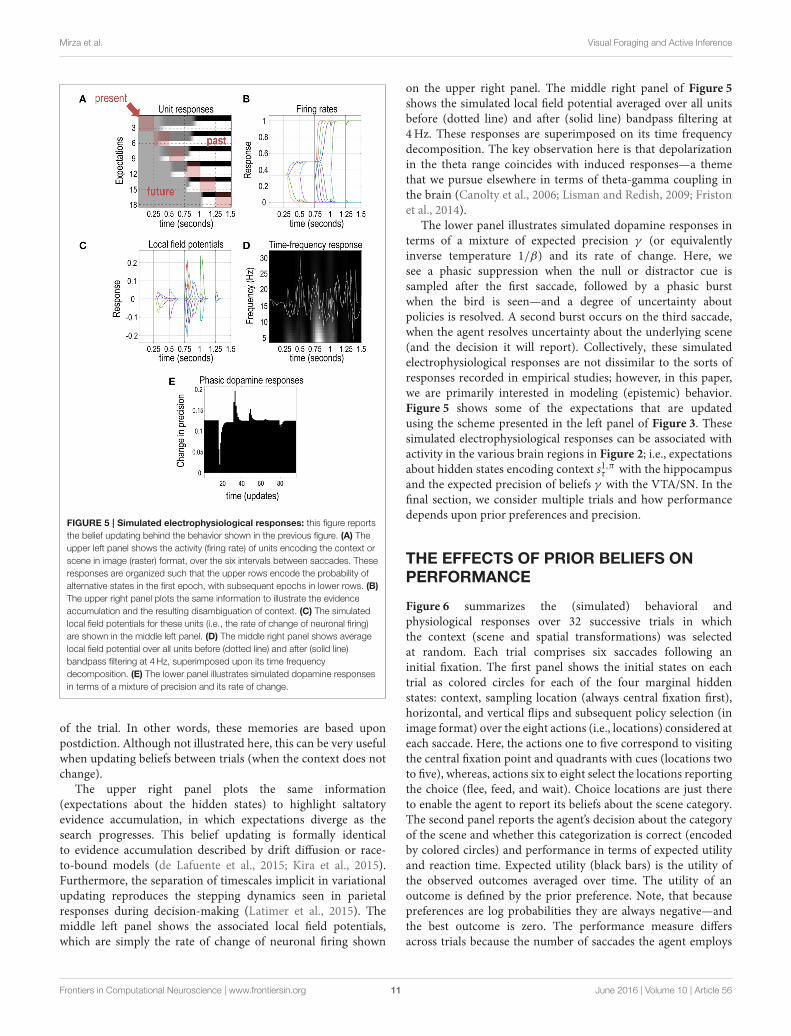
FIGURE 5 | Simulated electrophysiological responses: this figure reports

the belief updating behind the behavior shown in the previous figure. (A) The

upper left panel shows the activity (firing rate) of units encoding the context or

scene in image (raster) format, over the six intervals between saccades. These

responses are organized such that the upper rows encode the probability of

alternative states in the first epoch, with subsequent epochs in lower rows. (B)

The upper right panel plots the same information to illustrate the evidence

accumulation and the resulting disambiguation of context. (C) The simulated

local field potentials for these units (i.e., the rate of change of neuronal firing)

are shown in the middle left panel. (D) The middle right panel shows average

local field potential over all units before (dotted line) and after (solid line)

bandpass filtering at 4Hz, superimposed upon its time frequency

decomposition. (E) The lower panel illustrates simulated dopamine responses

in terms of a mixture of precision and its rate of change.

of the trial. In other words, these memories are based uponpostdiction. Although not illustrated here, this can be very usefulwhen updating beliefs between trials (when the context does notchange).

The upper right panel plots the same information(expectations about the hidden states) to highlight saltatoryevidence accumulation, in which expectations diverge as thesearch progresses. This belief updating is formally identicalto evidence accumulation described by drift diffusion or race-to-bound models (de Lafuente et al., 2015; Kira et al., 2015).Furthermore, the separation of timescales implicit in variationalupdating reproduces the stepping dynamics seen in parietalresponses during decision-making (Latimer et al., 2015). Themiddle left panel shows the associated local field potentials,which are simply the rate of change of neuronal firing shown

on the upper right panel. The middle right panel of Figure 5shows the simulated local field potential averaged over all unitsbefore (dotted line) and after (solid line) bandpass filtering at4Hz. These responses are superimposed on its time frequencydecomposition. The key observation here is that depolarizationin the theta range coincides with induced responses—a themethat we pursue elsewhere in terms of theta-gamma coupling inthe brain (Canolty et al., 2006; Lisman and Redish, 2009; Fristonet al., 2014).

The lower panel illustrates simulated dopamine responses interms of a mixture of expected precision γ (or equivalentlyinverse temperature 1/β) and its rate of change. Here, wesee a phasic suppression when the null or distractor cue issampled after the first saccade, followed by a phasic burstwhen the bird is seen—and a degree of uncertainty aboutpolicies is resolved. A second burst occurs on the third saccade,when the agent resolves uncertainty about the underlying scene(and the decision it will report). Collectively, these simulatedelectrophysiological responses are not dissimilar to the sorts ofresponses recorded in empirical studies; however, in this paper,we are primarily interested in modeling (epistemic) behavior.Figure 5 shows some of the expectations that are updatedusing the scheme presented in the left panel of Figure 3. Thesesimulated electrophysiological responses can be associated withactivity in the various brain regions in Figure 2; i.e., expectationsabout hidden states encoding context s1,πτ with the hippocampusand the expected precision of beliefs γ with the VTA/SN. In thefinal section, we consider multiple trials and how performancedepends upon prior preferences and precision.

THE EFFECTS OF PRIOR BELIEFS ONPERFORMANCE

Figure 6 summarizes the (simulated) behavioral andphysiological responses over 32 successive trials in whichthe context (scene and spatial transformations) was selectedat random. Each trial comprises six saccades following aninitial fixation. The first panel shows the initial states on eachtrial as colored circles for each of the four marginal hiddenstates: context, sampling location (always central fixation first),horizontal, and vertical flips and subsequent policy selection (inimage format) over the eight actions (i.e., locations) considered ateach saccade. Here, the actions one to five correspond to visitingthe central fixation point and quadrants with cues (locations twoto five), whereas, actions six to eight select the locations reportingthe choice (flee, feed, and wait). Choice locations are just thereto enable the agent to report its beliefs about the scene category.The second panel reports the agent’s decision about the categoryof the scene and whether this categorization is correct (encodedby colored circles) and performance in terms of expected utilityand reaction time. Expected utility (black bars) is the utility ofthe observed outcomes averaged over time. The utility of anoutcome is defined by the prior preference. Note, that becausepreferences are log probabilities they are always negative—andthe best outcome is zero. The performance measure differsacross trials because the number of saccades the agent employs






FIGURE 6 | Simulated responses over 32 trials: this figure reports the behavioral and (simulated) physiological responses during 32 successive trials. The scenes

in these 32 trials were specified via randomly selected hidden states of the world. (A) The first panel shows the hidden states of the scene (as colored circles) and the

selected action (i.e., the sampled location) on the last saccade. The y-axis on this panel shows two quantities. The selected action is shown using black bars. The

agent can saccade to locations one to eight, where the locations six to eight correspond to the choice locations the agent uses to report the scene category. The true

hidden states are shown with colored circles. These specify the objects in the scene and their locations (in terms of the context and spatial transformations). The

second row of cyan dots indicates that the agent always starts exploring a scene from the central fixation point. Individual rows in the y-axis indicate the sampled

locations according to the following: Fix, Fixation; U. Left, Upper left; L. Left, Lower Left; U. Right, Upper Right; L. Right, Lower Right; and Ch. Flee, Choose Flee; Ch.

Feed, Choose Feed; and Ch. Wait, Choose Wait. (B) The second panel reports the final outcomes (encoded by colored circles) and performance measures in terms of

preferred outcomes (utility of observed outcomes), summed over time (black bars) and standardized reaction times (cyan dots). The final outcomes are shown for the

sample location (upper row of dots) and outcome (lower row of dots): yellow means the agent made a right choice. (C) The third panel shows a succession of

simulated event related potentials following each outcome. These are taken to be the rate of change of neuronal activity, encoding the expected probability of hidden

states encoding context (i.e., simulated hippocampal activity).

before categorizing a scene differs from trial to trial. The reactiontimes or saccadic intervals (cyan dots) here are based upon theactual processing time in the simulations and are shown afternormalization to a mean of zero and standard deviation of one.Our definition of reaction time as the actual processing time(using Matlab tic-toc facility) in the simulations is based uponthe assumption that belief updates in the brain—via neuronalmessage passing—follow a similar scheduling to the exchange ofsufficient statistics described in Figure 3.

These simulations show that, with the exception of the thirdtrial, the agent makes veridical decisions on every occasion.Interestingly, the third (incorrect) trial is associated with thegreatest reaction time. Reaction time here varies because theminimization of free energy converges at a certain tolerance(here, the variational updates terminate when the decrease in freeenergy falls below 1/128). The lower panel shows the simulatedelectrophysiological responses using the same format as in theprevious figure. Here, we see bursts of high-frequency activity

every 100ms or so; in other words, a nesting of gamma activityin the alpha range.

The associated behavior, over the first nine trials is depictedin Figure 7. Again, with the exception of the third trial, we seeoptimal search behavior, with a correct choice after the minimumnumber of saccades. For example, on the first trial, the firstsaccade samples a bird, which just requires a second saccade tothe adjacent location in order to completely disambiguate thecontext. A detailed analysis of the belief updating for the failedtrial suggested that this was an unlucky failure of the meanfield approximation; particularly the factorization over time—and a partial failure of convergence due to the use of a fixednumber (i.e., 16) of iterations. These sorts of failures highlight thedistinction between exact Bayesian inference and approximateBayesian inference that may underlie bounded rationality in realagents. With these simulated responses is at hand, we can nowassess the effects of changing prior preference and priors over theprecision of beliefs about action or policies.






FIGURE 7 | Sequences of saccades: this figure illustrates the behavior for

the first nine trials shown in the previous figure using the same format as

Figure 4 (upper right panel). The numbers on the top left in each cell show the

trial number. With the exception of the third trial, the agent is able to recognize

or categorize the scene after a small number of epistemically efficient

saccades.

Clearly, there are many model parameters (andhyperparameters) we could consider, in terms of their effects onsimulated behavior. We focused on the precision of preferencesand policies because these correspond intuitively to the differentaspects of salience that may be aberrant in schizophrenia.Motivational salience can be associated with the preferencesthat incentivise choice behavior. Conversely, the precision ofbeliefs about policies speaks to the visual salience associated withinformation gain and epistemic value. Heuristically, one mightexpect different patterns of behavior depending upon whethersubjects have imprecise preferences (i.e., are not confidentabout what to do), as opposed to imprecise beliefs about theconsequences of their actions (i.e., not confident about how todo it). In what follows, we address this heuristic using simulatedbehavior.

The Effect of PriorsFinally, Figure 8 reports the performance during presentationsof 300 trials, where hidden states of the world were selectedrandomly—and we allowed the agent to make up to 8 saccades.We measured the performance over these trials in termsof percent accuracy (a correct choice in the absence of an

incorrect choice), decision time or number of saccades untilany (correct or incorrect) choice and reaction time or saccadicinterval (measured in seconds). Here, we repeated the 300 trialparadigm over all combinations of eight levels of prior preferenceand precision. To manipulate the precision of preferences, weincreased the parameter c—specifying the prior preferences fordifferent outcomes—from 0 to 4 (i.e., no preferences to veryprecise preferences).

The left panel in Figure 8 (Accuracy) shows that accuratecategorization requires both precise preferences and a highprecision. Interestingly, precise prior preferences degradeaccuracy when the prior precision is very low. With greaterprior preference, the agent does not want to make mistakes.However, a low prior precision precludes a resolution ofuncertainty about the scene. The combination of these two priorsdiscourages the agent from making a choice, resulting in anincorrect categorization. The trials where agent doesn’t attemptto categorize the scene are considered an incorrect categorization.When prior preferences are less precise, the agent is less afraidof making an incorrect choice, resulting in an improvementin performance but it is still below the chance level. Similarly,greater prior precision does not improve accuracy when priorpreference is low. In short, the agent only respond accuratelywhen prior preference and precision are high, as seen on theupper right portion of the image.

The center panel (Decision Time) shows decision time interms of number of saccades before choosing a choice location.When prior preferences are high and prior precision is very low(first column), it takes seven or eight saccades for the agent tomake a decision. Comparing this figure with the accuracy results,it can be seen that accuracy is low even though the agent ismaking more saccades; i.e., taking its time. When prior precisionis high but prior preference is very low, the agent rushes to makea decision—but in the absence of precise prior preferences itmakes mistakes (see left panel). In short, the agent successfullycategorizes a scene when it deploys three to four saccades (upperright quadrants), under precise preferences and high precision.

The right panel (Reaction Time) shows the reaction time interms of actual processing time of the simulations. Although,quantitatively, reaction times only vary between about 800 and900ms, there seems to be a systematic effect of prior precision,with an increase in reaction time at very low levels.

Crucially, results demonstrate a distinct dependency ofaccuracy and decision time on prior preference and priorprecision. This speaks to the possibility of distinct behavioralphenotypes that are characterized by different combinationsof prior preference and precision. For example, agents whodo not expect themselves to make mistakes may choosemore assiduously, inducing a classical speed accuracy trade-off.Conversely, subjects with more precise beliefs about their choicesmay behave in a more purposeful and deliberate fashion, takingless time to obtain preferred outcomes. We pursue this theme inthe discussion.

DISCUSSION

In summary, we have presented an active inference formulationof epistemic foraging that provides a framework for






FIGURE 8 | Performance and priors: this figure illustrates the average performance over 300 trials. (A) The insert (lower panel) shows the prior parameters that

were varied; namely, prior preference and precision. These parameters are varied over eight levels. (B) For each combination, the accuracy, decision and reaction time

were evaluated using simulations (upper row). The accuracy is expressed as the percentage of correct trials (defined as a correct choice in the absence of a

proceeding or subsequent incorrect choice). Decision time is defined in terms of the number of saccades until a (correct or incorrect) decision. Reaction time or the

interval between saccades is measured in seconds and corresponds to the actual computation time during the simulations.

understanding the functional anatomy of visual search entailedby sequences of saccadic eye movements. This formulationprovides an elementary solution to the problem of sceneconstruction in the context of active sensing and sequentialpolicy optimization, while incidentally furnishing a model ofspatial invariance in vision.

Although the problem considered above is relatively simple,it would confound most existing approaches. For example,reinforcement learning and optimal control theories are notapplicable because the problem is quintessentially epistemic(belief-based) in nature. This means that the optimal actiondepends on beliefs or uncertainty about hidden states. Thiscontext sensitivity precludes any state-action policy andimplicitly any scheme based on the Bellman optimality principle(Bellman, 1952). This is because the optimal action from anystate depends upon beliefs about that state and all others.Although, in principle, a belief-state (partially observed) Markovdecision process could be entertained (Bonet and Geffner,2014), the combinatorics of formulating beliefs states over3 × 8 × 2 × 2 = 96 hidden states are daunting. Furthermore,given the problem calls for sequential policy optimization—and that five moves are necessary to guarantee a correctcategorization—one would have to evaluate 85 = 32768policies.

The active inference solution offered here is based uponminimizing the path-integral of (expected) free energy undera mean field approximation. The exciting thing about thisapproach is that, computationally, it operates (nearly) in real-time. For example, the reaction times in Figure 8 are basedon the actual computation time using a standard desktoppersonal computer. This computational efficiency may be usefulfor neurorobotic applications. Having said this, the primarymotivation for developing this scheme was to characterizeempirical (human) visual searches given observed performance,eye movement, and electrophysiological responses.

The example in this paper has some limitations: for example,all potential spatial combinations of objects can be obtained usingjust two transformations (e.g., the cat can never be below thebird), and scenes in larger grid worlds may not be describable interms of simple transformations from a small number of contexts.Clearly, the brain does not use the mean field approximationused to illustrate the scheme—but questions about differentforms of meaningful approximations can, in principle, beanswered empirically using Bayesian model comparison of suchapproximations when explaining behavioral or neuroimagingdata.

This toy example shows how a scene comprising 2 × 2quadrants can be explored using the resolution of uncertainty.






A scene of this small size could be explored systematically, ifinefficiently, (e.g., in a clockwise manner) or by just visiting alllocations randomly. However, more complex scenes—which wehope to use in future work—could not be categorized efficientlyin such a fashion. In future work, we intend to expand thescene in terms of its size and contents, while retaining thesame (active inference) formulation of exploration and ensuingcategorization. Our hope is to characterize different behavioralphenotypes, defined in terms of the free parameters of this model;namely, the prior preferences and precision. This paradigm willbe used to test the aberrant salience hypothesis of schizophrenia.For that purpose, the experimental design will include taskirrelevant distractors (as opposed to the null cues used above),probabilistic relationships between the contents of the scene andits category—and a greater number of cue locations. In principle,this will allow us to explain the difference between normal andschizotypal visual searches in terms of prior preferences, priorprecision or a mixture of the two.

Although the accuracy, number of saccades and saccadicintervals (Figure 8) provide a degree of validation for activeinference in this setting, it is unlikely that these responses willprovide an efficient estimate of subject-specific priors, such asprior preferences and precision. However, it is relatively easyto fit the individual saccadic eye movements by evaluating theprobability of each saccade in relation to posterior beliefs aboutaction, using the history of action and outcomes in the modelabove. This means, in principle, it should be possible to estimate

things like prior preference and precision efficiently, given thesequence of eye movements from any subject. In subsequentwork, we will use the active inference scheme described inthis paper to explain empirical eye movements in terms ofsubject-specific priors. This enables one to simulate or modelelectrophysiological responses or identify the regional correlatesof belief updating, using functional magnetic resonanceimaging. This speaks to the ultimate aim of this work, whichis to provide a computational phenotyping of individuals, inthe hope of characterizing the (formal or computational)psychopathology of conditions like addiction andschizophrenia.

AUTHOR CONTRIBUTIONS

MM, CM, RA conceived the idea. KF, MM, RA, CM contributedto the writing. KF, MM conducted the simulations.

FUNDING

MM, RA, and KF are members of PACE (Perception andAction in Complex Environments), an Innovative TrainingNetwork funded by the European Union’s Horizon 2020 researchand innovation programme under the Marie-Sklodowska-CurieGrant Agreement No 642961. CM is funded by the MaxPlanck Society. KF is funded by the Wellcome trust (Ref:088130/Z/09/Z).

REFERENCES

Andreopoulos, A., and Tsotsos, J. (2013). A computational learning theory of active

object recognition under uncertainty. Int. J. Comput. Vis. 101, 95–142. doi:

10.1007/s11263-012-0551-6

Barlow, H. (1961). “Possible principles underlying the transformations of sensory

messages,” in Sensory Communication, edW. Rosenblith (Cambridge,MA:MIT

Press), 217–234.

Beal, M. J. (2003). Variational Algorithms for Approximate Bayesian Inference.

Ph.D. thesis, University College London.

Beedie, S. A., Benson, P. J., and St Clair, D. M. (2011). Atypical scanpaths

in schizophrenia: evidence of a trait- or state-dependent phenomenon?

J. Psychiatry Neurosci. 36, 150–164. doi: 10.1503/jpn.090169

Bellman, R. (1952). On the theory of dynamic programming. Proc. Natl. Acad. Sci.

U.S.A 38, 716–719.

Bonet, B., and Geffner, H. (2014). Belief tracking for planning with sensing: width,

complexity and approximations. J. Artif. Intell. Res. 50, 923–970. doi: 10.1613/

jair.4475

Braun, D. A., Ortega, P. A., Theodorou, E., and Schaal, S. (2011). “Path integral

control and bounded rationality,” in 2011 IEEE Symposium on Adaptive

Dynamic Programming and Reinforcement Learning (ADPRL) (Paris: IEEE).

Canolty, R. T., Edwards, E., Dalal, S. S., Soltani, M., Nagarajan, S. S., Kirsch, H. E.,

et al. (2006). High gamma power is phase-locked to theta oscillations in human

neocortex. Science 313, 1626–1628. doi: 10.1126/science.1128115

de Lafuente, V., Jazayeri, M., and Shadlen, M. N. (2015). Representation of

accumulating evidence for a decision in two parietal areas. J. Neurosci. 35,

4306–4318. doi: 10.1523/JNEUROSCI.2451-14.2015

Donaldson, I. M. (2000). The functions of the proprioceptors of the eye muscles.

Philos. Trans. R. Soc. B Biol. Sci. 355, 1685–1754. doi: 10.1098/rstb.2000.0732

Duhamel, J. R., Colby, C. L., and Goldberg, M. E. (1992). The updating of the

representation of visual space in parietal cortex by intended eye movements

Science 255, 90–92. doi: 10.1126/science.1553535

FitzGerald, T. H., Schwartenbeck, P., Moutoussis, M., Dolan, R. J., and Friston,

K. (2015). Active inference, evidence accumulation, and the urn task. Neural

Comput. 27, 306–328. doi: 10.1162/NECO_a_00699

Frank, M. J. (2011). Computational models of motivated action selection

in corticostriatal circuits. Curr. Opin. Neurobiol. 21, 381–386 doi:

10.1016/j.conb.2011.02.013

Friston, K., Adams, R. A., Perrinet, L., and Breakspear, M. (2012). Perceptions

as hypotheses: saccades as experiments. Front. Psychol. 3:151. doi:

10.3389/fpsyg.2012.0015

Friston, K., Mattout, J., and Kilner, J. (2011). Action understanding and active

inference. Biol. Cybern. 104, 137–160. doi: 10.1007/s00422-011-0424-z

Friston, K., Rigoli, F., Ognibene, D., Mathys, C., Fitzgerald, T., and Pezzulo, G.

(2015). Active inference and epistemic value. Cogn Neurosci. 6, 187–214. doi:

10.1080/17588928.2015.1020053

Friston, K., Schwartenbeck, P., FitzGerald, T., Moutoussis, M., Behrens, T., and

Dolan, R. J. (2014). The anatomy of choice: dopamine and decision-making.

Philos. Trans. R. Soc. Lond. B Biol. Sci. 369:20130481. doi: 10.1098/rstb.2013.

0481

Friston, K., Schwartenbeck, P., FitzGerald, T., Moutoussis, M., Behrens, T., and

Raymond Dolan, R. J. J. (2013). The anatomy of choice: active inference and

agency. Front. Hum. Neurosci. 7:598. doi: 10.3389/fnhum.2013.00598

Grossberg, S., Roberts, K., Aguilar, M., and Bullock, D. (1997). A neural model

of multimodal adaptive saccadic eye movement control by superior colliculus.

J. Neurosci. 17, 9706–9725.

Hassabis, D., and Maguire, E. A. (2007). Deconstructing episodic memory with

construction. Trends Cogn. Sci. 11, 299–306. doi: 10.1016/j.tics.2007.05.001

Haxby, J. V., Horwitz, B., Ungerleider, L. G., Maisog, J. M., Pietrini, P., and

Grady, C. L. (1994). The functional organization of human extrastriate cortex:

a PET-rCBF study of selective attention to faces and locations. J. Neurosci. 14,

6336–6353

Howard, R. (1966). Information value theory. IEEE Trans. Syst. Sci. Cybern. 2,

22–26. doi: 10.1109/TSSC.1966.300074






Itti, L., and Baldi, P. (2009). Bayesian surprise attracts human attention. Vision Res.

49, 1295–1306. doi: 10.1016/j.visres.2008.09.007

Jaakkola, T., and Jordan, M. (1998). “Improving the mean field approximation via

the use of mixture distributions,” in Learning in Graphical Models, Vol. 89, ed

M. Jordan, (Netherlands: Springer), 163–173.

Kapur, S. (2003). Psychosis as a state of aberrant salience: a framework

linking biology, phenomenology, and pharmacology in schizophrenia. Am. J.

Psychiatry 160, 13–23. doi: 10.1176/appi.ajp.160.1.13

Kira, S., Yang, T., and Shadlen, M. N. (2015). A neural implementation

of Wald’s sequential probability ratio test. Neuron 85, 861–873. doi:

10.1016/j.neuron.2015.01.007

Klyubin, A. S., Polani, D., and Nehaniv, C. L. (2005). “Empowerment: a universal

agent-centric measure of control,” in Proc. CEC 2005, Vol. 1 (Edinburgh: IEEE),

128–135.

Latimer, K. W., Yates, J. L., Meister, M. L., Huk, A. C., and Pillow, J. W.

(2015). NEURONAL MODELING. Single-trial spike trains in parietal cortex

reveal discrete steps during decision-making. Science 349, 184–187. doi:

10.1126/science.aaa4056

Laughlin, S. B. (2001). Efficiency and complexity in neural coding.Novartis Found.

Symp. 239, 177–187. doi: 10.1002/0470846674.ch14

Linsker, R. (1990). Perceptual neural organization: some approaches based on

network models and information theory. Annu. Rev. Neurosci. 13, 257–281.

Lisman, J., and Redish, A. D. (2009). Prediction, sequences and the

hippocampus. Philos. Trans. R. Soc. Lond. B Biol. Sci. 364, 1193–1201.

doi: 10.1098/rstb.2008.0316

Moutoussis, M., Trujillo-Barreto, N. J., El-Deredy, W., Dolan, R. J., and Friston,

K. J. (2014). A formal model of interpersonal inference. Front. Hum. Neurosci.

8:160. doi: 10.3389/fnhum.2014.00160

Olshausen, B. A., and Field, D. J. (1996). Emergence of simple-cell receptive field

properties by learning a sparse code for natural images. Nature 381, 607–609.

Ortega, P. A., and Braun, D. A. (2013). Thermodynamics as a theory of decision-

making with information-processing costs. Proc. R. Soc. A 469, 2153. doi:

10.1098/rspa.2012.0683

Pezzulo, G., Rigoli, F., and Chersi, F. (2013). The mixed instrumental

controller: using value of information to combine habitual choice

and mental simulation. Front. Psychol. 4:92. doi: 10.3389/fpsyg.2013.

00092

Rudy, J. W. (2009). Context representations, context functions, and the

parahippocampal-hippocampal system. Learn. Mem. 16, 573–585. doi:

10.1101/lm.1494409

Schmidhuber, J. (1991). “Curious model-building control systems,” in Proc.

International Joint Conference on Neural Networks, Vol. 2, (Singapore: IEEE),

1458–1463.

Schultz, W., Dayan, P., and Montague, P. R. (1997). A neural

substrate of prediction and reward. Science 275, 1593–1599. doi:

10.1126/science.275.5306.1593

Schwartenbeck, P., FitzGerald, T. H., Mathys, C., Dolan, R., and Friston, K. (2014).

The dopaminergic midbrain encodes the expected certainty about desired

outcomes. Cereb. Cortex 25, 3434–3445. doi: 10.1093/cercor/bhu159

Schwartenbeck, P., FitzGerald, T. H., Mathys, C., Dolan, R., Wurst, F.,

Kronbichler, M., et al. (2015). Optimal inference with suboptimal models:

addiction and active Bayesian inference. Med. Hypotheses 84, 109–117. doi:

10.1016/j.mehy.2014.12.007

Seeck, M., Schomer, D., Mainwaring, N., Ives, J., Dubuisson, D., Blume, H., et al.

(1995). Selectively distributed processing of visual object recognition in the

temporal and frontal lobes of the human brain. Ann. Neurol. 37, 538–545. doi:

10.1002/ana.410370417

Shen, K., Valero, J., Day, G. S., and Paré, M. (2011). Investigating the role of the

superior colliculus in active vision with the visual search paradigm. Eur. J.

Neurosci. 33, 2003–2016. doi: 10.1111/j.1460-9568.2011.07722.x

Srihasam, K., Bullock, D., and Grossberg, S. (2009). Target selection by the

frontal cortex during coordinated saccadic and smooth pursuit eye movements.

J. Cogn. Neurosci. 21, 1611–1627. doi: 10.1162/jocn.2009.21139

Still, S., and Precup, D. (2012). An information-theoretic approach to

curiosity-driven reinforcement learning. Theory Biosci. 131, 139–148. doi:

10.1007/s12064-011-0142-z

Tanji, J., and Hoshi, E. (2001). Behavioral planning in the prefrontal cortex Curr.

Opin. Neurobiol. 11, 164–170 doi: 10.1016/S0959-4388(00)00192-6

Ungerleider, L. G., and Mishkin, M. (1982). “Two cortical visual systems,” in

Analysis of Visual Behavior, eds D. Ingle, M. A. Goodale, and R. J. W. Mansfield

(Cambridge, MA: MIT Press), 549–586.

van den Broek, J. L.,Wiegerinck,W. A. J. J., and Kappen, H. J. (2010). Risk-sensitive

path integral control. UAI 6, 1–8.

Wurtz, R. H., McAlonan, K., Cavanaugh, J., and Berman, R. A. (2011).

Thalamic pathways for active vision. Trends Cogn. Sci. 5, 177–184. doi:

10.1016/j.tics.2011.02.004

Zeidman, P., Lutti, A., and Maguire, E. A. (2015). Investigating the functions

of subregions within anterior hippocampus. Cortex 73, 240–256. doi:

10.1016/j.cortex.2015.09.002

Zeki, S., and Shipp, S. (1988). The functional logic of cortical connections. Nature

335, 311–317.

Conflict of Interest Statement: The authors declare that the research was

conducted in the absence of any commercial or financial relationships that could

be construed as a potential conflict of interest.

Copyright © 2016 Mirza, Adams, Mathys and Friston. This is an open-access article

distributed under the terms of the Creative Commons Attribution License (CC BY).

The use, distribution or reproduction in other forums is permitted, provided the

original author(s) or licensor are credited and that the original publication in this

journal is cited, in accordance with accepted academic practice. No use, distribution

or reproduction is permitted which does not comply with these terms.


http://creativecommons.org/licenses/by/4.0/








Documents

Scene Construction, Visual Foraging, and Active Inferencekarl/Scene... · Mirza et al. Visual Foraging and Active Inference. the assumption that action and perception serve to minimize