Scene Classification in Images

B V V Sri Raj Dutt Pulkit Agrawal Sushoban Nayak

Abstract

In this paper, following the works of Oliva and Torralba, we present a procedure to classify realworld scenes in eight semantic groups of coast, forest, mountain, open country, street, tall building,highway and inside city, without going through the stages of segmentation and processing of individ-ual objects or regions. The approach essentially takes into account the diagonistic information stored inthe power spectrum of each category of images and through supervised learning, separates character-istic feature vectors of each class in separate groups that helps assign a new test image to its respectivegroup. We follow a sequential hierarchy in which images are first sorted according to their natural-ness and through traversing a tree, we ultimately reach the desired node that represents the class of theimage. The significance of results obtained and the ripple effect of errors have also been reflected upon.

Keywords: scene classification, Gabor filter, LDA

1 Introduction

The statement ”Machines shall rule the world” is no more a mere figment of imagination, for its thepromise of Machine learning. In our quest to design and manufacture robotic replicates of humans wehaven’t come a long way, yet we have with us a set of techniques, algorithms and models which serve as agood starting point. The mystery of how human brain functions has evaded researchers for centuries.Theaim of research has been to empower our mechanical creations to think and analyze situations in wayssimilar to us. In fact, modelling the human brain and realizing it physically is the greatest challenge of thecentury.

Artificial Intelligence combines work in fields like computer science, neuroscience, mathematics, psy-chology, philosophy, cognitive sciences etc. Also, often progress is made by simultaneous contributionsfrom more than one areas. For example, advances in cognitive psychology have led us to believe that ourbrain processes information in a top-down” manner rather than doing it in a bottom-up” manner. It hasalso been proposed that the brain develops models and templates for information it encounters, i.e., it has amodel for a building, for a game of cricket, for the music of guitar, and so on for almost everything whichwe can observe and feel. In case it encounters something new it tries to correlate to something it alreadyknows and at times it can form a new model as well. Moreover these models and conceptions of thingskeep evolving with time and with our interaction with environment.Capturing this mammoth collection ofmodels,concepts and information in a machine is a very big challenge.

One of the main features of our daily experience is the ability to distinguish between things , to identifythem and to link them with our prior knowledge. This ability to recognize and interpret the environment

1

around us, is in principle the foundation for any higher level of processing that we do. Synonymous is theconcept of clustering, segmentation and classification in artificial intelligence.Inspired by the working ofhuman brain, the conception of learning algorithms took birth. These algorithms in essence provide us witha methodology to find parameters which would be able to identify and classify different objects in a givensignal input.Researchers, in general have looked at different aspects of the brain like vision,hearing,speechetc for a better understanding of their functioning and in an attempt to model these processes.

We consider here a fundamental problem of computer vision, i.e. enabling computers to see the waywe see things. We in future wish our machines would match the capabilities of human vision.Its interest-ing to note that, every second we receive tremendous amount of visual data and almost unconsciously weprocess this information very quickly. Classifying an object as table, a ball, or a scene as mountain or riveris pretty trivial for us. We can in fact process amazingly more complex information. Its a well known factthat robotic vision compares miserably with our eyes.Here, we intend to make a start towards our goal byconsidering a very trivial problem by the standard of human vision and that is scene classification. Givenan image of the scene we wish to classify it as say a mountain, forest, city, street etc.

Generally, a learning based approach is used to solve problems of this nature. A training set is initiallycreated which would contain representative images from all categories that we need to classify. Now theseimages are manually labeled to the class they belong as perceived by the human. Now a learning algo-rithm is employed, which basically is a strategy to enable us to come up with parameters which wouldcharacterize an image for doing the classification task. Now if a random image is given as an input, onbasis of parameters already identified the machine would try to classify the image. This in essence id ageneric way in which learning algorithms work, i.e., by learning from a huge set of data and then usingthis learned information to make predictions about successive inputs.

2 Introduction

2.1 What is a scene ?

Our project mainly focuses on classifying scene and as such it’s imperative that we clarify what we meanby a scene. To distinguish scene from ’object’ or ’texture’, we follow the approach taken by [5] and weconsider the absolute distance between observer and the fixated zone as the discriminating factor. So, an’object’ is something that subtends about 1 to 2 meters around the observer; but in case of a scene, thedistance between the observer and the fixated point is usually more than 5 meters. To put it in commonterms, object is something that is at hand distance whereas scene is mainly a place in which one can move.

2.2 Scene Recognition

Following the approach of the experimental schools, for whom recognition of scene means providinginformation about the semantic category and the function of the environment, we propose a computa-tional model of recognition of scene categories. There are fundamentally two types of scene recognitiontechniques found in literature. The first one is the bottom up approach of employing object recognition

2

to decide the category of the scene. We here follow the second approach that essentially is a top-downapproach. We bypass segmentation and processing of objects and try to categorize each scene throughassimilating its global information. The reason we go for the second approach is that it is supported bypsychological experiments, which propose that humans accumulate enough information about the mean-ing of a scene in less than 200ms, which can only mean that we go for an overview rather than a detailedanalysis of object and texture. Especially while dealing with environmental pictures, object informationis spontaneously ignored. For example, [3] confirms that coarse blobs made of spatial frequency as lowas 4 to 8 cycles per image provided enough information for instant recognition of common environmentseven when the shape and identity of objects could not be recovered. Some other studies have also shownthat people can be totally blind to object changes, even when they are meaningful part of the scene ([5]).So effectively, at a first glance, we just assimilate the gist of an image which is built on a low resolutionspatial configuration.

2.3 Defining the Problem:

Given an image as an input we wish to classify as one of the following:

1. Coast

2. Forest

3. Highway

4. Inside City

5. Mountain

6. Open Country

7. Street

8. Tall Buildings

The image classes are standard image classes which have been used extensively in research to date.We have used the Oliva Toralba dataset which is a subset of the Corel database for our project. Somerepresentative images from the image data set have been shown in the section 4.

3 History

There are many ways in which previous works have approached this problem. [4] uses the traditionalidea of bottom up approach where scene recognition is done through segmentation of image into regionsinstead of going for global features. [10] goes for a typicality approach. [8] eliminates the need for human-annotations of image features. [2] introduces the concept of recognizing scenes on approximate globalgeometric correspondence and claims to get high recognition rates on challenging data. [6] emphasizes thefact that we recognize images at different scales and not just with global features or only with local featuresand does a very good work of classifying images. However, given the time and resources available, and

3

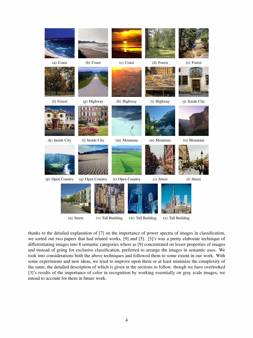
(a) Coast (b) Coast (c) Coast (d) Forest (e) Forest

(f) Forest (g) Highway (h) Highway (i) Highway (j) Inside City

(k) Inside City (l) Inside City (m) Mountain (n) Mountain (o) Mountain

(p) Open Country (q) Open Country (r) Open Country (s) Street (t) Street

(u) Street (v) Tall Building (w) Tall Building (x) Tall Building

thanks to the detailed explanation of [7] on the importance of power spectra of images in classification,we sorted out two papers that had related works, [9] and [5]. [5]’s was a pretty elaborate technique ofdifferentiating images into 8 semantic categories where as [9] concentrated on lesser properties of imagesand instead of going for exclusive classification, preferred to arrange the images in semantic axes. Wetook into considerations both the above techniques and followed them to some extent in our work. Withsome experiments and new ideas, we tried to improve upon them or at least minimize the complexity ofthe same, the detailed description of which is given in the sections to follow. though we have overlooked[3]’s results of the importance of color in recognition by working essentially on gray scale images, weintend to account for them in future work.

4

4 Dataset

Some of the images from the dataset have been shown in the figure.

Some Notes :

• Open country is essentially the countryside.

• Tall Buildings includes skylines and sky scrapers where as Inside city is a photo a characteristic cityscene generally without the skyline.

5 Our work

5.1 What are we on a look out for ?

We essentially need to figure out features such that Image = f(features). The most important characteristicof feature that we require is a very strong co-relation between the feature value and the class of the image.This makes learning an easier, faster and a less error prone job. Thus, feature identification is amongthe most important task. Once, the features are identified a classifier can be constructed using state ofart algorithms like SVM’s, k-means, Bayes method, Linear discriminant analysis or any other suitablemethod. With help of this classifier, identification of an input image needs to be done.

Basic Approach towards classification : On the basis of psychological experiments, some propertiescapturing the most important aspects of a scene were identified( [1]). In the same work, they tried express-ing as a function of these properties like naturalness, openness etc. With this work as the background, wedecided to form a tree classifier of the structure of one shown in (Fig). Firstly, the image is classified asArtificial or Natural. Next an artificial image is classified into 2 groups, (street and highway) or (insidecity and tall buildings) and in the next step these groups are classified into their constituent classes. Thisclassification was done on an intuitive basis. For example, street and highway show similar characteristics,so do open country and coast (both have horizons and are open in some sense). Some different combina-tions of grouping were tried like clubbing street and tall buildings together (as buildings are often presenton the side of the street) etc. A more rigorous approach towards formation of tree structured classifier wasnot used as results with some combinations we worked were not significantly different. This is discussedin more details in scope of future work.

5.2 Things we tried :

• Haar features : Motivation : Fast and is known to work well in image processing tasks such as facedetection. We divided the image into blocks of sizes 64*64 and in each block applied Harr transformsuccessively 2 times to get the LL component of each block. Then the combined set of these LLfeatures of each block was considered in the set of feature vector corresponding to the image. Whilecalculating the distinguishing weights for features from LDA, the matrix was nearly singular andsolution of SVM did not converge and hence we had to abandon this approach. The results obtainedfrom LDA inspite of the near singularity of matrix have been shown in the figure.

5

Figure 1: Distribution obtained when using Harr features

• Edges : Motivation : Edges can give a rough idea of the scene. Tall buildings for example wouldshow many long vertical edges and possibly numerous horizontal edges, similarly a forest wouldshow uniform distribution of dominant long vertical edges (presence of trees). Coast and opencountry on the hand would give a relatively fewer edges and more of horizontal lines as prominentones (owing to the horizon etc). Mountains on the other hand can be expected to give more ofdiagonal edges, due to their characteristic shape, similarly streets and highways have characteristicedges marking the outlines of the road. The results we have obtained on finding edges for differentcategories of images are given in Appendix 1.

Comparing the edge maps of various images, we found loads of noise in the edges making it torather difficult to identify features. Thus this method was discarded without any further analysis.

• Colour Features: We asked ourselves a basic question, is it possible to classify the images onlybased on the colour information ??

Motivation :

We were motivated by the fact that colours provide an important clue towards discerning the image.A coast for example would have a large span of blue region, mountains, forest, open country wouldshow a lot of green, highways and streets would contain a gray path like region in the middle of theimage, tall buildings would have a skyline(blue in general) other than the colour cues from coloursof buildings (which are very different from colours of natural images).

Formation of feature vector :

– Image is resized to 256*256 using bilinear interpolation.

– Image is divided into blocks of 64*64.

– The mean of ’Red’, ’Green’ and ’Blue’ colour values are individually calculated for each blockand are used as features.

– Thus we have a feature vector of size : NumberOfBlocks∗3 ∗ 1 = 768 features.

– Now we find a discriminant vector for each division as we go down our classification tree usingLDA.

6

Using these features, we do the classification as shown in the flow chart.

Conclusion : Just on the basis of colours categorization, we couldn’t separate the categories. In factit is also important to note that colour gives lots more information in perceiving a natural scenes ascompared to artificial scene( [2]). This can been seen in our results as well.

6 Original Work by Oliva

The paper follows a ingenious approach in the sense that it doesnt go for exclusive classification of scenesin categories. For large datasets, the number mis-categorizations can be whooping if we go for exclusiveclassification, since there is more chance of finding images belonging to ambiguous classes. Therefore,they preferred to go for arranging the figures in semantic axes. First the naturalness of the figure is decidedupon. If it is natural, for example if its an image of coast or forest or mountain, we go for arranging itaccording to its openness. On the other hand, if we get a man-made scene, the semantic axis goes fromhorizontal spread at the left to vertical spread towards right. So highways are placed towards the extremeleft whereas sky-scrappers find themselves at the extreme right as shown in the figure below.

So essentially they compute the structural attributes of figures and arrange them continuously along thesemantic axes. The method used to compute the structural attributes are as follows:

• Important data can be arrived at from the power spectrum of an image [7] which is defined throughthe following equation:

Γ( fx, fy) = |FTi(x, y)|2 (1)

7

This essentially means taking the Fourier transform of the image and squaring its magnitude. Theyhave the property of encoding energy density for each spatial frequency and orientations over thewhole image.

• Discriminant Spectral Templates: A DST is represented by a set of low level features encodingthe structure which is discriminant between the two scene categories. The structural discriminatefeature u is computed per image by using a DST as follows:

u =

"Γ( fx, fy)DS T ( fx, fy)d fxd fy (2)

So its a weighted integral of power spectrum of the image and DST( fx, fy) is the weighted functionthat describes how each spectral component contributes to the structural attributes. The DST isdetermined through a supervised learning stage. To represent DSTs in a low dimensional space, itis decomposed into a set of functions and in the paper, they use Gaussian envelopes correspondingto Gabor filters to this end:

DS T ( fx, fy) =

N∑n=1

dnGn( fx, fy)2 (3)

The coefficients dn are the weights of each of the Gabor filters and they are determined in the learningphase. From the above two equations we get,

gn =

"Γ( fx, fy)Gn( fx, fy)2d fxd fy (4)

Where gn are output energies for the N Gabor filters used as the basis of the DST. In terms of theseenergies, u becomes:

u =

N∑n=1

dngn (5)

The paper sampled the power spectrum with 70 Gabor filters from high spatial frequencies (1/3cycles/image) to low spatial frequencies (1/72 cycles/image). No large difference was found whendifferent reasonable numbers of filters were used and thus we went for 32 Gabor filters in our im-plementation. At this stage, each image has a unique vector representation in terms of gns. Thefeature vector for each image is x = gn. Now, several methods can be used to find the coefficientsdn. The method employed here is needs to be able in finding two different sets of images that can bedescribed with unambiguous semantic attributes. So, LDA was used to find the coefficients. It canbe found trough the following sets of equations:

T = E[(x − m)(x − m)T ],m = E[x]; d = dnd = T−1(m1 − m2) (6)

Here, T = the covariance matrix m1 and m2 are the mean vectors of the feature vectors of thetwo classes. The only problem with this method is that when the learning set isnt large enough,inversion of T may be ill-conditioned in which case classic regularization techniques like principalcomponents or adding a perturbation to the matrix are to be used. After the learning is done, wehave all the information we need to construct the DSTs. The computational steps for obtaining thestructural features are as follows: a. Pre-filtering, where the image intensity is divided at each pixelby an estimation of the local variance in order to eliminate illumination factors. B. Power spectrumcomputation. C. Structural feature computation. Upto this stage, our approach is almost the same.The paper and our work follow different paths hereafter. The paper uses scene discriminate filters toarrange the images along spatial axes.

8

• The output energy of a filter with transfer function H( fx, fy) can be computed as :

The DST has both positive and negative values and as such, it can,t be implemented by one filterdue to the square term we see in the above equation. So its computed as the difference between theoutput energies of two filters. u is then u = E+ − E− where they are the output energies of two filtersH+ and H− . So we get:

When the output of the two filters is computed by convolution with the respective impulse responses

o+(x, y) = i(x, y) ∗ h+(x, y) (7)

o−(x, y) = i(x, y) ∗ h−(x, y) (8)

, the structural semantic features are:

The images are then projected onto this plane to be arranged along the semantic axis. This wastested on 256-by256 pixels size images from the Oliva Toralba dataset, which contains 2600 images(1500 natural scenes, 800 artificial scenes and 300 scenes which are a combination of both). Theclassification rate was 91% for naturalness, whereas it was 94 to 97% for ordering along open-closedaxis. The results with the horizontal to vertical axes were as high as 98%.

7 Our Method

All images are converted into size 256*256 using bilinear interpolation before any further processing.

7.1 Training

• An image is picked up from the set of training images.

• The image is converted into gray scale by taking the average of Red, Green and Blue Components.

• Pre-filtering of the image is done to make it more robust to illumination changes by local illumina-tion normalization.

We apply a pre-filtering to the input image i (x, y) that reduces illumination effects and prevents somelocal image regions to dominate the energy spectrum. The pre-filtering consists of a local normalizationof the intensity variance. The equation of pre-filtering is:

i′

(x, y) =i(x, y) ∗ h(x, y)

ε +

√[i(x, y) ∗ h(x, y)]2

∗ g(x, y)(9)

g(x, y) is an isotropic low-pass Gaussian spatial filter with a radial cut-off frequency at 0.015 cycles/pixel,and h(x, y) = 1 − g(x, y). The numerator is a high-pass filter that cancels the mean intensity value of theimage and whitens the energy spectrum at the very low spatial frequencies. The denominator acts as a localestimator of the variance of the output of the high-pass filter. ε is a constant that avoids noise enhancementin constant image regions. This pre-filtering stage affects only the very low spatial frequencies (below0.015 c/p)

9

• Gabor functions of 4 scales and 8 orientations have been used, giving a total of 32 gabor filters.(fordetails refer to section...)

• These Gabor functions have been precomputed and stored.

• The image is divided into 16 windows, and in each window the filter is applied to obtain a featurevector.

• Thus we have a total of 32*16 = 512 features in our feature vector which represents the image.

• Feature Vector for each image is calculated.

• Now LDA is used to find discriminant vector for classification into natural or artificial.

• Now natural and artificial are further sub-classified as in the classification tree and discriminantvectors are obtained at each classification step.

• Thus, we have 7 discriminant vectors in total.

• At each step, projections of image classes being classified are taken on the corresponding d-vectors.

• The array of 7 discriminant vectors and the projection values constitute the training data.

7.2 How did we decide these discriminant vectors were capable of classification

The images in the trained data set itself were classified using the obtained d vectors. Later the results weretested out on test images. Some of the results of this process have been presented in the following graphs.Blue and red dots are used to represent the two classes. The Y co-ordinate gives the value of projection ofimage vector on the d vector, where as the x axis the total of number of images used for classification.

7.3 Classification

• The input image is converted into gray scale, resized and pre-filtered.

• The feature vector of the image is calculated.

• The feature vector is projected on the first discriminant vector (i.e. for classifying into artificial andnatural)

• With the help of value of this projection value, and the training data we use a naive classifier to labelthis image.

• Depending on the output of the classifier we move down the classification tree and reiterate theabove steps, unless we reach the bottom most node of the tree.

• The bottom most node of the tree gives the final classification result.

10

Figure 2: Natural v/s Artifical

Figure 3: Coast + Open Country vs Forest + Mountain

11

Figure 4: Coast vs Open Country

7.4 Generation of Results

• Our work allows for classification of a single image or for creation of a confusion matrix for a givenset of images.

• If the training data is already available, the confusion matrix is directly calculated for the given dataset.

• In case, the training data is not available a large annotated set needs to be given for analysis.

• (9/10)th of the total number of images are randomly selected for training and the remaining imagesserve as the test set.

• A confusion matrix on this test set is generated.

7.5 Analysis of Results

Coast Forest Highway Inside City Open country Mountain Street Tall BuildingCoast 23 0 2 1 2 12 0 2Forest 0 20 0 0 10 1 0 0Highway 1 0 15 7 0 0 5 3Inside City 1 1 6 19 0 0 0 2Open country 1 4 0 0 27 2 0 0Mountain 8 3 2 2 2 20 0 1Street 0 2 0 2 1 1 19 9Tall Building 2 2 0 3 0 0 3 18

The confusion matrix gives us the information in the following format:

12

• The value of Confusion(i,j) gives us the number of images which belong to category j but are clas-sified as category i

• Thus, the diagonal represent the number of correctly classified matches.

• The off diagonal elements give us the false positives and the false negatives.

Table shows a general confusion matrix that we obtain. Note that the elements in the diagonal are largeas compared to off diagonal elements. There are 161 correctly classified images out of 267. This givesaccuracy of 161/267 = 60.29% correct classification. The trends in false positives and false negatives arewell captured by this confusion matrix. On observation we find that the trends in false positives and falsenegatives are very similar. We get general trends in conflict which are discussed below.

7.6 General trends in Errors

We’ll look at each column one by one, and analyze where we are getting not so good results.

7.6.1 Wrong Classifications and error rates

• Coast images are often wrongly labelled as Open Country. (8/36 times)Accuracy for coast image identification = 64%

• Forest images are often wrongly labelled as Mountain. (4/32 times)Accuracy for forest image identification = 63%

• Highway images are often wrongly labelled as Inside City. (6/25 times)Accuracy for Highway image identification = 60%

• Inside City images are often wrongly labelled as Highway. (7/35 times)Accuracy for Inside City image identification = 54%

• Mountain images are often wrongly labelled as Forest. (10/42 times)Accuracy for Mountain image identification = 64%

• Open Country images are often wrongly labelled as Coast. (12/35 times)Accuracy for Open Country image identification = 57%

• Street images are often wrongly labelled as Highways. (5/27 times)Accuracy for street image identification = 71%

• Tall Buildings images are often wrongly labelled as Street. (9/35 times)Accuracy for Tall Building image identification = 49%

7.6.2 Insight into the errors

• Semantically Mountains and forest rate similarly on the openness level.

13

Figure 5: Tree Level 2 - Coast+Open Country vs Forest + Mountain - on test data

• Open country and Coast both comprise of a vast open space, and in this sense they have a similarscene gist.

• Street and highways have a similar structure semantically, yet the classification is pretty good.

• Often tall buildings are present on the side of the streets, hence we get such large errors in thisclassification.

7.7 Analysis of results at various levels of the tree

We used 2528 images for learning and 160 previously unseen images by our classifier for performing thetest. The test images consisted of 20 images from each class. The results have been detailed below.

7.7.1 At tree level 1

• 75 images were correctly classified as Natural. This accounts for 94% accuracy in natural imageidentification.

• 67 images were correctly classified as Artificial. This accounts for 84% accuracy in artificial imageidentification.

• Thus a total of 142 images out of 160 images were correctly classified at the first level. This accountsfor 89% accuracy at the topmost level.

14

Figure 6: Tree Level 3 - Forest vs Mountain - on test data

7.7.2 At tree level 2

We formed 2 subgroups of the test images, namely artificial and natural (80 images each). Now on thesubset of test images belonging to natural class ran the classifier for distinguishing between (Coast andOpen Country) Vs (Mountain and Forest) macro classes. Similar procedure was followed for the artificialimage test set as well. Results are given below.

• 38 images were correctly classified to belong to Coast & Open Country macro class. This accountsfor 95% accuracy.

• 33 images were correctly classified to belong to Mountain & Forest macro class. This accounts for83% accuracy.

• Thus a total of 71 images out of 80 images were correctly classified at this level. This accounts for89% accuracy at the second level of natural images.

7.7.3 At tree level 3

Now each macro class was broken into constituent classes and we ran our code on the test data for eachpair. (example : Coast Vs Open Country). Some results are presented here.

• 15 images were correctly classified to belong to Coast class. This accounts for 75% accuracy.

• 13 images were correctly classified to belong to Open Country class. This accounts for 65% accu-racy.

• Thus a total of 28 images out of 40 images were correctly classified at this level. This accounts for70% accuracy

15

Figure 7: Wrong classifications

(a) Highway - Moun-tain

(b) Highway -Beach

(c) Inside City - TallBuilding

(d) Open Country -Street

(e) Tall Building -Forest

• 15 images were correctly classified to belong to Forest. This accounts for 75% accuracy.

• 17 images were correctly classified to belong to Mountain class. This accounts for 85% accuracy.

• Thus a total of 28 images out of 40 images were correctly classified at this level. This accounts for80% accuracy

This the total accuracy for classification at this level = 75% for natural subcategory. Similar accuracy wasobtained for classes under artificial sub category as well.

7.8 Errors due to Cascading

We realized that due to tree classification structure we obtain a ripple effect in errors. Errors made at onelevel in the tree are propagated down. For example, if a artificial image has been wrongly classified asnatural image then further classifications into subcategories of natural is irrelevant and is sure to producea wrong classification. The accuracy of our method can be increased by providing a reliability measure ofthe result along with a way to prevent this rippling of errors. This has been discussed in detail in scope offuture work(??).

7.8.1 Illustrating Cascading

We can get an estimate of overall accuracy by multiplying fractional accuracies acheived at each level. Forexample consider the given image is coast.

• Probability that image is classified as natural = 0.94.

• Probability that natural image is now classified into Coast & OpenCountry = 0.95.

• Probability that this image is further classified as Coast = 0.75.

• Thus the overall accuracy = 0.94*0.95*0.75 = 0.67

This is also the acheived acuracy on the average case for the coast. Other results can also be similarly ex-plained. In natural category we find at level 3 we get minimum accuracy whereas for artificial classificationwe get lowest accuracy at level2.

16

Figure 8: Power Spectral Forms

8 Comparisons

8.1 Classification using Power Spectrum templates

[3] The paper essentially describes the basis of using power spectra as the scheme for classifying images.

Power spectral forms of the prototypical images are shown in figure Power Spectral Forms. Fromthese we can clearly see the basis for power spectra based classification, which we have used with a littlemodification. An examination shows that beach scenes have power spectrum strongly organized in thehorizontal direction, i.e. power spectra displays dominance of energy on the fy axis, mostly at low fy

spatial frequencies. Cities’, on the other hand, are structured along vertical and horizontal directions.Spectra of forests are mainly isotropic from low to high spatial freq. On the whole, all the categories ofspectra can be divided into 5 families, to wit, horizontal shape, cross shape, vertical shape, oblique shapeand circular shape. Horizontal spectrum exhibits an horizontal dominant line on the fx axis from lowto high spatial frequencies and representative of this class is a city with tall buildings. Cross shape hasequal representation from vertical and horizontal direction and a typical scene is an indoor image. Powerspectrum of vertical scene shows a vertically dominant line along fy, cue to the fact that the scene hashorizontal structure ans as such mainly representative of coast and fields. Oriented at about 45 degrees tothe axes, oblique shapes represent mountains. Circular shapes on the other hand represent forests, fieldsetc. and have an isotropic power spectrum.

From the above discussion, its clear that cross shape is of not much interest to us as we are essentiallyclassifying outdoor signs. And they also inspire us to classify the images based on naturalness first. Sincecross and horizontal shape proclaim that the image is most probably artificial and the other three pointtowards natural images. Furthermore, due to representative nature of the above shapes, we are best servedby this method if we go for the 8-category classification we have adhered to.

Now that the scheme is decided, they go for preprocessing of images, which is needed for two reasons:1.reduce effect of large shadows; 2. minimize effect of high contrast objects with the potential to disturbpower spectrum of background.

17

The process is simple. First they apply logarithmic functions to intensity distribution. Then theyattenuate very low spatial freq by high pass filtering.After that adjustment of local standard deviation ateach pixel is done. These steps are carried out in our work too. But then, the prime component, that ofchoosing the features, is slightly different here.

Instead of using a single Gabor at each stage, they use a combination of two filters and finally take anormalized version as their feature vector and this brings about some difference in performance. Theninstead of using all the feature vectors as we have done, they use PCA to find 8 dominant features andproject the image onto this plane. Then onwards they follow the same approach of Discriminant Analysisto place them on a semantic axis. The results are impressive. They got 90% success rate in classifyingimages according to their naturalness. Openness and expandedness brought about 88% and 8% successrespectively. So, even though their results are more impressive than our, it falls short of [4], the originalpaper our work is based upon.

8.2 Semantic typicality measure approach

[5] The paper goes for a different approach than what we have dealt with so far. Oliva and previousworks focused on global information rather than localized ones. Oliva also attached global labels toimages based on local and global features. However, even he didn’t use intermediate semantic annotations.The present paper emphasizes the importance of typicality. They argue that typical items serve as bettercognitive reference points. In fact, learning of category representations is faster if subjects are taughton mostly typical items, since typical items have common attributes. Therefore, they propose the use of’local semantic categories’ as scene category attributes. They found out 9 local semantic concepts thatare most discriminant: sky, water, grass, trunks, foliage, field, rocks, flowers and sand. Once they weredecided, they were extracted on arbitrary 10 by 10 grids of the image. Their frequency of occurrence wasdetermined and the ’concept occurrence vector’ calculated. For each group of classification, prototypes ofconcept vectors were found on the basis of statistics of occurrence of each semantic concept.

The new images to be classified were tested with these prototypes to decide which class they belongto. The results they got are as follows: with annotated concept regions, the classification rate was 89.3%.However, when semantic concept classifier was used, the rate dropped to 67.2%. On the other hand, ifsecond best match was also considered, the success rate was a whooping 98% and 83.1% respectivelywhich might be interpreted as that the wrong classifications were actually border cases.

Though the performance was good, even with the second best test, they could not match the perfor-mance of the original paper. At the same time, the method is heavily dependent upon the performance ofconcept classifiers. For example, sky, foliage, rocks are easily and accurately classified and thus categoriesof forest, mountain and sky/clouds gave better results. On the other hand, field is confused with foliage orrock, so plains were mis-categorized.

8.3 Bayesian Hierarchical Model

[6] The paper claims its different in the sense that it eliminates the process of human-annotations ofrequired features. To make it clear, we might note that [1] asked people to annotate pictures on the basisof openness, roughness etc. and then went for machine learning. In [4], the local semantic concepts wereexperimentally determined through human participation (the subjects decided upon the 9 concepts of rock,

18

sky etc.). Here they claim to learn such things directly from the picture without involving humans. Its truethat the images are differentiated into the prime categories of coast, mountain etc. through human effort,but no effort is spent in classifying underlying concepts and features once the category of the image isdecided upon.

First the images are classified into 13 sections, the 8 already mentioned and some more indoor cat-egories. Thereafter, local features are extracted to form a ’codebook’ that essentially is a set of fac-tors favouring the particular image type, learned without human supervision. Each image is representedthrough code words and the machine learns Bayesian hierarchical models for each class.

Now that learning stage is over, when we need to classify a new image, the unknown image goesthrough local feature extraction and from the previously learned code book its model is formed and com-pared with the previous Bayesian models to get the best possible match. Local regions are extractedthrough various methods like evenly sampled grids of 10-by-10, random sampling (500 per image), BradySaliency Detector etc.

The performance was not that good as compared to the previous papers. The average score was 64%.If second best option was also taken, the performance became 82.3%. Low efficiency was essentiallyattributed to the difficulty in classifying 4 indoor types(kitchen, bedroom, office, living room) of 13 classesused. For the core group of forests, mountains, coasts etc., the efficiency was 74%, which combined withno human annotations and the fact that the learning sample was small, is respectable.

But still, our paper achieved a better efficiency using simpler methods.

8.4 Spatial Pyramid Matching

[7] The paper introduces the concept of recognizing scenes on approximate global geometric correspon-dence. They say that global characteristics only help in getting ’gist’ of the image. With this method, theyclaim to be able to get high recognition rates on challenging data. They define ’locally orderless images’as something that returns the histogram of image features aggregated over a defined fixed hierarchy ofrectangular windows. They play very imp role in visual perception. The method involves sub-dividingand dis-ordering.

The old method of pyramid matching is as follows: A sequence of increasingly coarser grids are placedover feature space and the weighted sum of the number of matches that occur at each level of resolutionare taken. If matches are found at finer resolution, more weightage is given. Here they used spatialpyramid matching. This essentially involves performing pyramid match in 2D image space and usingtraditional clustering techniques in feature space, i.e quantizing all feature vectors into discrete types, andassuming only feature of the same type can be matched to one another. After that feature extraction is donewith respect to oriented edge points, i.e. points with gradient magnitude in a given direction exceeding aminimum threshold. Also, SIFT descriptors of 16-by-16 pixel patches computed over a grid with spacingof 8 pixels are used. In the training phase, multi-class classification is done through SVM which is trainedusing one-vs-all rule.

This method provides an efficiency of 74.7% on the 13 classes. Main problem is as before, in distin-guishing indoor categories. place the confusion matrix of the paper here So, on the whole, the results werenot far better from Oliva.

19

8.5 Colours in Recognition

[2] This paper review was essentially to get an idea of impact of color on recognition. The previouspapers discussed here, along with our own method, either operate on gray scale images or the convertcolored images to gray scale before going through the process. But the paper relates three experiments thatpoint towards the importance of color in scene recognition. What they have found is that color influencesrecognition when it’s diagonistic in nature, i.e. it’s representative and helpful in classifying the class. Forexample, color is considered diagnostic in classifying beach, desert, forest, field etc. and non-diagonisticin identifying kitchen, diner etc. Our project, concerned with the diagnostic group, is in need of thisimplementation. The paper also points to the fact that color helps in recognition at coarse spatial scale.So there is a possibility of coarse organization of diagonistically colored blobs to effectively support thecategorization of complex visual scenes, that might be further looked at.

8.6 Object based recognition

[8] This paper presents a good idea of the bottom up method, i.e. scene recognition through segmentationof images into regions instead of going for the global picture. They propose a new image classifier. thefeature extraction goes through the following steps: a. Collecting region types-A training set of genericimages is prepared, each segmented into regions using the mean-shift algorithm. The regions are thenpulled together and indexed using standard feature, and clustered using Fuzzy C-means algorithm. Eachcategory then represents a region type. b. The presence vector of the image is formed by assigning 1 or 0 toeach region type based upon its presence or absence in the image. Thus, we get a vector representation ofthe image. c. Feature selection- Through entropy considerations on the training sample a few of the imageregions are selected as features d. After that Kernel-Adatron classifier is used to classify the images. Thestatistics are like this: Train error was around 4% over 4 categories of snowy, countryside, people, streets.Test error was about 8% over all the categories they tested. As we see, they gave pretty good results. Sowe might further look at this and integrate this bottom up with our approach to try to get a better result.

8.7 ARTSCENE

[?] This one is a pretty recent paper involving scene recognition. The basis of the paper is that neitherlocal nor global information is more predictive than the other at all times (humans did better a job atcategorizing rivers, mountains etc when presented images were globally blurred than locally scrambled;converse was true in case of coast, forest, plain). So brain uses scenic info from multiple scales.

It assumes that we first take the gist of the image at a first glance, before we go for detailed fixation. So,they extracted gist as a 304-D feature vector. Gist is first learned by spatial layout of colors and orientation.Spatial attention is then sequentially drawn to principal textures. The database used is the same as ours.

During training, images are broken down into gist, 1st principal texture, 2nd principal texture and 3rdprincipal texture. Then they are categorized in similar boxes for each scene class.

The test image is then divided into the same 4 parts of gist, 1st, 2nd and 3rd principal textures and eachone compared with the trained boxes. Then evidence is accumulated and their weighted sum is taken todecide the class to which the image belongs. A detailed discussion of the gist feature vector is due here.

20

Gist is found using dominant orientation (ex: horizontal in coast, vertical in forest etc.). Basically, thefigure is split into 16 patches, each patch characterized by the average values of 4 orientation contrastsat four different scales. So vector G is 304D-19D orientation and color vector for each of 16 patches(19*16=304).

Again, usually 92.7% of total area of landscape of image is covered by 3 principal textures. to decidethese textures, common object recognition approach is taken and the textures are sorted as 1st to 3rd bytheir relative size in the visual field.

Using only gist, they got 81% results on an average and the maximum score was 90.22%. How-ever, when they used the three features along with the gist, the respective scores were 83% and 91.85%.The results are pretty good and comparable to our original paper. The confusion in classification wasmainly between coast and country side, forest and mountain, and mountain and countryside. Examinationshowed, forest-mountain misclassification was due to co-occurrence of trees and mountains. Country sideis loosely defined; hence its conflict with others. It argues that even humans face the same conflicts duringclassification.

8.8 Spatial Envelope Approach

[1] This one is a pretty detailed paper on on scene classification based upon global features, and actuallyan extension of the paper our present work is based on. The concept of spatial envelopes is introducedhere. The spatial envelopes have the following properties:

• degree of naturalness:structure of scene differs in man-made and natural environments. Straightlines of horizontal and vertical nature dominate man-made scenes, where as natural images showtextured zones and undulating contours.

• degree of openness: Openness gives a sense of enclosure. A scene can be enclosed by visual refer-ences like in the case of forest, mountains etc or they can be vast like the coastal area.

• degree of roughness: roughness in a scene primarily refers to the size of its major components. Itdepends on the size of elements at each spatial scale, their abilities to build complex elements andtheir relations between elements that are also assembled to build other structures.

• degree of expansion: especially the concept of parallel lines giving the perception of depth. so aflat view of a building has low degree of expansion where as a street with long vanishing lines has ahigh degree of expansion.

• degree of ruggedness: it refers to the deviation of the ground with respect to the horizon. A ruggedenvironment produces oblique contours in the picture and hides the horizon.

The images are classified on this basis. As in the original paper, DSTs are calculated (here in additionto the DST we have encountered before, a windowed DST, WDST, is also used to compare the results).Karhunen-Loeve (KL) decomposition of energy spectrum and localized energy spectrum(found by usingWFT on 8-by-8 windows) provides 2 sets of features. So, we now have some new features and a newWDST. Use of WDST shows radical changes in results. It improves the 86% performance of DST to 92%.Along with this, the paper also proposes to go for indoor vs outdoor classification and also new factorsthat can be taken into account like depth perception and environmental scenes vs object discrimination.

21

The approach taken here is a bit more complicated than what we have implemented, but it gives very goodresults.

9 Conclusion and Future Work

Tasks such as scene classification pose a tough problem, specially due to large variations in everydayimages. It is rather tough to capture this tremendous amount of variation. Selection of appropriate featuresposes a tough challenge. The selection procedure seems rather non intuitive and maybe modelling thehuman vision requires much greater insight into the understanding the way our eyes processes information.We tried experimenting with various features but they didn’t work out quite well. Taking cues from thepast work we took the approach of finding the gist of the scene using gabor functions. We deviated fromthe past and a used a tree classification approach. A tree classification approach very high accuracy ateach and every step, else cumulation of errors at each levels and their further percolation can affect theoverall accuracy of the classifier badly. Our classifier too faced the same problem. We tried limiting thenumber of false detections with help of first and second order statistics of projections of image vectors onclassification vectors, but due to large variability in data these methods proved to be inefficient. We hadtried bounding the projection values in some range like ±k ∗ S .D. and tried to optimize k, but the resultswere rather poor. In further work, we can include the color and texture information in the feature vectorconsidered and try out different permutations through learning to get the best combination of differentlevels in the tree classification hierarchy to improve the results. We also intend to provide a reliabilitymeasure in the future.

References

[1] Oliva A. and Torralba A., “Modelling the shape of the scene: A holistic representation of the spatialenvelope,” International Journal of Computer Vision, vol. 42(3), pp. 145–175, 2001.

[2] Oliva A. and Schyns PG, “Diagnostic colors mediate scene recognition,” Cognitive Psychology, vol.41, pp. 176–210, 2000.

[3] Oliva A., Torralba A., Guerin-Dugue A., and Herault J., “Global semantic classification of scenes us-ing power spectrum templates,” CIR99, Elect. work in ComputingSeries, Springer-Verlag, Newcastle.1999, 1999.

[4] Torralba A. and Oliva A., “Semantic organisation of scenes using discriminat structural templates,”Proceedings of International Conference on Computer Vision ICCV99 Korfu Greece, pp. 1253–1258,1999.

[5] Julia Vogel and Bernt Schiele, “A semantic typicality measure for natural scene categorization,”Pattern Recognition Symposium DAGM, 2004.

[6] Fei-Fei L. and Perona P., “A bayesian hierarchical model for learning natural scene categories,”Proceedings of the 2005 IEEE Computer Society, 2005.

[7] Lazebnik S., Schmid C., and Ponce J., “Beyond bags of features: Spatial pyramid matching forrecognising natural scene categories,” CVR-TR-2005-04, 2004.

22

[8] Le Saux B. and Amato G., “Image classifier for scene analysis,” Computer Vision and GraphicsInternational Conference, ICCVG 2004, Warsaw, Poland, September 2004.

[9] Torralba A., Oliva A., 1999, ’Semantic Organisation of scenes using discriminat structural tem-plates’, Proceedings of International Conference on Computer Vision, ICCV99, Korfu, Greece, 1253-1258

[10] Julia Vogel , Bernt Schiele , 2004, ’A semantic typicality measure for natural scene categorization’,Pattern Recognition Symposium, DAGM

[11] Oded Maron, Aparna Lakshmi Ratan, 1998, ’Multiple-Instance Learning for Natural Scene Clas-sification’,Proceedings of the Fifteenth International Conference on Machine Learning, 341 - 349

[12] Grossberg S., Williamson J.R., 1998, ’A self-organising neural system for learning to recognisetextured scenes’, Vision Reaserch 39, 1385-1406

[13] Siagian C., Itti L., ’Rapid biologically-inspired scene classification using features shared with vi-sual attention’, IEEE transactions on Pattern Analysis and Machine Intelligence

10 Appendices

10.1 Appendix 1

(a) Forest

23

(b) Mountain

(c) Street

(d) Highway

24