Scenario Trees – A Process Distance Approach

Raimund M. Kovacevic a,b, Alois Pichler a,∗

aUniversity of Vienna, Austria. Department of Statistics and Operations Research .bFunded by WWTF.

Abstract

The approximation of stochastic processes by trees is an important topic in multistage stochastic pro-gramming. In this paper we focus on improving the approximation of large trees by smaller (tractable)trees. The quality of the approximation is measured by the nested distance, recently introduced in[Pflug, Pfl09]. The nested distance is derived from the Wasserstein distance. It additionally takes intoaccount the effect of information, which is increasing over time.

After discussing the basic relations between processes and trees and reviewing the nested distancewe introduce and analyze an algorithm for finding good approximations. The algorithm, step bystep, improves the probabilities on a tree, and also improves the paths. For the important case ofquadratic nested distances the algorithm, generalizing multistage, k-means clustering, finds locallybest approximating trees in finitely many iterations.

Keywords: Stochastic processes and trees, Wasserstein and Kantorovich Distance, Treeapproximation, Optimal transport, Facility location2010 MSC: 90C15, 60B05, 90-08

1. Introduction

Stochastic programming is an important methodology for decision making under uncertainty. Typ-ical formulations may involve minimizing expected loss or maximizing expected profit and can be ex-tended by risk averse optimization (e.g. using expected utility or coherent risk measures). In additionit is possible to deal with stochastic constraints e.g. by recourse formulations or by using probabilisticconstraints. See [SDR09] for a recent and comprehensive treatment of the main techniques.

An important subset of stochastic programs is given by multistage stochastic programs, wheredecisions have to be taken at multiple points in time. As a simple example we sketch the problem

maximize(in x) EH (ξ, x)

subject to xt ∈ Xt t ∈ 0, . . . T ,xt is measurable with respect to Ft,

(1)

which uses a real valued profit functions H : Ξ ×X → R, a stochastic process (ξt)t, and expectationutility in the objective. The decision vector x = (x0, x1, . . . , xT ) models decisions at points t ∈0, . . . T in time. Typical constraints are expressed by equations and inequalities and e.g. modelbudgeting, bookkeeping or storage constraints and any lower and upper bounds on the decisions (xt ∈Xt). The measurability constraints refer to a filtration, modeling the increase in information over time,and express the fact that decisions have to be taken without knowing the future (nonanticipativity).Because the decisions x also form a stochastic processes, optimization must be done in function spaces.Unfortunately, only in rare cases an analytic solution can be given.

∗Corresponding AuthorURL: http://isor.univie.ac.at/ (Alois Pichler )

Preprint submitted to nowhere May 8, 2012

2

In stochastic programming the underlying processes are typically replaced by approximations: Theprocess ξ is replaced by a finitely valued stochastic scenario process ξ′ and the decisions xt are replacedby (often high dimensional) vectors x′t. In order to model nonanticipativity, it is assumed that thedecisions x′ are adapted to some suitable filtration F ′, related to the discretized process ξ′. This filtra-tion usually is modeled by a tree structure, such that all the relevant information (values, probabilities,decisions) is related to nodes in the tree.

In a tree-based framework it is possible to rewrite problem (1) in straightforward manner

maximize(in x)

∑i>0

piH (xi−, ξi)

subject to xi ∈ Xi.

The notation will be clarified later on (Section 4), but it is important to note that the random processξ and the random decision process x is now modeled just by real values, sitting on the nodes i of thetree. This means that optimization can done numerically with xi ∈ Rn for some n.

From this sketch it should be clear that the construction of trees – in fact the approximation of aprocess by a tree – is an important topic in multistage stochastic programming. Different approacheshave been used in literature. Besides just simulating trees by Monte Carlo simulation, the most popularapproach consists in constructing trees such that the conditional moments (up to some order) of thetree are close to the conditional moments of the real process (moment method). This approach wasgeneralized in [HW01] (cf. also [Kla02]) by minimizing the Euclidean distance between whole collectionsof statistical properties. Important work also was done on using probability metrics, e.g. based onthe Wasserstein/ Kantorovich-distances [DGKR03]. The Wasserstein distance is a transportationdistance intending to minimize total costs that have to be taken into account when passing from agiven distribution to a desired one. Other concepts of distances for multistage stochastic programmingemphasize the role of filtrations and use distances between filtrations, as introduced in [Boy71], seealso [Kud74], [HR09]. Recently, [Pfl09] proposed a new type of distance – the nested, or processdistance – that extends in a natural way the Wasserstein distance between probability distributions toa distance between processes. Both aspects, the distributional and the filtration, are accounted for bythis measure.

The present paper aims at using the process distance for tree construction. We will focus onimproving the distance between a given, big scenario tree (constructed e.g. by simulation or any othermeans) and a smaller scenario tree, suitable for solving a stochastic multistage optimization problem.While this can be done in a relative simple way when using the Wasserstein distance, approximationsand iterative approaches for finding local optima have to be used in the tree-case. We introducesuitable algorithms, discuss their properties and provide numerical examples.

In order to clarify the notation the concept of trees and their link to stochastic processes andfiltrations are reviewed in Section 2. The Wasserstein distance – as the most similar “ordinary”probability metric – and its key properties as regards the approximation quality are discussed inSection 3. This is the basis to introduce the nested distance in Section 4 and elaborate in Section 5how to improve the values and the probabilities within a given tree structures in order to improve theapproximation quality.

2. Trees and filtrations

When stating stochastic optimization problems it is often advantageous to use the notion of stochas-tic processes and filtered probability spaces to describe the objects being studied. This is, however,not adequate when implementing concrete realizations in computer models. Typically the models arereformulated in terms of finite state spaces. For multistage stochastic decision problems the basic datastructure is given by stochastic trees.

The most important aspect of the nested distance, defined later in Section 4, consists in accountingfor the increase of information over time. Usually this is modeled by a filtration. Let (Ω,FT , P ) be a

3

:P (4|1) = 0.4 n4 P (4) = P (4|0) = 0.2XXXXXXz

0.6 n5 P (5) = P (5|0) = 0.3

-1 n6 P (6) = P (6|0) = 0.3

*

0.4 n7 P (7) = P (7|0) = 0.08

-0.2 n8 P (8) = P (8|0) = 0.04HHHHHHj

0.4 n9 P (9) = P (9|0) = 0.08

P (1|0) = 0.5 n1

:0.3 n2

ZZZZZZ~

0.2

n3n0

N0 N1 N2, the sample space

Figure 1: An exemplary finite tree process ν = (ν0, ν1, ν2) with nodes N = 0, . . . 9 and leavesN2 = 4, . . . 9 at T = 2 stages. The filtrations, generated by the respective atoms, are F2 =σ (4 , 5 , . . . 9), F1 = σ (4, 5 , 6 , 7, 8, 9) and F0 = σ (4, 5, . . . 9) (cf. [PR07, Section 3.1.1]).

probability space and F = (Ft)t∈0, 1,...T a family of sigma algebras. Then F = (Ft)t∈0, 1,...T is afiltration provided that Ft ⊂ Fτ whenever t ≤ τ . A triple (Ω,F , P ), where F = (Ft)t∈0, 1,...T is afiltration, is called filtered probability space or stochastic basis.

Because the nested distance is able to compare processes and their approximating scenario trees,it is necessary to review the main properties of scenario trees and to carefully discuss the relationsbetween processes and trees.

Trees

A tree is a directed graph (N , A) without circles. The vertices N will be called nodes (following[PR07, p. 216]) in the following. A node m ∈ N is a direct predecessor or parent of the node n ∈ Nif (m,n) ∈ A. The parental relation between m and n is denoted by m = n−. The set of directsuccessors (or children) of a vertex m is m+, such that m = n− iff n ∈ m+. A node m ∈ N is said tobe a predecessor of n ∈ N – in symbols m ⊃ n – if n− = n1, n1− = n2, and finally nk− = m for somesequence nk ∈ N . It holds in particular that n− ⊃ n.

In addition we assume that any node n ∈ N is at a certain stage within the tree such that thefollowing properties are fulfilled:

• Nodes at the same stage t are collected in Nt, such that N is the union of the disjoint subsetsN0, N1, . . .NT , N =

⋃Tt=0Nt;

• r ∈ N is a root node if r is a predecessor of all nodes, r ⊃ n (n ∈ N ), and N0 (stage 0) containsthe root node r. By convention, the unique node of a rooted tree (the root node) is denoted by0, hence N0 = 0;

• i ∈ N is a leaf node if i+ = ∅. NT collects all leaf nodes of the tree, and T is the height of thetree;

• n ∈ Nt iff n+ ⊂ Nt+1.

In concrete implementations all vertices can be numbered consecutively, starting with 0 for the rootnode (cf. Figure 1).

4

Any tree induces a filtrationAny tree with height T and finitely many nodes N naturally induces a filtration F : First use NT

as sample space. For any n ∈ N define the atom1 a (n) ⊂ NT in a backward recursive way by

a (n) :=n if n ∈ NT⋃j∈n+

a (j) else.

Employing these atoms, the related sigma algebra is defined by

Ft := σ (a(n) : n ∈ Nt) .

From the construction of the atoms it is evident that F0 = ∅,NT for a rooted tree and that F =(F0, . . .FT ) is a filtration on the sample space NT , i.e. it holds that Ft ⊂ Ft+1. Notice that node mis a predecessor of n, i.e. m ⊃ n, if and only if

a (m) ⊃ a (n) .

This observation suggests the symbol m ⊃ n introduced in the previous section for the predecessorrelation in a tree structure.

Employing the atoms a (n) a tree process can be defined by

ν : 0, . . . T × NT → N(t, i) 7→ n if i ∈ a (n) and n ∈ Nt (i.e. n ⊃ i) ,

such that each

νt : NT → Nti 7→ ν (t, i)

is Ft−measurable. Moreover, the process ν is adapted to its natural filtration, i.e.

Ft = σ (ν0, . . . νt) = σ (νt) .

It is natural to introduce the notation it := νt (i) which denotes the state of the tree process forany final outcome i ∈ NT at stage t. It then holds that iT = i, and moreover that it ⊃ iτ whenevert ≤ τ , and finally – for a rooted tree – i0 = 0. The sample path from the root node 0 to a final nodei ∈ NT is

(νt (i))Tt=0 = (it)Tt=0 .

Any filtration induces a treeOn the other hand, given a filtration F = (F0, . . .FT ) on a finite sample space Ω it is possible to

define a tree, representing the filtration: Just consider the set At collecting all atoms generating Ft(Ft = σ (At)), and define the nodes

N := (a, t) : a ∈ At

and the arcsA = ((a, t) , (b, t+ 1)) : a ∈ At, a ⊃ b ∈ At+1 .

(N , A) then is a directed tree respecting the filtration F .

Hence filtrations on a finite sample space and finite trees are equivalent structures up to possiblydifferent labels, and in the following we will not distinguish between them.

1A F−measurable set a ∈ F is an atom if b ( a implies that P (a) = 0.

5

[0, 1] NtP νoo ξt //

xt

##

Ξt ΞidtooH// R

(NT ,Ft)

P

ddνt

OOξ

99

x

55Xt Xidtoo

??

Figure 2: The probabilistic setup: Diagram for the filtered probability space (NT , (Ft)t , P ) (left) ,and the value process ξ (including the decision process x) (right).

Measures on treesLet P be a probability measure on FT , such that (NT ,FT , P ) is a probability space. The notions

introduced above allow to extend the probability measure to the entire tree via the definition (cf.Figure 1)

P ν (A) := P

⋃t∈0,...T

ν−1t (A ∩Nt)

(A ⊂ N ) .

In particular this definition includes the unconditional probabilities

P (n) =: P (n)

for each node. Furthermore it can be used to define conditional probabilities

P (n| m) =: P (n|m) ,

representing the probability of transition from n to m, if m ⊃ n.

Value and decision processesIn a multi-period, discrete time setup the outcomes or realizations of a stochastic process are of

interest, not the concrete model (the sample space): in focus is the sample space

Ξ := Ξ0 × . . .ΞTof the stochastic process

ξ : 0, . . . T × NT → Ξ.The process is measurable with respect to each Ft = σ (νt), from which follows (cf. [Shi96, TheoremII.4.3]) that ξ can be decomposed as

ξt = ξt νt,(i.e. idt ξ = ξt νt, where idt : Ξ→ Ξt is the natural projection) as depicted in Figure 1. Notice thatξt ∈ Ξt is an observation of the stochastic process at stage t and measurable with respect to Ft (insymbols ξt C Ft), and at this stage t all prior observations

ξ0:t := (ξ0, . . . ξt)

are Ft−measurable as well.In multistage stochastic programming, a decision maker has the possibility to influence the results

to be expected at the very end of the process by making a decision xt at any stage t of time, havingavailable the information which occurred up to the time when the decision is made, that is ξ0:t. Thedecision has to be taken prior to the next observation ξt+1 (e.g., a decision about a new portfolioallocation has to be made before knowing next days security prices).

This nonanticipativity property of the decisions is modeled by the assumption that any xt is mea-surable with respect to Ft (xt C Ft), such that again

xt = xt νt(i.e. idt x = xt νt).

6

3. The Wasserstein distance for probability measures – definition and computation

Probability metrics are functionals that quantify distances between random objects like randomvariables, random vectors or even random processes. See e.g. [Rac91] for an encyclopedic treatmentor [GS02] for a comprehensive overview of relations between some classical probability metrics. Animportant group of probability metrics is given by the Wasserstein, or Kantorovich distances.Definition 1. Given two probability spaces P := (Ξ,Σ, P ) and P′ := (Ξ′,Σ′, P ′) and a convex functiond : Ξ× Ξ′ → R, the Wasserstein distance of order r ≥ 1 – denoted dr (P, P ′) – is the optimal value ofthe optimization problem

minimize(in π)

(´d (ξ, ξ′)r π (dξ,dξ′)

) 1r

subject to π (M × Ξ′) = P (M) (M ∈ Σ) ,π (Ξ×N) = P ′ (N) (N ∈ Σ′) ,

(2)

where the infimum in (2) is among all bivariate probability measures π ∈ P (Ξ× Ξ′) which are measureson the product sigma algebra Σ⊗Σ′. Often Ξ = Ξ′ and in typical applications of interest d : Ξ×Ξ′ → Ris a distance function.

Of particular interest is the Wasserstein distance of order r = 2 with a Euclidean norm d (ξ, ξ′) =‖ξ − ξ′‖2. We shall refer to this combination as the quadratic Wasserstein distance.

The Wasserstein distance was treated first in [Mon81] in an entirely different context. A verycomprehensive summary can be found in [Vil03]. In the Russian literature (cf. [Ver06]) the Wassersteindistance is rather known under the name Kantorovich distance. As a matter of fact the Wassersteindistance depends on the sigma algebras Σ and Σ′. This fact is neglected by writing dr (P, P ′).

Basically, (2) can be interpreted as a transportation problem. The resulting functional dr (·, ·) canbe shown to be a full distance. Furthermore, convergence in dr (·, ·) is equivalent to weak conver-gence plus convergence of the r-th moment (cf. [Vil03]). It has been shown (see e.g. [DGKR03])that single stage expected loss minimization problems with objective function EξH (ξ, x) are (undersome regularity conditions on the loss function) Lipschitz continuous with respect to the Wassersteindistance.Remark 1. It should be noted that the Wasserstein distance is a well-defined distance of probabilitymeasures, even if the sample spaces Ξ and Ξ′ are entirely different. The link between different spacesis provided by the distance function – or cost function – d.

If P =∑i piδξi and P ′ =

∑j p′jδξ′j are discrete measures on a space Ξ (Ξ′, respectively), then the

Wasserstein distance can be computed by the linear program (LP)

minimize(in π)

∑i,j d

ri,jπi,j

subject to∑j πi,j = pi,∑i πi,j = p′j ,

πi,j ≥ 0,

(3)

where di,j is the matrix with entries di,j = d(ξi, ξ

′j

).

Remark 2. It can be derived from the complementary slackness conditions for linear programs thatthe optimizing transport plan πi,j in (3) is sparse, i.e. it has at most |Ξ| + |Ξ′| − 1 non-zero entries.This corresponds to the number of entries in one row plus one column of the matrix π or d.

3.1. Scenario approximation with Wasserstein distancesGiven a probability measure P one might ask for the best approximating probability measure,

with support Q. The following Lemma 1 reveals that the probability measure P ∗Q, which is the bestapproximation of P located just on Q , i.e.

dr(P, P ∗Q

)≤ dr (P, P ′) (P ′ (Q) = 1) , (4)

can be computed in a direct way.

3.1 Scenario approximation with Wasserstein distances 7

Lemma 1 (Lower bounds and best approximation). Let P and P ′ be probability measures.(i) The Wasserstein distance has the lower bound

dr (P, P ′)r ≥ˆ

minξ∈Ξ′

d (ξ, ξ′)r P (dξ) . (5)

(ii) The lower bound in (5) is attained if the transport map T : Ξ→ Ξ′ with T (ξ) ∈ argminξ′ d (ξ, ξ′)is measurable. The pushforward P ∗ := P T−1 satisfies 2

dr (P, P ∗)r =ˆ

minξ′∈Ξ′

d (ξ, ξ′)r P (dξ) . (6)

(iii) If Ξ = Ξ′ is vector space, then

dr(P, P T

)≤ dr

(P, PT) ,

where T (ξ) := EP(ξ|T

(ξ)

= T (ξ)).

Proof of Lemma 1. Let π have the marginals of P and P ′. ThenˆΞ×Ξ′

d (ξ, ξ′)r π (dξ,dξ′) ≥ˆ

Ξ

ˆΞ′

minq∈Ξ′

d (ξ, q)r π (dξ,dξ′)

=ˆ

Ξminq∈Ξ′

d (ξ, q)r P (dξ) .

Taking the infimum leads to (5).Employing the transport map T, define the transport plan π := P (idΞ×T)−1 where idΞ is the

identity on Ξ, i.e.

π (A×B) = P (ξ : (ξ,T (ξ)) ∈ A×B) = P (ξ : ξ ∈ A, T (ξ) ∈ B) .

π is feasible, hence it has the marginals π (A× Ξ′) = P (ξ : ξ ∈ A, T (ξ) ∈ Ξ′) = P (A) and π (Ξ×B) =P (ξ : T (ξ) ∈ B) = PT (B). Thusˆ ˆ

Ξ×Ξ′d (ξ, ξ′)r π (dξ,dξ′) =

ˆΞd (ξ,T (ξ))r P (dξ) =

ˆΞ

minξ′∈Ξ′

d (ξ, ξ′)r P (dξ) ,

which is (6).For the last assertion apply the conditional Jensen’s inequality ϕ E (X|T) ≤ E (ϕ (X) |T) to

ϕ (y) := d (x, y) and obtain

d (x,E (id |T) T) ≤ E (d (x, id) |T) T.

The measure π (A×B) := P(A ∩ T−1 (B)

)has marginals P and P T, from which follows that

dr(P, P T

)r≤ˆd(ξ, T (ξ)

)rP (dξ) =

ˆd (ξ,E (id |T) T (ξ))r P (dξ)

≤ˆ

E (d (ξ, id)r |T) (T (ξ))P (dξ) =ˆd (ξ,T (ξ))r P (dξ) = dr

(P, PT)r .

It should be noted that the measure P ∗Q does not depend on the order r. Moreover, given a probabil-ity measure P , Lemma 1 allows to find the best approximation, which is located just on finitely manypoints Q = q1 . . . qn. For this consider Ξ′ = Q, define p∗j := P (T = qj) (the collection of distinct setsT = qj is a Voronoi tessellation; for a comprehensive treatment see [GL00] and the œuvre of GillesPagès, e.g. [BPP05]) and P ∗Q :=

∑j p∗jδqj , as above. Then dr

(P, P ∗Q

)r =´

minq∈Q d (ξ, q)r P (dξ),and no better approximation is possible by Lemma 1. Usually the qj are called quantizers, which wewill adopt in the following.

2see also [DGKR03, Theorem 2]

3.1 Scenario approximation with Wasserstein distances 8

Optimal probabilitiesAccording to Lemma 1 the best approximating measure for P =

∑i piδξi , which is located on Q,

is P ∗Q =∑j p∗jδqj . The respective linear program is

minimize(in π)

∑i,j d

ri,jπi,j

subject to∑j πi,j = pi,

πi,j ≥ 0,

which is solved by the optimal transport plan

π∗i,j :=pi if d (ξi, qj) = minq∈Q d (ξi, q)0 else

(7)

such thatp∗j =

∑i

π∗i,j and dr(P, P ∗Q

)r = Eπ∗dr. (8)

Observe as well that the matrix π∗ in (7) has just |Ξ| non-zero entries, which is less than in Remark 3:In every row i of π∗ there is just one non-zero entry π∗i,j .

Given the support points Q, it is hence an easy exercise to look up the closest points according to(7), and sum up their probabilities according (8), such that the solution of (4) is immediately obtainedby P ∗Q =

∑j p∗jδqj .

Optimal supporting points – facility locationGiven the previous results on optimal probabilities the problem of finding a sufficiently good ap-

proximation of P in the Wasserstein distance reduces to the problem of looking up good locations Q,that is to minimize the function

q1, . . . qn 7→ dr(P, P ∗q1,...qn

)r=ˆ

minq∈q1,...qn

d (ξ, q)r P (dξ) . (9)

This problem is often referred to as facility location [DH02]. It is not convex, and no closed formsolution exists in general, it hence has to be handled with adequate numerical algorithms. Moreoverthe facility location problem is NP-hard.

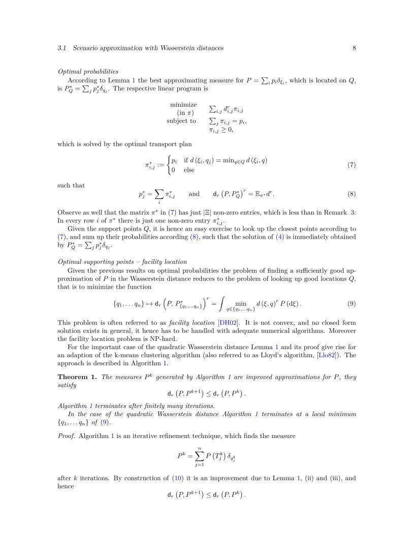
For the important case of the quadratic Wasserstein distance Lemma 1 and its proof give rise foran adaption of the k-means clustering algorithm (also referred to as Lloyd’s algorithm, [Llo82]). Theapproach is described in Algorithm 1.

Theorem 1. The measures P k generated by Algorithm 1 are improved approximations for P , theysatisfy

dr(P, P k+1) ≤ dr

(P, P k

).

Algorithm 1 terminates after finitely many iterations.In the case of the quadratic Wasserstein distance Algorithm 1 terminates at a local minimum

q1, . . . qn of (9).

Proof. Algorithm 1 is an iterative refinement technique, which finds the measure

P k =n∑j=1

P(T kj)δqkj

after k iterations. By construction of (10) it is an improvement due to Lemma 1, (ii) and (iii), andhence

dr(P, P k+1) ≤ dr

(P, P k

).

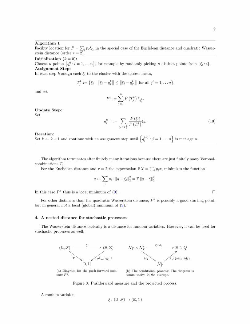
9

Algorithm 1Facility location for P =

∑i piδξi in the special case of the Euclidean distance and quadratic Wasser-

stein distance (order r = 2).Initialization (k = 0):Choose n points

q0i : i = 1, . . . n

, for example by randomly picking n distinct points from ξi : i.

Assignment Step:In each step k assign each ξi to the cluster with the closest mean,

T kj :=ξi :

∥∥ξi − qkj ∥∥ ≤ ∥∥ξi − qkj′∥∥ for all j′ = 1, . . . n

and set

P k :=n∑j=1

P(T kj)δqkj.

Update Step:Set

qk+1j :=

∑ξi∈Tkj

P (ξi)P(T kj)ξi. (10)

Iteration:Set k ← k + 1 and continue with an assignment step until

q

(k)j : j = 1, . . . n

is met again.

The algorithm terminates after finitely many iterations because there are just finitely many Voronoi-combinations Tj .

For the Euclidean distance and r = 2 the expectation EX =∑i pixi minimizes the function

q 7→∑i

pi · ‖q − ξi‖22 = E ‖q − ξ‖22 .

In this case P k thus is a local minimum of (9).

For other distances than the quadratic Wasserstein distance, P k is possibly a good starting point,but in general not a local (global) minimum of (9).

4. A nested distance for stochastic processes

The Wasserstein distance basically is a distance for random variables. However, it can be used forstochastic processes as well:

(Ω,F)

P ##

ξ // (Ξ,Σ)

P ξ=Pξ−1

[0, 1](a) Diagram for the push-forward mea-sure P ξ.

NT ×N ′T

id2 $$

ξid1 // Ξ ⊃ Q

N ′T

Eπ(ξid1 | id2)

<<

(b) The conditional process: The diagram iscommutative in the average.

Figure 3: Pushforward measure and the projected process.

A random variableξ : (Ω,F)→ (Ξ,Σ)

4.1 Definition of the nested distance 10

on a probability space (Ω,F , P ) naturally induce the push-forward measure

P ξ := P ξ−1 : Σ→ [0, 1]

on the state space (Ξ,Σ) (cf. Figure 3a and Figure 1), such that in particular the distance dr(P ξ, P ′ξ

′)

is available by employing a distance function

d : Ξ× Ξ′ → R

defined on the state spaces Ξ × Ξ′. If the spaces Ξ and Ξ′ are interpreted as containing the samplepaths of Stochastic processes, it is possible to consider a process as a random variables, and to applythe Wasserstein distance to the sample paths and their distribution. However, the gradually increasinginformation, which is the essential ingredient of stochastic processes, is simply ignored by just havinga look at the final sigma algebra σ (ξ) ⊂ ΣT instead of the entire filtration (Σ0, . . .ΣT ). Figure 4 showsa situation where similar paths (small ε) lead to a small value of the Wasserstein distance between thefirst and the second case, which neglects the fact that in the second case perfect information aboutthe final outcome is available already at the intermediary step.

These considerations led to the proposal of a nested distance in [Pfl09, PP12].

4.1. Definition of the nested distanceIn the following we will use a multistage (nested) distance concept that shares many properties of

the Wasserstein distances but accounts for the effects of filtrations. It was introduced first in [Pfl09]and analyzed in [PP12]. In order to introduce nested distances we have to generalize the distributionalconcepts used so far from random variables to stochastic processes. For this consider the process(ξt)t∈0,...T, where ξt : (Ω,F) → (Ξt,Σt) are random variables with possibly different state spaces(Ξt, Σt). Define the product space Ξ := Ξ1 × . . .ΞT , which can be equipped itself with the productsigma algebra Σ := σ (Σ1 ⊗ . . .ΣT ). Then

ξ : (Ω,F)→ (Ξ,Σ)ω 7→ (ξt (ω))t∈0,...T

is a random variable, mapping any outcome ω ∈ Ω to its path (ξt (ω))Tt=0. The law of of the process ξ,

P ξ := P ξ−1 : Σ→ [0, 1] ,

is the push-forward measure on Ξ = Ξ1 × . . .ΞT . The situation for processes is completely analogousto random variables, provided that a distance function

d : Ξ× Ξ′ → R

on Ξ = Ξ0 × . . .ΞT and Ξ′ = Ξ′0 × . . .Ξ′T is available. For metric spaces (Ξt, dt) the functionsd (ξ, ξ′) =

∑Tt=0 dt (ξt, ξ′t) or d (ξ, ξ′) = maxt∈0, . . . T dt (ξt, ξ′t) are immediate candidates. We shall

2 2-1

3

p

1

@@@R1 − p

22+ε

1

p

2-εPPPq1 − p

3*1

1HHHj1

2

3

p

1

@@@R

1 − p

3-1

1-1

Figure 4: Three tree processes to illustrate three different flows of information: If ε is small theWasserstein distance will be small too (cf. [HRS06]).

4.2 The nested distance for trees. 11

call a metric (weighted) Euclidean, if d (ξ, ξ′) =(∑T

t=0 wt ‖ξt − ξ′t‖22

)1/2, where wt > 0 are positive

weights and each norm ‖·‖2 satisfies the parallelogram law.With these preparations the nested distances can be defined as follows:

Definition 2. For two filtered probability spaces P := (Ξ,Σ, P ), P′ := (Ξ′,Σ′, P ′) and a real-valued,convex function d : Ξ×Ξ′ → R the nested distance of order r ≥ 1 – denoted dlr (P,Q) – is the optimalvalue of the optimization problem

minimize(in π)

(´d (ξ, ξ′)r π (dξ,dξ′)

) 1r

subject to π (M × Ξ′ | Σt ⊗ Σ′t) = P (M | Σt) (M ∈ ΣT , t ∈ 0, . . . T) ,π (Ξ×N | Σt ⊗ Σ′t) = P ′ (N | Σ′t) (N ∈ Σ′T , t ∈ 0, . . . T) ,

(11)

where the infimum in (11) is among all bivariate probability measures π ∈ P (Ξ× Ξ′), which aremeasures on the product sigma algebra ΣT ⊗ Σ′T . We will refer to the nested distance also as processdistance, or multistage distance. The nested distance dl2 (order r = 2), with d a weighted Euclideandistance is referred to as quadratic nested distance.

Note that the minimization (2) for the Wasserstein distance dr (P, P ′) is a relaxation of (11). Hencethe Wasserstein distance is always less or equal to the nested distance,

dr (P, P ′) ≤ dlr (P,P′) .

It is possible therefore to decompose the nested distance into the Wasserstein and the effect dlr (P,P′)−dr (P, P ′) caused by the filtration related to the additional constraints in (11).

The multistage distance dlr (·, ·) also preserves important regularity properties (Lipschitz and Höldercontinuity) of the objective function of multistage stochastic programs (see [PP12, Section 6]).

4.2. The nested distance for trees.The Wasserstein distance between discrete probability measures can be calculated by solving the

linear program (3). To establish a similar linear program for the nested distance we use trees thatmodel the whole filtration. Then problem (11) reads

minimize(in π)

∑i,j πi,j · dri,j

subject to∑j⊂n π (i, j|m,n) = P (i|m) (m ⊃ i, n),∑i⊂m π (i, j|m,n) = P ′ (j|n) (n ⊃ j, m),

πi,j ≥ 0 and∑i,j πi,j = 1,

(12)

where again πi,j is a matrix defined on the samples (i ∈ NT , j ∈ N ′T ) and m ∈ Nt, n ∈ N ′t arearbitrary nodes. The conditional probabilities π (i, j|m,n) are given by

π (i, j|m,n) = πi,j∑i′⊂m, j′⊂n πi′,j′

.

The nested structure of the transportation plan π, which is induced by the trees, is schematicallydepicted in Figure 5.

The constraints in (12) can be written in more detail

P (i) ·∑

i′⊂m, j′⊂nπi′,j′ = P (m) ·

∑j′⊂n

πi,j′ (m ⊃ i, n) and

P ′ (j) ·∑

i′⊂m, j′⊂nπi′,j′ = P ′ (n) ·

∑i′⊂m

πi′,j (m, n ⊃ j) .

4.2 The nested distance for trees. 12

HHj-*

--

*@@RHHj

*HHj

-

...

*HHj@@R

HHj

@@R -

BBBBBBN

AAU

@@R

-

?

AAUAAU

AAU

AAU

@@R

di,jmm−

n

n−

(Ξ,Σ, P )

(Ξ′,Σ′, P ′)

i

j

(a) Structure of the transport matrix π for two trees,each of height T = 3. m and n are nodes, i and jare leaves.

AAUAAU

AAU

AAU

@@R

AAU

@@R

n

n−

(Ξ′,Σ′, P ′)

j

(b) Structure of the constraints in Al-gorithm 2

Figure 5: Schematic structure of the distance matrix d and the transport matrix π, as it is imposedby the structures of the trees and the respective constraints.

As P and P ′ are given, this shows that (12) is equivalent to the linear program

minimize(in π)

∑i,j πi,j · dri,j

subject to P (i) ·∑i′⊂m, j′⊂n πi′,j′ = P (m) ·

∑j′⊂n πi,j′ (m ⊃ i),

P ′ (j) ·∑i′⊂m, j′⊂n πi′,j′ = P ′ (n) ·

∑i′⊂m πi′,j (n ⊃ j),

πi,j ≥ 0 and∑i,j πi,j = 1.

Remark 3. As a matter of fact many constraints in (12) are linearly dependent. For computationalreasons (loss of significance during numerical evaluations, which can impact linear dependencies andthe feasibility) it is advisable to remove linear dependencies. This is partially accomplished by thesimpler program

minimize(in π)

∑i,j πi,j · dri,j

subject to∑j∈(n−)+

π (m, j|m−, n−) = P (m|m−) (m ∈ N\N0) ,∑i∈(m−)+

π (i, n|m−, n−) = P ′ (n|n−) (n ∈ N ′\N ′0) ,πi,j ≥ 0 and

∑i,j πi,j = 1,

(13)

which by [PP12, Lemma 10] is equivalent to (12) and can be reformulated as an LP as well. Furtherconstraints can be removed from (13) by taking into account that

∑i−=m−

P (i)P (m−) = 1. Hence, for

each node m it is possible to drop one constraint out of all∣∣(m−)+

∣∣ related equations.It should be noted that instead of solving (13) the nested distance can be calculated in a recursive

way. First define

dlr (i, j) := d(ξi, ξ

′j

)(14)

13

for i ∈ NT , j ∈ N ′T . Given dlr (i, j) for i ∈ Nt+1 and j ∈ N ′t+1 set

dlr (m,n)r :=∑

i∈m+,j∈n+

π (i, j|m,n) · dlr (i, j)r (m ∈ Nt, n ∈ N ′t ) (15)

for m ∈ Nt , n ∈ N ′t , where the conditional probabilities π(·, ·|m,n) solve

minimizein π (., .|m,n)

∑i∈m+,j∈n+ π (i, j|m,n) · dlr (i, j)r

subject to∑j∈n+

π (i, j|m,n) = P (i|m) (i ∈ m+),∑i∈m+

π (i, j|m,n) = P ′ (j|n) (j ∈ n+),π (i, j|m,n) ≥ 0.

The values dlr (i, j) can be interpreted as conditional nested distances for the trees starting in nodesi (j, resp.). Finally the transport plan π on the leaves is recomposed by

π (i, j) = π (i, j| iT−1, jT−1) · π (iT−1, jT−1| iT−2, jT−2) · . . . π (i1, j1| 0, 0)

and the nested distance is given by dlr (P,P′)r = dlr (0, 0).

5. Improving an approximating tree

Lemma 1 and the succeeding remark explain how to approximate a probability measure P by ameasure P ∗Q, which is located just on the points Q = q1 . . . qn: the measure P ∗Q =

∑j P (T = qj) ·δqj

(cf. (7)) was found to be the best choice with respect to the Wasserstein distance, irrespective of theorder r ≥ 1. In this section we address the question of looking up processes, i.e. trees, which are closein nested distance to a given tree.

As in Section 3 we split the problem in two parts:

(i) Find probabilities on a given tree structure, which improve the nested distance to a given tree;(ii) facility location: Improve the locations, which are the scenarios of the tree, to again improve the

approximation overall.

5.1. Optimal probabilitiesIn a multistage context we have to answer the question which probability measure P ∗Q is best to

approximate P = (Ξ,Σ, P ), provided that the states Q ⊂ Ξ′ and filtration Σ′ of the stochastic processesare given: Knowing the branching structure of the tree, we seek for the best probabilities such thatthe multistage distance to P is as small as possible. The best approximation, P ∗Q, satisfies

dlr(P,(Ξ′,Σ′, P ∗Q

))≤ dlr (P, (Ξ′,Σ′, P ′)) (P ′ (Q) = 1) ,

where Q = q1, . . . qn ⊂ Ξ′.Compared to the Wasserstein distances it is considerably more difficult to find those optimal prob-

abilities. From (13) it follows that the corresponding transport plan π∗ necessarily satisfies

minimize(in π∗)

∑i,j π

∗i,j · dri,j

subject to∑j π∗ (m, j|m−, n−) = P (m|m−) ,∑

i π∗ (i, n|m−, n−) =

∑i π∗ (i, n| m−, n−) , m, m ∈ Nt

π∗i,j ≥ 0 and∑i,j π

∗i,j = 1.

(16)

The constraint ∑i

π∗ (i, n|m−, n−) =∑i

π∗ (i, n| m−, n−) (m, m ∈ Nt) (17)

5.1 Optimal probabilities 14

for nodes m and m at the same stage t in (16) ensures that

P ∗Q (n|n−) :=∑i

π∗ (i, n|m−, n−)

is well defined (as it is independent of m), allowing thus to reconstruct a measure P ∗Q by P ∗Q =∑j δqj ·

∑i π∗i,j .

Unfortunately, problem (16) does not allow an immediate solution in general. Moreover the con-straints (17), for∑

i⊂m− π∗i,n∑

i⊂m−,j⊂n− π∗i,j

= π∗ (n|m−, n−) = π∗ (n| m−, n−) =∑i⊂m− π

∗i,n∑

i⊂m−,j⊂n− π∗i,j

,

are not linear any more – in fact they are multilinear in π∗.

Recursive computation of the nested distanceFormulation (16) and the fact that the nested distance can be calculated in a recursive way (see

(14) and (15)) leads to the idea of calculating improved probabilities in a recursive way too:Assume that π is feasible for given quantizers Q. Define

dlr (i, j) := d (ξi, qj) (18)

for i ∈ NT , j ∈ N ′T and, given dlr (i, j) for i ∈ Nt+1 and j ∈ N ′t+1, recursively compute

dlr (m,n)r :=∑

i∈m+,j∈n+

π∗ (i, j|m,n) · dlr (i, j)r (m ∈ Nt) (19)

for m ∈ Nt , n ∈ N ′t , where the conditional probabilities π∗ (·, ·|m,n) solve

minimizein π (., .|m,n)

∑m∈Nt π (m,n) ·

∑i∈m+,j∈n+

π (i, j|m,n) · dlr (i, j)r

subject to∑j∈n+

π (i, j|m,n) = P (i|m) (i ∈ m+),∑i∈m+

π (i, j|m,n) =∑i∈m+

π (i, j| m, n) (j ∈ n+),π (i, j|m,n) ≥ 0.

(20)

Recomposing the transport plan π∗ on the leaves i ∈ NT and j ∈ N ′T by

π∗ (i, j) = π∗ (iT , jT | iT−1, jT−1) · π∗ (iT−1, jT−1| iT−2, jT−2) · . . . π∗ (i1, j1| 0, 0) (21)

leads to improved probabilities:

Theorem 2. Let P ′ be the measure related to the feasible transport probabilities π and P ′∗ be relatedto the probabilities π∗ by

P ′∗ :=∑j

δqj ·∑i

π∗ (i, j) .

Then dlr (P,P′∗) ≤ dlr (P,P′) and the improved distance is given by

dlr (P,P′∗) = dlr (0, 0) .

Proof. Observe that the measures π and π∗ have the iterative decomposition

π (i, j) = π (iT , jT )= π (iT , jT | iT−1, jT−1) · π (iT−1, jT−1| iT−2, jT−2) · . . . π (i1, j1| 0, 0) ,

for all leafs i ∈ NT and i ∈ N ′T (cf. [Dur04, Chapter 4, Theorem 1.6]). The terminal distance (t = T ),given the entire history up to (i, j), is dlT ;r (i, j) := d (i, j), which serves as a starting value for the

5.2 Optimal scenarios – facility location 15

iterative procedure. To improve a given transport plan π the algorithm in (20) fixes the conditionalprobabilities π (m,n) in an iterative step at stage t.

The constraints in (20) ensure, for∑i∈m+

∑j∈n+

π∗ (i, j|m,n) =∑i∈m+

P (i|m) = 1,

that π∗ again is a probability measure for each m ∈ N ′t , and hence, by (21), π∗ is a probability measureon NT × N ′T . Furthermore the constraints ensure that π∗ respects the tree structures of both trees:π∗ is feasible for (7). Finally it holds that∑

i,j

π∗i,jd (i, j)r = dlr (0, 0)r

due to the recursive construction.As the initial π is feasible as well for all equations in (20) it follows from the construction that

dlr (P,P′∗)r = dlr (0, 0)r = Eπ∗dr ≤ Eπdr.

As π was chosen arbitrarily it follows that

dlr (P,P′∗) ≤ dlr (P,P′) ,

which shows that P ′∗ is an improvement.

5.2. Optimal scenarios – facility locationConsider quantizers

Q = q1, . . . qn

where each qj = (qj,0, . . . qj,T ) is a path in the tree. Given a fixed, feasible measure π define

Dπ (q1, . . . qn)r := Eπdr =∑i,j

πi,jd (ξi, qj)r . (22)

The problem of finding optimal quantizers consists in solving the minimization problem

minq1,...qn

Dπ (q1, . . . qn) . (23)

Again it is difficult to solve (23), which can be considered as a facility location problem. However, inan iterative procedure as proposed in the following, a few steps of significant descent in each iterationwill be sufficient to considerably improve the overall approximation.

In many applications the gradient of function (22) is available as an analytic expression, for exampleif d

(ξi, ξ

′j

)=(∑

t dt(ξi, ξ

′j

)p)1/p. In this situation the derivative of Dπ (q1, . . . qn)r is given by

∇ξj,tD (ξ′) = Dπ (ξ′)1−r ·∑i

πi,jd(ξi, ξ

′j

)r−p · dt (ξi,t, ξ′j,t)p−1 · ∇ξ′jdt(ξi,t, ξ

′j,t

)(j ∈ Nt) .

If in addition the metric at stage t is a norm, dt(ξi,t, ξ

′j,t

)=∥∥ξi,t − ξ′j,t∥∥s, then it holds that

∇ξ′j,tdt(ξi,t, ξ

′j,t

)= dt

(ξi,t, ξ

′j,t

)1−s · ∣∣ξi,t − ξ′j,t∣∣s−2 ·(ξi,t − ξ′j,t

)which can be obtained by direct computation.

To compute the minimum in (23) a few steps by the steepest descent method will ensure somesuccessive improvements. Another possible method is the limited memory BFGS (Broyden-Fletcher-Goldfarb-Shanno) method, cf [Noc80].

In the special case of the quadratic nested distance the facility location problem can be accomplishedby explicit evaluations. This is by far the fastest procedure, and summarized in Algorithm 2, Step 3.

5.3 The overall algorithm 16

Theorem 3. For a quadratic nested distance the scenarios

qt (nt) :=∑

mt∈Nt

π (mt, nt)∑mt∈Nt π (mt, nt)

· ξt (mt)

(cf. (24)) are the best possible choice to solve the facility location problem (23).

Proof. The explicit decomposition of the nested distance allows for the re-arrangement

dl2 (P,P′)2 =∑i,j

πi,jd (ξi, qj)2

=∑i,j

πi,j

T∑t=0

wt · ‖ξit − qjt‖22

=T∑t=0

wt ·∑nt∈N ′t

( ∑mt∈Nt

π (mt, nt) ‖ξ (mt)− qt (nt)‖22

).

By the same reasoning as in the proof of Theorem 1 the assertion follows for every nt ∈ Nt byconsidering and minimizing every map

q 7→∑

mt∈Nt

π (mt, nt) · ‖ξ (mt)− q‖22

separately.

5.3. The overall algorithmAs it is not possible to improve the probabilities and solve the facility location problem in one single

step Algorithm 2 describes the course of action. Starting with an initial guess for the quantizers (resp.the scenario paths) and using the related transport probabilities π0 the algorithm iterates betweenimproving the quantizers (Step 2) and improving the transport probabilities (Step 3). Step 2 goesbackward in time and uses conditional versions dlk+1

r (m,n) of the nested distance, which are relatedto nodes m and n, in order to resemble an approximation of the full nested distance. To improve thelocations q, Step 3 either uses classical optimization algorithms for the general case, or a version ofthe k-means algorithm in the important case of the quadratic nested distance.

The algorithm leads to an improvement in each iteration step (Theorem 2 and Theorem 3) andconverges in finitely many steps.

Theorem 4. Provided that the minimization (23) can be done exactly – as is the case for the quadraticnested distance – Algorithm 2 terminates at a stationary dlr

(P, P k

∗) after finitely many iterations k∗.

Proof. It is possible – although very inadvisable for computational purposes – to rewrite the compu-tation of dlk+1

r (0, 0) in Algorithm 2 as a single linear program of the form

minimizein πk+1 c

(πk+1|πk

)subject to Aπk+1 = b,

πk+1 ≥ 0,

where the matrix A and the vector b collect all linear conditions from (20), and π 7→ c (π| π) ismultilinear. Note that the constraints Π := π : Aπ = b, π ≥ 0 form a convex polytope, which isindependent of the iterate πk . Without loss of generality one may assume that πk is an edge of thepolytope Π. Because Π has finitely many edges and each edge π ∈ Π can be associated with a uniquequantization scenario q (π), by assumption it is clear that the decreasing sequence

dlk+2r

(P,Pk+2) = c

(πk+2|πk+1) ≤ c (πk+1|πk

)= dlk+1

r

(P,Pk+1)

cannot improve further whenever the stationary point is met.

5.4 A numerical example and derived applications 17

Algorithm 2Sequential improvement of the measure P k to approximate P =

∑i piδξi in the nested distance on the

trees (Ft)t∈0,...T ((F ′t)t∈0,...T, resp.).Step 1– InitializationSet k ← 0, and let q0 be process quantizers with related transport probabilities π0 (i, j) betweenscenario i of the original P-tree and scenario q0

j of the approximating P′-tree; P0 := P′.

Step 2 – Improve the quantizersFind improved quantizers qk+1

j :

• In case of the quadratic Wasserstein distance (Euclidean distance and Wasserstein of order r = 2)set

qk+1 (nt) :=∑

mt∈Nt

πk (mt, nt)∑mt∈Nt π

k (mt, nt)· ξt (mt) , (24)

• or solve (23), for example by applying the steepest descent method, or the limited memory BFGSmethod.

Step 3 – Improve the probabilitiesSetting π ← πk and q ← qk+1 use (18), (19), (20) and (21) to calculate all conditional probabilitiesπk+1 (·, ·|m,n) = π∗ (·, ·|m,n), the unconditional transport probabilities πk+1 (·, ·) and the distancedlk+1r (0, 0) = dlr (0, 0).

Step 4Set k ← k + 1 and continue with Step 2 if

dlk+1r (0, 0) < dlkr (0, 0)− ε,

where ε > 0 is the desired improvement in each cycle k.Otherwise, set q∗ ← qk, define the measure

P k+1 :=∑j

δqk+1j·∑i

πk+1 (i, j) ,

for which dlr(P,Pk+1) = dlk+1

r (0, 0) and stop.Remark. In case of the quadratic nested distance (r = 2) and the Euclidean distance the choice ε = 0is possible.

The same statement as for the Wasserstein distance holds true here for the nested distance: Forother distances than the quadratic ones P k can be used as a starting point, but in general is not evena local minimum.

5.4. A numerical example and derived applications

To illustrate the results we have implemented all steps of the discussed algorithms in MATLAB R©.All LPs were solved using the function linprog. It is a central observation that optimization for Eu-clidean norms and the quadratic Wasserstein distance is fastest. This is because the facility locationproblem can be avoided and replaced by computing the conditional expectation in a direct way. More-over, when applying the methods, it was a repeated pattern that the first few iteration steps improvethe distance significantly, whereas following steps just give minor improvements of the objective.

The computation times collected in Table 1 have been noted for an iteration step in Algorithm 2on a customary, standard laptop.

18

Stages 4 5 5 6 * 7 7Nodes of the initial tree 53 309 188 1,365 1,093 2,426Nodes of the approximating tree 15 15 31 63 127 127Time/ sec. 1 10 4 160 157 1,044

Table 1: Time to perform an iteration in Algorithm 2.The example indicated by the asterisk (*) corresponds to Figure 6.

Figure 6: The initial tree with 1093 nodes at 7 stages (left) and a binary, approximating tree, whichhas 127 nodes (right). Their nested distance is 2.32. The tree structure is depicted, annotated is thehistogram of the paths.

Figure 6 exemplary depicts the situation of the latter example with 7 stages. The computeddistance of 2.32 allows the rough interpretation, that the scenarios of the initial tree – on average –can be squeezed into a “pipe” of radius 2.32/ 7= 0.3 along a branch of the approximating tree.

6. Summary and outlook

In this paper we address the problem of approximating stochastic processes in discrete time bytrees, which are discrete stochastic processes. For this purpose we build on the recently introducednested distances, generalizations of the well known Wasserstein or Kantorovich distances. In additionto their properties as classical probability metrics they are able to account for the effects of filtrationsrelated to stochastic processes.

In particular we use the nested distance to compare trees, which are important tools for discretizingstochastic optimization problems. The aim is to reduce the distance between a given – usually large– tree, and a smaller tree supposed to approximate the given tree. This problem is of fundamentalinterest in stochastic programming, as the number of variables of the initial process can be reducedsignificantly by the techniques and algorithms proposed.

The paper analyzes the relations between processes and trees, reviews the main properties ofWasserstein distances and nested distances and finally proposes and analyzes an iterative algorithmfor improving the nested distance between trees. For the important special case of nested distances oforder 2 based on Euclidean distances the algorithm can be enhanced by using k-means clustering inorder to improve calculation speed.

While first numerical experiences are encouraging, some interesting issues have to be approached infuture research: As an example the speed of the algorithm could be further increased by parallelization,as in its Step 3 many conditional distances can be calculated independently and in parallel for each

19

stage. Furthermore, we will aim at extending the algorithm to improve distances directly betweenstochastic processes and an approximating tree.

7. Acknowledgment

We wish to express our gratitude to Prof. Georg Ch. Pflug for his continual advice. We thank thereferees for their constructive criticism.

8. Bibliography

[Boy71] Edward S. Boylan. Epiconvergence of martingales. Ann. Math. Statist., 42:552–559, 1971.2

[BPP05] V. Bally, G. Pagès, and J. Printems. A quantization tree method for pricing and hedgingmultidimensional american options. Mathematical Finance, 15(1):119–168, 2005. 7

[DGKR03] Jitka Dupačová, Nicole Gröwe-Kuska, and Werner Römisch. Scenario reduction in stochas-tic programming. Mathematical Programming, Ser. A, 95(3):493–511, 2003. 2, 6, 7

[DH02] Z. Drezner and H. W. Hamacher. Facility Location: Applications and Theory. Springer,New York, NY, 2002. 8

[Dur04] Richard A. Durrett. Probability. Theory and Examples. Duxbury Press, Belmont, CA,second edition, 2004. 14

[GL00] Siegfried Graf and Harald Luschgy. Foundations of Quantization for Probability Distribu-tions, volume 1730 of Lecture Notes in Mathematics. Springer-Verlag Berlin Heidelberg,2000. 7

[GS02] A. L. Gibbs and F. E. Su. On choosing and bounding probability metrics. InternationalStatistical Review, 70(3):419–435, 2002. 6

[HR09] Holger Heitsch and Werner Römisch. Scenario tree modeling for multistage stochasticprograms. Math. Program. Ser. A, 118:371–406, 2009. 2

[HRS06] Holger Heitsch, Werner Römisch, and Cyrille Strugarek. Stability of multistage stochasticprograms. SIAM J. Optimization, 17(2):511–525, 2006. 10

[HW01] Kjetil Høyland and Stein W. Wallace. Generating scenario trees for multistage decisionproblems. Management Science, 47:295–307, 2001. 2

[Kla02] Pieter Klaassen. Comment on "generating scenario trees for multistage decision problems".Management Science, 45(11):1512–1516, Nov. 2002. 2

[Kud74] Hirokichi Kudo. A note on the strong convergence of σ-algebras. Ann. Probability, 2:76–83,1974. 2

[Llo82] Stuart P. Lloyd. Least square quantization in PCM. IEEE Transactions of InformationTheory, 28(2):129–137, 1982. 8

[Mon81] Gaspard Monge. Mémoire sue la théorie des déblais et de remblais. Histoire de l’AcadémieRoyale des Sciences de Paris, avec les Mémoires de Mathématique et de Physique pour lamême année, pages 666–704, 1781. 6

[Noc80] Jorge Nocedal. Updating quasi-Newton matrices with limited storage. Mathematics ofComputation, 35(151):773–782, 1980. 15

20

[Pfl09] Georg Ch. Pflug. Version-independence and nested distribution in multistage stochasticoptimization. SIAM Journal on Optimization, 20:1406–1420, 2009. 1, 2, 10

[PP12] Georg Ch. Pflug and Alois Pichler. A distance for multistage stochastic optimizationmodels. SIAM Journal on Optimization, 22(1):1–23, 2012. 10, 11, 12

[PR07] Georg Ch. Pflug and Werner Römisch. Modeling, Measuring and Managing Risk. WorldScientific, River Edge, NJ, 2007. 3

[Rac91] Svetlozar T. Rachev. Probability metrics and the stability of stochastic models. John Wileyand Sons Ltd., West Sussex PO19, 1UD, England, 1991. 6

[SDR09] Alexander Shapiro, Darinka Dentcheva, and Andrzej Ruszczyński. Lectures on StochasticProgramming. MPS-SIAM Series on Optimization 9, 2009. 1

[Shi96] Albert Nikolayevich Shiryaev. Probability. Springer, New York, 1996. 5

[Ver06] Anatoly M. Vershik. Kantorovich metric: Initial history and little-known applications.Journal of Mathematical Sciences, 133(4):1410–1417, 2006. 6

[Vil03] Cédric Villani. Topics in Optimal Transportation, volume 58 of Graduate Studies in Math-ematics. American Mathematical Society, 2003. 6