Scan Conversion

Scan Conversion

• Also known as rasterization• In our programs objects are represented

symbolically– 3D coordinates representing an object’s position– Attributes representing color, motion, etc.

• But, the display device is a 2D array of pixels (unless you’re doing holographic displays)

• Scan Conversion is the process in which an object’s 2D symbolic representation is converted to pixels

• Consider a straight line in 2D– Our program will [most likely] represent it as

two end points of a line segment which is not compatible with what the display expects

– We need a way to perform the conversion

Scan Conversion

(X0, Y0)

(X1, Y1)

Program Space

(X0, Y0)

(X1, Y1)

(Xn, Yn)

Display Space

Drawing Lines

• Equations of a line– Point-Slope Form: y = mx + b (also Ax + By + C = 0)

∆y∆x

m =∆y

∆x

b

Y

X

• As it turns out, this is not very convenient for scan converting a line

Drawing Lines

• Equations of a line– Two Point Form:

– Directly related to the point-slope form but now it allows us to represent a line by two points – which is what most graphics systems use

yxxxxyy

y00

01

01

Drawing Lines

• Equations of a line– Parametric Form:

– By varying t from 0 to 1we can compute all of the points between the end points of the line segment – which is really what we want

tyyyy

txxxx

010

010

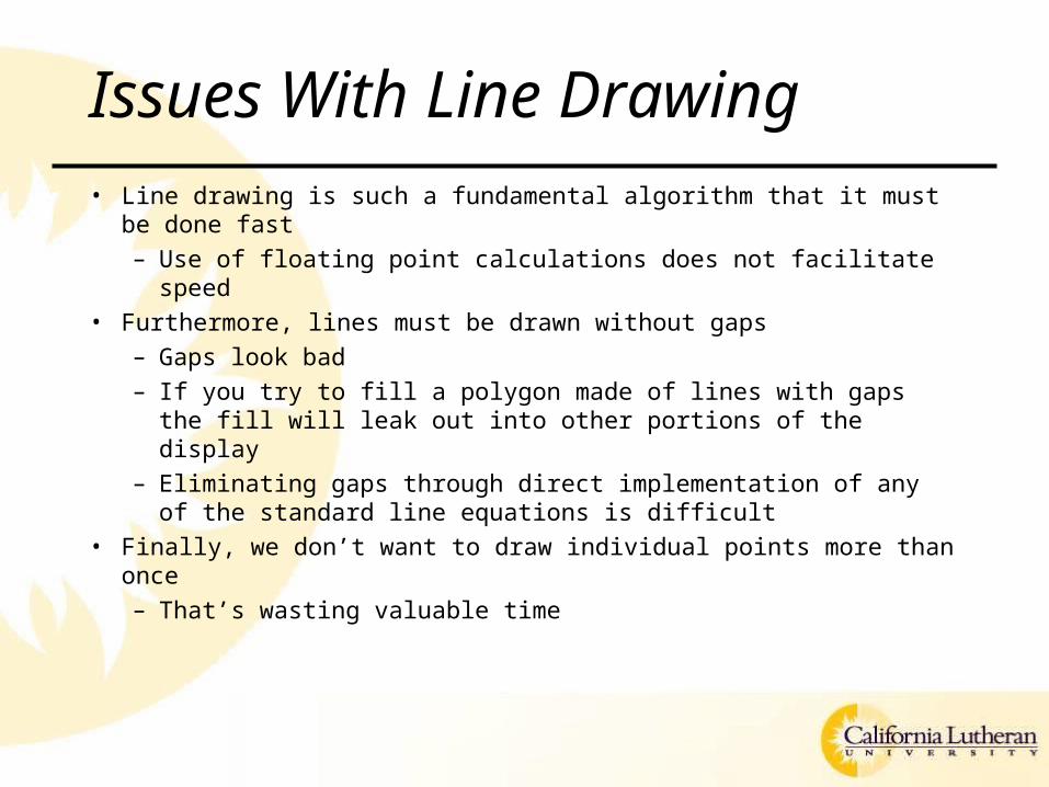
Issues With Line Drawing• Line drawing is such a fundamental algorithm that it must be

done fast– Use of floating point calculations does not facilitate speed

• Furthermore, lines must be drawn without gaps– Gaps look bad– If you try to fill a polygon made of lines with gaps the fill will

leak out into other portions of the display– Eliminating gaps through direct implementation of any of the

standard line equations is difficult• Finally, we don’t want to draw individual points more than once

– That’s wasting valuable time

Bresenham’s Line Drawing Algorithm• Jack Bresenham addressed these issues with the

Bresenham Line Scan Convert algorithm – This was back in 1965 in the days of pen-plotters

• All simple integer calculations– Addition, subtraction, multiplication by 2 (shifts)

• Guarantees connected (gap-less) lines where each point is drawn exactly 1 time

• Also known as the midpoint line algorithm

Bresenham’s Line Algorithm• Consider the two point-slope forms:

algebraic manipulation yields:

where:

yielding:

0, CByAxyxF

bxx

yy

0 bxyxxy

)();(0101 xxyy xy

xByA ;

Bresenham’s Line Algorithm• Assume that the slope of the line segment is

0 ≤ m ≤ 1 • Also, we know that our selection of points is restricted to the grid

of display pixels• The problem is now reduced to a decision of which grid point to

draw at each step along the line– We have to determine how to make our steps

Which point should we choose next?

Bresenham’s Line Algorithm• What it comes down to is computing how close the

midpoint (between the two grid points) is to the actual line

(xp, yp) (xp+1, yp+½)

Bresenham’s Line Algorithm• Define F(m) = d as the discriminant

– (derive from the equation of a line Ax + By + C)

• if (dm > 0) choose the upper point, otherwise choose the lower point

CBAmF

FmF

yxd

yxd

ppm

ppm

)2

1()1()(

)2

1,1(

Bresenham’s Line Algorithm• But this is yet another relatively

complicated computation for every point

• Bresenham’s “trick” is to compute the discriminant incrementally rather than from scratch for every point

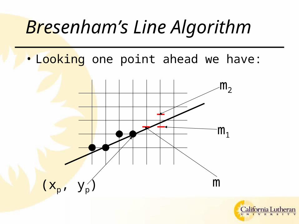
Bresenham’s Line Algorithm• Looking one point ahead we have:

(xp, yp) m

m2

m1

Bresenham’s Line Algorithm• If d > 0 then discriminant is:

• If d < 0 then the next discriminant is:

• These can now be computed incrementally given the proper starting value

CBAF yxdyx ppmpp )

2

3()2()

2

3,2(

2

CBAF yxdyx ppmpp )

2

1()2()

2

1,2(

1

Bresenham’s Line Algorithm• Initial point is (x0, y0) and we know that it is on the line

so F(x0, y0) = 0!• Initial midpoint is (x0+1, y0+½) • Initial discriminant is

F (x0+1, y0+½) = A(x0+1) + B(y0+½) + C

= Ax0+By0+ C + A + B/2

= F(x0, y0) + A + B/2• And we know that F(x0, y0) = 0 so

22

xy

BAd initial

Bresenham’s Line Algorithm• Finally, to do this incrementally we need

to know the differences between the current discriminant (dm) and the two possible next discriminants (dm1 and dm2)

Bresenham’s Line Algorithm

CBAF yxyxd ppppm )

2

1()2()

2

1,2(

1

CBAF yxyxd ppppm )

2

3()2()

2

3,2(

2

CBAF yxyxd ppppcurrent )

2

1()1()

2

1,1(

EyA yydd currentm )(

011

NExyBA xxyydd currentm )()(

01012

We know:

We need (if we choose m1):

or (if we choose m2):

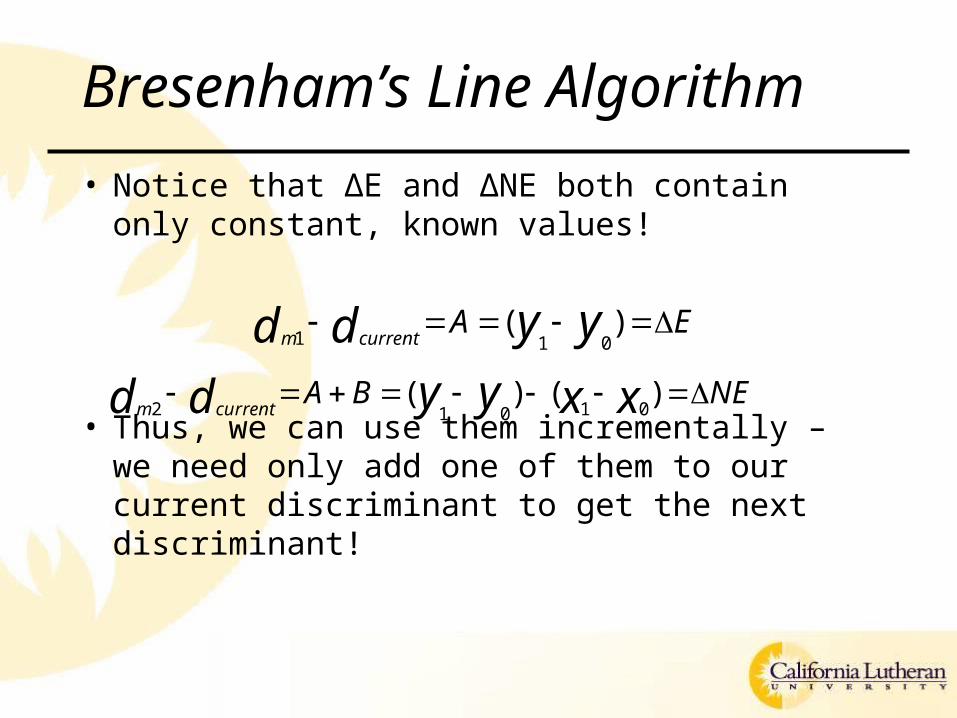
Bresenham’s Line Algorithm• Notice that ΔE and ΔNE both contain only

constant, known values!

• Thus, we can use them incrementally – we need only add one of them to our current discriminant to get the next discriminant!

EA yydd currentm )(

011

NEBA xxyydd currentm )()(

01012

Bresenham’s Line Algorithm• The algorithm then loops through x values in the range of x0

≤ x ≤ x1 computing a y for each x – then plotting the point (x, y)

• Update step– If the discriminant is less than/equal to 0 then increment x, leaving y

alone, and increment the discriminant by ΔE– If the discriminant is greater than 0 then increment x, increment y,

and increment the discriminant by ΔNE• This is for slopes less than 1• If the slope is greater than 1 then loop on y and reverse the

increments of x’s and y’s• Sometimes you’ll see implementations that the discriminant,

ΔE, and ΔNE by 2 (to get rid of the initial divide by 2)• And that is Bresenham’s algorithm

Summary

• Why did we go through all this?• Because it’s an extremely important algorithm• Because the problem demonstrates the

“need for speed” in computer graphics• Because it relates mathematics to computer

graphics (and the math is simple algebraic manipulations)

• Because it presents a nice programming assignment…

Assignment

• Implement Bresenham's approach– You can search the web for this code – it’s out

there– But, be careful because much of the code only

does the slope < 1 case so you’ll have to add the additional code – it’s a copy/paste/edit job

• In your previous assignment, replace your calls to g2d.drawLine with calls to this new method