Embed Size (px)
Citation preview

Scaled Least Squares Estimator for GLMsin Large-Scale Problems
Murat A. ErdogduDepartment of Statistics
Stanford [email protected]
Mohsen BayatiGraduate School of Business
Stanford [email protected]
Lee H. DickerDepartment of Statistics and Biostatistics
Rutgers University and Amazon ⇤
Abstract
We study the problem of efficiently estimating the coefficients of generalized linearmodels (GLMs) in the large-scale setting where the number of observations n ismuch larger than the number of predictors p, i.e. n � p � 1. We show that inGLMs with random (not necessarily Gaussian) design, the GLM coefficients areapproximately proportional to the corresponding ordinary least squares (OLS) coef-ficients. Using this relation, we design an algorithm that achieves the same accuracyas the maximum likelihood estimator (MLE) through iterations that attain up to acubic convergence rate, and that are cheaper than any batch optimization algorithmby at least a factor of O(p). We provide theoretical guarantees for our algorithm,and analyze the convergence behavior in terms of data dimensions. Finally, wedemonstrate the performance of our algorithm through extensive numerical studieson large-scale real and synthetic datasets, and show that it achieves the highestperformance compared to several other widely used optimization algorithms.
1 IntroductionWe consider the problem of efficiently estimating the coefficients of generalized linear models (GLMs)when the number of observations n is much larger than the dimension of the coefficient vector p,(n � p � 1). GLMs play a crucial role in numerous machine learning and statistics problems, andprovide a miscellaneous framework for many regression and classification tasks. Celebrated examplesinclude ordinary least squares, logistic regression, multinomial regression and many applicationsinvolving graphical models [MN89, WJ08, KF09].
The standard approach to estimating the regression coefficients in a GLM is the maximum likelihoodmethod. Under standard assumptions on the link function, the maximum likelihood estimator (MLE)can be written as the solution to a convex minimization problem [MN89]. Due to the non-linearstructure of the MLE problem, the resulting optimization task requires iterative methods. The mostcommonly used optimization technique for computing the MLE is the Newton-Raphson method,which may be viewed as a reweighted least squares algorithm [MN89]. This method uses a secondorder approximation to benefit from the curvature of the log-likelihood and achieves locally quadraticconvergence. A drawback of this approach is its excessive per-iteration cost of O(np
2). To remedy
this, Hessian-free Krylov sub-space based methods such as conjugate gradient and minimal residualare used, but the resulting direction is imprecise [HS52, PS75, Mar10]. On the other hand, first order
⇤Work conducted while at Rutgers University
30th Conference on Neural Information Processing Systems (NIPS 2016), Barcelona, Spain.
approximation yields the gradient descent algorithm, which attains a linear convergence rate withO(np) per-iteration cost. Although its convergence rate is slow compared to that of second ordermethods, its modest per-iteration cost makes it practical for large-scale problems. In the regimen � p, another popular optimization technique is the class of Quasi-Newton methods [Bis95, Nes04],which can attain a per-iteration cost of O(np), and the convergence rate is locally super-linear; awell-known member of this class of methods is the BFGS algorithm [Nes04]. There are recent studiesthat exploit the special structure of GLMs [Erd15], and achieve near-quadratic convergence with aper-iteration cost of O (np), and an additional cost of covariance estimation.
In this paper, we take an alternative approach to fitting GLMs, based on an identity that is well-knownin some areas of statistics, but appears to have received relatively little attention for its computationalimplications in large scale problems. Let �glm denote the GLM regression coefficients, and let �ols
denote the corresponding ordinary least squares (OLS) coefficients (this notation will be definedmore precisely in Section 2). Then, under certain random predictor (design) models,
�
glm / �
ols
. (1)
For logistic regression with Gaussian design (which is equivalent to Fisher’s discriminant analysis),(1) was noted by Fisher in the 1930s [Fis36]; a more general formulation for models with Gaussiandesign is given in [Bri82]. The relationship (1) suggests that if the constant of proportionality isknown, then �
glm can be estimated by computing the OLS estimator, which may be substantiallysimpler than finding the MLE for the original GLM. Our work in this paper builds on this idea.
Our contributions can be summarized as follows.
1. We show that �glm is approximately proportional to �
ols in random design GLMs, regardlessof the predictor distribution. That is, we prove
�
�
�
glm � c ⇥ �
ols
�
�
1 . 1
p
, for some c 2 R.
2. We design a computationally efficient estimator for �glm by first estimating the OLS co-efficients, and then estimating the proportionality constant c . We refer to the resultingestimator as the Scaled Least Squares (SLS) estimator and denote it by ˆ
�
sls. After estimatingthe OLS coefficients, the second step of our algorithm involves finding a root of a real valuedfunction; this can be accomplished using iterative methods with up to a cubic convergencerate and only O(n) per-iteration cost. This is cheaper than the classical batch methodsmentioned above by at least a factor of O(p).
3. For random design GLMs with sub-Gaussian predictors, we show that�
�
�
ˆ
�
sls � �
glm
�
�
�
1. 1
p
+
r
p
n/max {log(n), p} .
This bound characterizes the performance of the proposed estimator in terms of data dimen-sions, and justifies the use of the algorithm in the regime n � p � 1.
4. We study the statistical and computational performance of ˆ
�
sls, and compare it to that of theMLE (using several well-known implementations), on a variety of large-scale datasets.
The rest of the paper is organized as follows: Section 1.1 surveys the related work and Section 2introduces the required background and the notation. In Section 3, we provide the intuition behind therelationship (1), which are based on exact calculations for GLMs with Gaussian design. In Section 4,we propose our algorithm and discuss its computational properties. Section 5 provides a thoroughcomparison between the proposed algorithm and other existing methods. Theoretical results may befound in Section 6. Finally, we conclude with a brief discussion in Section 7.
1.1 Related workAs mentioned in Section 1, the relationship (1) is well-known in several forms in statistics. Brillinger[Bri82] derived (1) for models with Gaussian predictors. Li & Duan [LD89] studied model misspeci-fication problems in statistics and derived (1) when the predictor distribution has linear conditionalmeans (this is a slight generalization of Gaussian predictors). More recently, Stein’s lemma [BEM13]and the relationship (1) has been revisited in the context of compressed sensing [PV15, TAH15],where it has been shown that the standard lasso estimator may be very effective when used in models
2
where the relationship between the expected response and the signal is nonlinear, and the predictors(i.e. the design or sensing matrix) are Gaussian. A common theme for all of this previous work is thatit focuses solely on settings where (1) holds exactly and the predictors are Gaussian (or, in [LD89],nearly Gaussian). Two key novelties of the present paper are (i) our focus on the computationalbenefits following from (1) for large scale problems with n � p � 1; and (ii) our rigorous analysisof models with non-Gaussian predictors, where (1) is shown to be approximately valid.
2 Preliminaries and notationWe assume a random design setting, where the observed data consists of n random iid pairs (y1, x1),(y2, x2), . . ., (yn, xn); yi 2 R is the response variable and xi = (xi1, . . . , xip)
T 2 Rp is the vectorof predictors or covariates. We focus on problems where fitting a GLM is desirable, but we do notneed to assume that (yi, xi) are actually drawn from the corresponding statistical model (i.e. weallow for model misspecification).
The MLE for GLMs with canonical link is defined by
ˆ
�
mle
= argmax
�2Rp
1
n
nX
i=1
yihxi,�i � (hxi,�i). (2)
where h·, ·i denotes the Euclidean inner-product on Rp, and is a sufficiently smooth convex function.The GLM coefficients �glm are defined by taking the population average in (2):
�
glm
= argmax
�2RpE [yihxi,�i � (hxi,�i)] . (3)
While we make no assumptions on beyond smoothness, note that if is the cumulant generatingfunction for yi | xi, then we recover the standard GLM with canonical link and regression parameters�
glm [MN89]. Examples of GLMs in this form include logistic regression, with (w) = log{1+e
w};Poisson regression, with (w) = e
w; and linear regression (least squares), with (w) = w
2/2.
Our objective is to find a computationally efficient estimator for �
glm. The alternative estima-tor for �glm proposed in this paper is related to the OLS coefficient vector, which is defined by�
ols
:
= E[xixTi ]
�1E [xiyi]; the corresponding OLS estimator is ˆ
�
ols
:
= (XTX)
�1XTy, where
X = (x1, . . . , xn)T is the n⇥ p design matrix and y = (y1, . . . , yn)
T 2 Rn.
Additionally, throughout the text we let [m]={1, 2, ...,m}, for positive integers m, and we denotethe size of a set S by |S|. The m-th derivative of a function g : R ! R is denoted by g
(m). Fora vector u 2 Rp and a n ⇥ p matrix U, we let kukq and kUkq denote the `q-vector and -operatornorms, respectively. If S ✓ [n], let US denote the |S|⇥ p matrix obtained from U by extracting therows that are indexed by S. For a symmetric matrix M 2 Rp⇥p, �max(M) and �min(M) denote themaximum and minimum eigenvalues, respectively. ⇢k(M) denotes the condition number of M withrespect to k-norm. We denote by Nq the q-variate normal distribution.
3 OLS is equivalent to GLM up to a scalar factorTo motivate our methodology, we assume in this section that the covariates are multivariate normal,as in [Bri82]. These distributional assumptions will be relaxed in Section 6.Proposition 1. Assume that the covariates are multivariate normal with mean 0 and covariancematrix ⌃ = E
⇥
xixTi
⇤
, i.e. xi ⇠ Np(0,⌃). Then �
glm can be written as
�
glm
= c ⇥ �
ols
,
where c 2 R satisfies the equation 1 = c E⇥
(2)(hx,�olsic )
⇤
.
Proof of Proposition 1. The optimal point in the optimization problem (3), has to satisfy the followingnormal equations,
E [yixi] = Eh
xi (1)
(hxi,�i)i
. (4)
Now, denote by �(x | ⌃) the multivariate normal density with mean 0 and covariance matrix ⌃. Werecall the well-known property of Gaussian density d�(x | ⌃)/dx = �⌃�1
x�(x | ⌃). Using this
3
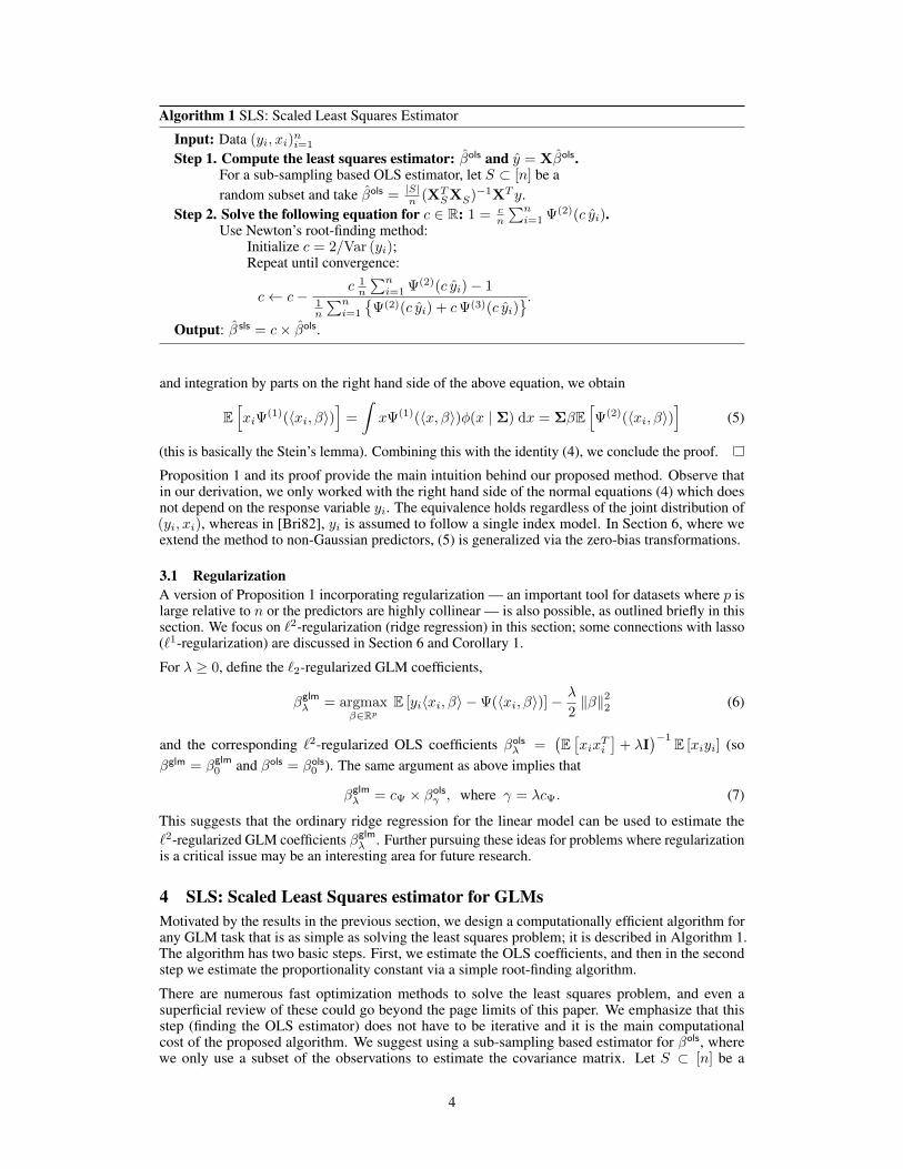
Algorithm 1 SLS: Scaled Least Squares Estimator
Input: Data (yi, xi)ni=1
Step 1. Compute the least squares estimator: ˆ
�
ols and y = Xˆ
�
ols.For a sub-sampling based OLS estimator, let S ⇢ [n] be arandom subset and take ˆ
�
ols
=
|S|n (XT
SXS)�1XT
y.Step 2. Solve the following equation for c 2 R: 1 =
cn
Pni=1
(2)(c yi).
Use Newton’s root-finding method:Initialize c = 2/Var (yi);Repeat until convergence:
c c� c
1n
Pni=1
(2)(c yi)� 1
1n
Pni=1
�
(2)(c yi) + c
(3)(c yi)
.
Output: ˆ
�
sls
= c⇥ ˆ
�
ols.
and integration by parts on the right hand side of the above equation, we obtain
Eh
xi (1)
(hxi,�i)i
=
Z
x
(1)(hx,�i)�(x | ⌃) dx = ⌃�E
h
(2)(hxi,�i)
i
(5)
(this is basically the Stein’s lemma). Combining this with the identity (4), we conclude the proof.
Proposition 1 and its proof provide the main intuition behind our proposed method. Observe thatin our derivation, we only worked with the right hand side of the normal equations (4) which doesnot depend on the response variable yi. The equivalence holds regardless of the joint distribution of(yi, xi), whereas in [Bri82], yi is assumed to follow a single index model. In Section 6, where weextend the method to non-Gaussian predictors, (5) is generalized via the zero-bias transformations.
3.1 RegularizationA version of Proposition 1 incorporating regularization — an important tool for datasets where p islarge relative to n or the predictors are highly collinear — is also possible, as outlined briefly in thissection. We focus on `
2-regularization (ridge regression) in this section; some connections with lasso(`1-regularization) are discussed in Section 6 and Corollary 1.
For � � 0, define the `2-regularized GLM coefficients,
�
glm
� = argmax
�2RpE [yihxi,�i � (hxi,�i)]� �
2
k�k22 (6)
and the corresponding `
2-regularized OLS coefficients �
ols
� =
�
E⇥
xixTi
⇤
+ �I��1 E [xiyi] (so
�
glm
= �
glm
0 and �
ols
= �
ols
0 ). The same argument as above implies that
�
glm
� = c ⇥ �
ols
� , where � = �c . (7)
This suggests that the ordinary ridge regression for the linear model can be used to estimate the`
2-regularized GLM coefficients �glm
� . Further pursuing these ideas for problems where regularizationis a critical issue may be an interesting area for future research.
4 SLS: Scaled Least Squares estimator for GLMsMotivated by the results in the previous section, we design a computationally efficient algorithm forany GLM task that is as simple as solving the least squares problem; it is described in Algorithm 1.The algorithm has two basic steps. First, we estimate the OLS coefficients, and then in the secondstep we estimate the proportionality constant via a simple root-finding algorithm.
There are numerous fast optimization methods to solve the least squares problem, and even asuperficial review of these could go beyond the page limits of this paper. We emphasize that thisstep (finding the OLS estimator) does not have to be iterative and it is the main computationalcost of the proposed algorithm. We suggest using a sub-sampling based estimator for �ols, wherewe only use a subset of the observations to estimate the covariance matrix. Let S ⇢ [n] be a
4
0
20
40
60
4 5 6log10(n)
Tim
e(se
c)
MethodSLSMLE
SLS vs MLE : Computation
0.0
0.3
0.6
0.9
1.2
4 5 6log10(n)
|β−β|
2
MethodSLSMLE
SLS vs MLE : Accuracy
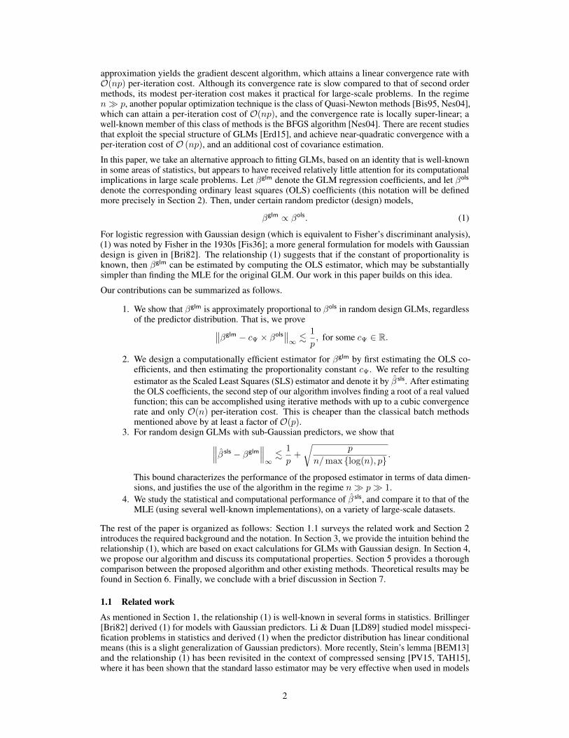
Figure 1: Logistic regression with general Gaussian design. The left plot shows the computational cost (time)for finding the MLE and SLS as n grows and p = 200. The right plot depicts the accuracy of the estimators.In the regime where the MLE is expensive to compute, the SLS is found much more rapidly and has the sameaccuracy. R’s built-in functions are used to find the MLE.
random sub-sample and denote by XS the sub-matrix formed by the rows of X in S. Then thesub-sampled OLS estimator is given as ˆ
�
ols
=
�
1|S|X
TSXS
��1 1nX
Ty. Properties of this estimator
have been well-studied [Ver10, DLFU13, EM15]. For sub-Gaussian covariates, it suffices to usea sub-sample size of O (p log(p)) [Ver10]. Hence, this step requires a single time computationalcost of O �|S|p2 + p
3+ np
� ⇡ O �
pmax{p2 log(p), n}�. For other approaches, we refer reader to[RT08, DLFU13] and the references therein.
The second step of Algorithm 1 involves solving a simple root-finding problem. As with the firststep of the algorithm, there are numerous methods available for completing this task. Newton’sroot-finding method with quadratic convergence or Halley’s method with cubic convergence may beappropriate choices. We highlight that this step costs only O (n) per-iteration and that we can attain upto a cubic rate of convergence. The resulting per-iteration cost is cheaper than other commonly usedbatch algorithms by at least a factor of O (p) — indeed, the cost of computing the gradient is O (np).For simplicity, we use Newton’s root-finding method initialized at c = 2/Var (yi). Assuming thatthe GLM is a good approximation to the true conditional distribution, by the law of total variance andbasic properties of GLMs, we have
Var (yi) = E [Var (yi | xi)] + Var (E [yi | xi]) ⇡ c
�1 + Var
�
(1)(hxi,�i)
�
. (8)
It follows that this initialization is reasonable as long as c�1 ⇡ E [Var (yi | xi)] is not much smaller
than Var�
(1)(hxi,�i)
�
. Our experiments show that SLS is very robust to initialization.
In Figure 1, we compare the performance of our SLS estimator to that of the MLE, when both are usedto analyze synthetic data generated from a logistic regression model under general Gaussian designwith randomly generated covariance matrix. The left plot shows the computational cost of obtainingboth estimators as n increases for fixed p. The right plot shows the accuracy of the estimators. In theregime n � p � 1 — where the MLE is hard to compute — the MLE and the SLS achieve the sameaccuracy, yet SLS has significantly smaller computation time. We refer the reader to Section 6 fortheoretical results characterizing the finite sample behavior of the SLS.
5 ExperimentsThis section contains the results of a variety of numerical studies, which show that the Scaled LeastSquares estimator reaches the minimum achievable test error substantially faster than commonly usedbatch algorithms for finding the MLE. Both logistic and Poisson regression models (two types ofGLMs) are utilized in our analyses, which are based on several synthetic and real datasets.
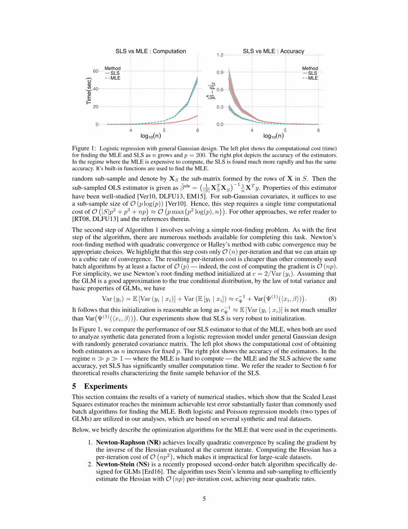
Below, we briefly describe the optimization algorithms for the MLE that were used in the experiments.
1. Newton-Raphson (NR) achieves locally quadratic convergence by scaling the gradient bythe inverse of the Hessian evaluated at the current iterate. Computing the Hessian has aper-iteration cost of O �
np
2�
, which makes it impractical for large-scale datasets.2. Newton-Stein (NS) is a recently proposed second-order batch algorithm specifically de-
signed for GLMs [Erd16]. The algorithm uses Stein’s lemma and sub-sampling to efficientlyestimate the Hessian with O (np) per-iteration cost, achieving near quadratic rates.
5
Rand
omstart
OLSstart
Logis0cRegression PoissonRegression
(a)
(b)
(c) (e) (g)
(d) (f) (h)
0.2
0.3
0.4
0.5
0 10 20 30 40 50Time (sec)
Test
Erro
r
SLSNRNSBFGSLBFGSGDAGD
Log−Reg / Covariates ~ Σ x {Exp(1)−1}
0.22
0.24
0.26
0.28
0.30
0 10 20 30 40 50Time (sec)
Test
Erro
r
SLSNRNSBFGSLBFGSGDAGD
Log−Reg / Higgs dataset
0.23
0.24
0.25
0 10 20 30 40Time (sec)
Test
Erro
r
SLSNRNSBFGSLBFGSGDAGD
Log−Reg / Higgs dataset
0.18
0.20
0.22
0.24
0 5 10 15 20Time (sec)
Test
Erro
r
SLSNRNSBFGSLBFGSGDAGD
Log−Reg / Covariates ~ Σ x {Exp(1)−1}
0.5
1.0
1.5
2.0
0 10 20 30 40Time (sec)
log(
Test
Erro
r)
SLSNRNSBFGSLBFGSGDAGD
Poi−Reg / Covariates ~ Σ x Ber( ± 1)
0.5
1.0
1.5
2.0
2.5
0 10 20 30 40Time (sec)
log(
Test
Erro
r)
SLSNRNSBFGSLBFGSGDAGD
Poi−Reg / Covariates ~ Σ x Ber( ± 1)
0
5
10
15
0.0 2.5 5.0 7.5 10.0Time (sec)
log(
Test
Erro
r)
SLSNRNSBFGSLBFGSGDAGD
Poi−Reg / Covertype dataset
0.5
1.0
1.5
2.0
0.0 2.5 5.0 7.5 10.0Time (sec)
log(
Test
Erro
r)
SLSNRNSBFGSLBFGSGDAGD
Poi−Reg / Covertype dataset
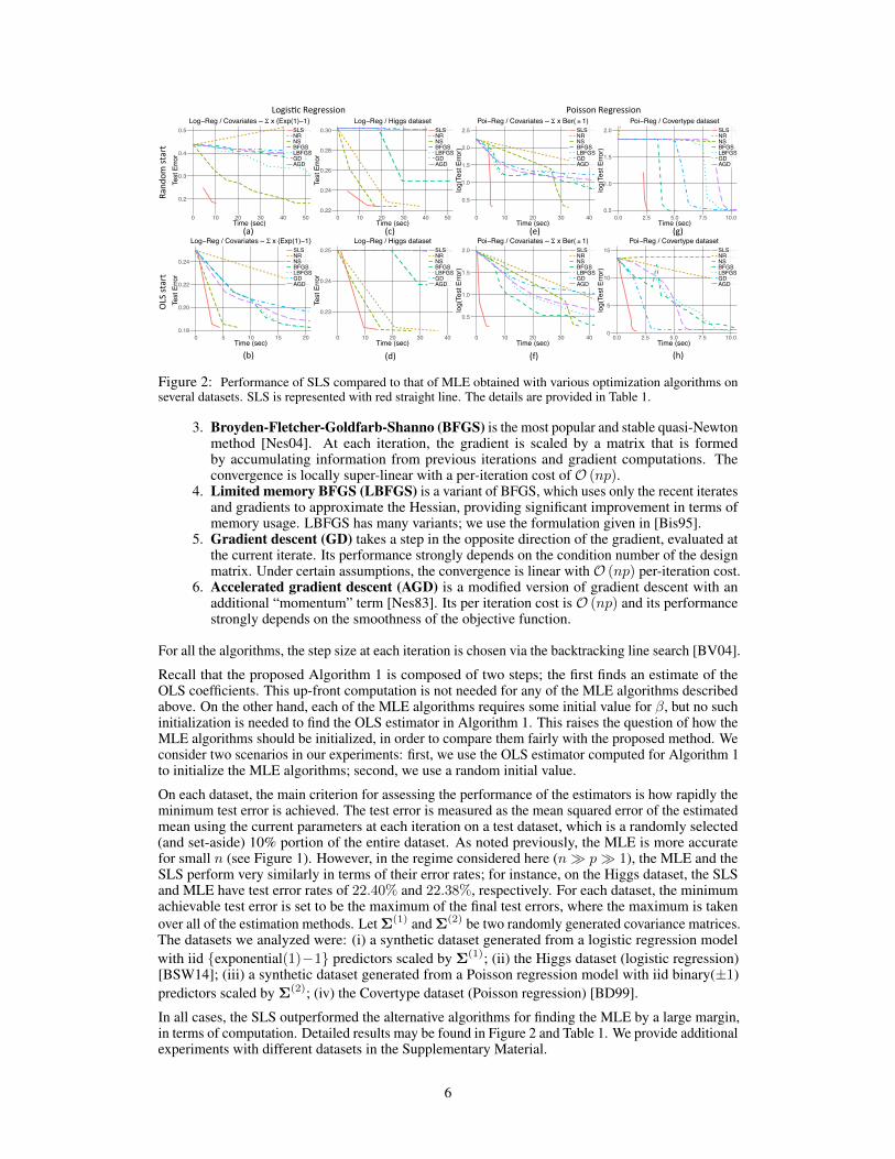
Figure 2: Performance of SLS compared to that of MLE obtained with various optimization algorithms onseveral datasets. SLS is represented with red straight line. The details are provided in Table 1.
3. Broyden-Fletcher-Goldfarb-Shanno (BFGS) is the most popular and stable quasi-Newtonmethod [Nes04]. At each iteration, the gradient is scaled by a matrix that is formedby accumulating information from previous iterations and gradient computations. Theconvergence is locally super-linear with a per-iteration cost of O (np).
4. Limited memory BFGS (LBFGS) is a variant of BFGS, which uses only the recent iteratesand gradients to approximate the Hessian, providing significant improvement in terms ofmemory usage. LBFGS has many variants; we use the formulation given in [Bis95].
5. Gradient descent (GD) takes a step in the opposite direction of the gradient, evaluated atthe current iterate. Its performance strongly depends on the condition number of the designmatrix. Under certain assumptions, the convergence is linear with O (np) per-iteration cost.
6. Accelerated gradient descent (AGD) is a modified version of gradient descent with anadditional “momentum” term [Nes83]. Its per iteration cost is O (np) and its performancestrongly depends on the smoothness of the objective function.
For all the algorithms, the step size at each iteration is chosen via the backtracking line search [BV04].
Recall that the proposed Algorithm 1 is composed of two steps; the first finds an estimate of theOLS coefficients. This up-front computation is not needed for any of the MLE algorithms describedabove. On the other hand, each of the MLE algorithms requires some initial value for �, but no suchinitialization is needed to find the OLS estimator in Algorithm 1. This raises the question of how theMLE algorithms should be initialized, in order to compare them fairly with the proposed method. Weconsider two scenarios in our experiments: first, we use the OLS estimator computed for Algorithm 1to initialize the MLE algorithms; second, we use a random initial value.
On each dataset, the main criterion for assessing the performance of the estimators is how rapidly theminimum test error is achieved. The test error is measured as the mean squared error of the estimatedmean using the current parameters at each iteration on a test dataset, which is a randomly selected(and set-aside) 10% portion of the entire dataset. As noted previously, the MLE is more accuratefor small n (see Figure 1). However, in the regime considered here (n � p � 1), the MLE and theSLS perform very similarly in terms of their error rates; for instance, on the Higgs dataset, the SLSand MLE have test error rates of 22.40% and 22.38%, respectively. For each dataset, the minimumachievable test error is set to be the maximum of the final test errors, where the maximum is takenover all of the estimation methods. Let ⌃(1) and ⌃(2) be two randomly generated covariance matrices.The datasets we analyzed were: (i) a synthetic dataset generated from a logistic regression modelwith iid {exponential(1)�1} predictors scaled by ⌃(1); (ii) the Higgs dataset (logistic regression)[BSW14]; (iii) a synthetic dataset generated from a Poisson regression model with iid binary(±1)predictors scaled by ⌃(2); (iv) the Covertype dataset (Poisson regression) [BD99].
In all cases, the SLS outperformed the alternative algorithms for finding the MLE by a large margin,in terms of computation. Detailed results may be found in Figure 2 and Table 1. We provide additionalexperiments with different datasets in the Supplementary Material.
6
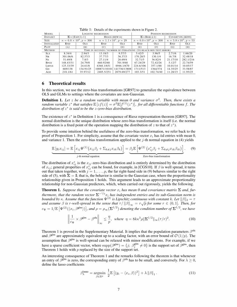
Table 1: Details of the experiments shown in Figure 2.MODEL LOGISTIC REGRESSION POISSON REGRESSIONDATASET ⌃⇥{EXP(1)-1} HIGGS [BSW14] ⌃⇥BER(±1) COVERTYPE [BD99]SIZE n = 6.0 ⇥ 105 , p = 300 n = 1.1⇥107 , p = 29 n = 6.0⇥105 , p = 300 n = 5.8⇥105 , p = 53INITIALIZED RND OLS RND OLS RND OLS RND OLSPLOT (A) (B) (C) (D) (E) (F) (G) (H)METHOD TIME IN SECONDS / NUMBER OF ITERATIONS (TO REACH MIN TEST ERROR)SLS 8.34/4 2.94/3 13.18/3 9.57/3 5.42/5 3.96/5 2.71/6 1.66/20NR 301.06/6 82.57/3 37.77/3 36.37/3 170.28/5 130.1/4 16.7/8 32.48/18NS 51.69/8 7.8/3 27.11/4 26.69/4 32.71/5 36.82/4 21.17/10 282.1/216BFGS 148.43/31 24.79/8 660.92/68 701.9/68 67.24/29 72.42/26 5.12/7 22.74/59LBFGS 125.33/39 24.61/8 6368.1/651 6946.1/670 224.6/106 357.1/88 10.01/14 10.05/17GD 669/138 134.91/25 100871/10101 141736/13808 1711/513 1364/374 14.35/25 33.58/87AGD 218.1/61 35.97/12 2405.5/251 2879.69/277 103.3/51 102.74/40 11.28/15 11.95/25
6 Theoretical resultsIn this section, we use the zero-bias transformations [GR97] to generalize the equivalence betweenOLS and GLMs to settings where the covariates are non-Gaussian.Definition 1. Let z be a random variable with mean 0 and variance �
2. Then, there exists arandom variable z
⇤ that satisfies E [zf(z)] = �
2E[f (1)(z
⇤)], for all differentiable functions f . The
distribution of z⇤ is said to be the z-zero-bias distribution.
The existence of z⇤ in Definition 1 is a consequence of Riesz representation theorem [GR97]. Thenormal distribution is the unique distribution whose zero-bias transformation is itself (i.e. the normaldistribution is a fixed point of the operation mapping the distribution of z to that of z⇤).
To provide some intuition behind the usefulness of the zero-bias transformation, we refer back to theproof of Proposition 1. For simplicity, assume that the covariate vector xi has iid entries with mean 0,and variance 1. Then the zero-bias transformation applied to the j-th normal equation in (4) yields
E [yixij ] = Eh
xij (1)
�
xij�j + ⌃k 6=jxik�k
�
i
| {z }
j-th normal equation
= �jEh
(2)�
x
⇤ij�j + ⌃k 6=jxik�ik
�
i
| {z }
Zero-bias transformation
. (9)
The distribution of x⇤ij is the xij-zero-bias distribution and is entirely determined by the distribution
of xij ; general properties of x⇤ij can be found, for example, in [CGS10]. If � is well spread, it turns
out that taken together, with j = 1, . . . , p, the far right-hand side in (9) behaves similar to the rightside of (5), with ⌃ = I; that is, the behavior is similar to the Gaussian case, where the proportionalityrelationship given in Proposition 1 holds. This argument leads to an approximate proportionalityrelationship for non-Gaussian predictors, which, when carried out rigorously, yields the following.Theorem 1. Suppose that the covariate vector xi has mean 0 and covariance matrix ⌃ and, fur-thermore, that the random vector ⌃�1/2
xi has independent entries and its sub-Gaussian norm isbounded by . Assume that the function (2) is Lipschitz continuous with constant k. Let k�k2 = ⌧
and assume � is r-well-spread in the sense that ⌧/ k�k1 = r
pp for some r 2 (0, 1]. Then, for
c = 1/E⇥
(2)(hxi,�
glmi)⇤, and ⇢ = ⇢1(⌃1/2) denoting the condition number of ⌃1/2, we have
�
�
�
�
1
c ⇥ �
glm � �
ols
�
�
�
�
1 ⌘
p
, where ⌘ = 8k
3⇢k⌃1/2k1(⌧/r)
2. (10)
Theorem 1 is proved in the Supplementary Material. It implies that the population parameters �ols
and �
glm are approximately equivalent up to a scaling factor, with an error bound of O (1/p). Theassumption that �glm is well-spread can be relaxed with minor modifications. For example, if wehave a sparse coefficient vector, where supp(�
glm
) = {j; �glm
j 6= 0} is the support set of �glm, thenTheorem 1 holds with p replaced by the size of the support set.
An interesting consequence of Theorem 1 and the remarks following the theorem is that wheneveran entry of �glm is zero, the corresponding entry of �ols has to be small, and conversely. For � � 0,define the lasso coefficients
�
lasso
� = argmin
�2Rp
1
2
E⇥
(yi � hxi,�i)2⇤
+ � k�k1 . (11)
7
Corollary 1. For any � � ⌘/|supp(�glm
)|, if E [xi] = 0 and E⇥
xixTi
⇤
= I, we havesupp(�
lasso
) ⇢ supp(�
glm
). Further, if � and �
glm also satisfy that 8j 2 supp(�
glm
), |�glm
j | >c
�
�+ ⌘/|supp(�glm
)|�, then we have supp(�
lasso
) = supp(�
glm
).
So far in this section, we have only discussed properties of the population parameters, such as �glm.In the remainder of this section, we turn our attention to results for the estimators that are the mainfocus of this paper; these results ultimately build on our earlier results, i.e. Theorem 1.
In order to precisely describe the performance of ˆ
�
sls, we first need bounds on the OLS estimator.The OLS estimator has been studied extensively in the literature; however, for our purposes, wefind it convenient to derive a new bound on its accuracy. While we have not seen this exact boundelsewhere, it is very similar to Theorem 5 of [DLFU13].Proposition 2. Assume that E [xi] = 0, E
⇥
xixTi
⇤
= ⌃, and that ⌃�1/2xi and yi are sub-Gaussian
with norms and �, respectively. For �min denoting the smallest eigenvalue of ⌃, and |S| > ⌘p,�
�
�
ˆ
�
ols � �
ols
�
�
�
2 ⌘�
�1/2
min
r
p
|S| , (12)
with probability at least 1� 3e
�p, where ⌘ depends only on � and .
Proposition 2 is proved in the Supplementary Material. Our main result on the performance of ˆ
�
sls isgiven next.Theorem 2. Let the assumptions of Theorem 1 and Proposition 2 hold with E[k⌃�1/2
xk2] = µ
pp.
Further assume that the function f(z) = zE⇥
(2)(hx,�olsiz)⇤ satisfies f(c) > 1 +
¯
�
pp for some c
and ¯
� such that the derivative of f in the interval [0, c] does not change sign, i.e., its absolute value islower bounded by � > 0. Then, for n and |S| sufficiently large, we have
�
�
�
ˆ
�
sls � �
glm
�
�
�
1 ⌘1
1
p
+ ⌘2
r
p
min {n/ log(n), |S|/p} , (13)
with probability at least 1� 5e
�p, where the constants ⌘1 and ⌘2 are defined by⌘1 =⌘kc
3⇢k⌃1/2k1(⌧/r)
2 (14)
⌘2 =⌘c�
�1/2min
⇣
1 + �
�1�
1/2min k�olsk1 max {(b+ k/µ), kc}
⌘
, (15)
and ⌘ > 0 is a constant depending on and �.
Note that the convergence rate of the upper bound in (13) depends on the sum of the two terms, bothof which are functions of the data dimensions n and p. The first term on the right in (13) comes fromTheorem 1, which bounds the discrepancy between c ⇥ �
ols and �
glm. This term is small when p islarge, and it does not depend on the number of observations n.
The second term in the upper bound (13) comes from estimating �
ols and c . This term is increasingin p, which reflects the fact that estimating �
glm is more challenging when p is large. As expected,this term is decreasing in n and |S|, i.e. larger sample size yields better estimates. When the full OLSsolution is used (|S| = n), the second term becomes O(
p
pmax{log(n), p}/n) = O(p/
pn), for p
sufficiently large. This suggests that n should be at least of order p2 for good performance.
7 Discussion
In this paper, we showed that the coefficients of GLMs and OLS are approximately proportionalin the general random design setting. Using this relation, we proposed a computationally efficientalgorithm for large-scale problems that achieves the same accuracy as the MLE by first estimating theOLS coefficients and then estimating the proportionality constant through iterations that can attainquadratic or cubic convergence rate, with only O (n) per-iteration cost.
We briefly mentioned that the proportionality between the coefficients holds even when there isregularization in Section 3.1. Further pursuing this idea may be interesting for large-scale problemswhere regularization is crucial. Another interesting line of research is to find similar proportionalityrelations between the parameters in other large-scale optimization problems such as support vectormachines. Such relations may reduce the problem complexity significantly.
8
References[BD99] J. A. Blackard and D. J. Dean, Comparative accuracies of artificial neural networks and discriminant
analysis in predicting forest cover types from cartographic variables, Comput. Electron. Agr. 24(1999), 131–151.
[BEM13] M. Bayati, M. A. Erdogdu, and A. Montanari, Estimating lasso risk and noise level, NIPS 26, 2013,pp. 944–952.
[Bis95] C. M. Bishop, Neural Networks for Pattern Recognition, Oxford University Press, 1995.[Bri82] D. R Brillinger, A generalized linear model with "Gaussian" regressor variables, A Festschrift For
Erich L. Lehmann, CRC Press, 1982, pp. 97–114.[BSW14] P. Baldi, P. Sadowski, and D. Whiteson, Searching for exotic particles in high-energy physics with
deep learning, Nat. Commun. 5 (2014), 4308–4308.[BV04] S. Boyd and L. Vandenberghe, Convex Optimization, Cambridge University Press, 2004.[CGS10] L. H. Y. Chen, L. Goldstein, and Q.-M. Shao, Normal approximation by Stein’s method, Springer,
2010.[DLFU13] P. Dhillon, Y. Lu, D. P. Foster, and L. Ungar, New subsampling algorithms for fast least squares
regression, NIPS 26 (2013), 360–368.[EM15] M. A. Erdogdu and A. Montanari, Convergence rates of sub-sampled newton methods, NIPS 28,
2015, pp. 3034–3042.[Erd15] M. A. Erdogdu, Newton-Stein method: A second order method for GLMs via Stein’s lemma, NIPS
28 (2015), 1216–1224.[Erd16] , Newton-Stein Method: An optimization method for GLMs via Stein’s Lemma, Journal of
Machine Learning Research (to appear) (2016).[Fis36] R. A. Fisher, The use of multiple measurements in taxonomic problems, Ann. Eugenic 7 (1936),
179–188.[Gol07] L. Goldstein, l1 bounds in normal approximation, Ann. Probab. 35 (2007), 1888–1930.[GR97] L. Goldstein and G. Reinert, Stein’s method and the zero bias transformation with application to
simple random sampling, Ann. Appl. Probab. 7 (1997), 935–952.[HS52] M. R. Hestenes and E. Stiefel, Methods of conjugate gradients for solving linear systems, J. Res.
Nat. Bur. Stand. 49 (1952), 409–436.[KF09] D. Koller and N. Friedman, Probabilistic Graphical Models: Principles and Techniques, MIT press,
2009.[LD89] K.-C. Li and N. Duan, Regression analysis under link violation, Ann. Stat. 17 (1989), 1009–1052.[Mar10] J. Martens, Deep learning via Hessian-free optimization, ICML 27 (2010), 735–742.[MN89] P. McCullagh and J. A. Nelder, Generalized Linear Models, 2nd ed., Chapman and Hall, 1989.[Nes83] Y. Nesterov, A method of solving a convex programming problem with convergence rate O(1/k2),
Soviet Math. Dokl. 27 (1983), 372–376.[Nes04] , Introductory Lectures on Convex Optimization: A Basic Course, Springer, 2004.[PS75] C. C. Paige and M. A. Saunders, Solution of sparse indefinite systems of linear equations, SIAM J.
Numer. Anal. 12 (1975), 617–629.[PV15] Y. Plan and R. Vershynin, The generalized lasso with non-linear observations, 2015, arXiv preprint
arXiv:1502.04071.[RT08] V. Rokhlin and M. Tygert, A fast randomized algorithm for overdetermined linear least-squares
regression, P. Natl. Acad. Sci. 105 (2008), 13212–13217.[TAH15] C. Thrampoulidis, E. Abbasi, and B. Hassibi, Lasso with non-linear measurements is equivalent to
one with linear measurements, NIPS 28 (2015), 3402–3410.[Ver10] R. Vershynin, Introduction to the non-asymptotic analysis of random matrices, 2010,
arXiv:1011.3027.[WJ08] M. J. Wainwright and M. I. Jordan, Graphical models, exponential families, and variational inference,
Foundations and Trends in Machine Learning 1 (2008), 1–305.
9