Scalable Machine Learning on Popular Analytic Languages

Scalable Machine Learning on Popular AnalyticLanguages with Parallel Data Summarization

Sikder Tahsin Al-Amin, Carlos Ordonez

Department of Computer ScienceUniversity of Houston, Houston TX 77204, USA

Abstract. Machine learning requires scalable processing. An importantacceleration mechanism is data summarization, which is accurate formany models and whose summary requires a small amount of RAM. Inthis paper, we generalize a data summarization matrix to produce oneor multiple summaries, which benefits a broader class of models, com-pared to previous work. Our solution works well in popular languages,like R and Python, on a shared-nothing architecture, the standard inbig data analytics. We introduce an algorithm which computes machinelearning models in three phases: Phase 0 pre-processes and transfers thedata set to the parallel processing nodes; Phase 1 computes one or mul-tiple data summaries in parallel and Phase 2 computes a model in onemachine based on such data set summaries. A key innovation is evaluat-ing a demanding vector-vector outer product in C++ code, in a simplefunction call from a high-level programming language. We show Phase1 is fully parallel, requiring a simple barrier synchronization at the end.Phase 2 is a sequential bottleneck, but contributes very little to overalltime. We present an experimental evaluation with a prototype in the Rlanguage, with our summarization algorithm programmed in C++. Wefirst show R is faster and simpler than competing big data analytic sys-tems computing the same models, including Spark (using MLlib, callingScala functions) and a parallel DBMS (computing data summaries withSQL queries calling UDFs). We then show our parallel solution becomesbetter than single-node processing as data set size grows.

1 Introduction

Machine learning is essential to big data analytics [1], [10], [20]. With higherdata volume and varied data types, many new machine learning models andalgorithms aiming at scalable applications [5], [6]. Popular big data systemslike parallel DBMS (e.g. Vertica, Teradata) and Hadoop systems (e.g. Spark,HadoopDB, Cassandra) offer ample storage and parallel processing of popularmachine learning algorithms but the processing time can be slower. Besides,they do not have efficient native support for matrix-form data and out-of-boxsophisticated mathematical computations. Nowadays, with the advancement ofcloud technology (e.g. AWS, Azure, Google Cloud), data can be stored in asingle machine or a large cluster. Analysts can distribute the data set in thecloud and analyze it instead of avoiding the complex set up process of parallel

2 Sikder Tahsin Al-Amin, Carlos Ordonez

systems. However, cloud systems are costly (costs vary depending on services),and using the cloud for simple analysis may not be beneficial (i.e., may not becost-effective). On the other hand, mathematical systems like Python, R pro-vide comprehensive libraries for machine learning and statistical computation.Analysts can install them easily and analyze small data sets locally in their ma-chine.But those systems are not designed to scale to large data sets and thesingle machine is challenging to analyze the large data sets [10].

Within big data, data summarization has received much attention [15], [5],[12] among the machine learning practitioners. Summarization in parallel DBMSis losing ground as SQL queries are not a good choice for analytics and UDFsare not portable. Hadoop systems like Spark [21], is a better choice but they areslow for a few processing nodes, has scalability limitations, and even slower thanDBMS in case of summarization [15]. With these motivations in mind, here, wepresent a data summarization algorithm that works in a parallel cluster, does notrequire a complex set up of parallel systems (e.g. DBMS, Hadoop), is solvablewith popular analytic languages (e.g. Python, R) and is faster than the existingpopular parallel systems. Exploiting the summarization, we can compute a widevariety of machine learning models and statistics on the data set either in asingle machine or in parallel [15] [5].

Our contributions include the following: (1) We present a new three-phasegeneralized summarization algorithm that works in a parallel cluster (or a re-mote cluster in the cloud). (2) We improve and optimize the summarizationalgorithm for classification/clustering problems initially proposed in [5]. (3) Weimprove and optimize the technique to read the data set from disks in blocks.(4) We study the trade-offs to compute data summarization in a parallel clus-ter and a single machine. Analysts can have a better understanding which is acommon problem nowadays. In our work, we used R as our choice of analyticlanguage combined with C++ to develop our algorithms, but it can be appliedto other analytic platforms like Python. With the dedicated physical memory, Ror Python itself cannot scale to deal with data sets larger than the proportion ofmemory allocated and is forced to crash. Also, we used a local parallel cluster toperform the experiments but our research applies to both local parallel clusterand a remote cluster in the cloud. Experimental evaluation shows our gener-alized summarization algorithm works efficiently in a parallel cluster, scalableand much faster than Spark and a parallel DBMS. This article is a significantextension and deeper study of [15], where the Gamma summarization matrixwas initially proposed.

This is the outline for the rest of the article. Section 2 introduces the def-initions used throughout the paper. Section 3 presents our theoretical researchcontributions where we present our new algorithm to compute summarization ina parallel cluster. Section 4 presents an extensive experimental evaluation. Wediscuss closely related work in Section 5. Conclusions and directions for futurework are discussed in Section 6.

Title Suppressed Due to Excessive Length 3

Table 1: Basic symbols and their descriptionSymbol Description Symbol Description

X Data set d Number of attributes/columns in XXI Partitioned data set Γ Gamma Summarization Matrix

X Augmented X with Y Γ k k-Gamma Summarization MatricesY Dependent Variable Θ Machine learning modelZ Augmented X with 1s and Y p Number of processoring nodesn Number of records/rows in X b Blocks to read data

2 Definitions

2.1 Mathematical Definitions

We start by defining the input matrix X which is a set of n column vectors. Allthe models take a d×n matrix X as input. Let the input data set be defined asX = x1, ..., xn with n points, where each point xi is a vector in Rd. Intuitively,X is a wide rectangular matrix. X is augmented with a (d + 1)th dimensioncontaining an output variable Y , making X a (d+ 1)× n matrix and we call itX. We use i = 1 . . . n and j = 1 . . . d as matrix subscripts. We augment X withan extra row of n 1s and call that as matrix Z with a (d+2)×n dimension. Table1 shows the basic symbols and their description used throughout the paper.

We use Θ to represent a machine learning model or a statistical property ina general manner. Thus Θ can be any model like: LR, PCA, NB, KM or anystatistical property like: Covariance or Correlation matrix. For each ML modelΘ can be defined as, Θ = list of matrices/vectors. For LR: Θ = β, the vectoror regression coefficients; for PCA: Θ = U,D, where U are the eigen vectors andD contains the squared eigenvalues obtained from SVD; for NB: Θ= W,C,R,where W is the vector of k class priors, C is a set of k mean vectors and R are kdiagonal matrices with standard deviations; and for KM: Θ=W,C,R, whereW is a vector of k (number of clusters) weights, C is a set of k centroid vectorsand R is a set of k variance matrices.

2.2 Parallel Cluster Architecture

We are using p processing nodes in parallel. Each node has its CPU and memory(shared-nothing architecture) and it cannot directly access another node storage.Therefore, all processing nodes communicate with each other transferring data.And, data is stored on disk, not in virtual memory,.

3 Theory and Algorithm

First, we give an overview of the original summarization matrix introduced in[15] for DBMS. Here, we make several improvements. We propose a new three-phased generalized algorithm that computes summarization in a parallel cluster.


Also, we improve and optimize the k-summarization matrices algorithm whichwas introduced in [5] (as Diagonal Gamma Matrix). Next, we discuss how we canintegrate the parallel algorithm into an analytic language. Finally, we analyzethe time and space complexity of our algorithm.

3.1 Gamma Summarization Matrix and ML Model Computation

Here, we review the Gamma summarization matrix (Γ ) [5], [15] and computationof several ML models (Θ) exploiting Γ . The main algorithm had two steps:

1. Phase 1: Compute summarization matrix: one matrix Γ or k matrices Γ k.2. Phase 2: Compute model Θ based on Gamma matrix (matrices).

Phase 1: Matrix Γ (Gamma), is a fundamental matrix that contains a complete,accurate, and sufficient summary. If we consider X as the input data set, ncounts the total number of points in the dataset, L is the linear sum of xi, andQ is the sum of vector outer products of xi, then from [15], the Gamma (Γ ) isdefined below in Eq. 1. We first define n, L, Q as: n = |X|, L =

∑ni=1 xi, and

Q = XXT =∑n

i=1 xi · xTi . Now, the Gamma (Γ ) matrix:

Γ =

n LT 1T · Y T

L Q XY T

Y · 1 Y XT Y Y T

=

n∑xTi

∑yi∑

xi∑xix

Ti

∑xiyi∑

yi∑yix

Ti

∑y2i

(1)

X is defined as a d × n matrix, and Z is defined as a (d + 2) × n matrix asmentioned in Section 2. From [15], we can easily understand that Γ matrix canbe computed in the two ways: (1) matrix-matrix multiplication i.e., ZZT (2) sumof vector outer products i.e.,

∑i zi · zTi So, in short, the Gamma computation

can be defined as: Γ = ZZT =∑n

i=1 zi · zTiNow, from [5], k-Gamma (Γ k) is given in Eq. 2. The major difference between

the two forms of Gamma is, we do not require parameters off the diagonal inΓ k as in Γ . So, we need only a few parameters out of the whole Γ , namely,n,L, LT , Q. That is, we require only a few sub-matrices from Γ . Also, in Γ , theQ is computed completely whereas in Γ k, the Q is diagonal. So, we can also callthis a Diagonal-Gamma matrix.

Γ k =

n LT 0L Q 00 0 0

, where Q =

Q11 0 0....... 0

0 Q22 0....... 00 0 Q33..... 00 0 0........ Qdd

(2)

Phase 2: Both Γ and Γ k provide summarization for a different set of machinelearning models (Θ). For Linear Regression (LR) and Principal Component Anal-ysis (PCA), we need one full Γ assuming element off-diagonal is not zero. And forNaıve Bayes (NB) and k-means (KM), k-Gamma matrices are needed where kis the number of classes/clusters. We briefly discuss how to compute each model(Θ) below. The details of the model computation are discussed in [5].


LR: We can get the column vector of regression coefficients (β), from the above

mentioned Γ , with: β = Q−1(XY T )

PCA: There are two parameters, namely the set of orthogonal vectors U , andthe diagonal matrix (D2) which contains the squared eigen values. We computeρ, the correlation matrix as ρ = UD2UT = (UD2UT )T . Then we computePCA from the ρ by solving Singular Value Decomposition (SVD) on it. Also, we

express ρ in terms of sufficient statistics as: ρab = (nQab−LaLb)

(√

nQaa−L2a

√nQbb−L2

b)

NB: Here, we need the k-Gamma matrix. We focus on k = 2 classes for NB. Wecompute Ng, Lg, Qg as discussed in Phase 1 for each class. The output is threemodel parameters: mean (C), variance (R), and the prior probabilities (W ). Wecan compute these parameters from the Γ k matrix for each class label with thefollowing statistical relations. Here, Ng = |Xg| and we take the diagonal of L ·LT

and Q, which can be manipulated as a 1-dimensional array instead of a 2D array.

Wg =Ng

n; Cg =

Lg

Ng; Rg =

Qg

Ng− diag

[LgLTg ]

N2g

(3)

KM: Similar to NB, we introduce similar model parameters Nj , Lj , Qj (wherej = 1, .., k) as the subset of X which belong to cluster k, the total number ofpoints per cluster (|Xj |), the sum of points in a cluster (

∑∀xi∈Xj

xi) and the

sum of squared points in each cluster (∑∀xi∈Xj

xixti) respectively. From these

statistics, we compute Cj , Rj , Wj as similar to NB presented in Eq. 3. Then, thealgorithm iterates executing two steps starting from random initialization untilcluster centroids become stable. Step 1 determines the closest cluster for eachpoint (using Euclidean distance) and adds the point to it. And Step 2 updatesall the centroids Ck by computing the mean vector of points belonging to clusterk. The cluster weights Wk and diagonal covariance matrices Rk are also updatedbased on the new centroids.

3.2 Parallel Algorithm to Compute Multiple Data Summaries

Here, we present our main contributions. Our generalized computation of sum-marization matrix in the parallel cluster using p processing nodes is shown inFigure 1. We propose a new 3 phase algorithm to compute Γ (or Γ k) in theparallel cluster and how ML models (Θ) can be computed exploiting it.

1. Phase 0: Pre-process the data set. Transfer data to the processing nodes (pnodes).

2. Phase 1: Compute summarization matrix in parallel across p nodes: Γ orΓ k. This phase will return p partial (local) summarization matrices (ΓI orΓ kI , I = 1, 2, ..., p)

3. Phase 2: Add partial summarization matrices to get final Γ or Γ k on themaster node. Compute model Θ based on Γ or Γ k.


Fig. 1: Computation of Gamma matrix in a parallel cluster.

Phase 0: Data set X is moved to the p processing nodes. Nowadays, data canreside either in the parallel cluster, cloud (remote cluster), or in a large localmachine. Also, the number of processing nodes may vary. In any case, datamust be transferred into the processing nodes. We split the data set X into pprocessing nodes. There are several partitioning strategies available but we usedthe row-based partitioning (horizontal partitioning). As Γ is a d × d matrix,we need all the d columns in each node. If we choose column-based (verticalpartitioning) or block-based partitioning, it is possible that the Γ in differentnodes may end up having different sizes. A good way to select the data set sizein each partition (row-based) is n/p. So, each node in the parallel cluster hasthe same number of rows except for the p-th node.

Phase 1: We compute Γ on each node locally. We optimize the technique toread data in blocks so that it can handle very large files. For each node, thepartitioned data set (XI) is read into b = 1...b blocks of same size (m) wherem < |XI |. The block size depends on the number of records (nI) in XI . Asdiscussed in [14], we define the block size as log nI . As log nI nI , even ifnI is very large, each block will easily fit in the main memory. Processing dataone block at a time has many benefits. It is the key to being able to scale thecomputations without increasing memory requirements. External memory (orout-of-core) algorithms do not require that all of the data be in RAM at onetime. Data is processed one block at a time, with intermediate results updatedfor each block. When all the data is processed, we get the final result. Here,we read each block (b) into the main memory and compute Gamma for thatblock (Γ (b)). This partial Gamma is added to the Gamma computed up to theprevious block (b − 1). We iterate this process until no blocks are left and getthe Gamma (ΓI) for that node. As each node has all the d columns, the size ofeach ΓI will be d× d.

Optimization of k-Gamma Matrix: Similarly, for k-Gamma matrices(Γ k) we perform the same procedure as mentioned above. First, we partition


the data set, then compute partial k-Gamma (Γ kI ) in each node locally. We

study the algorithm further and made an improvement to compute Γ k from [5].As discussed previously, for k-Gamma, we only need n, L and diag(Q). Hereboth L and diag(Q) can be represented as a single vector and we do not needto store Q as a matrix. Hence, Γ k can be represented as a single matrix of sized×2k where each Gamma is represented in two columns (L and Q). We still needto store the value of n in a row, which makes the Γ k as (d+ 1)× 2k. Hence, weare using minimal memory to store Γ k even if the value of k is very large. This isa major improvement from the previous version where one Gamma Matrix wasstored per class/cluster in the main memory. Also, we have to access only onematrix which is faster than accessing from a list of matrices in any programminglanguage. Computing ΓI on each node can be shown in Algorithm 1. ComputingΓ kI will be similar to Algorithm 1.

Data: Partitioned Data Set (XI , I = 1, 2..p) from Phase 0Result: ΓI

Read XI into b = 1, 2, ..., b blocks;while next(b) do

read(b) ;Γb = Gamma(b) ;ΓI = Γb + ΓI ;

endreturn ΓI

Algorithm 1: Sequential Gamma computation on each node (Phase 1)

Phase 2: After all the ΓIs (Γ1, Γ2, ..., Γp) are computed in each node locally,we need to combine them and get the final Γ . In Phase 2, at first, all the partialΓIs are sent to a master node to perform the addition (sequential) or we canperform it in a hierarchical binary tree manner. Hierarchical processing performsthe addition in multiple levels (bottom-up) until we get the final addition at thetop level. On the other hand, in sequential processing, all the partial ΓI aretransferred to the main memory of the master node. The partial ΓIs are sentin a compressed format. So, we decompress it on the master node. Now, to getthe final Gamma matrix (Γ ), we just need to perform a simple matrix-additionoperation of all the partial ΓIs. That is, we compute Γ = Γ1 + Γ2 + ... + Γp.Similarly, the final Γ k will be Γ k = Γ k

1 + Γ k2 + ... + Γ k

p . Now, using this Γ or

Γ k, we compute the machine learning models (Θ) at the end of Phase 2. Model(Θ) computations are discussed in Section 3.1.

3.3 Integrating the Parallel Algorithm into an Analytic Language

We will discuss how we integrated our algorithm, into the R language, using theRcpp [7] library. R, a dynamic language, provides a wide variety of statistical andgraphical techniques, and is highly extensible. However, our solution is applicableto any other programming language which provides an API to call C++ code.Specifically, our solution can easily work in Python, launching k Python Gamma


processes in parallel. On the other hand, SQL queries are slow, UDFs are notportable, Spark not easy to debug and Java is slower than C++. So, analyticlanguages like Python and R are more popular among analysts nowadays.

Key insight: Phase 1 must work in C++ (or C). The sum of vector outerproducts must be computed block by block in C++, not in the host language.Computing zi ∗ zTi in a loop in R or any other analytic language is slow: usuallyone-row-at-a-time. Computing Z ∗ ZT with traditional matrix multiplication isslow due to ZT materialization, even in RAM. We used Rcpp, an R add-onpackage that facilitates extending R with C++ functions to compute Phase 1.Rcpp can be used to accelerate computation by replacing an R function with itsC++ equivalent function. In Rcpp, only the reference gets passed to the otherside but not the actual value when we pass the values. So, memory consumptionis very efficient and the run time is the same. In addition to Rcpp, we used theRCurl [11] package to communicate over the network.

Model computation in Phase 2 can be efficiently done calling existing R(or other analytic languages) functions. While Phase 1 is basically exploitingC++, Phase 2 uses the analytic language ”as is”. It would be too difficult anderror-prone to reprogram all the ML models. Instead, our solution requires justchanging certain steps in each numerical method, rewriting their equations basedon the data summaries (1 or k). Our experiments will show model computationtakes less than one second in every case, even for high d models.

As an extra benefit, our solution gives flexibility to the analyst to computedata summaries in a parallel cluster (local or cloud), but explore many statisticsmatrices and models locally. That is, the analysts can enjoy analytics ”for free”without the overhead and price to use the cloud. Moreover, our parallel solutionis simple, more general and we did not need any complicated library like ”Rev-olution R” [17] that requires Windows operating system or ”pbdR” [16] thatprovides high-level interfaces to MPI requires a complex set up process.

3.4 Time and Space Complexity Analysis

For parallel computation in the cluster, let p be the number of processing nodesunder a shared-nothing architecture. We assume d n and p n. From [15],the time complexity for computing the full Gamma in a single machine is O(d2n).As we are computing Γ in blocks per node, the time complexity is proportionalto block size. Let, m be the number of records in each block and b be the totalnumber of blocks per processing nodes and each block size is fixed. Then, foreach block time complexity of computing Γ will be O(d2b). For a total of mblocks, it will be O(md2b). When all the blocks are read, mb = n. In our case ofparallel computation, as each XIεX is hashed to p processing nodes, the timecomplexity will be O(d2n/p) per processing nodes. Computing Γ in total of bblocks of fixed size m will make the time complexity O(md2b/p). In case of k-Gamma matrix, we only compute L and diagonal of Q of the whole Gammamatrix. So, for Γ k, it will be O(mdb/p) in each processing nodes.

In case of transferring all the partial Γ , if we transfer to the master node all atonce: O(d2), for sequential transfer: O(d2p), for hierarchical binary tree fashion:


Table 2: Base data sets descriptionData set d n Description Models Applied

YearPredictionMSD 90 515K predict if there is rain or not LR, PCA

CreditCard 30 285K predict if there is raise in credit line NB, KM

O(d2p+ log2(p)d2). We take advantage of Gamma to accelerate computing themachine learning models. So, the time complexity of this part does not dependon n and is Ω(d3).

In case of space complexity and memory analysis, our algorithm uses verylittle RAM. In each node, space required by Γ in main memory is O(d2). And itis O(kd) for Γ k, where k is the number of classes/clusters. As Γ or Γ k does notdepend on n, the space required by each processing node in the parallel clusterwill be same as computing it in a single node (O(d2) and O(kd) respectively).Also, as we are adding the new Γ with the previous one for each block, the spacedoes not depend on the number of blocks.

4 Experimental Evaluation

We present an experimental evaluation in this section. First, we introduce thesystems, input data sets, and our choice of programming languages. We compareour proposed algorithm with Spark running in parallel clusters and a parallelDBMS to make sure our algorithm is competitive with other parallel systems.We also compare processing in parallel cluster vs single machine. All the timemeasurements were taken five times and we report the average excluding themaximum and minimum value.

4.1 Experimental Setup

Hardware and Software: We performed our experiments using our 8-nodeparallel cluster each with Pentium(R) Quadcore CPU running at 1.60 GHz, 8 GBRAM, and 1 TB disk space. For single machine, we conducted our experimentson a machine with Intel Pentium(R) Quadcore CPU running at 1.60 GHz, 8GB RAM, 1 TB disk, and Linux Ubuntu 14.04 operating system. We developedour algorithms using standard R and C++. For parallel comparison, we usedSpark-MLlib and programmed the models using Scala. And we used Vertica asa parallel DBMS.

Data sets: Computing machine learning models on raw data is not practical.Also, it has hard to obtain public data sets to compute all the models. Therefore,we had to use common data sets available and replicate them to mimic large datasets. We used two data sets as our base data sets: YearPredictionMSD and Cred-itCard data set, summarized in Table 2, obtained from the UCI machine learningrepository. We include the information about the models which utilize these datasets. We sampled and replicated the data sets to get varying n (data set size)


Table 3: Time (in Seconds) to compute the ML models in our solution (p = 8nodes) with Γ and in Spark (p = 8 nodes) (M=Millions)Θ Our solution (p=8) Spark (p=8)(Data set) n d Phase 0 Phase 1 Phase 2 Total Partition Compute Θ Total

LR 1M 10 9 3 9 21 7 41 48(Year- 10M 10 23 20 9 52 17 286 303Prediction) 100M 10 317 209 9 535 161 1780 1941

PCA 1M 10 9 3 9 21 7 15 22(Year- 10M 10 23 20 9 52 17 46 63Prediction) 100M 10 317 209 9 535 161 277 438

NB 1M 10 11 4 9 24 7 Crash Crash(credit- 10M 10 28 27 9 64 25 Crash Crashcard) 100M 10 335 243 9 587 231 Crash Crash

KM 1M 10 11 4 9 24 7 64 71(credit- 10M 10 28 27 9 64 25 392 417card) 100M 10 335 243 9 587 231 Stop Stop

and d (dimensionality), without altering its statistical properties. We replicatethem in random order. The columns of the data sets were replicated to getd = (5, 10, 20, 40) and rows were replicated to get n = (100K, 1M, 10M, 100M).In both cases, we chose d randomly from the original data set.

4.2 Comparison with Hadoop Parallel Big Data Systems: Spark

We compare the ML models in parallel nodes (p = 8) with Spark, a data process-ing engine developed to provide faster and easy-to-use analytics than HadoopMapReduce. We partition the data set using HDFS and then run the algorithmin Spark-MLlib. We used the available functions in MLlib, Spark’s scalable ma-chine learning library to run the ML models. We emphasize that we used therecommended settings and parameters as given in the library documentation.Here, we are taking the data sets with a higher n (n = 1M, 10M, 100M) andmedium d (d = 10) to demonstrate how large data sets perform on both.

Table 3 presents the time to compute the ML models in the parallel clusterwith R and in Spark. For each entry, we round it up to the nearest integervalue. The ’Phase 0’ column is the time to split the data set X and transfer XIsto the processing nodes. We used the standard and fastest UNIX commandsavailable to perform this operation. The ’Phase 1’ column shows the maximumtime to compute ΓIs among p machines. We report the maximum time becausethe parallel execution cannot be faster than the slowest machine. The ’Phase 2’column shows the total time to send the partial Gamma matrices (ΓI) to themaster node in a compressed format, decompress them on the master node, addthem to get the final Gamma (Γ ) and compute the model (Θ) based on Γ . Thistime is almost similar regardless of the value of n and d. The reason is that Γ isd× d which is very small. Moreover, Γ is sent in a compressed format over thenetwork. In the receiving end (master node), we take advantage of R run time.


The decompression, addition of the ΓIs, all these operations are very fast in R(< 1 sec). So, from transferring ΓIs to get the final Γ , it is almost a constant time(∼ 8 seconds). On the other hand, the ML model computation (Θ) also happensin R run time, very fast, and takes a fraction of a second (∼ 1 sec). Hence, for’Phase 2’, we put a constant time 9 seconds for each entry. In the Spark part ofTable 3, the ’Partition’ column is the time to load the data set in HDFS and wereport the time to compute the models in Spark-MLlib in ’Compute Θ’ column.

Despite HDFS being faster to partition the data sets (Table 3), the totaltime is much faster in our method for most cases. HDFS is faster in partitioningbecause we are splitting and transferring the data set sequentially over the net-work. A parallel partition that sends blocks in parallel is already implementedefficiently in DBMS and is beyond the scope of this paper. In case of LinearRegression (LR), the Spark-MLlib trains and outputs the coefficients and inter-cept as the model. We load the data set and fit the data set to get the model.Spark’s performance is slow when fit is called and we can see that our Γ is al-most 10X faster. For PCA, the Spark-MLlib uses a similar algorithm as Γ . Fora large X, it computes XT .X by computing the outer product of each row of thematrix by itself, then adding all the results up. This is the Q from our Γ whichis manipulated in the main memory by each worker node. Still, Spark is slightlyslower for computing the PCA model than our method in all cases. For NaıveBayes (NB) model, Spark-MLlib implements multinominal Naıve Bayes whichtakes an RDD labeled point and an optional smoothing parameter as input andoutputs the model. The major drawback of this model is, having negative valuesin the data set crashes the model which has happened for Creditcard data sethere. The Spark crashed showing ”illegalArgumentException” as the model re-quires non-negative values. As for k-means, the MLlib implementation includesa parallelized variant of k-means++ [2] which generates a k-means model. Thedistributed version of the algorithm is roughly O(k), so this suffers a slower startwith a large k. It is also expensive when the model is trained. We put ”Stop”because Spark could not finish the computation in 30 minutes.

4.3 Comparison with a Parallel DBMS:

We compare our solution with a parallel columnar DBMS (Vertica) running on pprocessing nodes. As columnar DBMSs store data by columns and not by rows, itis much faster than a row DBMS [13]. We adapted the solution presented in [15]using UDFs and SQL queries which is the current best solution to compute theGamma summarization matrix in a parallel array DBMS. As there is no priorsolution of k-Gamma matrix in a DBMS, here we only compare our solutionwith the Gamma matrix. We already know that the ML model (Θ) computationis very fast (∼ 1 second) in the main memory exploiting Γ . So, we only reportthe time to compute the Γ using p processing nodes.

Fig 2 shows the comparison to compute Γ between our solution and theparallel columnar DBMS. We compute Γ for varying n (1M, 10M, 100M) andd = 10. Fig 2a shows the comparison when we split the data set into p processingnodes and compute Γ and Fig 2b shows the comparison to just compute Γ using


(a) Partition X and compute Gamma (b) Compute Gamma

Fig. 2: Time (in Sec) comparison for Γ on p = 8 nodes: our solution vs parallelDBMS for varying n and d (M=millions)

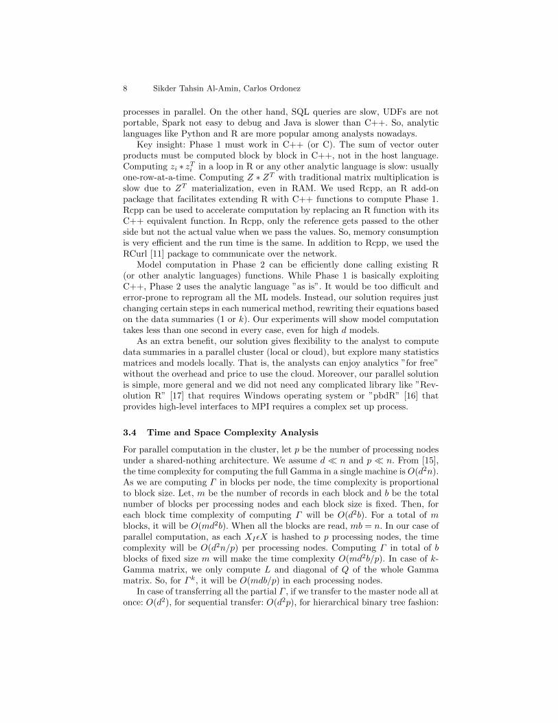
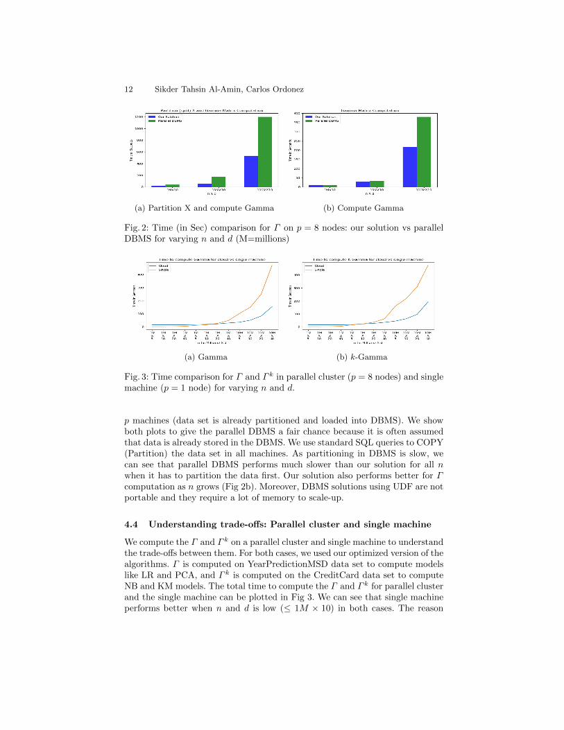
(a) Gamma (b) k-Gamma

Fig. 3: Time comparison for Γ and Γ k in parallel cluster (p = 8 nodes) and singlemachine (p = 1 node) for varying n and d.

p machines (data set is already partitioned and loaded into DBMS). We showboth plots to give the parallel DBMS a fair chance because it is often assumedthat data is already stored in the DBMS. We use standard SQL queries to COPY(Partition) the data set in all machines. As partitioning in DBMS is slow, wecan see that parallel DBMS performs much slower than our solution for all nwhen it has to partition the data first. Our solution also performs better for Γcomputation as n grows (Fig 2b). Moreover, DBMS solutions using UDF are notportable and they require a lot of memory to scale-up.

4.4 Understanding trade-offs: Parallel cluster and single machine

We compute the Γ and Γ k on a parallel cluster and single machine to understandthe trade-offs between them. For both cases, we used our optimized version of thealgorithms. Γ is computed on YearPredictionMSD data set to compute modelslike LR and PCA, and Γ k is computed on the CreditCard data set to computeNB and KM models. The total time to compute the Γ and Γ k for parallel clusterand the single machine can be plotted in Fig 3. We can see that single machineperforms better when n and d is low (≤ 1M × 10) in both cases. The reason


is, the parallel cluster is spending much time in partitioning the data set andtransferring the partial ΓI (or Γ k

I ) matrices. Parallel cluster seems to be morefaster from n = 1M and d = 20. When n is very high (n = 10M or more), theparallel cluster is at least 2X to 4X faster than the local machine. The reasonis, a single machine cannot scale as data size grows due to limited memory.However, the model computation part utilizing Γ or Γ k is almost same for both.So, the parallel cluster is the obvious choice when it comes to summarizing verylarge data sets.

5 Related Works

Summarization of scalable machine learning algorithms was done in a parallelmanner in [15]. However, this work was developed for a parallel array DBMS anddid not work for classification or clustering models. In this paper, we removedthe use of DBMS completely which was the main focus on [15]. We adaptedthe algorithm, generalized, and implemented such a way that it can work in aparallel cluster efficiently. Moreover, we introduced k-Gamma matrics that cancompute models like NB and KM which are significantly different from [15]. Wealso made use of reading data in blocks to read an infinite amount of inputdata. Similar to our proposed k-Gamma matrix, the summaries of [22] and [4]represent a (constrained) diagonal version of Γ because dimension independenceis assumed (i.e. cross-products, covariances, correlations are ignored) and thereis a separate vector to capture L. From a computational perspective, our Γcomputation boils down to one matrix multiplication, whereas those algorithmswork is aggregations. Also, our summarization is more general and it helps tocompute more complex models like LR, PCA, NB, and KM that could not besolved with older summaries. Parallel processing for data summarization hasreceived moderate attention. [12] highlights the following techniques: sampling,incremental aggregation, matrix factorization, and similarity joins. Research hasdeveloped fast algorithms based mostly on sampling, data summarization, andgradient descent [8], generally working in a sequential manner (data mining).Stochastic (incremental) gradient descent (SGD) [9] is a popular approach, usefulwhen there is a convex function to optimize (like least-squares in LR). As fordrawbacks, SGD is naturally sequential (difficult to process in parallel), it obtainsan approximate solution and it is difficult to adapt to non-convex functions (e.g.clustering).

From a “systems” angle, R combined with C++ did not exist and nobodythought we could insert efficient C++ code for a very common computation onparallel machines. However, R has been used for parallel computing on computerclusters, on multi-core systems, and in grid computing. There are many availablepackages in R for parallel computing and they are reviewed and compared in [18]based on development, usability, acceptance, and performance. There is a largebody of work on computing machine learning models in Hadoop “Big Data”systems, before with MapReduce [3] and currently with Spark [21]. On the otherhand, computing models with parallel DBMSs have received less attention [9],


[19] because they are considered cumbersome and more difficult to program. Thisarticle is a significant step forward and is fundamentally different from [5] whichworked only on a single machine. We introduced a new generalized algorithmto compute Γ in a parallel cluster. Also, we improved the k-Gamma algorithmwhere k summarization matrices (each d× d) were needed in [5] to compute NBand KM models. The improved algorithm needs only one matrix (d + 1 × 2k).Also, [5] cannot scale to big data as it was done in a local machine. Experimentalresults prove that our new solution does not have any limitation: neither mainmemory nor CPU power available.

6 Conclusions

We presented an improved 3-phase algorithm to compute ML models. Specifi-cally, we added a pre-processing phase, to partition and distribute the data set.Also, parallel processing is fully automated and we now cover a wide spectrumof unsupervised and supervised ML models. We introduced a general, parallel,summarization algorithm that can work across multiple programming languagesand platforms. We then studied how to integrate our parallel algorithm intothe R language, a popular language in ML and statistics. We justified why C++code is required and so we focused on optimizing summarization, with specializedC++ functions for a fundamental vector outer product, returning one or multipleGamma matrices (Γ k). We showed the actual model computation, fortunately,can be done with existing R functions, eliminating the need to reprogram them.An experimental evaluation shows our solution is either faster or more scalablethan Spark. On the other hand, our solution is remarkably faster than a previousprototype programmed with SQL queries and UDFs, the best previous solutionbased on the same approach.

Our research opens many possibilities for future work. We will tackle otherML models, including HMMs, LDA, and SVMs. We plan to compare tradeoffswhen integrating our algorithm with Python, another popular language withsignificantly different syntax and evaluation compared to R. Even though pro-cessing in one machine is slower than a parallel cluster, we intend to study howto accelerate computation with multicore CPUs and GPUs in a single box. Wewould like to encode our result summarization matrix in a general format thatcan be consumed by any langua ge or system. It should be feasible to detectintermediate computations in analytic source code, where our summarizationmatrix or matrices may accelerate or simplify processing.

References

1. Al-Jarrah, O.Y., Yoo, P.D., Muhaidat, S., Karagiannidis, G.K., Taha, K.: Efficientmachine learning for big data: A review. Big Data Research 2(3), 87–93 (2015)

2. Arthur, D., Vassilvitskii, S.: k-means++: the advantages of careful seeding. In:Proceedings of the Eighteenth Annual ACM-SIAM Symposium on Discrete Algo-rithms, SODA. pp. 1027–1035 (2007)


3. Behm, A., Borkar, V., Carey, M., Grover, R., Li, C., Onose, N., Vernica, R.,Deutsch, A., Papakonstantinou, Y., Tsotras, V.: ASTERIX: towards a scalable,semistructured data platform for evolving-world models. Distributed and ParallelDatabases (DAPD) 29(3), 185–216 (2011)

4. Bradley, P., Fayyad, U., Reina, C.: Scaling clustering algorithms to large databases.In: Proc. ACM KDD Conference. pp. 9–15 (1998)

5. Chebolu, S.U.S., Ordonez, C., Al-Amin, S.T.: Scalable machine learning in the Rlanguage using a summarization matrix. In: Database and Expert Systems Appli-cations - 30th International Conference, DEXA 2019, Linz, Austria, August 26-29,2019, Proceedings, Part II. pp. 247–262 (2019)

6. Dean, J., Corrado, G., Monga, R., Chen, K., Devin, M., Le, Q.V., Mao, M.Z., Ran-zato, M., Senior, A.W., Tucker, P.A., Yang, K., Ng, A.Y.: Large scale distributeddeep networks. In: Proc. Advances in Neural Information Processing Systems. pp.1232–1240 (2012)

7. Eddelbuettel, D.: Seamless R and C++ Integration with Rcpp. Springer, New York(2013)

8. Gemulla, R., Nijkamp, E., Haas, P., Sismanis, Y.: Large-scale matrix factorizationwith distributed stochastic gradient descent. In: Proc. KDD. pp. 69–77 (2011)

9. Hellerstein, J., Re, C., Schoppmann, F., Wang, D., Fratkin, E., Gorajek, A., Ng,K., Welton, C.: The MADlib analytics library or MAD skills, the SQL. Proc. ofVLDB 5(12), 1700–1711 (2012)

10. Hu, H., Wen, Y., Chua, T., Li, X.: Toward scalable systems for big data analytics:A technology tutorial. IEEE Access 2, 652–687 (2014)

11. Lang, D.T., Lang, M.D.T.: Package ‘rcurl’ (2012)12. Li, F., Nath, S.: Scalable data summarization on big data. Distributed and Parallel

Databases 32(3), 313–314 (2014)13. Ordonez, C., Cabrera, W., Gurram, A.: Comparing columnar, row and array dbmss

to process recursive queries on graphs. Information Systems (2016)14. Ordonez, C., Omiecinski, E.: Accelerating EM clustering to find high-quality solu-

tions. Knowledge and Information Systems (KAIS) 7(2), 135–157 (2005)15. Ordonez, C., Zhang, Y., Cabrera, W.: The Gamma matrix to summarize dense

and sparse data sets for big data analytics. IEEE Transactions on Knowledge andData Engineering (TKDE) 28(7), 1906–1918 (2016)

16. Ostrouchov, G., Chen, W.C., Schmidt, D., Patel, P.: Programming with big datain r (2012), http://r-pbd.org/

17. Rickert, J.: Big data analysis with revolution r enterprise. Revolution Analytics(2011)

18. Schmidberger, M., Morgan, M., Eddelbuettel, D., Yu, H., Tierney, L., Mansmann,U.: State-of-the-art in parallel computing with r. Journal of Statistical Software47 (2009)

19. Stonebraker, M., Abadi, D., DeWitt, D., Madden, S., Paulson, E., Pavlo, A., Rasin,A.: MapReduce and parallel DBMSs: friends or foes? Commun. ACM 53(1), 64–71(2010)

20. Xing, E.P., Ho, Q., Dai, W., Kim, J.K., Wei, J., Lee, S., Zheng, X., Xie, P., Kumar,A., Yu, Y.: Petuum: A new platform for distributed machine learning on big data.IEEE Trans. Big Data 1(2), 49–67 (2015)

21. Zaharia, M., Chowdhury, M., Franklin, M., Shenker, S., Stoica, I.: Spark: Clustercomputing with working sets. In: HotCloud USENIX Workshop (2010)

22. Zhang, T., Ramakrishnan, R., Livny, M.: BIRCH: An efficient data clusteringmethod for very large databases. In: Proc. ACM SIGMOD Conference. pp. 103–114(1996)

Documents

Scalable Machine Learning on Popular Analytic Languages